Due Date:2/1/2014 Date submitted: Programme Title: Course No.: Tutor: Assessment Cover Sheet Complete and attach this cover sheet to your assessment before submitting Course Title: Student ID: 201000754 Student Name: Mustafa Isa Al-Ansari Mustafa Isa Al-Ansari 201000754 Assessment Title Mr. John leek By submitting this assessment for marking, either electronically or as hard copy, I confirm the following: This assignment is our own work Any information used has been properly referenced. I understand that a copy of my work may be used for moderation. I have kept a copy of this assignment Instrumentation and control ENB5230 Bachelor of Engineering Technology Water jig
Transcript
Due Date:2/1/2014 Date submitted:
Programme Title:
Course No.:
Tutor:
Assessment Cover SheetComplete and attach this cover sheet to your assessment before submitting
Course Title:
Student ID: 201000754
Student Name: Mustafa Isa Al-Ansari
Mustafa Isa Al-Ansari 201000754
Assessment Title
Mr. John leek
By submitting this assessment for marking, either electronically or as hard copy, I confirm the following:
This assignment is our own work Any information used has been properly referenced. I understand that a copy of my work may be used for moderation. I have kept a copy of this assignment
Instrumentation and control
Bachelor of Engineering Technology
ENB5230
Water jig
Mustafa Isa Al-Ansari 201000754
Abstract
The main aim of this project is to design a program that can measure the water jig level using Lab VIEW. For example, if the water level is six cm the program should measure the level by pressure sensor and copy it on the screen. the system was done by connecting the pump and the pressure sensor to LabVIEW to control the pump, and getting feedback from the pressure sensor. after that A PID control was added to the program to troubleshoot the errors in the system. This was followed by tuning the system to find the best value of the gains such as Kc, Ti and Td and explain why they are the best values. finally a simulation model was added to modify the system to make it response better. this report will go in details on how the system was operated, tuned and simulated.
Objective
Using LabVIEW configure the Water pump level jig with a 3 term PID controller Operate the pressure sensor and the pump Tuning the system to get the best values of PID Create a system modelling to modify the real system Labview (first order model with Padé
delay) with a 3-term PID controller Compare the simulation results with the real system results
Mustafa Isa Al-Ansari 201000754
Table of ContentsAbstract.......................................................................................................................................................2
Proportional control only......................................................................................................................23
Proportional and integral control only..................................................................................................28
Proportional, Integral and Derivative control........................................................................................32
System modeling.......................................................................................................................................33
Figure 1 PWM circuit...................................................................................................................................8Figure 2 Deterring C2 for adjust the frequency of the PWM circuit..........................................................10Figure 3MOSFET drive board.....................................................................................................................12Figure 4 Pump oberarion...........................................................................................................................17Figure 5 calibration result..........................................................................................................................19Figure 6 open loop system........................................................................................................................20Figure 7 close loop system.........................................................................................................................21Figure 8the final version of the program ( includes PID controller)...........................................................22Figure 9 simulation model.........................................................................................................................33Figure 10 calculating Ks.............................................................................................................................34Figure 11 the result of the simulation model............................................................................................35
Table 1 how good does the pump work....................................................................................................11Table 2 the gain and offset values.............................................................................................................18Table 3 testing the system.........................................................................................................................18Table 4 caliration results............................................................................................................................19Table 5 best value of td.............................................................................................................................32
Mustafa Isa Al-Ansari 201000754
Introduction:
Explanation of my project:In this project, I have been given a tank consists of pressure sensor, and water pump. I was asked to connect these two components in LabVIEW to control the level of the water in the tank. here are the main step that were followed to accomplish the objectives of the project.
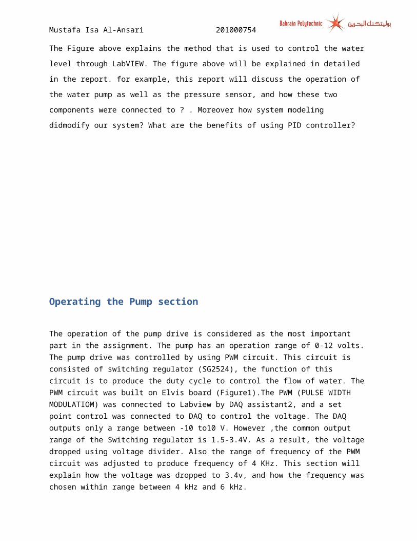
The Figure above explains the method that is used to control the water level through LabVIEW. The
figure above will be explained in detailed in the report. for example, this report will discuss the
operation of the water pump as well as the pressure sensor, and how these two components were
connected to ? . Moreover how system modeling didmodify our system? What are the benefits of using
PID controller?
Ao0 A circuit was built on Elvis board (PWM)
MOSFET driver
pum
filling the tank
pressure sensor works
Instrumentation
Low pass filter
AI0 PID GRAPH
AI0 10 v
Mustafa Isa Al-Ansari 201000754
Operating the Pump section
The operation of the pump drive is considered as the most important part in the assignment. The pump has an operation range of 0-12 volts. The pump drive was controlled by using PWM circuit. This circuit is consisted of switching regulator (SG2524), the function of this circuit is to produce the duty cycle to control the flow of water. The PWM circuit was built on Elvis board (Figure1).The PWM (PULSE WIDTH MODULATIOM) was connected to Labview by DAQ assistant2, and a set point control was connected to DAQ to control the voltage. The DAQ outputs only a range between -10 to10 V. However ,the common output range of the Switching regulator is 1.5-3.4V. As a result, the voltage dropped using voltage divider. Also the range of frequency of the PWM circuit was adjusted to produce frequency of 4 KHz. This section will explain how the voltage was dropped to 3.4v, and how the frequency was chosen within range between 4 kHz and 6 kHz.
Constructing PWM circuit
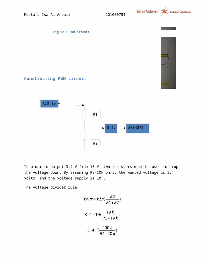
Figure 1 PWM circuit
Mustafa Isa Al-Ansari 201000754
In order to output 3.4 V from 10 V. two resistors must be used to drop the voltage down. By assuming R2=10k ohms, the wanted voltage is 3.4 volts, and the voltage supply is 10 V
The voltage divider rule:
Vout=Vin( R2R1+R2
)
3.4=10( 10kR1+10k
)
3.4=( 200 kR1+20k
)
3.4 R1+68k=20k
3.4 R1=(100 k−34 k )
3.4 R1=66K
R1=20K
Mustafa Isa Al-Ansari 201000754
The value of the frequency of the PWM circuit was chosen from the figure below . So first of all
The Value of the C2 that was determined is equal to 0.1 uF , also it was important to determine the value of R4, so the equation below was done:
BY assuming the wanted frequency which is 4 KHz
f=( 1.30R4∗c2
)
4 Khz=( 1.30R 4∗0.1uf
)
R4=3.250Kohms
The closest value of R4 was used because there is no such a resistor in the store that has a value of 3.250Kohms, so a 3.3 K ohms. If this value is substituted in the equation the value of the frequency will be 3.9 KHz, but it is acceptable to have that value of frequency.
Figure 2 Deterring C2 for adjust the frequency of the PWM circuit.
Mustafa Isa Al-Ansari 201000754
Testing PWM Circuit
After a dropping the Voltage from 10 Volts- 3.4 volts, and adjusting the frequency of the circuit, test was done to the circuit to check how good the circuit is.
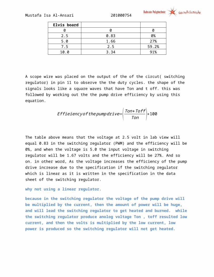
Table 1 how good does the pump work
Output Volts from Elvis board
Input volts to switching (analogue) Pump drive %
0 0 02.5 0.83 0%5.0 1.66 27%7.5 2.5 59.2%
10.0 3.34 91%
A scope wire was placed on the output of the of the circut( switching regulator) in pin 11 to observe the the duty cycles. the shape of the signals looks like a square waves that have Ton and t off. this was followed by working out the the pump drive efficiency by using this equation.
Effieiency of the pumpdrive=(Ton+ToffTon )∗100
The table above means that the voltage at 2.5 volt in lab view will equal 0.83 in the switching regulator (PWM) and the efficiency will be 0%, and when the voltage is 5.0 the input voltage in switching regulator will be 1.67 volts and the efficiency will be 27%. And so on. in other word, As the voltage increases the efficiency of the pump drive increase due to the specification if the switching regulator which is linear as it is written in the specification in the data sheet of the switching regulator.
why not using a linear regulator.
because in the switching regulator the voltage of the pump drive will be multiplied by the current, then the amount of power will be huge, and will lead the switching regulator to get heated and burned. while the switching regulator produce anolog voltage Ton , toff resulted low current, and then the volts is multiplied by the low current, low power is produced so the switching regulator will not get heated.
Mustafa Isa Al-Ansari 201000754
MOSFET
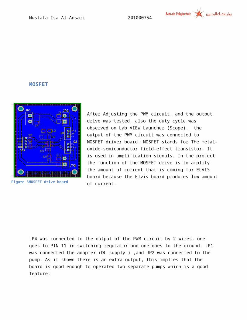
After Adjusting the PWM circuit, and the output drive was tested, also the duty cycle was observed on Lab VIEW Launcher (Scope). the output of the PWM circuit was connected to MOSFET driver board. MOSFET stands for The metal–oxide–semiconductor field-effect transistor. It is used in amplification signals. In the project the function of the MOSFET drive is to amplify the amount of current that is coming for ELVIS board because the Elvis board produces low amount of current.
JP4 was connected to the output of the PWM circuit by 2 wires, one goes to PIN 11 in switching regulator and one goes to the ground. JP1 was connected the adapter (DC supply ) ,and JP2 was connected to the pump. As it shown there is an extra output, this implies that the board is good enough to operated two separate pumps which is a good feature.
Figure 3MOSFET drive board
Mustafa Isa Al-Ansari 201000754
.
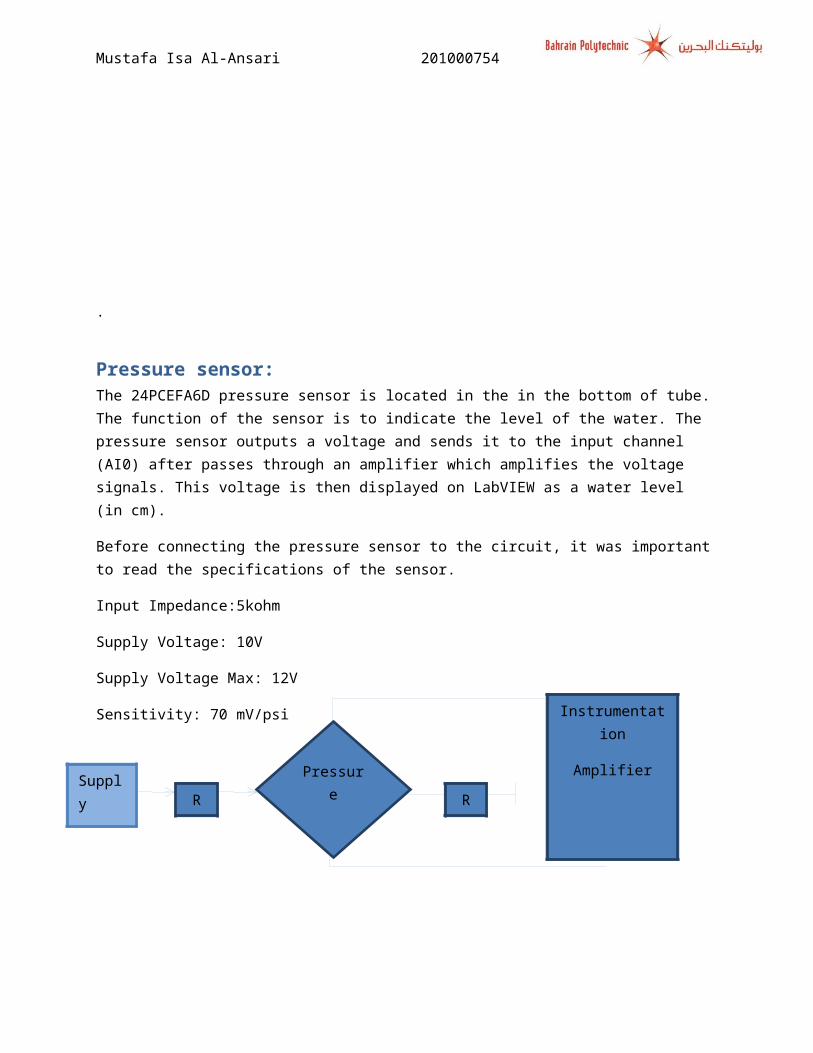
Pressure sensor:The 24PCEFA6D pressure sensor is located in the in the bottom of tube. The function of the sensor is to indicate the level of the water. The pressure sensor outputs a voltage and sends it to the input channel (AI0) after passes through an amplifier which amplifies the voltage signals. This voltage is then displayed on LabVIEW as a water level (in cm).
Before connecting the pressure sensor to the circuit, it was important to read the specifications of the sensor.
Input Impedance:5kohm
Supply Voltage: 10V
Supply Voltage Max: 12V
Sensitivity: 70 mV/psi
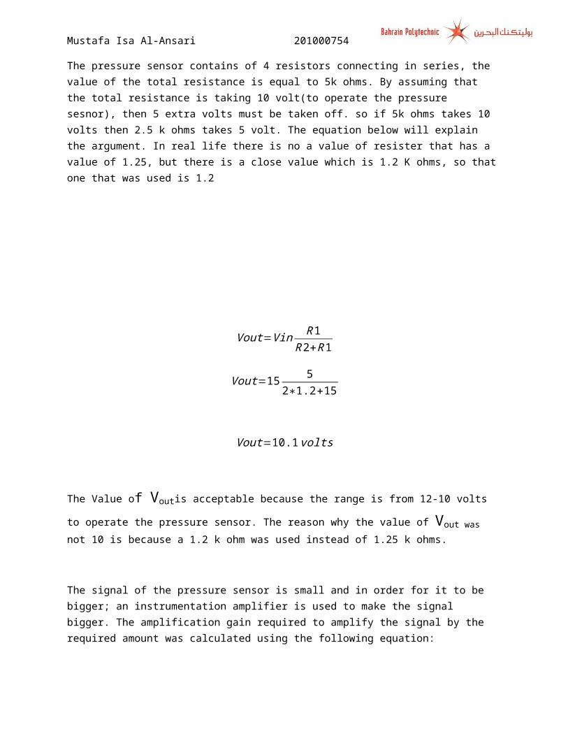
The pressure sensor contains of 4 resistors connecting in series, the value of the total resistance is equal to 5k ohms. By assuming that the total resistance is taking 10 volt(to operate the pressure sesnor), then 5 extra volts must be taken off. so if 5k ohms takes 10 volts then 2.5 k ohms takes 5 volt. The equation below will explain the argument. In real life there is no a value of resister that has a value of 1.25, but there is a close value which is 1.2 K ohms, so that one that was used is 1.2
Supply
(15v)R R
Pressure
Sensor
Instrumentation
Amplifier
Mustafa Isa Al-Ansari 201000754
Vout=Vin R1R2+R1
Vout=15 52∗1.2+15
Vout=10.1 volts
The Value of Voutis acceptable because the range is from 12-10 volts to operate the pressure sensor.
The reason why the value of Vout was not 10 is because a 1.2 k ohm was used instead of 1.25 k ohms.
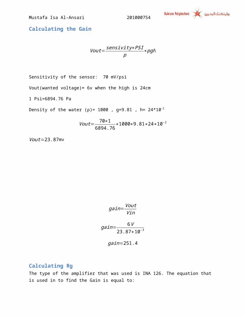
The signal of the pressure sensor is small and in order for it to be bigger; an instrumentation amplifier is used to make the signal bigger. The amplification gain required to amplify the signal by the required amount was calculated using the following equation:
Calculating the Gain
Vout= sensivity∗PSIp
∗pgh
Sensitivity of the sensor: 70 mV/psi
Vout(wanted voltage)= 6v when the high is 24cm
1 Psi=6894.76 Pa
Density of the water (ρ)= 1000 , g=9.81 , h= 24*10-2
Vout= 70∗16894.76
∗1000∗9.81∗24∗10−2
Vout=23.87mv
Mustafa Isa Al-Ansari 201000754
gain=VoutVin
gain= 6V23.87∗10−3
gain=251.4
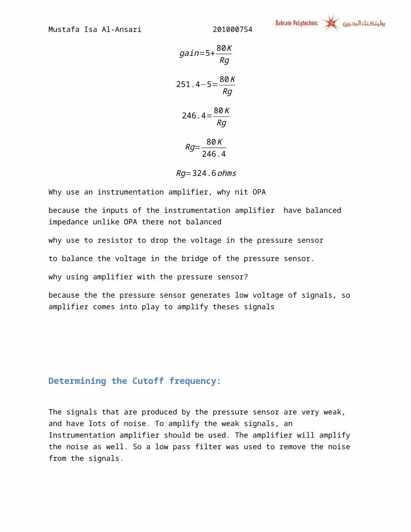
Calculating RgThe type of the amplifier that was used is INA 126. The equation that is used in to find the Gain is equal to:
gain=5+ 80KRg
251.4−5=80KRg
246.4=80KRg
Rg= 80K246.4
Rg=324.6 ohms
Why use an instrumentation amplifier, why nit OPA
because the inputs of the instrumentation amplifier have balanced impedance unlike OPA there not balanced
why use to resistor to drop the voltage in the pressure sensor
to balance the voltage in the bridge of the pressure sensor.
why using amplifier with the pressure sensor?
because the the pressure sensor generates low voltage of signals, so amplifier comes into play to amplify theses signals
Mustafa Isa Al-Ansari 201000754
Determining the Cutoff frequency:
The signals that are produced by the pressure sensor are very weak, and have lots of noise. To amplify the weak signals, an Instrumentation amplifier should be used. The amplifier will amplify the noise as well. So a low pass filter was used to remove the noise from the signals.
A low pass filter consists of a resistor connected to a capacitor (that’s connected to the ground) in series. LPF designed to reject unwanted frequencies of an electric signal. The filter should pass frequencies that are less than 10 Hz, so the cutoff frequency is 10 0Hz.
fc=( 12∗pi∗R∗C
)
10=( 12∗pi∗22k∗C
)
C=( 12∗pi∗22K∗10
)
C=0.72uf ¿
It was hard to find the exact value of capacitor, so a close value to it was used which is 0.45uf+0.45uf
Mustafa Isa Al-Ansari 201000754
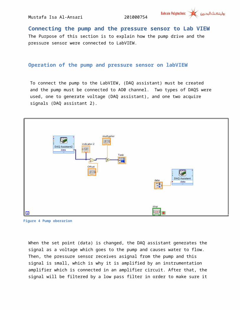
Connecting the pump and the pressure sensor to Lab VIEWThe Purpose of this section is to explain how the pump drive and the pressure sensor were connected to LabVIEW.
Operation of the pump and pressure sensor on labVIEW
To connect the pump to the LabVIEW, (DAQ assistant) must be created and the pump must be connected to AO0 channel. Two types of DAQS were used, one to generate voltage (DAQ assistant), and one two acquire signals (DAQ assistant 2).
When the set point (data) is changed, the DAQ assistant generates the signal as a voltage which goes to the pump and causes water to flow. Then, the pressure sensor receives asignal from the pump and this signal is small, which is why it is amplified by an instrumentation amplifier which is connected in an amplifier circuit. After that, the signal will be filtered by a low pass filter in order to make sure it does not have any noise in it. The filtered signal is then sent to the Labview program as a voltage signal acquired through the DAQ assistant2. When the level of the water is zero in the real system, it does not match the level in labview. It goes to a value that is less than zero, AS a result an Indicator was placed to observe the value when the level is zero, and then a subtractor was added to take off this value. The output voltage of DAQ assistant 2 has a minimum voltage of -10V and a maximum voltage of 10V,
Figure 4 Pump oberarion
Mustafa Isa Al-Ansari 201000754
therefore a multiplier was used in order to multiply the voltage and make it reach 24V which is the voltage needed to make the water go to its maximum 24 cm value.
Table 2 the gain and offset values
Calibration gain required Zero offset required3.59 -2.2
Water level calibration results (open loop)
After adjusting the Block diagram, and testing the system, we have noticed that when we run the system at different levels, the displayed water level in front panel matches the levels in the real water jig. However, there was very small difference in the two values (Lab VIEW tank and water jig tube). The table below is done to show the error between them.
The following table illustrates the open loop water level calibration results
Table 3 testing the system
Water level reading (cm water) Displayed water level on LabView front panel
% error in values
0 0 05 5 0%
10 10 0%15 15 0%20 19.9 0.5%24 23.6 1.6%
Calibration
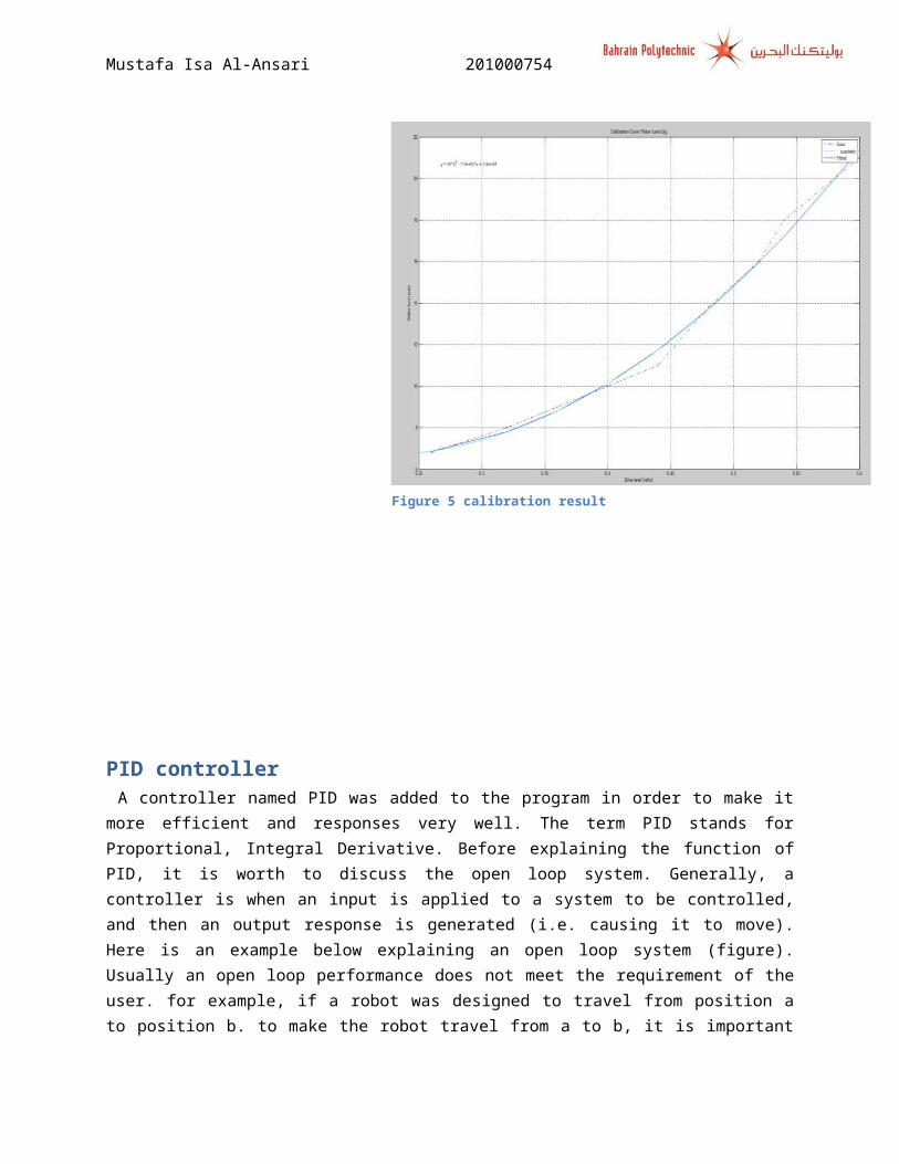
After adjusting the pump drive ,the pressure sensor, and making sure the pressure sensor measues the the level of the water accurately, a graph on Matlab was plotted to see the response of the system. the graph represents the height(the level of the water Against the Pump drive (voltage). First of all the a table was made to record the the values of the pump drive and the level of the water.
Mustafa Isa Al-Ansari 201000754
Table 4 caliration results
Input Voltage pump drive (Volts) Water Level (cm)6.25 volt 5 cm
6.3 7cm6.35 8.3 cm6.4 10 cm
6.45 12.2 cm6.5 15 cm
6.55 18 cm 6.6 22 cm
The response of the figure is clear; the system has a quadratic response. This means that the gain of the system is different depends on the level of the water. For example, the values of the gain at 10 cm are different at 18 cm that is because the slop is changing at these levels.
Figure 5 calibration result
Mustafa Isa Al-Ansari 201000754
PID controller A controller named PID was added to the program in order to make it more efficient and responses very well. The term PID stands for Proportional, Integral Derivative. Before explaining the function of PID, it is worth to discuss the open loop system. Generally, a controller is when an input is applied to a system to be controlled, and then an output response is generated (i.e. causing it to move). Here is an example below explaining an open loop system (figure). Usually an open loop performance does not meet the requirement of the user. for example, if a robot was designed to travel from position a to position b. to make the robot travel from a to b, it is important to measure the speed of the robot, and how long it takes to reach point b, then it will be simple to the robot to stop at position b. However, if the position A is changed or the speed of the robot has slightly changed, then the robot will not stop at point b. because it cannot make an adjustment by it is own. Now, the solution is feedback control which means sensing the output of the plant and feeding it back, so then the system could make adjustment accordingly. However, there is an error occurred between the desired value and the measured value. For example, the error is the delta between where the object is and where it wants to go. So in case of the robot the error will be the difference between the references position which is the distance between a-b, and the robot current position. So there must be a method that causes the robot to eventually reach the desired position accurately, and this is exactly what a controller does. It takes the errors signals and converts it into a command and sends it to the plant. One of the goals of control engineers is to design this controller that the difference between the reference signals to the desire signal is driven to zero. There are many types of controllers, one of the most popular one is called PID controller. PID controller stands for proportional, integral, derivative. Each of these parameters has a responsibility of treating the error. The table below explains the function of eat parameter ( KP,Ki,Kd).
Figure 6 open loop system
Figure 7 close loop system
Parameters Rise time/Time Constant Overshoot Settling time Steady state
error (SSE)Stability
(Oscillation)Kp Decrease Increase Very less effect Decrease Degrades
Mustafa Isa Al-Ansari 201000754
Ki Decrease Increase Increase Eliminates DegradesKd Very less effect Decrease Decrease No effects Degrades
PID measurement resultsThis section will include the reason behind choosing the specific value of Kc, Ti, and Td.
Mustafa Isa Al-Ansari 201000754
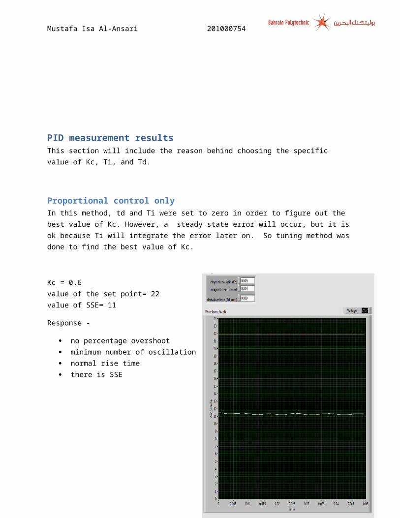
Proportional control only In this method, td and Ti were set to zero in order to figure out the best value of Kc. However, a steady state error will occur, but it is ok because Ti will integrate the error later on. So tuning method was done to find the best value of Kc.
Kc = 0.6 value of the set point= 22 value of SSE= 11
Response -
no percentage overshoot minimum number of oscillation normal rise time there is SSE
Kc = 1 value of the set point= 22 value of SSE= 16
Response -
the system is not stable
Mustafa Isa Al-Ansari 201000754
there is oscillations very fast rise time there is SSE
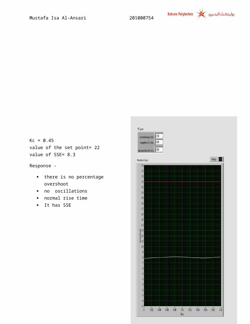
Kc = 0.45 value of the set point= 22 value of SSE= 8.3
Response -
Mustafa Isa Al-Ansari 201000754
there is no percentage overshoot no oscillations normal rise time It has SSE
The Best value of Kc is 0.6 because:
there is no overshoot very low number of oscillations the rise time was normal Maximum steady state error
Mustafa Isa Al-Ansari 201000754
The value of steady state error changes when the level of the set point is changed. That is because the system has a quadratic equation (nonlinear) which means the slop is changing at different levels. Therefore, the user should change the gain at different levels
Mustafa Isa Al-Ansari 201000754
Mustafa Isa Al-Ansari 201000754
Proportional and integral control only
In this section, tuning method was used to find the best value of Ti. Also the best value of Kc was used in this section, and it was fixed.
Ti=0.01 min value of the set point= 22 over shoot value = it was over 24 cm
Response -
there is percentage overshoot many numbers of oscillations fast rise time
Mustafa Isa Al-Ansari 201000754
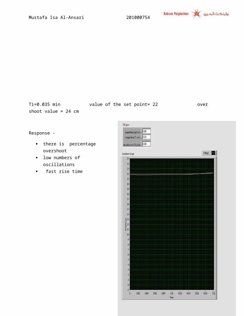
Ti=0.035 min value of the set point= 22 over shoot value = 24 cm
Response -
there is percentage overshoot low numbers of oscillations fast rise time
Mustafa Isa Al-Ansari 201000754
Ti=0.045 min value of the set point= 22 over shoot value = no overshoot
Response -
no percentage overshoot no oscillations normal rise time No SEE
Mustafa Isa Al-Ansari 201000754
The Best value of Kc is 0.6, and Ti is 0.045 because:
there is no overshoot very low number of oscillations the rise time was normal no steady state error the system was stable
In this method, the value of Kc was fixed because it was found as the best value in proportional gain section. The Ti was changed till the best value is found which is the best value because there was not overshoot, low number of oscillations, the rise time is normal, the steady state error does not exist, and the system was stable. However, the value of Kc, and Ti are only good at 22 cm. If the set point is changed, then the system will not stay stable anymore because the system is nonlinear .The only way to fix this problem is gain scheduler. Firstly, the user should tune and record the best value of Kc, and Ti, and then put the best values in gain scheduler. Finally, the system wills response very well according to the level of the water.
Mustafa Isa Al-Ansari 201000754
Proportional, Integral and Derivative control
Table 5 best value of td
K p Ti and T d Overshoot value Response0.6 0.045 0.01 Over 24 cm Not stable0.6 0.045 0.001 Over 24 cm Not stable0.6 0.045 0 No over shoot stable
When Td is added to the system, it goes unstable because the Td differentiate the noise, resulted the system to become unstable. To fix this problem, the value Td should be set to zero.
Mustafa Isa Al-Ansari 201000754
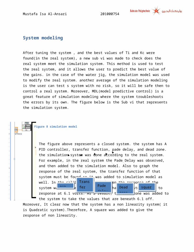
System modeling
After tuning the system , and the best values of Ti and Kc were found(in the real system), a new sub vi was made to check does the real system meet the simulation system. This method is used to test the real system, and it allows the user to predict the best value of the gains. in the case of the water jig, the simulation model was used to modify the real system. another average of the simulation modeling is the user can test s system with no risk, so it will be safe then to control a real system. Moreover, MDL(model predictive control) is a great feature of simulation modeling where the system troubleshoots the errors by its own. The figure below is the Sub vi that represents the simulation system.
The figure above represents a closed system. the system has A PID controller, transfer function, pade delay, and dead zone. the simulation system was done according to the real system. For example, in the real system the Pade Delay was observed, and then added to the simulation model. Also to graph the response of the real system, the transfer function of that system must be found so it was added to simulation model as well. In the calibration section when the response of the system was observed, it was clear that the system starts to response at 6.1 volts. As a result, the dead zone was added to the system to take the values that are beneath 6.1 off. Moreover, It clear now that the system has a non linearity system( it is Quadratic system).Therefore, A square was added to give the response of non linearity.
PID controllerthe type of the PID controller is Academic. it is different than parallel PID. In the parallel PID each gains act by its own. In other word, Kp ,Ki, an Kd do not depend on each other. Where
in the Acadimic PID, it is different each gain depend on the other ( Ki, and Kd depends onKp). The value of Ti in the real system is given in second where in the simulation model it is given in min so it was multiplied by 60.
Figure 8 simulation model
PIDTransfer Pade
delayDead zone
square
Mustafa Isa Al-Ansari 201000754
Transfer function The value of the gain Ks was calculated by setting Ti and Td to zero, and adjusted Kc till the system is
stabled. the equation below was used to find the value if Ks.
¿out
=1+( 1ks∗kp
)
228
=1+( 1ks∗0.6
)
ks=1.2
Then the value of the time constant was adjusted till the system response very well. and that is exactly what happened to the pade delay, it was changes till the system responses very well. By changing the bade dealy the phase was changing so it was giving a better results when the delay is changed.
Figure 9 calculating Ks
Mustafa Isa Al-Ansari 201000754
Conclusion:In conclusion, the aim of this project was to design a labview program that could maintain the level of the water by using PID controller. There were two main devices which are Pump , and pressure sensor. both were operated, tested and connected to labview. After that, the system became closed because PID controller was added to the program. This was followed by tuning the system to find the best values
Figure 10 the result of the simulation model
Mustafa Isa Al-Ansari 201000754
of kc and ti, td. However, Td was not used because it makes the system worse and worse by differentiating the noise of the signals. finally the simulation modeling was added to the system to modify the parameter Kc and ti , and make the real system responses better by observing the response of the simulation result.
Explain how the program works :
Here is an explanation of the program: First of all, when the user changes the set point control that is connected to PID, an outpus is generated and passes though a division because the set point is from 0-24 so it divided it by 2.4 so the signal will be out 10 because the DAQ can only read signals from 0-10 volts, then it passes through DAQ assistant, so the signal will output from channel Ao0. After that, the signals goes to the pump after passes through PWM, leading the pump to operate, and filling the tube. Then the pressure sends signals to AI0 after passing though t amplifier and low pass filter. So it come in from DAQ assistant 2. After that the signal multiplied by 2.4 because the DAQ assistant 2 only outputs 0-10 volts so the signals will be presented out of 24 cm it the graph.