151


Abstract
Increased interest in the launch of nanosatellites has driven the development of
alternative, more efficient, rocket nozzles. One such option is the dual-bell nozzle (DBN), in
which the geometry is designed to achieve two ideal design points over the ascent profile,
resulting in a higher average specific impulse for the booster stage compared to a conventional
nozzle. This project involved the design of a DBN, which was then modeled using ANSYS
Fluent. A scaled DBN was also fabricated and tested in an indraft supersonic wind tunnel.
Results from the experimental characterization of the DBN, using schlieren imaging of flow
structures, are presented and found to be qualitatively consistent with simulation results. Results
of the Fluent simulations for a full-scale DBN and the scaled DBN tested in the wind tunnel are
also presented.
“Certain materials are included under the fair use exemption of the U.S. Copyright Law and have been prepared according to the fair use guidelines and are restricted from further use."
i

Acknowledgements
We would like to thank the following individuals and groups for their help and support throughout the entirety of this project:
Professor John Blandino for providing direction and guidance as our project
advisor
Zach Taillefer for running the vacuum chamber during wind tunnel testing
Kevin Arruda and Matt DiPinto for helping with the machining of the wind tunnel
Jonathon Jones for providing NanoLaunch vehicle data and ascent profiles
Professor Adrianna Hera for providing Fluent instruction
ii

Authorship
Section Author Introduction HLGM Background 2.1, 2.1.2, 2.1.3 KBD 2.1.1, 2.2 HLGM 2.3 ECF 2.4.1, 2.4.2 MWH 2.4.3, 2.4.4 HJP Methodology 3.1 KBD 3.2 ECF 3.3 HJP 3.4, 3.5 HLGM Experimental Procedures 4.1.1, 4.1.2, 4.1.3, 4.1.4, 4.2.3 KBD 4.3, 4.3.1 ECF 4.3.2, 4.3.3 KBD Numerical Simulation 5.1.1, 5.3.2 HLGM 5.1.2, 5.3.3, 5.3.4 HJP 5.2, 5.3.1 MWH Analysis and Discussion 6.1 HJP 6.2 HLGM 6.3 ECF Conclusion and Recommendations for Future Work 7.1 HLGM 7.2 MWH Appendix A: AIAA Paper ALL Appendix B: How to use the Schlieren System KBD Appendix C: Fluent Contours of Pressure HLGM, HJP, MWH Appendix D: Parabolic Coefficient Calculations HLGM Appendix E: Matlab Script HLGM
iii

Table of Contents
Abstract ................................................................................................................................ i
Acknowledgements ............................................................................................................. ii
Authorship.......................................................................................................................... iii
Table of Contents ............................................................................................................... iv
Table of Figures ............................................................................................................... viii
Table of Tables ................................................................................................................. xii
1 Introduction .................................................................................................................. 1
2 Background ................................................................................................................... 3
2.1 Nozzle Background ............................................................................................... 3
2.1.1 Advanced Nozzles ........................................................................................... 6
2.1.2 Dual-Bell Nozzle History ................................................................................ 9
2.1.3 Nozzle Comparisons ..................................................................................... 10
2.2 Application .......................................................................................................... 13
2.3 Schlieren Imaging ............................................................................................... 14
2.3.1 Optical Principles .......................................................................................... 15
2.3.2 Applications to Flow Regimes ...................................................................... 16
2.3.3 Schlieren vs. Shadowgraph Techniques ........................................................ 17
2.3.4 Schlieren System Types ................................................................................ 18
iv

2.4 Computational Fluid Dynamics .......................................................................... 19
2.4.1 Flow Regimes ................................................................................................ 19
2.4.2 Turbulence Models ........................................................................................ 20
2.4.3 FEM vs. FVM ............................................................................................... 21
2.4.4 Turbulence Model Comparisons ................................................................... 22
3 Methodology ............................................................................................................... 25
3.1 Supersonic Wind Tunnel ..................................................................................... 25
3.2 Schlieren System ................................................................................................. 26
3.3 COMSOL vs. Fluent ........................................................................................... 28
3.4 Thrust Optimized Parabolic Contours ................................................................. 29
3.5 Dual-Bell Nozzle Design .................................................................................... 33
4 Experimental Procedures ............................................................................................ 37
4.1 Setup and Experiments ........................................................................................ 37
4.1.1 Alignment and Focusing ............................................................................... 37
4.1.2 Updates to Existing Schlieren System .......................................................... 38
4.1.3 Optimization and Specific Setup ................................................................... 41
4.1.4 System Validation Experiments .................................................................... 44
4.2 Manufacturing Test Nozzles ............................................................................... 48
4.2.1 CAD Nozzle Modeling .................................................................................. 49
4.2.2 Manufacturing Constraints ............................................................................ 50
v


6.2 Full-Scale Nozzle Performance Comparison .................................................... 100
6.3 Physical Interpretation ....................................................................................... 102
7 Conclusion and Recommendations for Future Work ............................................... 104
7.1 Conclusion ......................................................................................................... 104
7.2 Recommendations for Future Work .................................................................. 105
8 References ................................................................................................................ 108
Appendix A: AIAA Paper ............................................................................................... 110
Appendix B: How to Use the Schlieren System ............................................................. 120
Appendix C: Fluent Contours of Pressure ...................................................................... 122
Appendix D: Parabolic Coefficient Calculations ............................................................ 127
Appendix E: MATLAB Scripts ...................................................................................... 130
vii

Table of Figures
Figure 1: A Dual-Bell Nozzle [Copyright ©Nasuti, F., Onofri, M., & Martelli, E., 2005
[4]]....................................................................................................................................... 5
Figure 2: Rao Parabolic Contour [Copyright Kulhanek 2012[6]] ...................................... 7
Figure 3: FSS vs. RSS within a conventional nozzle [Copyright © Hagemann and Frey
2008 [8]].............................................................................................................................. 8
Figure 4: A shadowgram (left) and a schlieren image (right) [Copyright © Settles 2001
[13]]................................................................................................................................... 17
Figure 5: Conventional Z-type system [Copyright © Settles 2001 [13]] ......................... 18
Figure 6: A body placed in incompressible and compressible flow [Copyright © Auld and
Srinivas 2006 [16]] ........................................................................................................... 19
Figure 7: Flow near boundary layer for laminar and turbulent flow [Copyright © NASA
Glenn Research center 2000 [17]] .................................................................................... 20
Figure 8: Existing Schlieren setup. ................................................................................... 26
Figure 9: TOP nozzle based on Rao's approximation [Copyright © Kulhanek, 2012 [6]].
........................................................................................................................................... 30
Figure 10: Rao Contours for different altitudes ................................................................ 33
Figure 11: Dual-bell contour connecting two Rao contours designed for different ambient
pressures ............................................................................................................................ 34
Figure 12: Dual-bell nozzle with normalized axes ........................................................... 35
Figure 13: Dual-bell nozzle with labeled sections (axes scaled for clarity) ..................... 35
Figure 14: Solid model of optical plate............................................................................. 40
Figure 15: Schlieren image of a candle flame .................................................................. 45
viii

Figure 16: Schlieren image of a heat gun ......................................................................... 46
Figure 17: Schlieren Image of a Jet of Air ........................................................................ 46
Figure 18: Schlieren image of the interference between a candle flame and a jet of air .. 47
Figure 19: Schlieren image of non-interference between a candle flame and a jet of air . 48
Figure 20: SSWT CAD model from the 2013 MQP [27] ................................................. 50
Figure 21: CAD model of new set-up with dual-bell contours ......................................... 50
Figure 22: Wind tunnel set-up .......................................................................................... 52
Figure 23: Test section with labeled parts ........................................................................ 53
Figure 24: Fixture plate attached to CNC machine .......................................................... 54
Figure 25: Dual-bell contour during machining process using the fixture plate .............. 55
Figure 26: Lap joint used for O-ring joining surfaces ...................................................... 57
Figure 27: Test Setup ........................................................................................................ 58
Figure 28: Normal shock with Rao Contours ................................................................... 60
Figure 29: Normal Shock with Angled Shape in Rao Contours ....................................... 61
Figure 30: Early Development of Boundary Layer Structures ......................................... 62
Figure 31: Advanced Development of Boundary Layer Structures .................................. 62
Figure 32: Shock structure at inflection point ................................................................... 63
Figure 33: Boundary layer flow features .......................................................................... 64
Figure 34: Throat region shock and boundary feature ...................................................... 65
Figure 35: Series of boundary flow features ..................................................................... 65
Figure 36: Rao nozzle mesh with downstream section ..................................................... 66
Figure 37: Dual bell nozzle mesh with downstream section ............................................ 68
Figure 38: Rao Wind Tunnel Contour Mesh .................................................................... 70
ix

Figure 39: Dual-Bell Wind Tunnel Contour Mesh ........................................................... 70
Figure 40: Key for Table 8 ................................................................................................ 73
Figure 41: Fluent method of solving governing equations [Copyright © Fluent Inc., 2006]
........................................................................................................................................... 75
Figure 42: Rao Mach contours with chamber pressures of 101325 Pa (1 atm) and back
pressures of a) 6.6 Pa, b) 100 Pa, c) 10,000 Pa ................................................................. 78
Figure 43: Rao Mach contours with chamber pressures of 101325 Pa and back pressures
of a) 25,000 Pa and b) 50,000 Pa ...................................................................................... 79
Figure 44: Rao Mach contour with a chamber pressure of 1 atm and a back pressure of
75,000 Pa........................................................................................................................... 80
Figure 45: Dual-bell Mach contours. Top design pressure to 35.7 Pa; bottom atmospheric
pressure to 35.7 Pa ............................................................................................................ 82
Figure 46: Dual-bell Mach contours for design point pressure ratios of 150 (top) and 1000
(bottom)............................................................................................................................. 84
Figure 47: Dual-bell Mach contours for pressure ratios of 4.05, 10, and 20.26 in order
from top to bottom ............................................................................................................ 86
Figure 48: Dual-bell Mach contours for pressure ratios of 50 (top) and 100 (bottom) .... 88
Figure 49: Comparison of Mach Contours at Varying Back Pressures in Rao Nozzle
Wind Tunnel Contour ....................................................................................................... 90
Figure 50: Comparison of Mach Contours for the Dual-bell Contours ............................ 93
Figure 51: Fluent "schlieren" image at a pressure ratio of 4. ............................................ 97
Figure 52: Shock wave imaged using Fluent "schlieren" settings at a BP of 10. ............. 97
Figure 53: Genesis of the flow features in the Rao test section. ....................................... 98
x

Figure 54: Fluent "schlieren" imaging at a pressure ratio of 10. ...................................... 98
Figure 55: Fluent "schlieren" image at a pressure ratio of 4. ............................................ 99
Figure 56: Fluent "schlieren” image at a pressure ratio of 10. ....................................... 100
Figure 57: Wind Tunnel with Dual-Bell Contours Installed .......................................... 105
Figure 58: Example of Light Interference ...................................................................... 121
xi

Table of Tables
Table 1: Comparison of Nozzle Contour Types ............................................................... 12
Table 2: Comparison of Turbulence Modeling Systems .................................................. 24
Table 3: Summary of Results from Optimization Exercise .............................................. 42
Table 4: Optimal Configuration for Schlieren System ..................................................... 43
Table 5: Edge sizing definitions for mesh generation of Rao Nozzle .............................. 67
Table 6: Edge sizing definitions for mesh generation of dual-bell nozzle ....................... 68
Table 7: Edge Sizing Definitions for the Rao Wind Tunnel Contour Mesh ..................... 71
Table 8: Edge Sizing Definitions for the Dual-Bell Wind Tunnel Contour Mesh ........... 72
Table 9: Statistics for Wind Tunnel Contour Meshes ....................................................... 73
Table 10: Summary of Convergence and Mass Flow Error for Rao Wind Tunnel Contour
Cases ................................................................................................................................. 90
Table 11: Summary of Dual-Bell Contour Testing........................................................... 93
Table 12: Dual-bell nozzle specific impulse calculation parameters .............................. 101
Table 13: Rao nozzle specific impulse calculation parameters ...................................... 102
xii

1 Introduction
The increasing prevalence of nanosatellites and lack of small payload (<10 kg) launch
vehicles combined with the demand for higher rocket performance has led to the critical
assessment of rocket engine propulsion systems. Advanced nozzle design can address this
demand, and has resulted in this investigation of alternate nozzle geometry. A dual-bell nozzle
represents a novel approach to this problem by utilizing two theoretically ideal design points
over the ascent trajectory instead of just one design point. The primary focus for this project was
to investigate the performance of a representative dual-bell nozzle both experimentally and
computationally. A procedure to design a dual-bell nozzle was developed and implemented for a
representative, nanosatellite launch system. A full-sized conventional nozzle was also designed
for the purpose of comparing computational flow and performance characteristics. These nozzle
contours were modified to facilitate incorporation into a supersonic wind tunnel through which
flow structures were imaged using a schlieren optical system.
The schlieren system was created by Budgen et. al. [27], a Major Qualifying Project
(MQP) during the 2012-2013 school year. The system was improved by creating an optical plate
to secure the optical elements after an extensive re-calibration process. The dual-bell nozzle
fabricated for testing in the wind tunnel had a “first contour” expansion ratio of 1:9.85
corresponding to an ideal design pressure ratio of 134. The downstream, “second contour” had
an expansion ratio of 1:19.7 corresponding to an ideal design pressure ratio of 374. The
conventional nozzle fabricated for testing in the wind tunnel had an expansion ratio of 1:11.3
corresponding to an ideal design pressure ratio of 102. In addition, the computational fluid
dynamics program ANSYS Fluent was used to model both a hypothetical, full-scale nozzle as
1

well as the scale version tested in the wind tunnel. The dual-bell nozzle was designed for ideal
isentropic expansion with an upstream contour area ratio of 1:31.4 and a downstream contour
area ratio 1:64.5. These area ratios correspond to a pressure ratio (chamber-to-ambient) of 1000
(for the downstream contour) and 148 (for the upstream contour). By comparison, the
conventional nozzle had an area ratio of 11.3. Simulations were performed for the full-scale
dual-bell and conventional nozzles operating at pressure ratios (chamber-to-ambient) of 20, 50,
100, 150 and 1000.
The schlieren results were found to match images of the density gradient generated by 2-
D Fluent analysis of the contours tested in the wind tunnel. This suggests that the Fluent models
are significantly robust, and will predict reasonably accurate results for the cold flow tests
modeled for the full-scale nozzles. The method to design the dual-bell nozzle should be refined
by future groups to optimize the inflection location, and hence the corresponding design pressure
ratios, so as to maximize the average specific impulse over the entire altitude range over which
the nozzle is to be used.
2
2 Background
2.1 Nozzle Background
A goal of the aerospace engineering community is to develop more efficient and reliable
methods to transport payloads into orbit. The demand for higher rocket performance has led to
the critical assessment of rocket engine subsystems with the intent of minimizing losses.
Numerous studies have focused on the exhaust nozzle, part of the propulsion subsystem on a
rocket, with the goal of creating the most efficient single-stage-to-orbit (SSTO) rocket possible.
The nozzle’s function is to harness energy made available by the combustion of propellant and to
turn that energy into thrust.
When propellant is ejected into the combustion chamber and ignited, pressure is created
and the only escape for particles is through the nozzle. The nozzle begins as a converging section
where the combustion chamber ends. In this converging section, particles are accelerated
subsonically until the flow reaches the throat. The throat is the part of the nozzle with the
smallest cross-sectional area. In the throat, the flow is “choked”; i.e. the maximum mass flow
rate is obtained for given set of upstream conditions. The flow transitions through a Mach
number of unity as it passes through the throat. After flowing through the throat, the propellant
particles enter the divergent section of the nozzle, which is a focus of modern nozzle study. In
this section, the pressurized flow coming out of the throat expands and is accelerated to
supersonic velocities as the flow area increases toward the exit plane. Throughout the expansion
and acceleration of the exhaust gas in the divergent section of the nozzle the static pressure of the
gas decreases. The exit pressure of the exhaust gas is determined by the ratio of the exit area of
the nozzle to the throat area. Nozzle efficiency is affected by a number of factors, including
viscous losses in the internal boundary layer, flow separation, and flow direction and pressure at
3

the exit. In an idealized nozzle, maximum efficiency is achieved when the gas is expanded
isentropically to exactly the same pressure as the ambient pressure just beyond the exit plane of
the nozzle. However, ambient pressure is a function of altitude. Engineers are challenged to
design nozzles that enable the exhaust gas to expand perfectly over a range of altitudes.
Conventional nozzles, which refer to any nozzle with a single, continuous contour between the
throat and the exit, are designed to be optimally expanded at one mid-range altitude.
Consequently, these nozzles are over-expanded at low altitudes, since they produce an exit
pressure less than ambient pressure, and under-expanded at high altitudes, since they produce an
exit pressure greater than ambient in these conditions [1].
In the over-expanded case, the exhaust plume separates from the wall inside of the nozzle
rather than at the nozzle lip, which occurs at the design altitude. When a nozzle is highly over-
expanded, a flow separation phenomenon can occur which creates dangerous side loads. Side
loads are caused by the interactions between the boundary layer of the separated flow and
internal shocks. Changes in the turbulent velocity profile found in the separated region can result
in unsteady shock behavior [1] in which a shock can alternate between free shock separation
(FSS) and restricted shock separation (RSS). The transition from FSS to RSS and vice versa can
result in sudden changes in the pressure distribution on certain sections of the nozzle wall. These
unpredictable lateral forces have the strength to destroy a nozzle [2], and are therefore an
important consideration when designing the contour of a nozzle.
In the under-expanded case, the exhaust gas continues to expand after it leaves the
nozzle. Unlike over-expansion, under-expansion is not known to produce any dangerous
phenomena like side loads. Since energy is released after the gas leaves the nozzle, it cannot be
4

harnessed and converted to thrust. Thus, under-expansion results in a considerable decrease in
engine efficiency at altitudes above the design altitude [3].
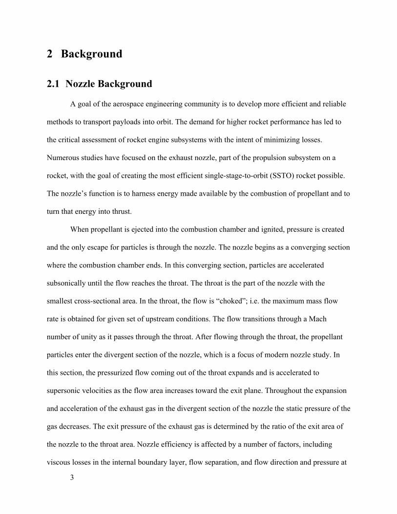
Figure 1: A Dual-Bell Nozzle [Copyright ©Nasuti, F., Onofri, M., & Martelli, E., 2005 [4]]
Dual-bell nozzles have been explored as a possible solution to maximizing efficiency at
high altitude while avoiding dangerous side loads at low altitudes. A dual-bell nozzle differs
from a conventional nozzle in that it has two distinct contours as opposed to one between the
throat and exit. A dual-bell nozzle consists of a base contour that is separated from the extension
contour by an inflection in the wall (see Figure 1). The effective cross sectional “exit” area of the
base nozzle is the area at the wall inflection. This area can be manipulated such that an effective
exit pressure for this section is matched to a relatively low-altitude pressure condition. The
inflection acts as a separation point and the separated flow is contained in the additional
axisymmetric area given by the extension contour. By controlling the separated flow, side loads
can be mitigated at low altitudes. As the rocket’s altitude increases, the flow re-attaches to the
wall of the extension due to decreasing ambient pressure. The exit area of the extension section
of the nozzle is sized for high altitude operation, thereby reducing efficiency losses due to under-
expansion. The dual-bell nozzle is an altitude adaptive nozzle by having a wall inflection that
allows one nozzle to be matched to two different ambient pressures [2].
5
2.1.1 Advanced Nozzles
Nozzles constrain the flow of exhaust gases, transforming the energy from an expanding
gas traveling at high speeds into thrust. Nozzles can be divided into two primary categories:
Thrust Optimized Contour (TOC) and conical contour nozzles. The profile of a conical contour
nozzle is defined by the half angle size. The method to create a TOC nozzle starts with the
method of characteristics, which produces a bell shaped nozzle that follows streamlines within
the flow field of an expanding gas [5]. Throughout the nozzle, the gas follows the contours of the
walls, expanding through small expansion waves. However, the rate at which the flow area is
increasing decreases throughout the bell curve of the nozzle, which is done in order to ensure a
uniform, directed flow field at the exit plane to maximize thrust. The decreasing rate of change
of the area causes small compression waves to propagate within the flow in the form of mild
oblique shocks. The idealized method of characteristics insures the mutual cancellation of these
oblique shock waves and oblique expansion waves, and thereby minimizes the energy loss. Ideal
bell-shaped nozzles are impractical because they are usually too long (and therefore too heavy)
for most vehicles [5].
Compressed versions of the TOC nozzle, called Truncated Ideal Contour (TIC) nozzles,
were designed in order to increase the performance of different vehicles above that produced by
a conical contour. The length of these nozzles is specified as a fraction of the length of a conical
nozzle with a 15° half angle. A contour can be created once the length is chosen by using
methods including the Rao method of characteristics, or by using a Rao parabolic approximation
for a bell-shaped contour. The latter is called a Thrust Optimized Parabolic (TOP) nozzle, which
increases the thrust potential of a rocket while reducing the length [5].
6

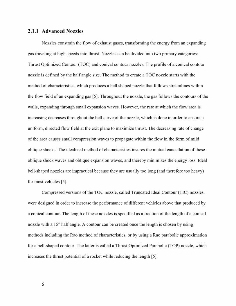
The Rao method of characteristics uses the method of characteristics to design nozzles. A
kernel flow, flow in the initial expansion region of the nozzle, is generated with the method of
characteristics for a wide variety of flow angles [1]. Next, the curvature of the throat is defined
and a nozzle curve is generated using other given parameters such as the area ratio and the length
of the nozzle. The contour is created by picking points on the flow field that result in a smooth,
theoretically shockless flow back to the throat. This process is rather complex, and the resulting
thrust optimized contour can only be defined by a coordinate list. Rao decided to approximate
this contour from the inflection point to the nozzle exit with a parabola.
Figure 2: Rao Parabolic Contour [Copyright Kulhanek 2012[6]]
Several problems have been identified with truncated contour nozzles, including a
tendency for flow separation to occur when operating at off-design conditions [7]. Flow
separation can occur in a TOP nozzle during the startup transient at sea level by the appearance
of a shock wave within the nozzle. The shock wave starts at the transition point from the circular
curve of the throat to the parabolic curve at the rest of the nozzle [8]. The shockwave within the
7

nozzle creates free shock separation (FSS) or restricted shock separation (RSS), which causes
dangerous side loading on the structure as well as hurting efficiency of the nozzle. In FSS,
(Figure 3a), the flow separates completely from the nozzle wall and continues as a free jet; this
occurs in over-expanded nozzles [8]. RSS (Figure 3b) causes the flow to separate as well, but it
reattaches to the nozzle wall downstream. This creates a separation bubble where a pocket of
flow is trapped within the nozzle. RSS is particularly harmful to a rocket due to the generation of
side loading from the shock separation and the potential of overheating caused by shockwave
interaction with the nozzle wall.
Figure 3: FSS vs. RSS within a conventional nozzle [Copyright © Hagemann and Frey 2008 [8]]
TOC nozzles are commonly used in rocketry and TOP nozzles were used on the Space
Shuttle Main Engine and RS-68 engine, and have experienced RSS and FSS during their use [8].
8
The design of a rocket nozzle is important because it dictates the performance of an engine,
which eventually determines the payload. TOP nozzles are a compressed, simplified version of
an ideal bell-nozzle created through the method of characteristics and experience FSS and RSS
when operating at off-design conditions. Another drawback for all of the different contoured
nozzles is that they are optimized for performance at one ambient pressure condition, which
correlates with one altitude. A number of altitude compensating nozzle concepts, such as the
dual-bell nozzle, have been proposed to achieve better performance over the entire flight of a
SSTO rocket.
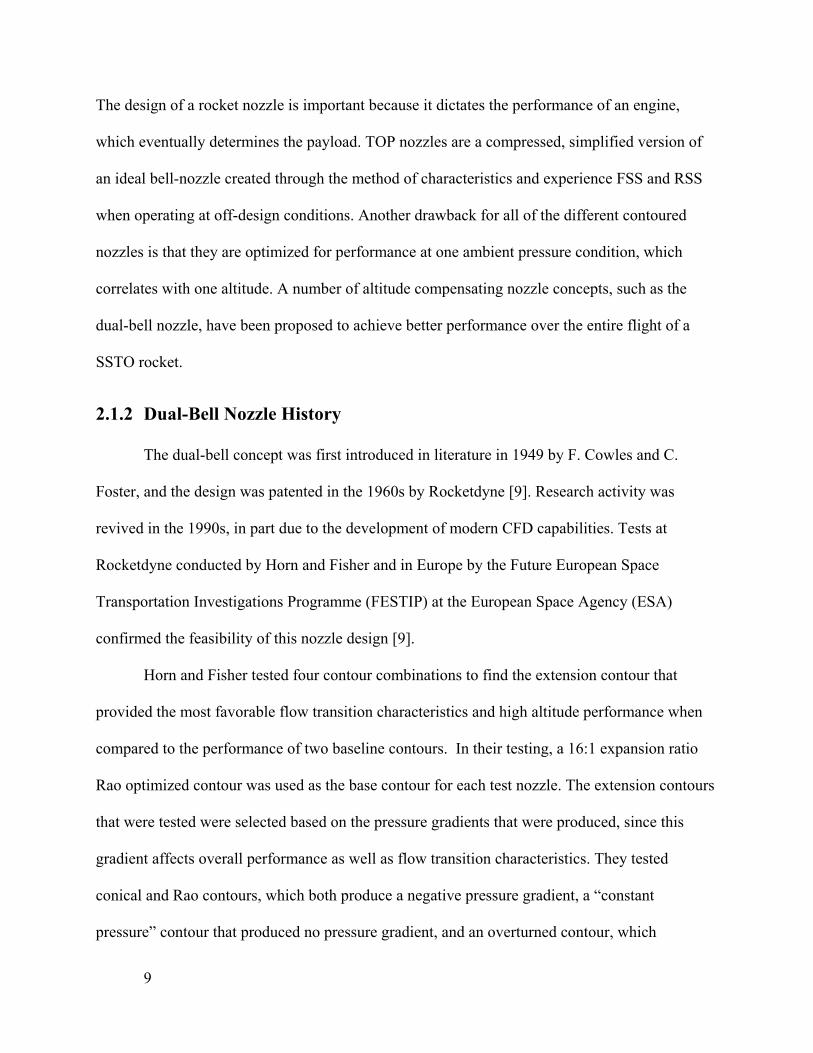
2.1.2 Dual-Bell Nozzle History
The dual-bell concept was first introduced in literature in 1949 by F. Cowles and C.
Foster, and the design was patented in the 1960s by Rocketdyne [9]. Research activity was
revived in the 1990s, in part due to the development of modern CFD capabilities. Tests at
Rocketdyne conducted by Horn and Fisher and in Europe by the Future European Space
Transportation Investigations Programme (FESTIP) at the European Space Agency (ESA)
confirmed the feasibility of this nozzle design [9].
Horn and Fisher tested four contour combinations to find the extension contour that
provided the most favorable flow transition characteristics and high altitude performance when
compared to the performance of two baseline contours. In their testing, a 16:1 expansion ratio
Rao optimized contour was used as the base contour for each test nozzle. The extension contours
that were tested were selected based on the pressure gradients that were produced, since this
gradient affects overall performance as well as flow transition characteristics. They tested
conical and Rao contours, which both produce a negative pressure gradient, a “constant
pressure” contour that produced no pressure gradient, and an overturned contour, which
9

produced a positive pressure gradient. They concluded that a constant pressure contour extension
provided the most beneficial combination of flow characteristics over the course of a SSTO
flight. However, they also demonstrated that real dual-bell nozzles fall short of the theoretical
optimum due to losses sustained from aspiration drag, earlier-than-ideal flow separation, and a
non-optimal contour for high altitude flight. Even with these additional losses, Horn and Fisher
found that a dual-bell nozzle could provide enough thrust to carry 12.1% more payload than a
conventional nozzle of the same area ratio [9].
P. Goel and R. Jensen performed the first numerical analysis of dual-bell nozzles, which
was published in 1995 [10]. Throughout the 2000s, several numerical and experimental studies
of dual-bell nozzles were conducted in the United States and Europe [2]. Modern studies
typically focus on optimizing particular design parameters of the dual-bell concept, such as
relative length of the extended section [9] and the ideal contour for the extended section [3].
2.1.3 Nozzle Comparisons
Conical contour nozzles are the most simple and, historically, the most commonly used
nozzle profile. These nozzles are characterized by a uniform profile from the throat to the exit
plane. They are simple in design and the least demanding to manufacture, but they have far from
ideal flow characteristics. The flow field is 2-D at the exit plane because of the constant, sloped
contour. This reduces the nozzle’s overall efficiency because the exhaust gas exits the nozzle
with a normal velocity component. In comparison, the exhaust gas in the ideal plume has only an
axial velocity component, resulting in an exhaust jet where all the momentum flux produces
useful thrust [1].
TIC nozzles are designed to produce a virtually unidirectional exhaust profile. The walls
of this contour curve near the throat region, but become nearly straight in the flow direction
10

towards the exit plane. To fully achieve the goal of unidirectional exhaust flow (i.e. an ideal
contour nozzle), the length of the nozzle must be equal to approximately 50 times the radius of
the throat. If this length was shortened and the flow forced to straighten out more rapidly, then
the exhaust speed of the gas, as well as the overall efficiency, would be lower. While a nozzle of
these dimensions would eliminate the losses due to non-axial flow divergence, its weight would
be impractical for flight. Thus, the truncated ideal contour nozzle is optimized to provide the
most unidirectional flow possible for a given constraint, such as expansion ratio, while
constraining the overall size and mass [1].
TOC nozzles are very similar in shape to truncated ideal contour nozzles: they are curved
near the throat and become increasingly straight in the flow direction. The main differences are
that a thrust optimized contour nozzle is curved more sharply near the throat, which corresponds
to a greater initial expansion of the flow, and it has a higher wall angle that turns the flow more
suddenly [1].
TOP nozzles are a skewed parabolic approximation of TIC nozzles. A geometric
discontinuity where the circular arc of the throat meets the parabolic arc produces an internal
shock that increases the wall pressure at the exit plane. The TIC nozzle is slightly more efficient
than a TOP nozzle, but the slightly higher wall pressure of the latter at exit offers a significant
overall advantage in that it can help avoid destructive side loads that are the result of highly
over-expanded nozzles at low altitudes [1].
11

Table 1: Comparison of Nozzle Contour Types
Nozzle Name Acronym Key Features
Conical N/A Straight walls from throat to exit
Incomplete flow turning
Truncated Ideal
Contour TIC
Curved walls near throat transition to nearly straight
walls near the exit
Virtually complete flow turning
Shortened version of the method of characteristics
Thrust Optimized
Contour TOC
Curved walls near throat transition to nearly straight
walls near the exit
More sudden transition than TIC
Virtually complete flow turning
Thrust Optimized
Parabolic (Rao) TOP
Parabolic approximation of TIC
Higher wall pressure at exit reduces risk of side loads
A dual-bell nozzle has three characteristic geometric features: an inner base nozzle
contour, a wall inflection, and an outer extension nozzle contour. At low altitudes, exhaust gases
expand in the base nozzle and separate at the inflection point, making the area at the inflection
point the effective exit area during this mode of operation. By having controlled, axisymmetric
flow separation, side loads are less of an issue than in conventional nozzles because the
separation point cannot fluctuate when the nozzle is under-expanded. As the rocket altitude
increases, ambient pressure decreases and the exhaust gases need a larger expansion ratio to
match, or approach, the ambient conditions. During this operational phase, the flow is attached to
the wall of the extension nozzle, and the whole exit area of the nozzle is used. Because of this
second section of the nozzle, the flow is not as under-expanded as it would be for a conventional
nozzle with the same area ratio as the base nozzle contour. Thus, the dual-bell nozzle achieves
improved high altitude performance over single-bell nozzles [2]. Additionally, dual-bell nozzles
12

have the unique benefit among altitude compensating nozzles of having no moving parts. The
controlled flow separation and mid-flight change in effective exit area is achieved only through
the geometry of the wall inflection. The extendable nozzle is another altitude compensating
nozzle that, similar to the dual-bell nozzle, uses varying effective exit area to improve flow
characteristics over a variety of ambient pressures. Unlike the dual-bell, though, the extendable
nozzle utilizes a deployable extension section that is actuated to move down over the base nozzle
and form the second contour of a dual-bell-like shape at a specific ambient pressure. The
disadvantage of an extendable nozzle is the additional weight and complexity that accompanies
the moving section of the nozzle. This makes the dual-bell nozzle a top contender among altitude
compensating nozzles because that translates to increased reliability, easier manufacturing, and
lower weight [2].
2.2 Application
The dual-bell nozzle for this project is being designed for a cube-satellite (CubeSat) launch
vehicle called Nanolaunch 1200. Several NASA centers and the Department of Defense (DoD)
as well as eleven universities support the project, which is being overseen by Dr. Jonathon Jones
from the Marshall Space Flight Center. The purpose of the Nanolaunch 1200 is to place a 3-U
(standard volume) CubeSat into low Earth orbit (LEO) for $1.2 million, with the goal to bring
this cost down to $250,000 within the next decade [11]. In order to accomplish this goal, the
contributors to Nanolaunch are both working together and competing against one another in
order to minimize the cost of the launch vehicle. A large part of this process involves using
commercial off the shelf (COTS) hardware combined with 3-D printing, also called additive
manufacturing. Nanolaunch 1200 is composed of four stages using a Black Brandt sounding
rocket for the first stage, a Nihka second stage, and two upper stages which are currently under
13

development [11]. The dual-bell nozzle in this project is being designed for possible future use
on the first stage. The Black Brandt sounding rocket uses the VC Mk 1 motor (Magellan
Aerospace/ Bristol Aerospace Ltd. of Canada), has an exit plane diameter of 17 inches, and is
210 inches tall [12]. The motor uses solid propellant, has an average chamber pressure of 1500
psi, and will be fired to propel the vehicle up to 20 km [11].
Nanolaunch 1200 will be valuable for DoD and commercial customers for a number of
reasons. The DoD applications mainly involve the need to acquire information or set up a
satellite while in a hostile territory. Currently, CubeSats are launched as secondary payloads on
large rockets with large and expensive primary missions, and consequently are limited to the
main missions’ constraints and schedules. Nanolaunch will be useful because CubeSats will not
need to wait for an upcoming launch to complete their missions [11]. Commercial customers will
benefit from Nanolaunch by receiving affordable access to LEO and having ridesharing
constraints removed from the CubeSats. They will be able to have an onboard propulsion system
and fewer restrictions as to when and where they launch.
The dual-bell nozzle being designed for this project is a proof of concept design to show
that the dual-bell contour can effectively delay flow separation through the flight of the Black
Brandt and increase the overall performance of the engine. This nozzle could help Nanolaunch
accomplish its goal to reduce costs by improving the specific impulse (Isp) of the first stage
motor averaged over its ascent trajectory.
2.3 Schlieren Imaging
Schlieren imaging, named after the German word for “streak,” is an optical technique for
studying inhomogeneous media. Robert Hooke developed the foundations of this technique in
the 17th century. It was not until the 19th century that the technique was significantly advanced by
14

J. B. Leon Foucault, who introduced a knife-edge cutoff as part of optical testing. Around the
same time, August Toepler reinvented Hooke’s technique, introduced the name “schlieren,” and
made the first major developments of practical apparatus for schlieren imaging. He was also the
first to see the motion of shock waves using his schlieren technique. Since then, schlieren
techniques have been further developed for various applications, including aeronautical systems
development and supersonic flows [13].
2.3.1 Optical Principles
Schlieren imaging uses the property that light travels non-uniformly through density-
inhomogeneous media to allow one to visualize density gradients in flows. The refractive index
for gases is related to density by
1 = 1
where is the refractive index, is the Gladstone-Dale coefficient for the gas, and is the
density of the gas [13]. Since the refractive index changes in proportion to density, the light path
is angled away from its original direction based on the density gradient of the media. These
deflections are generally small, but can be focused through a lens and made visible to an
observer. The ray deflection angle is given by
= , = 2
where is the length along the optical axis z and is the index of refraction of the surrounding
medium. The light is deflected by this angle in both directions (positive and negative) from the
original direction. This is for gradients of refraction in the x-y plane with the z-axis being the
direction of propagation of undisturbed rays [13].
A very simple point source schlieren imaging system consists of a light source, two
lenses with a test section between them containing the schlieren object (object of interest for
15

visualization), a knife edge, and a screen to capture the schlieren image. The first lens collimates
the light from the source and the second refocuses the beam onto the screen after the schlieren
objects refracts the beam. The knife edge is placed at the focus of the second lens. Without the
knife edge, every beam of light directed one way would correspond to another one directed
exactly opposite, cancelling out the effect. The knife edge blocks half of the beams so that the
effect of the refraction can be seen on the screen [13].
2.3.2 Applications to Flow Regimes
In his 1877 experiments to prove that waves from sparks were supersonic, Ernst Mach
used schlieren photography, starting a long history of applying schlieren imaging to viewing
high-speed phenomena [13]. Schlieren systems are considered the standard for high-speed wind
tunnel flow imaging, making it a perfect optical technique for this project. Information about the
location and shape of shock waves, the location of boundary-layer separation, and areas of wave
interference can be seen qualitatively using a schlieren system. In some circumstances, some
quantitative data may be gleaned from schlieren visualizations [13]. In cold-flow testing of
scaled-down dual-bell nozzles by Nürnberger-Génin and Stark [14] and Stark et al. [15],
schlieren imaging was used to observe the transition behavior and flow evolution between the
two nozzle contours. In addition, Stark et al. used schlieren images to determine the transition
duration and the angle of tilt of the Mach disk in the nozzle [15].
16

2.3.3 Schlieren vs. Shadowgraph Techniques
Figure 4: A shadowgram (left) and a schlieren image (right) [Copyright © Settles 2001 [13]]
Shadowgraph imaging is very similar to schlieren imaging and is based on the same
principle of refraction through inhomogeneous media. There are several key differences
however; most notably, the fact that shadowgrams are just shadows, whereas schlieren images
are focused optical images. Shadowgraph methods do not require a knife-edge cutoff, and the
apparatus to produce shadowgrams is simpler and easier to use. The light intensity variations in a
schlieren image represent the light deflection angle, while in a shadowgram ray displacement due
to the deflection angle causes the light intensity variations (Figure 4).
Shadowgrams are generally less sensitive to smaller density gradients than schlieren
images, but are useful when visualizing turbulent flows and shock waves. However, when the
disturbances are weaker overall, schlieren images accentuate detail of the flow around the
schlieren object and have the added benefit of a one-to-one ratio between image size and object
size [13].
17

2.3.4 Schlieren System Types
The simple point light source schlieren system discussed above under Optical Principles
(2.3.1) is an example of a simple-lens type system. In addition, there are various lens-and-mirror
type systems and a variety of large-field systems.
Figure 5: Conventional Z-type system [Copyright © Settles 2001 [13]]
In the historical development of schlieren systems, lens-and-mirror systems were
developed after the success of Foucault’s knife-edge experiments. The most popular of these
systems is the Z-type system, which employs two mirrors that are tilted in opposite directions.
The schlieren object lies between the two mirrors (Figure 5). One of the advantages of this type
of system is that having a larger than the mathematically required minimum distance between the
two mirrors to accommodate the test section does not affect the image; therefore the optical
system will not constrain the test section size. In addition, when set up correctly, the two mirrors
cancel out some aberration effects. Other mirror-lens systems include the single-mirror
coincident system, the off-axis single-mirror system, and multi-pass systems [13].
18

2.4 Computational Fluid Dynamics
2.4.1 Flow Regimes
When performing fluid analyses, flows can be separated into three categories: subsonic,
transonic, and supersonic (and in some cases, hypersonic as well). At lower velocities (below
Mach 0.7) fluids are conventionally taken to be incompressible as they flow through a channel.
As flow speed increases, however, compressibility effects must be considered. Gases can have
very large density fluctuations in supersonic flow due to their molecular structure.
Figure 6: A body placed in incompressible and compressible flow [Copyright © Auld and Srinivas 2006 [16]]
Compressible flows have varying densities. Calculations for compressible regimes are
more complex than for incompressible regimes due to density changes, disturbances, shock
waves, and expansion fans. This can be seen in Figure 6 as a shock wave forms in front of the
disturbance within the supersonic flow. The shockwave results in a different velocity profile after
the shock than would exist if the shock did not form. When a supersonic, compressible flow
approaches an obstacle, a shock wave forms, resulting in significant changes in the flow
properties over very short distances (Figure 6).
19

2.4.2 Turbulence Models
Turbulent flows are unpredictable and difficult to model accurately. Figure 7 shows the
differences in boundary layer flow behavior for subsonic and supersonic conditions. While
laminar flow along a boundary layer can be considered uniform, turbulent flow behaves
erratically in the boundary layer. Computational turbulence models allow for appropriate
estimations of these flows, which is important for high-speed applications. These are models that
capture the viscous boundary layer by approximately describing the velocity profile.
Figure 7: Flow near boundary layer for laminar and turbulent flow [Copyright © NASA Glenn Research center 2000 [17]]
The most common models for aerospace applications are Reynolds-averaged Navier-
Stokes (RANS) and Large Eddy Simulation models, which are named for their governing
equations. These models are separated into subgroups based on the number of transport
equations needed to compute the model [18].
Algebraic or Zero-Equation models are typically no longer used as they rely only on the
Navier-Stokes equations. Without the use of additional transport equations, these models are
oversimplified for complex geometries. These simpler equations normally do not suffice, but
when they are appropriate produce accurate results [18]. One-Equation models require one
transport equation to be solved to model the turbulent viscosity. The Goldberg, Baldwin-Barth,
20

and Spalart-Allmaras are included in this group. Of these, the Spalart-Allmaras is the most
commonly used [19].
Two-Equation models require an additional transport equation, but result in more
accurate flow models. The most popular two- - -omega, and
Menter Shear Stress Transport (SST), a combination of the previous two equations [17 -
epsilon model is consi -omega
model is typically used along boundary surfaces [19].
Turbulence models are selected based on the complexity of the flow field and the regions
of most concern within the flow. For most supersonic flows, these regions are the inlet, outlet,
hard surfaces, and/or contours.
2.4.3 FEM vs. FVM
For computer simulation of flows, there are two primary numerical methods used to
model fluid mechanics: the Finite Element Method (FEM) and the Finite Volume Method
(FVM). For this project, FVM is the better method, as outlined below.
FEM is more commonly used in analysis of solids, but certain Computational Fluid
Dynamics (CFD) programs do use FEM, such as COMSOL Multiphysics [20]. Analysis using
FEM begins with the definition of a boundary condition problem, created by the researcher.
Next, the researcher, with the assistance of a computer program, creates a mesh by dividing the
area in question into sub-regions. The solver then analyzes the flow over each element
individually. However, each boundary between cells is consistent, which allows the program to
combine the results into a contiguous whole. This process is extremely expensive in terms of
computing power, as it requires many iterations and a very large number of equations [21].
However, it is possible to model the mesh in a way to reduce the number of equations needed if
21

high precision is not required [22]. FEM tends to be better suited for either solid modeling or
modeling in multiple physical models, such as a problem with large non-linear deformation of a
flexible element in a flow field or modeling fluid flows with electrical interaction.
FVM is the most commonly used numerical method for boundary condition problems.
One key difference between FEM and FVM is that the flux between elements in FVM is
conserved. This makes calculations involving flux (such as many fluid dynamics problems)
much easier to handle. The basic process of solving a problem using FVM begins with meshing.
Each of these cells is treated as a separate control volume and a set of conservation equations is
applied to the flow for that specific cell. These equations are then broken down into algebraic
expressions, which can then be solved by a computer program [22].
Having a clear problem statement is crucial to obtaining accurate and consistent results
while using either of these methods. Both methods are only useful if the results can be
interpreted, which is why most CFD programs have a post-processing visualization tool [22]. In
addition, it is possible to solve physically impossible problems with a CFD solver returning
physically impossible results. Great care must be taken with any results from a computer
program to ensure that they reflect reality.
2.4.4 Turbulence Model Comparisons
Turbulence is the bane of CFD modeling and of fluid dynamics in general. It is nonlinear
and resists linearization in complex flows, leading to chaotic solutions and suboptimal
estimations. Despite these difficulties, various models for turbulence have been developed with
varying degrees of success. As already mentioned in Section 2.4.3, there are four primary
options: the Reynolds Average Navier-Stokes Equations (RANS), Large Eddy Simulation (LES),
22

Detached Eddy Simulation (DES), and Direct Numerical Simulation (DNS). This project used
RANS, detailed in this section.
Direct Numerical Simulation (DNS) directly solves the Navier-Stokes equations for
turbulence at all scales [23]. This method is possibly the most accurate model of reality at the
cost of extreme complexity. As the Reynolds number increases, the number of equations and
computational memory needed rises rapidly. This means that for complex geometries, this
method cannot be used within a reasonable timeframe [23]. For these reasons, DNS is not a
method that is feasible for primary use in this project.
Large Eddy Simulation (LES) is a simpler method for modeling turbulence than DNS and
as such is more widely used. The basic process of LES is the filtering of the Navier-Stokes
equations using a low-pass filter [24]. The low-pass filter removes the smallest equations from
consideration, greatly simplifying the problem. An accurate simulation for turbulence can be
developed in a reasonable amount of time while still returning results that reflect the turbulent
flow on a large scale. While this method uses fewer computer resources than DNS, it is still a
computer-intensive process that requires further modeling beyond the initial meshing, as each
mesh region is broken into smaller regions. Considering this complexity, LES is not the ideal
method for this project.
Detached Eddy Simulation (DES) is closely related to LES and RANS: in fact, it can be
loosely described as a hybrid of the two systems. In areas where more detail is needed, a method
closely resembling LES is used; however, in areas where LES is either not needed or not useable,
RANS is used. Effectively, DES is the best of both methods, but this again comes with a large
drawback: computational complexity. According to Spalart, a full simulation of a complex body,
23

such as an aircraft, would require in excess of 1011 grid points [25]. This project is limited to less
than 107 grid points in Fluent and as such, DES is beyond the computational resources available.
The precursor and basic model for all of these methods is RANS. For this method, which
was first developed in 1883 by Osburne Reynolds [26], the unsteady terms in the Navier-Stokes
equations are averaged out. This greatly simplifies the equations and allows them to be solved
without a CFD solver. It is possible (if impractical) to solve these equations by hand, given
enough time. For this reason, RANS is the best fit for this project. However, there may be certain
scenarios where a more detailed solution is required. In these cases, one of the other methods can
be used for that specific region, similar to how DES operates. For example, the inflection point
and surrounding flow pattern may need a more detailed model of the turbulence for a realistic
flow.
Table 2: Comparison of Turbulence Modeling Systems
Turbulence Models Advantages Disadvantages
DNS Most detailed system Extremely complex
Very slow
LES Faster than DNS Computationally complex
DES Adjustable Computationally impractical
RANS Can be solved by hand Least amount of details
24

3 Methodology
The primary focus for this project was testing a dual-bell contour in the supersonic wind
tunnel and testing a hypothetical full-scale nozzle using Fluent. These results were then
compared to a similar conventional nozzle for each case. In addition, Fluent was used to simulate
the flow through the supersonic wind tunnel in order to assess the comparability of Fluent results
and wind tunnel results.
3.1 Supersonic Wind Tunnel
Several previous MQP groups contributed to the development and construction of the
supersonic wind tunnel that was used for the project. Three MQP groups between 2009 and 2013
contributed to the design of the wind tunnel, the current version of which was completed during
the 2012-2013 academic year. The wind tunnel is an intermittent indraft tunnel. To operate it, the
vacuum chamber to which it is attached is pumped down to approximately 50 milliTorr. When
the valve that isolates the system from the atmosphere is opened, the vacuum chamber draws in
ambient air through the wind tunnel core. The pressure gradient between the near-vacuum
conditions on one end of the tunnel and ambient conditions on the other, in combination with the
geometry of the tunnel, is sufficient to produce a supersonic Mach number in the test section
[27].
The wind tunnel has three components in addition to an air drier. The flange assembly
connects the core to the vacuum chamber and supports the weight of the whole system. The core
contains the test section, with the geometry necessary to produce a supersonic flow. This section
consists of upper and lower contours placed opposite each other and two sheets of clear acrylic
that serve as windows into the test section. The contours in the test section are intended to
25

approximate a 2-D flow. The final component is the valve assembly, which seals the system
from the atmosphere. These three components were designed to be modular [27]. Thus, the
original core, which was designed to produce a flow with a specific Mach number, can be
removed and replaced with another core possessing the desired geometry for the test of interest.
For this project, the cores replicate the cross-sections of a dual-bell nozzle and of a conventional
TOP nozzle.
3.2 Schlieren System
The Design and Construction of a Supersonic Wind Tunnel with Diagnostics MQP [27]
designed a schlieren system to visualize the density gradients in their wind tunnel test section.
Their setup has been adapted for use in visualizing the density gradients of flow through 2-D
approximations of various conventional and dual-bell nozzle contours for this project. They
chose and constructed a conventional z-type system for their project which consists of a light
source, a condenser lens, a slit, two mirrors, a focusing lens, a knife edge, and a screen (Figure 8)
[27].
Figure 8: Existing Schlieren setup.
26

The light source has an adjustable goose-neck support enabling the light to be easily
directed towards the condenser lens. It also has a knob to control the light’s intensity. The
condenser lens serves to collect what ambient light cannot be eliminated as well as light from the
light source and distribute it evenly through the rest of the system. The slit, which is 0.36” by
0.072”, is oriented vertically to work with a horizontally mounted knife edge. The two mirrors
have focal lengths of 200mm, which is sufficiently less than the design distance between them,
which prevents them from interfering with each other. The focusing lens, placed within the focal
length of the second mirror, reduces the resulting image to a smaller area without compromising
its quality. The knife-edge is mounted horizontally on a vernier stage for fine adjustments of its
position to adjust image contrast. The screen consists of photo paper held flat on a mounted
clipboard. The components of the z-system are discussed by Bugden et al. in Design and
Construction of a Supersonic Wind Tunnel with Diagnostics [27].
One of the key advantages of the schlieren setup is its independence from the wind tunnel
and vacuum chamber assembly. The schlieren system relies on precise alignment of mirrors and
lenses, so it is mounted separately from the wind tunnel and vacuum chamber to minimize
potential vibrational effects. The schlieren system is mounted on a custom table constructed of x-
channel; two acrylic shelves hold the z-system setup and the light source, and adjustable feet
account for floor irregularities [27].
The z-system itself is composed of three pieces of x-channel held together by adjustable
locking hinges. The mirrors are mounted on the center piece of x-channel. One side piece holds
the condenser lens, and the other holds the focusing lens, knife edge, and screen. Bugden et al.
[27] finalized the distance between the two mirrors and the angle of the side x-channels to the
27

center piece through an optimization process. The final parameters chosen were 15° angles for
each of the side rails and a distance of 800mm between the mirrors [27].
Furthermore, Bugden et al. [27] developed a detailed set-up and alignment procedure for
use during testing. This reduced the learning curve for using the system with this project.
Adapting the z-system to this MQP was relatively simple. The test sections manufactured for this
project are the same dimensions as the ones used last year, so the system does not need to be re-
optimized [27].
3.3 COMSOL vs. Fluent
COMSOL and Fluent are two tools that were considered for possible use with the CFD
portion of the project. Both are powerful tools for simulation but have different characteristics.
Fluent works within the ANSYS (ANSYS, Inc., Canonsburg, PA) simulation software package
whereas COMSOL Multiphysics contains a CFD software package. Both can import CAD
geometries, and both are able to generate a mesh from the drawings. COMSOL uses finite
element discretization [28], which can increase computational time, whereas Fluent uses a finite
-
stress turbulence models. Georgescu et al. [20] compared the computational fluid dynamics
solvers by using both Fluent and COMSOL to model flow over a NACA airfoil. The flow
domain contained an equal number of nodes, but due to the difference between finite volume and
finite elements, the number of cells was different between the two cases. The case that ran with
COMSOL took over 10 hours to converge, whereas Fluent took less than 25 minutes. The results
of the study showed that both tools produce similar results, Fluent, however, took less time to
converge. S. Kulhanek [6] designed a conventional Rao nozzle contour then modeled its
28

performance using Fluent. This provided a baseline contour type to use for the baseline nozzle
comparison for this project.
Fluent was chosen as the CFD tool used to model the dual-bell nozzle because it is based
on a finite volume discretization scheme, which will help minimize computational time as well
as capture supersonic flow features such as shockwaves. COMSOL is able to model shockwaves,
however, it has a tendency to attempt to smooth them out and blend their effects into the
surrounding flow. Fluent uses a two- equation model for turbulent flow based on the shear stress
turbulence [22]. This model effectively captures the characteristics of boundary layer flows and
separated flows; examining both is the primary focus of this project. Fluent also uses a several
scale resolving turbulence models including large eddy and detached eddy simulations (LES and
DES respectively). Furthermore, the embedded-LES option (E-LES) enables computation of the
LES solution in selected subdomains within unsteady flows and can be coupled with a Reynolds
averaged Navier-Stokes model. This form of coupling further decreases computational time
while still capturing key flow features.
3.4 Thrust Optimized Parabolic Contours
A TOP nozzle is constructed using three curves (Figure 9): an initial, large circle coming
from the combustion chamber to the throat, a smaller circle exiting the throat, and a parabola to
extend the approximated bell contour to the exit plane.
29
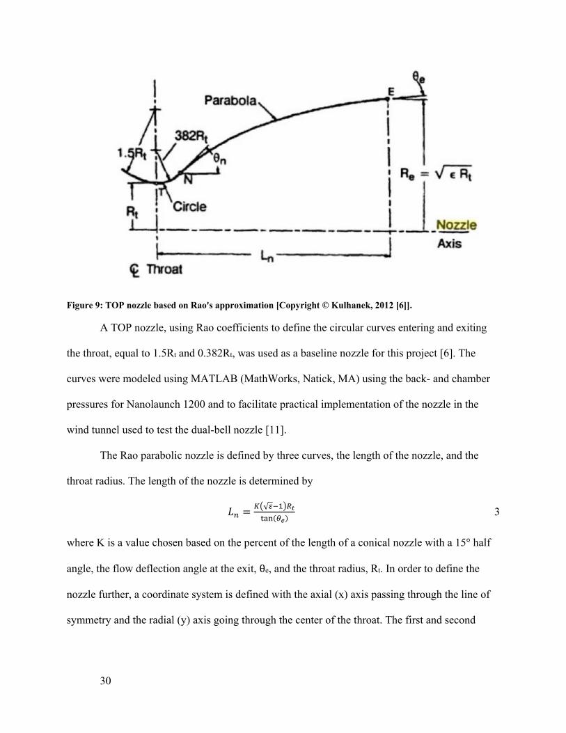
Figure 9: TOP nozzle based on Rao's approximation [Copyright © Kulhanek, 2012 [6]].
A TOP nozzle, using Rao coefficients to define the circular curves entering and exiting
the throat, equal to 1.5Rt and 0.382Rt, was used as a baseline nozzle for this project [6]. The
curves were modeled using MATLAB (MathWorks, Natick, MA) using the back- and chamber
pressures for Nanolaunch 1200 and to facilitate practical implementation of the nozzle in the
wind tunnel used to test the dual-bell nozzle [11].
The Rao parabolic nozzle is defined by three curves, the length of the nozzle, and the
throat radius. The length of the nozzle is determined by
= ( ) 3
where K is a value chosen based on the percent of the length of a conical nozzle with a 15° half
angle, the flow deflection angle at the exit, e, and the throat radius, Rt. In order to define the
nozzle further, a coordinate system is defined with the axial (x) axis passing through the line of
symmetry and the radial (y) axis going through the center of the throat. The first and second
30

curves define the entrance and exit of the throat of the nozzle, and are based on circular curves.
The first curve into the nozzle is determined by the equation:
+ ( ( + 1.5 )) = (1.5 ) 4
which can then be solved for y. Note the curve is defining the bottom half of the circle, and
therefore is negative.
= (1.5 ) + 2.5 5
The second curve begins at the throat where the derivative of both curves is equal to zero.
The second curve is also a circle defined by the equation:
+ ( ( + 0.382 )) = (0.382 ) 6
which leads to the equation for the second circle:
= (0.382 ) + 1.382 7
In order to ensure a smooth transition from the combustion chamber to the throat, there
needs to be continuity between the curve defining the combustion chamber and the entrance to
the throat. That is, the derivative for both points needs to be equal:
= tan( ) =( . )
8
where 1 is the angle at the start of the curve ( x = -0.0184 m ), and x1 is a function of the throat
radius and 1.
The curve leading from the combustion chamber to the throat curvature begins at x1,
which equals:
= 1.5 sin( ) 9
The equation of the parabola, curve 3, takes the form
= + + 10
31

and the coefficients are determined by the derivatives at the point where the circle from the
throat meets the beginning of the parabola, xN, and the length of the nozzle. To determine xN, the
angle, N needs to be defined, then the derivative of the second curve should be equal to its
tangent.
= tan( ) = ( . ) 11
This is then solved for xN.
= 0.382 sin ( ) 12
At xN, both the derivatives for the parabola and the circle have to be the same and both
have to meet. This leads to the following constraints for the coefficients of the parabola.
= + + 13
= tan( ) = 14
To complete the series of equations the exit of the nozzle is examined, where x is equal to
the nozzle’s length, Ln. Ideally, the flow should have been turned as close as possible to
horizontal by the exit plane, and the derivative of the parabola evaluated at Ln is used.
= tan( ) = 15
This completes the linear system of equations. In matrix form, the system is
2 1 02 1 0
1=
( )
( ) 16
which can then be solved for the coefficients.
32

3.5 Dual-Bell Nozzle Design
The dual-bell contour design adds a fourth curve to the conventional Rao design by
adding a second parabola to connect two Rao that share the same throat area, but are optimized
for different altitudes. The second parabola defines the second bell section and connects the two
contours thereby achieving a greater expansion ratio.
The dual-bell nozzle was defined similarly to the contour of the Rao nozzle, with the
same throat entrance and exit parameters as defined in equations 10 and 12. The parabola
coefficients for the first parabola were found using the same method as the Rao contour. Figure
10 shows a Rao nozzle contour optimized for two different altitudes (3.05 km and 16.97 km),
corresponding to two different ambient pressures (10.1 psi and 1.5 psi).
Figure 10: Rao Contours for different altitudes
A dual-bell nozzle connecting the two Rao nozzles, with an optimized design point for
altitudes of 3.05 km and 16.7 km is shown in Figure 11.
33

Figure 11: Dual-bell contour connecting two Rao contours designed for different ambient pressures
The coefficients of the second parabola were found using the inflection point, x=xM, the
inflection angle, M and the exit angle, e. As shown in Figure 11, the distance at xm is the
distance to the inflection point, and was defined using
= ( ) 17
where the K value KM was reduced to 0.7 in order to keep the overall nozzle a reasonable length.
Figure 12 shows a normalized dual-bell contour. It has equal sized axes in order to better
represent the actual nozzle’s shape.
34

Figure 12: Dual-bell nozzle with normalized axes
Figure 13: Dual-bell nozzle with labeled sections (axes scaled for clarity)
35

A parabola defines the second curve, and the coefficients were solved for using the same
derivative method used to make the first curve and the Rao contour. The system of equations to
solve for the coefficients of the second curve is:
2 1 02 1 0
1=
( )
( ) 18
where a’, b’ and c’ are the coefficients of the second curve. The full system definition is
provided in Appendix D.
36

4 Experimental Procedures
4.1 Setup and Experiments
4.1.1 Alignment and Focusing
The eight components of the schlieren system must be in specific locations with respect
to the other components in order to use it (Figure 8). The components are arranged in three
segments of the z-type system. The first segment begins at the light source, includes the
collimating lens and the slit, and ends at the first mirror. The second segment extends from the
first mirror to the second mirror, and is referred to as the test section of the schlieren system. The
third segment begins at the second mirror, includes the razor blade and the focusing lens, and
ends at the screen.
In order to obtain the best possible schlieren images, the components of the system must
be aligned very precisely. A good image should be circular in shape (if the mirrors are circular),
focused, and it should exhibit high contrast without being too dark. The location and orientation
of all of the components contribute to having a sufficiently bright image, but the slit has the most
direct effect. Placing the slit closer to the collimating lens increases the amount of light that
passes through it, and placing it further away from the collimating lens reduces this amount of
light. Ideally, the light beam that passes through the slit should be the same diameter as the first
mirror to maximize the brightness of the image while reducing light pollution.
The focus of the image is largely controlled by the focusing lens, which is the last optical
component that the light bean passes through before being projected on the screen. Ideally, this
lens should capture all of the light that passes by the razor blade. Thus, the optimal place for the
focusing lens is after the razor blade and anywhere within two focal lengths of the second mirror.
37

If this lens is placed further than two times the focal length of the second mirror, then light
would be directed onto the screen without being focused. This results in an unfocused image as
well as significant light pollution.
Finally, having high contrast is critical to obtaining useful images, and this quality is
largely controlled by the height of the razor blade. The focused light beam takes the shape of the
vertical slit that it passed through in the first segment, and thus the horizontal razor blade is ideal
for cutting off a portion of the light beam. The higher the razor blade, the more of the light beam
(which consists of both parallel and refracted light) gets cut off. The effect of this is that the
highest contrast images are also very dark, so a middle ground between brightness and contrast
must be determined while adjusting the height of the razor blade.
4.1.2 Updates to Existing Schlieren System
In order to obtain the best possible schlieren results, significant changes were made to the
existing schlieren system. The first change that was made was to add ball and socket mounts to
both mirrors between the mirror mount and the conversion piece that connects to the post. This
change allowed for easier alignment of the surfaces of the two mirrors with one another.
However, these mounts on the mirrors necessitated machining new posts for all of the
components to account for the height added to the mirrors and to keep the focal points of all
components on the same plane. The posts were made out of 4-inch long steel bolts that were
machined to the proper size using a lathe.
Next, specific components had to be improved. A bracket was machined to hold the light
source gooseneck in a specific location. The bracket is a cylindrical piece of aluminum with a
hole bored out along its length such that the end of the gooseneck can be inserted into the bracket
and then secured using a setscrew. The bracket is held up to the appropriate height by a threaded
38

aluminum post. By securing the light source, the proper alignment is much easier to achieve and
the system is much more resilient to minor disturbances than it was when the gooseneck was a
freestanding component.
The screen and the slit elements of the system also required improvement. These
components were originally made of materials that were not ideal for this application, so new
parts were made using opaque, white acrylic. Both the screen and slit were designed to be
freestanding so that their positions can be individually optimized based on the final alignment.
For the screen, the acrylic was sanded with a fine grit sandpaper to get a matte finish. This is
ideal because light pollution could reflect off a glossy screen and interfere with the image
captured by the camera. For the slit, the small section of a metal eraser shield previously used
was kept, but it was mounted on a piece of acrylic rather than construction paper so that the only
light that passes this component passes through the slit.
The system has an optimal alignment, and once that alignment is achieved, there is no
advantage to the ability to move individual components and having movable components puts
the system at risk for being misaligned in the future. Therefore it was determined that the system
would have to be removed from the original x-channel base and reconfigured using a solid
aluminum plate as the base. This decision was based on the difficulty of achieving a proper
alignment on the x-channel base. Once all of the new components were incorporated into the
system, the three segments of x-channel were detached from each other so that a new
optimization exercise could be carried out to determine the ideal distances and angles in the
system. This optimization exercise is detailed below in the Section 4.1.3, “Optimization and
Specific Setup.” After the alignment was optimized, the distances between components and the
angles between segments were used to design the optical plate.
39

The optical plate is a complex shape that was machined from a 36” x 24” x 1/4” plate of
aluminum. The geometry is a result of the alignment needed to obtain a schlieren image and the
physical constraints of the wind tunnel and vacuum chamber. The design for the layout of the
holes was made using SolidWorks (Dassault Systemes SolidWorks Corporation, Waltham, MA)
computer aided design software. Only holes for the posts that hold the light source gooseneck,
collimating lens, the two mirrors, and the focusing lens were machined into the plate. It was
determined that keeping the slit, razor blade, and screen free-standing would allow for finer
adjustment of the most sensitive component locations. Additionally, holes were placed at the
corners of the optical plate so that it could be raised or lowered as needed for use with the wind
tunnel. All the holes are size ¼”-20. After the SolidWorks design was complete, it was converted
into a design that could be read and produced by a machine using Esprit computer aided
machining software. Finally, the optical plate was manufactured using a CNC milling machine
located in the WPI Washburn shop. The plate did not fit on the schlieren table that was produced
by a previous MQP group, but a suitably larger table was found.
Figure 14: Solid model of optical plate
40

4.1.3 Optimization and Specific Setup
The first step to optimizing the system alignment was to align the two parallel segments
of the z-system. For the first of these, the segment with the light source, the components were
adjusted to concentrate the light hitting the first mirror. This both channels as much light as
possible through the test section (resulting in brighter images), and reduces light pollution. For
the other parallel segment, the section with the screen, the adjustments focused around the razor
blade, as its position needs to be precise in order to produce a schlieren image. The razor is
placed just behind the second mirror’s focal point and raised up so that it cuts off more than half
of the light beam. After the razor was positioned, the focusing lens was adjusted such that all of
the light that passes the razor blade is captured within the lens. Finally, the screen was adjusted
along the optical axis with respect to the focusing lens until a clear image appeared.
After the lengths of the parallel segments of the system were determined, the length of
the second segment (the test section) as well as the angle between the segments was varied so as
to maximize image quality. To determine the best arrangement, an optimization experiment was
conducted. Test section lengths of 80 cm, 90 cm, and 100 cm were tested, as well as angles of
15°, 20°, 30°, and 40°. Certain configurations were eliminated because they did not allot enough
physical space for the wind tunnel, which at its widest requires at least 12 cm of space in the
second segment without interfering with the components in either the first or third segments.
Table 3 summarizes the results obtained by imaging a heat gun using a number of
different configurations which vary the test section length and angle while keeping the test
section normal to the wind tunnel.
41

Table 3: Summary of Results from Optimization Exercise
Trial Test Section Length (cm)
Angle (°)
Space for Wind Tunnel Width (cm)
Photographic Results Comments
1 80 15 9.49 N/A Too Small to fit wind
tunnel
2 80 20 11.40 N/A Too Small to fit wind
tunnel
3 80 30 16.78
Good contrast, wind
tunnel will fit, but with
less clearance than other
configurations, good
focus
4 90 15 19.49
Non-circular image,
moderate contrast
5 90 20 21.40
Non-circular image, low
contrast
6 90 30 26.78
Very good contrast,
allows enough space for
wind tunnel, good focus
42

7 100 15 29.49
Non-circular image,
blurry focus, low contrast
8 100 20 31.40
Lens height had to be
adjusted, good contrast,
leaves room for wind
tunnel, focus slightly
blurry
9 100 30 36.78
Lens height had to be
adjusted, good contrast,
leaves room for wind
tunnel, focus slightly
blurry
Based on the results of the optimization, the following configuration provided the best
resulting images and thus it was the basis for the design of the optical plate:
Table 4: Optimal Configuration for Schlieren System
Components Distance (cm) Angle from test section (°)
Light to Collimating Lens 3 30
Collimating Lens to Slit 4
Slit to First Mirror 18.5
First Mirror to Second Mirror 90 N/A
Second Mirror to Razor 24 30
Razor to Focusing Lens 8.5
Focusing Lens to Screen 15
43

4.1.4 System Validation Experiments
To validate the chosen configuration, a number of phenomena were imaged using the
system in its optimal configuration. The phenomena create density gradients in the surrounding
air either through heating or by creating a relatively fast jet of gas (adjacent to still air) using a
can of compressed air. Combinations of phenomena were also imaged. These images were
modified using Windows Live Photo Gallery software (Microsoft Corporation, Redmond, WA)
to adjust the brightness and contrast of the images as necessary. During modification, the
brightness was increased slightly because the best images, which are obtained with the razor
blade blocking half of the refracted light, tend to be very dark. Increasing the brightness makes
the flow structures easier to see. For the same reason, the contrast of the images was increased
slightly. Both of these modification processes are suitable for schlieren images because they
change properties of the whole image rather than only a part of it. Therefore, the flow properties
that can be discerned in the image are not altered through the image modification, but simply
made easier to see. Image enhancement that changes the appearance of the flow with respect to
the whole image as opposed to changing the whole image itself is not suitable for qualitative
analysis of schlieren images.
44

Candle
Figure 15: Schlieren image of a candle flame
Figure 15 shows the top of a candle flame where the density gradients produced by the
uneven heating of air in the test section transition from smooth, gradual gradients to more
random and sudden gradients in the air further above the candle. In the schlieren system, the
image appears inverted on the screen, but for ease of analysis, all photos in this paper have been
rotated to reflect the orientation of the phenomena as it was being imaged.
45

Heat Gun
Figure 16: Schlieren image of a heat gun
The lip of the heat gun obstructs part of the light beam in the test section, thus producing
a non-circular image. The heat gun not only produces density gradients that can be viewed with a
schlieren system, but it also produces streak-like regions of similar density gradients, as can be
seen in Figure 16.
Compressed Air
Figure 17: Schlieren Image of a Jet of Air
46

The compressed air produces a density gradient due to its velocity rather than
temperature, as with the other phenomena in this study. The density gradients that will be
observed in the wind tunnel will similarly be produced by the high velocity flow of air. The
velocity of the flow is not imaged, but the differences in densities that are produced by the
different relative velocities in the test section are what produce the dark and light areas in the
image.
Interference of candle and compressed air
Figure 18: Schlieren image of the interference between a candle flame and a jet of air
Figure 18 shows the region directly above the flame of a candle where the density
gradients would normally transition from being smooth and gradual to more erratic. This
transition is further facilitated by directing a flow of high velocity air at the same region, thus
producing the sudden and rapid gradients indicated by the distinct light and dark areas in the
figure.
47

Non-interference of candle and compressed air
Figure 19: Schlieren image of non-interference between a candle flame and a jet of air
Figure 19 shows two phenomena that are both in the test section of the schlieren system,
yet not interfering with each other because they are placed approximately 15 inches away from
one another in this image. This image demonstrates that the system has the sensitivity to detect
density gradients anywhere along the length of the test section.
4.2 Manufacturing Test Nozzles
New contours for the supersonic wind tunnel designed by a previous MQP group [27] for
use with the vacuum chamber were created to test the viability of the dual-bell nozzle contour,
and to compare the flow structures with those found in a conventional TOP nozzle design. The
nozzle contour designs were scaled to fit the dimensional constraints of the existing test section.
48

4.2.1 CAD Nozzle Modeling
The previous MQP group [27] provided the SolidWorks CAD models for the basis of this
project’s supersonic wind tunnel test section design. The parts from the previous test section
were adapted to this project’s nozzle designs. The previous test section had a single piece that
served as both the nozzle contours as well as the brackets connecting to end plates and acrylic
windows (Figure 20). Last year’s group started designing a new configuration for the test
section, in which the contours would be separated from the brackets, so that the contours could
be removed and replaced with different contours while using the same brackets (Figure 21). The
contour is only connected to this bracket via three bolts, and the entire piece is within the O-ring
seal to prevent leaks from arising due to the separation of these two pieces. This year’s project
finished designing and constructing this new test section design, which allows the wind tunnel to
be more modular. The nozzle contours, designed for the first stage of the Nanolaunch vehicle,
must be scaled down to fit the wind tunnel test section size. The contours for the Fluent analysis
and actual application are on the order of half a meter to a meter in scale, while the test section is
on the order of inches. In addition to the required dimensional scaling, the contour was also
modified to adapt an axisymmetric flow channel (i.e. the nozzle) to the 2-D rectangular geometry
inherent to the test section.
49

Figure 20: SSWT CAD model from the 2013 MQP [27]
Figure 21: CAD model of new set-up with dual-bell contours
4.2.2 Manufacturing Constraints
The largest constraint in designing and manufacturing the nozzle contours was the small
size of the wind tunnel test section. The size of the throat is governed by the design Mach
number for the contour, but due to available machining capabilities, there is a limit to how
50

accurate the throat can be machined. The size of the test section itself limits how large the exit
area can be, which changes how the throat area affects the overall nozzle design. This means that
the area ratio may not be the same as it is for the original Fluent design. The manufactured
contour was also limited in length in order to be able to use the same test section configuration as
the previous MQP [27]. However, the assembly and disassembly of the wind tunnel test section
was greatly simplified with the new parts. One set of contours can be replaced with another
without any modification of other parts of the wind tunnel test section.
4.2.3 Manufacturing Processes
Our test setup is based on work done by previous MQP groups; however, many
components could not be reused for various reasons. The ball valve and mounting flange sections
were reused from the supersonic wind tunnel, but most parts in the test section had to be
machined for this project.
51

Figure 22: Wind tunnel set-up
Ball Valve
Test Section
Mounting Flange
52
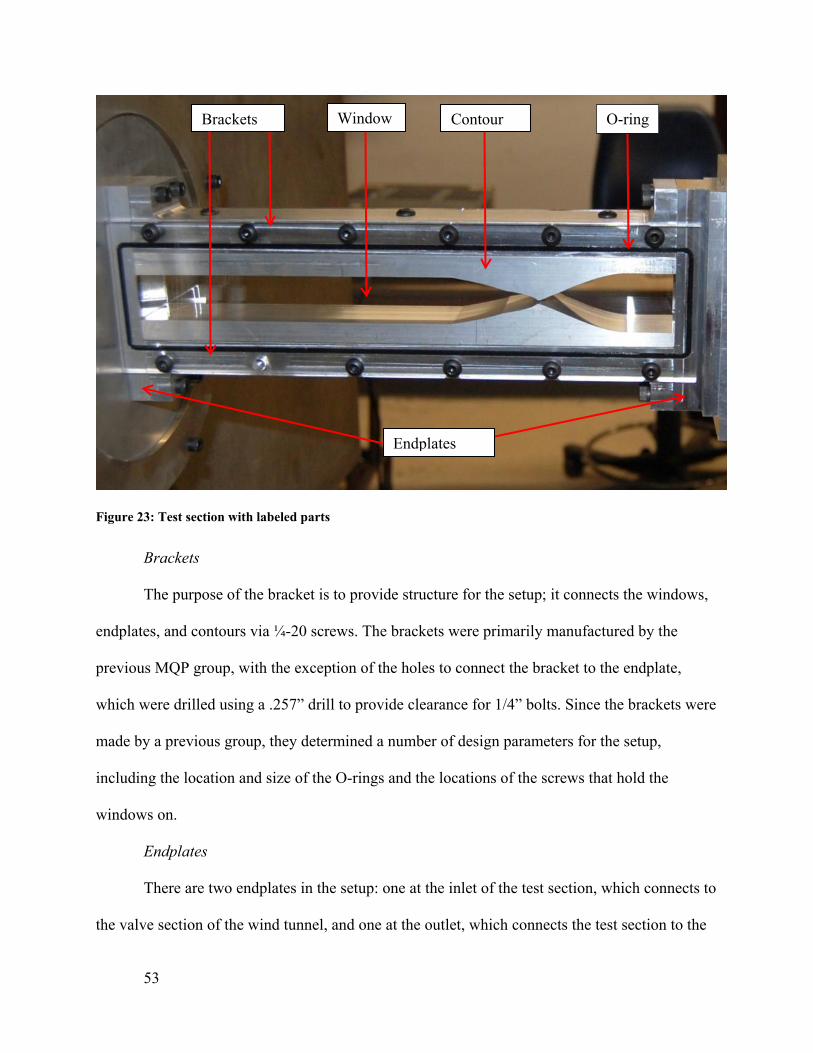
Figure 23: Test section with labeled parts
Brackets
The purpose of the bracket is to provide structure for the setup; it connects the windows,
endplates, and contours via ¼-20 screws. The brackets were primarily manufactured by the
previous MQP group, with the exception of the holes to connect the bracket to the endplate,
which were drilled using a .257” drill to provide clearance for 1/4” bolts. Since the brackets were
made by a previous group, they determined a number of design parameters for the setup,
including the location and size of the O-rings and the locations of the screws that hold the
windows on.
Endplates
There are two endplates in the setup: one at the inlet of the test section, which connects to
the valve section of the wind tunnel, and one at the outlet, which connects the test section to the
Endplates
Brackets Window Contour O-ring
53

flange. The purpose of the endplates is to transition the channel size, which is 1” x 1.25” in the
valve section, 1”x1.5” in the test section, and 1”x1” in the flange. The endplates were
manufactured using a CNC machine with a 1/2” end mill, 1/4” ball mill, a .257” drill bit, and a
1/8” end mill.
Fixture plate
While not a part of the final assembly, the manufacturing of the fixture plate was a key
step towards machining the contours (Figure 24). The fixture plate is designed to hold the blank
from which a contour is made to the machine during the manufacturing process. This part was
made on a CNC machine using a 1/2” mill, a 3” face mill, a 33/64” drill bit, a .257” drill, and a
¼” end mill.
Figure 24: Fixture plate attached to CNC machine
54

Figure 25: Dual-bell contour during machining process using the fixture plate
Contours
The geometry of the contours was first created using Matlab, and the resulting curves
were imported to SolidWorks. The final design of the nozzle was made using the equation driven
curve feature. An attempt was made to use imported numerical points to define the curve, but
this method did not produce a high enough resolution. These CAD designs were then transferred
into CAM files that could be read by a CNC machine. The contours began as 1” x 1.5” aluminum
stock that was cut down to approximately 12.25” in length using a horizontal band saw. These
pieces were then milled down to 12” on a CNC machine using a ½” end mill. In the same
process, a 0.201” drill bit was used to make the three holes that were later used to connect the
55

blank to the fixture plate and then to connect the completed contour to the bracket in the test
setup. With the blanks screwed to the fixture plate, the machining of the contours was
accomplished with a CNC machine using a ½” end mill and a 1” end mill. The tolerance of the
CNC machine used was 6/1000”.
Windows
The windows for the test section were originally made from ¼” clear acrylic. The
dimensions and hole pattern were determined using the CAD model of the brackets. Once the
design was complete, it was machined using the laser cutter. However, during testing it was
discovered that fine, spider cracks formed around the holes in the acrylic when it was screwed
down to the brackets. To alleviate this problem, ¼” clear polycarbonate, which is stronger and
more resilient under compression than acrylic, was selected as the material to be used for the
final design. The same CAD model was used to produce the polycarbonate windows, but they
could not be produced on the laser cutter. Polycarbonate absorbs infrared radiation, so using a
laser would result in poor edge fidelity, discoloration, and possibly burning of the material.
Instead, the windows were machined using a CNC mill.
O-rings
The O-rings were made using 0.1” diameter Buna-N (nitrile) O-ring stock and Loctite
404 super glue to splice the ends together. Because the super glue becomes very hard when dry,
the joining surfaces at the ends of the O-ring stock were cut such that no cross section would be
entirely hardened super glue, which would impede the compression of the O-ring and cause a
leak (Figure 26). The O-ring stock was cut using a razor blade. Once the stock was cut to size
and the ends cut to form a half-lap joint, a small amount of super glue was applied to one of the
56

joining surfaces. The joining surfaces were then brought together and held for approximately ten
seconds until the glue dried.
Figure 26: Lap joint used for O-ring joining surfaces
4.3 Testing Nozzles in Supersonic Wind Tunnel
Once the new supersonic wind tunnel test sections and the improvements to the schlieren
system were completed, the entire system was tested to see the effects of different contours on
the flow. The schlieren system had been tested with a candle and a jet of compressed air to
ensure that it worked properly, but the wind tunnel set-up could only be tested when connected
to vacuum chamber. Both the dual-bell and Rao nozzle contours were tested to see how the flow
structures differed between the two nozzle types and compared to the ANSYS Fluent
simulations.
57

4.3.1 Test Set-Up
The test section is connected to the vacuum chamber via a mounting flange, and there is a
ball valve at the other end of the test section, which is opened to start the test. The schlieren
system sits on a table under the wind tunnel test section, with the optical elements mounted so
they are centered on a plane that intersects the test section. The entire set-up can be seen in
Figure 27. The schlieren system plate can be shifted on the table to focus on different areas of the
test section.
Figure 27: Test Setup
The first tests run with the wind tunnel test section were to ensure that the set-up was
working correctly. Leaks are a major concern for this project, because they prevent the vacuum
chamber from pumping down. The first time the vacuum chamber was pumped down with the
58

new supersonic test section, leaks were immediately noticeable by a distinct hissing sound.
Applying vacuum grease to the O-rings helped prevent some of the leaking; however, a small
leak was still present, located between the brackets and the end plates of the test section
assembly. This was sealed with silicone caulk. To ensure a solid seal, the brackets and end plates
were disassembled and cleaned thoroughly before applying caulk to the entire face. The sealant
was chosen to be airtight, but removable with a solvent so that the system could remain modular
and allow for other contours to be tested. After applying the adhesive, the test section assembly
was sufficiently sealed for testing.
Once the system was sealed enough for the vacuum chamber to pump down, the actual
tests of the contours began. Each test begins by ensuring the vacuum chamber is pumped down,
aligning the schlieren system so that the section of interest is in the field of view. One person
captures schlieren images of the flow throughout the test. The image capturing starts when the
valve is opened, and ends when the pressure in the vacuum chamber reaches atmospheric. Tests
were conducted at various points along the length of the test section to see how the flow differed
in and downstream of the nozzle.
4.3.2 Interpretation of Images
Images were taken throughout the duration of each test at a single location along the test
contour. Multiple tests were conducted with both the dual-bell and Rao contours to image the
flow at various points within and downstream of the nozzle (i.e. into the test section of the wind
tunnel). The schlieren images were analyzed to determine the flow structures in the test section.
Schlieren images show density gradients in a flow, so sharp changes in density appeared as dark
lines in the schlieren images, while areas of constant pressure appeared bright. Examining the
images over the course of one test shows how the flow changes as the back pressure increases
59

throughout the test. Multiple tests were conducted with each set of contours to confirm the
repeatability of the flow structures captured with the schlieren images. The flow structures
revealed in the images were compared to structures simulated with ANSYS Fluent to assess
similarities and differences.
4.3.3 Rao Image Analysis
In several tests using the Rao contours, two flow features were imaged: A normal shock,
and a series of boundary layer flow structures. A normal shock, which appeared in the nozzle
immediately at the beginning of the test, consisted of a thin, dark curved line followed by a light
region. This shock moved upstream as the backpressure increased. The normal shock was only
visible for approximately the first thirty second of the test. During this time, it moved upstream
through the nozzle.
Figure 28: Normal shock with Rao Contours
As the normal shock moved upstream through the nozzle and approached the throat at the
beginning of the test, it began to assume a more angular geometry as opposed to curved shape.
60

The leading edge of the shock remained normal to the flow, but the tips became parallel to the
nozzle contour. Very shortly after taking on this angled form, the normal shock dissipated.
Figure 29: Normal Shock with Angled Shape in Rao Contours
Immediately following the dissipation of the normal shock, a series of boundary layer
flow structures began to appear. Each of these structures consisted of a dark streak, which
indicates a rapid change in density, followed by a small, nearly circular light region, which
indicates a negligible change in density in that region.
61

Figure 30: Early Development of Boundary Layer Structures
The first boundary layer structures that formed were relatively spread out. As the test
went on and the back pressure increased, the structures moved upstream towards the throat.
Figure 31: Advanced Development of Boundary Layer Structures
62
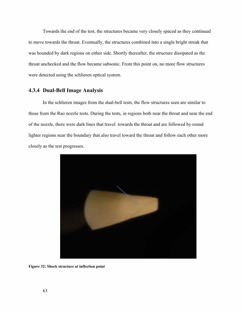
Towards the end of the test, the structures became very closely spaced as they continued
to move towards the throat. Eventually, the structures combined into a single bright streak that
was bounded by dark regions on either side. Shortly thereafter, the structure dissipated as the
throat unchecked and the flow became subsonic. From this point on, no more flow structures
were detected using the schlieren optical system.
4.3.4 Dual-Bell Image Analysis
In the schlieren images from the dual-bell tests, the flow structures seen are similar to
those from the Rao nozzle tests. During the tests, in regions both near the throat and near the end
of the nozzle, there were dark lines that travel towards the throat and are followed by round
lighter regions near the boundary that also travel toward the throat and follow each other more
closely as the test progresses.
Figure 32: Shock structure at inflection point
63

For the dual-bell case, the dark lines, corresponding to shock structures, form at the
inflection point (Figure 32). This test was focused on the sections of the nozzle further
downstream in order to see the behavior in the vicinity of the inflection point
Figure 33: Boundary layer flow features
As the test continues the first round lighter region forms at the inflection point along the
boundary directly downstream of the shock. The beginning of the lighter region’s formation can
be seen in Figure 32, and the fully developed flow feature can be seen in Figure 33. Also visible
are more of these boundary layer features, which continue develop at the inflection point and
further towards the downstream end of the nozzle throughout the test. These flow features travel
upstream toward the throat, following the shock.
64

Figure 34: Throat region shock and boundary feature
Figure 34 shows the shock and boundary layer feature closer to the throat in a test run
that focused on the throat region. As the test continues, the shock is swallowed and the boundary
features become closer together as they travel towards the throat. This phenomenon can be seen
in Figure 35. At some point in the test, all of the remaining boundary flow features are
swallowed by the throat as pressure differential decreases. Eventually the throat unchokes and
the flow becomes subsonic for the remainder of the test.
Figure 35: Series of boundary flow features
65

5 Numerical Simulation
5.1 Mesh Generation
5.1.1 Full-Scale Nozzles
The mesh for both the dual-bell and the Rao contours was generated using the ANSYS
Workbench mesh generator. The meshed region covers the nozzle and a significant downstream
area. The area downstream of the exit enables the solver to fully develop the flow within the
nozzle, and enables visualization of different flow structures, such as Mach diamonds and
expansion or compression waves that occur downstream of the exit plane. Figure 36 shows the
fully defined Rao nozzle contour with the downstream section.
Figure 36: Rao nozzle mesh with downstream section
This mesh is dependent on properly labeling and joining edges within the “geometry”
option within Workbench. While checking the imported geometry from SolidWorks, label the
inlet, outlet, nozzle walls and nozzle exit plane by inserting a “named selection” on each of those
66

areas. This informs Fluent where to define boundaries and makes defining the boundary
conditions much simpler. Furthermore, the line defining the nozzle’s exit plane needs to be
joined to the interior of the body. The line the exit plane defines an imaginary surface that can be
used for post processing the results to find the mass flow rate, velocity, and other important
parameters. In order for the edge along the nozzle exit plane to be considered an imaginary
surface, or, in Fluent’s terminology, an interior surface, the nozzle needs to be connected to the
outer mesh. This is achieved by going to the tools option while editing the geometry, selecting
“connect,” and applying it to those edges.
In order to define the size and relative orthogonality of the mesh, one opens the mesh
editor and then inserts sizing information in the different locations according to the settings
described in Table 5.
Table 5: Edge sizing definitions for mesh generation of Rao Nozzle
Component Definition type Characteristic Cell
Height Behavior
Inlet Element size 5.00e-3 m Soft
Nozzle outlet Element size 5.00e-3 m Hard
Nozzle walls Element Size 5.00e-3 m Soft
Outlet, right side Element size 5.00e-3 m Hard
Outlet, Top Element size 5.00e-3 m Hard
Outlet, Bottom Element size 5.00e-3 m Hard
The last step to ensure a reasonable quality of mesh is to insert mapped face meshing. A
“good” mesh is made out of square cells of equal size, and the “mapped face meshing” control
forces the mesh into quadrilateral sections using the defined boundaries as the starting point.
Mapped faced meshing was added to both the nozzle and the downstream section separately and
the mesh was ready to be generated.
67

The mesh for the dual-bell nozzle was generated in a similar manner as that of the Rao
nozzle, with the only changes being in the edge sizing and the size of the downstream section.
Figure 37 is an image of the meshed used for modeling the dual-bell contour.
Figure 37: Dual bell nozzle mesh with downstream section
The mesh naming and settings for the dual-bell nozzles are outlined in Table 6.
Table 6: Edge sizing definitions for mesh generation of dual-bell nozzle
Component Definition type Characteristic Cell
Height Behavior
Inlet Element size 5.00e-3 m Soft
Nozzle outlet Element size 1.00e-2 m Hard
Nozzle walls Element Size 1.00e-2 m Hard
Outlet, right side Element size 1.00e-2 m Soft
Outlet, left side Element size 1.00e-2 m Hard
Outlet, Top Element size 1.00e-2 m Hard
Outlet, Bottom Element size 1.00e-2 m Hard
This sizing is twice that used for the Rao nozzle; however, the number of computational cells for
the Rao nozzle is less than that of the dual-bell because the dual-bell nozzle is larger than the
Rao.
68

The convergence and accuracy of a computational fluid dynamics problem is in large part
dependent on the quality of the mesh. A high quality mesh for a finite volume problem is
composed of equal sized square cells. However, a curved geometry cannot directly be divided
into squares. Due to this, the quality of the mesh is determined by its orthogonality, quantified in
terms of a numeric value between 0 (bad) and 1 (good) that determines how close to rectangular
boxes it is. The orthogonality quality is based off of the entirety of the mesh, and for the Rao
nozzle’s mesh, it is 0.78 and it is 0.73 for the dual-bell nozzle. These values are acceptable
considering the curves that form each nozzle. The largest aspect ratio of the mesh is another
numeric parameter for determining mesh quality. It quantifies the mesh’s largest deviation from
a square cell as a ratio of the large edge to small edge. The maximum aspect ratio for the Rao
contour and the dual-bell contour are 3.95 and 1.01 respectively. Overall, the quality of the mesh
is decent, and was not a concern for the solution.
5.1.2 Wind Tunnel Nozzles
For testing of the wind tunnel in Fluent, the mesh generation was considerably simpler
than the full-scale simulations. One major difference between the full-scale testing and the wind
tunnel testing is elimination of the downstream section for the wind tunnel. This decision was
made to reduce computational time as well as simplify the problem. The flow inside the vacuum
chamber is also of little interest to this project and as such, was neglected. The full mesh for each
wind tunnel contour can be seen below in Figure 38 and Figure 39.
69

Figure 38: Rao Wind Tunnel Contour Mesh
Figure 39: Dual-Bell Wind Tunnel Contour Mesh
The details of the parameters set for these meshes are detailed in Table 7 (Rao) and Table
8 (dual-bell). Due to the complexity of the dual-bell contour, each section of the contour has
been color-coded in Table 8. The contour schematic is shown in Figure 40. Overall, the Rao
mesh has larger cells than the dual-bell mesh. The primary reasons for this are the inflection
point and the smaller throat area in the dual-bell contour. For the dual-bell nozzle, the mesh used
for the Rao contours would not provide enough fidelity for modeling the geometric features. This
would suppress the flow features that are expected, leading to inaccurate results.
70

Table 7: Edge Sizing Definitions for the Rao Wind Tunnel Contour Mesh Component Definition type Size Parameter/Number of
Divisions
Behavior
Inlet Number of Elements 40 Soft
Outlet Number of Elements 40 Soft
Top and Bottom
Straight Walls before
nozzle
Element Size 7.5e-4 Hard
Entry Cubic Curve
(curve before throat)
Element Size 5e-4 Hard
Throat (both curves) Element Size 1e-4 Soft
Top and Bottom
Straight Walls after
nozzle
Element Size 7.5e-4 Hard
Nozzle Element Size 5e-4 Soft
71

Table 8: Edge Sizing Definitions for the Dual-Bell Wind Tunnel Contour Mesh
Component
(Color on
Figure 40)
Definition type Size
Parameter
Bias Factor Bias Type Behavior
Inlet
( Red)
Number of
Divisions
65 N/A N/A Hard
Outlet
( Orange)
Number of
Divisions
65 N/A N/A Hard
Second Curve
of Nozzle
( Green)
Element Size 2.5e-4 N/A N/A Soft
First Straight
Top, Straight
Bottom Back
( Blue)
Element Size 5e-4 3 _ _ __ ___ Hard
Inlet Top, First
Nozzle Bottom
( Purple)
Element Size 2.5e-4 2.5 _ _ __ ___ Hard
Inlet Bottom,
First Nozzle
Curve Top
( Light Blue)
Element Size 2.5e-4 2.5 ___ __ _ _ Hard
Throat Bottom,
Throat Top
( Yellow)
Element Size 1e-4 N/A N/A Hard
Throat Top,
Throat Bottom
( Yellow)
Element Size 1e-4 N/A N/A Hard
First Straight
Bottom,
Element Size 5e-4 3 ___ __ _ _ Hard
72

Straight Top
( Black)
Figure 40: Key for Table 8
One key feature to note about the dual-bell wind tunnel contour mesh is the bias (the
variation of size of cells within a specified region), created in order to improve the orthogonality
of the mesh. The bias factors were chosen to maximize compatibility across disparate meshing
regions. For example, there is a small bias toward the nozzle on the exit straight sections (black
and blue lines in Figure 40. This has two significant benefits: first, there is not a large difference
between mesh cell sizes between regions, which can create issues in Fluent and reduce
orthogonality; second, the bias allows for a coarser mesh in the area closer to the exit of the wind
tunnel, where less resolution is acceptable. One limitation of the ANSYS Meshing tool is that the
bias function has some strange effects. This is why there is a crossover pattern; if the top and
bottom edges are selected with a bias, the biases will oppose each other. An example of this is
shown in Figure 40.
The final statistics for each mesh are detailed in Table 9, shown below.
Table 9: Statistics for Wind Tunnel Contour Meshes Rao Wind Tunnel Contour
Mesh
Dual-Bell Wind Tunnel
Contour Mesh
Number of Nodes 20254 55572
Number of Elements 19720 54665
73

Orthogonality .7766 .7492
Maximum Aspect Ratio .7338 .7343
5.2 Fluent Solvers
Fluent consists of two numerical methods: a pressure-based solver and a density-based
solver. Both methods use a finite-volume discretization method. The pressure-based solver is
applicable for low speed incompressible flows, while the density-based solver is capable of
calculating compressible flows. Flow through a rocket nozzle is highly compressible and can
include shock structures, which requires the density-based approach. This was the focus
throughout this project.
The density-based solver uses the momentum equations to calculate the velocity field, the
continuity equation to obtain the density field, and the equation of state to produce the pressure
field. Fluent solves the governing integral equations for conservation of mass, momentum, and
energy. Additional properties, including turbulence, can be added to the simulation when
appropriate. The governing equations are solved using the following iteration loop to meet
convergence criteria.
74

Figure 41: Fluent method of solving governing equations [Copyright © Fluent Inc., 2006]
The governing equations can be solved using an explicit or a coupled-implicit method.
The explicit method solves a given variable using only values already known at that step in the
iteration. This means that the unknown values in each cell can be solved one at a time. A
coupled-implicit method solves for an unknown variable in the cell using both existing and
unknown values from surrounding cells; the equations must be solved simultaneously for this
method. The coupled-implicit method is better suited for this application because of its ability to
solve for several unknown parameters simultaneously.
Once the solution is in progress, several parameters can be monitored. For each iteration,
residual sums of the variables are calculated; this serves to track convergence. Residuals
approach zero as the solution converges.
5.3 Benchmark Results
A hot-fire nozzle test for a solid rocket booster involves many complex variables,
including combusting reactants, un-combusted and partially combusted particles mixing with the
flow, non-ideal gas behavior, and significant heat transfer effects. A test involving the use of a
75

“cold” gas (room temperature) to flow through the nozzle is often performed before a hot fire test
in order to test the nozzle’s shape and resulting flow patterns [29]. The Fluent simulations were
constructed to model cold flow tests in order to reduce computational time by reducing the
complexity of the solver. Each case was set up assuming that the operating gas behaved as an
ideal gas and that it was air. The -epsilon turbulence model was selected for the simulations due
to the focus on the flow structures within the nozzle. As stated in section 2.4.2, the -epsilon
model is a two-equation turbulence model and it is commonly used for nozzle analysis. A final
simplification applied to both the full-scale Rao and dual-bell nozzle cases in particular was to
work mostly with relative pressure ratios rather than the expected pressures within a real nozzle
due to convergence difficulties using the actual pressures. This involved using atmospheric
pressure for the chamber pressure and blowing down to low pressures according to a predefined
pressure ratio expected to be found during the flight scheme. Four different types of cases were
examined including: a full-scale Rao nozzle, a full-scale dual-bell nozzle, and a wind tunnel 2-D
approximation comparison case for both the Rao and dual-bell nozzles.
5.3.1 2-D Simulation of a Conventional Contour
The contour plots below represent 2-D axisymmetric flow through a conventional Rao
nozzle. The Rao nozzle was designed to perfectly expand from 107 Pa to 105 Pa (1 atm), a
pressure ratio of roughly 100. These cold flow tests were performed with chamber pressures of
one atmosphere instead of 107 Pa for simplicity. Ambient pressures included vacuum, 6.6 Pa
(pressure ratio of 15,350), 100 Pa (pressure ratio of 1013.25), 10,000 Pa (pressure ratio of 10.13),
25,000 Pa (pressure ratio of 4.05), 50,000 Pa (pressure ratio of 2.026), and 75,000(pressure ratio
of 1.35).
76

Each case used the same setup parameters with the exception of back pressure to ensure
-epsilon turbulence model was used with the standard wall treatment
and no additional heating effects. The inlet to the nozzle and the ambient exit section
downstream of the nozzle were set as a “pressure inlet” and a “pressure outlet” respectively.
Thus, the desired chamber and ambient pressures could be set. The nozzle exit plane was not
defined as a pressure outlet because the pressure at that plane is not a preset value and changes
depending on the location of any shocks or flow disturbances. All cases used a constant
temperature of 300 K on all boundaries.
Convergence criteria for the Rao nozzle cases were set to 1x10⁻³. When the residual
values all fell below 1x10⁻³ the solution was considered converged. The Courant number is a
dimensionless ratio of the average velocity multiplied by the time step divided by the grid size in
a mesh cell. In the case of a fixed mesh, it determines the time step size. It was varied throughout
the iterative solution process. For these cases, increasing the Courant number roughly every
10,000 iterations (from about 0.5 to 5 in increments of 0.5) helped the solution converge.
Increasing the Courant number in this manner turns low frequency error into high frequency
error, leading to a decrease in residual values.
Fluent’s post processing has the capability to calculate several flux values including mass
flow rate. The mass flow rate was measured at the nozzle inlet and exit as well as the ambient
exit section for all six converged cases. The resulting mass flow rate was roughly 14.13 kg/s for
all three planes in each case with a maximum difference of 0.04%.
The first two cases, shown in Figure 42a and Figure 42b, are under-expanded as
predicted. Both are supersonic throughout the nozzle and show expansion fans above and below
the nozzle exit plane. The Mach number and severity of expansion at the exit decrease as the
77

pressure ratio decreases (from Figure 42a to Figure 42b). Figure 42c shows an over-expanded
flow structure. Oblique shocks form at the exit plane of the nozzle, forcing the flow inward. The
flow then shows expansion fans flowed by more oblique shocks as it moves downstream. Earlier
in the iteration process, the flow expanded too quickly towards the ambient boundaries. This
produced regions with a Mach number in excess of 100. As the solution progressed, this error
was phased out and the correct flow structure was achieved. The ambient pressure boundary in
all Rao cases is seen to have the non-physical effect of reflecting the waves, so this error points
to an ambient region that is too close to the nozzle exit. Selecting a “non-reflecting boundary”
option in Fluent is not compatible with pressure ratios this high and accordingly was not chosen.
Figure 42: Rao Mach contours with chamber pressures of 101325 Pa (1 atm) and back pressures of a) 6.6 Pa, b) 100 Pa, c) 10,000 Pa
a)
b)
c)
78

The two cases in Figure 43 are over-expanded with pressure ratios of 4.05 and 2.026
respectively. The nature of an over-expanded flow is that it does not expand outward (upward
and downward in the figure) but rather turns inward. With this said, flow conditions at the
ambient boundary were not an issue for these two cases as they were for the cases in Figure 43.
Both contour plots show two normal shocks at the exit plane with a bubble of subsonic flow
downstream. The shocks are initiated at the top and bottom edges of the nozzle and propagate
inward. These presence of these shocks are believable because the flow is over-expanded but not
critically over-expanded, so the flow is still supersonic throughout the nozzle.
Figure 43: Rao Mach contours with chamber pressures of 101325 Pa and back pressures of a) 25,000 Pa and b) 50,000 Pa
The contour plot shown in Figure 44 is a critically over-expanded case. One would see
this type of flow much closer to sea-level than vacuum, depending on the nozzle design of
a)
b)
79

course. This would correspond a time close to the end of a test using the Supersonic Wind
Tunnel, when the pressure inside and outside of the vacuum chamber were nearly equal. The
flow in this case is subsonic throughout the nozzle with the exception of a small region (deep
red) right at the throat. In addition, the flow does not expand out wider than the height of the
throat until well downstream of the nozzle exit; this is drastically different than the flow pattern
seen in the five previous cases. The final key feature to take note of is the presence of tip vortices
forming at the top and bottom of the nozzle exit. In these regions, the flow is swirling back
towards the nozzle and not contributing to any thrust produced by the nozzle.
Figure 44: Rao Mach contour with a chamber pressure of 1 atm and a back pressure of 75,000 Pa
80

5.3.2 2-D Simulation of a Dual-Bell Contour
The dual-bell nozzle was designed for isentropic expansion with pressure ratios of 150
and 1000 for the first and second bells respectively. The modeled cases represent 2-D,
axisymmetric model of the dual-bell nozzle. The designed pressures were meant to start with a
chamber pressure of 107 Pa and drop to ambient pressures of 69718 Pa and 10329 Pa, however,
as discussed earlier, in order to simplify the problem and ensure convergence, the chamber
pressure was reduced to atmospheric. Consequently, the pressure ratios ranging from 4 to 1000
were used to examine the performance of the dual-bell nozzle. The ambient pressures for the
design points were a primary focus, and the ambient pressure corresponding to the two contours
were 675.5 Pa and 101.325 Pa for the first and second bell respectively (assuming a 1
atmosphere chamber pressure). Pressure ratios of 4, 10, 20, 50, 100 and infinity were also
examined for comparison and validation.
All of the cases used the same general settings in order to keep them as comparable as
possible. The inlet and outlet were specified as a “pressure inlet” and a pressure outlet”
respectively. The dual-bell cases convergence criteria were set to 5x10⁻³ for all of the residuals,
leading to a maximum of 1% to 2% difference between the inflow and out flow mass-flow and
heat transfer rates.
Two cases converged with the ambient pressure set to zero; the difference between the
two was that one case started with the predicted chamber pressure of 107 Pa (1500 psi) and
temperature of 1100 K whereas the other had an atmospheric chamber pressure (101325 Pa) and
a chamber temperature of 300 K. The pressure outlet boundary condition for both cases was a
“non-reflecting boundary,” which forces the pressure along the outlet to represent the far field
downstream pressure. The Courant number was selected to be 0.1 for both cases.
81

Figure 45: Dual-bell Mach contours. Top design pressure to 35.7 Pa; bottom atmospheric pressure to 35.7 Pa
The top contour in Figure 45 shows the Mach contour of the 107 Pa chamber pressure
case and the middle Mach contour of Figure 45 shows the Mach contour of the atmospheric
chamber case. A significant difference between the two cases is that the expansion waves at the
exit do not turn the flow a complete 1800 for the atmospheric case. Note that both of the cases
have extremely high Mach numbers approaching the downstream boundary, and that the flow
continues to accelerate after leaving the nozzle. For the 107 Pa chamber pressure case, the Mach
number around the edges of the model approaches 7 whereas it approaches 6.1 along the edge of
the atmospheric case. One possible cause could be that the continuum assumption begins to
break down around the exit of the boundary. Fluent uses a Navier-Stokes based solver coupled
with continuity and the energy equation to be applicable, all of which rely the assumption that
there are enough molecules in any mesh cell such that the average behavior of them can be
considered the overall behavior of the fluid. In a vacuum, there are very few gas particles, and
82
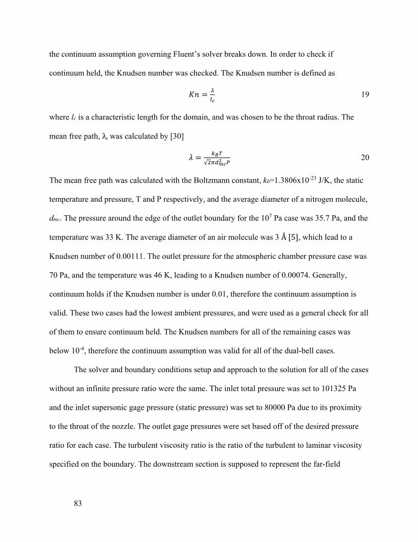
the continuum assumption governing Fluent’s solver breaks down. In order to check if
continuum held, the Knudsen number was checked. The Knudsen number is defined as
= 19
where lc is a characteristic length for the domain, and was chosen to be the throat radius. The
mean free path, , was calculated by [30]
= 20
The mean free path was calculated with the Boltzmann constant, kb=1.3806x10⁻²³ J/K, the static
temperature and pressure, T and P respectively, and the average diameter of a nitrogen molecule,
dmc. The pressure around the edge of the outlet boundary for the 107 Pa case was 35.7 Pa, and the
temperature was 33 K. The average diameter of an air molecule was 3 Å [5], which lead to a
Knudsen number of 0.00111. The outlet pressure for the atmospheric chamber pressure case was
70 Pa, and the temperature was 46 K, leading to a Knudsen number of 0.00074. Generally,
continuum holds if the Knudsen number is under 0.01, therefore the continuum assumption is
valid. These two cases had the lowest ambient pressures, and were used as a general check for all
of them to ensure continuum held. The Knudsen numbers for all of the remaining cases was
below 10-4, therefore the continuum assumption was valid for all of the dual-bell cases.
The solver and boundary conditions setup and approach to the solution for all of the cases
without an infinite pressure ratio were the same. The inlet total pressure was set to 101325 Pa
and the inlet supersonic gage pressure (static pressure) was set to 80000 Pa due to its proximity
to the throat of the nozzle. The outlet gage pressures were set based off of the desired pressure
ratio for each case. The turbulent viscosity ratio is the ratio of the turbulent to laminar viscosity
specified on the boundary. The downstream section is supposed to represent the far-field
83

conditions, therefore the ratio was changed to 1 instead of kept at 10. The reference location was
the inlet with all of the unchanged until after the solution converged.
Each case initiated iterations using a Courant number of 0.1 and a first-order upwind
scheme until the solution converged. Then, without reinitializing the solution, the scheme was
changed to second-order upwind, leaving the Courant number the same, and the calculation was
continued. If the residuals remained almost constant for over 15000 iterations, the courant
number was increased. Increasing the courant number increased the time step, and would not
negatively affect the solution because the finite volume scheme that Fluent uses is implicit [22].
Allowing the first-order solution to converge provided the solver with a better initial guess of the
solution than just using the original inlet and outlet boundary conditions, and helped prevent
deterioration of the solution along the outermost edges of the downstream boundary in all but
one case.
Figure 46: Dual-bell Mach contours for design point pressure ratios of 150 (top) and 1000 (bottom)
84

The design points for the dual-bell nozzle, where perfectly expanded flow is expected for
each, were both over-expanded. The top Mach contour in Figure 46 shows the dual-bell nozzle
Mach contour with a pressure ratio of 150 and the bottom shows the Mach contour for the
pressure ratio of 1000. Apart from the free stream separation, FSS, formation stemming from the
throat, another very mild flow feature appears to come off the wall from the beginning of the
second bell. FSS is the flow phenomena in parabolic nozzles where a shock stems from the
throat and exits the nozzle without reattaching to the nozzle wall. The waves cross one another
downstream of the nozzle and meet the right side of the boundary. Both cases have expansion
waves at the exit of the nozzle, meaning they are under-expanded. The first case should be over-
expanded in the first bell with a pressure ratio of 150, and perfectly expanded in the second bell
with a pressure ratio of 1000. The over-expansion in both cases could be caused by boundary
layers preventing full expansion of the flow until after it reaches the exit. A result of this is that
the average pressure over the nozzle exit plane would be higher than the expected 101.3 Pa. The
mass-averaged pressure over the nozzle’s exit for both cases is 1150 Pa. Furthermore, the full
plume from the nozzle is not seen in the downstream section, which suggests that future work
could involve modeling the same case with a larger downstream section.
Three over-expanded cases, shown in Figure 47, converged with pressure ratios between
4 and 50. The case with smallest pressure ratio that converged had an ambient pressure of 25000
Pa, which is equivalent to a pressure ratio of 4.05. All of the cases that converged had varied
levels of FSS starting just after the throat. The shocks never re-attach to the nozzle walls, which
is important in order to avoid shock heating and side loads. The over-expanded cases show how
oblique shocks regress into the nozzle becoming a normal shock at the exit plane and eventually
moving back towards the throat.
85

Figure 47: Dual-bell Mach contours for pressure ratios of 4.05, 10, and 20.26 in order from top to bottom
Figure 47 shows three over-expanded dual-bell nozzle Mach contours for pressure ratios
between 4.05 through 20.26. The largest Mach number among the three cases is 3.98, which is
reached with a pressure ratio of 20.26. The maximum Mach number for the critically over-
expanded case, the top of Figure 47, is about 3.5 and occurs for a pressure ratio of 4.05. The flow
remains supersonic at the throat and about three quarters of the way down the first bell before a
being slowed by a normal shock. The flow becomes subsonic after the shock and remains
subsonic throughout the flow up to the exit boundary. With this pressure ratio, a normal shock is
expected where the radius of the nozzle is equal to about 6.1 cm, or about 5.5 cm axially
downstream of the nozzle throat, well before the start of the second bell (Appendix E). The
86

shock is located a little further down the nozzle, most likely due to boundary layer effects
preventing full expansion until further downstream.
In contrast to the previous case, the middle image in Figure 47 shows the Mach contour
for a pressure ratio of 10, where a normal shock is located just beyond the exit plane of the
nozzle. Furthermore, the flow separates just before the end of the nozzle forming to small
oblique shocks that connect to the normal shock. The maximum Mach number for the pressure
ratio of 10 is 3.8, and is reached just upstream of the shock and where the oblique shocks from
the FSS meet along the centerline of the nozzle.
Two oblique shocks originating at the edge of the nozzle connect downstream of the exit
in the Mach contours for the 20.26 pressure ratio case in the bottom of Figure 47. The shocks
slightly over-compress the flow, causing a rebounding expansion fan leading to another oblique
shock after the initial connection, creating a Mach diamond. This is a realistic and expected
effect, and the maximum Mach number in the second diamond, about 2, is significantly less than
that coming out of the nozzle, about 4. If there were a larger downstream section, the Mach
diamonds would theoretically get weaker and weaker until they disappear.
87

Figure 48: Dual-bell Mach contours for pressure ratios of 50 (top) and 100 (bottom)
The top image in Figure 48 shows the case where the pressure ratio was set to 50.
Oblique shocks originate at the edge of the nozzle at a very slight angle from horizontal, barely
compressing the flow. The beginning of a Mach diamond formation appears to form after the
oblique shocks meet downstream of the nozzle. However, the downstream section ends before a
full diamond could form. The lower contour in Figure 48 was the case where the pressure ratio
was 100. This case is slightly under-expanded in the first bell, as can be seen from the flow
features starting at the inflection point.
5.3.3 2-D Simulation of Rao Wind Tunnel Contours
During Fluent evaluation of the wind tunnel contours, the Rao cases and the dual-bell
cases were tested in the same way. Each of these evaluations was two-dimension, but was not
axisymmetric; the flow was bounded on the top and bottom by walls. The convergence criteria
88

were kept as the Fluent standard: 1e-3 for all residual values. In addition, the same mesh for each
case was used throughout the testing. The only equations active were the energy equation and the
standard k-epsilon turbulence model. Included in the turbulence models is the no-slip condition
for walls. The fluid equation of state was the standard ideal-gas model for air included with
Fluent. The inlet pressure was set to 101325 Pa (1 atm), while the exit pressure was varied.
During testing, the Courant number was changed to accelerate convergence. Every case started
with a Courant number between 0.5 and 1.0, which was raised with each subsequent iteration
period. The standard iteration period was 15000 or 30000 iterations for the dual-bell and Rao
cases respectively. All other factors were held constant throughout testing.
There were certain cases that would not converge in a reasonable amount of time or
returned anomalous results. For these cases, a slightly different procedure was followed. First,
the test was run with first-order solutions to get a general idea of the flow pattern. Once that
solution was achieved, the flow equations were changed to second-order solutions to get a more
detailed image of the flow. This saved a considerable amount of computational time and lead to
more accurate results.
For the Rao nozzle testing, a variety of back pressures were chosen to create a time-lapse
series of snapshots of the flow field through the contours. As the flow passes through the wind
tunnel, the back pressure rises, which changes the pressure ratio. After consideration of critical
points (e.g. the design back pressure, the design pressure for the inflection point, the back
pressure for unchoked flow), a pseudo-logarithmic scale was chosen for the back pressures over
the range of back pressures present during testing. These values are listed in
Table 10 below.
89

Table 10: Summary of Convergence and Mass Flow Error for Rao Wind Tunnel Contour Cases
Back Pressure (Pa) Number of Iterations to Convergence Percentage Error in Mass Flow Rate
6.6 13440 0.381%
100 13420 0.452%
1000 13640 0.462%
5000 16600 1.901%
10,000 59120 1.420%
25,000 31360 0.049%
50,000 28440 5.225%
75,000 31340 0.874%
Figure 49: Comparison of Mach Contours at Varying Back Pressures in Rao Nozzle Wind Tunnel Contour
90
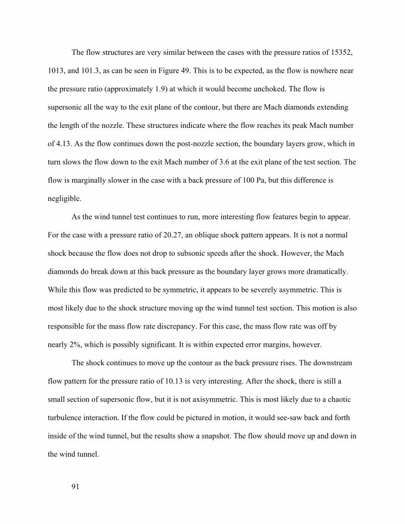
The flow structures are very similar between the cases with the pressure ratios of 15352,
1013, and 101.3, as can be seen in Figure 49. This is to be expected, as the flow is nowhere near
the pressure ratio (approximately 1.9) at which it would become unchoked. The flow is
supersonic all the way to the exit plane of the contour, but there are Mach diamonds extending
the length of the nozzle. These structures indicate where the flow reaches its peak Mach number
of 4.13. As the flow continues down the post-nozzle section, the boundary layers grow, which in
turn slows the flow down to the exit Mach number of 3.6 at the exit plane of the test section. The
flow is marginally slower in the case with a back pressure of 100 Pa, but this difference is
negligible.
As the wind tunnel test continues to run, more interesting flow features begin to appear.
For the case with a pressure ratio of 20.27, an oblique shock pattern appears. It is not a normal
shock because the flow does not drop to subsonic speeds after the shock. However, the Mach
diamonds do break down at this back pressure as the boundary layer grows more dramatically.
While this flow was predicted to be symmetric, it appears to be severely asymmetric. This is
most likely due to the shock structure moving up the wind tunnel test section. This motion is also
responsible for the mass flow rate discrepancy. For this case, the mass flow rate was off by
nearly 2%, which is possibly significant. It is within expected error margins, however.
The shock continues to move up the contour as the back pressure rises. The downstream
flow pattern for the pressure ratio of 10.13 is very interesting. After the shock, there is still a
small section of supersonic flow, but it is not axisymmetric. This is most likely due to a chaotic
turbulence interaction. If the flow could be pictured in motion, it would see-saw back and forth
inside of the wind tunnel, but the results show a snapshot. The flow should move up and down in
the wind tunnel.
91

Once the pressure ratio drops to 4.053, the shock has disappeared. The pressure gradient
does not allow for a shock beyond this point. However, a small region in the flow becomes
supersonic just downstream of the throat. This region ends a quarter of the length downstream of
the nozzle. The flow is grossly under-expanded for the final three cases. In fact, all three of these
cases are relatively similar. They all show a static image of a flow that should be bouncing back
and forth. However, this is contrary to the expectation of symmetric flow. This discrepancy is
one that could have a few different causes, including small geometry errors, chaotic turbulence
effects, or something within the solver of Fluent.
As the back pressure rises, the flow continues to slow down. The maximum Mach
number for a pressure ratio of 2.027 is only 1.8, and the flow is not supersonic all the way across
the throat. This is somewhat expected, as the critical pressure ratio for choked flow is 1.893, very
close to the pressure ratio for this case. In addition, the presence of boundary layers reduces the
effective nozzle throat area, increasing the velocity of the flow. The 1.351 case has effectively
the same results as the 2.027 case, but with a slower flow. However, the 1.351 case should be
unchoked flow. This is most likely due to a Fluent error.
5.3.4 2-D Simulation of Dual-Bell Wind Tunnel Contours
For the dual-bell nozzle, the same back pressures were used as in the Rao testing cases.
This was done to improve comparability between cases. One key note about the dual-bell nozzle
is the fact that the nozzle throat is approximately one-half the height of the Rao nozzle. This was
done to better simulate the pressure ratios present in the full-scale nozzle. As the exit height of
the wind tunnel is fixed, the only option was to reduce the height of the throat. Again, the goal of
the dual-bell testing was to create a rough, time-lapse picture of the flow structure as a function
of back pressure. Some comparison details between the cases are detailed in Table 11 below.
92

Table 11: Summary of Dual-Bell Contour Testing
Back Pressure (Pa) Number of Iterations to Convergence Percentage Error in Mass Flow Rate
6.6 129600 0.079%
100 19980 0.349%
1000 26640 0.315%
5000 44580 2.231%
10,000 108020 0.079%
25,000 44260 0.576%
50,000 154420 0.093%
75,000 154860 0.068%
Figure 50: Comparison of Mach Contours for the Dual-bell Contours
93

The flow structures for the first three back pressures are again very similar. Again, there
is a Mach diamond structure that starts just beyond the exit of the nozzle. However, the
maximum Mach number is 5.1 for each of these cases. This is to be expected for this case, as the
throat area was reduced, resulting in a larger expansion ratio. One interesting feature of these
flows is the very small subsonic region about two nozzle lengths downstream of the end of the
nozzle. This feature truncates the Mach diamonds. The reason for this structure is unclear, but it
could be an artifact of the dual-bell contour as it does not appear in the Rao testing cases. For
these pressure ratios, the second bell will be in use; that is, the flow will fully expand into the
second bell of the nozzle.
The flow structure in the nozzle begins to break down once the pressure ratio reaches 20.
In this flow, there are bubbles of supersonic flow in a narrow jet. This jet is axisymmetric, but
due to friction effects, the actual flow is shifted downward. The flow is completely full in the
first bell nozzle, but then the flow separates in the second bell.
This flow “breakdown” continues, albeit in a slightly different pattern, as the pressure
ratio continues to fall. When the pressure ratio reaches 10, the flow has become over-expanded.
At this point, the flow should be free to see-saw in the wind tunnel. As before, the fact that these
are snapshots, limit how effectively the images capture what is going on as the pressure changes.
One interesting point is the fact that the Mach number remains relatively high at this pressure
ratio. The maximum Mach number is approximately 3.8, or almost as fast as the unrestricted
flow in the Rao contours. Within the over-expanded flow, there are small Mach diamond-esque
structures.
However, when the pressure ratio falls to 4, the Mach pattern breaks down and
disappears. In addition, the Mach number falls to less than 2. The flow is even more grossly
94

over-expanded for this case. The final two test cases are fairly similar to the previous test case.
Both flows are non-symmetric and effectively subsonic. The maximum Mach number for the
75000 case is only 1.2 and is only reached in a localized region of the throat. The flows are
unchoked; however, the mass flow rates are the same as the choked flow rates. This discrepancy
was noted and do impact the results. However, the flow should be very close to choked, lending
veracity to the idea that the mass flow rate is off by a small amount.
95
6 Analysis and Discussion
The flow structures imaged in tests using the dual-bell contours are consistent with those
obtained through Fluent analysis of the dual-bell wind tunnel contour. Using the CFD-Post
subsection of ANSYS Workbench 14.5, a plot of the density gradients was created. As this is
what we see in schlieren imaging, these results are directly comparable as qualitative data.
6.1 Comparison of CFD and Schlieren Results
6.1.1 Rao Nozzle Results
During the initial stages of the test, both images (CFD-generated pressure gradient and
schlieren) are very similar, with very small density gradients. This is to be expected as this flow
is laminar and undisturbed. As the test progresses, a shock wave moves upstream in the test
section, immediately followed by a turbulent flow. This can be seen in Figure 51 and Figure 29.
As the test continued, the shock wave progressed upstream in the test section into the nozzle.
This can be seen between Figure 51 and Figure 52 (where Figure 52 is chronologically first).
Due to the limits of the Fluent testing (the Fluent simulations were not performed at every back
pressure), this flow feature was lost in the “time” gap between tests. To create Figure 51, surface
plots were created using CFD-Post, an adjunct to the ANSYS Workbench software. Each image
had 200 contour levels. The colormap used is the standard inverse grayscale scheme. The range
of values for the density gradient were automatically determined by CFD-Post and were left as
the full range present in the entire wind tunnel structure, from inlet to outlet flange.
96

Figure 51: Fluent "schlieren" image at a pressure ratio of 4.
Figure 52: Shock wave imaged using Fluent "schlieren" settings at a BP of 10.
Once the shock wave reached the throat of the nozzle, downstream effects became readily
apparent. One interesting feature of this shock is the shape. While it is an oblique shock, there is
a small section of the shock that is perpendicular to the test section walls. However, the Fluent
results show that the oblique shocks angle upstream from the perpendicular section, while the
physical testing indicates that the oblique shocks angle downstream. This is possibly due to a
flaw in the boundary conditions of the Fluent model at the walls of the test section.
Downstream of the shock, both flows have asymmetric flow features. In the wind tunnel
testing, these take the form of bright circular spots, as highlighted in Figure 31. These flow
features continue to form after the shock disappears from the schlieren image. The first spot
97

remains relatively steady, but subsequent spots follow a “line” up to immediately behind the
first, whereupon they also remain steady. This feature was captured in a preliminary form in the
Fluent plots. In Figure 53, there is a bright patch immediately downstream of a shock wave. This
appears to be the genesis of the bright circular spots.
Figure 53: Genesis of the flow features in the Rao test section.
6.1.2 Dual-Bell Results
The most distinctive result from the dual-bell testing was the imaging of the boundary
layer flow features, as seen in Figure 54. These features acted almost identically to the flow
features present in the Rao nozzle; that is, each subsequent feature started near the exit of the
nozzle and moved upstream to immediately behind the next feature upstream.
Figure 54: Fluent "schlieren" imaging at a pressure ratio of 10.
98

The bright spots were not as clearly imaged in the Fluent testing. In Figure 55, a distinct
region of high density gradient is clearly seen along the path of the flow features. However, it is
mirrored vertically. With that said, the jet does switch from top to bottom over the course of the
Fluent test cases. This is potentially due to a boundary layer effect that was not accounted for in
the simulation equations. This “switching” behavior was not seen in the physical experimental
results.
Figure 55: Fluent "schlieren" image at a pressure ratio of 4.
However, in the broader picture, the flows are very similar. Compare Figure 56 and
Figure 34. The primary feature to notice is the sloping dark line sweeping from just downstream
of the throat to the inflection point. This shock is also present in the Fluent results. At the next
pressure ratio for the Fluent test, the shock had disappeared (see Figure 55), which was also the
behavior observed in the experiments.
99

Figure 56: Fluent "schlieren” image at a pressure ratio of 10.
6.2 Full-Scale Nozzle Performance Comparison
In a qualitative comparison, the full-scale conventional nozzle analyzed with Fluent
performed similarly to the dual-bell nozzle in terms of the downstream behavior. The design
pressure ratio of the conventional contour was 102, and like the dual-bell nozzle, it showed over-
expanded behavior at the design pressure ratio, even though perfectly expanded behavior was
expected based on isentropic flow relations. The main difference between the two contours can
be seen in the internal flow structures. The flow within the conventional contour differed from
the dual-bell nozzle in that in there was only boundary layer separation within the nozzle. No
secondary flow structures formed, and the core flow was smooth as it reached the exit for the
design point case. The only extra core structures within the flow occurred in the under-expanded
case where an oblique shock from the nozzle’s edge met the core flow causing minor
disturbances downstream that carried through into the Mach discs.
The average specific impulse, for these cold flow cases, was calculated over a range of
back pressures using the mass averaged pressure and velocity from Fluent post-processing over
the nozzle’s exit plane. The mass averaged values were used instead of area-averaged values
because the difference was negligible. Fluent computed the mass averaged pressure and velocity
100

over the nozzle outlet for both the dual-bell and Rao nozzles. These values were input into the
rocket thrust equation to calculate the theoretical thrust produced by each nozzle and the specific
impulse was calculated using the thrust and mass flow rate. The thrust, T, which the nozzle
produced was calculated using the ideal thrust equation.
= + ( ) 21
where is the mass flow rate, ue is the exit velocity, Ae is the exit area and pe and pa are the exit
pressure and ambient pressure respectively. The specific impulse, , was calculated by dividing
the thrust by the mass flow rate, , and Earth’s gravitational constant, g0, for each case and then
averaging over the four cases. These calculations assumed a range of pressure ratios from 1.4 to
approximately 15000, with a chamber pressure of 1 atm. The temperature was 300K and air
(molar mass of 28 kg/kmol) modeled as an ideal gas was the working fluid.
= 22
Table 12 and Table 13 summarize the parameters for the dual-bell and Rao nozzles.
Table 12: Dual-bell nozzle specific impulse calculation parameters
PR Pe (avg)
(Pa)
Ve (avg)
(m/s) Thrust (N) Isp
1000 1147 655 499 70.233
150 1147 656 492.3 69.293
100 1147 656 484.4 68.183
50 1150 655 449.8 63.302
20 1177 653 385.2 53.479
10 3316 587 258.5 36.377
4 24448 216 142 20.124
101

Table 13: Rao nozzle specific impulse calculation parameters
PR Pe (avg)
(Pa)
Ve (avg)
(m/s) Thrust (N) Isp
15352 4472 593 594.947 85.868
1013 4472 593 594.947 85.868
10 4517 592 298.159 43.033
4 4902 586 -435.784 62.896
2 4839 587 -358.215 51.700
1.4 61632 228 155.661 22.466
The negative thrust values are unrealistic results that were produced by Fluent. Both of
the cases with negative thrust values had a normal shock at the end of the nozzle. The algebraic
average specific impulse was 64.9 s for the dual-bell contour and 71.6 s for the conventional
contour nozzle. The averages were only taking into account the cases that did not have a normal
shock in or at the exit plane of the nozzle. The Isp values were comparing the simulated flow
features for each nozzle. The Rao nozzle was optimized for a considerably lower pressure ratio
than the dual-bell. The dual-bell contour did not perform as well as the conventional nozzle
contour. This could be due to the location of the inflection point on the dual-bell contour, to the
optimal pressure ratio for each inflection, to boundary layer growth, or a combination of all
three.
6.3 Physical Interpretation
The high contrast structures in both the schlieren images and Fluent wind-tunnel
simulations are consistent with expected shock structures in a high speed nozzle. The structures
are more developed farther along the flow field in the Fluent simulation than in the schlieren
images, likely due to non-orthogonality in the alignment of the optical system with the wind
102

tunnel test section. The round light regions that appear in the schlieren images and correspond to
a similar density gradient in the Fluent simulations are a boundary flow structure of some kind.
The dark streaks seen in the schlieren images could potentially represent oblique shocks, the
reflections and interference of which result in the small, constant-density regions, which were
manifested as the round light regions.
103

7 Conclusion and Recommendations for Future Work
7.1 Conclusion
This project addressed a common issue in nozzle design and its effect on the efficiency of
rocket engine systems. A dual-bell nozzle contour design procedure was developed and used to
investigate a possible nozzle that could be implemented on a sounding rocket or other form of a
nanosatellite launch vehicle. The contour was adapted for physical testing in a supersonic wind
tunnel in conjunction with a schlieren optical system. This system captured images of normal
and oblique shock structures and boundary layer flow features in both the Rao and dual-bell
nozzles.
Schlieren imaging of flow in the tunnel showed oblique shock structures and boundary
layer flow features. Analysis of the dual-bell contour in both configurations was performed using
ANSYS Fluent simulations, and similar simulations were run for a conventional contour. This
was done to compare flow structures within the proposed dual-bell contour to those of a
conventional nozzle contour as well as to compare their performance characteristics. The
conventional nozzle contour performed better than the proposed dual-bell contour over a range
of backpressures, with an average (cold flow) specific impulse of 71.6 s compared to the dual-
bell’s 64.9 s. Future investigations should focus on changing the location of the inflection point
within the nozzle as well as optimizing the design point pressure ratios. Mach contours generated
from the Fluent simulations show similar flow features to the schlieren images from the wind
tunnel testing indicating that the Fluent simulations are both valid and robust for this application.
104

7.2 Recommendations for Future Work
The geometry of the dual-bell contour in the wind tunnel produced supersonic speeds but
could have been improved through a more perfect sealing process. The O-rings were sealed
tightly using vacuum grease but there was a leak from the space in between the endplate and
bracket. The silicon used to seal these two pieces did not create a tight enough fit. This leak
meant that the vacuum chamber could not be pumped down as far, 17 milliTorr rather than 3
milliTorr, shortening the usable test time. A better sealing process or sealant could ensure a more
accurate flow for comparison with CFD results.
Figure 57: Wind Tunnel with Dual-Bell Contours Installed
This project focused on the presence of an inflection point and two area ratios, but not the
location or shape of the inflection. Future testing could compare performance as the inflection
Possible Leak?
Brackets End Plate
105

point is moved toward the back of the nozzle. Similarly, a study of the flow structures coming
off of differently shaped (sharper or smoother) inflection points could improve performance.
In addition to schlieren images, pressure and velocity data could be gathered. Adding
pressure taps with Pitot probes on one side of the contour would allow for pressure
measurements along the test section.
This group calculated the wind tunnel run time based on varying throat diameters, but a
full back pressure versus run time calculation would facilitate comparison with the CFD results.
Knowing the backpressure vs. time (for example by collecting chamber pressure data during a
run), schlieren images and numerical data could be precisely aligned, enabling more accurate
comparison with Fluent results.
This group performed Fluent simulations using a steady-state (stationary solution)
approximation simplifying each case by assuming it corresponded to a single pressure ratio. The
next step to improve the simulation accuracy is to run transient cases covering the whole range of
expected pressure ratios. These simulations would require a pressure trajectory profile for the
rocket’s flight. A code detailing backpressure vs. altitude data needs to be added to Fluent
through a journal file in order to create a user defined function. This would then be implemented
to perform the transient calculation.
A time dependent simulation would enable a better performance comparison between
dual-bell and Rao contours throughout every pressure ratio, and a trajectory averaged specific
impulse value could be calculated. This case comparison (transient dual-bell compared to
transient Rao nozzle with trajectory information) would either validate or disprove whether or
not the dual-bell nozzle is effective.
106

A new Rao contour should be created that is optimized for a higher altitude (the current
nozzle is optimized for sea level operations) in order to obtain a more accurate comparison
between the dual-bell nozzle and the Rao nozzle performance.
107

8 References
[1] ÖSTLUND, J. 2002. Flow Processes in Rocket Engine Nozzles with Focus on Flow Separation and Side-Loads. Royal Institute of Technology.
[2] HAGEMANN, G., IMMICH, H., NGUYEN, T. V. & DUMNOV, G. E. 1998. Advanced rocket nozzles. Journal of Propulsion and Power, 14,620-634.
[3] NÜRNBERGER-GENIN, C. & STARK, R. 2009. Flow transition in dual bell nozzles. Shock Waves, 19, 265-270.
[4] NASUTI, F., ONOFRI, M. & MARTELLI, E. 2005. Role of wall shape on the transition in axisymmetric dual-bell nozzles. Journal of propulsion and power, 21, 243-250.
[5] SUTTON, G. 2010. Rocket Propulsion Elements, Wiley.
[6] KULHANEK, S. 2012. Design, Analysis, and Simulation of Rocket Propulsion System. Master of Science, University of Kansas.
[7] VERMA, S. B., STARK, R. & HAIDN, O. 2012. Gas Density Effects on Dual-Bell Transition Behavior. Journal of Propulsion and Power,28, 9.
[8] HAGEMANN, G. & FREY, M. 2008. Shock pattern in the plume of rocket nozzles: Needs for design consideration Shock Waves, 9.
[9] HORN, M. & FISHER, S. Dual-bell altitude compensating nozzles. NASA Propulsion Engineering Research Center, 1993. 140-147.
[10] FREY, M. & HAGEMANN, G. 1999. Critical assessment of dual-bell nozzles. Journal of propulsion and power, 15, 137-143.
[11] JONES, J. E. 2013. Nanolaunch 1200. NASA-Marshall Space Flight Center.
[12] MOORE, T. 2006. Black Brandt Sounding Rocket Returns to Flight.CPIAC Bulletin [Online], 32.
[13] SETTLES, G. S. 2001. Schlieren and Shadowgraph Techniques: Visualizing Phenomena in Transparent Media. Heidelberg, Germany: Springer-Verlag Berlin Heidelberg.
[14] NÜRNBERGER-GÉNIN, C. & STARK, R. 2010. Experimental Study on Flow Transition in Dual-Bell Nozzles. Journal of Propulsion and Power,26, 6.
[15] STARK, R., BOHM, C., HAIDN, O. J. & ZIMMERMANN, H. 2006. Cold Flow Testing of Dual-Bell Nozzles in Altitude Simulation Chambers.European Conference for Aerospace Sciences. DLR, German Aerospace Center.
[16] AULD & SRINIVAS 2006. A Body Placed in Subsonic and Supersonic Flows. Aerodynamics for Students.
[17] NASA GLENN RESEARCH CENTER 2000. Boundary Layer.
[18] 2007. Families of Turbulence Models [Online]. Available: http://www.innovative-cfd.com/turbulence-model.html [Accessed 09/26/2013.
[19] RUMSEY, C. Turbulence Modeling Resource [Online]. Available: http://turbmodels.larc.nasa.gov/ [Accessed 09/26/2013.
[20] GEORGESCU, A.-M., GEORGESCU, S.-Versus Fluent: 2D Numerical Simulation of the Stationary Flow Around a Blade of the Achard Turbine. 3rd Workshop on Vortex Dominated Flows 52(66), 10.
[21] AKIN, J. E. 1994. Finite Elements for Analysis and Design, San Diego, CA, Academic Press Limited.
[22] Fluent 2005. Introductory Fluent Notes. In: CENTER, F. U. S. (ed.).
108

[23] MOIN, P. & MAHESH, K. 1998. Direct Numerical Simulation: A Tool in Turbulence Research. Annual Review of Fluid Mechanics, 40.
[24] MATHEW, J. 2010. Large Eddy Simulation. Defence Science Journal, 60,8.
[25] SPALART, P. R. 2009. Detached-Eddy Simulation. Annual Review of Fluid Mechanics, 24.
[26] DURBIN, P. P.-R., B. A. 2010. Statistical Theory and Modeling for Turbulent Flow. 2nd ed. Hoboken, NJ, USA: Wiley
[27] BUGDEN, W., FITTON, K., FOLINAS, G., FOURNIER, N., HOGAN, G., ITO, M., LAMBERT, J., PATEL, N., SHIN, D.-U., WONG, G. & ZIEGLER, E. 2013. Design and Construction of a Supersonic Wind Tunnel with Diagnostics Worcester, Massachusetts: Worcester Polytechnic Institute.
[28] COMSOL. 2013. Multiphysics Simulation Software [Online]. [Accessed September 30, 2013].
[29] NESMEN, T. (2001). Fluctuating Pressure Data from 2-D Nozzle Cold Flow Tests (Dual Bell). Paper presented at the STD Fluids Workshop 2001, Marshall Space Flight Center
[30] KRUGER, & VINCENTI. (1965). Introduction to Physical Gas Dynamics. New York, New York: Wiley & Sons INC
109

Appendix A: AIAA Paper
Experimental and Computational Investigation of a Dual-Bell Nozzle
Kate Davis1, Elizabeth Fortner2, Michael Heard3, Hannah McCallum4, and Hunter Putzke5 Worcester Polytechnic Institute, Worcester, Massachusetts, 01609, USA
The proliferation of earth orbital missions enabled by nanosatellites, of which CubeSats are the most common, has focused increased attention on low-cost, mobile launch systems. Advanced nozzle design can address the demand for higher booster performance, and has resulted in the investigation of alternate nozzle geometry. A dual-bell nozzle represents a novel approach to this problem by utilizing two theoretically ideal design points over the ascent trajectory instead of just one. The primary focus for this project was to investigate the performance of a representative dual-bell nozzle both computationally and experimentally. First, a dual-bell nozzle was designed which could be used on a representative, nanosatellite launch system with design altitudes of 3 km and 17 km. The nozzle contours were modified to facilitate machining, and incorporated in a supersonic wind tunnel. The dual-bell nozzle fabricated for testing in the wind tunnel had a “first contour” expansion ratio of 1:9.85 corresponding to an ideal design pressure ratio of 134. The downstream, “second contour” had an expansion ratio of 1:19.7 corresponding to an ideal design pressure ratio of 374. The conventional nozzle fabricated for testing in the wind tunnel had an expansion ratio of 1:11.3 corresponding to an ideal design pressure ratio of 102. Imaging of flow structures was achieved using a schlieren optical system. In addition, the computational fluid dynamics program ANSYS Fluent was used to model both a hypothetical, full-scale nozzle as well as the scaled version tested in the wind tunnel. Simulations were performed for full-scale, dual-bell nozzles operating at pressure ratios (chamber to ambient) of 20, 50, 100, 150 and 1000. These results were then compared to a similar conventional nozzle for each case. Preliminary schlieren results indicate that the scale wind tunnel dual-bell contours show flow structures consistent with the Fluent results.
Nomenclature
a,b,c = Coefficients of the parabola defining the nozzles A = Nozzle exit area g0 = Earth’s gravitational constant; 9.8 m/s2 Isp = Specific impulse K = Percentage of the length of an equivalent 15% conical nozzle
= Nozzle length = Mass flow rate
pa = Ambient pressure pe = Average pressure over the nozzle exit-plane R = Exit radius
= Nozzle radius at the inflection point = Radius of the nozzle at the connection between the throat and the first parabola
1 Undergraduate student, Mechanical Engineering Department, Aerospace Program, AIAA Student Member 2 Undergraduate student, Mechanical Engineering Department, Aerospace Program, AIAA Student Member 3 Undergraduate student, Mechanical Engineering Department, Aerospace Program, AIAA Student Member 4 Undergraduate student, Mechanical Engineering Department, Aerospace Program, AIAA Student Member 5 Undergraduate student, Mechanical Engineering Department, Aerospace Program, AIAA Student Member
110

= Nozzle radius at the throat = Thrust
= Axial position of inflection point = Axial position of the connection between the throat and the first parabola
= Nozzle area ratio = Nozzle exit angle = Flow angle at the connection between the throat and the first parabola
I. Introduction
goal of the aerospace engineering community is to develop more efficient and reliable methods to transport payloads into orbit. The increasing prevalence of nanosatellites and lack of small payload (<10 kg) launch vehicles combined with the demand for higher rocket performance has led to the critical assessment of rocket
engine subsystems. Numerous studies have focused on the exhaust nozzle with the goal of creating the most efficient single-stage-to-orbit (SSTO) launch vehicle possible. This investigation focused on designing and comparing the differences between a dual-bell nozzle and a conventional nozzle computationally and experimentally. A dual-bell nozzle utilizes two theoretically ideal design points over the ascent trajectory instead of one by combining two parabolic contours separated by an inflection. The upstream contour corresponds to the lower altitude design point. Conventional nozzles refer to any nozzle with a single, continuous contour between the throat and the exit, and are optimally expanded at only one altitude. The dual-bell concept was first introduced in literature in 1949 by F. Cowles and C. Foster, and was patented in the 1960s by Rocketdyne1. Research activity was revived in the 1990s, in part due to the development of modern CFD capabilities. Tests at Rocketdyne conducted by Horn and Fisher and in Europe by the Future European Space Transportation Investigations Programme (FESTIP) at the European Space Agency (ESA) confirmed the feasibility of this nozzle design1. However, they also demonstrated that real dual-bell nozzles fall short of the theoretical optimum due to losses sustained from aspiration drag, earlier-than-ideal flow separation, and a non-optimal contour for high altitude flight. Even with these additional losses, Horn and Fisher found that a dual-bell nozzle could provide enough thrust to carry 12.1% more payload than a conventional nozzle of the same area ratio1. A dual-bell nozzle has three characteristic geometric features: an inner base nozzle contour, a wall inflection, and an outer extension nozzle contour. At low altitudes, exhaust gases expand in the base nozzle and separate at the inflection point, making the area at the inflection point the effective exit area during this mode of operation. By having controlled, axisymmetric flow separation, side loads are less of an issue than in conventional nozzles because the separation point cannot fluctuate when the nozzle is under-expanded. As the rocket altitude increases, ambient pressure decreases and the exhaust gases need a larger expansion ratio to match, or approach, the ambient conditions. During this operational phase, the flow is attached to the wall of the extension nozzle, and the whole exit area of the nozzle is used. Because of this second section of the nozzle, the flow is not as under-expanded as it would be for a conventional nozzle with the same area ratio as the base nozzle contour. Thus, the dual-bell nozzle achieves improved high altitude performance over single-bell nozzles2. Additionally, dual-bell nozzles have the unique benefit among altitude compensating nozzles of having no moving parts. Schlieren imaging, named after the German word for “streak,” is an optical technique for studying inhomogeneous media. August Toepler was the first to see the motion of shock waves using his schlieren technique. Since then, schlieren techniques have been further developed for various applications3. Schlieren systems are considered the standard for high-speed wind tunnel flow imaging, making it a perfect optical technique for this project. Information about the location and shape of shock waves, the location of boundary-layer separation, and areas of wave interference can be seen qualitatively using a schlieren system. The primary focus for this project was testing a dual-bell contour in an indraft supersonic wind tunnel and testing a hypothetical full-scale nozzle using ANSYS Fluent©. These results were then compared to a conventional nozzle for each case. In addition, Fluent was used to simulate the flow through the supersonic wind tunnel in order to assess the comparability of Fluent results and wind tunnel results. The flow seen in the wind tunnel was found to resemble the flow predicted by Fluent, which confirmed the possibility for an improved specific impulse and thereby an improved payload fraction.
II. Nozzle Design Methodology The area ratio of both the full-sized conventional nozzle and dual-bell nozzle was determined using the isentropic
flow relations. To size the throat of the nozzle, a thrust for the Black Brandt sounding rocket (the intended launch vehicle) was calculated. A chamber pressure of 1500 psi, given by the characteristics of the Black Brandt sounding rocket, a possible first stage for a CubeSat launch vehicle3, was used to determine the pressure ratios (stagnation to
A
111

ambient) at different altitudes. The pressure ratios were then back-solved to find Mach numbers and area ratios. The value of the ratio of specific heats was assumed to be 1.23 due to the large assumed pressure and the high temperatures expected inside the combustion chamber of the Black Brandt sounding rocket (a potential application for the dual-bell nozzle)4. The conventional nozzle was designed with an initial pressure ratio of 102 with a corresponding area ratio of 11.3 corresponding to an optimized altitude at sea level. The conventional nozzle was ideally expanded at sea level in order to have a full-sized, ideal testing case for a cold flow test. In comparison, the dual-bell nozzle design altitudes were calculated from the launch profile in order to have the most realistic possible results. The dual-bell nozzle’s area ratio at the inflection point is 15, and the area ratio at the exit is 64.5. The corresponding pressure ratios are 148 and 1000 for the inflection point and exit respectively. The design altitudes for the dual-bell nozzle are 3.05 km and 16.97 km.
A. Contour Design
The conventional nozzle is defined by three curves, the length of the nozzle, and the throat radius (Figure 1). The length of the nozzle is determined by
= 1
tan( ) (1)
where K is a percentage of the length of a 15° half e) conical nozzle with the same area ratio, Rt is
the throat radius, (found to be 0.0305 m)3 area ratio. In order to define the nozzle further, a coordinate system is defined with the axial (x) axis passing through the line of symmetry and the radial (y) axis centered at the throat. The first and second curves define the entrance and exit of the throat of the nozzle, and are based on circular curves. The third curve is a parabola and takes the form
= + + (2)
The coefficients a, b, and c, are determined by the derivatives of the contour at the point where the circle from the throat meets the beginning of the parabola, , and the length of the nozzle, . To close the system of equations and solve for the parabolic coefficients, the exit of the nozzle is examined, where x is equal to the nozzle’s length,
. In matrix form, the system is
2 1 0R 1
1= ( )
(3)
which can then be solved for the parabolic coefficients. The dual-bell contour adds a second parabola that connects two conventional contours that share the same throat
but are optimized for different altitudes (Figure 2). The second parabola defines the second bell section and connects the two contours thereby achieving a greater expansion ratio. The system of equations to solve for the coefficients of the second curve is:
Figure 1: Conventional parabolic nozzle [© Kulhanek, 20127]
Figure 2: Dual-Bell nozzle with labeled sections (axes scaled for clarity)
112

2 1 02 1 0
1=
1tan ( )
1tan ( )
(4)
where a’, b’ and c’ are the coefficients of the second curve. The final design parameters are listed in Table 1. Table 1: Design parameters for the full sized conventional and dual-bell nozzle
Type of Nozzle Conventional Nozzle Dual-Bell Nozzle (First Contour)
Dual-Bell Nozzle (Second Contour)
a 26.0287 10.2859 21.8315 b -0.5375 0.5084 -4.7223 c -0.0034 -0.0208 0.5362
Throat Radius (m) 0.0305 0.0305 Shared Length (m) 0.2150 0.3673 0.2732
Theta_N (degrees) 40.0000 40.0000 20.0000 Theta_e (degrees) 11.9409 14.237 9.5880
Area Ratio 11.2983 31.4754 64.5603 B. Supersonic Wind Tunnel Test Section Design
The nozzle contours, designed for the first stage of a nanosatellite launch vehicle, had to be scaled down to fit the wind tunnel test section. The size of the contours for the Fluent analysis and application are on the order of 0.5 – 1.0 meter in scale, while that of the test section is on the order of inches. In addition to the required dimensional scaling, the contour was also modified to adapt to the 2-D rectangular geometry inherent
to the test section. Modifying the code developed for the full-size nozzle completed preliminary design. Due to the constraints of the wind tunnel, the exit height of the wind tunnel was fixed to a maximum span of 26 mm. The area ratios of the machined nozzles were modified to be 9.85 and 19.7 for the inflection point and exit of the dual-bell nozzle and 11.3 for the conventional contour. The area ratios of the dual-bell nozzle were changed from their full-scale counterparts in order to keep the throat sizes within machine tolerances. The modified contours were then machined from aluminum blanks.
III. Wind Tunnel Testing
An indraft wind tunnel test setup was devised to test the nozzle contours that were
Figure 4: Wind tunnel dual-bell test section
Figure 3: CAD design of the wind tunnel (all dimensions are given in millimeters
98.5
25.8 1.29 33.1
305
113

simulated with Fluent. The wind tunnel consists of a ball valve, a test section into which contours can be inserted for testing, and a mounting flange that connects the whole system to a vacuum chamber. The valve and flange sections were reused from a previous project group7, but the parts in the test section, including the contours, either had to be modified or machined specifically for this project. Two sets of contours were machined: one set with dual-bell geometry, and another set with conventional geometry.
Flow structures in the wind tunnel were visualized using a schlieren-imaging system. Schlieren imaging works on the principle of refraction; parallel rays of light traveling through a homogenous density medium will continue to be parallel, but if parallel rays of light pass through a region where the density of the medium changes, then some of the rays of light will be refracted. In a schlieren imaging system, a series of lenses and mirrors direct parallel rays of light through a test section in which a flow phenomenon occurs. A razor blade cuts off half of the refracted rays of light, enabling a black and white image to be projected on a screen. These images form the qualitative data collected from the imaging system. Schlieren images show the density gradients in the air in the test section of the system: strong gradients appear as dark regions and weak gradients appear as light regions. In order to obtain the best images, the optical components must be precisely aligned.
A schlieren-imaging system was designed by a previous project group6, but the system required a redesign and optimization before it was functional. Using an x-channel base so that the components of the system could be easily repositioned, a series of optimization exercises were conducted to determine the best location for each component. The result of this optimization was a set of distances between components and angles between the three different segments of the system. In order to simplify the alignment of the optical components, the system was transferred from the x-channel to an optical plate with precision-drilled holes at the optimal locations of all the optical components.
Reliable operation of the vacuum chamber and precise alignment of the optical elements of the schlieren system was crucial to the success of the wind tunnel experiments. For each test, the optics of the schlieren system were realigned to negate any disturbance between tests. Once the optical elements were set, the vacuum chamber was pumped down to approximately 6.6 Pa and the test was started immediately after the pump was switched off. Starting the test at this point ensured that the pressure in the chamber did not have time to rise significantly (from any residual leaking), thus giving the largest initial pressure ratio and the longest test run time. During each test, a series of images were taken in quick succession throughout the entire duration, to capture any flow effects revealed by the schlieren system. These images were analyzed and compared to the results of the Fluent simulation, to determine how the results from the Fluent tests apply to real, physical flows.
Using the optimized schlieren system, images of flow structures were obtained during tests with the wind tunnel. Figure 5 contains images from two different tests of the wind tunnel operating with the dual-bell contour. The right side of the image is the upstream section, where a flow pattern is clearly visible on both tests. The bright flow areas formed on the end side of an oblique shock, which is visible in Figure 5(A).
IV. Fluent Analysis
The full-scale and the wind tunnel-scaled contours were analyzed using ANSYS Fluent, operating through Workbench 14.5™. The mesh for each case was generated using the Workbench mesh generator using quadrilateral cells. The full-scale models included a large downstream section in order to examine the flow structures downstream of the nozzle.
A hot-fire nozzle test for a solid rocket booster involves complex mixtures, including combusting reactants, un-combusted and partially combusted particles mixing with the flow, non-ideal gas behavior, and significant heat transfer effects. Due to the added complexity of a full hot fire test combined with the initial testing involving a supersonic wind tunnel, the Fluent simulations were constructed to model cold flow tests. This had the added benefit
Figure 5: Schlieren images for two different tests of the dual-bell nozzle contour
114
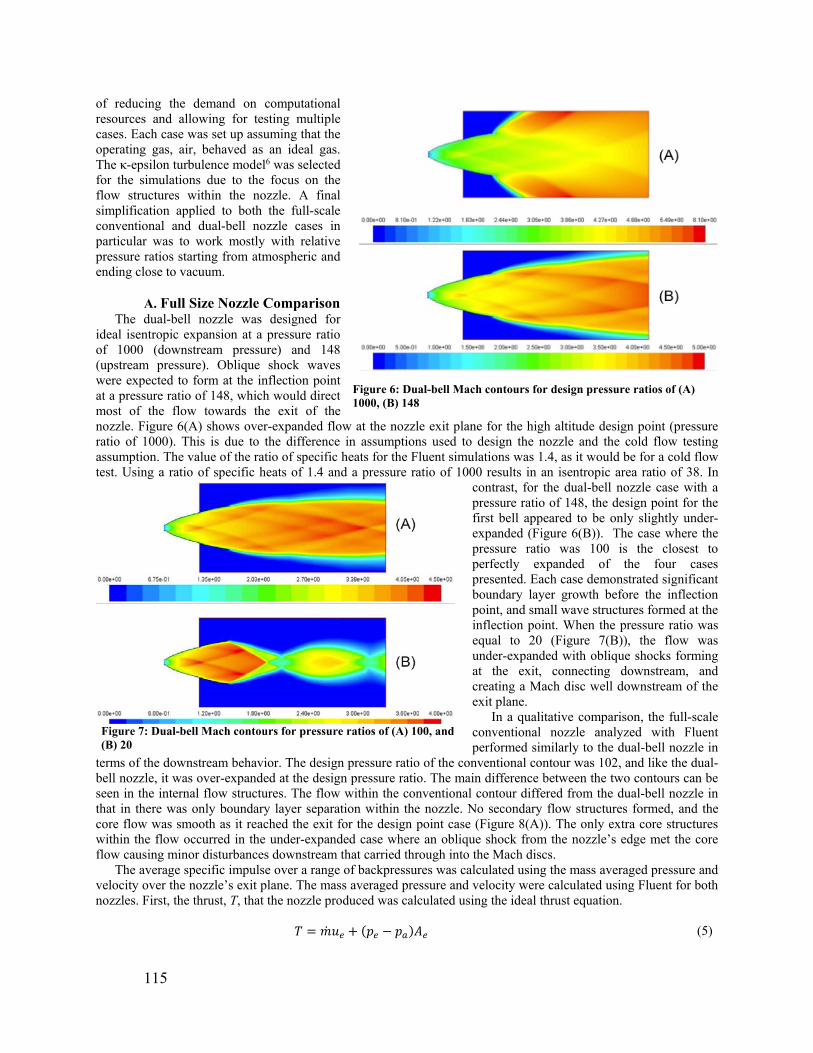
of reducing the demand on computational resources and allowing for testing multiple cases. Each case was set up assuming that the operating gas, air, behaved as an ideal gas.
-epsilon turbulence model6 was selected for the simulations due to the focus on the flow structures within the nozzle. A final simplification applied to both the full-scale conventional and dual-bell nozzle cases in particular was to work mostly with relative pressure ratios starting from atmospheric and ending close to vacuum.
A. Full Size Nozzle Comparison
The dual-bell nozzle was designed for ideal isentropic expansion at a pressure ratio of 1000 (downstream pressure) and 148 (upstream pressure). Oblique shock waves were expected to form at the inflection point at a pressure ratio of 148, which would direct most of the flow towards the exit of the nozzle. Figure 6(A) shows over-expanded flow at the nozzle exit plane for the high altitude design point (pressure ratio of 1000). This is due to the difference in assumptions used to design the nozzle and the cold flow testing assumption. The value of the ratio of specific heats for the Fluent simulations was 1.4, as it would be for a cold flow test. Using a ratio of specific heats of 1.4 and a pressure ratio of 1000 results in an isentropic area ratio of 38. In
contrast, for the dual-bell nozzle case with a pressure ratio of 148, the design point for the first bell appeared to be only slightly under-expanded (Figure 6(B)). The case where the pressure ratio was 100 is the closest to perfectly expanded of the four cases presented. Each case demonstrated significant boundary layer growth before the inflection point, and small wave structures formed at the inflection point. When the pressure ratio was equal to 20 (Figure 7(B)), the flow was under-expanded with oblique shocks forming at the exit, connecting downstream, and creating a Mach disc well downstream of the exit plane.
In a qualitative comparison, the full-scale conventional nozzle analyzed with Fluent performed similarly to the dual-bell nozzle in
terms of the downstream behavior. The design pressure ratio of the conventional contour was 102, and like the dual-bell nozzle, it was over-expanded at the design pressure ratio. The main difference between the two contours can be seen in the internal flow structures. The flow within the conventional contour differed from the dual-bell nozzle in that in there was only boundary layer separation within the nozzle. No secondary flow structures formed, and the core flow was smooth as it reached the exit for the design point case (Figure 8(A)). The only extra core structures within the flow occurred in the under-expanded case where an oblique shock from the nozzle’s edge met the core flow causing minor disturbances downstream that carried through into the Mach discs.
The average specific impulse over a range of backpressures was calculated using the mass averaged pressure and velocity over the nozzle’s exit plane. The mass averaged pressure and velocity were calculated using Fluent for both nozzles. First, the thrust, T, that the nozzle produced was calculated using the ideal thrust equation.
= + ( ) (5)
Figure 7: Dual-bell Mach contours for pressure ratios of (A) 100, and (B) 20
Figure 6: Dual-bell Mach contours for design pressure ratios of (A) 1000, (B) 148
115

Where is the mass flow rate, ue is the exit velocity, Ae is the exit area and pe and pa are the exit pressure and ambient pressure respectively. The specific impulse, , was calculated by dividing the thrust mass flow rate, , and Earth’s gravitational constant, g0, for each case and then averaging over the four cases.
= (6)
The algebraic average specific impulse was 64.9 s for the dual-bell contour and 71.6 s for the conventional contour nozzle. The dual-bell contour did not perform as well as the conventional nozzle contour. This could be due to the location of the inflection point on the dual-bell contour, to the optimal pressure ratio for each inflection, to boundary layer growth, or a combination of all three.
B. Wind Tunnel Conventional and Dual-Bell Contour Comparison
The flow through the indraft supersonic wind tunnel was simulated in ANSYS Fluent. Both scale model nozzle contours were tested in order to have a point of comparison between the computational and experimental testing. A variety of backpressures were chosen to create a time-lapse series of snapshots of the flow field through the contours. Each picture presented here is a surface plot of the Mach number throughout the simulation domain.
The first test case consisted of a test with a pressure ratio (inlet to outlet) of 1013. The inlet pressure was atmospheric, matching the physical wind tunnel. For the conventional nozzle (Figure 9(A)), the flow is supersonic all the way to the exit plane of the contour, and there are Mach diamonds extending the length of the test section.
The converging-diverging contour accelerates the flow to a peak Mach number of 4.13. As the flow continues down the post-nozzle section, a boundary layer grows, which slows the flow down to the exit Mach number of 3.6 at the center of the nozzle.
The second test case pressure ratio was 10, with the inlet pressure still remaining at atmospheric conditions. The flow is visible in Figure 9(B). There is a normal shock present just downstream of the exit of the nozzle. After the shock, a small section of the flow remains supersonic, but it is not symmetric. This is most likely due to a chaotic turbulence interaction and is a factor of over-expanded flow. If the flow could be pictured in motion, it would seesaw back and forth inside of the wind tunnel, but the results show a snapshot.
Figure 8: Conventional nozzle Mach contours for pressure ratios of (A) 1000 and (B) 10
Figure 9: Conventional nozzle wind tunnel Mach contours for pressure ratios of (A) 1000, (B) 10, and (C) 2
116

The final case would occur near the end of a test. The pressure ratio would be constantly falling, and therefore was set to 2, unchoking the nozzle as seen in Figure 9(C). In the computational results, there was still a small region of supersonic flow that was not predicted using 1D isentropic flow relations. However, the presence of a turbulent boundary layer may have created a smaller effective throat, pushing the pressure ratio threshold for choked flow down. In addition, the flow continued to exhibit the seesawing behavior seen in the previous case. All three tests were repeated for the dual-bell contour, as detailed in the next section.
The dual-bell test cases used a finer mesh than the conventional nozzle. This was a factor of the limits on the experimental testing and the different throat sizes. With the rougher mesh employed by the conventional nozzle, effects in and near the throat, as well as the effects due to the inflection point were masked and not clearly visible. In the interest of saving computational time, the meshes used were the simplest possible without losing a significant amount of clarity.
For the first test case, the dual-bell nozzle behaved in roughly the same way as the conventional nozzle, as is seen in Figure 10(A). Again, a Mach diamond structure started just beyond the exit of the nozzle. However, the maximum Mach number is 5.1 for this case due to the larger area ratio of the second bell. One interesting feature of these flows is the very small subsonic region about two nozzle lengths downstream of the end of the nozzle. This feature truncates the Mach diamonds. However, in the flow pattern itself, there are lines of reduced Mach number downstream of the inflection points. For this pressure ratio, both bells will be in full use. This would be equivalent to high-altitude flight for a launch vehicle.
In the second test case, major differences are seen when compared to the conventional nozzle. In the dual-bell test, the entire flow structure has broken down as is clearly visible in Figure 10(B). There is no clearly visible shock; instead, the flow has grossly over-expanded. This is expected, because the second bell of the contour is designed for a pressure ratio of 374 instead of the 102 for the conventional nozzle. The flow within the thin jet is still supersonic, reaching a Mach number of 3.5. There are small Mach diamond structures downstream of the core jet.
The third case for the dual-bell nozzle is similar to the conventional nozzle (Figure 10(C) and Figure 9(C), respectively). Again, there is a small supersonic region at the throat and the flow has tumbled off-center. The secondary flow jet is slightly smaller in the dual-bell case, as would be expected due to the smaller mass flow rate. The primary flow structure holds close to the upper contour at this instant, but we would expect the flow to not favor either direction.
V. Comparison of Schlieren Images and CFD Results
The flow structures imaged in tests using the dual-bell contours are consistent with those obtained through Fluent analysis of the dual-bell wind tunnel contour. Boundary layer flow features were observed on the schlieren images collected during wind tunnel testing of the dual-bell contour. These features were also noted in the Fluent simulations of the dual-bell wind-tunnel contours at a pressure ratio of 10 (Figure 10(B)). While these two images compare the density gradient of the flow and the Mach number, the Mach number is dependent on the density. The
Figure 11: Comparison of schlieren (top) and Fluent (bottom) images of the density gradient.
Figure 10: Dual-bell wind tunnel Mach contours for pressure ratios of (A) 1000, (B) 10, and (C) 2.
117

first boundary layer flow feature appeared approximately 18 seconds into a 115 second test. They were visible at the tail end of an oblique shock, which appeared approximately 15 seconds into the test. This phenomenon is shown in Figure 11, where a schlieren image (top) showing flow features noticed 18 sec into the test were captured by a density gradient plot generated by Fluent. This suggests that both sets of results were consistent with physical phenomena and are valid for this application.
VI. Conclusion
This project addressed a common issue in nozzle design and its effect on the efficiency of rocket engine systems. A dual-bell nozzle contour design procedure was developed and used to investigate a possible nozzle that could be implemented on a sounding rocket or nanosatellite launcher. The contour was adapted for physical testing in a supersonic wind tunnel. Schlieren imaging of flow in the tunnel showed oblique shock structures and boundary layer flow features. Analysis of the dual-bell contour in both configurations was performed using ANSYS Fluent simulations, and similar simulations were run for a conventional contour. This was done to compare flow structures within the proposed dual-bell contour to those of a conventional nozzle contour as well as to compare their performance characteristics. The conventional nozzle contour performed better than the proposed dual-bell contour, with an average specific impulse of 71.6 s compared to the dual-bell’s 64.9 s. Future investigations will examine changing the inflection point to different locations within the nozzle and optimizing the design point pressure ratios. Mach contours generated from the Fluent simulations show similar flow features to the schlieren images from the wind tunnel testing. This indicates that the Fluent simulations are both valid and robust for this application. Further research shall be conducted to measure flow characteristics in the wind tunnel for a more accurate comparison with the Fluent wind tunnel simulations, leading to development of a full-size nozzle for cold-flow testing.
Acknowledgments
We would like to thank Professor John Blandino for his help and guidance, Jonathon Jones of NASA for generously providing us with information on the ascent profile of the Nanolaunch 1250 launch system, and the WPI Machine Shop for their help in manufacturing the wind tunnel contours.
References
1Horn, M. & Fisher, S. Dual-bell altitude compensating nozzles. NASA Propulsion Engineering Research Center, 1993. 140-147. 2Hagemann, G., Immich, H., Nguyen, T. V. & Dumnov, G. E. 1998. Advanced rocket nozzles. Journal of Propulsion and Power, 14,620- 634. 3Jones, J. E. 2013. Nanolaunch 1200. NASA-Marshall Space Flight Center 4Ceviz, M, and Kaymaz, I. 2005. Temperature and air–fuel ratio dependent specific heat ratio functions for lean burned and unburned mixture. Journal of Energy Conversion Management, 46, 2387-2404. 5Settles, G. S. 2001. Schlieren and Shadowgraph Techniques: Visualizing Phenomena in Transparent Media. Heidelberg, Germany: Springer-Verlag Berlin Heidelberg. 6Moin, P. & Mahesh, K. 1998. Direct Numerical Simulation: A Tool in Turbulence Research. Annual Review of Fluid Mechanics, 40. 7Kulhanek, S. 2012. Design, Analysis, and Simulation of Rocket Propulsion System. Master of Science, University of Kansas. 8Bugden, W., Fitton, K., Folinas, G., Fournier, N., Hogan, G., Ito, M., Lambert, J., Patel, N., Shin, D.-U., Wong, G. & Ziegler, E. 2013. Design and Construction of a Supersonic Wind Tunnel with Diagnostics Worcester, Massachusetts: Worcester Polytechnic Institute. 9Östlund, J. 2002. Flow Processes in Rocket Engine Nozzles with Focus on Flow Separation and Side-Loads. Royal Institute of Technology. 10Nurnberger-Genin, C. & Stark, R. 2009. Flow transition in dual bell nozzles. Shock Waves, 19, 265-270. 11Nasuti, F., Onofri, M. & Martelli, E. 2005. Role of wall shape on the transition in axisymmetric dual-bell nozzles. Journal of propulsion and power, 21, 243-250. 12Sutton, G. 2010. Rocket Propulsion Elements, Wiley. 13Verma, S. B., Stark, R. & Haidn, O. 2012. Gas Density Effects on Dual-Bell Transition Behavior. Journal of Propulsion and Power,28, 9.
118

14Hagemann, G. & Frey, M. 2008. Shock pattern in the plume of rocket nozzles: Needs for design consideration Shock Waves, 9. 15Frey, M. & Hagemann, G. 1999. Critical assessment of dual-bell nozzles. Journal of propulsion and power, 15, 137-143. 16Nurnberger-Genin, C. & Stark, R. 2010. Experimental Study on Flow Transition in Dual-Bell Nozzles. Journal of Propulsion and Power,26, 6. 17Stark, R., Bohm, C., Haidn, O. J. & Zimmermann, H. 2006. Cold Flow Testing of Dual-Bell Nozzles in Altitude Simulation Chambers.European Conference for Aerospace Sciences. DLR, German Aerospace Center. 18Auld & Srinivas 2006. A Body Placed in Subsonic and Supersonic Flows. Aerodynamics for Students. 19Akin, J. E. 1994. Finite Elements for Analysis and Design, San Diego, CA, Academic Press Limited. 20Mathew, J. 2010. Large Eddy Simulation. Defence Science Journal, 60,8. 21Spalart, P. R. 2009. Detached-Eddy Simulation. Annual Review of Fluid Mechanics, 24. 22Durbin, P. P.-R., B. A. 2010. Statistical Theory and Modeling for Turbulent Flow. 2nd ed. Hoboken, NJ, USA: Wiley
119

Appendix B: How to Use the Schlieren System
1) Assemble the wind tunnel with the chosen contours, ensuring that caulk seals between the brackets and endplates are not broken and that the o-rings are in continuous contact with the windows.
2) Attach the wind tunnel to the vacuum chamber, ensuring that the windows are oriented perfectly vertically. Any error in the vertical orientation will result in light interference that will pollute the image.
3) Turn on the light. 4) Temporarily remove the slit and the razor blade from the light path and position the
schlieren system such that the silhouette of the desired area of the tunnel is shown on the screen. This involves moving the entire table. Be sure to keep the light path perpendicular to the wind tunnel.
5) Reposition the slit to focus the image on the screen (approximately 4 cm away from the collimating lens).
6) Reposition the razor blade to just beyond the focal point of the second mirror. Adjust the height of the blade so that it cuts off half of the light beam. The highest contrast images will be produced if the image is a uniform, dim shade while no test is being run.
7) Test the alignment by spraying compressed air or holding a candle near the test section.
Troubleshooting
If the image is out of focus, adjust the slit. If the image is low contrast, adjust the position and height of the razor blade. If the image has bright lines parallel to one of the contours, then the wind tunnel is not
perfectly vertical. Remove the schlieren system, loosen the bolts that connect the wind tunnel to the vacuum chamber, and adjust the position until it is vertical.
120

Figure 58: Example of Light Interference
121

Appendix C: Fluent Contours of Pressure
Rao Pressure Contours:
122

Dual-Bell Pressure Contours:
123

124

Rao Wind Tunnel Nozzle Pressure Contours
125
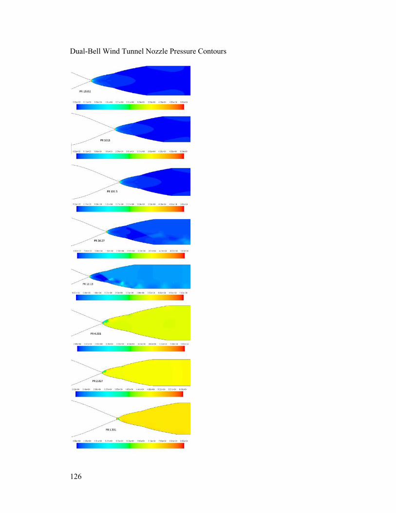
Dual-Bell Wind Tunnel Nozzle Pressure Contours
126

Appendix D: Parabolic Coefficient Calculations
First parabola length: = ( )
Equation of first curve: + ( ( + 1.5 )) = (1.5 )
Re-written: = (1.5 ) + 2.5
Equation of second curve: + ( ( + 0.382 )) = (0.382 )
Re-written: = (0.382 ) + 1.382
Derivative of first curve: = tan( ) =( . )
= 1.5 sin( )
Equation of parabola, for Rao and first parabola dual-bell:
= + +
Slope of parabola at point N: = tan( ) = ( . )
Slope of curve one at point N: = 0.382 sin ( )
Definition of xN: = + +
Slope at xN: = tan( ) =
Slope at exit (both dual-bell and Rao): = tan( ) =
Full system of equations for the parabolic coefficients for the first parabola (also includes the
only parabola for the Rao nozzle)
127

2 1 02 1 0
1=
1tan ( )
1tan ( )
Full length of dual-bell nozzle: = ( )
Full system of equations for the second parabola of the dual-bell nozzle:
2 1 02 1 0
1=
1tan ( )
1tan ( )
128

Note: The throat of the dual-bell nozzle is labeled and constructed the same as the Rao nozzle in
the pictures.
129

Appendix E: MATLAB Scripts
% Isentropic flow relations, pressure ratio input % Called by all of the following codes function [TR,PRt,TRt,M,AR]=isen_rlns(PR,k) %Date Modefied: 10/29/2013, Hannah McCallum %given the Press. ratio; Calculates the pressure & temp ratios overall %and at throat. Also calculates the area ratio and mach number. %inputs are PR and the ratio of specific heats k TR=PR^((k-1)/k);%temperature ratio overall TRt=1+(k-1)/2;%TR at throat PRt=(1+(k-1)/2)^(k/(k-1));%PRt M=sqrt(2/(k-1)*(TR-1));%Mach number AR=((k+1)/2)^(-(k+1)/(2*(k-1)))*(TR)^((k+1)/(2*(k-1)))/M;%Area ratio %size_eqn-- Sizing the Rao nozzle and plotting it %assumes a circular cross section % inputs: K=percent length as compared to a conical nozzle %with 15 deg 1/2 angle. AR=area ratio, th_e=exit angle %th_N=initial angle, th_1=angle coming out of the combustion chamber clear all close all clc %Define necessary parameters F=17405.7*4.4482216;%N, Thrust %mdot=7.119;%kg/s, mass flow rate k=1.23;%ratio of specific heats Mm=28;%kg/kmol, molar mass R=8.314/(Mm*10^-3);%J/kg-K, gas constant Isp=249;%s, specific impulse Pc=1500;%psi, chamber pressure Tc=1100;%K, guesstamate Pa=14.7;%psi, SL pressure, initial design point PR=Pc/Pa;%pressure ratio g=9.8;%m/s^2 [TR,PRt,TRt,M,AR]=isen_rlns(PR,k); %Calculate throat area Tt=Tc*TRt;%K, temp at throat Pt=Pc*PRt*101.3e3/14.7;%Pa, throat pressure At=F/(Isp*Pt)*sqrt(R*Tt/(k*g));%m^2 Rt=sqrt(At/pi);%m, throat radius Re=sqrt(AR)*Rt;%m, exit radius %Calculate length of nozzle K=0.8;% percent length of same AR conical nozzle Ln=K*(sqrt(AR)-1)*Rt/tan(15*pi/180);%m,length of nozzle %begin defining points th_1=15*pi/180;%rad, angle at first circle th_N=40*pi/180;%rad, angle b/w throat exit and parabola
130

x1=-1.5*Rt*sin(th_1);%x point of circle entering the nozzle xN=0.382*Rt*sin(th_N);%X point at transition to parabola %parabola coefficients RN=-sqrt((0.382*Rt)^2-xN^2)+1.382*Rt;%radius at xN tmp1=[2*RN, 1, 0; RN^2, RN, 1; Re^2, Re, 1]; tmp2=[1/tan(th_N); xN; Ln]; dd=tmp1\tmp2; a=dd(1); b=dd(2); c=dd(3); x_c1=linspace(x1,0,50);%note, in cm x_c2=linspace(0,xN,50);%circle exiting nozzle y3=linspace(RN,Re,100); th_e=1/(2*a*Re+b)*180/pi%deg, flow exit angle ufo=size(x_c1,2); ufa=size(x_c2,2); %ufe=size(x_c3,2); y1=-((1.5*Rt)^2*ones(1,ufo)-x_c1.^2).^.5+2.5*Rt*ones(1,ufo); y2=-((0.382*Rt)^2*ones(1,ufa)-x_c2.^2).^.5+1.382*Rt*ones(1,ufa); x_c3=a*y3.^2+b*y3+c*ones(1,size(y3,2)); x=[x_c1,x_c2,x_c3]; y=[y1,y2,y3]; z=ones(length(x)); plot(x,y,'r') %axes('square'); % hold on % plot(x_c2,y2); % plot(x_c3,y3); zz=[x;y;zeros(1,length(x))]'; % fid=fopen('nozzle.txt','w'); % fprintf(fid,'%6.2f %12.8f\n',zz); % fclose(fid); % xlswrite('nozzle.xls',zz);
131

%% Sizing the dual bell nozzle % uses input pressure ratios to size the throat and %the nozzles clear all close all clc %Define necessary parameters F=17405.7*4.4482216;%N, Thrust mdot=7.119;%kg/s, mass flow rate k=1.23;%ratio of specific heats Mm=28;%kg/kmol, molar mass R=8.314/(Mm*10^-‐3);%J/kg-‐K, gas constant Isp=249;%s, specific impulse Pc=1500;%psi, chamber pressure Tc=1100;%K, guesstamate Pai=10.1;%psi, SL pressure, initial design point Paf=1.5; PRi=Pc/Pai;%pressure ratio PRf=Pc/Paf; g=9.8;%m/s^2 [TRm,PRtm,TRtm,Mm,ARm]=isen_rlns(PRi,k); [TRf,PRtf,TRtf,Mf,ARf]=isen_rlns(PRf,k); %Calculate throat area Ttf=Tc*TRtf;%K, temp at throat Ptf=Pc*PRtf*101.3e3/14.7;%Pa, throat pressure Atf=F/(Isp*Ptf)*sqrt(R*Ttf/(k*g));%m^2 Rt=sqrt(Atf/pi);%m, throat radius Rm=sqrt(ARm)*Rt;%m, first radius Rf=sqrt(ARf)*Rt;%m, exit radius %Define lengths of each section K1=0.7; K2=0.8;% percent lenght based off of 15 deg connical nozzle th_N=40*pi/180;% circle-‐parabola transition angle th_f=9.5*pi/180;% Flow exit angle th_M=20*pi/180;%flow entrance angel at M pt Lm=K1*(sqrt(ARm)-‐1)*Rt/tan(15*pi/180);% m, M point Lf=K2*(sqrt(ARf)-‐1)*Rt/tan(15*pi/180);% m, Exit length xN=sin(th_N)*0.382*Rt;%m, x position at N point RN=-‐sqrt((0.382*Rt)^2-‐xN^2)+1.382*Rt;%radius at xN x1=-‐sin(15*pi/180)*1.5*Rt;%m, x posn into throat % calculate both parabolic coefficients tmp1nm=[2*RN, 1 0;% 1/tan(th_N)=2a*radius_N+b RN^2, RN, 1; Rm^2, Rm, 1]; tmp2nm=[1/tan(th_N); xN; Lm]; p_cnm=tmp1nm\tmp2nm;%solve for the coefficients a_nm=p_cnm(1); b_nm=p_cnm(2); c_nm=p_cnm(3); tmp1mf=[Rm^2, Rm, 1;
132

2*Rm, 1, 0; 2*Rf, 1, 0]; tmp2mf=[Lm; 1/tan(th_M); 1/tan(th_f)]; p_cmf=tmp1mf\tmp2mf; a_mf=p_cmf(1); b_mf=p_cmf(2); c_mf=p_cmf(3); %Plotting th_f=1/(2*a_mf*Rf+b_mf)*180/pi%deg, flow exit angle th_Nn=1/(2*a_nm*Rm+b_nm)*180/pi%deg th_Np=1/(2*a_mf*Rm+b_mf)*180/pi%deg x_c12=linspace(x1,0,50);%x-‐coordinates into throat x_c2n=linspace(0,xN,50);%x-‐coordinates out of throat y_NM=linspace(RN,Rm,100);%y-‐coordinates in first parabola y_MF=linspace(Rm,Rf,100);%y-‐coordinates second bell ufa=size(x_c12); ufe=size(x_c2n); ufi=size(y_NM); ufo=size(y_MF); y_12=-‐((1.5*Rt)^2*ones(ufa)-‐x_c12.^2).^0.5+2.5*Rt*ones(ufa); y_2n=-‐((0.382*Rt)^2*ones(ufe)-‐x_c2n.^2).^0.5+1.382*Rt*ones(ufe); x_NM=a_nm*y_NM.^2+b_nm*y_NM+c_nm*ones(ufi); x_MF=a_mf*y_MF.^2+b_mf*y_MF+c_mf*ones(ufo); plot(x_c12,y_12) hold on plot(x_c2n,y_2n) plot(x_NM,y_NM) plot(x_MF,y_MF) zz=[x_c12, x_c2n,x_NM,x_MF; y_12, y_2n, y_NM,y_MF; zeros(1,length([x_c12, x_c2n,x_NM,x_MF]))]; %xlswrite('dual_bell1125.xlsx',zz')
133

%% Find the location of shocks within the DB and Rao nozzle %ref. Gas Dynamics Third Ed. By John and Keith % process on P. 138 clear all close all clc k=1.4; %Rao nozzle %AR1=11.2983;%Area ratio %DB nozzle full expansion AR1=64.560298396194440;%AR second bell % AR1=31.475417685853465; %AR first bell PR=4.05^-‐1;%Pressure ratio SL %PR=3.8/1500; %PR first bell % PR=1.5/1500; %PR second bell [TR,PRt,TRt,M,AR]=isen_rlns(PR,k); Me2=-‐1/(k-‐1)+sqrt((1/(k-‐1))^2+(2/(k-‐1))*(2/(k+1))^... ((k+1)/(k-‐1))*PR^-‐2*AR1^-‐2); Me=sqrt(Me2); %Step2 PR2=(1+(k-‐1)/2*Me2)^(-‐k/(k-‐1)); %Pe/Po2 %Step 3 PR3=PR/PR2;%Po2/Po1 AR2=PR3^-‐1; %Step 4 a=AR2; b=(k+1)/(2*(k-‐1)); c=2/(k+1); %Coefficients Mtmp=3*ones(1000,1);%initial guess mach number f=zeros(size(Mtmp)); df=zeros(size(Mtmp)); for i=1:length(Mtmp) f(i)=a*Mtmp(i)-‐c^b*(1+Mtmp(i)^2/(2*b*c))^b; df(i)=a-‐c^(b-‐1)*Mtmp(i)*(1+Mtmp(i)^2/(2*b*c))^(b-‐1); Mtmp(i+1)=Mtmp(i)-‐f(i)/df(i); if abs(Mtmp(i+1)-‐Mtmp(i))<=1e-‐6 M1=Mtmp(i); break end end %Step 5 ARsl=1/M1*((2/(1+k))*(1+(k-‐1)/2*M1^2))^((k+1)/(2*(k-‐1))) %AREA ratio shock location Rt= 0.030493751973379; %m, throat radius Rsl=Rt*sqrt(ARsl)
134

%Wind Tunnel Contours in Inches clc clear all close all format long %% Rao Contour %7 segments %12 inches overall length x1=linspace(-‐3,-‐2,500); x2=linspace(-‐2, -‐.113519111,500); x3=linspace(-‐.113519111,0,500); x4=linspace(0, .0543321508,500); y5=linspace(0.064029642509604,.5,500); y6=linspace(.5, 0.511057497691736,500); x7=linspace(1.45061952,9,500); y1=.651*ones(1,length(x1)); %Segment One Equation %%%y=.651 %Runs from -‐3" to -‐2" tmp1=[x2(1)^3, x2(1)^2, x2(1), 1; 3*x2(1)^2, 2*x2(1), 1, 0; x2(500)^3, x2(500)^2, x2(500), 1; 3*x2(500)^2, 2*x2(500), 1, 0]; tmp2=[.651; 0; 0.064270838953427; -‐tan(.349065850398866)]; dd=tmp1\tmp2; a2=dd(1); b2=dd(2); c2=dd(3); d2=dd(4); y2=a2.*x2.^3+b2.*x2.^2+c2.*x2+d2; %Segment Two Equation %%%y=0.072514515238398x^3+0.133423178936475x^2-‐0.336481467114878x+0.024460471931529 %Runs from -‐2" to -‐.113519111" y3=-‐((0.331907676376092)^2-‐x3.^2).^.5+0.376162033226238; %Segment Three Equation %%%y=-‐sqrt(0.110162705637377-‐x^2)+0.376162033226238 %Runs from -‐.113519111" to 0" y4=-‐((0.084525821583778)^2-‐x4.^2).^.5+0.128780178433924; %Segment Four Equation %%%y=-‐sqrt(0.007144614514413-‐x^2)+0.128780178433924 %Runs from 0" to .0543321508" %%%WARNING: Five and Six are defined in terms of y. WARNING tmp1=[2*y5(1), 1, 0; y5(1)^2, y5(1), 1; 2*y5(500), 1, 0];
135

tmp2=[1/tan(0.698131700797732); x4(500); 1/tan(0.208408020651391)]; dd=tmp1\tmp2; x5=dd(1)*y5.^2+dd(2)*y5+dd(3); %Segment Five Equation %%%x=4.056302035911394y^2+0.672306454053439y-‐0.005345398401642 %%%y=1.79231*10^(-‐17)*sqrt(7.6744*10^32*x+2.54813*10^31)-‐0.0828718 %Runs from .0543321508" to 1.344880377" parabola_end_slope=2*dd(1)*y5(length(x5))+dd(2); th_sweep=atan(parabola_end_slope^-‐1)*180/pi; del_x=tan(th_sweep*pi/180)*y5(500); radius=sqrt(y5(500)^2+del_x^2); endptx=x5(length(y5))+del_x; endpty=radius; x6=-‐sqrt(radius.^2-‐y6.^2)+endptx; %Segment Six Equation %%%x=-‐sqrt(0.261180810669137-‐y^2)+1.450622690112467 %%%y=sqrt(0.261180810669137-‐(1.450622690112467-‐x)^2) %Runs from 1.344880377" to 1.45061952" y7=0.511057498*ones(1,length(x5)); %Segment Seven Equation %%%y=0.511057498 %Runs from 1.45061952" to 9" hold on plot(x1,y1) plot(x2,y2) plot(x3,y3) plot(x4,y4) plot(x5,y5) plot(x6,y6) plot(x7,y7) %% Dual Bell Contour %8 Segments %12 inches long x1b=linspace(-‐3,-‐2,500); x2b=linspace(-‐2, -‐.0491587,500); x3b=linspace(-‐.0491587,0,500); x4b=linspace(0, .03109164,500); y5b=linspace(0.036641044,.25,500); y6b=linspace(.25,0.5,500); y7b=linspace(.5,.5069515,500); x8b=linspace(1.961474,9,500); y1b=.651*ones(1,length(x1b)); %Segment One Equation %%%y=.651 %Runs from -‐3" to -‐2"
136

tmpB1=[x2b(1)^3, x2b(1)^2, x2b(1), 1; 3*x2b(1)^2, 2*x2b(1), 1, 0; x3b(1)^3, x3b(1)^2, x3b(1), 1; 3*x3b(1)^2, 2*x3b(1), 1, 0]; tmpB2=[.651; 0; 0.031796475610309; -‐tan( 0.349065850398866)]; p_B=tmpB1\tmpB2; y2b=p_B(1)*x2b.^3+p_B(2)*x2b.^2+p_B(3)*x2b+p_B(4); %Segment Two Equation %%%y=0.071164465280019x^3+0.125455470338936x^2-‐0.352151702004480x+0.014190436875445 %Runs from -‐2" to -‐.0491587" y3b=-‐((0.189934586397618)^2-‐x3b.^2).^0.5+0.215259197917300; %Segment Three Equation %%%y=-‐sqrt(0.036075147110034-‐x^2)+0.215259197917300 %Runs from -‐.0491587" to 0" y4b=-‐((0.048370008002593)^2-‐x4b.^2).^0.5+0.073694619522276; %Segment Four Equation %%%y=-‐sqrt(0.002339657674171-‐x^2)+0.073694619522276 %Runs from 0" to .03109164" %%%WARNING: DEFINED IN TERMS OF Y FOR THE NEXT THREE tmpE1=[2*y5b(1), 1, 0; y5b(1)^2, y5b(1), 1; y5b(500)^2, y5b(500), 1]; tmpE2=[1/tan(0.698131700797732); x4b(500); 0.7874]; p_E=tmpE1\tmpE2; x5b=p_E(1)*y5b.^2+p_E(2)*y5b+p_E(3); %Segment Five Equation %%%x=11.028438365209242y^2+0.38356660181237x+0.002230951721330 %%%y=(-‐2.11791)*10^(-‐17)*sqrt(2.02148*(10^32)*(x)+2.23199*10^29)-‐0.0173899 %Runs from 0.03109164" to 0.7874" tmpF1=[y6b(1)^2, y6b(1), 1; 2*y6b(1), 1, 0; 2*y6b(500), 1, 0]; tmpF2=[x5b(500); 1/tan(0.349065850398866); 1/tan(0.165806278939461)]; p_F=tmpF1\tmpF2; x6b=p_F(1)*y6b.^2+p_F(2)*y6b+p_F(3); %Segment Six Equation %%%x=6.456573889956910x^2-‐0.480809525523833x+0.504066513258651 %%%y=1.65541*10^(-‐17)*sqrt(5.65183*10^32*x-‐2.79831*10^32)+0.0372341 %Runs from .7874 to 1.8778" parabola_end_slope=2*p_F(1)*y6b(500)+p_F(2); th_sweep=atan(parabola_end_slope^-‐1)*180/pi; del_x=tan(th_sweep*pi/180)*y6b(500); radius=sqrt(y6b(500)^2+del_x^2); endptx=x6b(length(y6b))+del_x;
137

endpty=radius; x7b=-‐sqrt(radius.^2-‐y7b.^2)+endptx; %Segment Seven Equation %%%x=-‐sqrt(0.257000887203544-‐y^2)+1.961476527526672 %%%y=sqrt(0.257000887203544-‐(1.961476527526672-‐x)^2) %Runs from 1.8778" to 1.96044" y8b=y7b(500)*ones(1,length(x7b)); %Segment Eight Equation %%%x=.5069515 %Runs from 1.96044" to 9" figure hold on plot(x1b,y1b) plot(x2b,y2b) plot(x3b,y3b) plot(x4b,y4b) plot(x5b,y5b) plot(x6b,y6b) plot(x7b,y7b) plot(x8b,y8b)
138


