Open Research Online The Open University’s repository of research publications and other research outputs Abundances in planetary nebulae: NGC 1535, NGC 6629, He2-108, and Tc1 Journal Item How to cite: Pottasch, S. T.; Surendiranath, R. and Bernard-Salas, J. (2011). Abundances in planetary nebulae: NGC 1535, NGC 6629, He2-108, and Tc1. Astronomy & Astrophysics, 531, article no. A23. For guidance on citations see FAQs . c 2011 ESO Version: Version of Record Link(s) to article on publisher’s website: http://dx.doi.org/doi:10.1051/0004-6361/201116669 Copyright and Moral Rights for the articles on this site are retained by the individual authors and/or other copyright owners. For more information on Open Research Online’s data policy on reuse of materials please consult the policies page. oro.open.ac.uk
Transcript
Open Research OnlineThe Open University’s repository of research publicationsand other research outputs
Abundances in planetary nebulae: NGC 1535, NGC6629, He2-108, and Tc1Journal ItemHow to cite:
Pottasch, S. T.; Surendiranath, R. and Bernard-Salas, J. (2011). Abundances in planetary nebulae: NGC1535, NGC 6629, He2-108, and Tc1. Astronomy & Astrophysics, 531, article no. A23.
Link(s) to article on publisher’s website:http://dx.doi.org/doi:10.1051/0004-6361/201116669
Copyright and Moral Rights for the articles on this site are retained by the individual authors and/or other copyrightowners. For more information on Open Research Online’s data policy on reuse of materials please consult the policiespage.
Abundances in planetary nebulae: NGC 1535, NGC 6629,He2-108, and Tc1�
S. R. Pottasch1, R. Surendiranath2, and J. Bernard-Salas3,4
1 Kapteyn Astronomical Institute, PO Box 800, 9700 AV Groningen, The Netherlandse-mail: [email protected]
2 T-1, 10/5, 2nd Cross, 29th Main, BTM I Stage, Bangalore-560068, India��3 Institut d’Astrophysique Spatiale, Paris-Sud 11, 91405 Orsay, France4 Center for Radiophysics and Space Research, Cornell University, Ithaca, NY 14853, USA
Received 7 February 2011 / Accepted 14 April 2011
ABSTRACT
Context. Models have been made of stars of a given mass that produce planetary nebulae that usually begin on the AGB (althoughthey may begin earlier) and run to the white dwarf stage. While these models cover the so-called dredge-up phases when nuclearreactions occur and the newly formed products are brought to the surface, it is important to compare the abundances predicted by themodels with the abundances actually observed in PNe.Aims. The aim of the paper is to determine the abundances in a group of PNe with uniform morphological and kinematic properties.The PNe we discuss are circular with rather low-temperature central stars and are rather far from the galactic plane. We discuss theeffect these abundances have on determining the evolution of the central stars of these PNe.Methods. The mid-infrared spectra of the planetary nebulae NGC 1535, NGC 6629, He2-108, and Tc1 (IC 1266) taken with theSpitzer Space Telescope are presented. These spectra were combined with the ultraviolet IUE spectra and with the spectra in thevisual wavelength region to obtain complete, extinction-corrected spectra. The chemical composition of these nebulae is then foundby directly calculating and adding individual ion abundances. For two of these PNe, we attempted to reproduce the observed spectrumby making a model nebula. This proved impossible for one of the nebulae and the reason for this is discussed. The resulting abundancesare more accurate than earlier studies for several reasons, the most important is that inclusion of the far infrared spectra increases thenumber of observed ions and makes it possible to include the nebular temperature gradient in the abundance calculations.Results. The abundances of the above four PNe have been determined and compared to the abundances found in five other PNe withsimilar properties studied earlier. These abundances are further compared with values predicted by the models of Karakas (2003).From this comparison we conclude that the central stars of these PNe originally had a low mass, probably between 1 M� and 2.5 M�.A further comparison is made with the stellar evolution models on the HR diagram, from which we conclude that the core mass ofthese PNe is between 0.56 M� and 0.63 M�.Conclusions. A consistent picture of the evolution of this group of PNe is found that agrees with the predictions of the modelsconcerning the present nebular abundances, the individual masses, and luminosities of these PNe. The distance of these PNe can bedetermined as well.
Key words. ISM: abundances – infrared: ISM
1. Introduction
The evolution of planetary nebulae (PNe) has been studied forabout four decades with the result that a general picture of theevolution is understood, but the details are still being debated.This is both because many of the parameters involved are poorlyknown and because the atmosphere of the central star is difficultto describe, including the effective temperature, radius, and massloss rate. The (in many cases) uncertain distance enhances thesedifficulties. Furthermore, the interaction of the central star withthe nebula is often unclear. This manifests itself in a difficultyexplaining the ionization structure in some PNe.
The abundances of some elements change in the courseof evolution of the central star. We discuss here primarilythe elements helium, nitrogen, carbon, and oxygen, althoughneon, argon, sulfur, chlorine, and sometimes other elements are
� Based on observations with the Spitzer Space Telescope, whichis operated by the Jet Propulsion Laboratory, California Institute ofTechnology.�� Formerly with the Indian Institute of Astrophysics, Bangalore.
determined as well. These elements are ejected by the star andare measured in the nebula. These abundances provide comple-mentary information which aid in understanding the evolutionand which can eventually confirm or limit the results of modelsof the evolution.
We are concerned here with the abundances found in PNewhose central stars are rather bright and whose morphologyis usually described as round or elliptical. We present newabundances for four such nebulae: NGC 1535, NGC 6629, Tc1(IC 1266), and He2-108. The abundances in these nebulae willbe combined with the results found earlier in five other PNe,which are also excited by bright stars and which have similar(round or elliptical) morphology. These PNe have similar spatialproperties as well: they are at rather high galactic latitudes. Wecan therefore speak of a class of nebulae. This class has been ex-tensively studied earlier but from a different point of view. Thecentral stars of these PNe are among the brightest known in thevisible. It is therefore possible to observe these spectra with veryhigh resolution. The profiles of hydrogen and helium lines canthen be analyzed with the initial goal of obtaining the effective
Article published by EDP Sciences A23, page 1 of 14
temperature (Teff) and gravity of these stars. The final goal is touse these quantities to study the mass and luminosity (thus theevolution) of these stars, but additional information is requiredto do this.
One of the early extensive studies of the line profiles is that ofMendez et al. (1988, 1992). These authors take high resolutionoptical spectra of 24 PNe and interpret these spectra using NLTEplane-parallel static model atmospheres which contain only hy-drogen and helium. The values of Teff and the stellar heliumabundance are determined by fitting the observed HeI and HeIIline profiles while the gravity (log g) is found by fitting the hy-drogen line profiles (usually Hγ but sometimes Hβ). Then, mak-ing use of theoretical evolution diagrams which plot Teff againstlog g for different values of the stellar mass Ms/M�, the value ofMs/M� is determined. Using this mass and the value of gravity,the angular radius of the exciting star is determined. Combiningthis value with the previously found temperature and the ob-served magnitude corrected for extinction, the distance to thenebulae is found. In the course of time this group has improvedthe model atmospheres used by first including the sphericity ofthe atmosphere (Kudritzki et al. 1997) and then by includingother elements besides H and He in the atmosphere (Kudritzkiet al. 2006). These improved models do not change the stellarmasses or PNe distances substantially. Both the masses and thedistances determined in this way, however, are suspect. QuotingKudritzki et al. (2006) “the masses determined seem systemati-cally larger than white dwarf masses and some of the objects ...have unrealistically high masses”. Concerning the distances: forthe 18 cases where the distance thus found may be comparedwith statistical distance (Stanghellini et al. 2008; and Cahn et al.1992) they are always higher, in 11 cases more than 60% higher.
Recently Pauldrach et al. (2004) used a different approach.By including models losing mass they are able to use “ob-served” mass loss rates and terminal velocities to obtain the stel-lar masses and distances. These masses and distances are evenhigher than found by Kudritzki et al. (2006) and are shown tobe implausibly high by Napiwotzki (2006). Two arguments areused. Because high mass central stars are probably descendedfrom high mass progenitors they should have the properties ofhigh mass stars. First they should belong to the disk populationof the galaxy which is characterized by small scale heights per-pendicular to the galactic disk. Secondly such high mass starshould have produced and dredged up substantial amounts ofboth nitrogen and helium. Napiwotzki concludes that on both ofthese points the high masses found by Pauldrach et al. (2004) areunlikely.
This suggests the following step: the abundances of thoseelements produced by the various stars should be accuratelydetermined. These abundances may then be used to determinethe mass of the star in question by comparing the observedabundance with the abundances determined by nucleosynthesismodel calculations made in the course of evolution of stars ofdifferent masses. For these models, the calculations made byKarakas (2003) are used. These masses can then be comparedwith those found by Kudritzki et al. (2006). Because the massesused in the calculations of Karakas are the initial stellar masses,and the masses given by Kudritzki et al. (2006) are the present(almost final) stellar masses, a ratio between the initial and finalmass must be known. For this secondary information the valuesgiven by Weidemann (2000) will be used. Unfortunately the un-certainties present in each of these steps will accumulate so thatdefinite conclusions are difficult to draw. It is however importantthat central star masses can be derived from accurate nebularabundances.
The main purpose of this paper is to obtain accurate abun-dances for four of the nebulae discussed by Mendez et al. (1992).The most important reason that this can be achieved is the in-clusion of the mid-infrared spectrum taken with the IRS spec-trograph of the Spitzer Space Telescope (Werner et al. 2004).The reasons for this have been discussed in earlier papers (e.g.see Pottasch & Beintema 1999; Pottasch et al. 2000, 2001;Bernard Salas et al. 2001), and can be summarized as follows:1) the intensity of the infrared lines is not very sensitive to theelectron temperature nor to possible extinction effects; 2) use ofthe infrared line intensities enable a more accurate determinationof the electron temperature for use with the visual and ultravioletlines; 3) the number of observed ionization stages is doubled.
For two of the PNe a second method of determining theabundances is attempted using a nebular model. This has sev-eral advantages. First it provides a physical basis for the electrontemperature determination. Secondly it permits abundance de-termination for elements which are observed in only one, or alimited number of ionic stages. This is true of Mg, Fe, P and Cl,which would be less reliably determined without a model. A fur-ther advantage of modeling is that it provides information on thecentral star and other properties of the nebula.
A disadvantage of modeling is that there are more unknownsthan observations and some assumptions must be made espe-cially concerning the geometry and the form of the radiation fieldof the exciting star. The difficulties we encountered in determin-ing a model for NGC 1535 are discussed below.
Abundance determination for these nebulae have been madeearlier and will be compared with our values in the individualsections.
This paper is structured as follows. In Sects. 2–5 the obser-vations of NGC 1535, NGC 6629, Tc1 and He2-108 will be dis-cussed and the resultant abundances will be given and comparedto earlier results. In Sect. 7, the models for NGC 1535 and Tc1are presented and discussed. In Sect. 8 the evolutionary state ofthe nebulae is discussed. Finally, our conclusions are given inSect. 9.
2. NGC 1535
NGC 1535 (PN G206.4-40.5) is a roughly circular nebula con-sisting of a bright inner ring of about 20′′ × 17′′ surrounded bya much fainter outer shell of 48′′ × 42′′ (Banerjee & Anandaro1991). Tylenda et al. (2003) list a size of 33′′ × 32′′ down tothe 10% level. The nebula is at a very high galactic latitude. Thedistance to the nebula is rather uncertain. Ciardullo et al. (1999)give a value of 2.3 kpc on the basis of a possible association ofa nearby star with the PN. Herald & Bianchi (2004) use a valueof 1.6 kpc on the basis of nebular models. We shall use the lat-ter value when necessary for two reasons. First we feel that theevidence for association of the star and nebula is rather weak.Secondly at the larger distance the dimensions of the nebula arerather large for such a bright nebula. We stress however that thedistance is uncertain.
2.1. The infrared spectrum
Observations of NGC 1535 were made using the InfraredSpectrograph (IRS, Houck et al. 2004) on board the SpitzerSpace Telescope with AOR keys of 4111616 (on target) and4111872 (background). The reduction started from the droopimages which are equivalent to the most commonly used BasicCalibrated Data (bcd) images but lack stray-cross removal and
Notes. The measured line intensity is given in Cols. 3, 5, 7 and 9. Columns 4, 6, 8 and 10 give the ratio of the line intensity to Hβ(=100).(†) Intensities measured in units of 10−14 erg cm−2 s−1. The intensities SH measurements (below 19 μm) and the SL measurements have beenincreased by a factor to bring them all to the scale of the LH measurements. The factors used are given in text. Lines identified by “F” are relatedto the Fullerine molecule (2010).
flat-field. The data were processed using the s15.3 version of thepipeline and using a script version of Smart (Higdon et al. 2004).The tool irsclean was used to remove rogue pixels. The differentcycles for a given module were combined to enhance the S/N.Then the resulting high-resolution modules (HR) were extractedusing full aperture measurements, and the SL measurements set-ting a window column extraction. This same reduction has beenused for all nebulae discussed in this paper.
The IRS high resolution spectra have a spectral resolution ofabout 600, which is a factor of between 2 and 5 less than theresolution of the ISO SWS spectra. The mid-infrared measure-ments are made with several different diaphragm sizes. Becausethe diaphragms are smaller than the size of the nebulae and areall of differing size, we first discuss how the different spectra areplaced on a common scale.
Two of the three diaphragms used have high resolution: theshort high module (SH) measures from 9.9 μm to 19.6 μm andthe long high module (LH) from 18.7 μm to 37.2 μm. The SHhas a diaphragm size of 4.7′′ × 11.3′′, while the LH is 11.1′′ ×22.3′′. If the nebulae are uniformly illuminating then the ratioof the intensities would simply be the ratio of the areas mea-sured by the two diaphragms. Since this is not so, we may usethe ratio of the continuum intensity in the region of wavelengthoverlap at 19 μm. These continua are equal when the SH inten-sities are increased by a factor of 3.2. The third diaphragm isa long slit which is 4′′ wide and extends over the entire neb-ula. This SL module measures in low resolution and measuresbetween 5.5 μm and 14 μm. These spectra are normalized bymaking the lines in common between the SL and SH modulesagree. Especially important is the agreement of the [S iv] line at10.51 μm. A uniform scale is obtained by increasing the SH in-tensities by a factor of 3.2 with respect to the LH intensities. TheSL intensities are increased by a factor of 1.23.
The IRS measurement of NGC 1535 was centered atRA(2000) 04h14m15.9s and Dec(2000) −12◦44′21′′. This isalmost exactly the same as the value measured by Kerberet al. (2003) of RA(2000) 04h14m15.78s and Dec(2000)−12◦44′21.7′′, which is presumably the coordinate of the centralstar. Thus the IRS measurement was well centered on the nebula.The fluxes were measured using the Gaussian line-fitting rou-tine. The measured emission line intensities are given in Table 1,after correcting the SH measurements by the factor 3.2 and theSL measurements by a factor of 1.23, in the column labeled “in-tensity”. The Hβ flux found from the infrared hydrogen lines(especially the lines at 12.37 μm) using the theoretical ratios ofHummer & Storey (1987), is 2.3 × 10⁻¹¹ erg cm−2 s−1, whichis about 49% of the total Hβ intensity. This is reasonable sincethe well-centered LH diaphragm covers a large fraction of thenebula. Note that by scaling in this way the nebula is assumedhomogeneous when it is larger than the different modules.
2.2. The visual spectrum
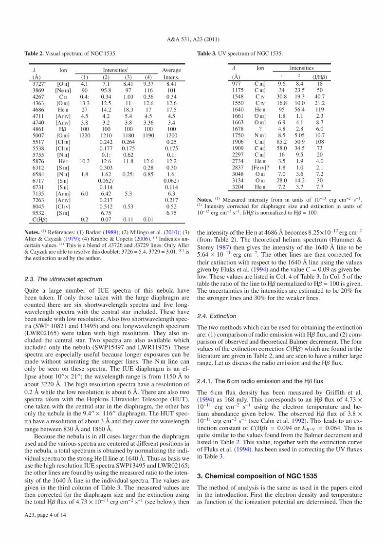
The visual spectrum has been measured by at least six authors.We list here the results from four of these. The line intensitieslisted have been corrected by each author for a value of extinc-tion determined by them to obtain a theoretically correct Balmerdecrement. The result are listed in Table 2, where the last columnlists the average value which we have used. No attempt has beenmade to use a common extinction correction because then theBalmer decrement will be incorrect. The value of extinction Cwhich the individual authors found is listed at the bottom of thetable. None of the spectra measure the weaker lines very well.The errors may be judged by the agreement (or disagreement)of the various measures and appear to be within 20% for thestronger lines and worse for the weaker lines.
Notes. (†) References: (1) Barker (1989); (2) Milingo et al. (2010); (3)Aller & Czyzak (1979); (4) Krabbe & Copetti (2006). (:) Indicates un-certain values. (∗) This is a blend of λ3726 and λ3729 lines. Only Aller& Czyzak are able to resolve this doublet: 3726= 5.4, 3729= 3.01. (C) isthe extinction used by the author.
2.3. The ultraviolet spectrum
Quite a large number of IUE spectra of this nebula havebeen taken. If only those taken with the large diaphragm arecounted there are six shortwavelength spectra and five long-wavelength spectra with the central star included. These havebeen made with low resolution. Also two shortwavelength spec-tra (SWP 10821 and 13495) and one longwavelength spectrum(LWR02165) were taken with high resolution. They also in-cluded the central star. Two spectra are also available whichincluded only the nebula (SWP15497 and LWR11975). Thesespectra are especially useful because longer exposures can bemade without saturating the stronger lines. The N iii line canonly be seen on these spectra. The IUE diaphragm is an el-lipse about 10′′× 21′′; the wavelength range is from 1150 Å toabout 3220 Å. The high resolution spectra have a resolution of0.2 Å while the low resolution is about 6 Å. There are also twospectra taken with the Hopkins Ultraviolet Telescope (HUT),one taken with the central star in the diaphragm, the other hasonly the nebula in the 9.4′′ × 116′′ diaphragm. The HUT spec-tra have a resolution of about 3 Å and they cover the wavelengthrange between 830 Å and 1860 Å.
Because the nebula is in all cases larger than the diaphragmused and the various spectra are centered at different positions inthe nebula, a total spectrum is obtained by normalizing the indi-vidual spectra to the strong He II line at 1640 Å. Thus as basis weuse the high resolution IUE spectra SWP13495 and LWR02165;the other lines are found by using the measured ratio to the inten-sity of the 1640 Å line in the individual spectra. The values aregiven in the third column of Table 3. The measured values arethen corrected for the diaphragm size and the extinction usingthe total Hβ flux of 4.73 × 10⁻¹¹ erg cm−2 s−1 (see below), then
Table 3. UV spectrum of NGC 1535.
λ Ion Intensities
(Å) 1 2 (I/Hβ)977 C iii] 9.6 8.4 181175 C iii] 34 23.5 501548 C iv 30.8 19.3 40.71550 C iv 16.8 10.0 21.21640 He ii 95 56.4 1191661 O iii] 1.8 1.1 2.31663 O iii] 6.9 4.1 8.71678 ? 4.8 2.8 6.01750 N iii] 8.5 5.05 10.71906 C iii] 85.2 50.9 1081909 C iii] 58.0 34.5 732297 C iii] 16 9.5 202734 He ii 3.5 1.9 4.02837 [Fe iv]? 1.8 1.0 2.13048 O iii 7.0 3.6 7.23134 O iii 28.0 14.2 303204 He ii 7.2 3.7 7.7
Notes. (1) Measured intensity from in units of 10−13 erg cm−2 s−1.(2) Intensity corrected for diaphragm size and extinction in units of10−12 erg cm−2 s−1. I/Hβ is normalized to Hβ = 100.
the intensity of the He ii at 4686 Å becomes 8.25×10⁻¹² erg cm−2
(from Table 2). The theoretical helium spectrum (Hummer &Storey 1987) then gives the intensity of the 1640 Å line to be5.64 × 10−11 erg cm−2. The other lines are then corrected fortheir extinction with respect to the 1640 Å line using the valuesgiven by Fluks et al. (1994) and the value C = 0.09 as given be-low. These values are listed in Col. 4 of Table 3. In Col. 5 of thetable the ratio of the line to Hβ normalized to Hβ = 100 is given.The uncertainties in the intensities are estimated to be 20% forthe stronger lines and 30% for the weaker lines.
2.4. Extinction
The two methods which can be used for obtaining the extinctionare: (1) comparison of radio emission with Hβ flux, and (2) com-parison of observed and theoretical Balmer decrement. The fourvalues of the extinction correction C(Hβ) which are found in theliterature are given in Table 2, and are seen to have a rather largerange. Let us discuss the radio emission and the Hβ flux.
2.4.1. The 6 cm radio emission and the Hβ flux
The 6 cm flux density has been measured by Griffith et al.(1994) as 168 mJy. This corresponds to an Hβ flux of 4.73 ×10⁻¹¹ erg cm−2 s−1 using the electron temperature and he-lium abundance given below. The observed Hβ flux of 3.8 ×10⁻¹¹ erg cm−2 s−1 (see Cahn et al. 1992). This leads to an ex-tinction constant of C(Hβ) = 0.094 or EB−V = 0.064. This isquite similar to the values found from the Balmer decrement andlisted in Table 2. This value, together with the extinction curveof Fluks et al. (1994). has been used in correcting the UV fluxesin Table 3.
3. Chemical composition of NGC 1535
The method of analysis is the same as used in the papers citedin the introduction. First the electron density and temperatureas function of the ionization potential are determined. Then the
A23, page 4 of 14
S. R. Pottasch et al.: Abundances in NGC 1535
Table 4. Observed electron density indicators in the nebulae.
Ion Ioniz. Lines Obs. Ratio Ne (cm−3) Obs. Ratio Ne (cm−3) Obs. Ratio Ne (cm−3) Obs. Ratio Ne (cm−3)Pot.(eV) Used NGC 1535 NGC 1535 Tc1 Tc1 He2-108 He2-108 NGC 6629 NGC 6629
Table 5. Observed electron temperature indicators in the nebulae.
Ion Ioniz. Lines Obs. Ratio Te(K) Obs. Ratio Te(K) Obs. Ratio Te(K) Obs. Ratio Te(K)Pot.(eV) Used NGC 1535 NGC 1535 Tc1 Tc1 He2-108 He2-108 NGC 6629 NGC 6629
ionic abundances are determined, using density and tempera-ture appropriate for the ion under consideration, together withEq. (1). Then the element abundances are found for those ele-ments in which a sufficient number of ion abundances have beenderived.
3.1. Electron density
The ions used to determine Ne are listed in the first column ofTable 4. The ionization potential required to reach that ionizationstage, and the wavelengths of the lines used, are given in Cols. 2and 3 of the table. Note that the wavelength units are Å when4 ciphers are given and microns when 3 ciphers are shown. Theobserved ratio of the lines is given in the fourth column; the cor-responding Ne is given in the fifth column. The temperature usedis discussed in the following section, but is unimportant sincethese line ratios are essentially determined by the density.
The electron density appears to be about 1000 cm−3 althoughthe two ions with the lowest ionization potential give a some-what higher value. These values are less well determined be-cause the ratios are poorly measured. The density is probably notuniform as indicated by the structures seen in the central area ofthe nebula, which may contribute to this difference. A density of1000 cm−3 is used in the abundance determination in Table 6,but none of the abundances listed in the table is sensitive to thedensity in the range shown in the table.
3.2. Electron temperature
A number of ions have lines originating from energy levels farenough apart that their ratio is sensitive to the electron tempera-ture. These are listed in Table 5, which is arranged similarly tothe previous table. While there is a slight scatter in these valuesthere is no clear indication of a temperature gradient as functionof the ionization potential as has been seen in some other neb-ulae. An electron temperature of 12 000 K will be used with anuncertainty of less than 1000 K.
3.3. Ionic and element abundances
The ionic abundances have been determined using the followingequation:
Nion
Np=
Iion
IHβNeλul
λHβ
αHβ
Aul
(Nu
Nion
)−1
(1)
where Iion/IHβ is the measured intensity of the ionic line com-pared to Hβ, Np is the density of ionized hydrogen, λul is thewavelength of this line, λHβ is the wavelength of Hβ, αHβ is theeffective recombination coefficient for Hβ, Aul is the Einsteinspontaneous transition rate for the line, and Nu/Nion is the ra-tio of the population of the level from which the line originatesto the total population of the ion. This ratio has been determinedusually using a five level atom. Sometimes a two level atom wassufficient.
The results are given in Table 6, where the first column liststhe ion concerned, and the second column the line used for theabundance determination. The third column gives the intensityof the line used relative to Hβ = 100. The fourth column showsthe ionic abundances, and the fifth column gives the ionizationcorrection factor (ICF). This has been determined empirically,usually by looking at the ionization potential of the missing ion.Notice that the ICF is unity for all elements except for Ar, S andCl where it is close to unity. The helium abundance has beenderived with the help of the theoretical work of Benjamin et al.(1999) and Porter et al. (2005).
3.4. Comparison with other determinations
In Table 7 the present abundances are compared to earlier deter-minations. The agreement is usually within a factor of 2, exceptfor Chlorine which is difficult to measure.
4. Tc1 (IC 1266)
Tc1 (PN G345.2-08.8, also known as IC 1266, SaSt 2-16and IRAS 17418-4604) is morphologically quite similar to
A23, page 5 of 14
A&A 531, A23 (2011)
Table 6. Ionic concentrations and chemical abundances in NGC 1535.
Notes. Wavelength in Angstrom for all values of λ above 1000, oth-erwise in μm. Intensities given with respect to Hβ = 100. (:) Indicatesuncertain values.
NGC 1535. It is roughly circular and has a size at the 10% levelof 12.9′′× 12.2′′(Tylenda et al. 2003). A somewhat smaller di-ameter (9.6′′) is given by Acker et al. (1992). The size is smallenough so that most of the radiation can be measured in the IUEdiaphragm. The nebula is surrounded by a faint halo which isalso circular and has a diameter of about 53′′.
The 6 cm continuum radio flux density has been measuredby Griffith et al. (1994) as 140 mJy. Milne & Aller (1982)have measured the 2 cm radio flux density as 130 mJy, whichcorresponds to a value of 147 mJy at 6 cm. We use an aver-age value of 145 mJy at 6 cm, which corresponds to an Hβflux of 5.1 × 10⁻¹¹ erg cm−2 s−1. The measured Hβ flux is2.18 × 10−11 erg cm−2 s−1 (see Acker et al. 1992) which leadsto an extinction coefficient C = 0.36.
4.1. Infrared spectrum
The IRS measurement of Tc 1 was centered at RA(2000)17h45m35.3s and Dec(2000) −46◦05′23.3′′. This is almost ex-actly the same as the value measured by Kerber et al. (2003)of RA(2000) 17h45m35.3s and Dec(2000) −46◦05′23.8′′, whichis presumably the coordinate of the central star. Thus the IRSmeasurement was well centered on the nebula. The measured
Notes. (†) References; (1) Williams et al. (2008); (2) Kingsburgh et al.(1994). (:) Indicates uncertain values. (C) Is the extinction used by theauthor.
emission line intensities are given in Table 1, after correcting theSH measurements by the factor 2.02 and the SL measurementsby a factor of 2.35, in the column labeled “intensity”. The Hβflux found from the infrared hydrogen lines (especially the linesat 12.37 μm) using the theoretical ratios of Hummer & Storey(1987), is 6.15 × 10⁻¹¹ erg cm−2 s−1, which is about 20% higherthan the total Hβ intensity. This indicates that the LH diaphragmmeasured the entire nebula. The measurement of a higher flux inthe infrared is within the uncertainties of the various measure-ments. Two of the features in the table have been identified asbelonging to the fullerene molecules (Cami 2010).
4.2. Visual spectrum
There are only a few visual spectra of Tc 1. The best is the verygood spectrum reported by Williams et al. (2008). These authorsmeasured the nebula at two positions at either side of the cen-tral star, but carefully avoiding the star. They used a rectangu-lar slit 2′′× 4′′. They correct their intensities for an extinctionfound from the Balmer decrement, These corrected intensitiesare shown in the third column of Table 8 for some of the linesof interest to us. Notice that the [Ne iii] line at λ3869 Å was tooweak to measure. Williams et al. (2008) do not report the inten-sities of any of the He i lines; for the intensities of these linesthe spectrum reported by Kingsburgh & Barlow (1994) are used.These are shown in Col. 4 of the table, where the average inten-sity is weighted to the spectrum of Williams et al. (2008).
4.3. The ultraviolet spectrum
There are 14 IUE spectra of Tc 1: three high resolution short-wave spectra, seven low resolution shortwave spectra and fourlow resolution longwave spectra. Only a few lines are strongenough for a good identification as a nebular line however. Inaddition the spectrum is of low excitation so that the connec-tion between the ultraviolet and visual spectra through the He ii
A23, page 6 of 14
S. R. Pottasch et al.: Abundances in NGC 1535
Table 9. UV spectrum of Tc 1.
λ Ion Intensities(Å) (1) (2) (I/Hβ)1906 C iii] 1.45 7.6 14.81909 C iii] 1.16 6.1 11.92325 C ii] 3.90 23.4 45.5
Notes. (1) Measured intensity from in units of 10−12 erg cm−2 s−1.(2) Intensity corrected for extinction in units of 10−12 erg cm−2 s−1. I/Hβis normalized to Hβ = 100.
lines of λ1640 Å and λ4686 Å cannot be made. However thenebula is small enough so that almost all of its emission is mea-sured. Feibelman (1983) has reported measuring the [O ii] line atλ2471 Å which can be used to connect the ultraviolet spectrumto the visual spectrum but we feel that the spectra are too noisyto measure this line. We find that only two lines are clearly mea-surable on the low resolution spectra. The high resolution spectrashows more lines but because they may be interstellar or stellarwe do not report them here. Table 9 lists our measurements. Theextinction correction is made using a value of C = 0.33 as foundby Williams et al. (2008).
4.4. Electron density
The ions used to determine Ne are listed in the first columnof Table 4. The corresponding electron density is given inColumn 7. It is about 3000 cm−3.
4.5. Electron temperature
Five ions have lines originating from energy levels far enoughapart that their ratio is sensitive to the electron temperature.These are listed in Table 5. An electron temperature of 9000 Kwill be used with an uncertainty of less than 500 K.
4.6. Ionic and element abundances
The ionic abundances have been determined using Eq. (1)above with an electron temperature of 9000 K and a density of3000 cm−3. The results are given in Table 10, where the firstcolumn lists the ion concerned, the second column the line usedfor the abundance determination and the third column gives theintensity of the line used relative to Hβ = 100. The fourth col-umn shows the ionic abundances, and the fifth column gives theIonization Correction Factor (ICF), determined with the help ofthe model described below. In all cases when the ICF is greaterthan 1, the principal ionization stage of that element has beenobserved.
5. He2-108
He2-108 (PN G316.1+08.4, also known as IRAS 14147-5156)is morphologically quite similar to NGC 1535 and Tc 1. It isroughly circular and has a size at the 10% level of 13.6′′×12.3′′ (Tylenda et al. 2003). A somewhat smaller diameter (11′′)is given by Acker et al. (1992). The size is small enough so thatmost of the radiation can be measured in the IUE diaphragm.
The 6 cm continuum radio flux density has been measuredby Milne & Aller (1975) as 33 mJy. Milne & Aller (1982)have measured the 2 cm radio flux density as 43 mJy, whichcorresponds to a value of 49 mJy at 6 cm. An uncertain av-
Table 10. Ionic concentrations and chemical abundances in Tc 1.
Notes. Wavelength in Angstrom for all values of λ above 1000, other-wise in μm. Intensities given with respect to Hβ = 100.
erage value of 39 mJy at 6 cm corresponds to an Hβ flux of1.26 × 10−11 erg cm−2 s−1. The measured Hβ flux is 3.7 ×10⁻¹² erg cm−2 s−1 (see Acker et al. 1992) which leads to anextinction coefficient C = 0.53.
5.1. Infrared spectrum
The IRS measurement of He2-108 was centered at RA(2000)14h18m08.4s and Dec(2000) −52◦10′38.0′′. This is a slight mis-pointing from the center measured by Kerber et al. (2003) ofRA(2000) 14h18m08.89s and Dec(2000)−52◦10′39.7′′, which ispresumably the coordinate of the central star. This does not havean important effect for the LH measurement because of the largeLH diaphragm. It does however affect the SH measurement forwhich the Nod 1 measurement measured only part of the nebula.The Nod 2 measurement fell within the nebula so that we haveonly used the Nod 2 measurement. By equating the continuummeasured at 19 μm in the LH measurement with the same contin-uum measured in the SH Nod 2 we obtain a ratio of LH/SH= 2.5.The ratio of SH to SL was obtained by equating the [Ne ii] fluxesin the two measurements. All fluxes were measured using theGaussian line-fitting routine. The measured emission line inten-sities are given in Table 1, after correcting the SH measurementsby the factor 2.5 and the SL measurements by a factor of 4.07.The Hβ flux found from the infrared hydrogen lines (especiallythe lines at 7.48 μm and 12.37 μm) using the theoretical ratios ofHummer & Storey (1987), is 1.15×10⁻¹¹ erg cm−2 s−1, which isonly slighly smaller than the Hβ found from the radio flux den-sity. This indicates that the LH diaphragm measured almost theentire nebula.
5.2. Visual spectrum
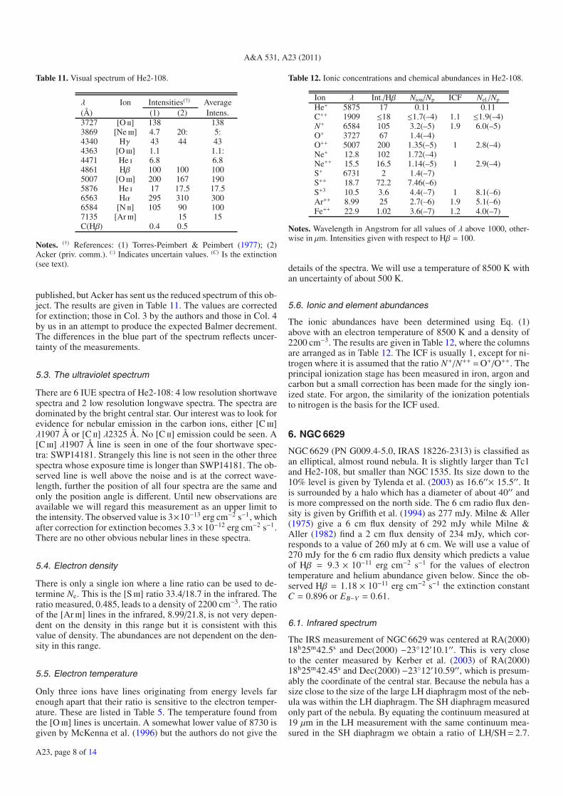
There are two measurements of the visual spectrum of He2-108, probably because it is weak and not visible to northern ob-servatories. The measurements by Torres-Peimbert & Peimbert(1977) are considered by these authors to be less accurate thanmeasurements of other PNe they have made. An accuracy ofabout 30% is given by these authors. The visual spectrum hasalso been measured in the 1990 Acker-Stenholm ESO survey ofsouthern PNe. The full results of this survey have not yet been
Notes. (†) References: (1) Torres-Peimbert & Peimbert (1977); (2)Acker (priv. comm.). (:) Indicates uncertain values. (C) Is the extinction(see text).
published, but Acker has sent us the reduced spectrum of this ob-ject. The results are given in Table 11. The values are correctedfor extinction; those in Col. 3 by the authors and those in Col. 4by us in an attempt to produce the expected Balmer decrement.The differences in the blue part of the spectrum reflects uncer-tainty of the measurements.
5.3. The ultraviolet spectrum
There are 6 IUE spectra of He2-108: 4 low resolution shortwavespectra and 2 low resolution longwave spectra. The spectra aredominated by the bright central star. Our interest was to look forevidence for nebular emission in the carbon ions, either [C iii]λ1907 Å or [C ii] λ2325 Å. No [C ii] emission could be seen. A[C iii] λ1907 Å line is seen in one of the four shortwave spec-tra: SWP14181. Strangely this line is not seen in the other threespectra whose exposure time is longer than SWP14181. The ob-served line is well above the noise and is at the correct wave-length, further the position of all four spectra are the same andonly the position angle is different. Until new observations areavailable we will regard this measurement as an upper limit tothe intensity. The observed value is 3×10⁻¹³ erg cm−2 s−1, whichafter correction for extinction becomes 3.3× 10⁻¹² erg cm−2 s−1.There are no other obvious nebular lines in these spectra.
5.4. Electron density
There is only a single ion where a line ratio can be used to de-termine Ne. This is the [S iii] ratio 33.4/18.7 in the infrared. Theratio measured, 0.485, leads to a density of 2200 cm−3. The ratioof the [Ar iii] lines in the infrared, 8.99/21.8, is not very depen-dent on the density in this range but it is consistent with thisvalue of density. The abundances are not dependent on the den-sity in this range.
5.5. Electron temperature
Only three ions have lines originating from energy levels farenough apart that their ratio is sensitive to the electron temper-ature. These are listed in Table 5. The temperature found fromthe [O iii] lines is uncertain. A somewhat lower value of 8730 isgiven by McKenna et al. (1996) but the authors do not give the
Table 12. Ionic concentrations and chemical abundances in He2-108.
Notes. Wavelength in Angstrom for all values of λ above 1000, other-wise in μm. Intensities given with respect to Hβ = 100.
details of the spectra. We will use a temperature of 8500 K withan uncertainty of about 500 K.
5.6. Ionic and element abundances
The ionic abundances have been determined using Eq. (1)above with an electron temperature of 8500 K and a density of2200 cm−3. The results are given in Table 12, where the columnsare arranged as in Table 12. The ICF is usually 1, except for ni-trogen where it is assumed that the ratio N+/N++ =O+/O++. Theprincipal ionization stage has been measured in iron, argon andcarbon but a small correction has been made for the singly ion-ized state. For argon, the similarity of the ionization potentialsto nitrogen is the basis for the ICF used.
6. NGC 6629
NGC 6629 (PN G009.4-5.0, IRAS 18226-2313) is classified asan elliptical, almost round nebula. It is slightly larger than Tc1and He2-108, but smaller than NGC 1535. Its size down to the10% level is given by Tylenda et al. (2003) as 16.6′′× 15.5′′. Itis surrounded by a halo which has a diameter of about 40′′ andis more compressed on the north side. The 6 cm radio flux den-sity is given by Griffith et al. (1994) as 277 mJy. Milne & Aller(1975) give a 6 cm flux density of 292 mJy while Milne &Aller (1982) find a 2 cm flux density of 234 mJy, which cor-responds to a value of 260 mJy at 6 cm. We will use a value of270 mJy for the 6 cm radio flux density which predicts a valueof Hβ = 9.3 × 10⁻¹¹ erg cm−2 s−1 for the values of electrontemperature and helium abundance given below. Since the ob-served Hβ = 1.18 × 10⁻¹¹ erg cm−2 s−1 the extinction constantC = 0.896 or EB−V = 0.61.
6.1. Infrared spectrum
The IRS measurement of NGC 6629 was centered at RA(2000)18h25m42.5s and Dec(2000) −23◦12′10.1′′. This is very closeto the center measured by Kerber et al. (2003) of RA(2000)18h25m42.45s and Dec(2000) −23◦12′10.59′′, which is presum-ably the coordinate of the central star. Because the nebula has asize close to the size of the large LH diaphragm most of the neb-ula was within the LH diaphragm. The SH diaphragm measuredonly part of the nebula. By equating the continuum measured at19 μm in the LH measurement with the same continuum mea-sured in the SH diaphragm we obtain a ratio of LH/SH= 2.7.
Notes. (†) References; (1) Milingo et al. (2002a); (2) Aller & Keyes.(1987). (:) Indicates uncertain values. (C) Is the extinction (see text).
This number is somewhat uncertain because the spectrum israther noisy. This ratio can also be obtained by comparing boththe [Ne iii] 15.5/36.0 line ratio and the [Ar iii] 21.8/8.99 line ratiosince both of these ratios have only a small dependence in elec-tron density and temperature. We obtain an LH/SH ratio of 1.71from the [Ne iii] lines and a value of 2.44 from the [Ar iii] lines.An average value of LH/SH= 2.1 was used. The ratio of SH toSL was obtained by equating the [Ne ii] the [S iv] fluxes in thetwo measurements which leads to SH/SL= 1.10. All fluxes weremeasured using the Gaussian line-fitting routine.The measuredemission line intensities are given in Table 1, after correcting theSH measurements by the factor 2.1 and the SL measurements bya factor of 2.3. The Hβ flux found from the infrared hydrogenlines (especially the lines at 7.48 μm and 12.37 μm) using thetheoretical ratios of Hummer & Storey (1987) at a temperatureof 8600 K is 8.45 × 10⁻¹¹ erg cm−2 s−1, which is only slighlysmaller than the Hβ found from the radio flux density. This indi-cates that the LH diaphragm measured most of the nebula.
6.2. Visual spectrum
There are several measurements of the visual spectrum ofNGC 6629 in the literature. The two measurements quoted hereare probably the best. These are those of Milingo et al. (2002a)and Aller & Keyes (1987) and are given in Table 13. In addi-tion Kingsburgh & English (1992) have measured the [O ii] ratio3726/3729 to be 1.63± 0.50 and the [S ii] ratio 6717/6731 to be0.74± 0.04.
The extinction coeficients, C, found from the Balmer decre-ment and given at the bottom of the table, are essentially thesame as that found from the radio flux density (given at the be-ginning of this section).
6.3. The ultraviolet spectrum
There are seven IUE spectra of NGC 6629: three low resolutionshortwave spectra and four low resolution longwave spectra. Thediaphragm was centered near the edge of the nebula for some
Table 14. Ionic concentrations and chemical abundances in NGC 6629.
Notes. Wavelength in Angstrom for all values of λ above 1000, other-wise in μm. Intensities given with respect to Hβ = 100.
of the spectra and closer to the central star for other spectra.All spectra appear to be dominated by the bright central star.This indicates that much of the nebula is within the diaphragmbut it is difficult to specify exactly how much of the nebula isbeing measured. The only clearly nebular emission is the [C iii]λ1907 Å line which is seen in all three shortwave spectra. Ithas the same intensity in all spectra: 2.5 × 10⁻¹³ erg cm−2 s−1.Corrected for extinction this becomes 2.2 × 10⁻¹¹ erg cm−2 s−1;thus the ratio of the line to Hβ is 23.7 (when Hβ = 100). Thisvalue will be used when determining the carbon abundance butit is a lower limit since some of the nebular emission may beoutside the nebula. Possible [C ii] λ2325 Å cannot be seen.
6.4. Electron density
The ions used to determine Ne are listed Table 4. The electrondensity appears to be about 2000 cm−3.
6.5. Electron temperature
Four ions have lines originating from energy levels far enoughapart that their ratio is sensitive to the electron temperature.These are listed in Table 5. An electron temperature of 8700 Kis found with an uncertainty of less than 300 K. No temperaturegradient is apparent.
6.6. Ionic and element abundances
The ionic abundances have been determined using Eq. (1)above with an electron temperature of 8700 K and a densityof 2000 cm−3. The results are given in Table 14, where, as inTable 6, the first column lists the ion concerned, the second col-umn the line used for the abundance determination and the thirdcolumn gives the intensity of the line used relative to Hβ = 100.The fourth column shows the ionic abundances, and the fifth col-umn gives the Ionization Correction Factor (ICF), determinedempirically. In all cases but one, when the ICF is greater than1, the principal ionization stage of that element has been ob-served. The single exception is nitrogen, where it is assumedthat N+/N++ =O+ /O++.
A23, page 9 of 14
A&A 531, A23 (2011)
6.7. Errors
We refer here to possible abundance errors in all of the PNestudied here. This is difficult to specify because there are errorsdue to the measurements, the electron temperature and the ICF.There is only a neglible error due to uncertainties in the elec-tron density. The measurement error depends on the strength ofthe line; for the stronger lines it is probably less than 15%. Thevalues of Te appear to be independent of the ionization poten-tial in all PNe considered here. For at least two of the nebulaethe uncertainty could be as large as 1000 K. The temperatureuncertainty plays only a small role for the infrared lines but ismuch more important for the ultraviolet lines. Taken togetherwe estimate that for all elements except carbon the abundanceuncertainties are not more than 20–30% for those elements forthe ICF is close to unity. When the ICF is higher than 1.5 theabundance uncertainties are about 50%. For carbon the ICF isusually unity but the abundance is very temperature dependent.The error is probably slightly higher, of the order of 50% for thiselement. The largest error for helium occurs in the PNe with lowtemperature central stars where neutral helium is present. Thisoccurs in Tc1, but may also occur in NGC 6629 and He2-108.Other sources of error for the helium abundance are probablysmall.
7. Model
In order to obtain as nearly a correct model as possible, the staras well as the nebula must be considered. Modeling the nebula-star complex will allow characterizing not only the central star’stemperature but other stellar parameters as well (i.e., log g andluminosity). It can determine distance and other nebular proper-ties, especially the composition, including the composition ofelements that are represented by a single stage of ionization,which cannot be determined by the simplified analysis above.This method can take the presence of dust and molecules intoaccount in the nebular material, when there is any there, makingit a very comprehensive approach. While the line ratio methodis simple and fast, the ICFs rest on uncertain physics. To thisend, modeling serves as an effective means, and the whole set ofparameters are determined in a unified way, assuring self con-sistency. Also, in this way one gets good physical insight intothe PN, the method and the observations. Thus, modeling is agood approach to an end-to-end solution to the problem. We usedCloudy version C08.00 for this work.
7.1. Tc1
7.1.1. Assumptions
Tylenda et al. (2003) give a diameter of 12.9′′ × 12.2′′ for thisPN. We have used a diameter of 12.55′′ in our modeling.
7.1.2. Model results
Numerous models were run and we found that there was the pri-mary problem of fixing the stellar effective temperature. Whilethe ionization of carbon, neon and argon indicated a somewhatlower Teff, the observed [O iii] lines required a higher value. Wetried a range of temperatures, distances, densities, density pro-files and various model atmospheres. Some models have beentried with stellar wind and some without while some with sim-ple black body atmospheres for the CSPN. Observed [O iii] linefluxes seem to be unusually high and in trying to match them, Ne
Table 15. Parameters representing the final model for Tc1.
Parameter ValueIonizing sourceModel atmosphere WMbasicTeff 34 700 KLog g 3.30Log z –0.3Luminosity 1480 L�
Nebula
Density profile constant density 2850/ccAbundance H He C N
12.000 10.916 8.674 7.590O Ne Mg Si
8.431 7.481 5.5 5.778P S Cl Ar5.3 6.203 4.963 6.478
Size 6.275′′ (radius)Distance 1.80 kpcDust grains Graphites of single size 1.0 μm;inner radius 1.077e16 cmouter radius 1.690e17 cmFilling factor 1.0
and Ar moved up to higher stages of ionization. Many observedlines would suggest a cooler Teff than what our final model in-dicated. In the final model, shown in Table 15, we have used alow metallicity model atmosphere mainly to take care of infus-ing more photons in the wavelength region below 912 Å withoutincreasing Teff . The metallicity is only half that of Sun. The valueof gravity was also kept as low as possible for a similar boost inthe input stellar radiation. We note that the galactic latitude ofthe CSPN is only around −9 degrees and the fact that we wereforced to use a low metallicity model atmosphere for such a lowlatitude object shows the extreme to which a modeler is driven,when faced with anomalous nebular line emission.
At this stage we were not sure whether any extra source ofenergy was present, as there was no observational clue, but theabove facts forced us to look at all different possibilities. It mightas well be that model atmospheres do not realistically representthe stellar radiation. Another fact is that the accuracy of the op-tical spectra containing the O iii lines is quite high, an error ofonly 8% is quoted by the authors for the spectrophotometry.Therefore we surmise that something very interesting is happen-ing in the formation of O iii lines but are unable to hazard anyguess. But while we did these adjustments in modeling, lines ofneon, argon and sulphur gave trouble. The sulphur lines wereimproved to get a better fit by adjusting the DR (dielectronicrecombination) rates since the DR rates are poorly known. Thefinal model output spectra are presented in Table 16, where it isclear that the model fluxes for most low ionization stages (O ii,C ii, and Ne ii) are too high.
To reproduce the observed IR dust continua, we found thatgraphites gave a better fit and used them in our modeling ratherthan silicates. The grains included in the modeling were theCloudy’s set called Orion distribution which has a bias towardslarger grain sizes. The match to the observed IR continua is rea-sonable (see Fig. 1). So the final model we present is the best wecould achieve. Overall we feel our exercise raises more pertinentquestions than answers as this PN seems to throw lots of chal-lenges to our current understanding of nebular physics. We areinclined to recommend the abundances as determined by the ICFmethod for this PN. A very pertinent point we want to highlight
A23, page 10 of 14
S. R. Pottasch et al.: Abundances in NGC 1535
Table 16. The emission line fluxes (Hβ = 100) for Tc1.
Label Line† Model flux Obsd. flux Label Line Model flux Obsd. flux(dereddened) (dereddened)
TOTL 4861A 100.00 100.00 S 3 6312A 0.40 0.46C 2 1335A 10.35 11.43 O 1 6363A 0.78 0.05C 3 1478A 0.00 6.65 N 2 6548A 32.43 30.10C 1 1561A 0.34 1.26 N 2 6584A 95.70 93.20C 2 1761A 0.18 2.08 S II 6716A 2.38 2.15C 3 1907A 16.56 14.76 S II 6731A 3.70 3.41C 3 1910A 11.85 11.94 Ar 3 7135A 15.52 6.99TOTL 2326A 86.80 44.59 O II 7323A 9.04 5.43O II 3726A 171.42 131.10 O II 7332A 7.23 4.57O II 3729A 91.40 86.59 Ar 3 7751A 3.74 1.66S II 4070A 0.84 0.62 Fe 2 8617A 0.02 0.01S II 4078A 0.27 0.18 C 1 8727A 0.05 0.01Fe 2 4244A 0.00 0.02 S 3 9069A 7.64 12.51Fe 2 4359A 0.00 0.01 TOTL 9850A 0.54 0.04TOTL 4363A 0.53 0.56 Ar 2 6.980m 14.12 32.84P 2 4669A 0.02 0.01 Ar 3 9.000m 16.23 6.49O 3 4959A 40.50 41.71 S 4 10.51m 0.51 0.47O 3 5007A 121.92 123.00 Ne 2 12.81m 19.68 37.41Ar 3 5192A 0.08 0.03 Ne 3 15.55m 3.24 1.46N 1 5198A 0.16 0.02 P 3 17.89m 0.72 0.73N 1 5200A 0.06 0.02 S 3 18.67m 12.47 14.03Cl 3 5518A 0.27 0.28 Ar 3 21.83m 1.05 0.43Cl 3 5538A 0.29 0.30 Fe 3 22.92m 0.27 0.29O 1 5577A 0.04 0.00 S 3 33.47m 4.77 6.21N 2 5755A 1.23 1.08 Si 2 34.81m 0.32 0.30O 1 6300A 2.45 0.12
Notes. Absolute Hβ flux model: 5.83 × 10⁻¹¹ erg cm−2 s−1 Obsn: 6.15 × 10⁻¹¹ ergs cm−2 s−1. “A” in Col. “Line” signifies Angstrom; “m” signifiesμm. In col. “Label”, we have followed the notation used by Cloudy for atoms and ions; this will make identifying a line in Cloudy’s huge line listeasy. Neutral state is indicated by “1” and singly ionized state by “2” etc., “TOTL” typically means the sum of all the lines in the doublet/multiplet;or it could mean sum of all processes: recombination, collisional excitation, and charge transfer. Some elements are represented by usual notationas per Cloudy.
Fig. 1. The IR dust continua of Tc1 . The asterisks represent the obser-vation from Spitzer and the continuous curve is the model output.
is the fact that this PN shows nebular absorption lines too; seeWilliams et al. (2008) and to the best of our knowledge exist-ing photoionization codes are yet to have a provision for com-puting the equivalent widths of such lines so that they can alsobe compared with observed values. This would make the crite-ria for a good fit (with observation) more stringent. Presentlyall models published till date used only nebular emission linesalone. Incorporating the formation of absorption lines would bethe next major paradigm shift in photoionization modeling.
7.2. Modeling NGC 1535
We now describe our unsuccessful efforts to make a photoion-ization model for this PN. It is necessary to go into the detailssince it reveals insights into aspects of nebular physics which arenormally taken for granted as well known.
7.2.1. Assumptions
The appearance of NGC 1535 from an image taken by Schwarzet al. (1992) is nearly spherical. The IR and radio measurementsdescribed earlier give an absolute Hβ flux that is consistent witha diameter of 45′′, that includes a low density outer zone be-yond a high density innerzone of diameter of 19′′. We wantedto include a density profile for the nebula to describe the varia-tion of the number density N(H) with the radius and so derived atemplate profile from the Hα image taken from http://astro.uni-tuebingen.de/groups/pn/. The image was taken on anas-is basis and imported into the IRAF and using cross-cuts atdifferent azimuths an average profile was generated and then nor-malized to have a peak value of 1300/cc. The nebular radius wasnormalized to 22.5′′, to include the low density region as well.We used this profile as a starting value but later have experi-mented with modifications to it as well as tried simple constantdensity models. Though the presence of dust and H2 moleculesis observed in this PN we did not include them in our simula-tions.
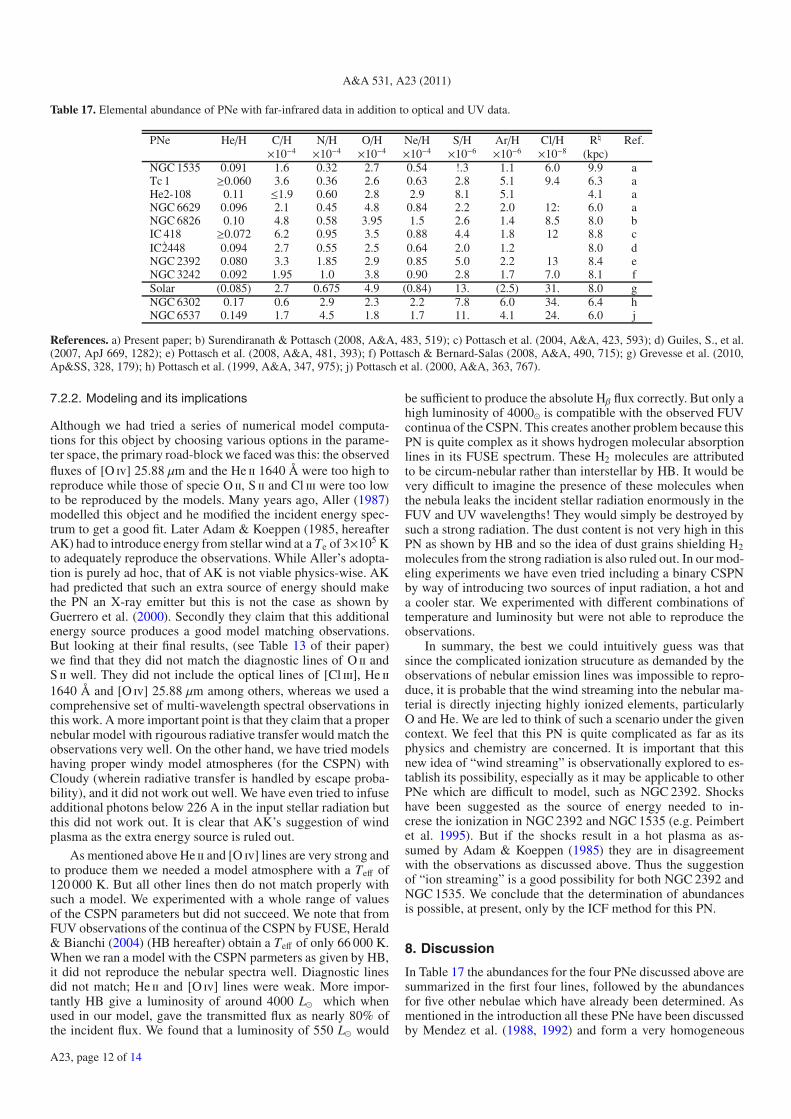
References. a) Present paper; b) Surendiranath & Pottasch (2008, A&A, 483, 519); c) Pottasch et al. (2004, A&A, 423, 593); d) Guiles, S., et al.(2007, ApJ 669, 1282); e) Pottasch et al. (2008, A&A, 481, 393); f) Pottasch & Bernard-Salas (2008, A&A, 490, 715); g) Grevesse et al. (2010,Ap&SS, 328, 179); h) Pottasch et al. (1999, A&A, 347, 975); j) Pottasch et al. (2000, A&A, 363, 767).
7.2.2. Modeling and its implications
Although we had tried a series of numerical model computa-tions for this object by choosing various options in the parame-ter space, the primary road-block we faced was this: the observedfluxes of [O iv] 25.88 μm and the He ii 1640 Å were too high toreproduce while those of specie O ii, S ii and Cl iii were too lowto be reproduced by the models. Many years ago, Aller (1987)modelled this object and he modified the incident energy spec-trum to get a good fit. Later Adam & Koeppen (1985, hereafterAK) had to introduce energy from stellar wind at a Te of 3×10⁵ Kto adequately reproduce the observations. While Aller’s adopta-tion is purely ad hoc, that of AK is not viable physics-wise. AKhad predicted that such an extra source of energy should makethe PN an X-ray emitter but this is not the case as shown byGuerrero et al. (2000). Secondly they claim that this additionalenergy source produces a good model matching observations.But looking at their final results, (see Table 13 of their paper)we find that they did not match the diagnostic lines of O ii andS ii well. They did not include the optical lines of [Cl iii], He ii1640 Å and [O iv] 25.88 μm among others, whereas we used acomprehensive set of multi-wavelength spectral observations inthis work. A more important point is that they claim that a propernebular model with rigourous radiative transfer would match theobservations very well. On the other hand, we have tried modelshaving proper windy model atmospheres (for the CSPN) withCloudy (wherein radiative transfer is handled by escape proba-bility), and it did not work out well. We have even tried to infuseadditional photons below 226 A in the input stellar radiation butthis did not work out. It is clear that AK’s suggestion of windplasma as the extra energy source is ruled out.
As mentioned above He ii and [O iv] lines are very strong andto produce them we needed a model atmosphere with a Teff of120 000 K. But all other lines then do not match properly withsuch a model. We experimented with a whole range of valuesof the CSPN parameters but did not succeed. We note that fromFUV observations of the continua of the CSPN by FUSE, Herald& Bianchi (2004) (HB hereafter) obtain a Teff of only 66 000 K.When we ran a model with the CSPN parmeters as given by HB,it did not reproduce the nebular spectra well. Diagnostic linesdid not match; He ii and [O iv] lines were weak. More impor-tantly HB give a luminosity of around 4000 L� which whenused in our model, gave the transmitted flux as nearly 80% ofthe incident flux. We found that a luminosity of 550 L� would
be sufficient to produce the absolute Hβ flux correctly. But only ahigh luminosity of 4000� is compatible with the observed FUVcontinua of the CSPN. This creates another problem because thisPN is quite complex as it shows hydrogen molecular absorptionlines in its FUSE spectrum. These H2 molecules are attributedto be circum-nebular rather than interstellar by HB. It would bevery difficult to imagine the presence of these molecules whenthe nebula leaks the incident stellar radiation enormously in theFUV and UV wavelengths! They would simply be destroyed bysuch a strong radiation. The dust content is not very high in thisPN as shown by HB and so the idea of dust grains shielding H2molecules from the strong radiation is also ruled out. In our mod-eling experiments we have even tried including a binary CSPNby way of introducing two sources of input radiation, a hot anda cooler star. We experimented with different combinations oftemperature and luminosity but were not able to reproduce theobservations.
In summary, the best we could intuitively guess was thatsince the complicated ionization strucuture as demanded by theobservations of nebular emission lines was impossible to repro-duce, it is probable that the wind streaming into the nebular ma-terial is directly injecting highly ionized elements, particularlyO and He. We are led to think of such a scenario under the givencontext. We feel that this PN is quite complicated as far as itsphysics and chemistry are concerned. It is important that thisnew idea of “wind streaming” is observationally explored to es-tablish its possibility, especially as it may be applicable to otherPNe which are difficult to model, such as NGC 2392. Shockshave been suggested as the source of energy needed to in-crese the ionization in NGC 2392 and NGC 1535 (e.g. Peimbertet al. 1995). But if the shocks result in a hot plasma as as-sumed by Adam & Koeppen (1985) they are in disagreementwith the observations as discussed above. Thus the suggestionof “ion streaming” is a good possibility for both NGC 2392 andNGC 1535. We conclude that the determination of abundancesis possible, at present, only by the ICF method for this PN.
8. Discussion
In Table 17 the abundances for the four PNe discussed above aresummarized in the first four lines, followed by the abundancesfor five other nebulae which have already been determined. Asmentioned in the introduction all these PNe have been discussedby Mendez et al. (1988, 1992) and form a very homogeneous
A23, page 12 of 14
S. R. Pottasch et al.: Abundances in NGC 1535
Table 18. Prediction of central star mass and distance from evolution theory.
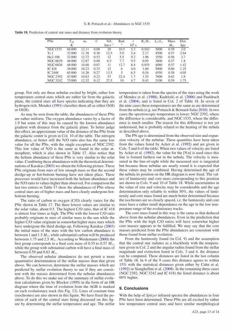
PNe Teff mv C Vel. Rad. t Rs/R� Ls/L� Mass Dist.K km s−1 ′′ 103 s M� kpc
group. Not only are these nebulae excited by bright, rather lowtemperature central stars which are rather far from the galacticplane, the central stars all have spectra indicating that they arehydrogen rich. Mendez (1991) classifies them all as either O(H)or Of(H).
As may be seen from the table, the abundances of these PNeare rather uniform. The oxygen abundance varies by a factor of1.9 but some of this may be caused by the known abundancegradient with distance from the galactic plane. To better judgethis effect, an approximate value of the distance of the PNe fromthe galactic center is given in Col. 10 of the table. The nitrogenabundance, or better still the N/O ratio also has the same lowvalue for all the PNe, with the single exception of NGC 2392.This low value of N/O is the same as found in the solar at-mosphere, which is also shown in Table 17. Also notice thatthe helium abundance of these PNe is very similar to the solarvalue. Combining these abundances with the theoretical determi-nations of Karakas (2003) we obtain the following picture. ThesePNe originate from stars of low enough mass so that the seconddredge-up or hot-bottom burning have not taken place. Theseprocesses would have increased both the helium abundance andthe N/O ratio to values higher than observed. For comparison thelast two entries in Table 17 show the abundances of PNe whosecentral stars are of higher mass and have clearly undergone hot-bottom burning.
The ratio of carbon to oxygen (C/O) clearly varies for thePNe shown in Table 17. The three lowest values are similar tothe solar value, about 0.5. The highest C/O ratio, that of IC 418is almost four times as high. The PNe with the lowest C/O ratioprobably originate in stars of similar mass to the sun while thehigher C/O value originate in somewhat higher mass stars whichhave undergone the third dredge-up. Following Karakas (2003)the initial mass of the stars with the low carbon abundance isbetween 1 and 1.5 M�, while substantial carbon will be producedbetweem 1.75 and 2.5 M�. According to Weidemann (2000) thefirst group corresponds to a final core mass of 0.55 to 0.57 M�,while the group with substantial carbon will have a final mass ofbetween 0.59 and 0.63 M�.
The observed nebular abundances do not permit a morequantitative determination of the stellar masses than that givenabove. We can however, determine the stellar masses which arepredicted by stellar evolution theory to see if they are consis-tent with the masses determined from the nebular abundancesabove. To do this we make use of the summary of stellar evolu-tion calculations given by Blocker (1995) in the form of an HRdiagram where the time of evolution from the AGB is markedon each evolutionary track (his Fig. 12). Lines of constant time(isochrones) are also shown in this figure. We have fixed the po-sition of each of the central stars being discussed on this fig-ure by determining the stellar temperature and age. The stellar
temperature is taken from the spectra of the stars using the workof Mendez et al. (1988), Kudritzki et al. (2006) and Pauldrachet al. (2004), and is listed in Col. 2 of Table 18. In seven ofthe nine cases these temperatures are the same as are determinedfrom the nebula (e.g. see Pottasch & Bernard-Salas 2010). In twocases the spectroscopic temperature is lower: NGC 2392, wherethe difference is considerable, and NGC 1535, where the differ-ence is much smaller. The reason for this difference is not yetunderstood, but is probably related to the heating of the nebulaas described above.
The PN age is determined from the observed size and expan-sion velocity of the nebulae. These quantities have been takenfrom the values listed by Acker et al. (1992) and are given inCols. 5 and 6 of the table. When two values of velocity are listedby Acker et al. (1992), the value for the [N ii] is used since thisline is formed farthest out in the nebula. The velocity is mea-sured in the line-of-sight while the measured size is tangentialbut because these nebulae are nearly round it is expected thatthese values may be combined. Having determined the age ofthe nebula its position on the HR diagram is now fixed. The val-ues of luminosity and core mass corresponding to this positionare shown in Cols. 9 and 10 of Table 18. While uncertainties inthe value of size and velocity may be considerable and the agedetermination only reliable to within 50%, the values of lumi-nosity and core mass found are much better determined becausethe isochrones are so closely spaced, i.e. the luminosity and coremass have a rather small dependance on the age in the low tem-perature range of the evolutionary tracks.
The core mass found in this way is the same as that deducedabove from the nebular abundances. Even in the prediction thatthe PNe with the high C/O ratios will have somewhat highercore masses appears to be fulfilled. We may say that the coremasses predicted from the PNe abundances are consistent withthose found from stellar evolution.
From the luminosity found (in Col. 9) and the assumptionthat the central star radiates as a blackbody with the tempera-ture given in Col. 2 and the angular radius found from the stellarmagnitude and extinction listed in Cols. 3 and 4, the distancecan be computed. These distances are listed in the last columnof Table 18. In 6 of the 9 cases this distance agrees to within15% with the statistical distances given either by Cahn et al.(1992) or Stanghellini et al. (2008). In the remaining three cases(NGC 2392, NGC 3242 and IC 418) the listed distance is about60% higher.
9. Conclusions
With the help of Spitzer infrared spectra the abundances in fourPNe have been determined. These PNe are all excited by ratherlow temperature central stars and have similar morphological
A23, page 13 of 14
A&A 531, A23 (2011)
and kinematic properties: they are all nearly round and are ratherfar from the galactic plane. We are able to show that these nebu-lae have rather similar abundances of helium, oxygen, nitrogen,carbon and other elements. The resultant abundances are sum-marized in the first four lines of Table 17. We then show thatfive other PNe with low temperature central whose abundanceshave been determined using Spitzer infrared spectra and havethe same or similar morphological and kinematic properties alsohave the same or similar abundances.
By comparing these abundances with those predicted by nu-cleosynthesis models by Karakas (2003) it is deduced that thesePNe originate from stars of initial mass between 1 M� and about2.5 M�, which according to Weidemann (2000) correspond tocore masses of between 0.56 M� and 0.63 M�. These values ofcore masses are compared with those determined from stellarevolution theory using the observed temperature of the centralstar and the measured age of the nebula. The core masses thusfound are consistent with each other. Two details reinforce thisconsistency. First, the higher core masses from the evolutionarytheory are found in PNe which have high C/O abundance ratiosas the models of Karakas (2003) predict. Secondly the distancesfound from the stellar evolution are in general values expectedfrom statistical distance scales.
There are a number of uncertainties which must still be con-sidered. First, it is not understood why the central star temper-ature measured in NGC 2392 is so much lower than that foundfrom the nebula. Second, distances found by some researchersare different than found here. For example, the distances givenby Kudritzki et al. (2006) for 6 of the PNe listed are 50% higherthan we have found. This could be due to errors in their de-termination of the stellar gravity from uncertain line profiles.Furthermore the expansion distances found for two of the nebu-lae (NGC 3242 and IC 2448) are at least a factor of 2 lower thanwe have found here. This should be carefully considered in thefuture.
Acknowledgements. We duly acknowledge the use of SIMBAD and ADS in thisresearch work. We have used the IUE spectra archive at the STSCI and we wishto thank the archive unit for the same. R.S. would like to acknowledge that apart of his research work was done when he was working at the Indian Inst.of Astrophysics, Bangalore. R.S. sincerely thanks his former colleagues J. S.Nathan and B. A. Varghese for help with S/W upgradation.
References
Acker, A., Marcout, J., Ochsenbein, F., et al. 1992, Strasbourg-ESO catalogueAdams, J., & Koppen, J. 1985, A&A, 142, 461Aller, L. H. 1982, Ap&SS, 83, 225Aller, L. H., & Czyzak, S. J. 1979, Ap&SS, 62.397Aller, L. H., & Keyes, C. D. 1987, ApJS, 65, 405Banerjee, D. P. K., & Anandaro, B. G. 1991, A&A, 250, 165Barker, T. 1989, ApJ, 340, 421Benjamin, R. A., Skillman, E. D., & Smits, D. P. 1999, ApJ, 514, 307Bernard Salas, J., Pottasch, S. R., Beintema, D. A., & Wesselius, P. R. 2001,
A&A, 367, 949Blocker, T. 1995, A&A, 299, 755Cahn, J. H., Kaler, J. B., & Stanghellini, L. 1992, A&AS, 94, 399Cami, J., Bernard-Salas, J., Peeters, E., et al. 2010, Science 329, 1180Ciardullo, R., Bond, H. E., & Sipior, M. S. 1999, AJ, 118, 488
Corradi, R. L. M., Schonberner, D., Steffen, M., et al. 2003, MNRAS, 340, 417Condon, J. J., & Kaplan, D. L. 1998, ApJS, 117, 361Davey, A. R., Storey, P. J., & Kisielius, R. 2000, A&AS, 142, 85Feibelman, W. A. 1983, PASP, 95, 886Fluks, M. A., Plez, B., de Winter, D., et al. 1994, A&AS, 105, 311de Freitas Pacheco, J. A., Maciel, W. J., & Costa, R. D. D. 1992, A&A, 261, 579Gathier, R., & Pottasch, S. R. 1988, A&A, 197, 266Gathier, R., Pottasch, S. R., & Pel, J. W. 1986, A&A, 157, 171Grevesse, N., Asplund, M., Sauval, A. J., et al. 2010, Ap&SS 328, 179Griffith, M. R., wright, A. E., Burke, B. F., & Ekers, R. D. 1994, ApJS, 90, 179Gregory, P. C., Vavasour, J. D., Scott, W. K., et al. 1994, ApJS, 90, 173Guerrero, M. A., Chu, Y.-H., & Gruendl, R. A. 2000, ApJS, 129, 295Guiles, S., Bernard-Salas, J., Pottasch, S. R., et al. 2007, ApJ, 660, 1282Henry, R. B. C., Kwitter, K. B., & Balick, B. 2005, AJ, 127, 2284Herald, J. E., & Bianchi, L. 2004, ApJ, 609, 378Higdon, S. J. U., Devost, D., Higdon, J. L., et al. 2004, PASP, 116, 975Houck, J. R., Appleton, P. N., Armus, L., et al. 2004, ApJS, 154, 18Hummer, D. G., & Storey, P. J. 1987, MNRAS, 224, 801Karakas, A. I. 2003, Thesis, Monash Univ. Melbourne (see also Karakas, A., &
Lattanzio, J. C. 2007, PASA 24, 103)Kerber, F., Mignani, R. P., Guglielmetti, F., et al. 2003, A&A, 408, 1029Kingsburgh, R. L., & Barlow, M. J. 1994, MNRAS, 271, 257Kingsburgh, R. L., & English, J. 1992, MNRAS, 259, 635Krabbe, A. C., & Copetti, M. V. F. 2006, A&A, 450, 159Kudritzki, R. P., Mendez, R. H., Puls, J., et al. 1997, Proc. IAU Symp., 180, ed.
Habing, & Lamers, 64Kudritzki, R.-P., Urbaneja, M. A., & Puls, J. 2006, IAU Symp., 234, ed. Barlow,
& Mendez, 119Lattanzio, J. 2003, IAU Symp. 209, ed. S. Kwok, M. Dopita, & R. Sutherland,
73McKenna, F. C., Keenan, F. P., Kaler, J. B., et al. 1996, PASP, 108, 610Mendez, R. H. 1991, IAUS 145, 375Mendez, R. H., Kudritzki, R. P., Herrero, A., et al. 1988, A&A, 190, 113Mendez, R. H., Kudritzki, R. P., & Herrero, A. 1992, A&A, 260, 329Milingo, J. B., Kwitter, K. B., & Henry, R. B. C., et al. 2002a, ApJS, 138, 279Milingo, J. B., Henry, R. B. C., & Kwitter, K. B. 2002b, ApJS, 138, 285Milingo, J. B., Kwitter, K. B., & Henry, R. B. C., et al. 2010, ApJ, 711, 619Milne, D. K., & Aller, L. H. 1975, A&A, 38, 183Milne, D. K., & Aller, L. H. 1982, A&AS, 50, 209Napiwotzki, R. 2006, A&A, 451, L27Pauldrach, A. W. A., Hoffmann, T. L., & Mendez, R. H. 2004, A&A, 419, 1111Peimbert, M. 1978, IAU Symp., 76, 215Peimbert, M., & Torres-Peimbert, S. 1983, IAU Symp., 103, 233Peimbert, M., Torres-Peimbert, S., & Luridiana, V. 1995, Rev. Mex. AA, 31, 131Phillips, J. P. 2003, MNRAS, 344, 501Porter, R. L., Bauman, R. P., Ferland, G. J., et al. 2005, ApJ, 622, L73Pottasch, S. R., & Acker, A. 1989 A&A, 221, 123Pottasch, S. R., & Beintema, D. A. 1999, A&A, 347, 974Pottasch, S. R., & Bernard-Salas, J. 2010, A&A, 517, 95Pottasch, S. R., Wesselius, P. R., Wu, C. C., et al. 1977, A&A, 54, 435Pottasch, S. R., Dennefeld, M., & Mo, J.-E. 1986a, A&A, 155, 397Pottasch, S. R., Preite-Martinez, A., Olnon, F. M., et al. 1986b, A&A, 161, 363Pottasch, S. R., Beintema, D. A., & Feibelman, W. A. 2000, A&A, 363, 767Pottasch, S. R., Beintema, D. A., Bernard Salas, J., & Feibelman, W. A. 2001,
A&A, 380, 684Pottasch, S. R., Beintema, D. A., Bernard Salas, J., et al. 2002, A&A, 393, 285Preite-Martinez, A., & Pottasch, S. R. 1983, A&A, 126, 31Rauch, T. 2003, A&A, 403, 709Schwarz, H. E., Corradi, R. L. M., & Melnick, J. 1992, A&AS, 96, 23Stanghellini, L., Shaw, R. A., & Villaver, E. 2008, ApJ, 689, 194Stoy, R. H. 1933, MNRAS, 93, 588Surendiranath, R., Pottasch, S. R., & García-Lario, P. 2004, A&A, 421, 1051Tylenda, R., Siodmiak, N., Gorny, S. K., et al. 2003, A&A, 405, 627Torres-Peimbert, S., & Peimbert. M.1977, RMxAA 2, 181Weidemann, V. 2000, A&A, 363, 647Williams, R., Jenkins, E. B., Baldwin, J. A., et al. 2008, ApJ, 677, 1100Wright, A. E., Griffith, M. R., Burke, B. F., & Ekers, R. D. 1994, ApJS, 91, 111