66
Data & Time Series Analysis NASSP MSc 2011

Data & Time Series Analysis
NASSP MSc
2011
Acknowledgements
This course was developed using the following resources:� Maindonald, J. H., and W. J. Braun, Data Analysis and Graphics Using R - an Example-Based Approach,second ed., Cambridge University Press, 2007;� Maindonald, J. H., Using R for Data Analysis and Graphics, 2008;� Montgomery, D. C., C. L. Jennings, and M. Kulahci, Introduction to Time Series Analysis and Forecast-
ing, Wiley-Interscience, 2008;� Wei, W. W. S., Time Series Analysis, Addison-Wesley Publishing Company, 1990;� Chatfield, C., The Analysis of Time Series: Theory and Practice, Chapman and Hall, 1975;� Chatfield, C., The Analysis of Time Series: An Introduction, Chapman and Hall, 1980;� Anderson, O. D., Time Series Analysis and Forecasting, Butterworth & Co (Publishers) Ltd, 1976;� Dalgaard, P., Introductory Statistics with R, second ed., Springer, 2008;� Shumway, R. H., and D. S. Stoffer, Time Series Analysis and Its Applications: With R Examples, seconded., Springer, 2006;� Zucchini, W., and O. Nenadic, Time Series Analysis with R - Part 1.
Some more advanced references are:� Scargle, J. D., Studies in astronomical time series analysis. I. Modeling random processes in the timedomain, Astrophysical Journal Supplement Series, 45, 1–71, 1981.
1

Contents
1 Introduction to R 4
1.1 The Basics . . . . . . . . . . . . . . . . . . . . . . . . . . . . . . . . . . . . . . . . . . . . . . . 41.2 Defining Functions . . . . . . . . . . . . . . . . . . . . . . . . . . . . . . . . . . . . . . . . . . . 61.3 Looping and Conditionals . . . . . . . . . . . . . . . . . . . . . . . . . . . . . . . . . . . . . . . 71.4 Quitting and Restarting . . . . . . . . . . . . . . . . . . . . . . . . . . . . . . . . . . . . . . . . 71.5 Getting Help . . . . . . . . . . . . . . . . . . . . . . . . . . . . . . . . . . . . . . . . . . . . . . 71.6 Loading Data from a File . . . . . . . . . . . . . . . . . . . . . . . . . . . . . . . . . . . . . . . 71.7 Sanitising the Data . . . . . . . . . . . . . . . . . . . . . . . . . . . . . . . . . . . . . . . . . . . 81.8 Saving Data to a File . . . . . . . . . . . . . . . . . . . . . . . . . . . . . . . . . . . . . . . . . . 111.9 Running Scripts . . . . . . . . . . . . . . . . . . . . . . . . . . . . . . . . . . . . . . . . . . . . . 111.10 Factors . . . . . . . . . . . . . . . . . . . . . . . . . . . . . . . . . . . . . . . . . . . . . . . . . . 121.11 Packages . . . . . . . . . . . . . . . . . . . . . . . . . . . . . . . . . . . . . . . . . . . . . . . . . 131.12 Handy Resources . . . . . . . . . . . . . . . . . . . . . . . . . . . . . . . . . . . . . . . . . . . . 131.13 Exercises . . . . . . . . . . . . . . . . . . . . . . . . . . . . . . . . . . . . . . . . . . . . . . . . 13
2 Plotting and Graphs 15
2.1 The Scatter Plot . . . . . . . . . . . . . . . . . . . . . . . . . . . . . . . . . . . . . . . . . . . . 162.1.1 Adding a Trend Line . . . . . . . . . . . . . . . . . . . . . . . . . . . . . . . . . . . . . . 172.1.2 Adding Error Bars . . . . . . . . . . . . . . . . . . . . . . . . . . . . . . . . . . . . . . . 17
2.2 Writing a Plot to a File . . . . . . . . . . . . . . . . . . . . . . . . . . . . . . . . . . . . . . . . 192.3 Exercises . . . . . . . . . . . . . . . . . . . . . . . . . . . . . . . . . . . . . . . . . . . . . . . . 19
3 A Sampling of Statistics 20
3.1 Populations and Samples . . . . . . . . . . . . . . . . . . . . . . . . . . . . . . . . . . . . . . . 203.1.1 Sampling with Replacement . . . . . . . . . . . . . . . . . . . . . . . . . . . . . . . . . . 203.1.2 Sampling without Replacement . . . . . . . . . . . . . . . . . . . . . . . . . . . . . . . . 22
3.2 Probabilities . . . . . . . . . . . . . . . . . . . . . . . . . . . . . . . . . . . . . . . . . . . . . . . 223.3 Discrete Probabilities . . . . . . . . . . . . . . . . . . . . . . . . . . . . . . . . . . . . . . . . . . 223.4 Combining Probabilities . . . . . . . . . . . . . . . . . . . . . . . . . . . . . . . . . . . . . . . . 233.5 Conditional Probability . . . . . . . . . . . . . . . . . . . . . . . . . . . . . . . . . . . . . . . . 233.6 Continuous Probabilities . . . . . . . . . . . . . . . . . . . . . . . . . . . . . . . . . . . . . . . . 24
3.6.1 The Histogram and empirical Cumulative Density Function (CDF) . . . . . . . . . . . . 253.7 Descriptive Statistics . . . . . . . . . . . . . . . . . . . . . . . . . . . . . . . . . . . . . . . . . . 26
3.7.1 Mean and Variance . . . . . . . . . . . . . . . . . . . . . . . . . . . . . . . . . . . . . . . 263.7.2 Median and Quantiles . . . . . . . . . . . . . . . . . . . . . . . . . . . . . . . . . . . . . 273.7.3 Expectation Value . . . . . . . . . . . . . . . . . . . . . . . . . . . . . . . . . . . . . . . 28
3.8 Standard Distributions . . . . . . . . . . . . . . . . . . . . . . . . . . . . . . . . . . . . . . . . . 283.8.1 Binomial . . . . . . . . . . . . . . . . . . . . . . . . . . . . . . . . . . . . . . . . . . . . 283.8.2 Poisson and Exponential . . . . . . . . . . . . . . . . . . . . . . . . . . . . . . . . . . . . 293.8.3 Gaussian . . . . . . . . . . . . . . . . . . . . . . . . . . . . . . . . . . . . . . . . . . . . 31
3.9 The Central Limit Theorem . . . . . . . . . . . . . . . . . . . . . . . . . . . . . . . . . . . . . . 343.10 Hypotheses . . . . . . . . . . . . . . . . . . . . . . . . . . . . . . . . . . . . . . . . . . . . . . . 363.11 Statistical (Un)certainty . . . . . . . . . . . . . . . . . . . . . . . . . . . . . . . . . . . . . . . . 37
3.11.1 Statistical Significance . . . . . . . . . . . . . . . . . . . . . . . . . . . . . . . . . . . . . 373.11.2 The p-value . . . . . . . . . . . . . . . . . . . . . . . . . . . . . . . . . . . . . . . . . . . 37
2

3.11.3 Confidence Intervals (Idealised) . . . . . . . . . . . . . . . . . . . . . . . . . . . . . . . . 383.11.4 Confidence Intervals (Realistic) . . . . . . . . . . . . . . . . . . . . . . . . . . . . . . . . 40
3.12 Statistical Tests . . . . . . . . . . . . . . . . . . . . . . . . . . . . . . . . . . . . . . . . . . . . . 403.12.1 Test for Population Mean (Known Standard Deviation) . . . . . . . . . . . . . . . . . . 403.12.2 Test for Population Mean (Unknown Standard Deviation) . . . . . . . . . . . . . . . . . 403.12.3 Comparing Two Means . . . . . . . . . . . . . . . . . . . . . . . . . . . . . . . . . . . . 41
3.13 Covariance and Correlation . . . . . . . . . . . . . . . . . . . . . . . . . . . . . . . . . . . . . . 423.13.1 Requirements and Assum,ptions . . . . . . . . . . . . . . . . . . . . . . . . . . . . . . . 453.13.2 Correlation and Causality . . . . . . . . . . . . . . . . . . . . . . . . . . . . . . . . . . . 45
3.14 Exercises . . . . . . . . . . . . . . . . . . . . . . . . . . . . . . . . . . . . . . . . . . . . . . . . 46
4 Time Series 48
4.1 Trend and Seasonality . . . . . . . . . . . . . . . . . . . . . . . . . . . . . . . . . . . . . . . . . 514.1.1 Smoothing . . . . . . . . . . . . . . . . . . . . . . . . . . . . . . . . . . . . . . . . . . . 524.1.2 Decomposition . . . . . . . . . . . . . . . . . . . . . . . . . . . . . . . . . . . . . . . . . 54
4.2 Autocovariance and Autocorrelation . . . . . . . . . . . . . . . . . . . . . . . . . . . . . . . . . 554.2.1 Lagging . . . . . . . . . . . . . . . . . . . . . . . . . . . . . . . . . . . . . . . . . . . . . 564.2.2 Autocovariance . . . . . . . . . . . . . . . . . . . . . . . . . . . . . . . . . . . . . . . . . 574.2.3 Autocorrelation . . . . . . . . . . . . . . . . . . . . . . . . . . . . . . . . . . . . . . . . . 574.2.4 Partial Autocorrelation . . . . . . . . . . . . . . . . . . . . . . . . . . . . . . . . . . . . 59
4.3 Stationarity . . . . . . . . . . . . . . . . . . . . . . . . . . . . . . . . . . . . . . . . . . . . . . . 604.3.1 Differencing . . . . . . . . . . . . . . . . . . . . . . . . . . . . . . . . . . . . . . . . . . . 61
4.4 Missing Data . . . . . . . . . . . . . . . . . . . . . . . . . . . . . . . . . . . . . . . . . . . . . . 624.5 Unevenly Sampled Data . . . . . . . . . . . . . . . . . . . . . . . . . . . . . . . . . . . . . . . . 644.6 Exercises . . . . . . . . . . . . . . . . . . . . . . . . . . . . . . . . . . . . . . . . . . . . . . . . 64
3

Chapter 1
Introduction to R
The problems in this course can be done in any way that you see fit. As long as you end up with the rightresults, it does not really matter. The open source statistical package R is an integrated system for datamanipulation, analysis and presentation. It is highly recommended and will be used in all examples presentedhere. R is available for most platforms at http://www.r-project.org/.
There is a lot of documentation for R, but a good place to start is An Introduction to R. It is a fairly longdocument, but just skim through it to start with, trying out a few examples along the way. More in depth in-formation can be found in R: A Language and Environment for Statistical Computing Reference Index, whichrepresents an exhaustive description of all of the standard and recommended R packages.
1.1 The Basics
In its most basic form, R can operate as a scientific calculator.
> 3 + 3
[1] 6
> 2 * cos(pi / 4)
[1] 1.414214
> x = sqrt(9)
> x
[1] 3
The fundamental data type is a vector, which is created using c(). Either = or <- can be used for assignment.
> (y <- c(1, 1, 2, 3, 5, 8))
[1] 1 1 2 3 5 8
> 2 * y
[1] 2 2 4 6 10 16
Concatenating vectors is also done with c().
> z = c(1, 2, 3)
> (z = c(z, y))
[1] 1 2 3 1 1 2 3 5 8
4

There is great flexibility in what data types can be stored in such a vector.
> stuff <- c(69, "haggis", TRUE)
Simple sequences are generated using the : operator while more general sequences can be created with seq().
> 1:7
[1] 1 2 3 4 5 6 7
> seq(1, 10, by = 3)
[1] 1 4 7 10
> seq(5, by = 2, length.out = 4)
[1] 5 7 9 11
Repeating data a number of times can be accomplished with rep().
> rep(3, 5)
[1] 3 3 3 3 3
> rep(c(3, 4), 5)
[1] 3 4 3 4 3 4 3 4 3 4
> rep(c(3, 4), each = 5)
[1] 3 3 3 3 3 4 4 4 4 4
Vectors are indexed using the [] operator.
> z[8]
[1] 5
> z[c(3, 9)]
[1] 3 8
> z[2:4]
[1] 2 3 1
> z[-3]
[1] 1 2 1 1 2 3 5 8
> # omit element number 3
> z[c(FALSE, TRUE, T, F, F, T, T, T, F)]
[1] 2 3 2 3 5
Related sets of data can be grouped together into a data frame where each column is a variable and eachrow is a set of observations.
> width <- c(10, 12, 15, 13, 8)
> depth <- rep(3, 5)
> height <- 1:5
> dimensions <- data.frame(width, depth, height)
> dimensions
5

width depth height
1 10 3 1
2 12 3 2
3 15 3 3
4 13 3 4
5 8 3 5
Rows and columns from a data frame can be accessed in a variety of ways.
> dimensions$height
[1] 1 2 3 4 5
> dimensions[,1]
[1] 10 12 15 13 8
> dimensions[c(2, 3),]
width depth height
2 12 3 2
3 15 3 3
The first and last few rows in a data frame can be access using head() and tail().Data frames can be concatenated either by row or by column.
> rbind(dimensions[c(1, 2),], dimensions)
width depth height
1 10 3 1
2 12 3 2
3 10 3 1
4 12 3 2
5 15 3 3
6 13 3 4
7 8 3 5
> cbind(dimensions, dimensions[,2])
width depth height dimensions[, 2]
1 10 3 1 3
2 12 3 2 3
3 15 3 3 3
4 13 3 4 3
5 8 3 5 3
1.2 Defining Functions
Like any other programming language, R has the facility for user defined function.
> funky <- function(x, a, b = 3) {
+ m = mean(x)
+ a * m + b
+ }
> funky(1:10, 2, 0)
[1] 11
6

> funky(1:10, 2)
[1] 14
1.3 Looping and Conditionals
R performs best when functions are applied to data structures as a whole. However, it is sometimes unavoidableto construct code which incorporates loops (using for()) and conditionals (using if()).
> for (x in 1:4) {
+ print(x)
+ }
[1] 1
[1] 2
[1] 3
[1] 4
> x = 3
> if (x > 4) {print("bigger")}
> if (x < 4) {print("smaller")}
[1] "smaller"
1.4 Quitting and Restarting
To exit the R interpreter use ctrl-d. You will have the option of saving the workspace image, which will allowyou to restart from exactly where you left off.
1.5 Getting Help
From within the R terminal you can access help on particular functions by using help(). The help pagesgenerally have a number of examples of typical usage, which can be run immediately by using example().
The documentation can be searched with apropos and help.search.
> apropos("sort")
[1] "is.unsorted" "sort" "sort.default" "sortedXyData" "sort.int" "sort.list"
"sort.POSIXlt"
1.6 Loading Data from a File
Although it is possible to enter data by hand in the terminal, it is generally more desirable to store the data asa file. This file should consist of a number of records (rows), each with the same number of fields (columns).The data can be read into R using read.table.
Some of the exercises in this course will be based on measurements of the Interplanetary Magnetic Field(IMF) and solar wind made at 1AU by the Advanced Composition Explorer (ACE) satellite. These datacan be obtained from http://cdaweb.gsfc.nasa.gov/istp_public/. From the OMNI2_H0_MRG1HR data set,select the following:� 1AU IP Bx (nT), GSE� 1AU IP By (nT), GSE� 1AU IP Bz (nT), GSE
7
� 1AU IP Plasma Temperature� 1AU IP Ion number density� 1AU IP plasma flow speed� 1AU IP Plasma beta� Rz - Daily sunspot number� F10.7 - Daily 10.7 cm solar radio flux� Dst - 1-hour Dst index
for the period from 1 January 2010 to 31 December 2010. Download the data in text format. To ease the useof this file, delete the last three lines. An extract from the data file is given in Table 1.1 and the data areplotted in Figure 1.1. Loading this data in R is accomplished with
> ACE <- read.table('OMNI2-H0-MRG1HR-22979.txt', skip = 71, as.is = c(1, 2))
The skip parameter tells read.table() not to try and interpret the first 71 lines (which are just headerinformation). The as.is parameter specifies that the first two columns are to be treated simply as characterdata.
> dim(ACE)
[1] 8760 12
This shows that the data consists of 8760 records, each with 12 fields. The first three records are
> ACE[1:3,]
V1 V2 V3 V4 V5 V6 V7 V8 V9 V10 V11 V12
1 01-01-2010 00:30:00.000 0.2 2.7 1.2 24501 3.5 284 2.47 12 72.7 1
2 01-01-2010 01:30:00.000 -0.3 2.7 0.9 27812 3.9 280 2.82 12 72.7 2
3 01-01-2010 02:30:00.000 0.1 2.6 1.1 24882 3.7 280 2.62 12 72.7 2
But the column names are not very meaningful, so they can be renamed using
> names(ACE) <- c("date", "time", "Bx", "By", "Bz", "T", "N", "v", "beta", "Rz", "F10.7",
"Dst")
> ACE[1:3,]
date time Bx By Bz T N v beta Rz F10.7 Dst
1 01-01-2010 00:30:00.000 0.2 2.7 1.2 24501 3.5 284 2.47 12 72.7 1
2 01-01-2010 01:30:00.000 -0.3 2.7 0.9 27812 3.9 280 2.82 12 72.7 2
3 01-01-2010 02:30:00.000 0.1 2.6 1.1 24882 3.7 280 2.62 12 72.7 2
The column names can also be assigned by using the col.names argument to read.table(). A related functionfor reading data from comma separated value (CSV) files is read.csv().
1.7 Sanitising the Data
Quite often missing data is indicated by an “unusual” value, which would not be observed under normalcircumstances. Prior to analysis these elements should be replaced with NA marker to indicate that they arein fact missing. Careful examination of Figure 1.1 will reveal that there are some breaks in the data.
8

Table 1.1: Extract from ACE data.
************************************
***** GLOBAL ATTRIBUTES ******
************************************
5 PROJECT NSSDC
DISCIPLINE Space Physics>Interplanetary Studies
SOURCE_NAME OMNI (1AU IP Data)>Merged 1 Hour Interplantary OMNI data
DATA_TYPE H0>Definitive Hourly
DESCRIPTOR IMF, Plasma, Indices, Energetic Proton Flux
10 DATA_VERSION 1
TITLE Near-Earth Heliosphere Data (OMNI)
TEXT Hourly averaged definitive multispacecraft interplanetary parameters data
OMNI Data Documentation: http://omniweb.gsfc.nasa.gov/html/ow_data.html
Additional data access options available at SPDF's OMNIWeb Service: http://omniweb.gsfc.nasa.gov/ow.ht
15 COHOWeb-formatted OMNI_M merged magnetic field and plasma data http://cohoweb.gsfc.nasa.gov/
Recent OMNI 1-HR Updates News: http://omniweb.gsfc.nasa.gov/html/ow_news.html
MODS created August 2003;
conversion to ISTP/IACG CDFs via SKTEditor Feb 2000
Time tags in CDAWeb version were modified in March 2005 to use the
20 CDAWeb convention of having mid-average time tags rather than OMNI'soriginal convention of start-of-average time tags.
LOGICAL_FILE_ID omni2_h0_mrg1hr_00000000_v01
PI_NAME J.H. King, N. Papatashvilli
PI_AFFILIATION ADNET, NASA GSFC
25 GENERATION_DATE Ongoing
ACKNOWLEDGEMENT NSSDC
ADID_REF NSSD0110
RULES_OF_USE Public
INSTRUMENT_TYPE Plasma and Solar Wind
30 Magnetic Fields (space)
Particles (space)
Electric Fields (space)
Activity Indices
GENERATED_BY King/Papatashvilli
35 TIME_RESOLUTION 1 hour
LOGICAL_SOURCE omni2_h0_mrg1hr
LOGICAL_SOURCE_DESCR OMNI Combined, Definitive, 1AU Hourly IMF, Plasma, Energetic Proton Fluxes,
and Solar and Magnetic Indices
LINK_TITLE OMNI Data documentation
40 SPDF's OMNIWeb Service
COHOWeb-formatted OMNI_M merged magnetic field and plasma data
Release Notes
HTTP_LINK http://omniweb.gsfc.nasa.gov/html/ow_data.html
http://omniweb.gsfc.nasa.gov/ow.html
45 http://cohoweb.gsfc.nasa.gov/
http://omniweb.gsfc.nasa.gov/html/ow_news.html
ALT_LOGICAL_SOURCE Combined_OMNI_1AU-MagneticField-Plasma-Particles_mrg1hr_1hour_cdf
MISSION_GROUP OMNI (Combined 1AU IP Data; Magnetic and Solar Indices)
ACE
50 Wind
IMP (All)
!___Interplanetary Data near 1 AU
************************************
55 **** RECORD VARYING VARIABLES ****
************************************
1. Time_at_center_of_hour
2. 1AU IP Bx (nT), GSE
60 3. 1AU IP By (nT), GSE
4. 1AU IP Bz (nT), GSE
5. 1AU IP Plasma Temperature, deg K, (last currently-available OMNI plasma data Jan 12, 2011)
6. 1AU IP Ion number density (per cc)
7. 1AU IP plasma flow speed (km/s)
65 8. 1AU IP Plasma beta
9. Rz - Daily sunspot number, from NGDC (63/001-10/365)
10. F10.7 - Daily 10.7 cm solar radio flux, units: 10**(-22) Joules/second/square-meter/Hertz, from NGDC (63/001-10/365),
11. Dst - 1-hour Dst index (63/001-03/365), Provisional Dst (04/001-07/365), Quick-look Dst (07/001-11/021), from WDC Kyoto
70 TIME_AT_CENTER_OF_HOUR 1AU_IP_BX,_GSE 1AU_IP_BY,_GSE 1AU_IP_BZ,_GSE 1AU_IP_PLASMA_TEMP 1AU_IP_N_(ION) 1AU_IP_PLASMA_SPEED 1AU_IP_PLASMA_BETA DAILY_SUNSPOT_NO DAILY_F10.7 1-H_DST
dd-mm-yyyy_hh:mm:ss.ms nT nT nT Deg_K Per_cc Km/s nT
01-01-2010 00:30:00.000 0.200000 2.70000 1.20000 24501.0 3.50000 284.000 2.47000 12 72.7000 1
01-01-2010 01:30:00.000 -0.300000 2.70000 0.900000 27812.0 3.90000 280.000 2.82000 12 72.7000 2
01-01-2010 02:30:00.000 0.100000 2.60000 1.10000 24882.0 3.70000 280.000 2.62000 12 72.7000 2
75 01-01-2010 03:30:00.000 -1.10000 2.50000 0.800000 23331.0 3.70000 282.000 2.78000 12 72.7000 0
01-01-2010 04:30:00.000 -0.100000 2.80000 0.300000 21154.0 3.70000 282.000 2.56000 12 72.7000 -1
01-01-2010 05:30:00.000 -0.100000 2.60000 0.800000 20568.0 3.50000 281.000 2.58000 12 72.7000 -2
01-01-2010 06:30:00.000 0.100000 2.20000 0.500000 21663.0 3.70000 281.000 3.42000 12 72.7000 -1
01-01-2010 07:30:00.000 0.200000 2.00000 1.80000 22379.0 3.90000 286.000 2.91000 12 72.7000 0
80 01-01-2010 08:30:00.000 1.80000 2.10000 0.00000 22310.0 3.70000 293.000 2.41000 12 72.7000 -2
01-01-2010 09:30:00.000 2.00000 2.10000 1.20000 22464.0 3.80000 291.000 2.33000 12 72.7000 -4
01-01-2010 10:30:00.000 0.400000 2.30000 1.10000 23000.0 3.80000 292.000 2.66000 12 72.7000 -4
01-01-2010 11:30:00.000 -0.200000 2.90000 1.20000 21120.0 3.80000 289.000 2.17000 12 72.7000 -3
01-01-2010 12:30:00.000 -1.20000 3.20000 1.60000 18475.0 3.90000 285.000 1.65000 12 72.7000 -2
85 01-01-2010 13:30:00.000 -0.500000 4.00000 1.10000 18560.0 4.40000 296.000 1.39000 12 72.7000 0
01-01-2010 14:30:00.000 -1.20000 3.60000 1.20000 27317.0 5.10000 289.000 1.87000 12 72.7000 1
01-01-2010 15:30:00.000 -1.30000 3.10000 1.50000 33801.0 5.70000 292.000 2.18000 12 72.7000 2
01-01-2010 16:30:00.000 -3.00000 2.10000 -0.200000 35654.0 5.80000 282.000 2.47000 12 72.7000 0
01-01-2010 17:30:00.000 -2.10000 3.30000 0.500000 36638.0 6.30000 286.000 2.34000 12 72.7000 4
90 01-01-2010 18:30:00.000 -1.40000 3.80000 0.900000 23035.0 9.30000 293.000 3.03000 12 72.7000 8
01-01-2010 19:30:00.000 -1.50000 3.30000 1.30000 25071.0 11.3000 292.000 4.29000 12 72.7000 8
01-01-2010 20:30:00.000 -0.800000 3.90000 0.600000 25327.0 12.2000 293.000 4.42000 12 72.7000 9
01-01-2010 21:30:00.000 -1.20000 4.60000 0.300000 22045.0 11.9000 295.000 2.98000 12 72.7000 9
01-01-2010 22:30:00.000 -0.800000 5.20000 -0.100000 16479.0 13.0000 297.000 2.50000 12 72.7000 9
95 01-01-2010 23:30:00.000 -0.300000 3.00000 4.60000 13689.0 11.6000 301.000 1.44000 12 72.7000 7
02-01-2010 00:30:00.000 0.400000 3.10000 6.90000 12643.0 8.50000 302.000 0.840000 14 75.4000 5
02-01-2010 01:30:00.000 0.800000 -1.00000 6.60000 21621.0 7.50000 303.000 0.960000 14 75.4000 7
02-01-2010 02:30:00.000 0.600000 -0.500000 6.50000 18673.0 7.00000 304.000 0.900000 14 75.4000 9
02-01-2010 03:30:00.000 0.600000 -2.90000 6.50000 16865.0 6.70000 301.000 0.780000 14 75.4000 9
100 02-01-2010 04:30:00.000 0.500000 -3.70000 6.20000 15575.0 5.40000 301.000 0.590000 14 75.4000 9
9

Figure 1.1: ACE data.
10

> summary(ACE$v)
Min. 1st Qu. Median Mean 3rd Qu. Max.
262 339 382 567 454 9999
> mean(ACE$v)
[1] 566.9893
It is apparent that the maximal value in the speed data, 9999, is completely unrealistic: this value denotesmissing data. If interpreted at face value then these values distort the analysis: the mean value calculatedabove is unrealistically high and has been biased because the 9999 values have distorted the statistics. Forfurther processing they should be replaced by NA.
> ACE$v[ACE$v == 9999] = NA
> summary(ACE$v)
Min. 1st Qu. Median Mean 3rd Qu. Max. NA's262.0 338.0 380.0 403.8 448.0 814.0 149.0
> mean(ACE$v)
[1] NA
> mean(ACE$v, na.rm = TRUE)
[1] 403.7830
Missing data elements can be identified using is.na().
> x <- c(1:5, NA, 3, NA)
> is.na(x)
[1] FALSE FALSE FALSE FALSE FALSE TRUE FALSE TRUE
1.8 Saving Data to a File
Once the data has been prepared for analysis, it might be a good idea to save it. This is done using save()
as follows:
> save(ACE, file = "ACE-data.Rdata")
The data can then be loaded at a later stage using load() like this
> load("ACE-data.Rdata")
1.9 Running Scripts
When developing an analysis procedure it is good practice to record all of the steps in a script file, for example,analysis.R. The analysis can then be run through R using source()
source("analysis.R")
The merits of doing this are that you can always repeat the original analysis. And small changes can beintroduced without having to type in all of the steps.
11

1.10 Factors
Factors are a way of classifying data into a number of levels.
> factor(1:10)
[1] 1 2 3 4 5 6 7 8 9 10
Levels: 1 2 3 4 5 6 7 8 9 10
> factor(c("yes", "no", "no", "maybe", "yes"))
[1] yes no no maybe yes
Levels: maybe no yes
This might not seem very useful. However, a related function cut() divides data into intervals, each of whichis assigned a level.
> (x <- runif(30))
[1] 0.43921038 0.13217987 0.87556152 0.47263017 0.44818439 0.07221558 0.67467084
0.24791712 0.24453173 0.31256869
[11] 0.10894099 0.59192663 0.39211857 0.50704324 0.80642215 0.12235421 0.11207987
0.70716821 0.81221260 0.89105905
[21] 0.21463714 0.39940920 0.38246951 0.03053973 0.74681319 0.11010325 0.10778907
0.92485975 0.40633596 0.53209818
> f = cut(x, breaks = seq(0, 1, 0.2))
> f
[1] (0.4,0.6] (0,0.2] (0.8,1] (0.4,0.6] (0.4,0.6] (0,0.2] (0.6,0.8] (0.2,0.4]
(0.2,0.4] (0.2,0.4] (0,0.2]
[12] (0.4,0.6] (0.2,0.4] (0.4,0.6] (0.8,1] (0,0.2] (0,0.2] (0.6,0.8] (0.8,1]
(0.8,1] (0.2,0.4] (0.2,0.4]
[23] (0.2,0.4] (0,0.2] (0.6,0.8] (0,0.2] (0,0.2] (0.8,1] (0.4,0.6] (0.4,0.6]
Levels: (0,0.2] (0.2,0.4] (0.4,0.6] (0.6,0.8] (0.8,1]
Make sure you can see how the elements of f match up to the corresponding elements of x. This still may notseem very useful, but factors are in fact one of the most powerful data analysis tools. Consider the split()
function which divides the data up according to the levels in the factor.
> split(x, f)
$`(0,0.2]`[1] 0.13217987 0.07221558 0.10894099 0.12235421 0.11207987 0.03053973 0.11010325 0.10778907
$`(0.2,0.4]`[1] 0.2479171 0.2445317 0.3125687 0.3921186 0.2146371 0.3994092 0.3824695
$`(0.4,0.6]`[1] 0.4392104 0.4726302 0.4481844 0.5919266 0.5070432 0.4063360 0.5320982
$`(0.6,0.8]`[1] 0.6746708 0.7071682 0.7468132
$`(0.8,1]`[1] 0.8755615 0.8064222 0.8122126 0.8910591 0.9248597
And tapply() applies a function separately to data which fall into each level in a factor.
12
> tapply(x, f, length)
(0,0.2] (0.2,0.4] (0.4,0.6] (0.6,0.8] (0.8,1]
8 7 7 3 5
> tapply(x, f, mean)
(0,0.2] (0.2,0.4] (0.4,0.6] (0.6,0.8] (0.8,1]
0.09952532 0.31337885 0.48534699 0.70955075 0.86202301
1.11 Packages
Although an enormous amount of functionality is already present in the base R distribution, some additionalfacilities are provided as separate packages. The packages can be downloaded from CRAN and installedmanually in the shell using, for example,
# R CMD INSTALL signal_0.5.tar.gz
Alternatively the install can be done from within R as follows
> install.packages("signal", repos = "http://cran.za.r-project.org")
Choosing a nearby repository will make the download quicker. If this is done as an unprivileged user then thepackage will be installed in a local directory.
1.12 Handy Resources
Useful tips for a range of common R issues are to be found at http://pj.freefaculty.org/R/Rtips.html.
1.13 Exercises
Exercise 1.1. Create vectors containing the following data:� 1, 4, -5, 7;� the odd numbers from 13 to 37;� seventeen 3’s followed by six 5’s (using rep());� the sequence 1, 2, 3 repeated eight times (using rep());� eight 1’s followed by eight 2’s followed by eight 3’s (using rep()).
Exercise 1.2. Write a function, nunmag(), to calculate the refractive index for waves propagating to a colli-sionless, unmagnetised plasma:
n =
√
1− Π2
ω2
where Π is the plasma frequency and ω is the (angular) wave frequency. The input parameters should be theconventional wave frequency [Hz] and the electron number density [m−3]. If the plasma density is 103 cm−3,find the refractive index for a 300 kHz wave.
Exercise 1.3. Sanitise the remaining fields in the ACE data. Store the resulting data: you will be using it later!
Exercise 1.4. Use paste() to introduce another column datetime in the ACE data which is the concatenationof the date and time fields.
Exercise 1.5. Use strptime() and strftime() to introduce another column dayno in the ACE data for daynumber.
Exercise 1.6. Find the first five (unique) days in the ACE data which have missing values for the solar windvelocity.
13

Exercise 1.7. Using the builtin airquality data set
(i) extract the first 8 data records;
(ii) extract the last 3 data records;
(iii) calculate the average solar radiation;
(iv) define a factor on solar radiation with breaks at 0, 50, 100, 150, . . . ;
(v) find the mean ozone corresponding to the levels in this factor;
(vi) find the average temperature for each month;
(vii) find the average temperature for each week;
(viii) create a new data frame with only those observations that have solar radiation of less than 30.
Exercise 1.8. Monthly mean Global Surface Temperature Anomaly (GSTA) data is available online fromhttp://www.ncdc.noaa.gov/cmb-faq/anomalies.html. Download the data file and create a data frameGSTA with columns for year (year), month (month) and temperature anomaly (deltaT). Sanitise the data.Add an additional “fractional year” column, fyear, which incorporates both the year and month information.
14

Chapter 2
Plotting and Graphs
The generation of plots is central to both the analysis of data as well as its presentation and dissemination.While a simple “quick and dirty” plot may suffice during the analysis phase, a plot intended for a presentationor publication requires a little more thought to get it right. Sometimes what might appear to be perfectlysimple to the author is quite inexplicable to the reader!
Figure 2.1: xkcd using a histogram to good effect.
R has the capabilities to produce a wide range of plots. A simple example is generated by
> plot(1:10, runif(10), xlab = 'x', col = 'red')and presented as Figure 2.2. Line and scatter plots are generated with plot(). A variety of other functionsare available to overlay additional data on existing plots (for example, lines() and points()) or annotate(for example, text()). Some illustrative examples can be seen using
15

2 4 6 8 10
0.2
0.4
0.6
0.8
x
runi
f(10
)
Figure 2.2: A simple example plot.
> example(plotmath)
2.1 The Scatter Plot
Suppose that one has a data set reflecting the relationship between the mass and volume of some pieces ofgravel:
> gravel
V M v m
1 6.678744 9.607576 0.3176933 0.6748268
2 10.514352 15.349703 0.2616285 0.7164795
3 3.737548 5.621989 0.4084679 0.5754433
4 8.121351 11.145786 0.2628697 0.7055163
5 8.092345 12.122130 0.4773984 1.0054030
6 2.448926 3.958743 0.3391167 0.5715104
7 5.550745 9.979262 0.3346309 0.9676098
8 7.609782 10.400048 0.4223176 0.6249715
9 2.603280 4.155174 0.2608873 0.6776355
10 2.042120 3.256226 0.2990152 0.7805611
16

The first two columns are the measurements and the last two columns are the associated uncertainties. Thesimple scatter plot shown in Figure 2.3a was created using
> plot(gravel$V, gravel$M)
It is immediately obvious from the plot that a relationship exists between mass and volume. So, from ananalysis perspective: mission accomplished! But if you were going to present this at a conference, you wouldwant to give it a few tweaks. For a start, the axes should be labelled and a title added to give the plot inFigure 2.3b.
> plot(gravel$V, gravel$M, xlab = "volume [cc]", ylab = "mass [g]", main = "Gravel")
It’s not perfect, but a lot better.So, what are the guidelines for producing a good plot? Here are some general rules:� choose a scale so that the data occupies the whole of the plot;� the independent variable should be plotted on the x-axis and the dependent variable on the y-axis;� label the axes with meaningful terms (and units if appropriate);� provide an informative title;� if the plot includes a trend line, then the data should be presented as a scatter plot without connectinglines;� add error bars if uncertainties are available.
2.1.1 Adding a Trend Line
The individual points in a scatter plot should never be joined. However, it is often a good idea to superimposea trend line on a plot which identifies the linear best fit to the data. Such a best fit can be readily derivedusing
> trend <- lm(gravel$M ~ gravel$V)
Don’t worry about the details: we’ll get back to that later. Now, to add that to the plot
> plot(gravel$V, gravel$M, xlab = "volume [cc]", ylab = "mass [g]", main = "Gravel")
> abline(trend, lty = "dashed")
2.1.2 Adding Error Bars
An indication of the uncertainty in each of the measurements greatly enhances the information content of thegraph. Depending on the nature of the measurements, uncertainty information should be available for thedependent variable. But sometimes there is also uncertainty with the independent variable. The error barsare plotted using
> plot(gravel$V, gravel$M, xlab = "volume [cc]", ylab = "mass [g]", main = "Gravel")
> arrows(gravel$V-gravel$v, gravel$M, x1=gravel$V+gravel$v, length=0)
> arrows(gravel$V, gravel$M-gravel$m, y1=gravel$M+gravel$m, length=0)
The resulting plot is presented in Figure 2.3d.
17

2 4 6 8 10
46
810
1214
gravel$V
grav
el$M
(a)
2 4 6 8 10
46
810
1214
Gravel
volume [cc]
mas
s [g
]
(b)
2 4 6 8 10
46
810
1214
Gravel
volume [cc]
mas
s [g
]
(c)
2 4 6 8 10
46
810
1214
Gravel
volume [cc]
mas
s [g
]
(d)
Figure 2.3: Mass and volume for samples of gravel.
18

2.2 Writing a Plot to a File
Plots can be written to files in a variety of formats. For example, png() opens a graphics file. Subsequentgraphics commands are written to that file. Finally, dev.off() closes the graphics file.
> png("gravel-plot.png")
> plot(gravel$V, gravel$M, xlab = "volume [cc]", ylab = "mass [g]", main = "Gravel")
> dev.off()
2
Similar functions, like jpeg(), tiff() and postscript(), exist to write files in other formats.
2.3 Exercises
Exercise 2.1. Using the cars data set, generate a plot of stopping distances versus speed. Label the axesappropriately and add a plot title. Draw a trend line. Assuming that the uncertainty in the measurement ofthe stopping distance is 5%, add error bars.
19

Chapter 3
A Sampling of Statistics
Statistics are like women: mirrors of purest virtue and truth, or like whores to use as one pleases.
Theodor Billroth
The quantitative sciences are based on measurements. As illustrated in Figure 3.1, data are readily availableto address a cornucopia of problems. However, what is equally evident is that there is (at least schematically!)a high degree of variability within these data. The use of statistical techniques will greatly enhance the valueof any set of measurements. Apart from the most trivial scenario, repeating a measurement will yield differentresults each time. Statistical methods yield parameters which describe a set of data and facilitate the extractionof robust conclusions by the application of a variety of tests.
3.1 Populations and Samples
Suppose one were to attempt to measure a quantity x. The first measurement might be denoted x1. Due toexperimental error, one would not expect x1 to be precisely equal to x. A second measurement, x2, wouldalso probably not be exactly equal to x, and furthermore would also not likely be the same as x1. Subsequentmeasurements would yield to the same sorts of random experimental errors, with values clustered around thetrue value of x, being either greater or smaller than x. If one were to make a total of N measurements
{xi|i = 1, . . .N}, (3.1)
and use these measurements to estimate x then one would expect the estimate to improve as N → ∞. Themeasurements in (3.1) are a sample. Practicalities require that N be finite. However, one can conceive of aninfinite population, U , of measurements, of which (3.1) represents a finite subset:
{xi|i = 1, . . .N} ∈ U .
One can try to make an inference about U by examining the properties of the sample. Naturally, since thesample does not span the whole of U , the results will not be completely accurate. Statistical estimates shouldthus always be accompanied by an indication of the degree of uncertainty.
3.1.1 Sampling with Replacement
It is perfectly permissible that the sample (3.1) contain repeated entries. In this case U is being sampled “withreplacement”. This is like drawing a number out of a hat but putting it back afterwards: somebody else canend up with the same number as you.
> L <- c(10.4, 10.4, 10.5, 10.6, 10.4, 10.5, 10.3, 10.4, 10.4, 10.5)
> table(L)
L
10.3 10.4 10.5 10.6
1 5 3 1
20

Figure 3.1: According to xkcd, data are readily available to characterise a variety of topical issues.
21

Taking a sample of 5 elements with replacement might yield >= sample(L, 5, replace = TRUE) Note thatalthough one value appears only once in L, it occurs twice in the sample.
3.1.2 Sampling without Replacement
If a sampled is generated “without replacement” then values are effectively removed from the universe afterthey have been selected. This is like drawing a number out of a hat but not putting it back: nobody can drawthe same number as you.
Sampling from L without replacement might yield
> sample(L, 5)
[1] 10.4 10.4 10.5 10.4 10.6
What happens when you try to sample 20 elements from L without replacement?
3.2 Probabilities
Probability is a measure of the likelihood of an event. The probability of an event X is denoted P (X), whereP (X) = 0 indicates that X never occurs and P (X) = 1 indicates that X always occurs. The probability mustthus lie in the range
0 ≤ P (X) ≤ 1.
The probability of not observing an event is the complement:
P (not X) = 1− P (X).
3.3 Discrete Probabilities
Suppose that U consists of a finite number of discrete events. Then the probability of any one of these eventsis simply the number of times that it occurs in U divided by the total number of events in U .
Example: Dice
The numbers 1, 2, 3, 4, 5 and 6 each occur once on a dice. The probability of throwing a 3 is thus
P (3) =1
6,
while the probability of not throwing a 3 is
P (not 3) = 1− 1
6=
5
6.
If opposite faces of another dice are painted in such a way that there are 2 red faces, 2 green faces and 2blue faces, then the probability of throwing a green face is
P (green) =2
6=
1
3.
22
3.4 Combining Probabilities
The joint probability of two independent events, X and Y , both being observed is
P (X ∩ Y ) = P (X)P (Y ). (3.2)
The probability of either of two mutually exclusive events is
P (X ∪ Y ) = P (X) + P (Y ). (3.3)
If the events are not mutually exclusive then
P (X ∪ Y ) = P (X) + P (Y )− P (X ∩ Y ). (3.4)
Example: Dice (revisited)
The probability of throwing a three on the numbered dice and green on the coloured dice is
P (3 ∩ green) =1
6· 13=
1
18.
The probability of throwing either a 2 or a 4 is
P (2 ∪ 4) =1
6+
1
6=
1
3,
while the likelihood of throwing anything but a 3 is
P (1 ∪ 2 ∪ 4 ∪ 5 ∪ 6) =1
6+
1
6+
1
6+
1
6+
1
6=
5
6
which is precisely P (not 3).The probability of throwing either a three on the numbered dice or green on the coloured dice is
P (3 ∪ green) = P (3) + P (green)− P (3 ∩ green) =1
6+
1
3− 1
18=
4
9.
3.5 Conditional Probability
The conditional probability of event X given that event Y has occurred is
P (X |Y ) =P (X ∩ Y )
P (Y ). (3.5)
This means that if X and Y are not independent then
P (X ∩ Y ) = P (X |Y )P (Y ).
Example: Dice revisitedSuppose that it is known that a particular throw of a dice has produced a number less than 4. What is thelikelihood that the result is 3? Invoking (3.5) gives
P (3|1 ∪ 2 ∪ 3) =P (3 ∩ (1 ∪ 2 ∪ 3))
P (1 ∪ 2 ∪ 3).
Now elementary set theory yields3 ∩ (1 ∪ 2 ∪ 3) = 3
so that
P (3|1 ∪ 2 ∪ 3) =P (3)
P (1 ∪ 2 ∪ 3)=
1
6· 2 =
1
3.
23

Figure 3.2: A xkcd illustration of conditional probability. Why is this funny?
3.6 Continuous Probabilities
If U consists of a continuum of possible values then the treatment is slightly different. Since there are aninfinite number of possible outcomes, it is not possible to assign a unique probability to each individual event.Instead the distribution of possible values for x is described by the Probability Density Function (PDF), p(x),such that p(x) dx is the probability that an event has a value between x and x+dx. The related CDF, definedas
P (X ≤ x) =
∫ x
−∞
p(ξ) dξ, (3.6)
is the probablitity that the result is smaller than or equal to x. The PDF is normalised in such a way that
P (X ≤ −∞) = 0 (3.7a)
P (X ≤ ∞) = 1. (3.7b)
Example: Uniform Continuous Distribution
Suppose that values of x are distributed uniformly between 1 and 5. The PDF is then given by
p(x) =
0 if x < 1
1/4 if 1 ≤ x ≤ 5
0 if x > 5,
while the corresponding CDF is
P (x) =
0 if x < 1
(x− 1)/4 if 1 ≤ x ≤ 5
1 if x > 5.
24

−3 −2 −1 0 1 2 3
0.0
0.1
0.2
0.3
0.4
x
p(x)
X
x
P(x
)
−3 −2 −1 0 1 2 3
0.00
0.25
0.50
0.75
1.00
X
P(X
)
Figure 3.3: The form of the PDF (left) and corresponding CDF (right) for a Gaussian distribution.
> runif(6, min = 1, max = 5)
[1] 1.549712 2.797298 4.954256 1.794179 4.061455 3.224522
The relationship between the PDF and CDF of a Gaussian distribution is illustrated in Figure 3.3. ThePDF is the standard bell shaped curve which peaks at x = 0 and tapers to zero as x → ±∞. The CDF isa curve which starts at zero for x → −∞ and flips to unity as x → ∞. For any particular X , the value ofthe CDF corresponds to the area under the CDF between x→ −∞ and x = X (the shaded region under thePDF). Obviously as X → −∞ one has P (X)→ 0 and conversely as X →∞ one has P (X)→ 1. So, the CDFis found by integrating the PDF and the PDF is the derivative of the CDF.
3.6.1 The Histogram and empirical CDF
The description of the PDF and CDF above applies to analytical distributions. What about sampled data?Since the form of the underlying distribution is not known, the samples are used to construct experimental (orempirical) approximations to the PDF and CDF.
Suppose that one took a census of the heights of students in a class. First create some synthetic data, withseparate samples for boys and girls:
> B <- rnorm(50, mean = 180, sd = 3) # buy
> G <- rnorm(30, mean = 165, sd = 5) # girls
> heights <- c(B, G) # everyone
And have a quick look at the resulting data
25
Histogram of heights
heights [cm]
Den
sity
155 160 165 170 175 180 185 190
0.00
0.01
0.02
0.03
0.04
0.05
0.06
0.07
(a) histogram
155 160 165 170 175 180 185
0.0
0.2
0.4
0.6
0.8
1.0
ecdf(heights)
x
Fn(
x)(b) empirical CDF
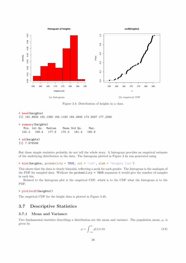
Figure 3.4: Distribution of heights in a class.
> head(heights)
[1] 181.8826 182.1380 184.1183 184.2845 173.2597 177.2280
> summary(heights)
Min. 1st Qu. Median Mean 3rd Qu. Max.
155.2 169.4 177.6 175.3 181.4 185.8
> sd(heights)
[1] 7.876596
But these simple statistics probably do not tell the whole story. A histogram provides an empirical estimateof the underlying distribution in the data. The histogram plotted in Figure 3.4a was generated using
> hist(heights, probability = TRUE, col = "red", xlab = "heights [cm]")
This shows that the data is clearly bimodal, reflecting a peak for each gender. The histogram is the analogue ofthe PDF for sampled data. Without the probability = TRUE argument it would give the number of samplesin each bin.
Related to the histogram plot is the empirical CDF, which is to the CDF what the histogram is to thePDF.
> plot(ecdf(heights))
The empirical CDF for the height data is plotted in Figure 3.4b.
3.7 Descriptive Statistics
3.7.1 Mean and Variance
Two fundamental statistics describing a distribution are the mean and variance. The population mean, µ, isgiven by
µ =
∫
∞
−∞
p(x)xdx (3.8)
26

while the population variance, σ2, is
σ2 =
∫
∞
−∞
p(x)(x − µ)2 dx, (3.9)
where σ is the standard deviation. In the discrete case these become
µ =∑
P (x)x (3.10)
andσ2 =
∑
P (x)(x − µ)2 dx (3.11)
where the summation is over the entire population.In practice it is generally not possible to evaluate either µ or σ2 since one has access to only a finite sample
from U . However, using the sample one is able to generate estimates of µ and σ2 using
x =1
N
∑
i
xi (3.12)
and
s2 =1
N − 1
∑
i
(xi − x)2 (3.13)
respectively, where
xN−→∞
µ and sN−→∞
σ.
Example: Measuring Length (revisited)
> sum(L) / length(L)
[1] 10.44
> sum((L - mean(L))**2) / (length(L) - 1)
[1] 0.007111111
The built in functions mean(), sd() and var() provide a more compact way to determine the sample mean,standard deviation and variance. Confirm that they give the same results!
3.7.2 Median and Quantiles
The median of a population is the value separating the “bigger”half of the population from the “smaller” half.In the case of a continuous distribution it is the x which satisfies
∫ x
−∞
p(ξ) dξ = 0.5.
In the case of a finite sample, the observations are sorted from smallest to largest and the value in the middleis the median. So, for example:
> x = runif(7)
> sort(x)
[1] 0.09554641 0.10842553 0.10897014 0.11887933 0.59698168 0.77841234 0.80596488
> median(x)
[1] 0.1188793
27

Quantiles are observations taken at regular intervals from the CDF. There are a few special varieties.Quartiles divide the CDF into four parts where the boundaries are defined by equating the CDF to 0, 0.25,0.5, 0.75 and 1.0.
> x = runif(13)
> sort(x)
[1] 0.02335965 0.05290677 0.27289543 0.28452226 0.32650875 0.50535291 0.58266771
[8] 0.58349524 0.58594230 0.58679542 0.63065159 0.87297827 0.90126201
> quantile(x)
0% 25% 50% 75% 100%
0.02335965 0.28452226 0.58266771 0.58679542 0.90126201
Referring to the CDF in Figure 3.3, the values on the y-axis define the quartile boundaries in the CDF.Mapping these across to the x-axis yields the required quartiles. Obviously P (x) = 0 maps to −∞ whileP (x) = 1 maps to ∞. The intermediate values at P (x) = 0.25, 0.5 and 0.75 map to -0.674, 0 and 0.674respectively. These are the quartiles of the Gaussian distribution.
Percentiles divide the CDF into 100 parts. So the first percentile occurs when the CDF is equal to 0.01.The median is the same as the fiftieth percentile. On the CDF plotted in Figure 3.3 these would be found bymarking off the y-axis at intervals of 0.01 from 0 to 1 and mapping these points across to the x-axis.
3.7.3 Expectation Value
The expectation value is a generalisation of the mean and corresponds to the mean value of a function, f(x),when the x are sampled from the corresponding distribution function:
E [f(x)] =
∫
∞
−∞
p(x)f(x) dx (3.14)
orE [f(x)] =
∑
P (x)f(x). (3.15)
The expectation operator is linear so that
E [f(x) + g(x)] = E [f(x)] + E [g(x)]
E [αf(x)] = αE [f(x)] .
3.8 Standard Distributions
A number of standard distributions exist. These are distributions which have a well defined analytical form.But apart from having a concise mathematical representation, many of them provide a good approximationto real world distributions.
3.8.1 Binomial
The binomial distribution is a discrete probability distribution that expresses the number of successes in asequence of independent experiments. The probability of k successes from N independent samples, where eachsample yields success with probability P is
P (k;N,P ) =
(
N
k
)
P k(1− P )N−k (3.16)
for k = 0, 1, 2, . . . , N and(
N
k
)
=N !
k!(N − k)!(3.17)
is the binomial coefficient.
28

Example: Binomial Distribution
The probability of throwing heads is 0.5. What is the likelihood of throwing heads 10 times out of 15?
> choose(15,10) * 0.5^10 * (1 - 0.5)^(15 - 10)
[1] 0.09164429
> dbinom(10, 15, 0.5)
[1] 0.09164429
The built in functions dbinom(), pbinom(), qbinom() and rbinom() all relate to the binomial distribution.
3.8.2 Poisson and Exponential
The Poisson distribution is a discrete probability distribution which describes the probability of a given numberof events (with a known average rate) occurring during a fixed period of time. The distribution need not beapplied exclusively in the temporal domain but is just as admissable to describing a distribution of events perunit length.
If the average number of events per unit time is λ, then the probability of k events in a unit interval is
P (k;λ) =λke−λ
k!. (3.18)
Obviously the mean is λ, while the standard deviation is√λ.
The radioactive decay of 267Sg has a half-life of 19ms. The decay constant is thus
> (lambda = log(2) / 19e-3)
[1] 36.48143
or an average rate of .3f s−1. Consider an experiment in which the number of decays in a 1 s interval is recorded.A series of such experiments is simulated using rpois(), which draws samples from a Poisson distribution.
> rpois(20, lambda)
[1] 37 35 27 25 28 38 34 40 34 42 43 30 24 27 26 43 36 38 41 36
These are the simulated number of decays in twenty 1 s intervals. For a very large number of experiments, thesample mean and standard deviation approach the theoretical values.
> decays <- rpois(1000, lambda)
> mean(decays)
[1] 36.543
> sd(decays)
[1] 5.970913
The histogram generated from these results is an approximation to the theoretical PDF, which is generatedusing dpois().
> hist(decays, probability = TRUE, xlab = "decays")
> lines(dpois(0:ceiling(max(decays)), lambda))
These are presented in Figure 3.5a. The corresponding empirical CDF, plotted in Figure 3.5b, also resemblesthe theoretical CDF, generated using ppois().
29

Histogram of decays
decays
Den
sity
20 30 40 50 60
0.00
0.01
0.02
0.03
0.04
0.05
0.06
(a) PDF
10 20 30 40 50 60
0.0
0.2
0.4
0.6
0.8
1.0
ecdf(decays)
decays
Fn(
x)(b) CDF
Figure 3.5: Radioactive decay process simulated using a Poisson distribution.
> plot(ecdf(decays), xlab = "decays")
> lines(ppois(0:ceiling(max(decays)), lambda))
Quantiles are generated using qpois().
> qpois(c(0, 0.25, 0.5, 0.75, 1), lambda)
[1] 0 32 36 40 Inf
So, 25% of the experiments observe 32 or fewer decays.If the number of events per unit time follows the Poisson distribution with mean λ, then the intervals
between events are described by an exponential distribution with mean 1/λ. The PDF of the exponentialdistribution is
p(x;λ) =
{
λe−λx for x ≥ 0
0 for x < 0.(3.19)
An analogous group of functions are defined for the exponential distribution. Consider another experimentin which the interval between successive decays is measured. To simulate this experiment, use rexp().
> intervals <- rexp(1000, lambda)
> head(intervals)
[1] 0.02537271 0.05280692 0.03657319 0.03905192 0.01292690 0.00127156
> mean(intervals)
[1] 0.0262431
This gives the intervals between 1000 decay events. The distribution of the intervals is plotted in Figure 3.6ausing
> hist(intervals, probability = TRUE, xlab = "seconds")
> t = seq(0, ceiling(max(intervals)), 0.025)
> lines(t, dexp(t, lambda))
30

Histogram of intervals
seconds
Den
sity
0.00 0.05 0.10 0.15
05
1015
2025
(a) PDF
0.00 0.05 0.10 0.15 0.20
0.0
0.2
0.4
0.6
0.8
1.0
ecdf(intervals)
seconds
Fn(
x)(b) CDF
Figure 3.6: Intervals in a radioactive decay process simulated using an Exponential distribution.
Figure 3.7: According to xkcd, there is still hope, even for those deep in the tails of the Gaussian distribution.
The corresponding empirical CDF, plotted in Figure 3.6b, conforms well to the theoretical CDF, generatedusing pexp().
> plot(ecdf(intervals), xlab = "seconds")
> lines(t, pexp(t, lambda), col = "red")
Quantiles are generated using qexp()
> qexp(seq(0, 1, 0.2), lambda)
[1] 0.000000000 0.006116634 0.014002346 0.025116634 0.044116634 Inf
So, 80% of the observed intervals are shorter than 0.044. Confirm that this is true from Figure 3.6b.
3.8.3 Gaussian
A Gaussian, or normal, distribution is a continuous probability distribution. A Gaussian with mean µ andvariance σ2 has a PDF of the form
p(x;µ, σ) =1√2πσ2
e−(x−µ)2/2σ2
. (3.20)
31

When the variance is zero the distribution becomes a delta function
p(x;µ, 0) = δ(x− µ). (3.21)
Drawing samples from a Gaussian distribution is done with rnorm(). To draw 5 samples from a Gaussiandistribution with a mean of 0 and standard deviation of 1 (these are actually the default values)
> rnorm(5, mean = 0, sd = 1)
[1] -0.32607191 0.37877737 0.54904574 1.12168604 0.06436539
> mean(rnorm(1000, 0, 1))
[1] 0.04633829
> sd(rnorm(1000, 0, 1))
[1] 1.008418
Quantiles are generated using qnorm()
> qnorm(c(0, 0.25, 0.5, 0.75, 1))
[1] -Inf -0.6744898 0.0000000 0.6744898 Inf
The PDF is evaluated with dnorm()
> dnorm(seq(-1, 1, 0.25))
[1] 0.2419707 0.3011374 0.3520653 0.3866681 0.3989423 0.3866681 0.3520653 0.3011374
[9] 0.2419707
While values of the CDF are generated by pnorm()
> pnorm(seq(-1, 1, 0.25))
[1] 0.1586553 0.2266274 0.3085375 0.4012937 0.5000000 0.5987063 0.6914625 0.7733726
[9] 0.8413447
If the distribution of x is described by (3.20), then the standardised variable
z =x− µ
σ(3.22)
has a Gaussian distribution with zero mean and unit variance,
p(z) =1√2π
e−z2/2. (3.23)
Example: Distribution of IMF components
From Figure 1.1 it might appear that the IMF Bz might be normally distributed. To test qualitatively whetherthis is feasible, a histogram is generated and compared to a fitted Gaussian distribution.
> hist(ACE$Bz, prob = TRUE, col = "grey", main = "", ylim = c(0, 0.25))
> lines(density(ACE$Bz, na.rm = TRUE), col = "red")
> x = seq(-15, 15, length = 200)
> lines(x, dnorm(x, mean(ACE$Bz, na.rm = TRUE), sd(ACE$Bz, na.rm = TRUE)))
32

ACE$Bz
Den
sity
−15 −10 −5 0 5 10 15
0.00
0.05
0.10
0.15
0.20
0.25
The red curve is a non-parametric estimate of the Bz density. Although the distribution appears superfi-cially to be normal, it is actually too sharply peaked.
> qqnorm(ACE$Bz)
> abline(0, 1)
> qqline(ACE$Bz, col = "red")
33

−4 −2 0 2 4
−15
−10
−5
05
10Normal Q−Q Plot
Theoretical Quantiles
Sam
ple
Qua
ntile
s
A quantile-quantile plot reinforces this conclusion. If the data were indeed normal the points in this plotwould lie along the dotted line. The quantile-quantile plot is formed from� quantiles from the empirical CDF derived from the data, and� the corresponding quantiles from the normal distribution.
The former are projected onto the y-axis while the latter are reflected on the x-axis. Obviously if the datawere sampled from a normal distribution then the points would fall on a line with unit slope passing throughthe origin. If the points stray significantly from this line then it is an indication that the data is not normallydistributed.
3.9 The Central Limit Theorem
Consider a sample (3.1) from a distribution with mean µ and standard deviation σ. As N →∞ the distributionof the sample mean, x, tends towards a normal distribution with mean µ and standard deviation σ/
√N . The
power of the Central Limit Theorem is that the distribution of the mean approaches a normal distributionregardless of the distribution of the underlying samples.
To clarify, the mean and variance of the sample are defined by (3.12) and (3.13). For clarity the samplevariance will be denoted here by s2x. The variance of the sample mean is then
s2x =s2xN
. (3.24)
Whereas s2x characterises the spread of the samples around the sample mean, s2x reflects the spread of themean. One might imagine taking a number of samples of size N from the population and calculating the mean
34

for each sample. The variance of the resulting set of mean values would be s2x. While the standard deviationof the sample remains more or less the same regardless of N , the standard deviation of the mean declines as1/√N : more samples lead to lower scatter.
Example: Variance of the Mean
Suppose that one drew samples of size 100, 1000 and 10000 from a Gaussian distribution with zero mean andσ = 2.
> g1 = rnorm(sd = 2, n = 100)
> g2 = rnorm(sd = 2, n = 1000)
> g3 = rnorm(sd = 2, n = 10000)
In each case the variance of the sample is roughly the same:
> c(var(g1), var(g2), var(g3))
[1] 3.854746 3.738802 3.938910
The variance of the mean declines with sample size:
> sd_mean <- function(x) {sd(x) / sqrt(length(x))}
> sd_mean(g1)
[1] 0.1963351
> sd_mean(g2)
[1] 0.06114574
> sd_mean(g3)
[1] 0.01984669
To illustrate this directly by generating multiple samples and finding the standard deviations of the resultingmeans:
> M <- 0
> for (i in 1:100) {M <- c(M, mean(rnorm(sd = 2, n = 100)))}
> sd(M)
[1] 0.1792964
> M <- 0
> for (i in 1:100) {M <- c(M, mean(rnorm(sd = 2, n = 1000)))}
> sd(M)
[1] 0.06486954
> M <- 0
> for (i in 1:100) {M <- c(M, mean(rnorm(sd = 2, n = 10000)))}
> sd(M)
[1] 0.01769911
35

ACCEPT
(a) two sided Ha
ACCEPT
(b) one sided Ha (left)
ACCEPT
(c) one sided Ha (right)
Figure 3.8: Possible configurations for alternative hypotheses, showing range in which the null hypothesis isaccepted.
Table 3.1: Types of error which might arise depending on the outcome of a test (positive or negative) forwhether a particular effect exists in the entire population (positive or negative).
testpopulation positive negativepositive Type IInegative Type I
3.10 Hypotheses
The null hypothesis (H0) is a conjecture which states that the effect of interest is not present in the population.The null hypothesis is assumed to be true until proven otherwise (subject to a particular degree of confidence).An alternative hypothesis (Ha) states that there is an effect. H0 and Ha necessarily represent disjoint regionsof the sample space: they cannot both be true at the same time! Alternative hypotheses may come in twopossible forms:� a one-sided hypothesis states that the effect is in only one direction (the result is greater than the null
value or the result is less than the null value)
H0 : µ ≤ µ0
Ha : µ > µ0
or
H0 : µ ≥ µ0
Ha : µ < µ0� a two-sided hypothesis states that the effect can be in either direction (the result is simply different fromthe null value)
H0 : µ = µ0
Ha : µ 6= µ0.
These two possibilities are illustrated in Figure 3.8.Of course, the application of the statistical decision process is not infallible and errors do occur. They are
classified as either
Type I Error (false positive) rejecting the null hypothesis when it is actually true;
Type II Error (false negative) failing to reject the null hypothesis when the alternative hypothesis is true.
These two types of error are illustrated in Table 3.1.
36

−3 −2 −1 0 1 2 3
0.0
0.1
0.2
0.3
0.4
x
p(x)
−3 −2 −1 0 1 2 3
0.0
0.1
0.2
0.3
0.4
x
p(x)
Figure 3.9: Calculation of one-sided p-values for a H0 given by (3.23).
3.11 Statistical (Un)certainty
Statistical certainty might seem like an oxymoron, and is probably better conceived of as statistical uncertainty.Once one has inferred a statistical estimate of some quantity, it is highly desirable to determine the quality ofthis estimate. An indication of the statistical uncertainty is commonly provided either by a confidence intervalor a p-value.
3.11.1 Statistical Significance
The significance level, α, is the threshold used for rejecting H0, and is effectively the probability of makinga Type I error. The significance level should be selected before analysing the data. The application of asignificance level proceeds as follows:
1. find the difference between the experimental results and H0;
2. assuming that H0 is true, determine the probability, p, of a difference that large or larger;
3. compare this probability to α and
p > α −→ accept H0,p < α −→ reject H0.
Typically, significance levels of α = 0.05 (5%) or α = 0.01 (1%) are used. For smaller α the data mustdiverge more substantially from H0 to be significant. Lower α therefore produces a more conservative result.
3.11.2 The p-value
The p-value associated with a statistic indicates the probability of making a Type I error (false positive). Thatis, it is the probability of a result at least as extreme as that obtained if the null hypothesis is actually true.Loosely speaking, the p-value is the probablity that a given result could have been obtained by chance.
If the sampled result differs from H0 then there is some evidence supporting Ha. The strength of this isdetermined by the p-value, the probability of obtaining this result were H0 indeed valid. A smaller p-valueindicates a more compelling result. If
p < α (3.25)
then the result is significant at the α level.
Example: The p-value
The distribution in Figure 3.9 has µ = 0 and σ = 1.
37

> 1 - pnorm(0.5)
[1] 0.3085375
> 1 - pnorm(2.5)
[1] 0.006209665
The probability of getting a result of 0.5 (or larger) is not terribly small. . . but the probability of getting 2.5(or larger) is rather small indeed. The significance of the latter result is thus a lot higher. At the α = 0.01significance level, H0 would be accepted in the former case, but it would certainly be rejected in the latter.This implies that a result which differs by that much from H0 could only be obtained in 1% of samples if H0
were true.
3.11.3 Confidence Intervals (Idealised)
A confidence interval is a range of possible values in which the sought after quantity might lie. Associatedwith the confidence interval is a confidence level which describes the likelihood that the true value lies withinthis range. The confidence level is related to the significance level: for a significance level of α, the confidencelevel is 1− α.
There is a direct relationship between the width of the confidence interval and the associated confidencelevel. The smaller the confidence level, the narrower the confidence interval and vice versa. This can besummarised as follows:� small α → large confidence level → broad confidence interval;� large α → small confidence level → narrow confidence interval.
So, α = 0.05 would correspond to a 95% confidence level and a relatively narrow confidence interval. Aα = 0.01 would correspond to a 99% confidence level and a broader confidence interval. To have a higher levelof confidence you must accept that the real value might be further from the estimated value. Therefore, inorder to have a smaller margin of error, one must compromise with a lower degree of confidence. A smallerconfidence interval may be obtained for a given confidence level by increasing N .
Two-Sided Ha
If the quantity is assumed to have a normal distribution then a confidence interval with associated probability1− α is determined by finding the central area under (3.23) leaving α/2 on either side. Expressed in terms ofstandardised variables, we seek an interval extending from −z∗ to z∗ such that
P (−z∗ ≤ Z ≤ z∗) = 1− α
which is the same asP (Z ≤ z∗) = 1− α
2.
The required z∗ is found by inverting the CDF. That is, one seeks the upper critical value, z∗, such that
∫ z∗
−∞
p(x) dx =α
2+ 1− α = 1− α
2. (3.26)
The corresponding confidence interval extends z∗ standard deviations on either side of the experimental result.With probability α/2 the true value may lie to the left of this interval, and with probability α/2 the true valuemay lie to the right of this interval.
For example, with α = 0.05, we find
> alpha = 0.05
> qnorm(1 - alpha / 2)
[1] 1.959964
38
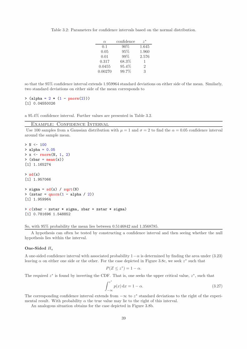
Table 3.2: Parameters for confidence intervals based on the normal distribution.
α confidence z∗
0.1 90% 1.6450.05 95% 1.9600.01 99% 2.5760.317 68.3% 10.0455 95.4% 20.00270 99.7% 3
so that the 95% confidence interval extends 1.959964 standard deviations on either side of the mean. Similarly,two standard deviations on either side of the mean corresponds to
> (alpha = 2 * (1 - pnorm(2)))
[1] 0.04550026
a 95.4% confidence interval. Further values are presented in Table 3.2.
Example: Confidence IntervalUse 100 samples from a Gaussian distribution with µ = 1 and σ = 2 to find the α = 0.05 confidence intervalaround the sample mean.
> N <- 100
> alpha = 0.05
> x <- rnorm(N, 1, 2)
> (xbar = mean(x))
[1] 1.165274
> sd(x)
[1] 1.957066
> sigma = sd(x) / sqrt(N)
> (zstar = qnorm(1 - alpha / 2))
[1] 1.959964
> c(xbar - zstar * sigma, xbar + zstar * sigma)
[1] 0.781696 1.548852
So, with 95% probability the mean lies between 0.5146842 and 1.3568785.
A hypothesis can often be tested by constructing a confidence interval and then seeing whether the nullhypothesis lies within the interval.
One-Sided Ha
A one-sided confidence interval with associated probability 1−α is determined by finding the area under (3.23)leaving α on either one side or the other. For the case depicted in Figure 3.8c, we seek z∗ such that
P (Z ≤ z∗) = 1− α.
The required z∗ is found by inverting the CDF. That is, one seeks the upper critical value, z∗, such that∫ z∗
−∞
p(x) dx = 1− α. (3.27)
The corresponding confidence interval extends from −∞ to z∗ standard deviations to the right of the experi-mental result. With probability α the true value may lie to the right of this interval.
An analogous situation obtains for the case depicted in Figure 3.8b.
39

3.11.4 Confidence Intervals (Realistic)
The foregoing discussion only really applies as N → ∞. The Student’s t distribution assumes that the dataresembles a normal distribution but takes into account the finite sample size by specifying the number ofdegrees of freedom, which is N − 1 assuming that the mean has been estimated from the data.
> alpha = 0.05
> qnorm(1 - alpha / 2)
[1] 1.959964
> N = 10
> qt(1 - alpha / 2, N - 1)
[1] 2.262157
So that for a small sample there is a clear difference. As the number of degrees of freedom increases, theStudent’s t distribution converges to a normal distribution.
> qt(1 - alpha / 2, 10^c(1, 2, 3, 4, 5, 6))
[1] 2.228139 1.983972 1.962339 1.960201 1.959988 1.959966
3.12 Statistical Tests
3.12.1 Test for Population Mean (Known Standard Deviation)
Suppose that one wanted to test the hypothesis that the population mean was equal to µ0. The null hypothesiswould be
H0: µ = µ0.
The test is applied to the standardised variable (3.22) as
z =x− µ0
σ/√N
, (3.28)
which has a normal distribution when H0 is true. The appropriate p-value for each of the three possiblealternative hypotheses is found from
Ha: µ > µ0 P = P (Z ≥ z∗) (refer to Figure 3.8c)
Ha: µ < µ0 P = P (Z ≤ z∗) (refer to Figure 3.8b)
Ha: µ 6= µ0 P = P (Z ≥ |z∗|) (refer to Figure 3.8a).
3.12.2 Test for Population Mean (Unknown Standard Deviation)
In practice neither the standard deviation, σ, nor the standard deviation of the mean, σ/√N , are known.
When σ is not known, the sample estimate, s, is used and the standard deviation of the mean is estimated ass/√N . The z statistic is then replaced by the t statistic,
t =x− µ0
s/√N
. (3.29)
However, unless the sample size is relatively large, the distribution of t is not precisely normal. It is insteaddescribed by a t distribution with N − 1 degrees of freedom. The shape of the t distribution changes withthe number of samples (or, equivalently, the degrees of freedom), but becomes the Gaussian distribution asN →∞.
The appropriate confidence interval is
x± t∗s√N
40

where t∗ is the upper critical value of the appropriate t distribution. Similarly, the p-values for the alternativehypotheses are found from
Ha: µ > µ0 P = P (T ≥ t∗)
Ha: µ < µ0 P = P (T ≤ t∗)
Ha: µ 6= µ0 P = P (T ≥ |t∗|).
For example, to test whether the average value of the speed of light calculated from the experiments ofMichaelson and Morley agrees with the currently accepted value of 2.99792458× 10⁵ km/s:
> mean(morley$Speed)
[1] 852.4
> sd(morley$Speed)
[1] 79.01055
> t.test(morley$Speed, mu = 2.99792458e5 - 2.99e5)
One Sample t-test
data: morley$Speed
t = 7.5866, df = 99, p-value = 1.824e-11
alternative hypothesis: true mean is not equal to 792.458
95 percent confidence interval:
836.7226 868.0774
sample estimates:
mean of x
852.4
This indicates that the speed originally derived by Michaelson and Morley differs significantly at the 95% level(α = 0.05)!
3.12.3 Comparing Two Means
Suppose one wanted to know whether two distributions had the same mean value. This might be of interest ifone were to make measurements of a given quantity before and after a specific event took place. For example,the quantity of sulphur dioxide in the atmosphere before and after a volcanic eruption. If the two measurementsdiffer then it is important to assess the statistical significance of the difference.
Consider two populations, which will be denoted A and B. The population mean and standard deviationfor population A are denoted µA and σA, while the corresponding parameters from NA samples are xA andsA. Analogous symbols apply to population B. The appropriate t statistic is
t =(xA − xB)− (µA − µB)√
s2A/NA + s2B/NB
. (3.30)
The resulting confidence interval for µA − µB is
(xA − xB)± t∗√
s2A/NA + s2B/NB
where t∗ is the upper critical value of the t distribution with degrees of freedom equal to the smaller of NA− 1and NB − 1.
For example, to test whether the average speed of light differed between the first two sets of Michaelsonand Morley experiments:
> t.test(morley$Speed[morley$Expt == 1], morley$Speed[morley$Expt == 2])
Welch Two Sample t-test
data: morley$Speed[morley$Expt == 1] and morley$Speed[morley$Expt == 2]
41

t = 1.9516, df = 30.576, p-value = 0.0602
alternative hypothesis: true difference in means is not equal to 0
95 percent confidence interval:
-2.419111 108.419111
sample estimates:
mean of x mean of y
909 856
Therefore the values do not differ significantly at the 95% level.
3.13 Covariance and Correlation
Inspection of Figure 1.1 suggests that periods of high solar wind number density have low flow speed, andvice versa. In contrast, periods of high solar wind speed correspond to intervals of high plasma temperatureand vice versa. There seem to be qualitative relationships between these variables. The relationships may bequantified by means of covariance and correlation.
Covariance is a measure of how much the variation in one variable is related to the variation in another.The covariance is defined as
cov(x, y) = E [(x− x)(y − y)] . (3.31)
The sign of the covariance is determined by the joint signs of the residuals for x and y:
x− x y − y+ + +− − ++ − −− + −
Expanding (3.31)
cov(x, y) = E [xy]− xE [y]− E [x] y + xy
= E [xy]− xy.
When x and y are independent, E [xy] = xy and cov(x, y) = 0.
> cov(sin(1:10), 2*sin(1:10))
[1] 1.067175
> cov(sin(1:10), cos(1:10))
[1] 0.05814238
> cov(ACE$N, ACE$v)
[1] NA
> cov(ACE$N, ACE$v, use = "complete.obs")
[1] -159.1574
> ace <- ACE[, c("N", "v", "T")]
> ace <- ace[!rowSums(is.na(ace)),]
> cov(ace)
N v T
N 16.82050 -159.1574 -59268.05
v -159.15736 8243.8624 4069541.60
T -59268.05496 4069541.5957 3990479164.17
42

The covariance of two variables is simply a number. The covariance between more than two variables isgenerally presented as a (symmetric) covariance matrix.
The utility of the covariance is limited by the fact that the results are not normalised: one can’t directlycompare the magnitude of cov(x, y) with cov(x, z). This difficulty is addressed with the correlation coefficient.
The Pearson’s product moment correlation coefficient is defined as
ρ =E [(x− x)(y − y)]
sxsy(3.32)
which is the ratio of the covariance to the product of the respective standard deviations. The expected valueof the correlation for the entire population is denoted ρ, while the sample correlation is generally indicated byr. The square of r gives the fraction of variance which is common between the two variables. It is sometimescalled the coefficient of determination. The value of r is confined to the range [−1, 1], where r ∼ −1 indicatesa strong anti-correlation (data are in antiphase) while r ∼ 1 shows a clear positive correlation (data are inphase).
The correlation coefficient depends on the number of independent samples. If successive samples arecorrelated then the correlation coefficient needs to be adjusted by using an effective sample size [Meko, Chapters9 and 10].
The first step in understanding correlation is to standardise the variation in the data:
z ← x− x
s.
This standard score or standard anomaly is a dimensionless quantity which has a mean of zero, unit standarddeviation, and is commonly denoted by z. Standardisation can be accomplished using scale().
> head(ace)
N v T
1 3.5 284 24501
2 3.9 280 27812
3 3.7 280 24882
4 3.7 282 23331
5 3.7 282 21154
6 3.5 281 20568
> apply(ace, 2, mean)
N v T
5.512821 403.782952 74015.260132
> apply(ace, 2, sd)
N v T
4.10128 90.79572 63170.23954
> d <- scale(ace)
> head(d)
N v T
1 -0.4907787 -1.319258 -0.7838226
2 -0.3932482 -1.363313 -0.7314087
3 -0.4420134 -1.363313 -0.7777913
4 -0.4420134 -1.341285 -0.8023440
5 -0.4420134 -1.341285 -0.8368064
6 -0.4907787 -1.352299 -0.8460829
> apply(d, 2, mean)
N v T
7.507557e-17 1.805869e-16 -4.129936e-17
43
> apply(d, 2, sd)
N v T
1 1 1
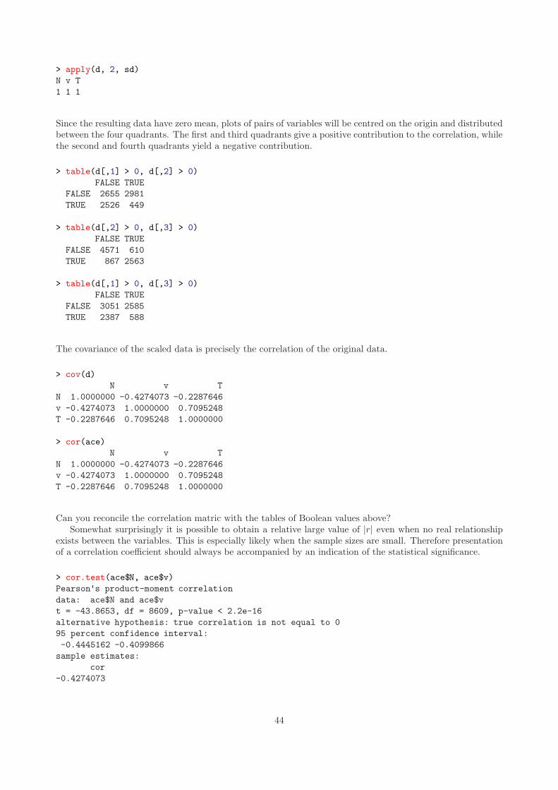
Since the resulting data have zero mean, plots of pairs of variables will be centred on the origin and distributedbetween the four quadrants. The first and third quadrants give a positive contribution to the correlation, whilethe second and fourth quadrants yield a negative contribution.
> table(d[,1] > 0, d[,2] > 0)
FALSE TRUE
FALSE 2655 2981
TRUE 2526 449
> table(d[,2] > 0, d[,3] > 0)
FALSE TRUE
FALSE 4571 610
TRUE 867 2563
> table(d[,1] > 0, d[,3] > 0)
FALSE TRUE
FALSE 3051 2585
TRUE 2387 588
The covariance of the scaled data is precisely the correlation of the original data.
> cov(d)
N v T
N 1.0000000 -0.4274073 -0.2287646
v -0.4274073 1.0000000 0.7095248
T -0.2287646 0.7095248 1.0000000
> cor(ace)
N v T
N 1.0000000 -0.4274073 -0.2287646
v -0.4274073 1.0000000 0.7095248
T -0.2287646 0.7095248 1.0000000
Can you reconcile the correlation matric with the tables of Boolean values above?Somewhat surprisingly it is possible to obtain a relative large value of |r| even when no real relationship
exists between the variables. This is especially likely when the sample sizes are small. Therefore presentationof a correlation coefficient should always be accompanied by an indication of the statistical significance.
> cor.test(ace$N, ace$v)
Pearson's product-moment correlation
data: ace$N and ace$v
t = -43.8653, df = 8609, p-value < 2.2e-16
alternative hypothesis: true correlation is not equal to 0
95 percent confidence interval:
-0.4445162 -0.4099866
sample estimates:
cor
-0.4274073
44
So that the correlation between plasma density and speed appears to be significant. On the other hand thefinite correlation between two short random sequences is not significant at all!
> cor.test(runif(10), runif(10))
Pearson's product-moment correlation
data: runif(10) and runif(10)
t = -1.1611, df = 8, p-value = 0.2791
alternative hypothesis: true correlation is not equal to 0
95 percent confidence interval:
-0.8146057 0.3283915
sample estimates:
cor
-0.3797543
3.13.1 Requirements and Assum,ptions
In order to calculate the correlation between two data sequences it is necessary that each possess the samenumber of terms. This is non-negotiable. Furthermore, the correlation also assumes that the sequences areordered in such a way that each observation in one sequence is associated with the corresponding observationin the other sequence: either they were made at the same time or the same place. A generalisation of thecorrelation considers shifting the one sequence with respect to the other before generating the correlation. . .but more of that later.
3.13.2 Correlation and Causality
If two variables have a strong correlation does this imply a causal relationship between them? Certainly not.They may indeed be causally related but correlation is not enough to establish such a relationship.
Figure 3.10: Even xkcd acknowledges that a finite correlation does not necessarily imply a causal relationship.
Example: Mobile Phone Masts and Birth Rate
A study was carried out to relate the number of mobile phone masts in each county across the UnitedKingdom to the live birth data for the same counties. The resulting correlation coefficient was found to be0.981 (p≪ 0.01), which is a rather compelling result. Does this imply that mobile phone masts are implicatedin increased fertility or more frequency sexual encounters? No! Not at all. Both the number of masts and thenumber of births are linked to a third parameter: the population. As the population increases, both of theother variables increase as well.
45

3.14 Exercises
Exercise 3.1. Draw a Venn diagram to convince yourself that (3.4) is true.
Exercise 3.2. Plot a histogram and an empirical CDF for the GSTA data. Is the relationship between thesetwo plots clear?
Exercise 3.3. Calculate the mean and standard deviation of the ACE solar wind speed
(i) using the builtin functions, mean() and sd(), and
(ii) by writing your own functions, MEAN() and SD().
Exercise 3.4. Use the binomial distribution to determine the probability of drawing 10 odd numbers and 20even numbers when samples are taken from {1, 2, . . . , 100}. Next find the probability of drawing a sample ofsize 20 from the same population, in which half the sample data are divisible by 5.
Exercise 3.5. Calculate numerically the average number of successes from a binomial experiment in whichsamples of size 20 are drawn and the probability of success for a single event is 0.25?
Exercise 3.6. Generate a series of uniformly distributed random numbers between 0 and 100. Then
(i) calculate the mean, x;
(ii) calculate the standard deviation;
(iii) calculate the standard deviation of the mean;
(iv) does x differ from µ significantly at the α = 0.05 level?
(v) find the α = 0.01 confidence interval for x.
Exercise 3.7. Generate 1000 samples from an exponential distribution with λ = 1Hz then
(i) plot a histogram of the sampled delays;
(ii) accumulate the delays to yield a vector with the actual times of the sampled events;
(iii) generate an appropriate factor and count the number of events in each 1 s interval;
(iv) calculate the mean number of events per 1 s interval. Does it agree with the value of λ?
Exercise 3.8. Generate 1000 samples from a normal distribution with zero mean and unit variance. Plot ahistogram of the data and overlay a non-parameteric estimate of the density function. Using a quantile-quantileplot verify that the distribution of the data is approximately normal.
Exercise 3.9. Generate 1000 samples from a normal distribution with zero mean and unit variance. Whatpercentage of the sample lies within one standard deviation of the mean? Does this agree with the informationin Table 3.2?
Exercise 3.10. Describe the two possible errors which might arise from a pregnancy test. Which has the moresignificant consequences?
Exercise 3.11. Using the ACE data from
(i) define columns for day number and hour (use string manipulation functions);
(ii) plot the three components of B as a function of time (maybe use fractional day number as the abscissa?),overlaying each onto the same set of axes;
(iii) add a column for the angle, θ, between the projection of B onto the ecliptic plane and the Sun-Earthline;
(iv) plot the distribution of θ;
(v) what is the average value of θ and does it differ significantly from the expected value of 45◦ at theα = 0.05 level?
Exercise 3.12. Using the ACE data
46

(i) define a factor for day number;
(ii) calculate the average |B| for each day;
(iii) on which day is the average |B| greatest?
(iv) plot separate histograms for the distribution of |B| during October and November;
(v) comment on the histograms.
Exercise 3.13. Using the ACE data
(i) calculate the average solar wind speed for 1 November 2003;
(ii) find the corresponding α = 0.05 confidence interval;
(iii) calculate the average solar wind speed for the entire data set;
(iv) does the value for 1 November 2003 differ significantly from that for the entire data set at the α = 0.01significance level? What is the p-value? What does this mean?
Exercise 3.14. Using the ACE data
(i) identify one pair of solar wind variables that are positively correlated (r ≥ 0.5) and another pair whichare negatively correlated (r ≤ −0.5);
(ii) are these correlations significant at the α = 0.01 level?
(iii) find the α = 0.01 confidence intervals for r in each case.
Exercise 3.15. Generate a correlation matrix for the three components of the ACE magnetic field. Which pairof components is significantly correlated at the 99% level?
47
Chapter 4
Time Series
In statistics, signal processing, mathematical finance and a number of other disciplines, a time series is asequence of data points, typically measured at uniform time intervals. Such a times series might take the form
{xi|i = 1, . . .N} (4.1)
where xi is a measurement of x at time ti. The data plotted in Figure 1.1 are examples of time series. In thecase of uniform sampling
ti = t0 + i∆t (4.2)
where ∆t is the sampling interval. Although time series generally consist of observations made at differentinstants in time, the same techniques may be applied to data which consists of a set of measurements madeat different locations.
The observations in a time series can be treated as if they are independent, where each xi does not dependon any of the preceding observations. However, this is not a valid assumption since one of the intrinsiccharacteristics of a non-trivial time series is a certain degree of correlation between successive samples. Inmany situations values tend to cluster, with a high value following high values and a low value followinglow values. The order of the observations is therefore important and statistical techniques which requireindependent observations are thus not applicable.
Analyses of time series may be performed in either the time domain or the frequency domain. . . or both.Time domain techniques will be considered first.
In R a time series object is created with the generic ts() function. There are three important argumentsto ts(): data, start and frequency. They need not all be specified. To create an empty time series
> ts()
Time Series:
Start = 1
End = 1
Frequency = 1
[1] NA
But that is not much use, so the first thing to do is provide some data
> (t = ts(rnorm(7)))
Time Series:
Start = 1
End = 7
Frequency = 1
[1] -2.7747448 0.1668216 -0.7922744 0.2770606 -0.3146484 0.6834993 -1.6284054
> start(t)
[1] 1 1
48
> end(t)
[1] 7 1
Here the start and end of the object reflect the length of the time series, but their values are arbitrary. Supposethat the data correspond to annual values starting in 1994 then
> ts(rnorm(7), start = 1994)
Time Series:
Start = 1994
End = 2000
Frequency = 1
[1] -1.43130208 1.57383485 -0.84552883 0.29473650 0.41751362 0.03916673 0.32857905
If, instead, the values were quarterly and the time series started in the second quarter of 1994 then
> (t = ts(rnorm(7), start = c(1994, 2), frequency = 4))
Qtr1 Qtr2 Qtr3 Qtr4
1994 0.6915952 -0.3972122 1.8279316
1995 0.8919680 -2.5260557 0.4984289 -1.8985213
> frequency(t)
[1] 4
In this form the two element vector passed to the start parameter gives the starting time (in the natural timeunit, years) as the first element and the number of samples into the time unit as the second element. Thenumber of divisions within a time unit is specified by the frequency parameter. The corresponding times are
> time(t)
Qtr1 Qtr2 Qtr3 Qtr4
1994 1994.25 1994.50 1994.75
1995 1995.00 1995.25 1995.50 1995.75
This indicates that the values are assigned to the start of the intervals. Monthly data are created in a similarway
> (t = ts(rnorm(24), start = c(1994, 4), frequency = 12))
Jan Feb Mar Apr May Jun Jul
1994 0.72444801 1.07997614 2.16912761 0.94941390
1995 1.01036638 0.21019861 -2.53568214 -1.31241876 -0.48521425 -0.13456548 0.74980827
1996 -0.85359405 0.32690506 -0.15952162
Aug Sep Oct Nov Dec
1994 -0.06921355 -0.50253075 -0.87326327 2.11580918 1.40110712
1995 -0.07385563 -1.28290422 0.13008833 0.53774626 -0.19474606
1996
A portion of a time series can be extracted using window().
> window(t, start = c(1995, 6))
Jan Feb Mar Apr May Jun Jul Aug
1995 -0.13456548 0.74980827 -0.07385563
49
1996 -0.85359405 0.32690506 -0.15952162
Sep Oct Nov Dec
1995 -1.28290422 0.13008833 0.53774626 -0.19474606
1996
> window(t, start = c(1995, 6), end = c(1996, 1))
Jan Feb Mar Apr May Jun Jul Aug Sep
Oct
1995 -0.13456548 0.74980827 -0.07385563 -1.28290422
0.13008833
1996 -0.85359405
Nov Dec
1995 0.53774626 -0.19474606
1996
It can also be used to resample the data at a different frequency.
> window(t, frequency = 4)
Qtr1 Qtr2 Qtr3 Qtr4
1994 0.7244480 0.9494139 -0.8732633
1995 1.0103664 -1.3124188 0.7498083 0.1300883
1996 -0.8535940
Alternative functions for creating time series objects are discussed by Wurtz et al. [2009].Although ts() appears to cater solely for the year as a natural time unit, this is really not the case.
Suppose that a time series is sampled at one minute intervals and that sampling starts at 09:15 then one mightrepresent it using the minute as the natural time unit:
> ts(rnorm(7), start = 15)
Time Series:
Start = 15
End = 21
Frequency = 1
[1] 0.10399539 0.67648059 -1.09249729 -2.07588552 -0.27292475 -0.03989047 0.11151999
Or, alternatively, with the hour as natural time unit
> ts(rnorm(7), start = c(9, 15), frequency = 60)
Time Series:
Start = c(9, 15)
End = c(9, 21)
Frequency = 60
[1] 0.2351923 -0.8903969 -0.1606566 1.1412194 -0.8564781 0.8434788 -1.5768676
Now, moving from synthetic data to something more real. The GSTA data is converted into a time seriesobject as follows:
> head(GSTA)
year month deltaT fyear
1 1880 1 -0.0360 1880.000
2 1880 2 -0.1819 1880.083
50

3 1880 3 -0.1947 1880.167
4 1880 4 -0.0886 1880.250
5 1880 5 -0.1114 1880.333
6 1880 6 -0.1533 1880.417
> deltaT = ts(GSTA$deltaT, start = c(1880, 1), end = c(2010, 12), frequency = 12)
> window(deltaT, start = c(2006,1))
Jan Feb Mar Apr May Jun Jul Aug Sep Oct Nov Dec
2006 0.4054 0.5436 0.5222 0.4601 0.4816 0.6136 0.5858 0.5730 0.6026 0.6407 0.5953 0.7241
2007 0.8187 0.5928 0.6019 0.6766 0.5131 0.4785 0.4762 0.4846 0.5475 0.5156 0.4723 0.4328
2008 0.2227 0.3527 0.7110 0.4354 0.4368 0.4880 0.5123 0.4898 0.4620 0.6113 0.6031 0.4852
2009 0.5011 0.4891 0.5105 0.6010 0.5299 0.6051 0.5671 0.6266 0.6244 0.5653 0.5859 0.5015
2010 0.6106 0.6333 0.7755 0.7290 0.6900 0.6569 0.6409 0.5641 0.4846 0.5269 0.6998 0.3779
> window(deltaT, start = c(2006,1), frequency = 4)
Qtr1 Qtr2 Qtr3 Qtr4
2006 0.4054 0.4601 0.5858 0.6407
2007 0.8187 0.6766 0.4762 0.5156
2008 0.2227 0.4354 0.5123 0.6113
2009 0.5011 0.6010 0.5671 0.5653
2010 0.6106 0.7290 0.6409 0.5269
Here the year number is used as the natural unit for the time series and, since the data is presented as monthlyvalues, the sampling frequency is 12. The resulting object is plotted in Figure 4.1 using
> plot(deltaT, ylab = expression(paste(Delta, "T")))
The ACE data has 24 samples per day and extends over a full year. It is still possible to use ts() to createthe corresponding time series.
> Dst = ts(ACE$Dst, frequency = 24)
Another possibility is to use the zoo package.
> library(zoo)
> Dst = zoo(ACE$Dst, as.POSIXct(ACE$datetime, format = "%d-%m-%Y %H:%M:%S", tz = "UTC"))
4.1 Trend and Seasonality
A time series generally consists of a systematic pattern and random noise (which might make the patterndifficult to identify). The systematic pattern is most often either a trend or a seasonal variation, or both. Thetrend may be either a linear or non-linear change over time which does not repeat itself. A trend will resultin a change in the short-term mean. An example is the apparent increase in temperature reflected by recentclimatic data. In assessing a trend it is important to take into account the time scales of the data. Whatappears to be a trend over the short term might in fact form part of a longer term cycle. A seasonal cycle isa regular cyclic change, possibly with a changing amplitude. The cycle need not necessarily correspond to themeteorological concept of seasons but can be any pattern that repeats itself at regular intervals. Examples arelocal temperature which can exhibit diurnal, seasonal, annual, and sometimes semi-annual, variations; whileelectrical power consumption might have a hebdomadal (weekly) cycle.
The first step in a time series analysis is often a decomposition of the time series into a trend, a seasonalcomponent and the residual variations. An example of data which would benefit from this procedure is theAirPassengers data set plotted in Figure 4.2, from which it is apparent that there is a gradual increase inthe number of international airline passengers from year to year (the trend) and an annual peak during theNorthern Hemisphere summer (the seasonal cycle).
51
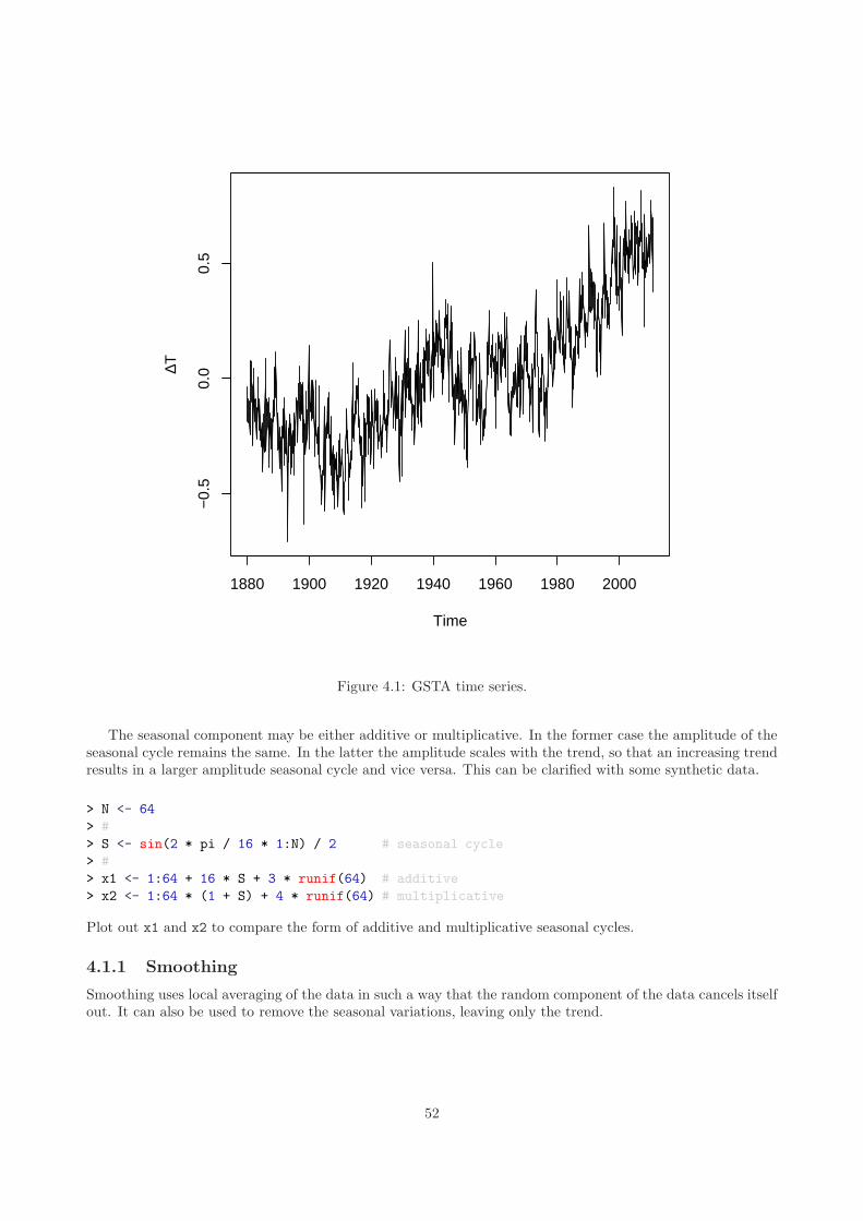
Time
∆T
1880 1900 1920 1940 1960 1980 2000
−0.
50.
00.
5
Figure 4.1: GSTA time series.
The seasonal component may be either additive or multiplicative. In the former case the amplitude of theseasonal cycle remains the same. In the latter the amplitude scales with the trend, so that an increasing trendresults in a larger amplitude seasonal cycle and vice versa. This can be clarified with some synthetic data.
> N <- 64
> #
> S <- sin(2 * pi / 16 * 1:N) / 2 # seasonal cycle
> #
> x1 <- 1:64 + 16 * S + 3 * runif(64) # additive
> x2 <- 1:64 * (1 + S) + 4 * runif(64) # multiplicative
Plot out x1 and x2 to compare the form of additive and multiplicative seasonal cycles.
4.1.1 Smoothing
Smoothing uses local averaging of the data in such a way that the random component of the data cancels itselfout. It can also be used to remove the seasonal variations, leaving only the trend.
52
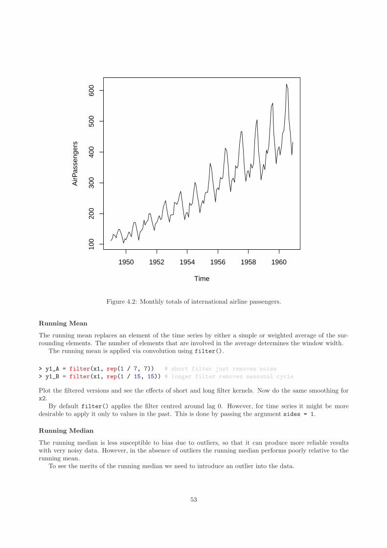
Time
AirP
asse
nger
s
1950 1952 1954 1956 1958 1960
100
200
300
400
500
600
Figure 4.2: Monthly totals of international airline passengers.
Running Mean
The running mean replaces an element of the time series by either a simple or weighted average of the sur-rounding elements. The number of elements that are involved in the average determines the window width.
The running mean is applied via convolution using filter().
> y1_A = filter(x1, rep(1 / 7, 7)) # short filter just removes noise
> y1_B = filter(x1, rep(1 / 15, 15)) # longer filter removes seasonal cycle
Plot the filtered versions and see the effects of short and long filter kernels. Now do the same smoothing forx2.
By default filter() applies the filter centred around lag 0. However, for time series it might be moredesirable to apply it only to values in the past. This is done by passing the argument sides = 1.
Running Median
The running median is less susceptible to bias due to outliers, so that it can produce more reliable resultswith very noisy data. However, in the absence of outliers the running median performs poorly relative to therunning mean.
To see the merits of the running median we need to introduce an outlier into the data.
53

Time
suns
pots
1800 1820 1840 1860 1880 1900
050
100
150
200
Figure 4.3: Smoothing of sunspot data.
> x2[20] = 300
> y2_A = filter(x2, rep(1 / 7, 7)) # the outlier distorts the data after running mean
> y2_B = runmed(x2, 7) # but the running median does much better!
A comparison of the effect of running mean and running median on the sunspot data is presented inFigure 4.3.
> k = 25
> spot = window(sunspots, start = 1800, end = 1900)
> spot = ts.union(spot, filter(spot, rep(1 / k, k)), runmed(spot, k))
> plot(spot[,1], ylab = "sunspots")
> lines(spot[,2], col = "red", lwd = 2)
> lines(spot[,3], col = "blue", lwd = 2, lty = "dashed")
4.1.2 Decomposition
Decomposition is the separation of a time series into trend, seasonal cycle and residuals. R has two functionsfor effecting a decomposition: decompose() and stl(). The latter uses a non-parametric technique to obtainan estimate of the trend. The first argument to either decompose() or stl() is a time series object. The
54
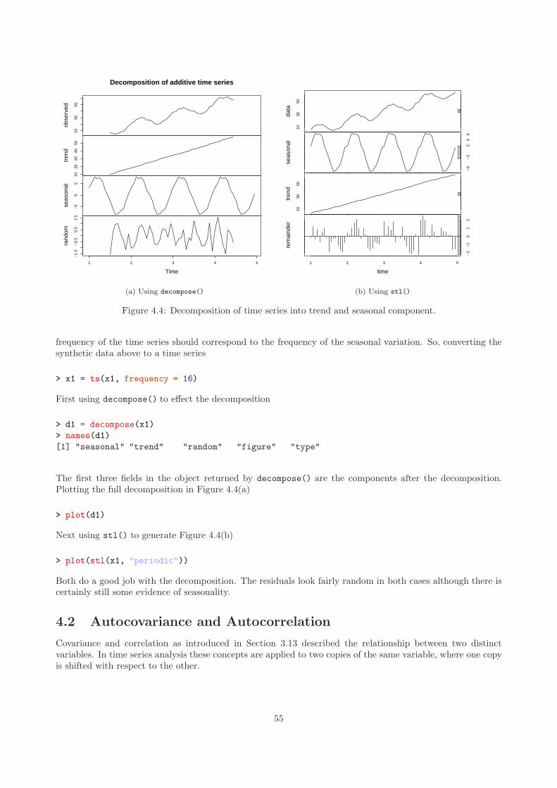
1030
50
obse
rved
1020
3040
50
tren
d
−5
05
seas
onal
−1.
5−
0.5
0.5
1.5
1 2 3 4 5
rand
om
Time
Decomposition of additive time series
(a) Using decompose()10
3050
data
−6
−2
24
6
seas
onal
1030
50
tren
d
−2
−1
01
2
1 2 3 4 5
rem
aind
er
time
(b) Using stl()
Figure 4.4: Decomposition of time series into trend and seasonal component.
frequency of the time series should correspond to the frequency of the seasonal variation. So, converting thesynthetic data above to a time series
> x1 = ts(x1, frequency = 16)
First using decompose() to effect the decomposition
> d1 = decompose(x1)
> names(d1)
[1] "seasonal" "trend" "random" "figure" "type"
The first three fields in the object returned by decompose() are the components after the decomposition.Plotting the full decomposition in Figure 4.4(a)
> plot(d1)
Next using stl() to generate Figure 4.4(b)
> plot(stl(x1, "periodic"))
Both do a good job with the decomposition. The residuals look fairly random in both cases although there iscertainly still some evidence of seasonality.
4.2 Autocovariance and Autocorrelation
Covariance and correlation as introduced in Section 3.13 described the relationship between two distinctvariables. In time series analysis these concepts are applied to two copies of the same variable, where one copyis shifted with respect to the other.
55
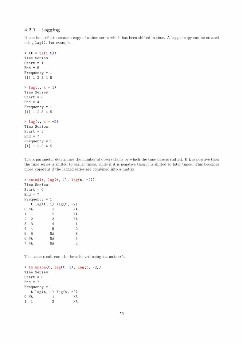
4.2.1 Lagging
It can be useful to create a copy of a time series which has been shifted in time. A lagged copy can be createdusing lag(). For example,
> (t = ts(1:5))
Time Series:
Start = 1
End = 5
Frequency = 1
[1] 1 2 3 4 5
> lag(t, k = 1)
Time Series:
Start = 0
End = 4
Frequency = 1
[1] 1 2 3 4 5
> lag(t, k = -2)
Time Series:
Start = 3
End = 7
Frequency = 1
[1] 1 2 3 4 5
The k parameter determines the number of observations by which the time base is shifted. If k is positive thenthe time series is shifted to earlier times, while if it is negative then it is shifted to later times. This becomesmore apparent if the lagged series are combined into a matrix
> cbind(t, lag(t, 1), lag(t, -2))
Time Series:
Start = 0
End = 7
Frequency = 1
t lag(t, 1) lag(t, -2)
0 NA 1 NA
1 1 2 NA
2 2 3 NA
3 3 4 1
4 4 5 2
5 5 NA 3
6 NA NA 4
7 NA NA 5
The same result can also be achieved using ts.union().
> ts.union(t, lag(t, 1), lag(t, -2))
Time Series:
Start = 0
End = 7
Frequency = 1
t lag(t, 1) lag(t, -2)
0 NA 1 NA
1 1 2 NA
56

2 2 3 NA
3 3 4 1
4 4 5 2
5 5 NA 3
6 NA NA 4
7 NA NA 5
The result is a multivariate time series which can be indexed like a matrix or data frame. To extract theportion of this matrix for which all time series have valid data use ts.intersect().
> ts.intersect(t, lag(t, 1), lag(t, -2))
Time Series:
Start = 3
End = 4
Frequency = 1
t lag(t, 1) lag(t, -2)
3 3 4 1
4 4 5 2
As mentioned previously, time series data are often characterised by a relatively high level of redundancy be-tween successive terms: high values are clustered together, low values are clustered together. This is illustratedin Figure 4.5 where pairs (xi, xi+1) from the GSTA data are plotted using
> plot(deltaT, lag(deltaT), xlab = expression(x[i]), ylab = expression(x[i+1]))
4.2.2 Autocovariance
Autocovariance is analogous to covariance. However, rather than calculating the covariance between xi and yi,the autocovariance is the covariance of xi with another instance of itself, xi+k, that has been shifted k samplesrelative to xi.
The autocovariance at lag k is defined as
γk = cov(xi, xi+k). (4.3)
4.2.3 Autocorrelation
The corresponding autocorrelation function (ACF) at lag k is
ρk =γkγ0
. (4.4)
The ACF is also known as the serial correlation. By symmetry ρk = ρ−k. The sample ACF is denoted by rk.A correlogram is a plot of rk versus k. The analysis of a correlogram may reveal some characteristics of a
time series:
random if rk ≃ 0 for all k 6= 0;
short-term correlation if r1 is relatively large but the subsequent coefficients tend rapidly to zero;
alternating if values in xi alternate on either side of the mean then the correlogram alternates around zero;
trend if the xi include a trend then the correlogram will only reach zero after a relatively large number ofterms;
seasonal cycle if xi includes a seasonal cycle then the same cycle will be reflected in the corrrelogram.
57
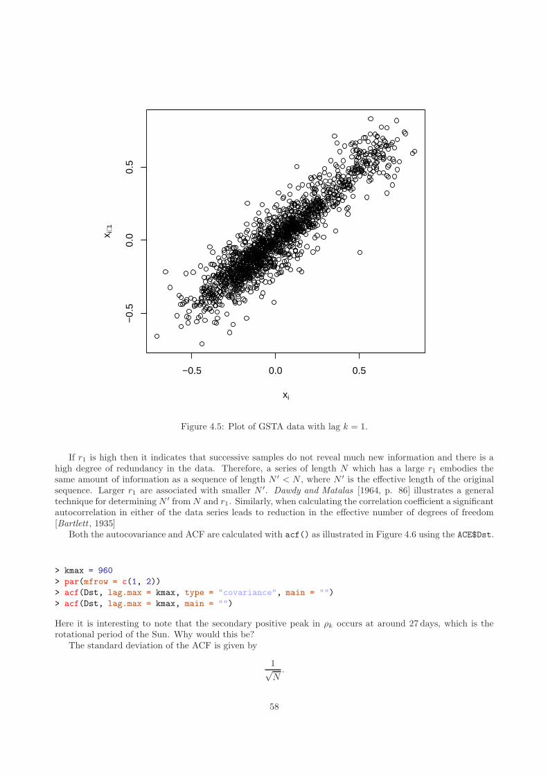
−0.5 0.0 0.5
−0.
50.
00.
5
xi
x i+1
Figure 4.5: Plot of GSTA data with lag k = 1.
If r1 is high then it indicates that successive samples do not reveal much new information and there is ahigh degree of redundancy in the data. Therefore, a series of length N which has a large r1 embodies thesame amount of information as a sequence of length N ′ < N , where N ′ is the effective length of the originalsequence. Larger r1 are associated with smaller N ′. Dawdy and Matalas [1964, p. 86] illustrates a generaltechnique for determining N ′ from N and r1. Similarly, when calculating the correlation coefficient a significantautocorrelation in either of the data series leads to reduction in the effective number of degrees of freedom[Bartlett , 1935]
Both the autocovariance and ACF are calculated with acf() as illustrated in Figure 4.6 using the ACE$Dst.
> kmax = 960
> par(mfrow = c(1, 2))
> acf(Dst, lag.max = kmax, type = "covariance", main = "")
> acf(Dst, lag.max = kmax, main = "")
Here it is interesting to note that the secondary positive peak in ρk occurs at around 27 days, which is therotational period of the Sun. Why would this be?
The standard deviation of the ACF is given by
1√N
.
58

0 1500000 3500000
050
100
Lag
AC
F (
cov)
0 1500000 3500000
0.0
0.2
0.4
0.6
0.8
1.0
Lag
AC
F
Figure 4.6: Autocovariance (left) and ACF (right) of ACE$Dst extending to maximum lag of k = 960 (this isequivalent to 40 days).
On Figure 4.6 the dashed lines indicate the location of the 95% confidence interval (constructed using thestandard deviation). Only peaks that protrude outside these lines are considered to be statistically significantat this level.
4.2.4 Partial Autocorrelation
The partial autocorrelation function (PACF) at lag k, φkk, is the ACF between xi and xi+k with the lineardependence on the intervening data, xi+1 to xi+k−1, removed. Or, equivalently, it is the ACF between xi andxi+k that is not accounted for by lags 1 to k − 1. This may be pictured as follows: suppose that one obtainsthe best linear estimate (in a least squares sense) of xi+k as
xi+k = α1xi+k−1 + α2xi+k−2 + · · ·+ αk−1xi+1,
and similarly for xi asxi = β1xi+1 + β2xi+2 + · · ·+ βk−1xi+k−1
then φkk is simply the conventional ACF between xi − xi and xi+k − xi+k.The PACF is generated using pacf().
> kmax = 240
> pacf(Dst, lag.max = kmax)
This plot is presented in Figure 4.7.
59

0e+00 2e+05 4e+05 6e+05 8e+05
−0.
20.
00.
20.
40.
60.
81.
0
Lag
Par
tial A
CF
Series Dst
Figure 4.7: PACF of ACE$Dst extending to maximum lag of k = 240.
4.3 Stationarity
The major difference between a time series (4.2) and a simple sample (3.1) is the fact that while the order ofthe samples in the latter is completely arbitrary, in the former it is of paramount importance since a definiterelationship exists between successive terms. Although in practice it is generally only possible to make a singleobservation (or at least a finite number of observations) of the time series, in theory this observation is just asingle realisation of the underlying process. If one were able to repeat the process and gather a second timeseries then one would expect it to differ from the first. By repeating the process numerous times one wouldgenerate an ensemble of time series which would characterise the underlying process. The values of the firstsample in each of these time series would have a distribution, which might be denoted P (x1). Similarly thesecond sample would be distributed according to P (x2), while the distribution of xi would be governed byP (xi). Similarly, pairs of successive values would have a distribution of P (xi, xi+1), while sequences of lengthn would be distributed according to P (xi, xi+1, . . . , xi+n+1).
Stationarity is an important characteristic for a time series. A stationary time series is one which hasproperties which are not affected by a change in the time origin. There are different levels of stationarity. Aseries is first order stationary if the distribution of xi is the same as the distribution of xi+k, or P (xi) ≡ P (xi+k).Similarly, a series is stationary to order n if the joint distribution function of the sequence
xi, xi+1, . . . , xi+n+1
is the same as that forxi+k, xi+k+1, . . . , xi+k+n+1,
60

or P (xi, xi+1, . . . , xi+n+1) ≡ P (xi+k, xi+k+1, . . . , xi+k+n+1). A time series is completely stationary if thiscondition applies for all n.
In general the ACF for a stationary time series should drop to zero after a few lags and then oscillateon either side of zero for higher lags. Non-stationary time series are characterised by ACFs which display ahigh level of persistence, decaying only very slowly with increasing lag and exhibiting a smooth pattern ofsignificant values at high lags.
A stationary process has characteristics, such as the mean and variance, which do not change with time.The expectation of xi is
µi = E [xi] .
In principal the expectation of each term in a time series might be different. However, for a stationary processthe distribution of each term is the same so that µi = µ ∀ i. If multiple independent realisations of the timeseries are available then it is possible to estimate E [xi] for each i. With only a single realisation this ensembleaverage is not possible. However, in the case of a stationary time series the time average is equivalent to theensemble average!
A time series which includes a trend thus cannot be stationary. However, there are a few approaches toachieving stationarity in a time series:� differencing and� fitting a curve and then subtracting from the original data.
In the latter case the residuals form the basis of further analysis.
4.3.1 Differencing
To find the difference between successive elements in a time series use diff().
> (x = ts(rnorm(7)))
Time Series:
Start = 1
End = 7
Frequency = 1
[1] 0.427910 1.111592 -1.414378 -0.247309 -1.401148 -0.194359 -0.395877
> diff(x)
Time Series:
Start = 2
End = 7
Frequency = 1
[1] 0.6836823 -2.5259706 1.1670692 -1.1538390 1.2067890 -0.2015180
> diff(x, 2)
Time Series:
Start = 3
End = 7
Frequency = 1
[1] -1.84228830 -1.35890131 0.01323026 0.05295003 1.00527101
Here diff(x) creates a new time series with elements which are xi−xi−1, while diff(x, 2) yields xi− xi−2.The former is the discrete analog of the first derivative. The second derivative is found using
> diff(diff(x))
Time Series:
Start = 3
End = 7
Frequency = 1
61

Time
x
0 20 40 60 80 100
−2
02
46
Time
diff(
x)
0 20 40 60 80 100
−4
−2
02
4
0 5 10 15 20
−0.
20.
20.
61.
0
Lag
AC
F
Series x
0 5 10 15
−0.
50.
00.
51.
0
Lag
AC
F
Series diff(x)
Figure 4.8: Illustration of effect of differencing on the ACF.
[1] -3.209653 3.693040 -2.320908 2.360628 -1.408307
A comparison of synthetic non-stationary data with and without differencing is given in Figure 4.8.
> x <- ts((1:100) / 20 + rnorm(100))
> par(mfrow = c(2, 2))
> plot(x)
> plot(diff(x))
> acf(x)
> acf(diff(x))
Here it is clear that the original data contains a well defined trend and this is reflected by the gradual decayof the ACF. After differencing the trend has been removed and the ACF decays rapidly. To reverse thedifferencing process, use diffinv().
4.4 Missing Data
As we have seen in Section 1.7, data can often be contaminated by missing samples. Although it is possibleto simply exclude the missing samples from the analysis, for example, by using na.rm = TRUE in a call to
62

mean(), it might be more desirable to try and fill in the gaps. Certainly if the gaps are short then this is notan unreasonable thing to do.
Suppose that one had a sequence of values from 1 to 20 and that there were three missing values in thecentre:
> x <- 1:20
> x[10:12] <- NA
> x
[1] 1 2 3 4 5 6 7 8 9 NA NA NA 13 14 15 16 17 18 19 20
To interpolate over the gap one could
> library(zoo)
> na.approx(x)
[1] 1 2 3 4 5 6 7 8 9 10 11 12 13 14 15 16 17 18 19 20
That makes perfect sense. But what if the original data looked like
> x <- c(1:11, 10:1)
> x
[1] 1 2 3 4 5 6 7 8 9 10 11 10 9 8 7 6 5 4 3 2 1
> x[9:13] <- NA
> x
[1] 1 2 3 4 5 6 7 8 NA NA NA NA NA 8 7 6 5 4 3 2 1
Now doing a simple interpolation is just plain wrong.
> na.approx(x)
[1] 1 2 3 4 5 6 7 8 8 8 8 8 8 8 7 6 5 4 3 2 1
Using a spline rather than linear interpolation is a little better but still far from perfect.
> na.spline(x)
[1] 1.000000 2.000000 3.000000 4.000000 5.000000 6.000000 7.000000 8.000000 8.760185
[10] 9.216295 9.368332 9.216295 8.760185 8.000000 7.000000 6.000000 5.000000 4.000000
[19] 3.000000 2.000000 1.000000
So what is the solution? In general it is fairly safe to interpolate over small gaps. But, unless you are reallysure about what the real data looks like, it is better not to try to interpolate over any gaping crevasses in yourdata. Both na.approx() and na.spline() provide a parameter which allows you to specify the widest gapthat will be interpolated.
> x[seq(2, 21, by = 3)] = NA
> x
[1] 1 NA 3 4 NA 6 7 NA NA NA NA NA NA NA 7 6 NA 4 3 NA 1
> na.approx(x, maxgap = 1, na.rm = FALSE)
[1] 1 2 3 4 5 6 7 NA NA NA NA NA NA NA 7 6 5 4 3 2 1
63

4.5 Unevenly Sampled Data
A number of publications [Scargle, 1982, 1989] consider techniques for the analysis of time series which are notsampled uniformly in time.
4.6 Exercises
Exercise 4.1. What is the start, end and frequency of the sunspots data? Extract the portion of data betweenApril 1973 and December 1975. Resample this data quarterly.
Exercise 4.2. Think of some examples of time series data which might posses (i) a trend, (ii) a seasonalvariation, or (iii) both.
Exercise 4.3. With the sunspots data (i) generate the ACF and plot the time series against a lag 1 copy.(ii) What do these plots suggest about the stationarity of the data? (iii) Difference the data and repeat theplots.
Exercise 4.4. Decompose the AirPassengers data assuming that the seasonal component is additive. Repeatwith a multiplicative seasonal component. Is the importance of the type of seasonal component clear?
Exercise 4.5. Decompose the co2 data. Examine the residual to see if there is still any systematic component.
Exercise 4.6. Using the ACE Bx data
(i) create a time series object with appropriate frequency;
(ii) interpolate over missing data;
(iii) generate the ACF. Is there evidence of non-stationarity?
(iv) Increase the maximum lag in the ACF plot to locate the secondary maximum. What does this correspondto?
(v) Difference the data and plot the ACF again.
64

Bibliography
Anderson, O. D., Time Series Analysis and Forecasting, Butterworth & Co (Publishers) Ltd, 1976.
Bartlett, M. S., Some Aspects of the Time-Correlation Problem in Regard to Tests of Significance, Journal ofthe Royal Statistical Society, 98 (3), 536 – 543, 1935.
Chatfield, C., The Analysis of Time Series: Theory and Practice, Chapman and Hall, 1975.
Chatfield, C., The Analysis of Time Series: An Introduction, Chapman and Hall, 1980.
Dalgaard, P., Introductory Statistics with R, second ed., Springer, 2008.
Dawdy, D. R., and N. C. Matalas, Statistical and probability analysis of hydrologic data, Part III. Analysis of
variance, covariance, and time series, chap. 8–III, pp. 8.68—-8.90, McGraw-Hill Book Company, New York,1964.
Maindonald, J. H., Using R for Data Analysis and Graphics, 2008.
Maindonald, J. H., and W. J. Braun, Data Analysis and Graphics Using R - an Example-Based Approach,second ed., Cambridge University Press, 2007.
Meko, D., Applied Time Series Analysis.
Montgomery, D. C., C. L. Jennings, and M. Kulahci, Introduction to Time Series Analysis and Forecasting,Wiley-Interscience, 2008.
Scargle, J. D., Studies in astronomical time series analysis. I. Modeling random processes in the time domain,Astrophysical Journal Supplement Series, 45, 1–71, 1981.
Scargle, J. D., Studies in astronomical time series analysis. II. Statistical aspects of spectral analysis of unevenlyspaced data, Astrophysical Journal, 263, 835–853, 1982.
Scargle, J. D., Studies in astronomical time series analysis. III. Fourier transforms, autocorrelation functions,and cross-correlation functions of unevenly spaced data, Astrophysical Journal, 343, 874–887, 1989.
Shumway, R. H., and D. S. Stoffer, Time Series Analysis and Its Applications: With R Examples, second ed.,Springer, 2006.
Wei, W. W. S., Time Series Analysis, Addison-Wesley Publishing Company, 1990.
Wurtz, D., A. Ellis, and Y. Chalabi, A Discussion of Time Series Objects for R in Finance, 2009.
Zucchini, W., and O. Nenadic, Time Series Analysis with R - Part 1.
65


