Academic Performance in Double-Shift Schooling November 12, 2013 Galiya Sagyndykova 1 Department of Economics, University of Arizona, Tucson, 85721. Abstract Many developing countries with constrained resources have adopted the double-shift school- ing system as a way to serve more students. However, there is some concern that some students may be hurt by these policies. With a unique dataset from Mexico’s National Institute for Ed- ucational Assessment and Evaluation (INEE), I apply Heckman 0 s selection model to measure the effects of individual, teacher, and school characteristics on student test scores and estimate the difference in academic performance of students in morning and afternoon school sessions. While I find a statistically significant effect of being in the morning shift, the Oaxaca decom- position shows that this effect can be explained by the observed difference in characteristics of students from two shifts. The results show that self-selection of students to schooling sessions explains the apparent academic inequality between students from different sessions. 1 [email protected]
Transcript
Academic Performance in Double-Shift Schooling
November 12, 2013
Galiya Sagyndykova 1
Department of Economics,
University of Arizona, Tucson, 85721.
Abstract
Many developing countries with constrained resources have adopted the double-shift school-
ing system as a way to serve more students. However, there is some concern that some students
may be hurt by these policies. With a unique dataset from Mexico’s National Institute for Ed-
ucational Assessment and Evaluation (INEE), I apply Heckman′s selection model to measure
the effects of individual, teacher, and school characteristics on student test scores and estimate
the difference in academic performance of students in morning and afternoon school sessions.
While I find a statistically significant effect of being in the morning shift, the Oaxaca decom-
position shows that this effect can be explained by the observed difference in characteristics of
students from two shifts. The results show that self-selection of students to schooling sessions
explains the apparent academic inequality between students from different sessions.
Double-shift or double-session schooling is a schooling system in which different cohorts of stu-
dents use the same building and have the same academic curriculum, some in the mornings and some
in the afternoons. Many developing countries, including Mexico, India, Brazil, Zimbabwe, Russia,
Bulgaria, have adopted the double-shift schooling system. In the United States, in states such as
Florida, a double-shift system is maintained due to the occurrence of natural disasters affecting the
physical conditions of existing school buildings. In general, the purpose of double-shift schooling is
to increase access to schooling while limiting strain on the budget.
From the policy perspective the introduction of double shifts allows existing sets of buildings
and facilities to serve more students. This may be especially important in urban areas, where
land is scarce and construction of new buildings is expensive. Double-shift schooling has helped
many countries to move toward universal primary and secondary education. However, this policy
may come at a cost. The limited school day under the multiple shift operation leaves few or no
opportunities for any extra-curricular activities. In addition, there is some concern that students
may be hurt by such policy. Afternoon students may receive a poorer education because of their
tiredness by the time of classes or the diminishing productivity of teachers. The purpose of this
study is to determine whether the difference in academic performance of students in the morning
and afternoon shifts has a causal nature or is due to differences in characteristics of students as a
result of the selection process.
Using a unique dataset from Mexico′s National Institute for Educational Assessment and Evalua-
tion (INEE: Instituto Nacional para la Evaluacion de la Educacion ), I examine factors influencing
academic performance of students from different school shifts. More specifically, I focus on ninth
grade students of secondary schools from morning and afternoon shifts and examine the effects of
socio-economic and academic variables on students test score performance. To control for selection
bias I employ the Heckman two-stage model. My key identification for the selection equations comes
from exclusion restriction in which variable restricting school capacity determines the probability
of a student getting into the morning session but not their performance on the tests. Furthermore, I
apply the Oaxaca wage gap decomposition method to decompose the total effect into the effects of
observed characteristics, returns to characteristics, and selection. In addition, I extend the analysis
by decomposing the test difference due to observable characteristics into the three parts: due to the
student, teacher, and school characteristics.
The results of my study reveal that there is no causal effect of the morning shift on the academic
inequality of students from different shifts. Most of the test score difference can be explained by
differences in the characteristics of students. The results also suggest that half of the math test score
1
gap is due to differences in the observed characteristics of teachers. The findings of my research
contribute an argument to the debate addressing the advantages and disadvantages of the double-
shift schooling system. My results suggest that the double-shift schooling in Mexico serves its
purpose by providing the equal education opportunities to all students.
II. Background and Literature Overview
Double-shift schooling (DSS) has been implemented in Mexico since the 1970s as a strategy
to achieve universal access to basic education, given the lack of resources to fund construction
of additional new school buildings. In this way the Mexican government has increased utilization
of existing infrastructure by introducing morning, afternoon, and evening school shifts. Moreover,
teachers have been given the opportunity to hold two teaching positions, thereby increasing their
salaries. However, when schools reach their full capacity and begin to operate in two or three shifts,
schools move away from learning communities where students spend longer periods of time and
engage in extended sessions or extracurricular activities. In addition, the DSS system can create
academic inequality between students from different shifts. In comparisons of means students from
the morning shift perform better than students from the later shifts. The potential explanations for
this difference in academic performance include less productive and/or less qualified teachers, tired
and less attentive students, or negative peer effects in the afternoon shift.
Teachers often want to work to raise their earnings by working in more than one session, which
may affect teacher instruction or teacher productivity. Educators in Mexico have been known as′′taxi teachers′′ because many teachers jump into taxis at the end of the morning session in order to
rush to teach an afternoon session elsewhere if they are not allowed to teach an additional session
at the same school. One implication of ′′shift work′′ by many teachers is that they may be less
effective educators in the afternoon. Unlike many professions where an individual worker performs
a certain task or a few tasks during working hours, teachers must work outside their teaching hours
without extra compensation. Teachers perform multiple tasks requiring specialization in areas such
as educating students, monitoring student performance, and student discipline. In addition, many
duties, such as preparing lesson plans, assignments, and grading, are performed outside the school
and after working hours. Furthermore, teachers are generally required to teach more than one
subject. Given the multiple tasks performed by a teacher, teacher performance may not be constant
over the school day, the semester, or even the entire school year. As a result, a teacher’s diminishing
effectiveness in the classroom may affect students′ performance.
Students who attend the afternoon session spend their mornings studying, or performing house
chores, or working to supplement family income. In rural areas, children generally help their families
in field work. As a result, children attending afternoon school sessions may be at a disadvantage
2
because they are tired and they may be less attentive to new learning.
Because of the perceived difference in academic performance between the different schooling
shifts, goal-oriented parents and students seek the highest quality of education may prefer to attend
the morning school session. However, the morning school sessions cannot accommodate all children.
As a result selection decisions are made by the school administration. In general, student applicants
with higher test scores in earlier year at their elementary schools are given higher priority for
placement into the morning shift. Therefore, the test scores of students from the afternoon shifts,
on average, are lower than the test scores of students from the morning shifts.
The literature on double-shift schooling is presented mostly by education practitioners. Exis-
ting works focus on the issues, problems, and benefits of the multiple shift schooling system. For
example, Brey (2008) provides an overview of double-shift systems for students, teachers and school
administrators. More specifically, Linden (2001) examines secondary schools that teach two sets of
students in two shifts and concludes that double-shift schools appear to offer an adequate education
and a solution for countries with resource constraints seeking to expand their secondary education
systems.
Educational researchers in Mexico have turned their attention to the problems with DSS im-
plementation. By analyzing differences in students′ and teachers′ distributions of characteristics,
Cardenas (2010) found that, on average, afternoon shift schools have lower levels of educational
quality. His research shows that schools in the afternoon session have a higher proportion of low-
income students and higher failure and dropout rates in comparison to morning shift schools sharing
the same facilities. Saucedo Ramos (2005) describes a selection process which intentionally places
repeaters and students with discipline problems into the afternoon session and shows that quality
of instruction is lower in the afternoon than in the morning shift because of the different expecta-
tions and attitudes of teachers and principals. Using aggregate school data, Trevino Villarreal and
Trevino Gonzalez (2004) find the Spanish scores of afternoon cohort students are significantly lower
than the scores of morning shift students. Moreover, they show the importance of positive attitudes
of teachers on the academic performance of students.
The literature on educators focuses on observable teacher characteristics such as experience,
education, and certification. Santibanez (2006) indicates teacher test scores have a small positive
relationship with average student achievement scores, although the effect is larger in secondary
schools than in primary schools. Rivkin, Hanushek, and Kain (2005) find teachers in their first or
second years of teaching are associated with lower student test scores in Texas, but teacher education
and certification have no systematic relationship to student test score achievement. Betts, Zau, and
Rice (2003) find mixed results for teacher characteristics using detailed individual-level data from
3
elementary schools in the San Diego Unified School District. Rockoff (2004) shows teacher quality,
measured by teacher fixed effects, have an important impact on student achievement. In other
words, teacher quality may be important for students’performance; however, teacher productivity
may be a detriment to students’performance when teachers work extended hours.
III. Education System in Mexico
According to the Constitution of Mexico, the objective of Mexican public education is compul-
sory education free of charge for every child. Since the Mexican Revolution of 1917, the basic goal
of the government has been to increase educational coverage. Today, the Mexican education sys-
tem serves over 30 million students and employs 1.6 million teachers in more than 229,000 schools
and basic education enrollment has more than doubled from 9.7 million students in 1970 to 21.6
million students in 2000 (Razquin, Santibanez , Vernez (2005)). This rapid growth in basic educa-
tion demand is primarily met by double shifting of schools and flexibility of teacher employment
practices.
The Mexican education system is organized into four levels: preschool (K1–K3), compulsory
basic education (grades 1–9), which includes primary and lower secondary education, upper secon-
dary education (grades 10–12), and higher education. The government is officially responsible for
providing compulsory basic education. The education system of Mexico also allows for the exis-
tence of private schools, but the public school system serves almost 90 percent of all students in
the country. The delivery of basic education in Mexico takes different forms. However, ninety-three
percent of primary education is delivered by general modality, a traditional approach that employs
the Ministry of Education pre-approved universal national curriculum.
The Ministry of Education of Mexico (SEP: Secretarıa de Educacion Publica ) is responsible for
the country′s educational system; which includes setting guidelines for teacher salaries, along with
the academic calendar year and the length of the school day. Specifically, all teachers are required
to follow SEP′s national curriculum. Primary schools must use national textbooks, while secondary
schools must choose textbooks from a nationally approved list. The school calendar generally is
set to 200 days, beginning in August and ending in June of each calendar year. SEP specifies the
length of each school day to four hours, allowing primary schools to operate regular sessions in
multiple shifts: morning, afternoon, and sometimes evening. On the other hand, lower secondary
schools operate in the mornings and afternoons, and each shift meets for five hours. In each regular
shift, one-hour subjects include Spanish, mathematics, natural sciences, and social sciences. The
consequences of operating multiple shifts and a limited school day leave few or no opportunities to
study music or participate in extra-curricular activities such as sports, although some schools do
make time for these subjects.
4
IV. Identification Strategy
A. Main Model Framework
To identify factors that influence the academic performance of students, this study employs a
model developed by Nakosteen and Zimmer (1980) to estimate migration decisions, using Heckman’s
(1979) two-stage estimation technique for sample selection bias. Specifically, the students in the
sample are categorized into one of these two mutually exclusive regimes, with the selection equation
serving as an endogenous selection criterion which determines the student′s shift.
Unlike the Nakosteen and Zimmer model, in which the migration decision is voluntary and based
on an implicit cost-benefit analysis, this study’s sorting function between morning and afternoon
shifts involves both the choice of a student and the decision of the school administration. For
simplicity, the analysis assumes every child (or their parents) prefers the morning shift, ceteris
parabus. Although this assumption might not be completely true and there may be students who
prefer the afternoon shift, the assumption is close to reality. One the instances of these reasons is the
working schedule of parents. However, the fact that on average morning session grades are higher
than afternoon grades makes the morning shift more desirable for students. In addition, the quality
of teaching may be better in the morning, because teachers may not yet be tired, and therefore
more effective in their teaching. As a result, excess demand for and limited capacity in the morning
shift force students who cannot get into the morning cohort to be enrolled in the afternoon session.
In fact, the unbalanced cohort size in the data reflects this situation.
Formally, at the beginning of middle school, student i wants to get into the morning shift if
Si(Mi|Xi)− Si(Ai|Xi) > Fi,
where S(·) is the score function of a student’s family, representing the utility of schooling, M is an
indicator variable that equals 1 if student i is in the morning shift and 0 otherwise, A = 1−M , and
X represents student, teacher, and school characteristics. The function F represents opportunity
costs of the morning shift as a difference in expected scores. Furthermore, this function, which is
assumed to be linear and additive, can be expressed as a function of characteristics, X, and an error
term, v:
Fi = f(Xi) + vi (1)
Though the capacity for both shifts is the same when both shifts use the same schooling facilities,
the school selection process in the morning session fills up to full capacity. Therefore, the enrollment
in the morning shift, Em, is equal to the full capacity of the school and the enrollment in the
afternoon shift, Ea is less than or equal to the maximum capacity of the school. Since school
5
capacity is different across schools, the ratio of morning to afternoon enrollment represents the
degree to which capacity is constrained forthe morning session. In other words, W = Em
Eagiven the
observed school characteristics should determine the probability that a student is admitted to the
morning session. The sorting function can be modeled as
Prob(Mi = 1|Xi,Wi) = Φ(Z ′iγ) (2)
where Wi ≥ 1 and Zi = (Xi,Wi).
Given the selection mechanism for students into the morning shift, the sorting equation is the
function of gains in shifts′ scores and student, teacher, and school characteristics. Specifically, stu-
dent i, with the vector of explanatory variables and excluded variables in the vector Zi gets into
the morning shift if
M∗i > 0
and the afternoon shift if
M∗i ≤ 0
where
M∗i = α0 + α1(Smi − Sai) + Z ′iα2 − εi (3)
The model is completed by the test score equations for morning and afternoon students as
follows:
Smi = X ′miβm + umi (4)
Sai = X ′aiβa + uai, (5)
where Sm and Sa are the performance scores for morning and afternoon students. The unobserved
error terms ε is assumed to be a standard normal variable and um, ua are unobserved error terms
with means 0 and variances σ2m and σ2
a. In addition, the disturbance terms in equations (3), (4),
and (5) are assumed to be jointly normally distributed with zero means and nonzero correlation
between ε and um, ε and ua.
We observe an indicator variable for the morning shift, defined as M = 1 if M∗i > 0 and M = 0
if M∗i ≤ 0. In addition, we observe the scores for students in this certain shift, or S = Sm when
Mi = 1 and S = Sa when Mi = 0.
Substituting equations (4) and (5) into equation (3) yields a reduced form of the sorting equation:
M∗i = γ0 + Z ′iγ1 − νi (6)
6
where Z is the vector consisting of all exogenous variables in the model for both groups of students.
Assuming that ν is normally distributed with mean zero and unit variance, the sorting equation
above is estimated by the probit model.
Then, if we define ψi = γ0 + Z ′iγ1, the conditional means of the score disturbance terms do not
equal zero, but vary with each observation, and differ for the morning and the afternoon cohort:
E(umi|Mi = 1) = ρumεσum
[−φ(ψ)
Φ(ψ)
](7)
E(uai|Mi = 0) = ρuaεσua
[ φ(ψ)
1− Φ(ψ)
], (8)
where ρuε is the correlation between morning or afternoon respective u and ε, σum and σua are the
standard deviations of the disturbance terms of the two main score equations, and φ(·) and Φ(·)are the standard normal density and cumulative distribution functions, respectively.
B. Estimation Technique
The estimation of the score equations employs the ′′Heckman Two-Step′′ methodology. The first
step runs a probit regression of the reduced form sorting equation (6) using all observations from
both morning and afternoon shifts. The estimate of γ from the probit estimation is then used to
obtain fitted values of ψi to construct consistent estimates of the Inverse Mills Ratio (IMR) for the
morning shift
λmi =[−φ(ψi)
Φ(ψi)
]and afternoon shift
λai =[ φ(ψi)
1− Φ(ψi)
].
In the second stage, the outcome equations, including the IMR variable, are estimated by OLS
technique, where the score equations are:
Smi = X ′miβm + θmλmi + ηmi (9)
Sai = X ′aiβa + θaλai + ηai (10)
C. Test Score Gap Decomposition
Heckman′s two-stage estimation technique consistently estimates the parameters of the score
equations. The unbiased estimators of the score equations can further be used to estimate the average
expected score difference across students in different shifts. However, even after the selection bias
7
correction, the average test score difference cannot explain the reasons why this difference still exists.
The selection process allows us to see that on average the morning student is endowed with better
characteristics. This might create unobservable peer effects. On the other hand, it is possible that
differences in teacher characteristics can reinforce the positive effect of the academically advanced
morning students or that the effect night be negated by the effect of bigger classes. In order to
identify the nature of the test score gap I apply the methodology of Neuman and Oaxaca (2004) to
the difference in expected test scores from different sessions.
The difference in expected values of test scores of the morning and afternoon shifts for a students
i is:
τi = E(Smi|Xmi,Wi,Mi = 1)− E(Sai|Xai,Wi,Mi = 0)
= [X ′miβm + θmλmi]− [X ′aiβa + θaλai]
Then the estimate of the overall difference in expected scores of different shifts, τ , is
τ =1
n
n∑i=1
τi = (X′mβm −X
′aβa) + (θmλm − θaλa) (11)
where X is the mean vector of score determining the variables including a constant term, β is the
vector of the estimated returns to the score determinants, θ is the estimate of ρuεσu, and λ is the
mean of the Inverse Mills Ration estimated from the first stage of the selection equation.
Furthermore, the decomposition technique identifies the difference in the average scores between
sessions due to the difference in characteristics, or explained gap, due to the returns to characteristics
of students, teachers, and schools, or unexplained, and due to the selection process.
τ = (Xm −Xa)′βa︸ ︷︷ ︸
explained gap
+X′m(βm − βa)︸ ︷︷ ︸
unexplained gap
+ (θmλm − θaλa)︸ ︷︷ ︸gap due to the selection
(12)
The explained gap, or the difference in expected score due to the difference in observed charac-
teristics, can be further decomposed into the difference due to the students, teachers, and school
characteristics.
(Xm −Xa)′βa = (Xm,student −Xa,student)
′βa,student
+ (Xm,teacher −Xa,teacher)′βa,teacher
+ (Xm,school −Xa,school)′βa,school
Such fine decomposition can explain the exact source of the the difference in score gap if any.
8
V. Data Description
This paper employs the INEE dataset of standardized tests, administered by the SEP of Mexico
to assess the general level of knowledge of students in both public and private schools throughout the
country. The INEE was created by a presidential mandate on August 8th, 2002 as an independent
organization to monitor and to assess the quality of the National Educational System.
The INEE collects information and conducts surveys to evaluate the students educational achie-
vement and the general quality level of schools. The INEE collaborates with the The Organization
for Economic Co-operation and Development (OECD) in the Programme for International Student
Assessment (PISA) since 2000 and with the United National Educational, Scientific and Cultu-
ral Organization (UNESCO) in Second Regional Comparative and Explanatory Study (SERCE)
since 2006. For the national education evaluation, the INEE developed Reviews of Quality and
Educational Achievement (EXCALE: Examenes de la Calidad y el Logro Educativos ) in 2004.
The paper employs EXCALE–09. EXCALE–09 are datafiles containing a representative sample
of ninth graders from lower secondary schools at the end of the 2007-2008 school year. The ninth
grade signifies the last year for compulsory education; thereafter students have the option either
to continue their education at the high school level or to end their schooling and enter the labor
market.
The INEE administers paper-and-pencil tests to all ninth-grade students. The test format com-
bines multiple-choice and open-ended questions. The test results are normalized and between 200
and 800. In addition to student test results, the INEE conducts survey questionnaires on personal
characteristics with students, teachers, and school principals. Each student, teacher, and school is
assigned a unique identifying code in the EXCALE dataset. Using these identifying codes I merge
student test scores with their survey questionnaires. Personal student questionnaire contains many
questions which allows me to pick a number of student characteristics to identify the parameters
of their test score equations and control for the self selection as well as the identifying code of
the school the student is in. Specifically, student characteristics include a student′s gender, age,
parentsıncome, whether she lives with one or both parents, educational level of the student’s pa-
rents and their occupational category, average number of hours a week the student spends studying
outside of school, and whether the student is required with house chores.
Datasets containing the questionnaire answers of teachers and school principals have the school
code that allows me to merge these datasets with the student information. The rich questionnaires
allow me to handpick the teacher variables, such as her age, education level, and experience, the
total number of hours the teacher works at a given school, whether she teaches one subject or more,
and whether she teaches another shift or is employed outside of education.
9
Variables capturing the average number of hours a week a student spends helping her family, a
dummy variable for whether a teacher teaches another shift or has another job. This variable may
reveal whether a teacher teaching an additional shift diminishes teacher productivity and, thus,
may be less effective as a teacher. In addition,when a child spends time helping the family it may
cause a student to be fatigue and, thus, less attentive in the classroom.
The variables determining the probability that a student gets into the morning shift is the relative
constraining capacity of the morning shift school, Em
Ea. Since the number of students applying to
the morning shift exceeds the capacity of the morning session, morning session enrollment must be
higher than afternoon shift enrollment. The Ministry of Education statistical data support this fact.
On average, the ratio of urban school morning shift enrollment to afternoon enrollment sharing the
same facilities is 2.18 with a standard deviation of 1.63.
The enrollment data for each school and other variable describing school characteristics are
available in the principal′s questionnaire. Each different shift is assigned a unique, untraceable
identification number. In other words, two different shifts sharing the same school building have
two different identification numbers. As a result, it is not possible to identify in the INEE data
whether two shifts are using the same school building. Using the publicly available data on Mexican
schools I constructed a variable for constraining capacity of the morning shift, Wi. Upon special
request, the research office of the INEE matched this variable to each school shift sharing the same
building.
The excluded variable W for student i captures the morning shift enrollment constraint of a
student’s school relative to the afternoon shift enrollment. In other words, for the morning session
students, the probability of getting into the morning shift increases in Wism, holding everything else
constant. Similarly, for students in the afternoon session, the exclusion restriction Wisa decreases in
their school enrollment relative to the average morning enrollment. So, the probability of getting
into the morning shift increases in Wisa. These excluded variables do not directly correlate with
the academic performance of students. The school size and number of schools in the area depend
on the local government budget and are therefore exogenous in the model. However, there may be
worries that the shift enrollment correlates with the test scores, the outcome variable, through the
class size or school quality. For instance, Angrist and Lavy (1999) find reducing class size induces
an increase in test scores for fourth and fifth graders. Card and Krueger (1992) suggest reduction
in the student-teacher ratio for elementary school students results in an increase in test scores on
reading and math exams. Hence, school enrollment might be large or small, but potential success
in a course strongly depends on the number of students in a class, or the teacher-student ratio. In
order to control this potential correlation, a class size variable as a part of teacher questionnaire is
10
included as a control variable in the analysis.
Other variables determining the school quality, such as the numbers of books and computers in
the school, the existence of violence activity in the vicinity of the school, whether a school equipped
for disabled students, if there is sport facility in a school, and if a school in the urban area are also
included in the estimation. Therefore, holding school quality constant, the excluded variable W can
serve as the determinant for sorting students into shifts.
The process of merging multiple datasets identified matching codes for only math and Spanish
reading comprehension scores. The final samples for the analysis includes only students from public
schools of general modality using double-shift system. Therefore, the compiled dataset for this
study includes final math score sample of 2,579 students and the final Spanish score sample of 2,532
students with 1,367 and 1,308 students in the morning shift, respectively.
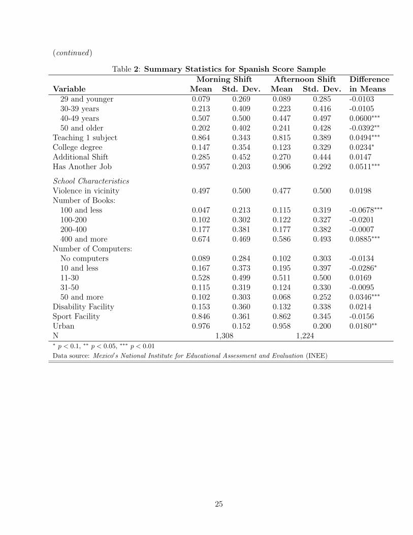
Summary statistics are reported in Tables 1 and 2. Since the data comes from the survey
questionnaire the answers are categorical. Most of categorical answers are not linear in their values.
In order to avoid any measurement errors and censoring problems in the analysis all variables are
converted into the set of indicator variables. The first four columns of the table show the mean and
the standard deviation of variables for morning and afternoon sessions. The last column reports the
t-values for the test if the variables′ means of two groups of students are equal. The t-statistics show
that most characteristics of morning group of students are very different from the characteristic of
afternoon students. Specifically, morning students have higher average test score both in math and
Spanish. They are younger than afternoon students which shows that there are more repeaters in
the afternoon session who are less likely to get into the morning shift. Students from the morning
shift come from the wealthier families and whose parents are more educated and work in the more
professional positions. We can also see that morning classes are bigger on average and have more
experienced teacher. Although, the summary statistics also shows that morning teachers are more
likely to teach another shift and work more hours.
VI. Regression Results
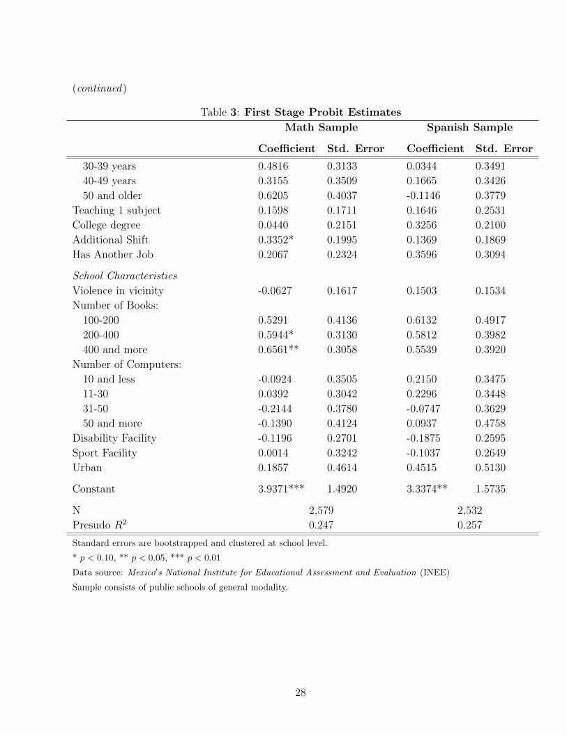
The first stage of the Heckman procedure involves estimation of a probit equation, where the
dependent variable takes on the value 1 if the student is in the morning session and 0 if the student
is in the afternoon session. Table 3 presents the results of this estimation on the math and Spanish
samples respectively. The parameter of the constraining capacity of the morning school is positive
and statistically significant for mathematics and Spanish scores. This implies the probability of
getting into the morning shift increases with the increase in the constraining enrollment of a school,
conditioning on a student and school characteristics. The sign of this excluded variable is as predicted
by the model. In addition, the Chi-square test from the probit estimation indicates the assignment
11
of students into various schooling shifts is not random. The estimates from the probit regressions
are used to construct the Inverse Mills Ratio (IMR) to correct for selection bias in the estimation
of the score equations.
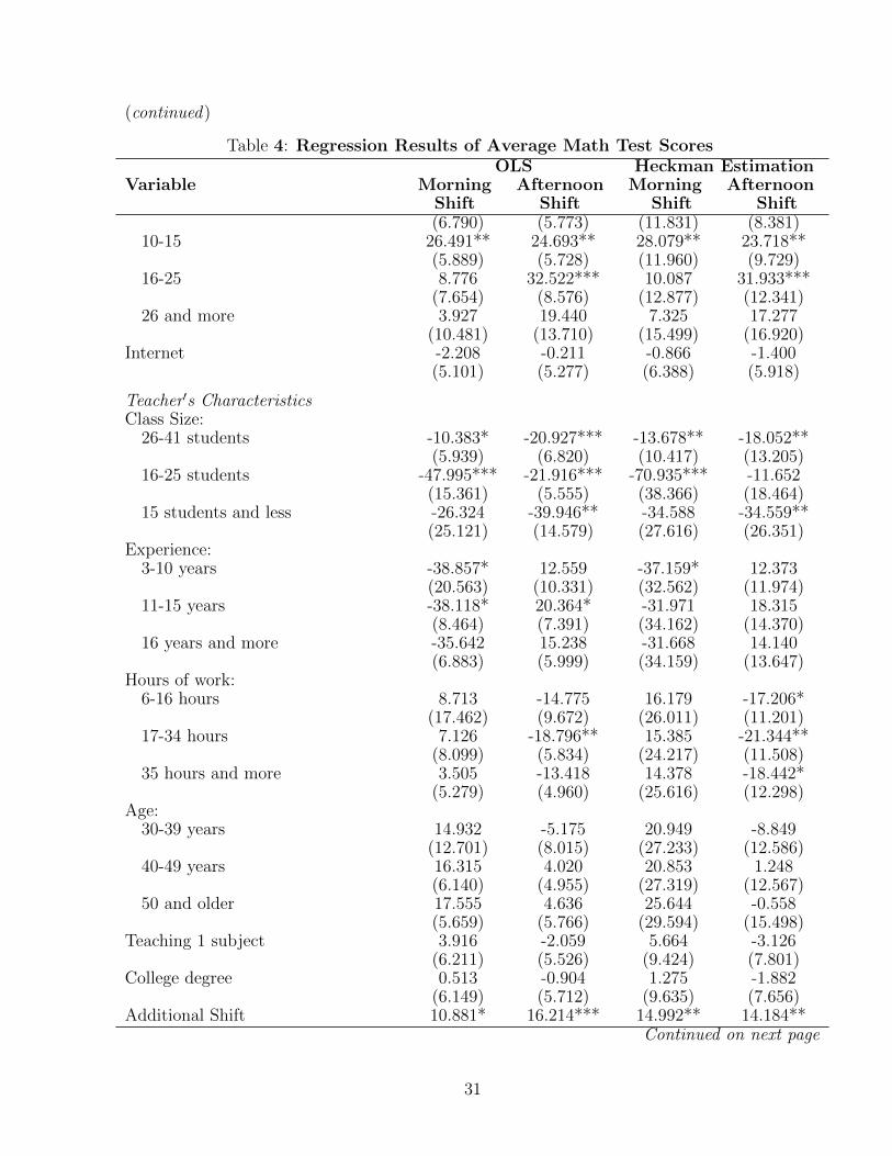
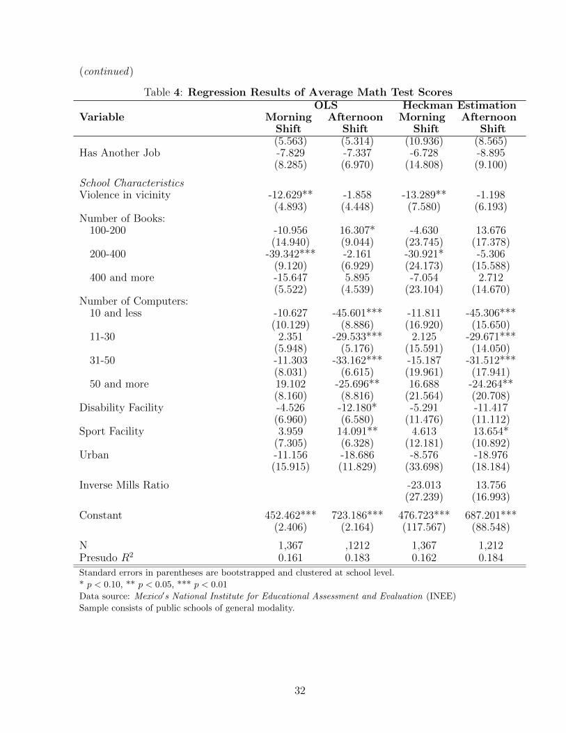
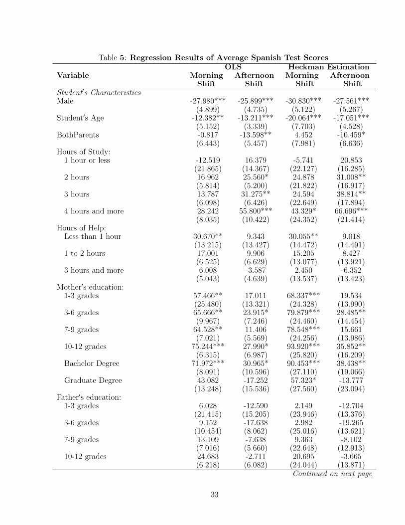
Tables 4 and 5 report the estimated score equations on math and Spanish samples respectively.
The first two columns present the results of the least square regressions, and other two columns
present the results of the regressions with selectivity correction. Although, the coefficients on the
IMR are not statistically significant the IMR still takes care of the selection into the shifts.
A number of the estimated coefficients on the variables of some categories that explain scores
for the difference between two schooling shifts are not statistically significant. However a teacher
teaching another shift has a positive effect on the math scores of students. This variable has less
positive effect on the Spanish performance and the result is statistically significant only for morning
session students. The sign of this variable is not as it was expected. This might be explained by the
fact that a teacher teaching another shift gets a chance to practice his lecture more and presents it
better. Interestingly, the teacher’s hours of work has a negative effect on afternoon student’s math
score. This might be an evidence of the teacher′ diminishing productivity. However, the variable for
a teacher working more than 35 hours a week has a positive influence on Spanish scores. A student
spending more than three hours a week helping around the house has lower Math and Spanish scores
in the afternoon shift although the effect is not statistically significant. Math score is higher for a
students spending more time studying at home. Moreover, the magnitude for morning students is
larger than for afternoon students. The same variable has also a positive effect on the Spanish score
of students studying more hours a day, but the effect is larger for afternoon students.
The coefficient of the dummy variable for male students is positive and statistically significant in
the Math equation and negative and statistically significant in the Spanish equation. This indicates
that boys perform better in mathematics tests while girls perform better on tests of literacy and
writing, which is consistent with the literature. Zembar and Blume (2009) show girls, on average,
are better at spelling than boys and perform better on tests involving literacy, writing, and general
knowledge, while boys, on average, perform better on mathematics tests in fourth grade.
Although no direct measure of a student family income exists in the dataset, a proxy variable
is generated from the number of light bulbs and availability of internet access. Specifically, Sathaye
and Meyers (1985) argue that wealthy families in developing countries live in larger homes and
demand greater lighting of their houses than low-income households. In this study the number of
light bulbs in a house, is positive and statistically significant for the families with 10 light bulbs and
higher in a house, which is generally consistent with the results of other studies revealing the positive
relationship between income and academic performance. The age of student coefficient is negative
12
and statistically significant for the students in the afternoon shift, which indicates that students
older than average ninth grader perform worse. Also, considering the selection process of students
into the shifts, repeaters, or students older than their peers, are more likely to be in the afternoon
shift. Therefore, the student’s age has such a negative impact on the academic performance in the
afternoon session.
Davis-Kean (2005) establishes a relationship between parents′ educational attainment and children′
academic achievement through parents′ educational expectations and parent-specific behaviors. My
results show that mother’s education has positive and statistically significant effect on academic
performance of students rather than father’s education. There is more effect of mother’s education
on math scores of morning students while there is no evidence of the effect on afternoon shift stu-
dents. On the other hand, Spanish scores are positively related with the education of a mother in
both shifts, although the magnitude of the effect is higher for morning students.
Larger class size has a more negative impact on math test performance than on Spanish. This
may be explained by the difference in the nature of two subjects: math needs more concentration
and individual approach which is less possible in beggar classes. Card and Krueger (1992) also show
rate of returns to education are higher for individuals from states with better-educated teachers
and with a higher fraction of female teachers. Although a number of studies show mixed results
from a teacher′s experience on a student′s achievement scores, the less experienced teachers in this
study show a positive effect on afternoon students′ performance in Spanish and negative effect on
morning students′ performance in math.
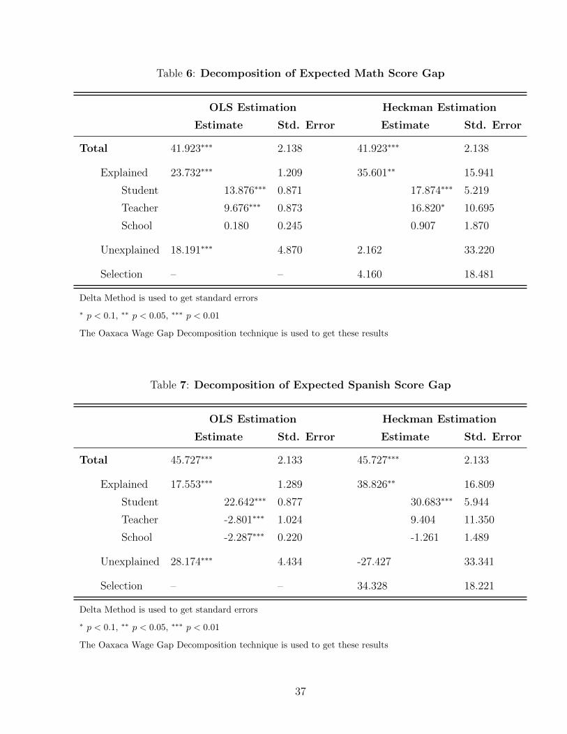
The predicted total average score gap along with its decomposition are presented in Tables 6
and 7. The left panels of each table show the decomposition of the effect of the morning shift using
a simple OLS specification. Uncorrected for selection, results show the average difference between
morning and afternoon students. On average, morning students score about 42 points higher on
math and about 46 points higher on Spanish reading comprehension tests which roughly translates
to about 8 percent of the mean morning score. The decomposition results imply that not all of
the difference is due to the unobserved effect of the school shift. More than a half of the score gap
is explained by the differences in the observed characteristics of students, teachers, and schools.
Moreover, the further decomposition of the explained gap shows us that the statistically significant
effect is due to the difference in students and teachers variables.
The right panel of both tables presents the decomposition results corrected for the selection.
Even though the results show students on average do better in the morning session than in the
afternoon, the difference due to the returns to characteristics is not statistically different from zero.
In other words, there is no evidence that the academic performance of students would be better in
13
the morning school if students were randomly assigned to the different shifts. The implication is
that most of the positive effect of going to the morning session may be due to the fact that better
students get to the morning shift due to the assignment process. Most of this effect come from the
difference in the observed characteristics, specifically from the characteristics of students. Of the
total math score difference, about 17 points, or 3 percent of the mean morning math score can be
explained by the difference in the characteristics of teachers, while Spanish scores do not depend
on teacher characteristics. Math is the harder subject to teach and this may explain the greater
importance of teacher. In both subjects the selection component of the test score gap is positive,
although is not statistically significant.
The results indicate that if there were no difference in the characteristics of the average student
from the morning and afternoon shifts, there would be no statistically significant effect of the
morning shift. That is, the non-random assignment of the students into the shifts may be the
reason of the apparent academic inequality between these two group of students. However, if the
students were to be assigned to the shifts randomly, the difference between two schooling shift my
be eliminated
VII. Conclusion
The double-shift schooling system has been widely used to expand student enrollments and
thereby to achieve the objective of ′′Education for All.′′ Despite the advantages of the double-shift
schooling system, there may be negative externalities in academic achievement between the students
from different schooling sessions. For instance, teacher effectiveness may decrease in the afternoon
shift; which may lead to a reduction in the quality of teaching. In addition, students′ concentration
may be lower in the afternoon, which in turn may affect the ability to learn new material and, thus,
result in lower academic performance by students in the afternoon shift.
This paper examines the double-shift schooling system in Mexico, where the school administra-
tion assigns children to the different schooling sessions. The non-random assignment of children to
different schooling shifts results in differences in the performance score gap between students in the
morning and in the afternoon shifts. As a result, high ability students are granted admission into
the morning shift, while low ability students are assigned to the afternoon session. As a result, these
factors could result in an unequal distribution of educational opportunities across different groups
of students.
This study analyzes academic performance of students from different schooling shifts using the
Heckman selection model. The findings show a teacher working more hours yields a negative effect
on students performance in both shifts. In addition, student studying is positive and statistically
significant in the morning shift. However, most of the effect of the morning shift on academic
14
achievement is due to the difference in the characteristics of students. In other words, the random
assignment of students to the different schooling sessions may help to eliminate apparent average
difference in the performance scores.
The importance of this research contributes to the debate of public policies and, moreover, the
ways that government institutions address the consequences of the double-shift schooling system.
In the case of Mexico, the double-shift schooling provides a solution to issues related to scarce
resources and infrastructure limitations without creating inequalities in the quality of the education
students receive between the two sessions.
15
VIII. References
1. Angrist, J., Lavy, V. (1999). Using Maimonides′ Rule to Estimate the Effect of Class Size on
Scholastic Achievement. The Quarterly Journal of Economics, 533–575
2. Bergman, H. (1996). Quality of Education and the Demand for Education – Evidence from
Developing Countries. International Review of Education, Vol. 42(6), 581–604.
3. Betts, J., Zau, A., Rice, L. (2003). Determinants of Student Achievement: New Evidences
from San Diego. Public Policy Institute of California, San Francisco.
4. Blume, L. B., Zembar, M. J. (2009). Middle Childhood Development: A Contextual Approach.
Allyn & Bacon, an imprint of Pearson Education Inc., 212–215.
5. Brey, M. (2008). Double-Shift Schooling: Design and Operation for Cost-Effectiveness. 3rd
Edition. Paris: UNESCO: International Institute for Educational Planning
6. Brey, M. (1990). The economics of multiple-shift schooling: Research evidence and research
gaps. International Journal of Educational Development, Volume 10, Issues 2-3, 181–187
7. Cardenas, S. (2010). Separados y Desiguales: Las Escuelas de Doble Turno en Mexico. Centro
de Investigacion y Docencia Economicas, February.
8. Card, D., Krueger, A. B. (1992). Does School Quality Matter? Returns to Education and the
Characteristics of Public Schools in the United States. Journal of Political Economy, Vol. 100,
F1F40.
9. Carrell, S. E., Maghakian, T., West, J. E. (2010). A’s from Zzzz’s? The Causal Effect of
School Start Time on the Academic Achievement of Adolescents. American Economic Journal:
Economic Policy, No. 3(3): 62–81.
10. Clotfelter, C. T., Ladd, H. F., Vigdor, J. L. (2003). Teacher sorting, teacher shopping, and
the assessment of teacher effectiveness. Unpublished manuscript, Duke University.
11. Corak, M., Lauzon, D. (2009). Differences in the Distribution of High School achievement:
The Role of Class-Size and Time-in-Term. Economics of Education Review, 28, 189198.
12. Cortes, K., Bricker, J., Rohlfs, C. (2012). The Role of Specific Subjects in Education Pro-
duction Functions: Evidence from Morning Classes in Chicago Public High Schools. The B.E.
Journal of Economic Analysis and Policy, 12(1). Article 27.
16
13. Davis-Kean, P. E. (2005). The Influence of Parent Education and Family Income on Child
Achievement: The Indirect Role of Parental Expectations and the Home Environment. Journal
of Family Psychology, Vol. 19, No. 2, 294–304
14. Dee, T. (2005). Teachers and the Gender Gaps in Student Achievement. NBER Working
Paper, No. 11660.
15. Dills, A. K., Hernandez-Julian, R. (2008). Course Scheduling and Academic Performance.
Economics of Education Review, 27, 646654.
16. Edwards, F. (2012). Early to rise? The Effect of Daily Start Times on Academic Performance.
Economics of Education Review, Vol.31: 970–983
17. Epple, D., Romano, E., Sieg, H. (2003). Peer Effects, Financial Aid and Selection of Students
into Colleges and Universities: an Empirical Analysis. Journal of Applied Econometrics, Vol.
18, 501–525.
18. Hanushek, E. (1971). Teacher characteristics and gains in student achievement: estimation
using micro data. American Economic Review, 61, 280–288.
19. Heckman, J.J. 1979. Sample Selection Bias as a Specification Error. Econometrica, 47(1): 153–
61. Jepsen, C. (2005). Teacher characteristics and student achievement: evidence from teacher
surveys. Journal of Urban Economics, 57, 302–319
20. Kodde, D. A., Ritzen, J. M. M. (1988). Double-Shift Secondary Schools: Possibilities and
Issues. World Bank, Human Development Network Secondary Education Series.
21. Krueger, A. B. (2003). Economic Considerations and Class Size. The Economic Journal, Vol.
113, Issue 485, F34-F63.
22. Linden, T. (2001). Using Maimonides Rule to Estimate the Effect of Class Size on Children′s
Academic Achievement. Quarterly Journal of Economics, Vol. 114 (May), F533F75.
23. Meyers, S., Sathaye, J. (1985). Energy Use in Cities of the Developing Countries. Annual
Review of Energy, Vol. 10, 109–33.
24. Murnane, R. (1975). The Impact of School Resources on the Learning of Inner City Children.
Ballinger, Cambridge, MA.
25. Nakosteen, R.A. and Zimmer, M. (1980). Migration and Income: The Question of Self−Selection.
Southern Economic Journal 46(3): 840–851
17
26. Newey, W. K., Powell, J. L., Walker, J. R. (1990). Semiparametric Estimation of Selection
Models:Some Empirical Results. The American Economic Review, Vol. 80, No. 2, 324-328.
27. Newey, W. K. (2009). Tow-step Series Estimation of Sample Selection models. Econometrics
Journal, Vol. 12, S217–S229.
28. Oaxaca, R. L. (1973). Male-Female Wage Differentials in Urban Labor Markets. International
Economic Review, Vol. 14, 693–709.
29. Oaxaca, R. L., Ransom, M. (1998). Calculation of Approximate Variances for Wage Decom-
position Differentials. Journal of Economic and Social Measurement, Vol. 24, 55–61.
30. Oaxaca, R. L., Neuman, S. (2004). Wage Decompositions with Selectivity–Corrected Wage
Equations: A Methodological Note. Journal of Economic Inequality, Vol. 2, No. 1, 3–10.
31. Palafox, J. C., Prawda, J., Velez, E. (1994). Primary School Quality in Mexico. Comparative
Education Review, Vol. 38, No. 2, 167-180.
32. Razquin, P., Santibanez , L., Vernez, G. (2005). Education in Mexico: Challenges and Oppor-
tunities. RAND Education.
33. Rivkin, S., Hanushek E., Kain J. (2005). Teachers, schools, and academic achievement. Eco-
nometrica, Vol. 73, No. 2, 417–458.
34. Robinson, G. E. (1990). Synthesis of Research on the Effects of Class Size. Arlington, VA:
Educational Research Service.
35. Rockoff, J. E. (2004). The impact of individual teachers on student achievement: evidence
from panel data. American Economic Review, 94, 247–252.
36. Santibanez , L. (2006). Why we should care if teachers get A′s: Teacher test scores and student
achievement in Mexico. Economics of Education Review, 25, 510–520.
37. Saucedo Ramos, C. (2005). Los Alumnos de la Tarde son los Peores: Practicas y Discursos
de Posicionamiento de la Identidad de slumnos Problema en la Escuela Secundaria. Revista
Mexicana de Investigacion Educativa, 10(26), 641-668.
38. Trevino Villarreal, E., Trevino Gonzalez, G. (2004). Estudio sobre las desigualdades educativas
en Mexico: la Incidencia de la Escuela en el Desempeno Academico de los Alumnos y el rol
de los Docentes. INEE,February.
18
39. Willis, R. J., Rosen, S. (1979). Education and Self-Selection. Journal of Political Economy,
Vol. 87, No. 5.
40. Uwaifo, V. O. (2008). The Effects of Family Structure and Parenthood on the Academic
Performance of Nigerian University Students. Studies on Home and Community Science, Vol.