Accelerated Lattice Boltzmann Model for Colloidal Suspensions || Hybrid LBM for Surfactant-Covered...

Chapter 4

Hybrid LBM for Surfactant-Covered

Droplets

Abstract This chapter describes a novel hybrid lattice Boltzmann model for the

study of the droplet flow behavior in an immiscible medium with insoluble nonionic

surfactant adhering to its interface. The evolution of the surfactant concentration on

the interface is modeled by the time-dependent surfactant convection-diffusion

equation and solved by a finite difference scheme. The fluid velocity field, the

pressure, and the interface curvature are calculated using the lattice Boltzmann

method (LBM) for binary fluid mixtures. The coupling between the LBM and the

finite difference scheme is achieved through the LBM macroscopic variables and

the surfactant equation of state. The Gunstensen LBM is used here because it

provides local and independent application of a distinct interfacial tension on the

individual nodes of the droplet interface. The hybrid model is developed and

successfully applied to droplets deformations and surfactant distribution under

simple shear flow, uniaxial flow, and buoyancy.

This chapter aims at adding a humble contribution to the wealth of several numer-

ical methods proposed by some devoted researchers for the study of surfactant

covered drop’s behavior under diverse flow conditions. The work represents an

expansion of the Gunstensen model applicability to cover the study of immiscible

droplets with nonionic insoluble surfactant adhering to their interfaces. Adding the

surfactant effects on the Gunstensen model is facilitated by the ease in the initial-

ization and the tracking of the surfactant concentration on the interface, which

location is well defined in the LBMmodel at each time step, and by the independent

local application of a nonisotropic interfacial tension on the droplet external

surface.

Electronic supplementary material Supplementary material is available in the online version of

this chapter at http://dx.doi.org/10.1007/978-1-4899-7402-0_4. Videos can also be accessed at

http://www.springerimages.com/videos/978-1-4899-7401-3

H. Farhat et al., Accelerated Lattice Boltzmann Model for Colloidal Suspensions:Rheology and Interface Morphology, DOI 10.1007/978-1-4899-7402-0_4,© Springer Science+Business Media New York 2014

69

http://dx.doi.org/10.1007/978-1-4899-7402-0_4

http://www.springerimages.com/videos/978-1-4899-7401-3

4.1 Surfactants Convection-Diffusion Equation

The surfactant concentration distribution on the interface of an immiscible mixture

is governed by the following dimensional form of the general time-dependent

surfactant convection-diffusion equation (Milliken and Leal 1991):

∂tΓþ∇s � usΓð Þ þ kΓun ¼ Ds∇2sΓþ qchem þ qf ð4:1Þ

In Eq. (4.1) ∂tΓ accounts for the temporal change in the interface surfactant

concentration,∇s � (usΓ) is the convection term, and kΓun models the effects of the

change in the surface curvature on the surfactant concentration distribution. Ds∇2sΓ

is the diffusion term, qchem accounts for the interface surfactant formation due to

chemical reaction, and qf accounts for the net flux to the interface from the bulk

phases due to adsorption–desorption (both qchem and qf effects are not considered inthis work).

The objective here is to rewrite Eq. (4.1) as a function of the LBM variables in

2D geometry. The units used in this work are identified as follows: spatial lattice

unit [lu], time step [ts], mass unit [mu], lattice mole [lmol].The following is pseudocode for initialization and averaging out the surfactant

concentration at the interface

70 4 Hybrid LBM for Surfactant-Covered Droplets

For insoluble surfactant, subjected to flow conditions, in which the convection

time scale is much greater than the diffusion time scale, the time-dependent

convection-diffusion equation is reduced to the following form:

∂tΓþ∇s � usΓð Þ þ kΓun ¼ 0 ð4:2Þ

where∇s is the surface gradient, Γ is the surfactant concentration, k is the curvaturecalculated by Eq. (2.17), and un is the normal velocity magnitude at the interface

and it is given by:

un ¼ u � n ¼ uxnx þ uyny ð4:3Þ

where u is the macroscopic velocity derived from Eq. (2.9). us is the tangential velocitywith vertical and horizontal component magnitudes expressed respectively as:

4.1 Surfactants Convection-Diffusion Equation 71

http://dx.doi.org/10.1007/978-1-4899-7402-0_2#Equ17_2


usx ¼ ux � n2xux � nxnyuyusy ¼ uy � n2yuy � nxnyux

ð4:4Þ

The following is pseudocode for implementing the tangential velocity in

Gunstensen-based LBM

Using the product rule∇s � (usΓ) can be expressed as a function of the tangentialvelocity and the normal to the interface components, respectively. The term kΓun isstraightforwardly derived as the multiplication of three scalar quantities. Combin-

ing all the terms of Eq. (4.2) leads to the following simplified equation:

∂tΓþ C1∂xΓþ C2∂yΓþ C3Γ ¼ 0 ð4:5Þ

where the coefficients Cj are expressed as follows:

C1 ¼ usxC2 ¼ usyC3 ¼ knxux þ knyuy

� �þ n2y∂xusx þ n2x∂yusy � nxny ∂yusx þ ∂xusy� � ð4:6Þ

When the diffusion of the interface surfactant is considered, the surfactant

concentration time-dependent convection-diffusion equation is given by the

following:

∂tΓþ∇s � usΓð Þ þ kΓun ¼ Ds∇2sΓ ð4:7Þ

Ds is the surface diffusion constant which can be determined in lattice units

[lu2ts� 1] from the following relationship: Pes ¼ _γR20=Ds, where Pes is the surface

Peclet number which represents the ratio between the convection and diffusion of

the surfactants on the interface and R0 is the droplet radius. The final form of the

equation is given by:

∂tΓþ C1∂xΓþ C2∂yΓþ C3Γþ C4∂2xxΓþ C5∂

2yyΓþ C6∂

2xyΓ ¼ 0 ð4:8Þ


where the coefficients Cj are calculated by the following:

C4 ¼ n2x � 1� �

Ds

C5 ¼ n2y � 1� �

Ds

C6 ¼ 2nxnyDs

ð4:9Þ

The following is pseudocode for a calculation of tangential derivatives and

constants of Eq. (4.8)

4.1 Surfactants Convection-Diffusion Equation 73

The surfactant concentration effect on the interfacial tension of the droplet can

be imposed by either one of the surfactant equations of state; the Adamson linear

equation (Velankar et al. 2004):

σs ¼ σ0 � ΓRT ð4:10Þ

or the Langmuir nonlinear equation (Eggleton et al. 2001):

σs ¼ σ0 þ RTΓ1ln 1� ΓΓ1

� �ð4:11Þ

where σs is contaminated interfacial tension, R is the universal gas constant, and T is

the temperature in Kelvin. The two equations can be rewritten for convenience as

follows:

σs ¼ σ0 1� E0Γ�ð Þ ð4:12Þσs ¼ σ0 1þ E0ln 1� Γ�ð Þ½ � ð4:13Þ

where σ0 is the surface tension of a clean droplet, and E0 the surfactant elasticity. E0

is a positive dimensionless parameter which determines the strength of the surfac-

tant concentration effects on the droplet interfacial tension and it is given by

(Velankar et al. 2004):

E0 ¼ Γ1RT

σ0< 1 ð4:14Þ

The dimensionless surfactant concentration is calculated by the following ratio:

Γ� ¼ ΓΓ1

ð4:15Þ

where Γ1 is the saturation surfactant concentration which can be derived from

Eq. (4.14) in lattice units as Γ1 ¼ E0σ0RT lmol=lu2½ � and the product RT ¼ 1/3 is used

for the isothermal LBM.

The following is pseudocode for altering the interfacial tension based on local

surfactant concentration using the Langmuir equation of state


4.2 The Hybrid LBM Model

The presented model uses the Gunstensen LBM for the calculation of the flow

pressure, the velocity field, and for tracking the fluid–fluid interface. During

initialization of the LBM, and after locating the interface’s nodes through the

magnitude of the phase field gradient ∇ρN of Eq. (2.16), an initial surfactant

concentration Γi is imposed on the interface with a controllable thickness as

shown in Fig. 4.1c. The selected value of Γi should produce the desired surfactant

coverage cin ¼ Γi/Γ1 needed for the particular case.

The calculated velocity component magnitudes (ux, uy), the droplet curvature,

and the interface normal component magnitudes (k, nx, ny) are then used for the

derivation of the simplified surfactant-diffusion equation, which is eventually

solved by a finite difference scheme resolved on the same spatial lattice grid. The

hopscotch explicit and unconditionally stable finite difference scheme (Tanehill

et al. 1997) is used here. This scheme uses two consecutive sweeps through the

domain. For the first sweep Γnþ1i;j is calculated at each grid point, for which i + j + n

is even, by a simple explicit scheme:

Γnþ1i, j � Γn

i, j

Δtþ C1

Γniþ1, j � Γ n

i�1, j

2Δxþ C2

Γni, jþ1 � Γn

i, j�1

2Δyþ C3Γn

þC4

Γniþ1, j � 2Γ n

i, j þ Γ ni�1, j

Δx2þ C5

Γni, jþ1 � 2Γn

i, j þ Γni, j�1

Δy2

þ C6

2ΔxΓniþ1, jþ1 � Γn

iþ1, j�1

2Δy� Γn

i�1, jþ1 � Γ ni�1, j�1

2Δy

0@

1A ¼ 0

ð4:16Þ

For the second sweep Γnþ1i;j is calculated at each grid point, for which i + j + n is

odd, by a simple apparent implicit scheme:

Fig. 4.1 Initialization of the surfactant concentration at the interface of a 3D droplet: (a) 3D

domain with a central droplet, (b) 2D view of the phase field showing the interface thickness, (c)

2D view of the uniform surfactant concentration contour on the interface

4.2 The Hybrid LBM Model 75


Γnþ1i, j � Γn

i, j

Δtþ C1

Γnþ1iþ1, j � Γnþ1

i�1, j

2Δxþ C2

Γnþ1i, jþ1,k � Γnþ1

i, j�1,k

2Δy

þC4

Γnþ1iþ1, j � 2Γnþ1

i, j þ Γnþ1i�1, j

Δx2þ C5

Γnþ1i, jþ1 � 2Γnþ1

i, j þ Γnþ1i, j�1

Δy2

þC3Γnþ1 þ C6

2ΔxΓnþ1iþ1, jþ1 � Γnþ1

iþ1, j�1

2Δy� Γnþ1

i�1, jþ1 � Γnþ1i�1, j�1

2Δy

0@

1A ¼ 0

ð4:17Þ

The second sweep is expressed in an implicit form, but it is solved as an explicit

equation, because the first sweep provides the necessary information needed for the

computation of Γnþ1i;j . The truncation error for the used hopscotch scheme in the

presented model is of the following order O[Δt, (Δx)2, (Δy)2].Besides the fact that the hopscotch scheme is unconditionally stable, it is also

simple for coding especially if the time step for the finite difference is to be

modified from that of the LBM. This can be achieved by using the three-point

Lagrangian interpolation for the calculation of the required coefficients Cj at a

fraction of the LBM time step as follows:

Ct3�r=nj|fflfflffl{zfflfflffl}1�r<n

¼X3p¼1

Ctpj Π

3

q¼1, p 6¼q

t3 � r=nð Þ � tqtp � tq

ð4:18Þ

A ratio n ¼ tLBM/tFD ¼ 4 was used in this model unless otherwise mentioned,

and r is a positive integer 1 � r < n. The coupling of the finite difference scheme

with the LBM is realized through the surfactant equation of state. In this model the

nonlinear equation of state was more often used in the simulations.

Halliday et al. (2007) derived the following relationship between the pressure

jump across the interface and the surface tension parameter:

ΔP ¼ZPR

PB

Fdn

�� ¼ αk ð4:19Þ

where F is the force from Eq. (2.16) and n is the interface normal, k is the curvaturefrom Eq. (2.17), and PB, PR are the measured pressures outside and inside the

droplet, respectively. This suggests based on Laplace’s law for the surface tension

that the magnitude of the surface tension in the model is equal to that of the surface

tension parameter α from Eq. (2.16); therefore Eq. (4.13) can be reevaluated as

follows:

α ¼ α0 1þ E0ln 1� Γ�ð Þ½ � ð4:20Þ

where α0 is the surface tension parameter for a clean droplet. The surface tension

parameter in the presented model is thus nonisotropic, and it rather changes locally





based on the outcome of Eq. (5.20), which is mainly dependent on the calculated

local surfactant concentration by Eq. (5.8).

No upper bond on the surfactant concentration is required in this model. An

important factor which prevents any further buildup of the concentration is the

Marangoni stress which is expressed as follows (Hu and Lips 2003):

�∇sσs ¼ �∂Γσs �∇sΓ ð4:21Þ

The partial derivative ∂Γσ where σ is expressed by Eq. (4.13) yields the

following equation:

∂Γσs ¼ � RT

1� Γ=Γ1ð Þ ð4:22Þ

Equations (4.21) and (4.22) indicate that an increase in the surfactant surface

concentration leads to an increase in the Marangoni stress, which in turn slows

down the surface velocity and hampers any further buildup of surfactant towards

the regions of higher concentration.

The flow chart for the hybrid LBM for surfactant covered droplets is presented in

Fig. 4.2.

4.3 Simulation Results and Discussions

To demonstrate the presented model suitability as a tool for investigating the

surfactant-covered droplet behavior under diverse flow conditions, the model was

used for the study of the surfactant effects on the droplet deformation in simple

shear flow, uniaxial extensional flow, and on the terminal velocity of a buoyant

surfactant-covered droplet.

4.3.1 Algorithm Validation and Testing

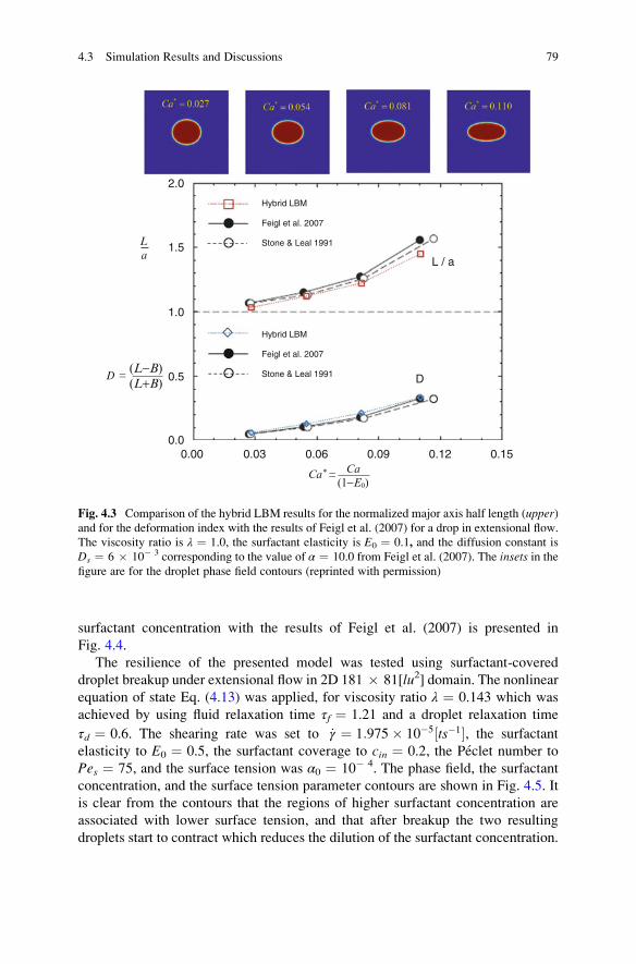
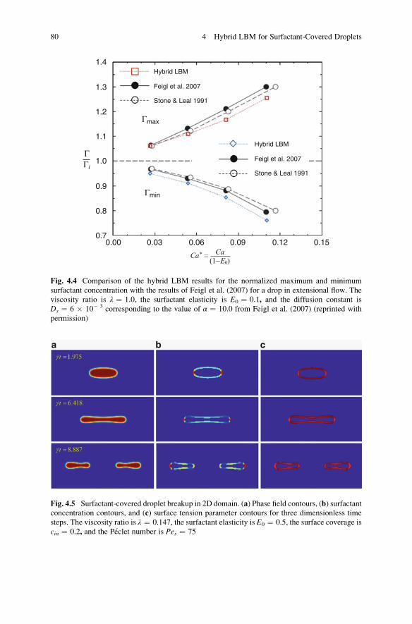
To validate the proposed algorithm, the results of the hybrid LBM for extensional

flow in 2D domain were compared with the numerical findings of Feigl

et al. (2007), who presented their results for the deformation index D ¼ (L � B)/(L + B), dimensionless major axis half length L/a, where a was the droplet radius

and B was the minor axis half length, and the dimensionless maximum and

minimum surfactant concentrations with respect to the equilibrium capillary

number Ca* ¼ Ca/(1 � E0). The surfactant elasticity was determined as

E0 ¼ Γ0RT/σ0 in which Γ0 was the initial concentration. The linear equation of

state was used with Γ* ¼ Γ/Γ0. The simulation was executed for one droplet under

extensional flow with viscosity ratio λ ¼ 1, surfactant elasticity E0 ¼ 0.1, and the

4.3 Simulation Results and Discussions 77



coefficient α ¼ Pes/Ca ¼ 10.0. To match the same conditions in the hybrid LBM

the surface tension parameter was set to α0 ¼ 10� 3, the initial surfactant concen-

tration to Γi ¼ 3 � 10� 4[lmol/lu2] and the diffusion constant to Ds ¼ 6 � 10� 3

[lu2ts� 1], for a range of capillary numbers 0.0243 � Ca � 0.099. The domain was

made of 123 � 123[lu2], the density was ρ ¼ 2.0[mu/lu2], and the relaxation time

was τ ¼ 1.0. The linear equation of state was used in this simulation. The results of

the presented model for the droplet deformation are presented in Fig. 4.3. A

comparison of the hybrid LBM results for the normalized maximum and minimum

Fig. 4.2 Flow chart for the hybrid LBM for surfactant-covered droplets


surfactant concentration with the results of Feigl et al. (2007) is presented in

Fig. 4.4.

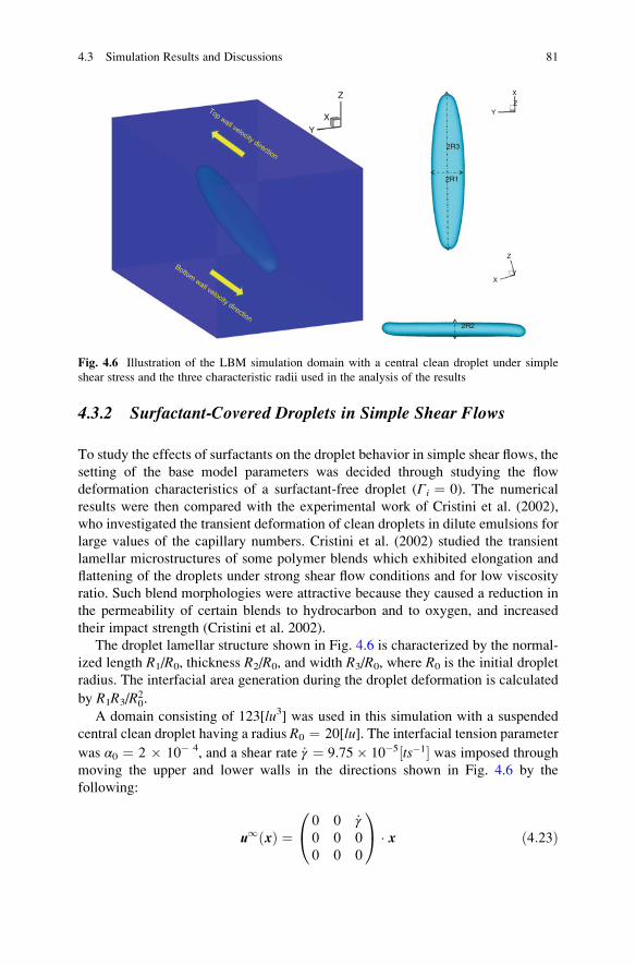
The resilience of the presented model was tested using surfactant-covered

droplet breakup under extensional flow in 2D 181 � 81[lu2] domain. The nonlinear

equation of state Eq. (4.13) was applied, for viscosity ratio λ ¼ 0.143 which was

achieved by using fluid relaxation time τf ¼ 1.21 and a droplet relaxation time

τd ¼ 0.6. The shearing rate was set to _γ ¼ 1:975� 10�5 ts�1½ �, the surfactant

elasticity to E0 ¼ 0.5, the surfactant coverage to cin ¼ 0.2, the Peclet number to

Pes ¼ 75, and the surface tension was α0 ¼ 10� 4. The phase field, the surfactant

concentration, and the surface tension parameter contours are shown in Fig. 4.5. It

is clear from the contours that the regions of higher surfactant concentration are

associated with lower surface tension, and that after breakup the two resulting

droplets start to contract which reduces the dilution of the surfactant concentration.

Hybrid LBM

Feigl et al. 2007

Stone & Leal 1991

0.12 0.150.090.060.030.000.0

0.5

1.0

1.5

2.0

L

Ca* Ca

D =

=

(L−B)(L+B)

(1−E0)

aL / a

D

Hybrid LBM

Feigl et al. 2007

Stone & Leal 1991

Fig. 4.3 Comparison of the hybrid LBM results for the normalized major axis half length (upper)and for the deformation index with the results of Feigl et al. (2007) for a drop in extensional flow.

The viscosity ratio is λ ¼ 1.0, the surfactant elasticity is E0 ¼ 0.1, and the diffusion constant is

Ds ¼ 6 � 10� 3 corresponding to the value of α ¼ 10.0 from Feigl et al. (2007). The insets in thefigure are for the droplet phase field contours (reprinted with permission)


1.4

1.3

1.2

1.1

1.0

0.9

0.8

0.70.00 0.03 0.06 0.09 0.12 0.15

Hybrid LBM

Feigl et al. 2007

Stone & Leal 1991

Hybrid LBM

Feigl et al. 2007

Stone & Leal 1991

Γmax

ΓΓi

Γmin

Ca* Ca=(1−E0)

Fig. 4.4 Comparison of the hybrid LBM results for the normalized maximum and minimum

surfactant concentration with the results of Feigl et al. (2007) for a drop in extensional flow. The

viscosity ratio is λ ¼ 1.0, the surfactant elasticity is E0 ¼ 0.1, and the diffusion constant is

Ds ¼ 6 � 10� 3 corresponding to the value of α ¼ 10.0 from Feigl et al. (2007) (reprinted with

permission)

Fig. 4.5 Surfactant-covered droplet breakup in 2D domain. (a) Phase field contours, (b) surfactant

concentration contours, and (c) surface tension parameter contours for three dimensionless time

steps. The viscosity ratio is λ ¼ 0.147, the surfactant elasticity is E0 ¼ 0.5, the surface coverage is

cin ¼ 0.2, and the Peclet number is Pes ¼ 75


4.3.2 Surfactant-Covered Droplets in Simple Shear Flows

To study the effects of surfactants on the droplet behavior in simple shear flows, the

setting of the base model parameters was decided through studying the flow

deformation characteristics of a surfactant-free droplet (Γi ¼ 0). The numerical

results were then compared with the experimental work of Cristini et al. (2002),

who investigated the transient deformation of clean droplets in dilute emulsions for

large values of the capillary numbers. Cristini et al. (2002) studied the transient

lamellar microstructures of some polymer blends which exhibited elongation and

flattening of the droplets under strong shear flow conditions and for low viscosity

ratio. Such blend morphologies were attractive because they caused a reduction in

the permeability of certain blends to hydrocarbon and to oxygen, and increased

their impact strength (Cristini et al. 2002).

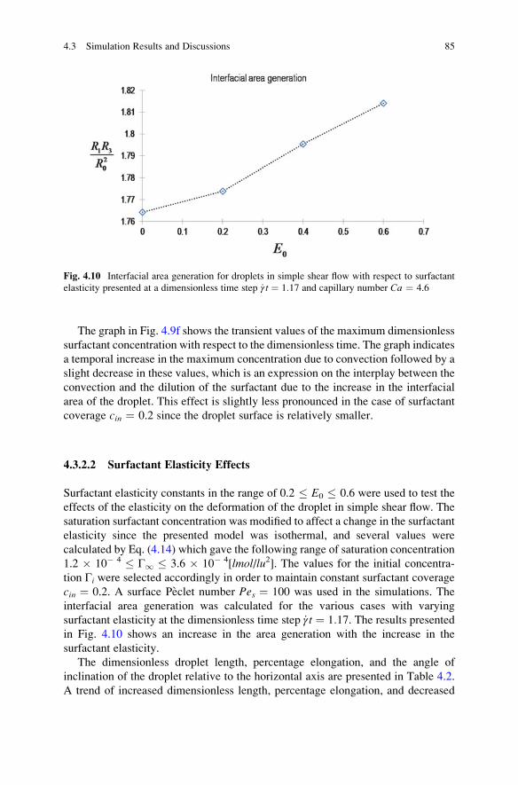
The droplet lamellar structure shown in Fig. 4.6 is characterized by the normal-

ized length R1/R0, thickness R2/R0, and width R3/R0, where R0 is the initial droplet

radius. The interfacial area generation during the droplet deformation is calculated

by R1R3/R20.

A domain consisting of 123[lu3] was used in this simulation with a suspended

central clean droplet having a radius R0 ¼ 20[lu]. The interfacial tension parameter

was α0 ¼ 2 � 10� 4, and a shear rate _γ ¼ 9:75� 10�5 ts�1½ � was imposed through

moving the upper and lower walls in the directions shown in Fig. 4.6 by the

following:

u1 xð Þ ¼0 0 _γ0 0 0

0 0 0

0@

1A � x ð4:23Þ

Z

2R3

2R1

2R2

X

ZY

Y

Z

X

XTop wall velocity direction

Bottom wall velocity direction

Y

Fig. 4.6 Illustration of the LBM simulation domain with a central clean droplet under simple

shear stress and the three characteristic radii used in the analysis of the results


The periodic boundary condition was used in all other directions. The relaxation

time for the ambient fluid was τm ¼ 1.213 and for the droplet τd ¼ 0.571 leading to

a viscosity ratio η ¼ 0.1. The interface viscosity was calculated by Eq. (2.15). The

density of both fluids was set to ρ ¼ 2[mu/lu3].The droplet deformation in simple shear flows is characterized by the capillary

number which is the ratio of the droplet deforming shear stress and the restoring

stress due to the interfacial tension:

Ca ¼ R0μm _γm

σ0ð4:24Þ

where σ0 is the interfacial tension of a clean droplet and μm is the dynamic viscosity

of the matrix. Equation (4.24) yielded a capillary number Ca ¼ 4.6 in correspon-

dence with one of the experimental condition of Cristini et al. (2002). The resulting

dimensionless width of the droplet from the presented model with respect to the

dimensionless time is shown in Fig. 4.7.

The clean droplet case showed a good agreement with the experimental data for

the dimensionless time _γ t � 2:0.Therefore the investigation of the area generation

due to the presence of surfactants will be limited to values of the dimensionless time

_γ t < 2:0 while other droplet flow deformation characteristics will be discussed for

time step _γ t ¼ 3:12 corresponding to the end of the simulation time which was

dictated by the desire of not allowing the droplet to deform beyond the periodic

boundaries.

Ca = 9.2

R3

R0

Ca = 4.6Ca = 2.3

1.1

1

0.9

0.80

LBM model

Cristini numerical

Cristini experimental

γ t1 2 3 4 5

⋅

Fig. 4.7 Comparison of the presented numerical model results with the experimental and numer-

ical results of Cristini et al. (2002) for a clean droplet dimensionless width as a function of the

dimensionless time. The viscosity ratio is λ ¼ 0.1, and the capillary number is Ca ¼ 4.6 (reprinted

with permission)



4.3.2.1 Surfactant Coverage Effects

To test the effects of surfactant coverage cin on the droplet deformation under

simple shear flow, the surfactant elasticity was set to E0 ¼ 0.2 as the use of this

value was justified by Velankar et al. (2002) for low-molecular-weight surfactants.

The saturation surfactant concentration was calculated using Eq. (4.14) and the

resulting value was Γ1 ¼ 1.2 � 10� 4[lmol/lu2]. This allowed the selection of the

various initial surfactant concentrations Γi in order to achieve the range of surfac-

tant coverage 0.2 � cin � 0.6. The surface Peclet number was set to Pes ¼ 10.

The interfacial area generation was calculated for the various cases at a dimen-

sionless time step _γ t ¼ 1:17corresponding to the greatest value for the ratioR3

R0which

was presented in Fig. 4.7. The results shown in Fig. 4.8 indicate an increase in the

area generation with the increase in the surfactant coverage as a consequence of the

simultaneous increase in the droplet elongation (R1), and flattening (R3).

The dimensionless length R1/R0, the percentage elongation increase relative to

the clean drop, and the reference angle θ� of the droplet inclination with respect to

the horizontal direction were calculated at dimensionless time step _γ t ¼ 3:12. Theresults presented in Table 4.1 imply that the greater the surfactant coverage the

Interfacial area generation

0

1.84

1.83

1.82

1.81

1.8

1.79

1.78

1.77

1.760.1 0.2 0.3 0.4 0.5 0.6 0.7

cin

R1R3

R02

Fig. 4.8 Interfacial area generation for droplets in simple shear flow with respect to initial

surfactant coverage presented at a dimensionless time step _γ t ¼ 1:17 and capillary number

Ca ¼ 4.6

Table 4.1 Transient dimensionless length, percentage elongation, and reference angle of incli-

nation measured in degrees, for the clean droplet and for the droplets with three initial values of

surfactant coverage cin at dimensionless time step _γ t ¼ 3:12

Cin R1/R0 % θ�

0 2.66 100.0 20.30

0.2 2.71 101.9 19.67

0.4 2.78 104.6 19.08

0.6 2.87 108.0 18.17


higher the values of the dimensionless length, the percentage elongation, and the

lower the angle of the droplet inclination.

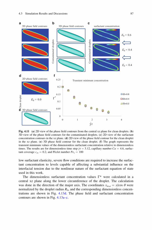
It is clear from the surfactant concentration contours in Fig. 4.9c (see Movie

C4.3.2.1—Surfshear) that the regions of higher surfactant concentration are located

around the tips of the droplet (see phase field density contours Fig. 4.9a and Movie

C4.3.2.1—3Dshear) in the directions of the walls velocities, as a consequence of the

convection of surfactants on the droplet interface. This also led to a greater droplet

deformation as this was evident from the results of Table 4.1.

The phase field contours for clean and contaminated droplets and the surfactant

concentration contours corresponding to the various values of the surfactant cov-

erage for dimensionless time _γ t ¼ 3:12 are presented in Fig. 4.9a–e.

a

d

e

b

f

c2D phase field contours 3D phase field contours

Transient maximum concentration0.7

0.6

0.5

0.4

0.3

0.2

0.10 1 2 3 4

Cin=0.6

Cin=0.4

Cin=0.2

surfactant concentration

2D phase field contours


Cle

an d

ropl

et

Con

tam

inat

ed d

ropl

ets

Con

tam

inat

ed d

ropl

ets

g t

cin = 0.6

cin = 0.4

cin = 0.2

cin = 0.0Γ*

⋅

Fig. 4.9 (a) 2D view of the phase field contours from the central xz plane for the contaminated

droplets. (b) 3D view of the phase field contours for the contaminated droplets surrounded by a

fictitious block to show the variance in their dimensions. (c) 2D xz plane view of the surfactant

concentration contours. (d) 2D xz plane view of the phase field contour for a clean drop. (e) 3D

view of the phase field contour for the clean drop. (f) Graph representing the transient maximum

values of the dimensionless surfactant concentration relative to dimensionless times. The results

are for dimensionless time step _γ t ¼ 3:12, capillary number Ca ¼ 4.6, surfactant elasticity

E0 ¼ 0.2, and Peclet number Pes ¼ 10


The graph in Fig. 4.9f shows the transient values of the maximum dimensionless

surfactant concentration with respect to the dimensionless time. The graph indicates

a temporal increase in the maximum concentration due to convection followed by a

slight decrease in these values, which is an expression on the interplay between the

convection and the dilution of the surfactant due to the increase in the interfacial

area of the droplet. This effect is slightly less pronounced in the case of surfactant

coverage cin ¼ 0.2 since the droplet surface is relatively smaller.

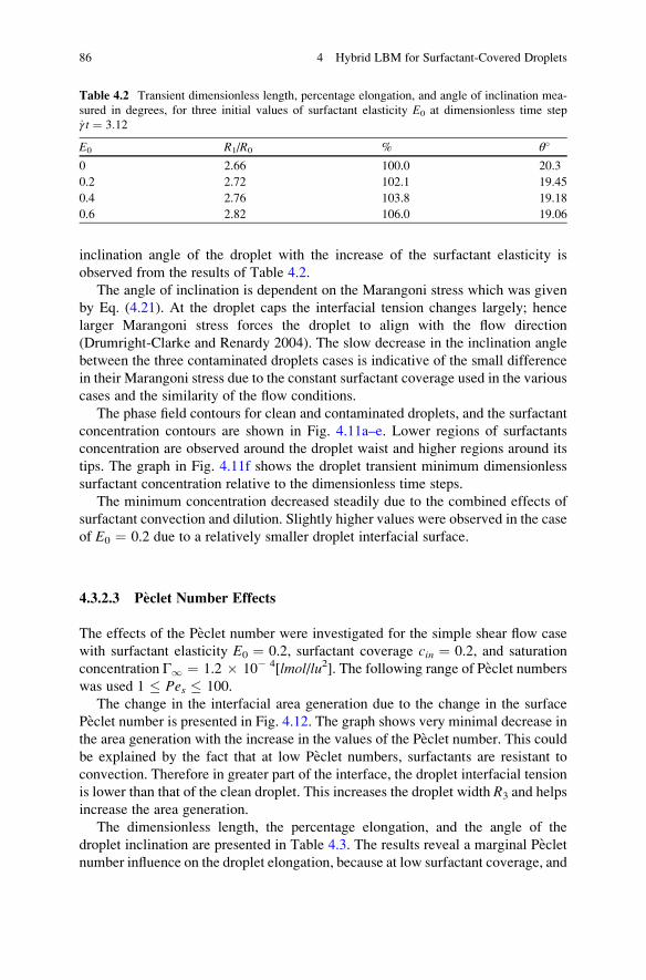
4.3.2.2 Surfactant Elasticity Effects

Surfactant elasticity constants in the range of 0.2 � E0 � 0.6 were used to test the

effects of the elasticity on the deformation of the droplet in simple shear flow. The

saturation surfactant concentration was modified to affect a change in the surfactant

elasticity since the presented model was isothermal, and several values were

calculated by Eq. (4.14) which gave the following range of saturation concentration

1.2 � 10� 4 � Γ1 � 3.6 � 10� 4[lmol/lu2]. The values for the initial concentra-

tion Γi were selected accordingly in order to maintain constant surfactant coverage

cin ¼ 0.2. A surface Peclet number Pes ¼ 100 was used in the simulations. The

interfacial area generation was calculated for the various cases with varying

surfactant elasticity at the dimensionless time step _γ t ¼ 1:17. The results presentedin Fig. 4.10 shows an increase in the area generation with the increase in the

surfactant elasticity.

The dimensionless droplet length, percentage elongation, and the angle of

inclination of the droplet relative to the horizontal axis are presented in Table 4.2.

A trend of increased dimensionless length, percentage elongation, and decreased

Fig. 4.10 Interfacial area generation for droplets in simple shear flow with respect to surfactant

elasticity presented at a dimensionless time step _γ t ¼ 1:17 and capillary number Ca ¼ 4.6


inclination angle of the droplet with the increase of the surfactant elasticity is

observed from the results of Table 4.2.

The angle of inclination is dependent on the Marangoni stress which was given

by Eq. (4.21). At the droplet caps the interfacial tension changes largely; hence

larger Marangoni stress forces the droplet to align with the flow direction

(Drumright-Clarke and Renardy 2004). The slow decrease in the inclination angle

between the three contaminated droplets cases is indicative of the small difference

in their Marangoni stress due to the constant surfactant coverage used in the various

cases and the similarity of the flow conditions.

The phase field contours for clean and contaminated droplets, and the surfactant

concentration contours are shown in Fig. 4.11a–e. Lower regions of surfactants

concentration are observed around the droplet waist and higher regions around its

tips. The graph in Fig. 4.11f shows the droplet transient minimum dimensionless

surfactant concentration relative to the dimensionless time steps.

The minimum concentration decreased steadily due to the combined effects of

surfactant convection and dilution. Slightly higher values were observed in the case

of E0 ¼ 0.2 due to a relatively smaller droplet interfacial surface.

4.3.2.3 Peclet Number Effects

The effects of the Peclet number were investigated for the simple shear flow case

with surfactant elasticity E0 ¼ 0.2, surfactant coverage cin ¼ 0.2, and saturation

concentration Γ1 ¼ 1.2 � 10� 4[lmol/lu2]. The following range of Peclet numbers

was used 1 � Pes � 100.

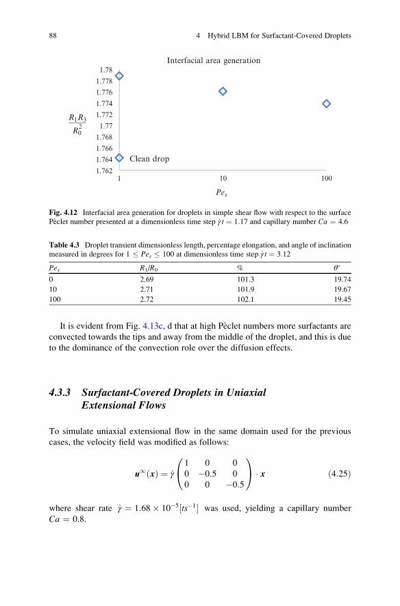
The change in the interfacial area generation due to the change in the surface

Peclet number is presented in Fig. 4.12. The graph shows very minimal decrease in

the area generation with the increase in the values of the Peclet number. This could

be explained by the fact that at low Peclet numbers, surfactants are resistant to

convection. Therefore in greater part of the interface, the droplet interfacial tension

is lower than that of the clean droplet. This increases the droplet width R3 and helps

increase the area generation.

The dimensionless length, the percentage elongation, and the angle of the

droplet inclination are presented in Table 4.3. The results reveal a marginal Peclet

number influence on the droplet elongation, because at low surfactant coverage, and

Table 4.2 Transient dimensionless length, percentage elongation, and angle of inclination mea-

sured in degrees, for three initial values of surfactant elasticity E0 at dimensionless time step

_γ t ¼ 3:12

E0 R1/R0 % θ�

0 2.66 100.0 20.3

0.2 2.72 102.1 19.45

0.4 2.76 103.8 19.18

0.6 2.82 106.0 19.06


low surfactant elasticity, severe flow conditions are required to increase the surfac-

tant concentration to levels capable of affecting a substantial influence on the

interfacial tension due to the nonlinear nature of the surfactant equation of state

used in this work.

The dimensionless surfactant concentration values Γ* were calculated in a

central xz plane along the lower circumference of the droplet. The calculation

was done in the direction of the major axis. The coordinates xm,a ¼ x/cos θ were

normalized by the droplet radius R0, and the corresponding dimensionless concen-

trations are shown in Fig. 4.13d. The phase field and surfactant concentration

contours are shown in Fig. 4.13a–c.

a

d

e

f

b c2D phase field contours 3D phase field contours surfactant concentration



Cle

an d

ropl

et

Con

tam

inat

ed d

ropl

ets

Con

tam

inat

ed d

ropl

ets

Transient minimum concentration0.25

0.2

0.15

0.1

0.05

0

0 1 2 3 4

E0 = 0.6

E0 = 0.4

E0 = 0.4

Γ*E0=0.6

E0=0.4

E0=0.2

E0 = 0.0

g t⋅

Fig. 4.11 (a) 2D view of the phase field contours from the central xz plane for clean droplets. (b)

3D view of the phase field contours for the contaminated droplets. (c) 2D view of the surfactant

concentration contours in the xz plane. (d) 2D view of the phase field contour for the clean droplet

in the xz plane. (e) 3D phase field contour for the clean droplet. (f) The graph represents the

transient minimum values of the dimensionless surfactant concentration relative to dimensionless

times. The results are for dimensionless time step _γ t ¼ 3:12, capillary number Ca ¼ 4.6, surfac-

tant coverage cin ¼ 0.2, and Peclet number Pes ¼ 100


It is evident from Fig. 4.13c, d that at high Peclet numbers more surfactants are

convected towards the tips and away from the middle of the droplet, and this is due

to the dominance of the convection role over the diffusion effects.

4.3.3 Surfactant-Covered Droplets in UniaxialExtensional Flows

To simulate uniaxial extensional flow in the same domain used for the previous

cases, the velocity field was modified as follows:

u1 xð Þ ¼ _γ1 0 0

0 �0:5 0

0 0 �0:5

0@

1A � x ð4:25Þ

where shear rate _γ ¼ 1:68� 10�5 ts�1½ � was used, yielding a capillary number

Ca ¼ 0.8.

Interfacial area generation

Clean drop

1.78

1.778

1.776

1.774

1.772

1.77

1.768

1.766

1.764

1.7621 10 100

R1R3

Pes

R02

Fig. 4.12 Interfacial area generation for droplets in simple shear flow with respect to the surface

Peclet number presented at a dimensionless time step _γ t ¼ 1:17 and capillary number Ca ¼ 4.6

Table 4.3 Droplet transient dimensionless length, percentage elongation, and angle of inclination

measured in degrees for 1 � Pes � 100 at dimensionless time step _γ t ¼ 3:12

Pes R1/R0 % θ�

0 2.69 101.3 19.74

10 2.71 101.9 19.67

100 2.72 102.1 19.45


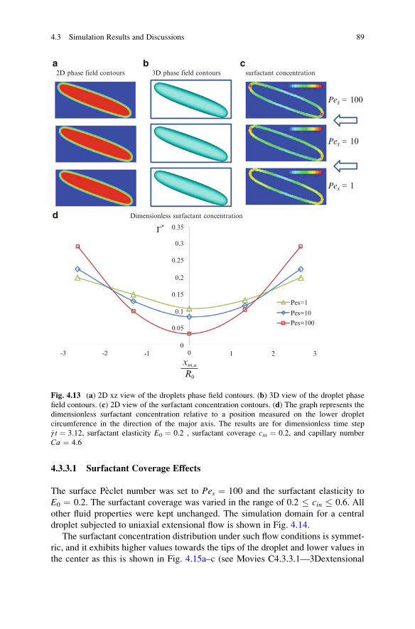
4.3.3.1 Surfactant Coverage Effects

The surface Peclet number was set to Pes ¼ 100 and the surfactant elasticity to

E0 ¼ 0.2. The surfactant coverage was varied in the range of 0.2 � cin � 0.6. All

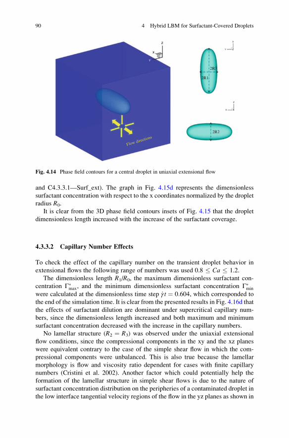
other fluid properties were kept unchanged. The simulation domain for a central

droplet subjected to uniaxial extensional flow is shown in Fig. 4.14.

The surfactant concentration distribution under such flow conditions is symmet-

ric, and it exhibits higher values towards the tips of the droplet and lower values in

the center as this is shown in Fig. 4.15a–c (see Movies C4.3.3.1—3Dextensional

a

d

b c2D phase field contours 3D phase field contours

Dimensionless surfactant concentration

surfactant concentration

Pes = 100

Pes = 10

Pes = 1

Γ* 0.35

0.3

0.25

0.2

0.15

0.1

0.05

0-3 -2 -1 0 1 2 3

Pes=1

Pes=10

Pes=100

xm,a

R0

Fig. 4.13 (a) 2D xz view of the droplets phase field contours. (b) 3D view of the droplet phase

field contours. (c) 2D view of the surfactant concentration contours. (d) The graph represents the

dimensionless surfactant concentration relative to a position measured on the lower droplet

circumference in the direction of the major axis. The results are for dimensionless time step

_γ t ¼ 3:12, surfactant elasticity E0 ¼ 0.2 , surfactant coverage cin ¼ 0.2, and capillary number

Ca ¼ 4.6


and C4.3.3.1—Surf_ext). The graph in Fig. 4.15d represents the dimensionless

surfactant concentration with respect to the x coordinates normalized by the droplet

radius R0.

It is clear from the 3D phase field contours insets of Fig. 4.15 that the droplet

dimensionless length increased with the increase of the surfactant coverage.

4.3.3.2 Capillary Number Effects

To check the effect of the capillary number on the transient droplet behavior in

extensional flows the following range of numbers was used 0.8 � Ca � 1.2.

The dimensionless length R1/R0, the maximum dimensionless surfactant con-

centration Γ�max, and the minimum dimensionless surfactant concentration Γ�

min

were calculated at the dimensionless time step _γ t ¼ 0:604, which corresponded to

the end of the simulation time. It is clear from the presented results in Fig. 4.16d that

the effects of surfactant dilution are dominant under supercritical capillary num-

bers, since the dimensionless length increased and both maximum and minimum

surfactant concentration decreased with the increase in the capillary numbers.

No lamellar structure (R2 ¼ R3) was observed under the uniaxial extensional

flow conditions, since the compressional components in the xy and the xz planes

were equivalent contrary to the case of the simple shear flow in which the com-

pressional components were unbalanced. This is also true because the lamellar

morphology is flow and viscosity ratio dependent for cases with finite capillary

numbers (Cristini et al. 2002). Another factor which could potentially help the

formation of the lamellar structure in simple shear flows is due to the nature of

surfactant concentration distribution on the peripheries of a contaminated droplet in

the low interface tangential velocity regions of the flow in the yz planes as shown in

z

x

Flow directions

2R3

2R1

2R2

Y

Y

Y

Z

Z

X

X

Fig. 4.14 Phase field contours for a central droplet in uniaxial extensional flow


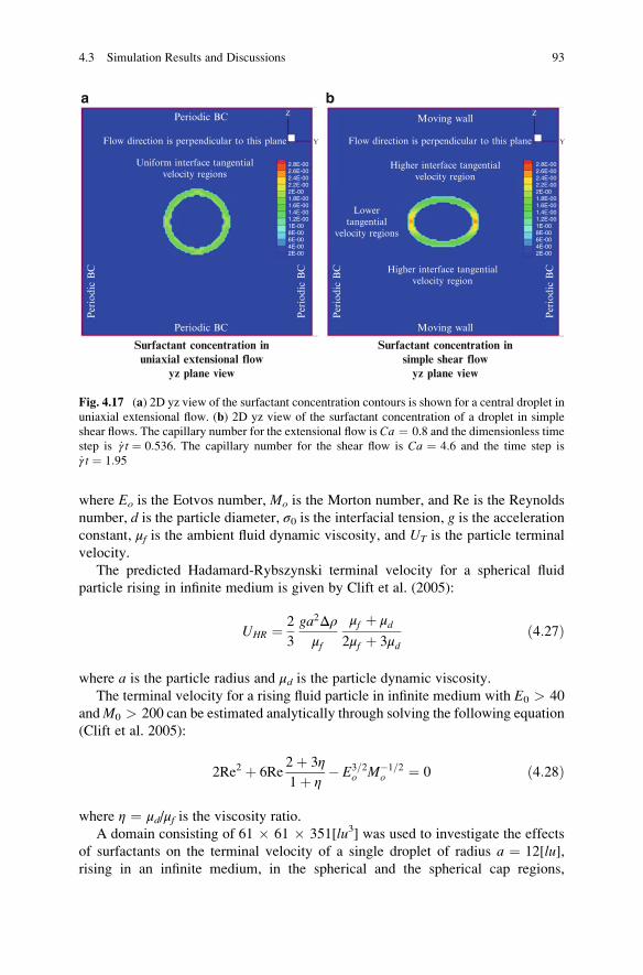
Fig. 4.17b. These regions are characterized by lower convection effects leading to

higher local surfactant concentrations which act to reduce the droplet interfacial

tension, hence locally lowering its capillary number and making it more deform-

able. This does not occur in the uniaxial extensional flow due to its uniform

tangential velocity profile in the indicated region of Fig. 4.17a.

4.3.4 Buoyancy of Surfactant-Covered Dropletsin Infinite Medium

The effect of surfactants on buoyant droplets and bubbles named here as fluid

particles was studied both experimentally (Almatroushi and Borhan 2004; Griffith

1962; Bel Fdhila and Duineveld 1996; Alves et al. 2005) and numerically

a

d

b

Cin=0.2

Cin=0.4

Cin=0.6

c

Dimensionless surfactant concentration

-3 -2 -1 0

0

0.1

0.2

0.3

0.4

0.5

0.6

0.7

0.8

0.9

1 2 3

Γ*

cin = 0.4 cin = 0.6cin = 0.2

R1/R0 = 2.18

R1/R0 = 2.08

R1/R0 = 1.98

x

R0

Fig. 4.15 (a–c) 2D xz view of the surfactant concentration contours for a central droplet in

uniaxial extensional flow, for three values of the surfactant coverage. (d) Graph representing the

dimensionless surfactant concentration in the xz plane as a function of the horizontal coordinate

normalized by the droplet radius for _γ t ¼ 0:604, Ca ¼ 0.8, Pes ¼ 100, and E0 ¼ 0.2. The insets inthe graph are for the 3D view of the phase field contours


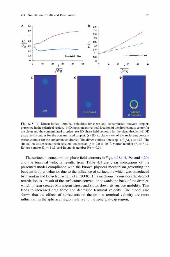
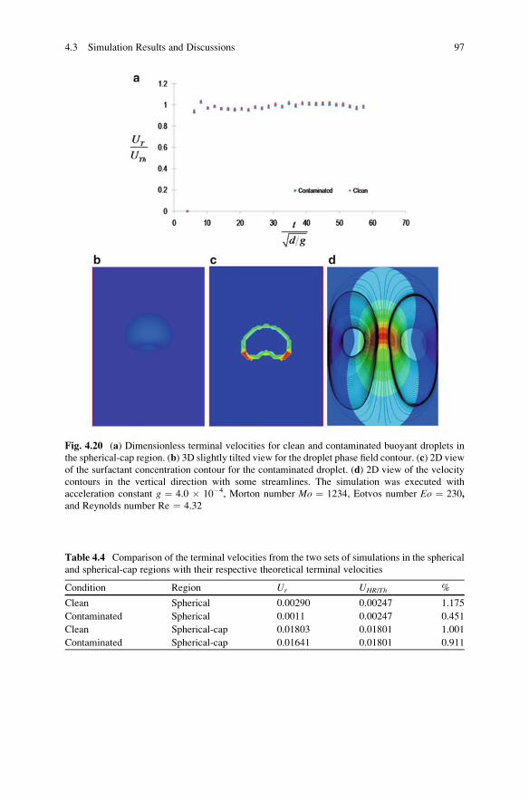
(Bel Fdhila and Duineveld 1996; Tasoglu et al. 2008). It was found that surfactants

generally reduce significantly the particle’s terminal velocity below the classical

Hadamard-Rybszynski prediction in the spherical region of the shape regime;

however in other shape regions the particle retardation due to surfactants is less

effective (Tasoglu et al. 2008).

Buoyancy-driven fluid particles are characterized by the following dimension-

less numbers:

Eo ¼ gΔρd2

σ0,Mo ¼

gμ4fΔρρ2f σ0

3, Re ¼ UTdρf

μfð4:26Þ

Fig. 4.16 (a–c) 2D view of the surfactant concentration contours on droplets in uniaxial exten-

sional flow for a range of capillary number 08 � Ca � 1.2. (d) Graph representing the values of

the droplet dimensionless R1/R0, the dimensionless maximum Γ�max, and minimum Γ�

min surfactant

concentration, respectively at dimensionless time step _γ t ¼ 0:604. The insets in the graph are for

the 3D view phase field contours


where Eo is the Eotvos number, Mo is the Morton number, and Re is the Reynolds

number, d is the particle diameter, σ0 is the interfacial tension, g is the accelerationconstant, μf is the ambient fluid dynamic viscosity, and UT is the particle terminal

velocity.

The predicted Hadamard-Rybszynski terminal velocity for a spherical fluid

particle rising in infinite medium is given by Clift et al. (2005):

UHR ¼ 2

3

ga2Δρμf

μf þ μd2μf þ 3μd

ð4:27Þ

where a is the particle radius and μd is the particle dynamic viscosity.

The terminal velocity for a rising fluid particle in infinite medium with E0 > 40

andM0 > 200 can be estimated analytically through solving the following equation

(Clift et al. 2005):

2Re2 þ 6Re2þ 3η

1þ η� E3=2

o M�1=2o ¼ 0 ð4:28Þ

where η ¼ μd/μf is the viscosity ratio.

A domain consisting of 61 � 61 � 351[lu3] was used to investigate the effects

of surfactants on the terminal velocity of a single droplet of radius a ¼ 12[lu],rising in an infinite medium, in the spherical and the spherical cap regions,

aPeriodic BC

Periodic BC

Per

iodi

c B

C

Per

iodi

c B

C

Per

iodi

c B

C

Moving wall

Moving wall

Lowertangential

velocity regions

Higher interface tangentialvelocity region

Higher interface tangentialvelocity region

Uniform interface tangentialvelocity regions

Flow direction is perpendicular to this planeFlow direction is perpendicular to this plane

Z

Y

Z

Y

Per

iodi

c B

C

Surfactant concentration inuniaxial extensional flow

yz plane view

Surfactant concentration insimple shear flow

yz plane view

b

2E-004E-006E-008E-001E-001.2E-001.4E-001.6E-001.8E-00

2.2E-002.4E-002.6E-002.8E-00

2E-00

2E-004E-006E-008E-001E-001.2E-001.4E-001.6E-001.8E-00

2.2E-002.4E-002.6E-002.8E-00

2E-00

Fig. 4.17 (a) 2D yz view of the surfactant concentration contours is shown for a central droplet in

uniaxial extensional flow. (b) 2D yz view of the surfactant concentration of a droplet in simple

shear flows. The capillary number for the extensional flow is Ca ¼ 0.8 and the dimensionless time

step is _γ t ¼ 0:536. The capillary number for the shear flow is Ca ¼ 4.6 and the time step is

_γ t ¼ 1:95


respectively. The density of the suspending fluid was ρf ¼ 2[mu/lu3], and the

droplet density was ρd ¼ 1.0[mu/lu3]. The relaxation time was set to τ ¼ 1.0

leading to dynamic viscosities μf ¼ 0.333 and μd ¼ 0.1666 for the surrounding

fluid and the droplet, respectively. The periodic condition was applied in all

directions. The interfacial tension was set to σ0 ¼ 10� 3.

Two set of simulations were executed in this section, in which the acceleration

constants were varied to produce the two required shapes. In each set of simula-

tions the clean and the contaminated droplet terminal velocities were calculated

and measured consecutively. The contaminated droplets cases had their surfactant

elasticity set to E0 ¼ 0.5 leading to a saturation surfactant concentration

Γ1 ¼ 1.5 � 10� 3 and the surfactant coverage was set to cin ¼ 0.4. The Peclet

number was set to Pes ¼ 40 and the diffusion coefficient was evaluated based on

the following relation:

Pes ¼ UT‘

Dsð4:29Þ

where UT is the terminal velocity, ‘ is the vertical distance required for the clean

droplet to attain its terminal velocity.

The resulting terminal velocities of the clean and the contaminated

buoyant droplets in the spherical shape region were due to acceleration constant

g ¼ 2.0 � 10�5[lu/ts�2] which led to Morton number Mo ¼ 61.7, Eotvos number

Eo ¼ 11.5, and Reynolds number Re ¼ 0.34. The normalized terminal velocities

by the Hadamard-Rybszynski terminal velocity UHR and the normalized mass

center vertical locations by the domain length L calculated with respect to normal-

ized time byffiffiffiffiffiffiffiffid=g

pare shown in Fig. 4.18.

The terminal velocities of the clean and contaminated buoyant droplets

in the spherical-cap shape region were produced by acceleration constant

g ¼ 2.0 � 10�4[lu/ts�2] which yielded Morton number Mo ¼ 617, Eotvos

number Eo ¼ 115, and Reynolds number Re ¼ 2.6. The normalized terminal

velocities by the theoretical droplet terminal velocity UTh and the normalized

mass center vertical locations by the domain length L calculated with respect

to normalized time byffiffiffiffiffiffiffiffid=g

pare shown in Fig. 4.19.

A third simulation was executed using the parameters from the second case with

g ¼ 4.0 � 10�4[lu/ts�2] and the results for the phase field, the surfactant concen-

tration distribution, and velocity contours are shown in Fig. 4.20. The increase in

the acceleration resulted in Morton numberMo ¼ 1234, Eotvos number Eo ¼ 230,

and Reynolds number Re ¼ 4.32. Under such condition higher droplet deformation

and very marginal effects of surfactant retardation are witnessed.

The results for the terminal velocities and their ratio with respect to the theoret-

ical values calculated by Eqs. (4.27) and (4.28) from both set of simulations are

summarized in Table 4.4.


The surfactant concentration phase field contours in Figs. 4.18e, 4.19e, and 4.20c

and the terminal velocity results from Table 4.4 are clear indications of the

presented model compliance with the known physical mechanism governing the

buoyant droplet behavior due to the influence of surfactants which was introduced

by Frumkin and Levich (Tasoglu et al. 2008). This mechanism considers the droplet

retardation as a result of the surfactants convection towards the back of the droplet,

which in turn creates Marangoni stress and slows down its surface mobility. This

leads to increased drag force and decreased terminal velocity. The model also

shows that the effects of surfactants on the droplet terminal velocity are more

influential in the spherical region relative to the spherical-cap region.

Fig. 4.18 (a) Dimensionless terminal velocities for clean and contaminated buoyant droplets

presented in the spherical region. (b) Dimensionless vertical location of the droplet mass center for

the clean and the contaminated droplets. (c) 3D phase field contours for the clean droplet, (d) 3D

phase field contour for the contaminated droplet. (e) 2D xz plane view of the surfactant concen-

tration contour for the contaminated droplet. The dimensionless time step is t=ffiffiffiffiffiffiffiffid=g

p ¼ 43:3. Thesimulation was executed with acceleration constant g ¼ 2.0 � 10�5, Morton number Mo ¼ 61.7,

Eotvos number Eo ¼ 11.5, and Reynolds number Re ¼ 0.34


Fig. 4.19 (a) Dimensionless terminal velocities for clean and contaminated buoyant droplets

presented in the spherical-cap region. (b) Dimensionless vertical location of the droplet mass

center for the clean and the contaminated droplets. (c) 3D phase field contours for the clean

droplet. (d) 3D phase field contour for the contaminated droplet. (e) 2D view of the surfactant

concentration contour for the contaminated droplet. The dimensionless time step is

t=ffiffiffiffiffiffiffiffid=g

p ¼ 49:07. The simulation was executed with acceleration constant g ¼ 2.0 � 10�4,

Morton number Mo ¼ 617, Eotvos number Eo ¼ 115, and Reynolds number Re ¼ 2.6


Fig. 4.20 (a) Dimensionless terminal velocities for clean and contaminated buoyant droplets in

the spherical-cap region. (b) 3D slightly tilted view for the droplet phase field contour. (c) 2D view

of the surfactant concentration contour for the contaminated droplet. (d) 2D view of the velocity

contours in the vertical direction with some streamlines. The simulation was executed with

acceleration constant g ¼ 4.0 � 10�4, Morton number Mo ¼ 1234, Eotvos number Eo ¼ 230,

and Reynolds number Re ¼ 4.32

Table 4.4 Comparison of the terminal velocities from the two sets of simulations in the spherical

and spherical-cap regions with their respective theoretical terminal velocities

Condition Region Ur UHR/Th %

Clean Spherical 0.00290 0.00247 1.175

Contaminated Spherical 0.0011 0.00247 0.451

Clean Spherical-cap 0.01803 0.01801 1.001

Contaminated Spherical-cap 0.01641 0.01801 0.911


Date post:	25-Dec-2016
Category:	Documents
Upload:	sasidhar
View:	214 times
Download:	1 times

Accelerated Lattice Boltzmann Model for Colloidal Suspensions || Hybrid LBM for Surfactant-Covered...

Documents