{nikunj, nico, lin}@cs.unc.eduDepartment of Computer Science
UNC Chapel Hill
Abstract
We present an efficient technique to model sound propagation accu-rately in an arbitrary 3D scene by numerically integrating the waveequation. We show that by performing an offline modal analysisand using eigenvalues from a refined mesh, we can simulate soundpropagation with reduced dispersion on a much coarser mesh, en-abling accelerated computation. Since performing a modal analysison the complete scene is usually not feasible, we present a domaindecomposition approach to drastically shorten the pre-processingtime. We introduce a simple, efficient and stable technique for han-dling the communication between the domain partitions. We vali-date the accuracy of our approach against cases with known analyt-ical solutions. With our approach, we have observed up to an or-der of magnitude speedup compared to a standard finite-differencetechnique.
CR Categories: H.5.5 [Information Interfaces and Presenta-tion]: Sound and Music Computing—Modeling, Methodologiesand techniques I.3.5 [Computer Graphics]: Computational Ge-ometry and Object Modeling—Physically based modeling I.3.7[Computer Graphics]: Three-Dimensional Graphics and Realism—Animation
One of the most important considerations in architectural design isroom acoustics and noise control. Computer-aided tools are indis-pensable for evaluating the acoustic properties of a proposed audi-torium layout or determining the noise level of any machinery ona factory floor. Furthermore, the acoustics of a virtual scene canalso affect the sense of immersion in the simulated environment.Acoustic modeling can provide sound cues to a user’s navigation,communication, and exploration of a virtual environment.
Humans have a very acute sense for reverberations and other acous-tical effects and these tend to convey a sense of the geometric qual-ities of the scene to the listener. For example, delayed, unatten-uated echoes tend to convey the impression of a big hall. Dueto the sound propagation and the enhanced immersion achievablewith correct acoustics, the problem of modeling sound propaga-tion accurately and efficiently has traditionally been an active areaof research. A few characteristics pertinent to sound waves makemodeling sound propagation a challenging problem. First of all,audible sound has wavelength in the range of a few millimeters to a
Figure 1: Efficient sound propagation simulation in an architec-tural model. We demonstrate our algorithm on a modestly complex3D environment, enabling realistic interference, diffraction and re-verberation sound effects. The volume of this scene is ≈ 500m3,which was partitioned into 290 arbitrary partitions with near-equalvolume. The bottom of the figure shows the partitioning on a hor-izontal 2D slice of the scene, taken about 1 meter above ground.Black indicates walls and the free-space partitions are color-codedwith different colors. We are able to generate one sample of audioon this scene in about 250 ms.
few meters, which is comparable to most objects’ dimensions andthus capturing diffraction accurately is very important, especiallyfor low frequencies. Secondly, sound waves are coherent, whichmeans that two sound waves must be added taking their phases intoaccount. Therefore, capturing interference is critical for modelingsound propagation accurately. Thirdly, a full time-domain solutionis needed (as opposed to only a steady-state solution as in globalillumination), at sampling rates in the Kilohertz (kHz) range fordynamic sound sources and listener.
Prior research in sound propagation modeling falls broadly into twocategories: geometric methods based on a ray/beam approximationof sound and numerical methods that seek to solve the underlyingwave-equation for sound propagation directly on a discretization ofthe domain. The problem with geometric methods is that they of-ten assume little diffraction and capturing it accurately in such aframework is quite difficult. Also, capturing higher-order reflec-tions using such schemes is difficult due to the large number ofpropagation paths that must be computed. Numerical methods, incontrast, elegantly capture all wave phenomena, including higher-order reflections in a single framework. However, they are compu-tationally expensive, especially for high frequencies, as the numberof elements depends cubically on the diameter of the scene beingmodeled, in 3D.
Main Results: In this paper, we propose a technique based on theFinite Difference Method (FDM) and modal analysis, which is ca-
91
pable of performing accurate sound propagation simulation for ar-bitrary static 3D scenes with frequencies up to 1 kHz. The sourcesand the listener may move arbitrarily through the scene. The mainidea behind our approach is that the wave-equation on a domaincan be integrated exactly in time once space has been discretized,by performing modal analysis, which involves computing an offlinematrix diagonalization. However, as we describe later, the pre-processing for this basic approach is computationally intractableboth in terms of time and memory consumption, especially in 3Dfor high-resolution meshes which are required for realistic simula-tion of frequencies in the kHz range.
In order to remedy this problem and improve the runtime efficiency,we introduce two acceleration techniques –
1. A domain decomposition technique in which the domain is di-vided into many non-overlapping partitions and modal anal-ysis on each partition is performed separately. This makespre-processing computationally tractable, as it is typically in-feasible in 3D to carry out a modal analysis on the completescene. At runtime, the sound is simulated within each parti-tion using a modal technique described later and an explicitcommunication step is performed at the partition interfaces ateach time-step. We discuss a simple second-order integrationscheme for performing the communication, that is both effi-cient and stable.
2. An eigenvalue correction technique that utilizes correctedeigenvalues precomputed using modal analysis on a refinedmesh and enables accelerated sound propagation simulationon a coarser mesh at runtime, without much loss of accu-racy. This technique incurs no additional runtime overheadand simply offers a trade-off between accuracy at runtime andslightly increased pre-processing time. We discuss how to findthe best trade-off for a given scene later in the paper. With thistechnique we are able to perform reasonably accurate acous-tic simulations on a mesh with only about 2-4 spatial samplesper the smallest simulated wavelength, instead of 8-10 sam-ples, as usually used in numerical simulations [Alford et al.1974].
As we describe later, together, these two techniques offer up toan order of magnitude improvement in terms of runtime efficiencyover a standard numerical approach, enabling realistic sound simu-lation on moderately large scenes in 3D.
The main characteristics of our approach are:
• Automatic capturing of all wave phenomena, includingdiffraction and reflection, in one unified framework;
• Ability to perform simulations on very coarse meshes whileretaining good accuracy, resulting in large reduction in com-putational requirements;
• Simple domain decomposition technique for handling largescenes.
Organization: The rest of the paper is organized as follows. Wereview related work in Section 2. We present the problem formu-lation for modeling sound propagation in 3D scenes along with theefficiency considerations in Section 3. We then describe our eigen-value correction and domain decomposition techniques that enableefficient sound propagation, in Section 4. In Section 5, we discussimplementation issues and demonstrate the results of our systemon moderately complex scenes, along with the validation of its ac-curacy and efficiency. Finally, we conclude with possible futureresearch directions.
2 Previous Work
Room acoustics has been an active area of research for more thanfive decades [Sabine 1953]. Depending on the amount of computerequired and achievable accuracy, methods for simulating soundpropagation can be broadly classified into two categories: Geomet-ric and Numerical methods. In the following, we will discuss thesemethods in detail. For a basic treatment of the theory and practice ofroom acoustics, the reader is referred to the classic texts [Kuttruff2000; Kinsler et al. 1999]. For a recent survey of computationalacoustics, please refer to [Lokki 2002].
2.1 Geometric Methods
Geometric methods assume that sound propagates in straight linesunless obstructed by an object, much like light. However, this ap-proximation works well only when the wavelength of the soundis much smaller than the size of the objects in the scene, so thatdiffraction can be effectively neglected. Nevertheless, owing totheir simplicity and efficiency, geometric techniques were the firstto be formulated and implemented on a digital computer [Krock-stadt 1968; Allen and Berkley 1979]. Over the decades, there hasbeen a significant amount of research on geometric methods, whichonly differ from each other in the way sound propagation is approx-imated. Some salient examples are, the image source method [Allenand Berkley 1979], ray-tracing [Krockstadt 1968], beam-tracing[Min and Funkhouser 2000; Tsingos et al. 2001; Funkhouser et al.2003; Funkhouser et al. 2004; Antonacci et al. 2004], or phonon-tracing [Bertram et al. 2005; Deines et al. 2006].
2.2 Numerical Methods
In contrast to geometric methods, numerical methods typicallysolve for the complete sound field by numerically evaluating thewave equation after suitable discretization. Since the completefield is resolved at each time-step, these methods typically scalepoorly as the size of the scene is increased. However, the strengthof numerical methods is that they are very accurate, especially forlow frequencies in the range of a few hundred Hertz, which havewavelengths in the range of meters and exhibit noticeable diffrac-tion. Geometric methods, by their basic assumption, do not cap-ture such effects. Although there have been attempts to accountfor diffraction using the Geometric Theory for Diffraction [Tsingoset al. 2001], integrating accurate diffraction effects in a geometricsolver still remains a challenging problem. Based on the choiceof discretization, numerical methods for acoustics may be roughlyclassified into: Finite Element Method (FEM), Boundary ElementMethod (BEM), Digital Waveguide Mesh (DWM) and Finite Dif-ference Time Domain (FDTD) Method.
FEM/BEM is typically used to find the frequency-domain (in otherwords, steady state) response of an environment only, as opposedto the full time-domain response [Kleiner et al. 1993]. DWM wasintroduced by Duyne [Van Duyne and Smith 1993] as a methodto perform efficient time-domain simulation of wave propagation.The basic idea is to model the medium as a mesh of 1D waveg-uides, which carry waves along them as per the 1D wave equa-tion, for which the analytical solution is known. The nodes in themesh where these waveguides intersect are implemented as scatter-ing junctions which ensure that the incoming and outgoing acousticenergy at each junction is distributed properly. Since its introduc-tion, DWM has been an active area of research for room acous-tics [Savioja et al. 1994; Savioja et al. 1995; Karjalainen and Erkut2004]. For a brief survey of different methods for room acousticsand an introduction to DWM in this context, the reader is referred
92
to [Savioja 1999]. And, for a very recent survey on the state of theart in DWM, please refer to [Murphy et al. 2007].
The FDTD method was first introduced to room acoustics in [Bot-teldooren 1994; Botteldooren 1995] and is most closely related toour work. A typical FDTD scheme begins by first subdividing thedomain into a grid. In most cases, as in this paper, the grid is carte-sian with uniform cell size. Next, the continuum spatial operatorsare approximated by their discrete representation. At each time-step, the whole sound field in each cell is updated based on the fieldvalues at the previous time-step(s). Different FDTD schemes differin the way the spatial operator is approximated and the rules thatare used to update the field values. FDTD for acoustics has been avery active area of research, especially for low-frequency acousticsimulation on small rooms [Sakamoto et al. 2004; Sakamoto et al.2006]. Although DWM and FDTD appear quite different, they areactually equivalent [Van Duyne and Smith 1993]. In fact, not onlyare they equivalent, one can mix the two within the same domain[Karjalainen and Erkut 2004].
However, both DWM and FDTD face the same computational chal-lenges: For medium-range frequencies in the range of a Kilohertzand/or large architectural scenes, the compute requirements growsuper-linearly in higher dimensions and thus quickly become in-tractable, as both methods require a fine mesh to resolve the small-est wavelength. In this paper, we present a technique which is ableto perform acoustic simulation on a very coarse mesh, thereby re-ducing the computational requirements, at the cost of a slight lossin accuracy. This is done by first dividing the domain into manynon-overlapping partitions and then performing modal analysis oneach separately.
Modal analysis is a very well-known technique and it would benearly impossible to mention all the branches of science where ithas been applied. However, an area of research close to this workwhere modal analysis has found a lot of application is physically-based sound synthesis [van den Doel et al. 2001; O’Brien et al.2002; Raghuvanshi and Lin 2006]. For sound synthesis, modalanalysis is typically performed to find the vibrational modes of anelastic object and a complex vibration expressed as a linear combi-nation of these modes. Analogously for acoustics, modal analysisyields the resonant modes of pressure vibrations in a room, and thepressure field in the room is expressed as a linear combination ofthe resonant modes. The novelty of our work lies in the fact that weexploit some numerical properties of modal analysis which enablesus to perform runtime simulation on a coarse mesh using correctedeigenvalues from a refined mesh. Also, we do not apply modalanalysis on the complete scene because that would be computation-ally infeasible. The domain is first divided into many manageablepartitions, and each one is analyzed separately.
Domain Decomposition is a very-well established area and hasbeen widely studied in parallelizing various numerical techniqueson many processors [DDM ]. Our main contribution in this work isthe combination of a simple domain decomposition technique witheigenvalue correction, which offers tractable pre-processing times,efficient running times and improved simulation accuracy.
2.3 Interactive Techniques
Till now we have mainly discussed techniques which focus on theaccuracy of the simulation. There has been a lot of research oninteractive acoustics simulation, where the emphasis is placed onperceptual correctness, rather than numerical correctness of thesimulation. As was mentioned earlier, most of these techniquesare geometric methods [Funkhouser et al. 2003; Funkhouser et al.2004; Antonacci et al. 2004]. Most room acoustics software usea combination of ray-tracing and image source method [Rindel ;
Input Map
h
Partition 1 Partition 2
h
Border
P1
P2
f0f1f2
f0f1f2
f ’0f ’1f ’2
f ’0f ’1f ’2
Coarse
Fine
Discretize& Partition
ModalDecomposition
Modal Space
Preprocessing
Run-time
Sound Source
Update Modes& Evaluate Field
CommunicationStep
Coarse
Figure 2: A schematic diagram of our technique. During pre-processing, the map volume is discretized into a uniform grid withspacing h and then divided into many partitions (two in this case)such that the border area is minimized. Modal Analysis is per-formed on the partitions to retrieve their resonant modes of vibra-tion and the corresponding eigenvalues. After that, the mesh is re-fined by a user specified amount based on the accuracy require-ments and available compute and memory, and the corresponding,more accurate eigenvalues found. These eigenvalues are used toreplace the ones found on the coarse mesh. As we describe in thepaper, this improves the accuracy of the simulator. The runtimecode runs on a coarse mesh. At each time step, the modes are eval-uated in each partition to update the sound field within the partitionsand an explicit communication step is performed at the borders topropagate the sound between partitions.
Lokki 2002]. A notable exception in this category is [Tsingos et al.2007], where the authors discuss an interactive GPU-based tech-nique to approximate first-order scattering based on the wave equa-tion. However, at present the technique does not handle higher or-der reflections and it is mainly applicable to open outdoor sceneswhere higher-order reflections are typically not important. Ourwork is complementary to these techniques, as we focus on effi-ciently capturing all types of important wave phenomena, includingdiffraction and higher-order reflections, while losing as little accu-racy as possible.
3 Methodology
In this section, we describe the mathematical formulation and givea description of our basic approach.
3.1 Mathematical Formulation
As described earlier, we use an FDM-based approach to directlysolve the wave equation. The linear wave equation, on a domain S,is given by
∂2p
∂t2− c2∇2p = F (x, t) , (1)
where ∇2 is the Laplacian operator in 3D, c is the speed of wavepropagation, which is about 340 m/s for sound traveling in air atroom temperature and p is the pressure field to be computed1. It isinteresting to note that except the sound speed, c, the exact physicalphenomena resulting in the wave do not affect the above equation,
1From the wave equation, it can be shown directly that for a wave withconstant frequency traveling in free space, c = νλ, where ν is the frequencyand λ the wavelength of the wave
93
so all the techniques we describe in this paper are also applica-ble to scalar wave propagation simulation in general, for example,seismic wave propagation. The term on the RHS, F (x, t) is theforcing term and is non-zero wherever there is a sound source inthe domain. This equation, along with a specification of the bound-ary conditions, constitute the complete problem we seek to solve. Inthis paper, we will only deal with the Neumann boundary condition,which corresponds to perfectly reflective walls and is imposed as∂p∂n
= 0 on δS. It is possible to incorporate walls with arbitrary re-flectivity in the formulation we present in this paper, but that wouldinvolve much more computation. This is because it is not possiblein this framework to model arbitrary surface impedance completelyin the spatial domain, so that they are incorporated in the discreteLaplacian operator. In contrast, as we describe later, this is eas-ily done for the Neumann boundary condition. Thus, the surfaceinteraction would have to be modeled explicitly at runtime and anextra forcing term applied at each surface cell, which would incuran extra computational cost proportional to the surface area of thescene.
Given the above equation, ideally, we seek a solution for the pres-sure field, p, in the continuum, which is an intractable mathematicalproblem, given the arbitrary geometry of the boundary. Tradition-ally, this problem is circumvented by discretizing the wave equa-tion, for which there are many different methods. For this work, wehave used an FDM-based formulation. We discretize the domain ofinterest into a Cartesian grid with uniform resolution. The resolu-tion of the grid fixes the minimum wavelength and by implication,the maximum frequency that can be accurately simulated. Typi-cally, the grid spacing should be at least 1/8 to 1/10 of the smallestwavelength. Since there is no a-priori knowledge of where a highfrequency signal might travel within the domain during simulation,it is necessary that the grid have sufficient resolution everywhere tosimulate the signal properly. Therefore, we use a uniform grid with-out employing any adaptive schemes. Once this discretization hasbeen performed, the wave equation is transformed from a partialdifferential equation over space and time into a system of coupledordinary differential equations in time alone:
∂2P
∂t2+ KP = F (t) . (2)
For a given discretization with say, n cells, P is a vector of length ncontaining the pressure values at the cell centers. As a result of spa-tial discretization, the spatial operator,−c2∇2 is transformed into asymmetric matrix, K of dimension n×n. This is done by approxi-mating the spatial differentiation by a difference of pressure valuesin neighboring cells, resulting in the standard 7-point stencil for thediscrete Laplacian operator in 3D, which is second-order accuratein the cell size, h. It is important to note that in case of Neumannboundary condition, ∂p
∂n= 0 translates to a missing difference term
in the Laplacian matrix, K. In this way, K encodes the discreteLaplacian operator along with the boundary conditions.
The basic idea behind our approach is to perform a diagonalizationof K, usually referred to as Modal Analysis:
K = EΛET , (3)
where Λ is a diagonal matrix containing the eigenvalues and E isthe eigenvector matrix. The ith column of E is the eigenvectorcorresponding to the ith eigenvalue, λi. Since K is symmetric,E−1 = ET . That is, the eigenvectors are mutually orthonormal.This leads to a large reduction in pre-computation time since theinverse need not be computed separately. Also, all the eigenvaluesare real, and hence ordered, because K is symmetric.
Plugging (3) into (2), multiplying by ET throughout and defining,
M = ET P, (4)
F̃ = ET F, (5)
we have the following:
∂2M
∂t2+ ΛM = F̃ (t) . (6)
Since Λ is a diagonal matrix, the above equation is a system of nindependent ordinary differential equations in time for finding themode vector, M . To further simplify analysis, we will assume thatthe forcing term, F (t) is a piecewise constant function of time, sothat it may be treated as a constant for a given period of time. Thus,the equation for the ith mode mi becomes
∂2mi
∂t2+ λimi = F̃i. (7)
Before we go on to describe the solution of this equation, we mustaddress how we incorporate damping into the simulation. We intro-duce frequency-independent, mass-proportional damping to modelviscous dissipation in air by modifying Equation (1) as follows:
∂2p
∂t2+ α
∂p
∂t− c2∇2p = F (x, t) , (8)
where α is a constant pertaining to the amount of viscous damping.Although this is not the most physically accurate method for mod-eling damping, it is the most computationally inexpensive one andleads to acceptable results in practice. Performing a similar anal-ysis on the above equation as in Eqns. (1) through (7), we get thefollowing equation for the ith mode:
∂2mi
∂t2+ α
∂mi
∂t+ λmi = F̃i (t) . (9)
This equation is the standard equation for forced vibration of a sim-ple harmonic oscillator. We use the second-order in time leapfrogintegrator to solve this equation. The update rule for the leapfrogscheme is given by:
m+i =
2− λdt2
1 + αdt2
mi −1− αdt
2
1 + αdt2
m−i +
dt2
1 + αdt2
F̃i, (10)
where m−i , mi and m+
i are the values of the ith mode at the pre-vious, current and the next time-step respectively. Note that all thecoefficients in the above equation can be pre-calculated during pre-processing time. Given this solution, the pressure field can be re-trieved directly from (4):
M = ET P ⇒ P = EM. (11)
The intuition behind the mathematics of modal analysis is as fol-lows: Any volume of air can be treated as a resonant cavity witha discrete set of resonant modes of vibration. Modal analysis, asexpressed in Eqn. (3), seeks to extract these modes of vibrationgiven the physical properties of the resonant cavity, as encoded bythe Laplacian matrix, K. The resulting eigenvalues correspond tothe inverse wavelengths, called wavenumbers, of the modes and theeigenvectors contained in the columns of E encode the actual spa-tial pressure distribution of the modes. Moreover, the eigenvectorsform a complete basis in the sense that any pressure distribution inthe cavity can be expressed as a linear combination of the modes.As expressed in Eqn. (11), the eigenvector matrix E can be inter-preted as a basis transformation matrix, which takes the scaling fac-tors for the modes encoded in the Mode Vector, M , and transforms
94
them to the spatial pressure values, P . Similarly, ET performs theopposite transformation. In short, E does a transformation frommodal basis to spatial basis and ET does the inverse transform.
The basic approach based on modal analysis described above iscomputationally infeasible. The pre-processing time, for even amedium sized scenes that are a few tens of meters across, can easilyrun into days, requiring several Terabytes of memory. To illustratewhy this is so and motivate the techniques to be presented later, wefirst discuss a basic implementation of the method outlined aboveand analyze the computational issues.
3.2 Basic Approach
The input to our algorithm is a closed, polygonal scene in 3D, alongwith the position of the listener, the sound sources and the forcingsignals for the sound sources. We assume that the scene is static.However, the listener as well as the sound sources may move arbi-trarily.
Pre-processing
1. Discretize the domain of interest into a uniform Cartesian gridwith fixed spacing, h. The value of h is decided based on themaximum frequency which will be simulated. As a rule ofthumb, h should be such that the maximum frequency, whichcorresponds to the smallest wavelength, is sampled at leastabout 8-10 times in each dimension.
2. Construct the Laplacian matrix, K, from the spatial dis-cretization, assuming Neumann boundary condition on thewhole boundary.
3. Diagonalize K, as described in Eqn. (3).
4. Store the resulting eigenvector matrix, E and the correspond-ing eigenvalues, diag (Λ).
Runtime
1. Based on the maximum frequency to be simulated, νmax, fixthe grid spacing h and set the simulation time step as dt ≤
h
c√
3, so that stability is ensured.
2. Initialize all modes, mi = 0.
3. For each time step:
(a) Forcing Term: Clear the forcing vector, F . For eachsound source, use the source’s location to find the cellit lies in and accumulate its contribution in the corre-sponding element of the forcing vector. Finally, useEqn. (5) to transform the forcing term to modal basis,F̃ .
(b) Mode Update: Use relation (10) to update each mode,taking the forcing term computed above into account.
(c) Pressure Evaluation: Use the listener location to findthe cell it is in, say j. Using relation (11), the pressurein the jth cell can be found as, p = EjM , where Ej isthe jth row of E. This value of pressure is output as thesound signal value at the listener location at the currenttime.
A brute force implementation of the approach described above isintractable in both storage and computation for most interestingacoustic domains.
3.3 Computational Issues
Let us calculate the size of a typical domain. Consider an emptycubical room in 3D with dimensions l × l × l. Assume that thehighest frequency we need to simulate is νmax, which correspondsto a wavelength of λmin = c
νmax. The grid spacing, h, should
be sufficient to capture this wavelength. Let us assume we wish tosample the smallest wavelength at least k times in each direction,which implies h = λmin
k. As stated earlier, typically k = 8 to 10.
The number of grid cells can thus be computed as,
n =(
l
h
)3
=(
lkνmax
c
)3
. (12)
That is, n increases cubically in both the maximum simulated fre-quency, νmax and the linear dimension of the room, l. For exam-ple, for a medium-sized room, with l = 10m, k = 6 and νmax =1000 Hz, n ≈ 5, 600, 000. Even for this medium-sized scene,when we are simulating frequencies only up to 1 kHz when thehuman audible range goes up to 22 kHz, the number of cells ismore than a million! Also note that the dimensionality appears asthe power in the above expression.
In light of the typical values of n as described above, let us ana-lyze the computational and space complexity of different steps ofthe basic approach. The pre-processing time is dominated by thediagonalization of the Laplacian matrix, K (step 3). The size ofK is n × n, and a brute-force dense matrix diagonalization wouldtake O
(n2)
space and O(n3)
time. Plugging in n ≈ 1M , it iseasy to see that the compute and memory requirements are in therange of 109 GFLOPS and 1 Terabyte respectively. To make thesevalues feasible on the machines available today, we need to reducethe pre-processing time as well as the memory requirement by atleast a few orders of magnitude. We discuss how we achieve thisusing domain partitioning in the next section.
Next we discuss the runtime complexity of the basic approach, stepby step. The bottleneck is, of course, step 3. A naive implementa-tion of step 3(a) would take Θ
(n2)
operations. However, observethat the number of sound sources in a scene, s, is usually muchsmaller than the number of cells, n, and hence the forcing vector Fcontains only s non-zero values. Performing multiplications withonly non-zero values, the overall computation can be reduced toΘ (ns) operations. Both Step 3(b) and 3(c) obviously take Θ (n)operations. The important point to note from this analysis is that thecomputation time is Θ (ns) and the memory requirement is Θ(n2),since the full matrix E needs to be stored. Thus, the focus of therest of this paper will be on reducing the pre-processing time andthe resulting values of n and s at runtime.
4 Acceleration Techniques
In this section, we present our main techniques which enable effi-cient 3D sound simulation in scenes which would otherwise be in-tractable with the basic approach described in the previous section.First, we discuss domain partitioning to make pre-processing com-putationally tractable, so that it becomes feasible to handle moder-ately large scenes with hundreds of thousands of elements. To com-pensate for the resulting degradation in runtime performance due todomain partitioning, we discuss an eigenvalue correction techniqueto perform accurate simulations on a much coarser mesh at runtime,while using accurate eigenvalues from a finer version of the mesh.
4.1 Domain Partitioning
The basic approach described in Section 3.2 had a computationalcomplexity of Θ
(n3)
but this is still not enough for handling even
95
medium-sized scenes which are a few ten meters in diameter. How-ever, since the time complexity is super-linear in n, the number ofelements in the scene, we can reduce the running time by makinguse of a divide and conquer approach. Suppose we were to parti-tion the simulation domain into R, connected, non-overlapping par-titions with roughly equal number of cells and pre-processed eachone independently. The total time for pre-processing would be re-duced to Tpart ≈ R
(nR
)3= n3
R2 and the memory requirement
reduced to Mpart ≈ R(
nR
)2= n2
R. Thus, the total pre-processing
time scales down quadratically as we increase the number of par-titions, R and the memory requirement scales down linearly. Forexample, if we use R = 300, the pre-processing time decreases by90, 000 times, and the memory requirement by 300 times. This isthe chief motivation for Domain Partitioning, as it provides a scal-able way to manage pre-processing resource requirements. How-ever, this decrease in pre-processing time is accompanied by a de-crease in performance at runtime. We address this problem in Sec-tion 4.4.
Next, we discuss how to perform sound simulation in the presenceof Domain Partitioning. For clarity of presentation, we will dis-cuss the theory for a 1D simulation with the number of partitions,R = 2. The mathematics for handling multiple partitions in 3Dfollows analogously from this description. Let us consider a 1Ddomain with grid spacing h and number of cells 2n. As describedpreviously, the spatially discretized equation for wave propagationfor this domain is Eqn. (2). Let us consider the equation in moredetail:
∂2P
∂t2−
c2
h2
. . .1 −2 1
1 −2 1
1 −2 1
1 −2 1
. . .
P = F (t) . (13)
Suppose we wish to partition the domain into two equal partitionswith n cells each, so that each might be treated independently dur-ing pre-process. This would mean that K must somehow be decou-pled into a block diagonal form and the off-diagonal entries mustbe accounted for properly. Mathematically, this can be achieved asfollows:
∂2P
∂t2−
c2
h2
. . .1 −2 1
1 −1
−1 1
1 −2 1
. . .
P = F (t)+CP, (14)
where the coupling matrix, C is given by
C =c2
h2
0
. . .−1 1
1 −1
. . .0
. (15)
That is, the pressure coupling at the interface between two parti-tions is moved into the forcing term on the RHS in the form of thecoupling matrix, C. Also, note that the action of C is to compute
the gradient of pressure on the interface, scaled by ( c2
h). Thus, in
effect, the forcing term is explicitly updated at each time step de-pending on the gradient of pressure on the interface. This explicitupdate may be intuitively seen as a communication step to pass thesound between the two partitions. From this description, the exten-sion to general partitioning in 3D is quite intuitive:
• The system on the LHS can be seen as two completely inde-pendent resonant cavities, each with its own Laplacian matrix.In general, with R partitions, K is transformed into a blockdiagonal form with R blocks, and all the coupling terms aremoved into the coupling matrix, C on the RHS, which arecomputed at runtime. The number of coupling terms is equalto the total number of faces on the partition interfaces.
• Each partition is treated independently while pre-processingand Neumann boundary condition is applied on the interfaceswhen constructing the individual Laplacian Matrices.
• To evaluate the forcing term on the partition interfaces, an ex-plicit pressure evaluation must be performed at runtime on allcells having a face on a partition interface, so that the gradientmight be computed.
• Since the partitioning is based on splitting a second-orderLaplacian operator, the interface handling is also second-orderaccurate in space.
4.2 Runtime Processing
To perform the communication step, we need to calculate the pres-sure values of all the cells on the interfaces of the jth partition anduse that to somehow find the appropriate forcing terms for all themodes in the current partition. We use a simple technique for this:Use the relation Pj = EjMj , which is Eqn. (11) rewritten with thesubscript denoting the partition number. That is, do a basis trans-formation from modal space to real space, to retrieve the pressurefield on the interface. Once that is done, the forcing vector, Fj onthe right can be calculated easily for each partition, as described inEqns. (14) and (15). Transform this forcing vector back to modalspace as F̃j = ET
j Fj . Use F̃j for the next mode update loop, asgiven by equation 10.
4.3 Complexity Analysis
Let us consider the jth partition. The time complexity analysis isvery similar to that presented in Section 3.2, except the presence ofthe additional pressure evaluation on the interface, as in Eqn. (10).Let the number of cells in the jth partition be nj and the numberof cells which have a face on the partition interface be bj and thenumber of sound sources be sj . A naive implementation for pres-sure evaluation would take Θ
(n2
j
)time. This can be improved by
observing that we only need to evaluate the pressure on bj cells –the ones that have a face on the partition interface. That means weonly need to use the corresponding rows in Ej and the time com-plexity reduces to Θ (njbj) operations. Summing the running timeover all partitions, we have
Truntime = Θ
(∑j
(nj + njsj + njbj)
).
Assuming the maximum number of cells over all partitions is nmax,and denoting Σbj = B, Σsj = s and noting that Σnj = n, we getthe following upper bound for the runtime performance
Truntime = O (n + nmax (s + B)) .
96
Figure 3: Results of sound simulation for a double slit experiment.The images show the color-coded pressure field (or equivalently,the sound) in a 2D domain. A sound source is placed at the center-left of the domain (shown as a white circle), emitting a sine wavewith fixed frequency of 400 Hz. Note that the sound wave diffractsconsiderably at the slits, which act as secondary point sources. Thesound waves from both the slits interfere to generate the classicalinterference pattern, with clearly visible maxima and minima. Thegraph on the right compares the theoretical and predicted sound in-tensity levels on a virtual screen placed to the right of the slits. Notethe close agreement between the theoretical and predicted positionsof the extrema.
This expression clearly shows that the runtime performance is sen-sitive to the total number of cells, n and the total number of inter-face cells, B. The total number of sound sources, s is usually manyorders of magnitude smaller than B and can be safely disregarded.We can easily handle ∼ 100 sound sources without changing theruntime performance much.
It is important to note that instead of computing the coupling inspace, one may attempt to do so directly in modal space. How-ever, this would be much more costly because every mode of onepartition would interact with every other mode of a neighboringpartition, which would mean that if the number of cells in the twopartitions are ni and nj respectively, the complexity for interfacehandling would be ninj . This is much worse than with spatial cou-pling, since only coupling at the interface cells needs to be com-puted. That is, if the two partitions share B faces on the interface,the complexity would be (nibi + njbj), which is much better, sincebi << ni.
In order to ensure that the pre-processing time is uniformly dis-tributed, the different values of nj should be nearly equal. Thereare packages for this task which usually give near-optimal resultsfor most domains. In particular, we have used METIS [Karypisand Kumar 1999] for performing the domain partitioning. Basedon the voxelization of the scene, we build an unweighted connec-tivity graph based on the 6-neighborhood of a voxel in 3D and runMETIS on the resulting graph. METIS makes sure that the par-titions are near-equal in size and also that the total interface areabetween partitions is minimized. However, these constraints areonly meant for increasing efficiency and the techniques presentedin this paper work for any valid partitioning of the domain.
4.4 Accurate Simulations on a Coarse Mesh
The Domain Decomposition technique described above renders theproblem of pre-processing more tractable. At the same time, itnaturally decomposes the problem we are attacking into two parts:Wave propagation within a partition and communication across theinterface. Intuitively, the numerical behavior of sound traveling inthe domain can be understood in terms of its behavior when it iswithin a partition and when it is crossing the interface between two
Figure 4: Accuracy comparison with a Leapfrog finite differencesolver. The numerical dispersion with our technique on a coarsemesh (blue) follows a similar trend as that of the finite differencetechnique on the same mesh. However, with corrected eigenvaluestaken from a 4× refined mesh, our technique exhibits improved dis-persion characteristics, similar to the finite difference technique ona refined mesh. Since the eigenvalues can be pre-calculated accu-rately on a refined mesh, we are able to achieve reduced dispersionon a coarse mesh.
partitions. As discussed above, the efficiency of our technique ismainly governed by the number of cells in the scene, n, and thetotal number of interface cells, B. Therefore, the efficiency is verysensitive to the mesh resolution. If a mesh is refined r times ineach dimension in 3D, the number of cells will become nr3 andthe number of interface cells will change to Br2. Therefore, theruntime performance will reduce by a factor of r5.
Therefore, to increase efficiency, the simplest method would be tojust use a very coarse mesh, which supports about 2 samples perthe smallest wavelength. Any fewer number of samples are not al-lowed by the Nyquist criterion and the signal cannot possibly bereconstructed correctly on such a mesh. Compared to a mesh withsay, 6 samples per wavelength, such an implementation would be35 = 243 times faster. However, working on a coarse mesh reducesthe accuracy of the simulation. The main problem with a coarsemesh in context of sound simulation is numerical dispersion. Be-cause we are using a second-order spatial discretization to approxi-mate the continuum Laplacian operator, there is a third order resid-ual term, the effect of which is that higher frequencies travel slowerthrough the medium than lower frequencies. Of course, this is notphysically observed and is a purely numerical artifact. The net ef-fect of dispersion is that any signal traveling through the mediumgradually loses its shape with time, as the phase relations betweenthe different frequency components of the wave are lost. Percep-tually, this means that eventually the sound degrades into a noisysignal with no coherent information. So, if we are willing to use acoarse mesh, some method must be found to reduce the resultingdispersion errors as sound propagates within a partition. Therefore,in the rest of the discussion in this section, we will restrict our at-tention to propagation within a single partition.
We will now discuss some important mathematical equivalences tomotivate our technique of using corrected eigenvalues, as well as
97
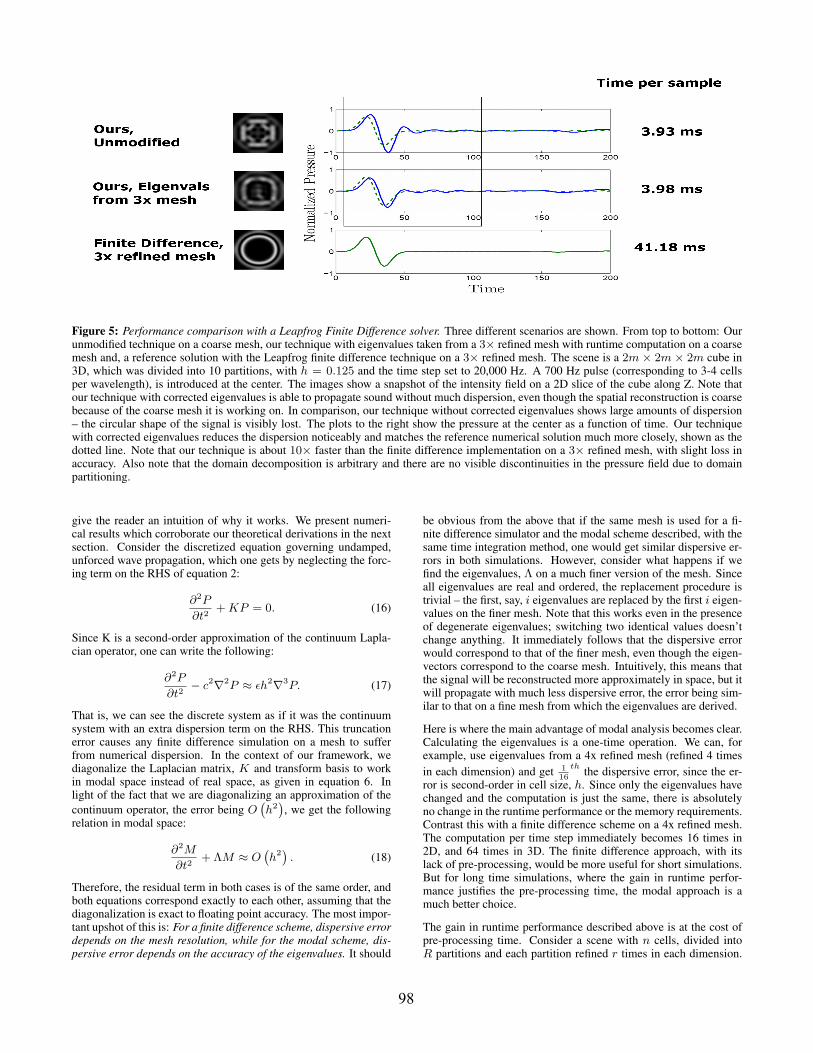
Figure 5: Performance comparison with a Leapfrog Finite Difference solver. Three different scenarios are shown. From top to bottom: Ourunmodified technique on a coarse mesh, our technique with eigenvalues taken from a 3× refined mesh with runtime computation on a coarsemesh and, a reference solution with the Leapfrog finite difference technique on a 3× refined mesh. The scene is a 2m × 2m × 2m cube in3D, which was divided into 10 partitions, with h = 0.125 and the time step set to 20,000 Hz. A 700 Hz pulse (corresponding to 3-4 cellsper wavelength), is introduced at the center. The images show a snapshot of the intensity field on a 2D slice of the cube along Z. Note thatour technique with corrected eigenvalues is able to propagate sound without much dispersion, even though the spatial reconstruction is coarsebecause of the coarse mesh it is working on. In comparison, our technique without corrected eigenvalues shows large amounts of dispersion– the circular shape of the signal is visibly lost. The plots to the right show the pressure at the center as a function of time. Our techniquewith corrected eigenvalues reduces the dispersion noticeably and matches the reference numerical solution much more closely, shown as thedotted line. Note that our technique is about 10× faster than the finite difference implementation on a 3× refined mesh, with slight loss inaccuracy. Also note that the domain decomposition is arbitrary and there are no visible discontinuities in the pressure field due to domainpartitioning.
give the reader an intuition of why it works. We present numeri-cal results which corroborate our theoretical derivations in the nextsection. Consider the discretized equation governing undamped,unforced wave propagation, which one gets by neglecting the forc-ing term on the RHS of equation 2:
∂2P
∂t2+ KP = 0. (16)
Since K is a second-order approximation of the continuum Lapla-cian operator, one can write the following:
∂2P
∂t2− c2∇2P ≈ εh2∇3P. (17)
That is, we can see the discrete system as if it was the continuumsystem with an extra dispersion term on the RHS. This truncationerror causes any finite difference simulation on a mesh to sufferfrom numerical dispersion. In the context of our framework, wediagonalize the Laplacian matrix, K and transform basis to workin modal space instead of real space, as given in equation 6. Inlight of the fact that we are diagonalizing an approximation of thecontinuum operator, the error being O
(h2)
, we get the followingrelation in modal space:
∂2M
∂t2+ ΛM ≈ O
(h2)
. (18)
Therefore, the residual term in both cases is of the same order, andboth equations correspond exactly to each other, assuming that thediagonalization is exact to floating point accuracy. The most impor-tant upshot of this is: For a finite difference scheme, dispersive errordepends on the mesh resolution, while for the modal scheme, dis-persive error depends on the accuracy of the eigenvalues. It should
be obvious from the above that if the same mesh is used for a fi-nite difference simulator and the modal scheme described, with thesame time integration method, one would get similar dispersive er-rors in both simulations. However, consider what happens if wefind the eigenvalues, Λ on a much finer version of the mesh. Sinceall eigenvalues are real and ordered, the replacement procedure istrivial – the first, say, i eigenvalues are replaced by the first i eigen-values on the finer mesh. Note that this works even in the presenceof degenerate eigenvalues; switching two identical values doesn’tchange anything. It immediately follows that the dispersive errorwould correspond to that of the finer mesh, even though the eigen-vectors correspond to the coarse mesh. Intuitively, this means thatthe signal will be reconstructed more approximately in space, but itwill propagate with much less dispersive error, the error being sim-ilar to that on a fine mesh from which the eigenvalues are derived.
Here is where the main advantage of modal analysis becomes clear.Calculating the eigenvalues is a one-time operation. We can, forexample, use eigenvalues from a 4x refined mesh (refined 4 timesin each dimension) and get 1
16
th the dispersive error, since the er-ror is second-order in cell size, h. Since only the eigenvalues havechanged and the computation is just the same, there is absolutelyno change in the runtime performance or the memory requirements.Contrast this with a finite difference scheme on a 4x refined mesh.The computation per time step immediately becomes 16 times in2D, and 64 times in 3D. The finite difference approach, with itslack of pre-processing, would be more useful for short simulations.But for long time simulations, where the gain in runtime perfor-mance justifies the pre-processing time, the modal approach is amuch better choice.
The gain in runtime performance described above is at the cost ofpre-processing time. Consider a scene with n cells, divided intoR partitions and each partition refined r times in each dimension.
98
Also note that we only need the first nR
eigenvalues of the refinedmesh for each partition. Thus the time taken for each partition is
proportional to nR
(nr3
R
)2
. Since this is repeated for R partitions,
the total time becomes n(
nr3
R
)2
. Observing that a full diagonal-
ization on the coarse mesh would take time proportional to n3, thenet gain in pre-processing performance becomes, Gain = R2/r6.Thus, given a particular scene, we select the value of R based on theone which yields the best runtime performance, based on the com-plexity analysis given in 4.3 and then select a value of r as high aspossible, to get the best accuracy while keeping the above relationin mind, so that the pre-processing requirements are tractable. Thisway, we are able to trade-off between runtime performance, accu-racy and pre-processing resources. As an implementation detail, inthis work, we have used the ARPACK [Lehoucq et al. 1997] eigen-value package for computing a selected initial part of the eigenvaluespectrum.
5 Results
In this section, we present the main results to demonstrate the ac-curacy and efficiency achievable with our approach. All the simu-lations were performed on an Intel Xeon Quad-Core 2.79GHz CPUwith 2GB RAM.
5.1 Accuracy: Interference and Diffraction
We evaluated the accuracy of our simulator on the basis of how wellit simulates the wave phenomena of reverberation, interference anddiffraction. As mentioned in the introduction, these phenomena arecritical for a physically correct simulation of sound in general envi-ronments. We first discuss our results for interference and diffrac-tion on a 2D double-slit experiment. The setup is shown in Figure 3.The image on the left shows the color-coded pressure amplitude inthe scene. A sound source is placed at the center-left of the domain(shown as a white circle), emitting a sine wave with fixed frequencyof 400 Hz. The domain boundary is fully reflective. The grid spac-ing for the spatial discretization of the domain is h = 1
8m, which
means we can handle up to ∼ 900 Hz with about k = 3 elementsper wavelength. An obstructing wall is placed in front of the soundsource at a distance of 4m. The wall has two symmetrically placedslits, each one cell wide ( 1
8m). A virtual screen is placed on the
opposite side of the wall, at a distance of 2.5m from the slits.
Sound waves traveling from the source first hit the wall and only asmall portion of it passes through the slits, which act as secondarypoint sources on the other side of the wall. This demonstrates thatdiffraction is properly captured by our technique. Next, sound fromthe two slits interferes throughout the domain, resulting in an in-terference pattern. The pressure field shows a near-uniform angu-lar distribution of maxima and minima, depending on where soundwaves interfere constructively and destructively, respectively. Thisresult clearly demonstrates that interference is also simulated cor-rectly with our technique. To quantify the accuracy of the resultingsound field, we compare the observed and theoretical sound inten-sity (square of the sound amplitude) along the length of the virtualscreen. The right side of Figure 3 shows the graphs for the soundintensity against the position on the virtual screen. Note the closeagreement between the positions of the expected minima and max-ima and the numerically computed values.
Figure 6: Visualization of reduced numerical dispersion. Compar-ison of numerical results from simulation on a coarse mesh withand without corrected eigenvalues from a 3× refined mesh on a 2Dscene. The images to the left show snapshots in time of the soundintensity in a square 2D domain with dimensions 6m × 6m andh=0.125m. The domain was divided into 10 partitions. A 500HzGaussian pulse is triggered at the center and spreads out, reflectsfrom the walls and interferes with itself at the center. Note that thecoarse simulation has a lot more “ringing,” as the signal shape isgradually lost over time, which corresponds to numerical disper-sion. This is more obvious in the last image. The plots to the rightshow the pressure at the center of the domain as a function of time.As shown in the insets, after the initial impulse is fed, the coarsesimulation has a high frequency tail, while for the simulation withcorrected eigenvalues, this is much less so. This shows that withcorrected eigenvalues, the dispersion is reduced.
5.2 Accuracy: Dispersion analysis and comparisonwith a finite difference solver
In order to clearly assess the benefit with our approach, it is im-portant to assess how it compares in terms of accuracy to a standardfinite difference implementation. In this section, we will briefly dis-cuss a second-order accurate in space and second-order accurate intime method for solving the wave equation numerically, and com-pare it against our method. This is done by performing a dispersionanalysis of both methods on a 2D square scene, for undamped, un-forced wave propagation. This scene has been chosen because it iseasier to perform dispersion analysis on rectangular domains.
We had theoretically motivated in Section 4.4 that the accuracyof our method with eigenvalues substituted from a refined meshshould be comparable to the accuracy of a finite difference methodon the refined mesh. The finite difference method we consider inthis work is the standard cell-centered second-order Leapfrog inte-grator. In particular, consider a square domain of size [0, 1]× [0, 1],discretized uniformly into N ×N cells. The cell size is thus givenby h = 1
N. Lets denote the pressure at the cell with coordinate
(ih, jh) at time step n by P ni,j . Then the finite difference integrator
is given by –
P n+1i,j = 2P n
i,j − P n−1i,j
+ c2∆t2
h2
(P n
i+1,j + P ni−1,j + P n
i,j−1 + P ni,j+1 − 4P n
i,j
)(19)
As a first step in the dispersion analysis, note that the wave equationcan be solved analytically for the square domain with Neumannboundary conditions. This is done by expressing the pressure in thedomain in the Cosine basis as –
99
P (x, y, t) =
N−1∑kx=0
N−1∑ky=0
m (kx, ky, t) cos (πkxx) cos (πkyy) ,
(20)where kx and ky are the wavenumbers (proportional to the in-verse of the wavelength) in the X and Y directions respectivelyand m (kx, ky, t) is the corresponding scaling coefficient. Plug-ging this into the wave equation (1) and assuming the forcing termon the RHS is absent, and solving w.r.t time, we get the importantrelation –
m (kx, ky, t) = Aeick(kx,ky)t + Be−ick(kx,ky)t,
k (kx, ky) = π√
k2x + k2
y.
(21)
The constants A and B depend on the initial conditions and are notrelevant here. The important quantity is k (kx, ky), which, gives theanalytically computed wavenumber, given the spatial wavenumbersin the X and Y direction. Carrying out a similar procedure withequation (19), by plugging in equation (20) and denoting all corre-sponding variables with a prime, we get –
Therefore, the numerical speed of propagation for differentwavenumbers is not the same as the analytical expression. Note thatfor every wavenumber (kx, ky), Limh→0k
′ = k, which is requiredfor consistency. The amount of numerical dispersion for a givenwavenumber, k =
√k2
x + k2y can be quantified by k′
k, called the
dispersion coefficient. Intuitively, the dispersion coefficient mea-sures how slow or fast a wave with a particular wavenumber wouldtravel on the mesh, compared to the speed of sound, c. Ideally, thedispersion coefficient should be 1 for all wavenumbers. Figure 4shows the dispersion coefficient of the finite difference scheme de-scribed above for increasing wavenumbers, k. Note that when thecell size, h is large, as on the coarse mesh, the dispersion is reallylarge for higher wavenumbers. This improves considerably on amesh which has been refined 4 times in both dimensions.
Till now we have discussed the Finite Difference technique wecompare against and its dispersion analysis. The dispersion anal-ysis of our method closely parallels the above discussion. ConsiderEquation (7) and assume the forcing term is 0. It is easy to see that
one gets a solution very similar as (21), with k′′i =
√Λi
c. Again,
one can obtain the dispersion coefficient by dividing by the analyt-ical expression for k given by (21). Figure 4 shows a comparisonof the dispersion coefficients obtained for our method and the fi-nite difference method for different cases. Firstly, note that as wastheoretically discussed in Section 4.4, the dispersion coefficientson a coarse mesh for our technique and the finite difference tech-nique follow the same trend, exhibit large amounts of dispersion forhigher wavenumbers. The most important fact to note, however, isthat the dispersion coefficients for the finite difference method on a4x refined mesh are very similar to that of our technique on a coarsemesh with eigenvalues derived from a 4x refined mesh. This cor-roborates the theoretical claims made in Section 4.4 that the accu-racy of the eigenvalues determines the dispersion of our techniqueand demonstrates that substituting eigenvalues from a refined meshdoes reduce the dispersion error with our technique without incur-ring extra runtime cost. At this point we emphasize again that this is
the chief advantage and main motivation for working in the modalbasis instead of real space.
5.3 Efficiency
To compare the performance and accuracy of our approach withthe finite difference scheme described above, we implemented bothin a common code-base. For the test scene, we considered a2m× 2m× 2m cube in 3D, with h = 0.125m and divided the do-main into 10 arbitrary partitions and initiated a 700 Hz pulse at thecenter. We would like to emphasize here that the partitioning neednot have any specific structure. Figure (5) illustrates the results weobtained. There are three cases we have considered: the bottomrow shows the results obtained with the finite difference scheme ona 3x refined mesh, and can be treated as a reference solution, thetop row shows our technique on a coarse mesh without using cor-rected eigenvalues, which can be considered a basic implementationand the middle row shows our technique with corrected eigenvaluesfrom a 3x refined mesh. Note that the accuracy of our technique isintermediate between the two. Although dispersion is still present,visible as the wavy tail after the initial signal, it is much smallercompared to the basic approach. The important thing to note is thatthis gain in accuracy comes at almost no reduction in performance.The timings on the right side of the figure show the time taken togenerate 1 sample of audio with the different techniques. It is clearthat our technique is about 10x faster for this scene. Also, note thatthere are no visible discontinuities in the field at the partition in-terfaces, which shows that partitioning is being handled accurately.Another demonstration of reduced dispersion with our techniquewith corrected eigenvalues on a 2D scene is shown in Figure 6.
5.4 3D Environment
To demonstrate the efficiency and robustness of our approach, wehave implemented our algorithm and tested it on a moderately com-plex architectural model. Figure 7 shows the results for a soundsimulation on the building. The user may move freely through themodel and all the sounds in the scene are passed in to a sound sim-ulator which implements all the techniques described in this paper.The physical dimensions of the building are 12m × 13m × 7m,which is about the size of a large hall. The grid spacing for spatialdiscretization on the coarse mesh is h = 1
8m. The total air volume
of the scene is approximately 600m3, which corresponds to about300,000 cells. The map was first partitioned into 300 partitions,each having about 1000 cells. For each partition, the eigenvalueswere corrected by using the eigenvalues from a 3x refined mesh,each with about 27,000 cells. The refinement factor was fixed sothat the matrix diagonalization did not take more than 2GB of mem-ory. The pre-processing was performed on a cluster, with each par-tition being processed on a separate node, in parallel. Each nodehas a 2.3GHz Intel EM64T processor with 4M L2 cache. The totaltime for pre-processing this scene was about 50 minutes.
Even though the pre-processing is expensive, it is still tractable.Following the analysis in Section 4.4, observe that dividing thescene into 300 partitions and then taking eigenvalues from a 3x re-fined mesh reduces the pre-processing time by 3002
36 ≈ 100 times.Therefore, the pre-processing requirements are reduced consider-ably, even though we are sacrificing some pre-processing efficiencyfor improved accuracy at runtime. The simulator takes about 300ms per sample of audio, at an audio update rate of 5000 Hz, whileconsuming about 1GB of memory. Note that the compute require-ments are high even when we are using a coarse mesh which isclose to the Nyquist threshold. In comparison, a finite differenceimplementation would require a 3x refined mesh, which would have27× 300, 000 = 8.1M cells.
100
Sound Signal Frequency Spectrum
!!"#
!
!"#
!!"#
!
!"#
!!"#
!
!"#
!
"#
"!
$%"#!&
'
(
)
$%"#!&
'
(
)
*
"#
"'
"(
$%"#!&
Small Scene:
Large Scene:
Source Signal:
Figure 7: Results for sound simulation on a complex architectural scene in 3D. The physical dimensions of the map are 12m× 13m× 7mand it has an air volume of 300,000 cells, which we partition into 300 partitions. We are able to perform simulations for frequencies up to1kHz on this map. The listener is at the player’s location. Note that the input sound is modified considerably by the environment dependingthe size of the space (small or large). Also note that the frequency content of the input signal is effectively filtered depending on the resonantproperties of the area of the map where the listener is located. Note the “reverberant tail” in both the simulated sounds.
The input signal was band-passed below 1kHz, since that is themaximum simulated frequency. Note the marked difference be-tween the input sound and the signal received by the listener. Thisshows that the input sound is modified considerably by the environ-ment depending the size of the space (small or large). The “tail” ofthe response shows that late reverberations (corresponding to hun-dreds of reflections) are being captured by the simulator. Also notethat the frequency content of the input signal is markedly differentdepending on how it interferes with itself after multiple reflections,which is crucially influenced by the area of the map where the lis-tener is located. To show the generality of our approach, we havealso performed the simulations on a different environment, shownin Figure 1. This map has about 290,000 elements and was parti-tioned into 290 partitions. The pre-processing for this scene tookabout 65 minutes. The sound simulation was carried out at an up-date rate of 5000 Hz. The time taken to generate one sample ofaudio at runtime was about 250 ms.
6 Conclusion
We have proposed an efficient and accurate technique for modelingsound propagation in an arbitrary 3D environment by directly inte-grating the wave equation. Our results show that important acousticeffects like interference, diffraction and reverberation are accuratelycaptured by our technique. Moreover, due to the combination of asimple and stable domain decomposition technique and a techniqueto reduce the dispersion on a coarse mesh by utilizing the eigenval-ues from a refined mesh, we are able to handle complex 3D sceneswith∼ 300, 000 elements and frequencies up to 1 kHz, while manyprevious numerical techniques have been demonstrated simulatingfrequencies only up to a few hundred Hz. We believe that furtheroptimization combined with the increased computing power of theupcoming many-core processors will enable our technique to per-form interactive simulation on 3D scenes with millions of elementsin the foreseeable future, enabling rapid design and simulation ofbuilding acoustics and offering a much more immersive auditoryexperience for virtual environments.
7 Acknowledgements
This work was supported by the Army Research Office, DefenseAdvanced Research Project Agency, National Science Foundation,RDECOM and Intel Corporation.
References
ALFORD, R. M., KELLY, K. R., AND BOORE, D. M. 1974. Accu-racy of finite-difference modeling of the acoustic wave equation.Geophysics 39, 6, 834–842.
ALLEN, J. B., AND BERKLEY, D. A. 1979. Image method forefficiently simulating small-room acoustics. J. Acoust. Soc. Am65, 4, 943–950.
ANTONACCI, F., FOCO, M., SARTI, A., AND TUBARO, S. 2004.Real time modeling of acoustic propagation in complex environ-ments. Proceedings of 7th International Conference on DigitalAudio Effects, 274–279.
BERTRAM, M., DEINES, E., MOHRING, J., JEGOROVS, J., ANDHAGEN, H. 2005. Phonon tracing for auralization and visual-ization of sound. In IEEE Visualization 2005.
BOTTELDOOREN, D. 1994. Acoustical finite-difference time-domain simulation in a quasi-cartesian grid. The Journal of theAcoustical Society of America 95, 5, 2313–2319.
BOTTELDOOREN, D. 1995. Finite-difference time-domain sim-ulation of low-frequency room acoustic problems. AcousticalSociety of America Journal 98 (December), 3302–3308.
DDM. http://www.ddm.org.
DEINES, E., MICHEL, F., BERTRAM, M., HAGEN, H., ANDNIELSON, G. 2006. Visualizing the phonon map. In Eurovis.
FUNKHOUSER, T., TSINGOS, N., AND JOT, J.-M. 2003. Surveyof methods for modeling sound propagation in interactive virtualenvironment systems. Presence and Teleoperation.
FUNKHOUSER, T., TSINGOS, N., CARLBOM, I., ELKO, G.,SONDHI, M., WEST, J. E., PINGALI, G., MIN, P., AND NGAN,A. 2004. A beam tracing method for interactive architecturalacoustics. The Journal of the Acoustical Society of America 115,2, 739–756.
KARJALAINEN, M., AND ERKUT, C. 2004. Digital waveguidesversus finite difference structures: equivalence and mixed mod-eling. EURASIP J. Appl. Signal Process. 2004, 1 (January), 978–989.
KARYPIS, G., AND KUMAR, V. 1999. A fast and high quality mul-tilevel scheme for partitioning irregular graphs. SIAM Journal onScientific Computing 20, 1, 359–392.
101
KINSLER, L. E., FREY, A. R., COPPENS, A. B., AND SANDERS,J. V. 1999. Fundamentals of Acoustics. Wiley, December.
KLEINER, M., DALENBCK, B.-I., AND SVENSSON, P. 1993. Au-ralization - an overview. JAES 41, 861–875.
KROCKSTADT, U. 1968. Calculating the acoustical room responseby the use of a ray tracing technique. Journal of Sound Vibration.
KUTTRUFF, H. 2000. Room Acoustics. Taylor & Francis, October.
LEHOUCQ, R., SORENSEN, D., AND YANG, C. 1997. Arpackusers’ guide: Solution of large scale eigenvalue problems withimplicitly restarted arnoldi methods. Tech. rep.
LOKKI, T. 2002. Physically-based Auralization. PhD thesis,Helsinki University of Technology.
MIN, P., AND FUNKHOUSER, T. 2000. Priority-driven acousticmodeling for virtual environments. In EUROGRAPHICS 2000.
MURPHY, D., KELLONIEMI, A., MULLEN, J., AND SHELLEY,S. 2007. Acoustic modeling using the digital waveguide mesh.Signal Processing Magazine, IEEE 24, 2, 55–66.
O’BRIEN, J. F., SHEN, C., AND GATCHALIAN, C. M. 2002. Syn-thesizing sounds from rigid-body simulations. In The ACM SIG-GRAPH 2002 Symposium on Computer Animation, ACM Press,175–181.
RAGHUVANSHI, N., AND LIN, M. C. 2006. Interactive soundsynthesis for large scale environments. In SI3D ’06: Proceedingsof the 2006 symposium on Interactive 3D graphics and games,ACM Press, New York, NY, USA, 101–108.
RINDEL, J. H. The use of computer modeling in room acoustics.
SABINE, H. 1953. Room acoustics. Audio, Transactions of the IREProfessional Group on 1, 4, 4–12.
SAKAMOTO, S., YOKOTA, T., AND TACHIBANA, H. 2004. Nu-merical sound field analysis in halls using the finite differencetime domain method. In RADS 2004.
SAKAMOTO, S., USHIYAMA, A., AND NAGATOMO, H. 2006. Nu-merical analysis of sound propagation in rooms using the finitedifference time domain method. The Journal of the AcousticalSociety of America 120, 5, 3008–3008.
SAVIOJA, L., RINNE, T., AND TAKALA, T. 1994. Simulationof room acoustics with a 3-d finite difference mesh. Proc. Int.Computer Music Conf , 463–466.
SAVIOJA, L., BACKMAN, J., JRVINEN, A., AND TAKALA, T.1995. Waveguide mesh method for low-frequency simulationof room acoustics. In 15th International Congress on Acoustics(ICA’95), vol. 2, 637–640.
SAVIOJA, L. 1999. Modeling Techniques for Virtual Acoustics.Doctoral thesis, Helsinki University of Technology, Telecom-munications Software and Multimedia Laboratory, Report TML-A3.
TSINGOS, N., FUNKHOUSER, T., NGAN, A., , AND CARLBOM, I.2001. Modeling acoustics in virtual environments using the uni-form theory of diffraction. In Computer Graphics (SIGGRAPH2001).
TSINGOS, N., DACHSBACHER, C., LEFEBVRE, S., ANDDELLEPIANE, M. 2007. Instant sound scattering. In Render-ing Techniques (Proceedings of the Eurographics Symposium onRendering).
VAN DEN DOEL, K., KRY, P. G., AND PAI, D. K. 2001. Foleyau-tomatic: physically-based sound effects for interactive simula-tion and animation. In SIGGRAPH ’01: Proceedings of the 28thannual conference on Computer graphics and interactive tech-niques, ACM Press, New York, NY, USA, 537–544.
VAN DUYNE, S., AND SMITH, J. O. 1993. The 2-d digital waveg-uide mesh. In Applications of Signal Processing to Audio andAcoustics, 1993. Final Program and Paper Summaries., 1993IEEE Workshop on, 177–180.