1

Master’s Degree Thesis

Accelerating Transformer Deep Learning Models on FPGAs using High-Level Synthesis

Supervisor : Prof. Luciano Lavagno Candidate : Mahmoud Bahmnai

Politecnico di Torino

April 2021

2

Astract

In the current electronic industry, logic synthesis that starts from RTL description has been the superior method to implement digital systems on both FPGAs and application-specific chips. But recently, High-Level Synthesis (HLS) has grown and now is the choice of hardware engineers and designers for the implementation of complex digital systems.

High-Level Synthesis or HLS is an automatic process that accepts synthesizable code written using high-level languages such as C, SystemC, OpenCL (Open Computing Language), and C++ and then transforming them into an RTL design. Finally, This design is then implemented on hardware devices such as FPGAs. FPGA has limited resources of hardware in terms of the logic cell, interconnection which contains wires that are routed to the power supply, clock, and signal nets.

In terms of language translation (Italian to English or vice versa) natural language processing, RNN (Recurrent Neural Networks) can be used but this method severely suffers from two issues: incapable of capturing very long term dependencies and also unable in order to parallelizing sequential computation flow. Consider that, models with multi-head attention such as Transformer have extreme effectiveness in order to capture the long-term dependencies in a variety of sequence modeling tasks.

Here in this project Transformers applied on FPGA in terms of performing and analyzing time, area, and power. The network designed with C++ and applied through the Vivado HLS tools on the FPGA board. this work has been depicted by designing a customized hardware accelerator for the Transformer by using a High-Level Synthesis. The tool is provided by Xilinx which is called Vivado HLS. This accelerator needs to be implemented on the board. For this, the PYNQ board has been chosen. It has a dual-core Cortex A9 processor.

3

List of Acronyms CPU

Central Processing Unit FPGA

Field Programmable Gate Array GPU

Graphical Processing Unit HDL

Hardware Description Language HLS High Level Synthesis IP

Intellectual Property LSTM

Long Short Term Memory PL

Programmable Logic PLAN Piece wise Linear Approximation PNYQ Python Productivity for ZYNQ RNN Recurrent Neural Network RTL Register Transfer Level VHDL VHSIC Hardware Description Language Vivado HLS Vivado High Level Synthesis

4

Aknowledgements

I am grateful for the cooperation and support from the professors and students of our research group, specially head of research group and my thesis supervisor Prof. Luciano Lavagno which with his patient and guidance made this work feasible.

I dedicate this work which is the outcome of months of research to my parent and all professors from all years of my academic career; Ihavetosay“thankyou”tothemfortheirloveandsupportthroughoutmylife.Icannotlistallthenameshere,butyouarealwaysonmymind.

Turin,April7th,2021

5

Contents

1.INTRODUCTION .............................................................................................................................. 8

1.1.HIGH-LEVEL SYNTHESIS, VIVADO HLS ................................................................................. 8

1.2.DESIGN FLOW ............................................................................................................................... 9

1.3.CONSTRAINTS IN HLS ................................................................................................................. 9

1.4.RTL VALIDATION AND EXPORT ............................................................................................ 11

2.1.LOOP UNROLLING ..................................................................................................................... 12

2.2.INTERFACES ............................................................................................................................... 14

2.3..PIPELINING ................................................................................................................................ 17

2.4.ARRAY PARTITIONING ............................................................................................................ 18

3.1. RNN ............................................................................................................................................... 21

3.2.BERT .............................................................................................................................................. 21

3.3.ROBERTA ..................................................................................................................................... 22

3.4..DISTILBERT ................................................................................................................................ 22

3.5.XLNET ........................................................................................................................................... 22

4.TRANSFORMERS:.......................................................................................................................... 23

4.2. SOFTMAX .................................................................................................................................... 25

4.3.WORD2VEC .................................................................................................................................. 25

4.4.SELF ATTENTION: ..................................................................................................................... 26

6

4.4.1.ATTENTION CALCULATION: ............................................................................................... 26

4.6.FEED FORWARD: ....................................................................................................................... 26

4.7.ADD AND NORMALIZATION.................................................................................................... 27

5.QUANTIZATION: ........................................................................................................................... 28

5.2.FP32 VS. INTEGER ...................................................................................................................... 28

5.3.IP BLOCK GENERATION .......................................................................................................... 31

6.CONCLUSIONS ............................................................................................................................... 32

6.1.SUMMARY .................................................................................................................................... 32

6.2.RESULTS....................................................................................................................................... 32

7.1APPENDIX C ATTENTION LAYER…………………...…..……………………………………..34 UTILIZATION DESIGN INFORMATION……………...………………………………………40 BIBLIOGRAPHY…………………………………………..……………………………………46

7

List of figure Figure1:streaming mechanism Figure2:Interface Figure3:Interface with different bank Figure4:Interface with different bank Figure5:Pipeline cycles Figure6:Array partitioning instruction Figure7:RNN procedure Figure8:Comparison of transformer models Figure9:Transformer architecture Figure10:Decoder and Encoder Figure11:Word2Vec concept Figure12:Utilization before quantization Figure13:Utilization after quantization Figure14:Resource usage before quantization Figure15: Resource usage after quantization Figure16: Quantization architecture Figure17: Quantization methodology Figure18: IP export report

8

1.Introduction

Right now there are over 6000 languages which are spoken in the world. A key parameter that humans can communicate to each other or do business or travel is translation. a simple idea about translation is translating sentences from for example Italian to english word by word till the last word. If this method applied as translation technique it has a really low precision and even in some case can changes the meaning of the sentence. To solve this issue RNN has been introduced as a model for NLP (natural language processing) usages. By relying on RNN applications such as next-sentence prediction, question answering, reading comprehension, sentiment analysis, paraphrasing, machine translation, document summarization, document generation, named entity recognition, speech recognition and biological sequence analysis could be process.

In this thesis, this work has been depicted by designing a customized hardware accelerator for the Transformer by using a High-Level Synthesis. The tool is provided by Xilinx which is called Vivado HLS. This accelerator needs to be implemented on a board. For this, PYNQ board has been chosen. It has a dual-core Cortex A9 processor.

High-Level Synthesis transform a high-level language (C, C++ or SystemC) design specifications into an RTL implementation that can be further synthesized for hardware construction on ASIC or FPGA device. High-Level Synthesis is an automated design process, to better understand this process.

1.1.High-Level Synthesis, Vivado HLS

High-Level Synthesis is an automated design procedure that converts a high-level design, mainly in C/C++ or SystemC, to optimized RTL for hardware implementation. Here in this project, the Vivado HLS tool is used that is provided by Xilinx. Xilinx High-Level Synthesis is a tool that Vivado HLS converts a C model into a Register Transfer Level (RTL) implementations which synthesizes into a Field Programmable Gate Array (FPGA) under Xilinx standards. Users can write C requirements in C++, SystemC or an OpenCL API kernel. This FPGA performs a desirable parallel architecture with advantages in order of cost, performance and power consumption compare to the traditional processors.

In fact, HLS offers a method that hardware and software providing the following benefits:

9

enhance productivity for hardware designers. Hardware designers are more open hand in order to design complex architectures. It is also capable of the developer to develop different multi-architectural designs without changing the C modules. This enables design space exploration and provides needs in finding the optimal implementation.

On other hand improved system performance for software designers. They have the capability to accelerate the intensive parts of their algorithms, which basically take a lot of calculation on a goal which here is focusing on FPGA.

1.2.Design Flow

With the Xilinx Vivado HLS tool first, you can create your design and optimize it and then generating an IP block that can be integrated into a hardware system. This IP block could be defined as a hardware accelerator which has been done in here this thesis. All parts of the design have been performed by C language, but in the case of using Vitis (which has all features of Vivado plus some new features) there would be a possibility to add modules in python language.

Vivado HLS design flow can be expressed:

In High-Level Synthesis executing C algorithm simulates the function to verify its working correctly in terms of functionally and then Synthesize the C algorithm into an RTL implementation. Optimization by use of directives and constraints can be added up to direct the synthesis process to implement a special optimization. It also generates reports in order hardware resource utilization, timing, and analyze the design in all aspects. Vivado HLS uses the C test bench to simulate the C functionality to synthesize and to validate the RTL output by use of C/RTL Co-simulation and Packaging the RTL implementation in a selection of IP packages.

1.3.Constraints in HLS

Vivado HLS is able to support the most kind of the C language but there are still some constraints that are not accepted. so these constraints could not be synthesized and can be finalized with an error during the design flow. For the design that would be synthesizable, the following modifications should be done in the code.

First of all, the function inside the C code should contain the whole functionality of the design. All the function call should be provided with respect to the Vivado rolls, not the operating system. One another thing that should be considered is to modify C constructs in terms of being

10

fixed size. Implementations of those constructs have to be unequivocal. Let's take a look at some constructs which can’t be synthesized in Vivado HLS.

• Standard Libraries: Many of the C++ standard libraries use dynamic memory allocation (Malloc) and recursive function. Accordingly, it could not be synthesizable as well. Memory allocation system calls as mentioned above are not supported and should be removed from the design code before synthesis. All type of system calls which manage memory allocation within the system, such as, free() and malloc() are using resources which exist inside the memory of the operating system and they are generated and released during the run time of the operating system that does not support by Vivado.

• System Calls: There are some function calls that are related to the operating system and they are not synthesizable because this kind of function has no impact directly on the final design. therefore Vivado HLS ignore them. some of these functions are as follow: time(),getc(),sleep(),printf().

• Pointer constraints: Vivado High-Level Synthesis does not support pointer casting, except if it would be between native C types. the pointers defined by the function are also not supported. But in order to synthesize, pointer arrays are supported.

11

1.4.RTL Validation and Export

In order to simulate the design, Vivado HLS uses the C test bench to verify the functionality of the top-level function. then, it automatically again uses the C test bench to validate the RTL output using co-simulation. Vivado HLS creates the files required to use the C testbench during the co-simulation. When validation has been complete, the console displays a special message to confirm the validation finished successfully. the testbench forces the design and if it returns a nonzero value, Vivado HLS reports that the simulation has been failed. Vivado creates the basic foundation to provide the C/RTL co-simulation and then executes the simulation by use of one of the supported RTL simulators.

After all synthesizing and simulation has been done correctly, the last step here in the Vivado HLS design flow is to make the package as a RTL output as an IP. Here are some options to export the final RTL output files as IP in any of the following Xilinx formats. Vivado is able to export the RTL as an IP with formats such as Vivado IP Catalog, System Generator for DSP, and Synthesized Checkpoint. the final output file format would be .Xo .

There is a possibility to execute logic synthesis from inside the Vivado HLS to evaluate the final design of RTL and its implementation. This confirms that the design can provide our requirements or not before the final export for hardware in order to utilizations and timing.

this project composed of 4 different modules and one Top module to connect all the other modules. all modules have their own testbench and they have been simulated and synthesized separately to confirm that they are working as well as expected.

another approach for our design to decreasing the latency is using streaming data interface. Without this interface when the design wants to read a data from DDR memory, it produces a long latency and when the number of requested data being high then the total delay will increase dramatically. The principal operation of this core allows the write or read of data packets to or from a device without any concern over the AXI4-Stream interface signaling. You can easily manage the AXI4-Stream interfaces as they are transparent.it is configurable at most 512-bit that the FIFO width could be 32 bits. This core has been designed to develop memory-access to an AXI4-straem interface which is connected to other IP.

12

Figure1:streamingmechanism

Streaming interface directly controlled with DMA (direct memory access) it means DMA streams the data from the DDR memory at each clock cycle you can access to the required data. One of the problems that I faced during streaming was ERROR: [SYNCHK 200-92], this error means axi streams are uni-directional and write-only and there is not possibility to doing read/write on the same stream which by considering this point the problem has been solved.

2.1.Loop unrolling Instead of using single collection of operations, by unroll loops there is ability to create multiple independent operations. This pragma by creating multiples copies body of the loop transforms loops in the RTL that allows some of the loop or all loops occur in parallel. in the C/C++ functions by default Loops are kept rolled. Whenever loops are rolled, then by synthesizing it will create logic for one iteration of the loop, and then RTL will execute the logic for all iteration of the loop respectively. A loop is executed for all number of iterations determined by the loop variable. The number of iterations has also to be impacted by logic inside the body of the loop ,for instance break conditions or modifications to a loop exit variable. To increase data access and throughput by using the UNROLL pragma you can unroll loops. The UNROLL pragma lets the loop to be completely or partially unrolled. completely unrolling the loop creates a copy of the loop in the RTL design for all loop iterations, consequently, the entire loop can be run simultaneously. Partially unrolling a loop allows you to determine a factor N, to

13

create N copies of the loop, and therefore decrease the loop iterations. In term of unrolling a loop completely, the loop bounds should be known at compile-time and it is not required for partial unrolling. Partial loop unrolling does not need N to be a factor of the maximum loop iteration count. Vivado HLS automatically adds an exit to ensure that partially unrolled loops are functionally similar to the original loop. To getting know more about this pragma let take a look at some code: For (int i=0; i < y; i++){

pragma HLS unroll factor=2 Z [i] = a[i] + b [i]; } At the mentioned code above, by applying pragma HLS unroll factor 3, at each iteration it will run simultaneously 2 loop. Lets take look how the above code work in term of functionality: For(int i=0; i<y: i++){ Z[i]=a[i] + b[i]; If (i+1 >= y) break; Z[i+1]=a[i+1] + b[i+1] } If take a closer look at the code, we can clearly observe that all the iterations of the loop are independent of each other. In fact, each addition is done on different elements of the input arrays and it is stored on different elements of the output array. therefore, is it possible to perform multiple additions in parallel on different elements? yes, and the answer to it, is by unrolling the loop. Loop unrolling in practical means unrolling the loop iterations so that, the number of iterations of the loop decreases, and the loop body performs extra computation. This technique let the design to expose extra instruction-level parallelism which Vivado HLS can exploit in order to hardware implementation. The pragma should be placed directly within the loop that we wish to unroll. The pragma also allows determining the unrolling factor by which we want to unroll the loop. consider that the unrolling factor can be any number from 2 up to the number of iterations of the loop. If the factor parameter is not defined, Vivado HLS tries to completely unroll the entire loop. However, this could be achieved only if the number of iterations is constant and not dependent on dynamic values within the function. To realize how Vivado HLS achieves this, we can look at the analysis report. Here we can clearly observe the Vivado HLS was able to schedule the execution of the two floating-point additions as like as the load and store operations completely in parallel! therefore this optimization comes at a cost. In term of performing the two floating-point additions fully in

14

parallel, it requires two floating-point adders in the hardware design which increase the overall resource consumption of the kernel. Indeed, if taking a look at the resource estimation report we can clearly observe the two floating-point adder instances and their corresponding resource consumption. In more complex designs it is very significant to consider the impact on resource consumptions when applying optimizations to the kernel. for instance, unrolling by a factor of 2 creates a straight 2x reduction in the latency of the loop at the cost of 2x more resources for its implementation. consequently, in some cases, it could not be possible to achieve this ideal in terms of latency improvement. When performing loop optimizations, there are two potential problems that require to be considered: The first one, constraints on the number of available memory ports and hardware resources, the second one is available loop-carried dependencies. Disadvantage of unrolling and how to face with it: At the first glance at unrolling method the basic idea comes in mind that why we do not unrolling all the loops by the maximum value of factor (number of loop iteration). the point is when a loop unrolled by at least factor 2, the required hardware doubled and consequently power consumption increase. So in term of unrolling the main point which should be considered is hardware limitation. The best idea to using this pragma is first start to find out the most important loop and then applying the unrolling just in most inner loop and then controlling the remained hardware and if there would be enough hardware apply it on other loop. 2.2.Interfaces once the suitable interfaces defined, SDAccel automatically generates FPGA design then connects the kernel module to the AXI interconnects of the shell. The kernel interfaces could be defined for special reasons. In general, for each argument, for example, a, b and res, it defines a couple of Master AXI and AXI Lite interfaces. The AXI Lite interface usage is to determine the offset at which the data resides in the onboard DDR and it is configured during initialization. The AXI Master interface is the actual interface used by the kernel to deliver data to/from the DDR memory. consider that it is possible to specify interfaces for scalar arguments, like a simple integer argument. In this case, a single AXI Lite interface is enough, the value of the scalar would be set on kernel initialization before the execution of the kernel. In addition to the argument interfaces, it is also mandatory to specify an AXI lite interface associated with the return, that is needed in order to specify the suitable signals to control the status of the kernel. For each HLS interface pragma, it is possible to define a bundle name. All the interfaces associated with the same bundle have been grouped to the same AXI interface. consider that SDAccel requires a single AXI late interface port. meanwhile, all the AXI LITE pragma should refer to the same bundle that here I named “control”. On the other hand, it is possible to determine multiple AXI master interface ports.

15

An example about access to DDR and with AXI and read from it and write to it:

Figure2:Interface By doing different bundle each interface connects to the different memory bank, then the value “a” and value “b” read-write exactly at the same time in parallel:

Figure 3 : Interface with different bank

Figure 4 : Interface with different bank

16

In this figure gmem0 and gmem1 work in parallel in term of timing

When implementing the last design with SDAccel, the software automatically define the Master AXI port to one of the DDR banks. otherwise, depending on the target platform, multiple DDR memory banks could be available and SDAccel allows to bind different AXI master interfaces to different DDR. This effectively lets to make full usage of the available bandwidth to the DDR bank by reading and writing in parallel across multiple banks. In order to leverage multiple memory banks, at the first step, we need to define multiple AXI master ports. To do it, it can simply bundle the arguments using different bundle names. In this example, I am targetting an Alpha-Data which features two memory banks. Hence, it can optimize memory transfers by the use of two distinct interfaces for reading the values of the input a and b. Here, specified “gmem0” for argument “a” and “gmem1” for argument 1. Finally, argument res is still bound to “gmem0”. As mentioned previously, the “memcpy” calls effectively create loops that read all the data elements in a row. In terms of reading in parallel both arguments a and b, it can be instructing Vivado HLS to merge the loop that gets created by the use of two memcpy. This is done by encapsulating the two “memcpy” call within a simple block using churly brackets and using the pragma HLS LOOP MERGE. this pragma tries to merge all the top-level loops encountered within the basic block in case that the pragma is placed. By observing the performance report from Vivado HLS, it can be now noticed that the two “memcpy” loops were collapsed into a single loop taking the same amount of iterations. If we look at the schedule, we can realize that the read operations on “gmem0” and “gmem1” are actually performed in parallel. At this point we have created a kernel with a couple of AXI master interfaces, but, in terms of full design implementation, we still need to tell SDAccel how to connect the interfaces with other memory banks available on the platform. In order to do it, we can set the «sp» argument when running the link phase with the xocc Xilinx compiler. This concludes that on interface optimizations. We first described the types of architecture targeted with the SDAccel and focused on the memory transfer operations included in the workflow of an SDAccel application. Then, it presented 3 type of optimizations for the communication between the kernel and the on-board DDR memory which are: memory bursts, maximization of AXI interface data width and the usage of multiple memory banks.

17

2.3.Pipelining Pipelining lets operations happening at the same time.in this method each execution step does not need to complete all operations before it starts next operation. To pipelining Functions or loops are pipelined PIPELINE directive should be used. The directive is defined in the place that constitutes the function or the loop. The start points of interval defaults to 1 if not declared but may be clearly specified. Pipelining is applied just to the specified area and not to the hierarchy. However, all loops which are in the hierarchy are automatically unrolled. Any sub-functions which is in the hierarchy, the specified function should be pipelined individually. In case that the sub-functions are pipelined, the pipelined functions can take benefit of the pipeline performance. subsequently, any sub-function under the pipelined top function which is not pipelined, could be the limiting factor in term of pipeline performance. There is a difference between pipelined functions and loops behavior. • pipelined functions: the pipeline runs all the time and never ends. • pipelined loops: pipeline executes till all iterations of the loop are completed.

Figure 5 : Pipeline cycles

Every stage computes a partial result of the operation and sends its data to the next level. Hence, if think about how this loop is executed in hardware, we can clearly observe that we are under-utilizing our resources. In fact, a given stage of the floating-point adder is executed once every 10 cycles, which means that it is used only 10% of the time! In order to enhance performance

18

as well as resource utilization, we can pipeline the loops, then each loop iteration starts as soon as possible instead of waiting for 10 cycles. By use of loop pipelining, we switch from a sequential execution of loop iterations to a pipelined execution that the loop iterations are overlapped in time. The number of clock cycles between two consequent iterations of a pipelined loop is referred to as Initial Interval, or II. The minimum possible Initial Interval that can be achieved for a pipelined loop is 1. It means that each loop iteration can start at every cycle. therefore, depending on the loop being pipelined, it should not be possible to achieve the ideal Initial Interval of 1 cycle. When achieving an initial interval of 1, it means after the initial time needed to fill the pipeline, all the levels of the operators inside the loop are completely utilized at all clock cycles. First, when all the iterations are executed in sequence, the final latency of the loop could be calculated by product of the Iteration Latency, mentioned as IL, by the Number of iterations, or trip count, N of the loop. In other words, the latency of the pipelined loop can be derived as follow. We need Initiation Interval times N–1 cycles to start the first N–1 loop iterations, by adding the time needed to complete the last iteration that takes 10 cycles, that is the iteration latency of the loop. consider that, compared to unrolling, loop pipelining does not considerably increase the resource consumption of our design, in fact with pipelining we are making better use of under-utilized hardware resources. With Vivado HLS we can use the HLS PIPELINE pragma inside the loop which we want to pipeline. As we can observe from the latency report, The 1 cycle difference compared to the previous formula is due to the fact that Vivado HLS accounts for such cycle inside the function body instead of the loop itself. a function which is pipelined continuously read new input and write new output. In contrary, because first loop should finish all the operations inside the body loop before starting the next loop, a pipelined loop causes a bubble in data stream. For instance a point that no new input is read as the loop completes the execution of the final iterations, and a point which no new output is written as the loop starts new loop iterations. Pipelines continue to execute until data is available at the input and If there is not any data available to process, pipeline will stall. 2.4.Array partitioning: Arrays are defined as block RAM that only has at most two data ports. This can reduce the throughput of a write or read (or store/load) intensive algorithm. The bandwidth can be increase by splitting the array (one block RAM as a resource) into some smaller arrays (some block RAMs), consequently extending the number of ports. Arrays are partitioned by use of the ARRAY_PARTITION directive. Vivado_HLS prepares three kinds of array partitioning, as depicted in the following figure. The three styles of partitioning are: • block: The original array is split into same-sized blocks of elements of the original array. • cyclic: The original array is split into the equal size blocks elements of the original array. • fully partitioning: The default is to split the array into its exclusive elements. This relates to resolving a memory into registers.

19

we have already seen that within a rolling the factor of 2 we managed to reduce the loop latency by a factor of 2. compared to the implementation that only uses loop pipelining. In fact within a rolling factor of 2, the loop creates two computations in parallel at each iteration. In this kind of computation are also pipelines with an initiation interval of 1 clock cycle. But when it tried to boost performance more inside a rolling factor of N, we got almost the same performance. In fact, while there is the trip count, we also double the initial interval. In addition, even if it has a small impact, the iteration latency is also raised by one clock cycle. The problem comes from the number of memory ports available for reading/writing data into the local arrays. by default each local array gets mapped to local memory on the FPGA up to 2 memory ports for reading/writing operations. so how we can overcome these limitations? It has mentioned that each array gets mapped to its own local memory on the FPGA, So why do not using multiple arrays to increase the number of memory boards? First, in terms of better visualize the problem, it helps to manually unroll the loop instead of using the HLS unroll pragma. specially, we need to access the element at position i, i+1, i+2 till i+N. Since the local memories just accept two ports, it means that we can only access the elements at position i and i+1 in one clock cycle and access i+2 and i+3 in the next iteration. It is also considerable to note that the value of i increments with the step of last loop iteration value in every cycle. when the elements that need to access change from iteration to iteration. In terms of being able to achieve an initiation interval of one clock cycle, a way to access elements 1, 2, 3, and so on are needed in parallel, as well as elements 5, 6, and …, N in parallel and so on. To achieve this, it could possible by applying the array partitioning technique. The overall idea is to reorganize the data of the original array into 2 or even smaller arrays or better partitions so that all partitions are mapped to their own memory with these corresponding read/write ports. The key element here is to decide how to reorganize that data. the best idea is to perform cyclic partitioning. Especially, here performed cyclic partitioning, It means that by creating partitions from the original array. By using cyclic partitioning, the data from the original array is going out to the partitioning a cyclic style. The first element is mapped to the first partition. The second element is mapped to the second partition, then the cycle repeats. all the accesses to the original arrays at addresses I, substituted with accesses to the first partitions. And also the accesses to i+1, substituted by accesses to the second partition, and so on. consider also when accessing the elements inside the partitions, also needs to divide by N (example of a number of iteration) the value of variable i. Also, need to be sure that the data coming from the external DDR memory bank gets well stored in the way intended. similarly, we need to send the data toward the same order we had before partitioning. First, we perform all partitions, then we need to change the logic for reading the data from the DDR bank memory. Instead of using a simple mem copy, here by writing a pipeline loop that at all iterations reads one value from the external DDR and then stores it in the correct partition of the local array. In terms of understanding the correct partition to use for the element at the address i of the first original array.

20

Figure 6: Array partitioning instruction

In fact, when using cyclic partitioning with the factor F, the element at address i from the first original array will store partition number i modulo F at address i divided by N. consider that here means integer division. The final result of an integer division is the result of division without the fractional part. Once the data read, then we can now define the calculation using vector. At the end, also needs to send back the results. To do it, we need to collect the data from the partitions of local results and send them to the external memory bank DDR. The logic here is the same as the one used for reading the data from the memory DDR bank. by creating a pipeline loop and at all iterations we fetch the current value from one of the partitions. finally, we write the value to the external DDR. Again, by using the modulo and the integer division operations to retake the correct value from the partitions. Thanks to the partitioning method, every iteration of the loop access exactly 1 element from each partition, which has its own memory port. Finally, it can define all the read/write operations in parallel and make us able to achieve the ideal initial interval of one clock cycle, but is there a simple way to achieve the same result without the need to rewrite all this long logic in a coded manner? the answer is yes. the array partitioning pragma prepared for this purpose. For cyclic and block partitioning, factor option defines number of arrays which are created. In case of using factor of 2, the array has been divided into two smaller arrays. If the number of elements in the array is not an integer multiple of the factor, the final array has lower elements.

21

3.1. RNN It composed set of algorithms which behave as like as human brain and it designed in a way that can recognize patterns through labelling and clustering input data with machine perception. All the real data such as image, text, sound first should convert to the vectors and then it recognize them as a numerical pattern. Recurrent Neural Network is extension of feedforward NN which has its own internal memory. RNN perform same function to the all inputs but its output related to the previous computation and when the output has been generated then it will send it into the recurrent network and to make final decision it relies on actual input (current value) and the output which learned from past input.

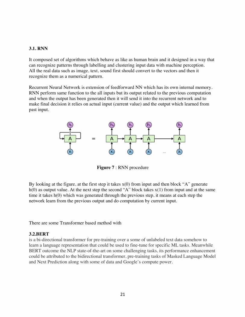
Figure 7 : RNN procedure

By looking at the figure, at the first step it takes x(0) from input and then block “A” generate h(0) as output value. At the next step the second “A” block takes x(1) from input and at the same time it takes h(0) which was generated through the previous step, it means at each step the network learn from the previous output and do computation by current input. There are some Transformer based method with 3.2.BERT is a bi-directional transformer for pre-training over a some of unlabeled text data somehow to learn a language representation that could be used to fine-tune for specific ML tasks. Meanwhile BERT outcome the NLP state-of-the-art on some challenging tasks, its performance enhancement could be attributed to the bidirectional transformer, pre-training tasks of Masked Language Model and Next Prediction along with some of data and Google’s compute power.

22

3.3.RoBERTa Introduced at Facebook, optimized BERT method RoBERTa, is a retrained version of the BERT with enhanced training methodology which is 1000% more data and compute power. To enhance the training procedure, RoBERTa method will removes the Next Sentence Prediction (NSP) task from BERT’s pre-training and introduced dynamic-masking so which the masked tokens modified during the training epoch. Big batch-training sizes are also found to be more advantageous in the training procedure. basically, RoBERTa uses over 160 GB of text for pre-training, including 16GB of Books and Wikipedia used in BERT. an additional data which included is CommonCrawl News dataset (around 63 million articles, 76 GB), Web text corpus (38 GB) and Stories from Common Crawl (31 GB). This connect with massive 1024 V100 Tesla GPU’s running for a day. 3.4.DistilBERT learns a distilled version of BERT, re-training 97% performance but using just half of parameter. explicitly, it does not has any token-type embedding, pooler and retains just half of the layers from Googles BERT. DistilBERT method uses a technique called distillation, that approximates the Google’s BERT, for instance the large neural network by a smaller one. The idea is once a large neural network has been trained, its output distributions could be approximated using a smaller network. This is similar to posterior approximation. One of the key optimization functions which used in Bayesian Statistics is Kulback Leiber divergence and has naturally been used here as well. 3.5.XLNet is a large bi-directional transformer which uses improved training method, more data and more computational power to achieve better result than BERT prediction on over 20 language tasks. To enhance the training, XLNet introduces permutation language model, where all the tokens have been predicted but in random order. This is in contrary to BERT’s masked language model which just the masked (around 15%) tokens are predicted. This is in contrast to the traditional language models, which all the tokens were predicted previously in sequential order instead of random one. This helps the model to learn bi-directional relationships, therefore better handles dependencies between words. In addition, Transformer XL used as the base architecture, which showed acceptable performance even in the absence of permutation based training. XLNet was trained with around 130 GB of textual data and 512 TPU chips running for 2.5 days.

23

Figure 8 : Comparison of transformer mode 4.Transformers: In term of neural machine translation a ubiquitous method to improve the performance is using attention concept. Transformer is a model that uses attention to boost up velocity by training the model. By comparing the models, transformer shows that has better performance in neural machine translation in some specific tasks. Most beneficial advantage of transformer is capability of parallelization. Google is a company which introduced this model and they used it in their cloud TPU as reference model. Let’s break the design and going more in detail to analysis the model.

24

Figure 9 : Transformer architecture

The first two main components are encoder and decoder which each one consists of stack of encoders and stack of decoder that the number layers in both decoder and encoder should be the same and identical in term of structure. By opening up encoder we can see it consists of two sublayers which named Feed Forward Neural Network and Self-Attention. With respect to the model hierarchy the input flow first to the Attention then its output fed the Feed Forward layer.

Figure 10 : Decoder and Encoder

25

Considering the application of this thesis which is NLP, first all the words in the input should turn into the vectors. This transformation is essential because most machines need all their input as vector instead of string that it can works properly. This technique called Embedding word to transform phrases from vocabulary to required vectors -this vectors are real numbers- aim to generate vectors with lower dimensional space. Word vector are used to taking what does the text means out from the entire text to make neural network able to understand it and it should be conscious about the similarity and the different between words in term of contextual meaning.

4.2. Softmax is a computational function which converts a vector of numbers into a vector of probabilities, in which the probabilities of each value are proportional to the related scale of each value in the vectors.

The most common use case of the softmax in applied ML is its use as an activation function in a neural network model. In fact, the network has been configured to output N values for each class in the classification task, and the softmax is used to normalizing the outputs and then converting them from weighted sum values into the probabilities which sum to one. Each value in the output of the softmax is interpreted as a probability of membership for each class

.4.3.Word2Vec

The input phrases are going through as one-hot encoded vectors. it goes into (hidden layer) of linear units, consequently go into the Softmax layer to make a prediction. The idea used is to first train the hidden layer weight to find effective representation for words. This matrix is often named embedding matrix, and can be queried as a look-up table.

One desirable feature of embeddings is because they’re represented as numbers of contextual similarities between words, by doing numerical operation between vectors we can reach to meaningful context. an example is subtracting the ‘notion’ of “King” from “Man” and adding the notion of “Woman”. The final answer depends on how the design trained before, but you’re eventually see one of the top results being the word “Queen”.

Figure 11 : Word2Vec concept

26

4.4.Self attention:

“The student didn’t go to Politecnico because it was closed”. In this sentence the “it” refers to the Politecnico. Understanding this kind of refers are simple for human but for machine is not simple as like as human. The duty of attention layer is processing “it” to associate it with Politecnico. In this case because the model processes all the input words, attention layer lets it to take a look better at the all words position and their sequence to do encoding words with more accuracy. 4.4.1.Attention calculation: At the first phase of calculation in attention layer, it creates three vectors for each input of the encoder -which are embedding of each word- that they called Key, Value and Query. All those three vectors calculated by multiplying matrices which trained before by embedding words output. Pay attention that those vectors smaller than embedding vector and mentioned matrices in term of dimension because the dimensionality of embedding word and encoder input vectors are 512 and by multiplying them, the size of Query, Key and Value reach to 64. What are the key, value and query? In term of self-attention calculation we need score of each word in sentence. This score will obtain by taking dot-product of query and value of a each word. For instance the word which placed at the first position of the sentence (position 1) its score calculated by dot-product of q1 and k1 and the second one would be dot-product of q1 and k2. At this phase score should divide by 8 (the square root of the key vectors which declared above 64). This provide more stable gradients, consequently send the result through a softmax operation. The duty of Softmax here is to normalizing the scores which means to be sure they’re all positive and add up to one. This Softmax score specify how much each word will be reliable at this position. In other word each word at this position has the most softmax score, but sometimes it’s better to consider another word that is relevant to the actual word. So now scores are ready and this is the time that softmax score should multiply by value vector and then by summing up weighted value producing output of self-attention for just first word. 4.6.Feed Forward: The feed-forward layer weights which are trained during training and the exact same matrix are applied to each respective token position. Since it is applied without communication with or inference by other tokens position it is an extremely parallelizable part of the model. The duty and purpose are to process the output from one attention layer in such a way to better fit the input for the next attention layer.

27

4.7.Add and Normalization State of the art deep neural networks generally requires many days of training. It is possible to speed up the learning by computing gradients in different subsets of the training cases on different machines or by splitting the neural network itself over, many machines, but this can require complex software. It also tends to lead to rapidly diminishing returns as the degree of parallelization increases. An orthogonal approach is to change the computations performed in the forward pass of the neural network to make learning easier. currently, batch normalization has been proposed to reduce training time by adding extra normalization stages in deep neural networks. The normalization standardizes all summed input using its mean and its standard deviation across the training data. Feedforward neural networks trained by using batch normalization converge even faster with simple SGD. In addition to training time improvement, the stochasticity from the batch statistics serves as a regulariser during the training step. Despite, batch normalization requires running averages of the summed input statistics. In feed-forward networks with fixed depth, it is straightforward to store the statistics independently for each hidden layer. However, the summed inputs to the recurrent neurons in an RNN often vary with the length of the sequence, so applying batch normalization to RNNs comes out to require different statistics for different time steps. additionally, batch normalization cannot be applied to online learning tasks or to extremely large distributed models which the minibatches have to be small.

28

5.Quantization: Quantization refers to some processes which can reduce the number of bits. By considering the deep learning concept for the research, a numerical format of data has been used. In the hardware design, the Floating-Point unit uses a huge amount of area and power and the first common attempt to reducing the area and power usage is finding a way to use fewer PF units. By quantizing weights their format changes from FP to INT which means instead of using FP32 units there would be a possibility to do computation with INT8. Note that in this method some bits of data will loss and consequently the accuracy will reduce. As explained before by quantizing the weights the accuracy will decrease so why still it's desirable? The main motivation is Efficiency. By comparing the design with and without quantization the obvious benefit is energy-saving and area saving. Let take look at the comparison:

5.2.FP32 VS. Integer In terms of numerical computation there are two kinds of attributes. the first one is a dynamic range that related to the size of the representable numbers and the second one is how many bits can demonstrate inside the dynamic range which determines the resolution and precision of the computation. The dynamic range for integer is [−2$%&-1 …2$%&-1] where here “n” represents the number of bits which is mean the range starts from -128 to +128 for INT8 and for INT4 this range limited to [-8..7]. At this point the number of representable values is 2$ which in the FP32 that the dynamic rage is ±3.4x 10)* , 4.2 x10+ values can be represented. We can directly see FP32 is much more versatile, in terms of demonstrate a wide range of distributions accurately. This is a great property for deep learning models, where the distributions of weights and activations are very different. In addition the dynamic range can differ between layers in the model. In term of represent these different distributions with an integer format, a scale factor is used to lead the dynamic range of the tensor to the integer range. But still we remain with the issue of having a significantly lower number of representable values, that is much lower precision. Pay attention that scale factor is in most cases, a floating-point number. while, even when using integer numerics, some floating-point computations remain. Comparison of the transformer with and without quantization in terms of resource consumption:

29

Figure 12 : Utilization Before quantization

Figure 13 : Utilization After quantization By observing the two reports regarding to the quantization, the value of the BRAM and DSP are similar and in case of the FF it decreased 2 percent. In the following column the value of the LUT decreased dramatically. Because the FP units provided throught the LUT resource. As explained before after quantization the value which has to be computed got round and consequently the duration of computation in terms of timing reduced. By observing the tables, the timing before quantization in 8.738 and after it reduced to 8.281.

30

Figure 14 : Resource usage before quantization

Figure 15 : Resource usage after quantization In context of quantization till now talked about quantizing FP32 to INT8, but if we want to obtain more efficiency, aggressive quantization is the next idea. At this level the idea is quantizing FP32 to INT4 but first issue is facing with significant accuracy degradation. Many researches tried to mitigate reduction of accuracy that one of the most famous one is Re-training. Its shows by bootstrapping quantized model with the weights that trained with FP32 model. But here in this phase I found INT8 more reliable for the design compare to the INT4.

31

Figure 17 : Quantization methodology

5.3.IP Block Generation

The final result of Vivado HLS flow is to convert the design from RTLs into the IP block that can be also used with other tools available in the Vivado Design Suite. To carry out this task use Export RTL button or menu bar from solution menu. IP packager generates a package that is included and used with Vivado IP Catalog. There are some other options available at this step. Here at this stage the project can also be finished along with incorporating ‘place and route’ option in this step. IP and project files are generated in the ‘impl folder’ which contains ‘IP folder’ and .zip file for IP block and Verilog or VHDL folder with “xpr” format file to be used as a project. Vivado HLS can generate RTLs in both hardware language Verilog and VHDL as per the choice of designer. finaly, project can be exported to other Vivado tools like Design Suite for placing this design on a physical FPGA device.

32

6.Conclusions 6.1.Summary This thesis explained explicitly the basic idea of language translation. When a sentences translate from the first language to the second language, the order and the relation between words are really matter. By translating word by word the accuracy of translation will reduce dramatically. The transformer is a technique that makes translation more intelligent and the final output is more close to what the first sentences want to say. In fact, the work of this presented thesis is to design a hardware accelerator for the embedded system in terms of reducing the execution time and increase the throughput of the design.

6.2.Results

During this thesis, as explained before, different optimizations were performed for different data type to evaluate the latency and execution time. The first optimization was loop unrolling. For the experiment, I unrolled all the loops at the maximum factor but after synthesizing I realized the design exceeds the resource LUT, and by removing some unrolled loops reached the maximum allowed times of unrolling mechanism. As the target of this work is a small embedded platform, therefore accelerator adapted is of data type fixed-point 16 that have almost the same accuracy and precision results with respect to data types float and double. The design space explored while performing extensive fixed-point 16 data-type optimizations using Vivado-HLS.

At the first step, the design completed I achieved these values of resource consumption. By looking at the table, all the resource usage is over 100 percent of the hardware resource.

Name BRAM_18K DSP48E FF LUT URAM Utilization (%) 125 138 121 236 0

After all optimization pragma applied into the design by add and removing some optimization, now the Utilization is far from what I got at the first even with better timing.

Name BRAM_18K DSP48E FF LUT URAM Utilization (%) 23 23 10 24 0

33

At the next step entire design exported into the IP block and can be used in other Vivado tools.

Figure 18 : IP export report

A key point about translation is latency. To decreasing the latency for normal usage we need powerfull processor. Here in this thesis the transformer applied just on single FPGA. this work can continue with multiple PFGAs. In that case the model would be more accurate and reliable in terms of timing and precision.

34

7.1.Appendix c attention Layer #include <math.h> #include <ap_fixed.h> #include <iostream> #include "attention.h" #define WORDS 10 #define EMBEDDING 512 #define WEIGHTS_CHANNEL 64 #define HEADS 4 typedef ap_fixed<16, 4,AP_RND,AP_SAT> DataTypeATT; typedef ap_fixed<16, 4, AP_RND,AP_SAT> DataTypeTR_RND; typedef ap_int<8> datatypeint; using namespace std; // In this function, I assume the maximum length of the sentence is with 10 words, THis is a multi-head self-attention function. void attention(DataTypeTR_RND INPUT6[WORDS*EMBEDDING], DataTypeATT Z[WORDS*EMBEDDING], DataTypeATT Keys[WORDS*WEIGHTS_CHANNEL], DataTypeATT Values[WORDS*WEIGHTS_CHANNEL], DataTypeATT Wq[HEADS*EMBEDDING*WEIGHTS_CHANNEL], DataTypeATT Wk[HEADS*EMBEDDING*WEIGHTS_CHANNEL], DataTypeATT Wv[HEADS*EMBEDDING*WEIGHTS_CHANNEL], DataTypeATT Wz[HEADS*WEIGHTS_CHANNEL*EMBEDDING]) { #pragma HLS INTERFACE s_axilite port=return bundle=control */ DataTypeATT sum[WORDS][WEIGHTS_CHANNEL*HEADS]; //#pragma HLS ARRAY_PARTITION variable=sum cyclic factor=64 dim=2 DataTypeATT Q[WORDS][WEIGHTS_CHANNEL]; //#pragma HLS ARRAY_PARTITION variable=Q complete dim=2 DataTypeATT K[WORDS][WEIGHTS_CHANNEL]; //#pragma HLS ARRAY_PARTITION variable=K complete dim=2 DataTypeATT V[WORDS][WEIGHTS_CHANNEL]; //#pragma HLS ARRAY_PARTITION variable=V complete dim=2 DataTypeATT IN[EMBEDDING]; //#pragma HLS ARRAY_PARTITION variable=IN complete dim=1 DataTypeATT WQ[EMBEDDING][WEIGHTS_CHANNEL]; //#pragma HLS ARRAY_PARTITION variable=WQ complete dim=1 DataTypeATT WK[EMBEDDING][WEIGHTS_CHANNEL];

35

//#pragma HLS ARRAY_PARTITION variable=WK complete dim=1 DataTypeATT WV[EMBEDDING][WEIGHTS_CHANNEL]; //#pragma HLS ARRAY_PARTITION variable=WV complete dim=1 DataTypeATT WZ[HEADS*WEIGHTS_CHANNEL][EMBEDDING]; //#pragma HLS ARRAY_PARTITION variable=WZ complete dim=1 DataTypeATT Z_local[EMBEDDING]; //#pragma HLS ARRAY_PARTITION variable=Z_local complete dim=1 cout << "inside the function" << endl; // 4 heads self-attention for(int c=0; c<HEADS; c++){ //read part of weights on chip for(int i=0; i<EMBEDDING; i++){ for(int j=0; j<WEIGHTS_CHANNEL; j++){ //#pragma HLS pipeline //#pragma HLS unroll factor=2 WQ[i][j] = Wq[c*EMBEDDING*WEIGHTS_CHANNEL+i*WEIGHTS_CHANNEL+j]; } } for(int i=0; i<EMBEDDING; i++){ for(int j=0; j<WEIGHTS_CHANNEL; j++){ #pragma HLS pipeline //#pragma HLS unroll factor=2 WK[i][j] = Wq[c*EMBEDDING*WEIGHTS_CHANNEL+i*WEIGHTS_CHANNEL+j]; } } for(int i=0; i<EMBEDDING; i++){ //#pragma HLS unroll factor=2 for(int j=0; j<WEIGHTS_CHANNEL; j++){ //#pragma HLS unroll factor=2 #pragma HLS pipeline WV[i][j] = Wq[c*EMBEDDING*WEIGHTS_CHANNEL+i*WEIGHTS_CHANNEL+j]; } } cout<<"after initialize the weights arrays" << endl; //using trained weights Wq, Wk, Wv to calculate Quries, Keys, Values for(int m=0; m<WORDS; m++){ //#pragma HLS unroll factor=2 for(int i=0; i<EMBEDDING; i++){ //#pragma HLS unroll factor=2

36

#pragma HLS pipeline IN[i] = INPUT6[m*EMBEDDING+i]; } for(int j=0; j<WEIGHTS_CHANNEL; j++){ //#pragma HLS unroll factor=2 DataTypeATT Q_sum = 0; for(int i=0; i<EMBEDDING; i++){ //#pragma HLS unroll factor=2 #pragma HLS pipeline II=3 Q_sum += IN[i] * WQ[i][j]; } Q[m][j] = Q_sum; } //cout<<"test" << endl; for(int j=0; j<WEIGHTS_CHANNEL; j++){ DataTypeATT K_sum = 0; for(int i=0; i<EMBEDDING; i++){ K_sum += IN[i] * WK[i][j]; //#pragma HLS unroll factor=2 #pragma HLS pipeline II=3 } K[m][j] = K_sum; } for(int j=0; j<WEIGHTS_CHANNEL; j++){ DataTypeATT V_sum = 0; for(int i=0; i<EMBEDDING; i++){ //#pragma HLS unroll factor=2 #pragma HLS pipeline II=3 V_sum += IN[i] * WV[i][j]; } V[m][j] = V_sum; } } //using Quries and Keys to calculate Score DataTypeATT Score[WORDS][WORDS]; //#pragma HLS ARRAY_PARTITION variable=Score complete dim=2 for(int i=0; i<WORDS; i++){ //#pragma HLS unroll factor=2

37

for(int j=0; j<WORDS; j++){ //cout<<"test2" << endl; DataTypeATT score_sum = 0; for(int m=0; m<WEIGHTS_CHANNEL; m++){ //#pragma HLS unroll factor=2 #pragma HLS pipeline score_sum += (Q[j][m] * K[j][m]) >> 3; } Score[i][j] = score_sum; } } //calculate the softmax DataTypeATT Score_exp_sum[WORDS]; //#pragma HLS ARRAY_PARTITION variable=Score_exp_sum complete dim=0 for(int i=0; i<WORDS; i++){ //#pragma HLS unroll factor=2 //cout<<"test3" << endl; float exp_sum = 0; for(int j=0; j<WORDS; j++){ //#pragma HLS unroll factor=2 #pragma HLS pipeline exp_sum += exp(float(Score[i][j])); } Score_exp_sum[i] = exp_sum; } for(int i=0; i<WORDS; i++){ //#pragma HLS unroll factor=2 for(int j=0; j<WORDS; j++){ //#pragma HLS unroll factor=2 #pragma HLS pipeline Score[i][j] = exp(float(Score[i][j]))/float(Score_exp_sum[j]); } } //softmax multiply Values for(int i=0; i<WORDS; i++){ //#pragma HLS unroll factor=2 for(int j=0; j<WEIGHTS_CHANNEL; j++){ //cout<<"test4" << endl; DataTypeATT tmp = 0; for(int m=0; m<WORDS; m++){ //#pragma HLS unroll factor=2

38

#pragma HLS pipeline tmp += Score[m][j] * V[m][j]; } sum[i][WEIGHTS_CHANNEL*c + j] = tmp; } } } for(int m=0; m<WORDS; m++){ //#pragma HLS unroll factor=2 //write K, V back to the memory, they will be used from the decoder side for(int j=0; j<WEIGHTS_CHANNEL; j++){ //#pragma HLS unroll factor=2 #pragma HLS pipeline Keys[m*WEIGHTS_CHANNEL+j] = K[m][j]; } for(int j=0; j<WEIGHTS_CHANNEL; j++){ #pragma HLS pipeline Values[m*WEIGHTS_CHANNEL+j] = V[m][j]; } }

//The final multiplication to calculate the final output Z for(int i=0; i<WORDS; i++){ //#pragma HLS unroll factor=2 for(int j=0; j<EMBEDDING; j++){ // for(int m=0; m<WEIGHTS_CHANNEL*HEADS; m++){ #pragma HLS pipeline //#pragma HLS unroll factor=2 WZ[m][j] = Wz[j*WEIGHTS_CHANNEL*HEADS+m]; } } for(int j=0; j<EMBEDDING; j++){ DataTypeATT Z_sum = 0; for(int m=0; m<WEIGHTS_CHANNEL*HEADS; m++){ Z_sum += sum[i][m] * WZ[m][j]; #pragma HLS pipeline } Z_local[j] = Z_sum; } for(int j=0; j<EMBEDDING; j++){

39

Z[i*EMBEDDING+j] = Z_local[j]; } } }

40

7.2.Utilization Design Information Table of Contents ----------------- 1. CLB Logic 1.1 Summary of Registers by Type 2. CLB Logic Distribution 3. BLOCKRAM 4. ARITHMETIC 5. I/O 6. CLOCK 7. ADVANCED 8. CONFIGURATION 9. Primitives 10. Black Boxes 11. Instantiated Netlists 1. CLB Logic ------------ +----------------------------+--------+-------+-----------+-------+ | Site Type | Used | Fixed | Available | Util% | +----------------------------+--------+-------+-----------+-------+ | CLB LUTs | 96513 | 0 | 274080 | 35.21 | | LUT as Logic | 83389 | 0 | 274080 | 30.43 | | LUT as Memory | 13124 | 0 | 144000 | 9.11 | | LUT as Distributed RAM | 12456 | 0 | | | | LUT as Shift Register | 668 | 0 | | | | CLB Registers | 122079 | 0 | 548160 | 22.27 | | Register as Flip Flop | 122079 | 0 | 548160 | 22.27 | | Register as Latch | 0 | 0 | 548160 | 0.00 | | CARRY8 | 5352 | 0 | 34260 | 15.62 | | F7 Muxes | 11695 | 0 | 137040 | 8.53 | | F8 Muxes | 5060 | 0 | 68520 | 7.38 | | F9 Muxes | 0 | 0 | 34260 | 0.00 | +----------------------------+--------+-------+-----------+-------+

41

1.1 Summary of Registers by Type -------------------------------- +--------+--------------+-------------+--------------+ | Total | Clock Enable | Synchronous | Asynchronous | +--------+--------------+-------------+--------------+ | 0 | _ | - | - | | 0 | _ | - | Set | | 0 | _ | - | Reset | | 0 | _ | Set | - | | 0 | _ | Reset | - | | 0 | Yes | - | - | | 0 | Yes | - | Set | | 0 | Yes | - | Reset | | 53 | Yes | Set | - | | 122026 | Yes | Reset | - | +--------+--------------+-------------+--------------+ 2. CLB Logic Distribution ------------------------- +--------------------------------------------+--------+-------+-----------+-------+ | Site Type | Used | Fixed | Available | Util% | +--------------------------------------------+--------+-------+-----------+-------+ | CLB | 27020 | 0 | 34260 | 78.87 | | CLBL | 11060 | 0 | | | | CLBM | 15960 | 0 | | | | LUT as Logic | 83389 | 0 | 274080 | 30.43 | | using O5 output only | 443 | | | | | using O6 output only | 77579 | | | | | using O5 and O6 | 5367 | | | | | LUT as Memory | 13124 | 0 | 144000 | 9.11 | | LUT as Distributed RAM | 12456 | 0 | | | | using O5 output only | 0 | | | | | using O6 output only | 12288 | | | | | using O5 and O6 | 168 | | | | | LUT as Shift Register | 668 | 0 | | | | using O5 output only | 0 | | | | | using O6 output only | 598 | | | | | using O5 and O6 | 70 | | | | | CLB Registers | 122079 | 0 | 548160 | 22.27 | | Register driven from within the CLB | 32011 | | | | | Register driven from outside the CLB | 90068 | | | | | LUT in front of the register is unused | 54932 | | | |

42

| LUT in front of the register is used | 35136 | | | | | Unique Control Sets | 5609 | | 68520 | 8.19 |

* Note: Available Control Sets calculated as CLB Registers / 8, Review the Control Sets Report for more information regarding control sets. 3. BLOCKRAM ----------- +-------------------+------+-------+-----------+-------+ | Site Type | Used | Fixed | Available | Util% | +-------------------+------+-------+-----------+-------+ | Block RAM Tile | 193 | 0 | 912 | 21.16 | | RAMB36/FIFO* | 184 | 0 | 912 | 20.18 | | RAMB36E2 only | 184 | | | | | RAMB18 | 18 | 0 | 1824 | 0.99 | | RAMB18E2 only | 18 | | | | +-------------------+------+-------+-----------+-------+ * Note: Each Block RAM Tile only has one FIFO logic available and therefore can accommodate only one FIFO36E2 or one FIFO18E2. However, if a FIFO18E2 occupies a Block RAM Tile, that tile can still accommodate a RAMB18E2 4. ARITHMETIC ------------- +----------------+------+-------+-----------+-------+ | Site Type | Used | Fixed | Available | Util% | +----------------+------+-------+-----------+-------+ | DSPs | 601 | 0 | 2520 | 23.85 | | DSP48E2 only | 601 | | | | +----------------+------+-------+-----------+-------+

43

5. I/O ------ +------------------+------+-------+-----------+-------+ | Site Type | Used | Fixed | Available | Util% | +------------------+------+-------+-----------+-------+ | Bonded IOB | 0 | 0 | 204 | 0.00 | | HPIOB_M | 0 | 0 | 72 | 0.00 | | HPIOB_S | 0 | 0 | 72 | 0.00 | | HDIOB_M | 0 | 0 | 24 | 0.00 | | HDIOB_S | 0 | 0 | 24 | 0.00 | | HPIOB_SNGL | 0 | 0 | 12 | 0.00 | | HPIOBDIFFINBUF | 0 | 0 | 96 | 0.00 | | HPIOBDIFFOUTBUF | 0 | 0 | 96 | 0.00 | | HDIOBDIFFINBUF | 0 | 0 | 60 | 0.00 | | BITSLICE_CONTROL | 0 | 0 | 32 | 0.00 | | BITSLICE_RX_TX | 0 | 0 | 208 | 0.00 | | BITSLICE_TX | 0 | 0 | 32 | 0.00 | | RIU_OR | 0 | 0 | 16 | 0.00 | +------------------+------+-------+-----------+-------+ 6. CLOCK -------- +----------------------+------+-------+-----------+-------+ | Site Type | Used | Fixed | Available | Util% | +----------------------+------+-------+-----------+-------+ | GLOBAL CLOCK BUFFERs | 2 | 0 | 404 | 0.50 | | BUFGCE | 2 | 0 | 116 | 1.72 | | BUFGCE_DIV | 0 | 0 | 16 | 0.00 | | BUFG_GT | 0 | 0 | 168 | 0.00 | | BUFG_PS | 0 | 0 | 72 | 0.00 | | BUFGCTRL* | 0 | 0 | 32 | 0.00 | | PLL | 0 | 0 | 8 | 0.00 | | MMCM | 0 | 0 | 4 | 0.00 |

44

+----------------------+------+-------+-----------+-------+ * Note: Each used BUFGCTRL counts as two GLOBAL CLOCK BUFFERs. This table does not include global clocking resources, only buffer cell usage. See the Clock Utilization Report (report_clock_utilization) for detailed accounting of global clocking resource availability. 7. ADVANCED ----------- +-----------------+------+-------+-----------+-------+ | Site Type | Used | Fixed | Available | Util% | +-----------------+------+-------+-----------+-------+ | GTHE4_CHANNEL | 0 | 0 | 16 | 0.00 | | GTHE4_COMMON | 0 | 0 | 4 | 0.00 | | OBUFDS_GTE4 | 0 | 0 | 8 | 0.00 | | OBUFDS_GTE4_ADV | 0 | 0 | 8 | 0.00 | | PS8 | 0 | 0 | 1 | 0.00 | | SYSMONE4 | 0 | 0 | 1 | 0.00 | +-----------------+------+-------+-----------+-------+ 8. CONFIGURATION ---------------- +-------------+------+-------+-----------+-------+ | Site Type | Used | Fixed | Available | Util% | +-------------+------+-------+-----------+-------+ | BSCANE2 | 0 | 0 | 4 | 0.00 | | DNA_PORTE2 | 0 | 0 | 1 | 0.00 | | EFUSE_USR | 0 | 0 | 1 | 0.00 | | FRAME_ECCE4 | 0 | 0 | 1 | 0.00 | | ICAPE3 | 0 | 0 | 2 | 0.00 | | MASTER_JTAG | 0 | 0 | 1 | 0.00 | | STARTUPE3 | 0 | 0 | 1 | 0.00 | +-------------+------+-------+-----------+-------+

45

9. Primitives ------------- +----------+--------+---------------------+ | Ref Name | Used | Functional Category | +----------+--------+---------------------+ | FDRE | 122026 | Register | | LUT6 | 39796 | CLB | | LUT3 | 14626 | CLB | | LUT2 | 14281 | CLB | | RAMS32 | 12624 | CLB | | MUXF7 | 11695 | CLB | | LUT4 | 10314 | CLB | | LUT5 | 7023 | CLB | | CARRY8 | 5352 | CLB | | MUXF8 | 5060 | CLB | | LUT1 | 2716 | CLB | | DSP48E2 | 601 | Arithmetic | | SRL16E | 570 | CLB | | RAMB36E2 | 184 | Block Ram | | SRLC32E | 168 | CLB | | FDSE | 53 | Register | | RAMB18E2 | 18 | Block Ram | | BUFGCE | 2 | Clock | +----------+--------+---------------------+ 10. Black Boxes --------------- +----------+------+ | Ref Name | Used | +----------+------+ 11. Instantiated Netlists ------------------------- +-----------------+------+ | Ref Name | Used | +-----------------+------+ | bd_0_hls_inst_0 | 1 | +-----------------+------+

46

Bibliography

[1] https://www.xilinx.com/html_docs/xilinx2019_1/sdsoc_doc/hls-pragmas (SDSoC Development Environment Help)

[2] A.Vaswani, N.Shazeer , N.Parmar , J. Uszkoreit , Llion Jones, Aidan N. Gomez , Aidan N. Gomez ,Attention Is All You Need

[3] Jacob Devlin, Ming-Wei Chang , Kenton Lee , Kristina Toutanova , BERT: Pre-training of Deep Bidirectional Transformers for Language Understanding

[4] Gabriele Prato , Ella Charlaix , Mehdi Rezagholizadeh , Fully Quantized Transformer for Machine Translation

[5] Fully Quantized Transformer For Improved Tanslation

[6] Jay Alammar, The Illustrated Transformer

[7] Bingbing Li1, Santosh Pandey2, Haowen Fang3, Yanjun Lyv1, Ji Li4, Jieyang Chen5, Mimi Xie6, Lipeng Wan5, Hang Liu2 and Caiwen Ding, FTRANS: Energy-Efficient Acceleration of Transformers using FPGA

[8] https://www.xilinx.com/html_docs/xilinx2020_1/vitis_doc/introductionvitishls

[9] https://huggingface.co/transformers/task_summary.html#text-generation

[10] http://nlp.seas.harvard.edu/2018/04/03/attention.html

[11] Jakob Uszkoreit, A Novel Neural Network Architecture for Language Understanding

[12] Ruibin Xiong,Yunchang Yang, Di He, Kai Zheng, Shuxin Zheng, Chen Xing, Huishuai Zhang, Yanyan Lan, Liwei Wang, Tie-Yan Liu, On Layer Normalization in the Transformer Architecture