ACCELERATION OF HIGH ANGULAR AND SPATIAL RESOLUTION DIFFUSION

IMAGING USING COMPRESSED SENSING WITH MULTI-CHANNEL SPIRAL DATA

Merry Mani1, Mathews Jacob2, Arnaud Guidon3, Vincent Magnotta4, Jianhui Zhong5

1Department of Electrical and Computer Engineering, University of Rochester, Rochester, NewYork2Department of Electrical and Computer Engineering, University of Iowa, Iowa City, Iowa

3Department of Biomedical Engineering, Duke University, Durham, North Carolina4Department of Radiology, University of Iowa, Iowa City, Iowa

5Department of Biomedical Engineering, University of Rochester, Rochester, NewYork

Correspondence to :

Jianhui Zhong

University of Rochester Medical Center, Box 648

601 Elmwood Avenue

Rochester, NY 14642-8648.

email: jzhong3@gmail.com

phone number: (585) 273-4518.

Word count : 5004

Figures+ tables count : 10

Running title: Acceleration in combined k-q space with multi-channel spiral data

1

AbstractPurpose: To accelerate the acquisition of simultaneously high spatial and angular resolution diffusion

imaging.

Methods: Accelerated imaging is achieved by recovering the diffusion signal at all voxels simultane-

ously from under-sampled k-q space data using a compressed sensing (CS) algorithm. The diffusion signal

at each voxel is modeled as a sparse complex Gaussian mixture model. The joint recovery scheme enables

incoherent under-sampling of the 5-D k-q space, obtained by randomly skipping interleaves of a multi-shot

variable density spiral trajectory. This sampling and reconstruction strategy is observed to provide consider-

ably improved reconstructions than classical k-q under-sampling and reconstruction schemes. The complex

model enables to account for the noise statistics without compromising the computational efficiency and the-

oretical convergence guarantees. The reconstruction framework also incorporates compensation of motion

induced phase errors that result from the multi-shot acquisition.

Results: Reconstructions of the diffusion signal from under-sampled data using the proposed method

yields accurate results with errors less that 5% for different accelerations and b-values. The proposed method

is also shown to perform better than standard k-q acceleration schemes.

Conclusion: The proposed scheme can significantly accelerate the acquisition of high spatial and angular

resolution diffusion imaging by accurately reconstructing crossing fiber architectures from under-sampled

data.

Keywords: compressed sensing, high angular resolution diffusion imaging, non-Cartesian, incoherent

sampling, high spatial resolution, joint reconstruction.

2

Introduction

Diffusion MRI is a unique and sensitive imaging technique employed to estimate the white matter archi-

tecture of the human brain in-vivo (1, 2). This technique characterizes the orientational information of the

underlying tissue microstructure by measuring the thermally induced self-diffusion of water molecules in

the brain parenchyma (3). This enables identification of white matter bundles in the brain, which has several

research and clinical applications.

Conventional clinical diffusion imaging protocols are only capable of achieving voxel volumes in the

range of 8-27 mm3, which are about 2-3 orders of magnitude bigger than the underlying axonal structures

(4). Such resolution remains insufficient to fully capture the complex axonal configurations often encoun-

tered in many areas of interest such as the highly convoluted gyral white matter or the subcortical fascicles.

Partial volume artifacts have been shown to adversely affect the accuracy of the derived anisotropy met-

rics, while studying these structures (5–7). Diffusion Tensor Imaging (DTI) based tractography results are

also severely compromised at such low spatial resolutions (8). High Angular Resolution Diffusion Imaging

(HARDI) methods provide a more accurate representation of the underlying geometry and have been shown

to perform well in regions of interdigitating fibers. Accurate quantification of diffusion measures also de-

mands high angular resolution (9). However, these HARDI schemes can be prohibitively time-consuming

and still may not resolve curved fibers or differentiate crossing from kissing bundles when the spatial resolu-

tion is not sufficient. In order to better resolve the fiber structure ambiguity resulting from lower resolutions,

simultaneously high spatial and angular resolutions are essential. This requires increased sampling of k-

space and q-space resulting in prohibitively long scan times.

Several techniques were introduced to accelerate diffusion imaging in recent years. Fast scan techniques

such as fast/turbo spin-echo schemes have been used to reduce the scan times in high spatial resolution dif-

fusion imaging (10, 11). Limited field of view (FOV) approaches were introduced to image a specific brain

region with high spatial and angular resolution in a realistic scan time (5). Super-resolution methods (12) and

noise reduction techniques (13, 14) may also be considered as acceleration schemes since they circumvent

the need to collect multiple averages and/or extra diffusion directions. Most of the above methods rely on

the acquisition of the data at Nyquist sampling rate. Recently, several schemes that rely on under-sampling

the acquisition space were introduced to accelerate diffusion imaging (15–30). For example, parallel imag-

ing methods under-sample the k-space and rely on data from multiple coils to reconstruct alias-free images

at high spatial resolution (15, 16). Partial k-space imaging uses image phase constraints to avoid collecting

all of the k-space data (17–20). Similarly q-space acceleration techniques such as half q-space imaging

leverages the symmetry characteristics in q-space to significantly under-sample in that domain (21, 22).

3

Compressed sensing methods (23–30) rely on sparsity of the diffusion signal in various transform domains

to reconstruct relevant images from fewer q-space measurements.

The main focus of this paper is to simultaneously achieve high spatial and angular resolution diffu-

sion imaging without compromising the FOV, while maintaining a reasonable scan time. To accelerate the

acquisition, we under-sample the combined k-q space jointly and incoherently. We also introduce a joint

model-based reconstruction scheme that uses compressed sensing (CS) (31–33) to recover the diffusion ori-

entation distribution function (ODF) directly from under-sampled multi-channel k-space data. This scheme

recovers the diffusion signal at all the voxels simultaneously from the k-q data, thus enabling to exploit the

spatial regularity (25, 34) of the diffusion signal. We model the multi-modal diffusion weighted MR signal

at each voxel as a weighted linear combination of Gaussian basis functions of different orientations. Since

the number of fiber bundles that can be recovered from any given voxel is finite at the typical diffusion

imaging resolutions, the above model is sparse (35). While the specific diffusion model that we employ is

similar to the existing Gaussian mixture model that include an isotropic component (36–38), it differs from

the existing model in the following aspect: the coefficients of the Gaussian basis functions are permitted

to be complex; the magnitude of the complex coefficients are the volume fractions of the Gaussians. This

modification helps to account for the image phase, which is often non-zero and spatially varying due to

non-idealities in the acquisition scheme such as B0 inhomogeneities and motion.

The proposed joint recovery scheme is in contrast to existing two-step methods that first recover the

diffusion weighted images from under-sampled k-q data using parallel imaging reconstructions (such as

SENSE, GRAPPA etc.) and then fit a diffusion model to the magnitude data (23, 25). In addition to facilitat-

ing incoherent k-q space under-sampling, the proposed direct estimation scheme also enables to accurately

account for the noise statistics without sacrificing the computational efficiency or global convergence guar-

antees. Several studies have shown the benefit in accounting for the Rician distribution of the noise in

magnitude diffusion weighted imaging (39–41). However, the corresponding algorithms for CS are not

guaranteed to converge to the global minimum since the cost function is not convex (39). In contrast, since

the noise in k-space is Gaussian distributed, the log-likelihood simplifies to the quadratic data term for the

proposed scheme; efficient algorithms guaranteed to converge to global minimum do exist in this setting.

We adapt the multi-shot variable density spiral trajectory (SNAILS) (42) to jointly under-sample k-q

space. The object of interest is imaged using a relatively high number of diffusion directions. However, the

k-space of each diffusion direction is considerably under-sampled by skipping multiple random interleaves

of the multi-shot spiral. We randomize the interleaves that are skipped for the different directions, such that

the k-q space is evenly and incoherently under-sampled (Fig. 1(e)). A preliminary version of this work was

4

published in (43). We extend this work in this paper and validate it using retrospectively under-sampling.

Recently two other k-q acceleration methods have been proposed (29, 30) in the context of accelerating DTI.

MethodsIncoherent Under-sampling of k-q Space

Current under-sampling strategies used in diffusion imaging falls into one of the categories illustrated in

Fig. 1. We employ the under-sampling strategy illustrated in Fig. 1(e) and will refer to our method as the

incoherent k-q scheme from here on. In order to jointly and incoherently under-sample the combined k-q

space, we start with a multi-shot variable-density spiral k-space trajectory that can provide the desired high

spatial resolution. We incoherently under-sample the k-space of each q-space point by skipping multiple

interleaves of the spiral; a set of uniformly spaced interleaves with randomized angular offsets are used

to sample each q-space point. Thus, for every k-space location, the q-space is under-sampled and vice-

versa. This approach is aimed at collecting high-resolution information from both domains, at the same

time reducing redundancy in the k-q sampling. Note that here we introduce the incoherence by randomizing

the angular offsets of the spirals for each q-space point. Other ways of inducing incoherence can also be

used.

Sparse Diffusion Model

We model the diffusion signal at each voxel using a Gaussian mixture model. Specifically, the dif-

fusion signal consists of one isotropic and several anisotropic diffusion components, with diffusivity d.

The anisotropic part of the diffusion is modeled using a cigar shaped tensor having a single dominant di-

rection. Such a tensor having a dominant diffusion direction along the x-axis is assumed to be: D =

[1700 0 0; 0 300 0; 0 0 300]×1e−6 mm2/s (23, 25). We define Nbf basis direction vectors to adequately

cover the q-space. Diffusion tensors Di oriented primarily along these basis directions are computed a-priori

as follows:

Di = RiDRTi for i = 1, 2, ...., Nbf , [1]

where Ri is a rotation matrix that rotates the tensor oriented primarily along x-axis to a tensor oriented

primarily along each of the basis directions. The diffusion signal s, measured using diffusion sensitizing

parameter b and diffusion gradient orientation g at a given voxel, can then be modeled as:

s(b,g) = s0{f0e−bd +

Nbf∑i=1

fie−bgTDig}, [2]

5

where s0 is the non-diffusion weighted signal, d is the diffusivity for which an appropriate value of 1×10−3

mm2/s is assumed (44, 45), and Di is the tensor oriented primarily along each of the basis directions. The

exponentials in Eq. [2] form the Gaussian basis functions. We allow the coefficients, fi, of the Gaussian

basis functions to be complex in our model. This allows the model to also capture the phase of the signal

(e.g., resulting from magnetic field inhomogeneity and motion). The normalized magnitude values of fi

correspond to the volume fractions of the different components present in the model. For the Nq q-space

points measured using the diffusion gradient, gq, q = 1, 2, ...., Nq, Eq. [2] results in a set of linear equations

as follows:

s(b,g1)...

s(b,gq)...

s(b,gNq)

︸ ︷︷ ︸

s

=

e−bd e−bgT1 D1g1 · · · e

−bgT1 DNbf

g1

......

...

e−bd e−bgTq D1gq · · · e

−bgTq DNbf

gq

......

...

e−bd e−bgT

NqD1gNq · · · e

−bgTNqDNbf

gNq

︸ ︷︷ ︸

A

s0f0...

s0fi...

s0fNbf

︸ ︷︷ ︸

v

. [3]

For a given voxel, the set of Eqs. in [3] can be written in matrix formulation as:

s = Av, [4]

where s is a vector of lengthNq, A is of sizeNq× (Nbf +1) and v is of length (Nbf +1). We normalize the

energy of the Gaussian basis vectors, which are the columns of the A matrix in Eq. [3] so as to give equal

weights to the isotropic basis functions as well. Since the diffusion tensors D′is are already defined, the

only unknowns in the model are the coefficients of each diffusion component. To estimate these unknown

coefficients in all the voxels, we stack si; i = 1, 2, ...., N2 along the rows of the matrix S to form

S = VAT , [5]

where S is the matrix of diffusion weighted images of size N2 ×Nq and V is of size N2 × (Nbf + 1); vi

forms the ith row of V. Then, the qth column of S, denoted by sq, corresponds to the diffusion-weighted

image collected along the qth diffusion direction.

The number of fiber orientations possible in any given voxel in the brain is expected to be finite at the

spatial resolution in this study. When some orientations are not present in a voxel, the volume fraction (mag-

nitude of fi) of those corresponding tensors will be zero. Thus, the above model provides a strictly sparse

6

representation of the diffusion signal in the brain when the actual diffusivity in a specific voxel matches the

parameters assumed in the model. The model can account for small changes in diffusivities that naturally

occur in the brain at the expense of sparsity. For example, a broader Gaussian (larger diffusivity) may be well

approximated as the linear combination of several narrow Gaussians (smaller diffusivity). Thus, any per-

formance degradation due to mismatched parameters is expected to be graceful. Besides, our experimental

results show good reconstructions at a range of accelerations, indicating the utility of this model.

An analytical expression for the diffusion ODF for the model in Eq. [2] is given by (46)

Ψ(b,gq) = f0d

4π+

Nbf∑i=1

fi(gTq D

−1i gq)

− 32

4π√

det(Di). [6]

Sparsity-Constrained Reconstruction with Motion Compensation

Since the assumed model provides a sparse representation for the diffusion signal, we use an `1 reg-

ularized reconstruction to recover the sparse coefficients. We propose a joint reconstruction of the ODF

coefficients directly from the under-sampled multi-channel k-space data.

Motion during diffusion encoding induces phase errors in diffusion imaging; motion between the shots in

a multi-shot spiral acquisition could result in considerable artifacts in the reconstruction, if left uncorrected.

We adapt the simultaneous phase correction and SENSE reconstruction method introduced in (47) to recover

the images directly from the k-space data. However, instead of reconstructing individual diffusion weighted

images, we reconstruct the ODF coefficient images by incorporating the diffusion model matrix A also

in the forward model. We compute the coil sensitivities corresponding to each coil using a sum-of-square

estimate from a fully-sampled non-diffusion weighted image that we collect during the scan. We estimate the

motion-induced phase errors1corresponding to each shot and diffusion direction using the k-space data from

the center portion of the self-navigated spiral trajectory; note that this does not require fully sampled k-space

data. We compute the composite sensitivity maps, P, as the product of the motion induced phased errors and

coil sensitivity profiles as discussed in (47). More rigorous approaches as discussed in (48) can account for

any high frequency variations in the motion induced phase errors. Then, the k-space measurement matrix Y

can be modeled as:

Y = H(V) + ε, [7]

1In this study, we ignore the effect of noise in the estimated phase, which is used in the forward model. Further studies areneeded to fully understand these effects, which is beyond the scope of the present work.

7

where Y is a matrix of size (Ni ×Nc ×Nk)×Nq; Nk, Ni, and Nc are respectively the number of k-space

points per interleaf, the number of interleaves, and the number of coil elements. ε is measurement noise

that is Gaussian distributed. Then, yq, the qth column of Y corresponds to the k-space measurement using

the qth diffusion direction. The measured k-space data corresponding to the k-space location ki on the ith

interleaf using coil c for the qth diffusion direction is given by:

yq(ki, c) =∑r

sq(r)Pq,i ,c(r) e−j2πkTq,ir. [8]

Here, Pq,i,c(r) holds the motion induced phase error weighted by the coil sensitivities, for the voxel

location r for the cth coil, ith interleaf and qth diffusion direction and is part of the image encoding function.

The Fourier exponentials are evaluated on the non-Cartesian k-space locations of the spiral interleaves that

are played out for the diffusion directions. sq(r) is the diffusion signal at voxel location r for the qth

diffusion weighted image. The computation ofH(V) for the qth diffusion direction using Eq. [5] and [8] is

illustrated using a block diagram given in Fig. 2 .

For Nq < (Nbf + 1), Eq. [7] results in an under-determined system with Nbf + 1 unknowns in every

voxel. We formulate the recovery of the ODF coefficients as a non-linear sparse optimization problem that

minimizes the `1 norm of the coefficients. Since we recover the coefficients in all the voxels jointly, the

spatial regularity that exists in the fiber structures in adjacent voxels can be used as an additional constraint.

This spatial regularization is imposed on the diffusion images using a total variation (TV) penalty in our

final optimization problem:

V∗ = arg minV||H(V)−Y||2`2︸ ︷︷ ︸data consistency

+ β1 ‖VAT ‖TV︸ ︷︷ ︸spatial regularization

+ β2 ‖V‖`1︸ ︷︷ ︸sparsity penalty

, [9]

where ||VAT ||TV = ||∇(VAT)||`1 . Since the noise in k-space is Gaussian distributed, we obtain the data

consistency term in Eq. [9] as the log-likelihood of the probability distribution function of the data in Eq.

[7]. The above cost function being convex, any local minimum is also a global minimum 2. The iterative

re-weighted least squares method that we employ is shown to converge to the global minimum (51, 52).

We implemented the `1 minimization in Eq. [9] as an iterative re-weighted `2 norm minimization (53).

The resulting convex optimization problem is minimized using a conjugate gradient (CG) algorithm with 100

iterations and 20 re-weightings. Since the Fourier transforms are evaluated on non-Cartesian trajectories,2If the solution is sparse and the operator H satisfies the null-space property, the global minimum is guaranteed to be unique

(49, 50).

8

CG-NUFFT algorithms are used (54). The current implementation in MATLAB with Jacket on a Linux

workstation with NVDIA Tesla GPU takes about 3 hours to converge. Once the optimal coefficients are

obtained, the diffusion images and ODF are reconstructed using the forward models defined by Eq. [2] and

Eq. [6] respectively.

Datasets for Validation

We use three in-vivo datasets and a simulated data for the validation of the various methods. In-vivo

brain data of two healthy adult volunteers were collected in accordance with the Institutional Review Board

of the University of Iowa. The first volunteer was imaged on a Siemens TIM Trio 3T MR scanner with

maximum gradient amplitude of 45 mT/m and slew rate of 200 T/m/sec using a 12 channel head coil.

A variable density spiral sequence with the following specifications was used for the first dataset: FOV =

20cm, with a 192x192 matrix, resulting in an in-plane spatial resolution of 1.04 x 1.04 mm2. 10 slices

were acquired with slice thickness of 2.5 mm using a b-value of 1200 s/mm2. A single fully-sampled non-

diffusion weighted image and 64 fully sampled diffusion-weighted images were collected using 22 spatial

interleaves, α = 8 and readout duration of 18.6 ms. TE/TR was 61/2500ms, resulting in a total scan time

of 60 mins for the full dataset. For a higher b-value acquisition at b = 2000 s/mm2, the first volunteer

was scanned using a variable density spiral sequence with the following specifications: FOV = 20cm, with

a 192x192 matrix, resulting in an in-plane spatial resolution of 1.04 x 1.04 mm2. 10 slices were acquired

with slice thickness of 3 mm and a slice gap of 1.5 mm to include slices from the inferior regions of the

brain also. A single fully-sampled non-diffusion weighted image and 64 fully sampled diffusion-weighted

images were collected using 22 spatial interleaves, α = 10 and readout duration of 19.3 ms. TE/TR was

100/2500ms, resulting in a total scan time of 60 mins for the full dataset. A second volunteer was also

scanned using the same above parameters, except that 17 slices with a slice thickness of 3 mm and 0.6 mm

slice gap were collected to maximize the number of possible slice acquisitions per TR. We did not aim for a

full brain acquisition in the current study due to the excessive scan time (>2 hours) required to acquire the

fully sampled data in such case.

We test the robustness of the reconstruction schemes to noise on a simulated data that resemble the

main fiber structures in the human brain. The steps for creating the simulated data are included in the

supplementary materials.

Experiments

In the following section, we study the performance of four different acceleration schemes and two differ-

ent reconstruction schemes by doing a retrospective under-sampling of the in-vivo datasets. We also define

9

three error metrics for the validation of the various experiments.

Various Acceleration Schemes

1. Proposed method: incoherent k-q under-sampling; joint optimization: The k-q space is jointly under-

sampled using the incoherent scheme illustrated in Fig. 1(e). Accelerations of 2, 4, 8 and 11 are tested

as follows: to achieve an acceleration factor of R, we choose 22/R uniform random spatial interleaves to

sample the k-space for each of the 64 diffusion directions. The k-q under-sampled data obtained this way is

used to reconstruct the ODF coefficients using the joint recovery scheme given in Eq. [9].

2. k-only under-sampling; two-step optimization: The acceleration comes solely from under-sampling

the k-space. R = 2, 4, 8 and 11 are tested by using the k-only scheme illustrated in Fig. 1(b). Reconstruc-

tions are performed by following the standard two-step procedure. First, the individual diffusion weighted

images are reconstructed from the under-sampled data using TV regularization. For the qth diffusion direc-

tion, the diffusion weighted image sq is reconstructed as:

sq = argmins||J (sq)− yq||2`2 + β1||sq||TV ; q = 1, ..., Nq, [10]

where J (sq) is computed using Eq. [8]. The ODF coefficients are then recovered from the Nq magnitude

diffusion weighted images using sparsity constraint.

V∗ = argminV||VAT − |S|||2`2 + β2||V||`1 [11]

3. Q-only under-sampling; two-step optimization: The acceleration comes from under-sampling the

q-domain alone. Acceleration by a factor of R is achieved by keeping 64/R diffusion directions and fully

sampling their associated k-space. We use 32, 16 and 8 diffusion directions, that span the q-space uniformly,

to test R =2, 4 and 8 respectively. The same two-step procedure stated in Eq. [10, 11] is used to recover the

ODF coefficients from the q-only under-sampled data.

4. Hybrid k-q under-sampling; two-step optimization: Here the acceleration R comes from under-

sampling the k- and q-space separately. Acceleration Rk in the k-domain is achieved by under-sampling

the k-space using the same set of interleaves for every q-space point. Acceleration Rq in the q-domain is

achieved by sampling only a subset of the q-space points. Combined acceleration of R = 4 is tested by

combining Rk = 2 and Rq = 2. Combined acceleration of R = 8 is tested by combining (i) Rk = 2 and

Rq = 4 , (ii) Rk = 4 and Rq = 2. The two-step scheme in Eq. [10, 11] is used to reconstruct the ODFs from

the under-sampled k-q data.

Various Reconstruction Schemes

10

5. Joint vs two-step magnitude-based schemes: To study the effect of noise on performance of the two

reconstruction schemes, complex Gaussian noise is added to the k-space predictions of the simulated data

at three noise levels: (i) no noise, (ii) complex Gaussian noise with half the noise variance as that of the

in-vivo k-space data, and (iii) complex Gaussian noise with full noise variance as that of the in-vivo k-space

data. ODFs are reconstructed using the two reconstruction schemes from the fully sampled data at the three

noise levels.

Effect of Under-sampling Patterns on the Reconstruction Schemes

To better understand the effect of the various under-sampling schemes on the reconstruction functional

employed, the following experiments are also performed:

6. Uniform k-only under-sampling; joint optimization: The k-space is under-sampled using the pattern

shown in Fig. 1(b) and the ODF coefficients are recovered using the joint optimization scheme given in Eq.

[9]. Various accelerations are tested on simulated and in-vivo data.

7. Incoherent k-q under-sampling; two-step optimization: The incoherent under-sampling scheme as

illustrated in Fig. 1(e) is used to under-sample the k-q space and the ODF coefficients are recovered using

the two-step optimization scheme given in Eq. [10, 11]. Various accelerations are tested on simulated and

in-vivo data.

Error Metrics for Validation

For the purpose of error quantification, we use the ground truth ODFs for the simulated data. For the

in-vivo data, a reference ODF is created from the full dataset consisting of 64 directions and 22 interleaves.

We compare the ODFs reconstructed using all the schemes along a fixed set of (Nq=) 2562 points that are

obtained by the 4th order tessellation of an icosahedron. To quantify the error in the reconstructed ODFs,

three error metrics are computed. The normalized sum-of-squares error (NSSE) quantifies the deviation of

the reconstructed ODF values (Ψrec) from the reference ODF values (Ψref ) at all the 2562 points.

NSSE =

∑x,y,z,Nq

(||Ψref −Ψrec||22)∑x,y,z,Nq

||Ψref ||22. [12]

Average angular error (AAE) calculates the angular deviation of the ODF peaks from the true ODF

peaks.

AAE =1

Nvoxels

∑x,y,z

(180

πarccos (u0.u)). [13]

Here, u0 is the true direction of the ODF peak, u is the estimated direction and Nvoxel is the number of

voxels being considered. ODF peaks are determined by comparing each ODF point against all the points

11

in a local neighborhood defined by a cone of 10 degrees and keeping all values that are greater than 30%

of the maximum ODF value. In the case of over/under-estimation of peaks, the reconstructed peaks are

first matched with the reference peaks. The angle of the extra/missing peak is also used in finding the

average angular error. Rate of false peak (RFP) detection represents the error in the number of ODF peaks

reconstructed, where Pref and Prec are the true and estimated number of peaks in each voxel respectively.

RFP =

∑x,y,z (||Pref − Prec||22)∑

x,y,z ||Pref ||22. [14]

Results

To ensure fair comparison between various methods, β1 and β2 are optimized for each algorithm and

various settings (such as acceleration levels, b-values). Since a reference dataset is available in all of our

experiments, the optimal β1 and β2 are obtained by picking the parameters that result in minimum angular

error compared to the reference dataset. Our specific choices of β1 and β2 are provided in the Table 1

for the various experiments. When a reference dataset is not available, efficient schemes to choose the

regularization parameters are available (55, 56). L-surface based methods (57, 58) are employed when two

regularization parameters are to be optimized.

Comparison of various under-sampling schemes

Figures 3-8 shows the results from the various experiments done on in-vivo datasets. Figure 3 shows

the plots of the three error quantification metrics for the different schemes computed on the in-vivo dataset

collected at b= 1200 s/mm2. These plots show the superior performance of the proposed incoherent k-q

scheme with joint reconstruction compared to other schemes. The NSSE error is less than 3%, the average

angular error is between 5 to 8 degrees and the rate of false peaks is about 5-8% for the proposed method at

all accelerations. The ODFs reconstructed using the various schemes for a region of the brain with abundant

fiber crossings are shown in Fig. 4. For a reference, an RGB image of the region is shown in Fig. 4(a)

that was obtained from a single tensor fit and weighted by fractional anisotropy (FA) values. The ODFs

reconstructed from the fully sampled data as well as the under-sampled data for this region are included in

the figure. Visual inspection of the ODFs reconstructed using the different methods show clear differences.

Clearly, the ODFs reconstructed using the incoherent k-q scheme using joint reconstruction provide a more

accurate reconstruction.

The proposed method was also tested on a higher b-value acquisition. Figure 5 shows the plot of the

reconstruction errors from two different slices of the in-vivo data collected for the first subject at b= 2000

12

s/mm2. Figure 5(b)-5(d) shows the error plots from a superior slice of the brain with lots of fiber crossings

and is far from regions affected by susceptibility and cardiac pulsation effects. Figure 5(f)-5(h) shows the

error plots from an inferior slice of the brain that is subject to susceptibility and cardiac pulsation effects.

The incoherent k-q scheme using the joint reconstruction is observed to perform better in both the slices

compared to the other methods. The higher reconstruction errors observed in the inferior slice may be due

to the presence of more gray matter regions in the inferior slice compared to the superior slices. The ODFs

reconstructed using the various schemes from different regions of the brain are shown in Fig. 6. Figure 7

shows the results of the same experiments repeated on a second subject; the same trends of performance

are observed here also. The optimal regularization parameters estimated from the first subject (reported in

Table 1) were used in all the experiments performed on the second subject. This explains the slightly higher

errors observed in the second dataset. Our experiments (not shown here) reveal that comparable errors

can be obtained in the second dataset if the parameters were independently optimized. While selecting the

parameters based on fully sampled ground truth is un-realistic in prospectively under sampled experiments,

it may be possible to adapt the risk estimation based parameter optimization strategies (59, 60), which is

beyond the scope of this work.

To verify the fact that the inaccurate noise modeling amplifies the error in the two-step schemes, ODFs

are reconstructed from the fully sampled k-q data of the simulated data at three different noise levels. The

reconstruction errors for the three cases are plotted in Fig. 2 in the supplementary materials. The plot

shows that in the absence of noise, the two reconstruction schemes show similar performance. However, as

the noise level increases, the reconstruction error gets higher in the two-step scheme compared to the joint

scheme even at no acceleration.

The effect of a specific under-sampling pattern on the reconstruction scheme employed is studied in

Fig. 8 and in Fig. 3 in the supplementary materials. It is observed from the plots that the joint recon-

struction scheme employing incoherent under-sampling of the k-q space provides the best results. For the

two-step optimization scheme, the k-only under-sampling scheme resulted in better angular estimates and

peak detection; however, the NSSE error estimate does not exhibit a consistent pattern.

Table 2 lists the acquisition time of the various methods for different accelerations. It is evident from

this table and the reconstruction errors that the proposed incoherent k-q scheme with joint reconstruction

can efficiently accelerate the acquisition of simultaneously high spatial and angular resolution data.

Discussion

In spite of the obvious benefits of combining high angular and spatial resolution, prohibitively long ac-

13

quisition times have made such acquisitions challenging with conventional diffusion imaging techniques. In

this work, we introduce a novel CS algorithm that is aimed at accelerating such acquisitions. The proposed

scheme relies on improvements to the three key components of the CS scheme: model, acquisition scheme,

and reconstruction. A complex partial volume model, which can represent the diffusion signal at all voxels

and account for the phase of the diffusion signal is introduced. It enables the direct estimation of the coef-

ficients from the measured k-space data. In addition to enabling flexible sampling of the k-q measurement

space, this approach also enables to accurately account for noise statistics without compromising computa-

tional efficiency or convergence guarantees. Combined with the incoherent k-q under-sampling strategy, the

above improvements result in a framework that enables to considerably reduce the scan time with minimal

loss in accuracy. Specifically, our results show that accurate reconstruction with less than 5% reconstruc-

tion error is possible by using only 2-3 spatial interleaves per diffusion direction. This corresponds to an

acquisition time of 6-8 mins for 17 slices at full FOV with a spatial resolution of 1mm2 in-plane.

Limitations and Future Work

A limitation of the validation in the current work is the absence of a true gold standard. Since there is

no universally accepted gold-standard in HARDI, we have restricted our comparisons with fully sampled

data, recovered using the same diffusion model. Thus it may overlook some of the confounds that cannot

be modeled by the specific model. Hence, our results convey that the information that can be recovered

from the fully sampled data using the diffusion model is still recoverable with sufficient accuracy from

under-sampled data also.

Another drawback of the proposed scheme is its long reconstruction time (about 24 seconds per iteration)

due to the large volume of data being used. Several improvements can be made to speed up the reconstruction

on various fronts. For example, a significant fraction of reconstruction time is spent for motion compensation

during every iteration. This time is proportional to the number of motion induced phase errors. By exploiting

the redundancy in the motion-induced phase errors between shots, this step can be made faster (61). The

reconstruction algorithm may also be made faster by replacing the conjugate gradient by faster methods like

augmented Lagrangian (62) or split-Bregman methods (63). We plan to undertake these in our future work.

One possible enhancement to the current reconstruction framework is to further constrain the diffusion

model. In the current implementation, the complex coefficients of the diffusion basis functions at specific

voxel are assumed to be independent. However, at the current spatial scales, the coefficients in a specific

voxel can be safely assumed to have the same phase. Since this reduces the number of degrees of freedom,

this constraint may provide improved recovery. However, the resulting bi-linear optimization problem does

14

not have global convergence guarantees.

Although our model can capture the diffusion signal with reasonably good accuracy with the assumed

diffusivity value, the fact that diffusivity is fixed is a weakness of our model. A more general model that can

represent diffusion at all scales and is also sparse would be highly beneficial.

Since diffusion imaging is a signal-starved modality, SNR is a concern due to various reasons. In this

context, a multi-shell sampling strategy may be worth exploring. By distributing the diffusion measurements

onto different shells in q-space, the higher SNR of the lower shells and the higher resolving power of the

higher shells may be combined (64, 65). Future work may extend the framework introduced here to multi-

shell acquisitions.

In conclusion, we have proposed a novel under-sampling and reconstruction method to accelerate the

acquisition of high angular and spatial resolution diffusion imaging. We showed that by under-sampling

the combined k-q space jointly and incoherently and using a sparse model and a compressed sensing recon-

struction, we can achieve high accelerations sufficient to enable high angular and spatial resolution diffusion

imaging within a reasonable scan time.

Acknowledgements

The authors thank Prof Chunlei Liu and Prof Allen Song of Duke University for providing preliminary

data for testing the algorithm.

15

Legends

Fig. 1: Illustration of various HARDI acquisition schemes using a multi-shot spiral k-space trajectory. (a)

In a fully sampled acquisition, a large number of diffusion directions are collected at full-Nyquist sampling

of the k-space points. The yellow dots on the black sphere represent the q-space points sampled. The

different shots of the multi-shot k-space trajectory are represented using different colors. (b) Spatial

under-sampling strategies (uniform k-only under-sampling) such as parallel imaging, under-sample the

k-space of all the diffusion directions uniformly. All q-space points are sampled, however, the k-space of

each q-space point is under-sampled; here only 4 shots are used and the same 4 shots are used for all

q-space points. (c) Angular under-sampling schemes (q-only under-sampling) under-sample the q-space by

collecting fewer diffusion directions. Only a subset of q-space points is sampled; here the k-space is fully

sampled using all the 8 shots. (d) Hybrid k-q under-sampling schemes uniformly under-samples the

k-space as well as the q-space independently. (e) The proposed incoherent k-q under-sampling scheme

jointly and incoherently under-samples the combined k-q space. Here, each q-space point is sampled at

different k-space locations using random k-space shots. Only 4 shots are used here; however instead of

using the same 4 shots for all q-space points, they are sampled using different shots.

Fig. 2: Forward model showing the computation ofH(V) for the qth diffusion direction. The various

symbols are defined as follows: V is the coefficient image, aq is the qth row of the diffusion model matrix

A, sq is the diffusion weighted image corresponding to the qth diffusion direction, Pq,i,j are the composite

sensitivity matrices corresponding to the qth diffusion direction, ith interleaf and jth coil, Fq,i is the

NUFFT matrix corresponding to the qth diffusion direction and ith interleaf and yq is the k space

measurement corresponding to the qth diffusion direction.

Fig. 3: Error plots of reconstruction of in-vivo data at b =1200 s/mm2. (a) Normalized sum of square error

of the ODFs, (b) average angular error, (c) rate of false peaks plotted against acceleration.

Fig. 4: In-vivo data at b=1200 s/mm2 : (a) Boxed region marked shows the reference anatomical location

in the brain for which the ODFs are plotted, (b) ODF of fully sampled data, (c) ODF reconstructed using

incoherent k-q scheme at R=8, (d) ODF reconstructed using k-only scheme at R=8, (e) ODF reconstructed

using q-only scheme at R=4. At acceleration of R=4, the angular resolution of the q-only scheme is

compromised. The performance of k-only scheme is better than the q-only scheme. However, at R=8,

k-only scheme fails to accurately represent the ODF profiles at many regions marked (arrows marked

within in the three ovals). ODFs reconstructed using the incoherent k-q scheme resemble the fully sampled

16

data more closely.

Fig. 5: Plots of reconstruction errors from two different slices of subject 1 collected at b =2000 s/mm2.

Slice #1 is from the superior part of corpus callosum. Slice #2 is an inferior region that is prone to

pulsatility and susceptibility effects. (b), (c) and (d) are the normalized sum of square error of the ODFs,

average angular error, and rate of false peaks respectively for the slice shown in (a). (f),(g) and (h) are the

normalized sum of square error of the ODFs, average angular error, and rate of false peaks respectively for

the slice shown in (e).

Fig. 6: In-vivo data at b=2000 s/mm2 for subject 1 : (a) Boxed region marked shows the reference

anatomical location in the brain for which the ODFs are plotted, (b) ODF of fully sampled data, (c) ODF

reconstructed using incoherent k-q scheme at R=8, (d) ODF reconstructed using k-only scheme at R=8, (e)

ODF reconstructed using q-only scheme at R=4. At acceleration of R=4, the angular resolution of the

q-only scheme is severly compromised. The performance of k-only scheme is better than the q-only

scheme. However, at R=8, k-only scheme fails to accurately represent the ODF profiles at many regions

marked. ODFs reconstructed using the incoherent k-q scheme resembles the fully sampled data more

closely.

Fig. 7: Plots of reconstruction errors from two different slices of subject 2 collected at b =2000 s/mm2.

Slice #1 is from the superior part of corpus callosum. Slice #2 is an inferior region that is prone to

pulsatility and susceptibility effects. (b), (c) and (d) are the normalized sum of square error of the ODFs,

average angular error, and rate of false peaks respectively for the slice shown in (a). (f),(g) and (h) are the

normalized sum of square error of the ODFs, average angular error, and rate of false peaks respectively for

the slice shown in (e).

Fig. 8: Plots of reconstruction errors from subject 1 and subject 2 collected at b =2000 s/mm2 using

various acquisition schemes. The joint optimization scheme was tested using incoherent k-q

under-sampling (blue solid line) and uniform k-only under-sampling scheme(blue dotted line). Similarly,

the two-step optimization scheme was tested using uniform k-only under-sampling scheme (red solid line)

and incoherent k-q under-sampling scheme (red dotted line). Normalized ODF errors (b, f), average

angular error (c, g) and rate of false peaks(d, h) are shown.

Table 1: Regularization parameters for various experiments.

Table 2: Acquisition time in minutes corresponding to various acceleration schemes.

17

References

1 P. J Basser, S. Pajevic, C. Pierpaoli, J. Duda, and A. Aldroubi. In vivo fiber tractography using DT-MRI data.

Magnetic Resonance in Medicine, 44(4):625–632, 2000.

2 D. Le Bihan, E. Breton, D. Lallemand, P. Grenier, E. Cabanis, and M. Laval-Jeantet. MR imaging of intravoxel

incoherent motions: application to diffusion and perfusion in neurologic disorders. Radiology, 161(2):401–7,

1986. ISSN 0033-8419.

3 E. O. Stejskal. Use of Spin Echoes in a Pulsed Magnetic-Field Gradient to Study Anisotropic, Restricted

Diffusion and Flow. The Journal of Chemical Physics, 43(10):3597, 1965. ISSN 00219606.

4 L. Minati and W. P. Weglarz. Physical Foundations , Models , and Methods of Diffusion Magnetic Resonance

Imaging of the Brain : A Review. Concepts in Magnetic Resonance, Part A, 30(5):278–307, 2007.

5 D. C Karampinos, A. T Van, W. C Olivero, J. G Georgiadis, and B. P Sutton. High-resolution diffusion tensor

imaging of the human pons with a reduced field-of-view, multishot, variable-density, spiral acquisition at 3 T.

Magnetic Resonance in Medicine, 62(4):1007–1016, 2009.

6 A. L Alexander, K. M Hasan, M. Lazar, J. S Tsuruda, and D. L Parker. Analysis of partial volume effects in

diffusion-tensor MRI. Magnetic Resonance in Medicine, 45(5):770–780, 2001.

7 H. Oouchi, K. Yamada, K. Sakai, O. Kizu, T. Kubota, H. Ito, and T. Nishimura. Diffusion anisotropy

measurement of brain white matter is affected by voxel size: underestimation occurs in areas with crossing fibers.

American Journal Of Neuroradiology, 28(6):1102–1106, 2007.

8 M. Kim, I. Ronen, K. Ugurbil, and D.-S. Kim. Spatial resolution dependence of DTI tractography in human

occipito-callosal region. NeuroImage, 32(3):1243–1249, 2006.

9 L. Zhan, A. D Leow, N. Jahanshad, M.-C. Chiang, M. Barysheva, A. D Lee, A. W Toga, K. L McMahon, G. I. De

Zubicaray, M. J Wright, and P. M Thompson. How does angular resolution affect diffusion imaging measures?

NeuroImage, 49(2):1357–1371, 2010.

10 J. E Sarlls and C. Pierpaoli. Diffusion-weighted radial fast spin-echo for high-resolution diffusion tensor imaging

at 3T. Magnetic Resonance in Medicine, 60(2):270–276, 2008.

11 Y. Ye, Y. Zhuo, J. An, and X. J. Zhou. A Navigated non-CPMG Turbo Spin Echo Pulse Sequence for High

Resolution Diffusion Imaging. In Proc Intl Soc Mag Reson Med, volume 18, page 759, 2008.

12 D. H. J. Poot, B. Jeurissen, Y. Bastiaensen, J. Veraart, W. Van Hecke, P. M. Parizel, and J. Sijbers.

Super-resolution for multislice diffusion tensor imaging. Magnetic Resonance in Medicine, 69(1):103–13, 2013.

ISSN 07403194.

18

13 Z. Ding, J. C. Gore, and A. W. Anderson. Reduction of noise in diffusion tensor images using anisotropic

smoothing. Magnetic Resonance in Medicine, 53(2):485–490, 2005.

14 J. P Haldar, V. J Wedeen, M. Nezamzadeh, G. Dai, N. Schuff, and Z.-P. Liang. Improved diffusion imaging

through SNR-enhancing joint reconstruction. Magnetic Resonance in Medicine, 69:277–289, 2013.

15 C. Liu, R. Bammer, and M. E Moseley. High resolution multi-shot SENSE DTI using self-navigated interleaved

spirals (SNAILS). Magnetic Resonance in Medicine, 13(1), 2005.

16 T. Jaermann, K. P Pruessmann, A. Valavanis, S. Kollias, and P. Boesiger. Ultra-high Resolution SENSE-DTI at 3

Tesla. Magnetic Resonance in Medicine, 11:2003, 2003.

17 S. Rieseberg, K.-D. Merboldt, M. Kuntzel, and J. Frahm. Diffusion tensor imaging using partial Fourier STEAM

MRI with projection onto convex subsets reconstruction. Magnetic Resonance in Medicine, 54(2):486–490, 2005.

18 S. J. Holdsworth, S. Skare, R. D. Newbould, and R. Bammer. Robust GRAPPA-accelerated diffusion-weighted

readout-segmented (RS)-EPI. Magnetic resonance in medicine, 62(6):1629–40, 2009. ISSN 1522-2594.

19 R. Bammer, S. L. Keeling, M. Augustin, K. P. Pruessmann, R. Wolf, R. Stollberger, H. P. Hartung, and

F. Fazekas. Improved diffusion-weighted single-shot echo-planar imaging (EPI) in stroke using sensitivity

encoding (SENSE). Magnetic Resonance in Medicine, 46(3):548–554, 2001.

20 A. B. Kerr, J. M. Pauly, and D. G. Nishimura. Partial k- Space Acquisition for Real- Time MR Imaging. In Proc

Intl Soc Mag Reson Med, volume 10, page 1945, 1998.

21 C. Lin, W. I. Tseng, J. Weng, V. J. Wedeen, and J. Chen. Reduced Encoding of Diffusion Spectrum Imaging with

Cross-term Correction. In Proc Intl Soc Mag Reson Med, volume 21, page 2141, 2003.

22 A. T. Van, R. O. Halloran, S. Holdsworth, and R. Bammer. Rapid Diffusion Spectrum Imaging with Partial

q-Space Encoding. In Proc Intl Soc Mag Reson Med, volume 19, page 9784, 2011.

23 B. A. Landman, H. Wan, J. A. Bogovic, P.-L. Bazin, and J. L. Prince. Resolution of Crossing Fibers with

Constrained Compressed Sensing using Traditional Diffusion Tensor MRI. Proc - Society of Photo-Optical

Instrumentation Engineers, 7623(8):76231H, 2010. ISSN 1018-4732.

24 S. Merlet and R. Deriche. Compressed Sensing for Accelerated EAP Recovery in Diffusion MRI. Imaging, pages

14–25, 2010.

25 O. Michailovich, Y. Rathi, and S. Dolui. Spatially regularized compressed sensing for high angular resolution

diffusion imaging. IEEE Transactions on Medical Imaging, 30(5):1100–15, 2011. ISSN 1558-0062.

26 M. I. Menzel, E. T. Tan, K. Khare, J. I. Sperl, K. F. King, X. Tao, C. J. Hardy, and L. Marinelli. Accelerated

diffusion spectrum imaging in the human brain using compressed sensing. Magnetic Resonance in Medicine, 66

(5):1226–1233., 2011. ISSN 07403194.

19

27 S. Merlet, J. Cheng, A. Ghosh, and R. Deriche. Spherical Polar Fourier EAP and ODF Reconstruction via

Compressed Sensing in Diffusion MRI. ISBI, 2011.

28 B. Bilgic, K. Setsompop, J. Cohen-Adad, V. Wedeen, L. L. Wald, and E. Adalsteinsson. Accelerated diffusion

spectrum imaging with compressed sensing using adaptive dictionaries. In Medical Image Computing and

Computer-Assisted Intervention, volume 15, pages 1–9, 2012.

29 C. L. Welsh, E. W. Hsu, and E. V. DiBella. Model-Based Reconstruction of Undersampled DTI Data. Magnetic

Resonance in Medicine, 70:429–440, 2013.

30 Y. Wu, Y.-j. Zhu, Q.-y. Tang, C. Zou, W. Liu, R.-b. Dai, X. Liu, E. X. Wu, L. Ying, and D. Liang. Accelerated

MR diffusion tensor imaging using distributed compressed sensing. Magnetic Resonance in Medicine, 000:1–10,

2013. ISSN 15222594.

31 E. Candes, J. Romberg, and T. Tao. Robust uncertainty principles: exact signal reconstruction from highly

incomplete frequency information. IEEE Transactions on Information Theory, 52(2):489–509, 2006. ISSN

0018-9448.

32 D. Donoho. Compressed Sensing. IEEE Transactions on Information Theory, 52(4):1289 – 1306, 2006.

33 M. Lustig, D. Donoho, J. Santos, and J. Pauly. Compressed Sensing MRI. IEEE Signal Processing Magazine, 25

(2):72–82, 2008. ISSN 1053-5888.

34 A. Raj, C. Hess, and P. Mukherjee. Spatial HARDI: improved visualization of complex white matter architecture

with Bayesian spatial regularization. NeuroImage, 54(1):396–409, 2011. ISSN 1095-9572.

35 B. Jeurissen, A. Leemans, J.-D. Tournier, D. K. Jones, and J. Sijbers. Estimating the number of fiber orientations

in diffusion MRI voxels : a constrained spherical deconvolution study. In Proc Intl Soc Mag Reson Med,

volume 18, 2010.

36 T. E. J Behrens, M. W Woolrich, M. Jenkinson, H. Johansen-Berg, R. G Nunes, S. Clare, P. M Matthews, J. M

Brady, and S. M Smith. Characterization and propagation of uncertainty in diffusion-weighted MR imaging.

Magnetic Resonance in Medicine, 50(5):1077–1088, 2003.

37 T. Hosey, G. Williams, and R. Ansorge. Inference of multiple fiber orientations in high angular resolution

diffusion imaging. Magnetic Resonance in Medicine, 54(6):1480–1489, 2005.

38 Y. Wang, Q. Wang, J. P. Haldar, F. C. Yeh, M. Xie, P. Sun, T. W. Tu, K. Trinkaus, R. S. Klein, A. H. Cross, and

S. K. Song. Quantification of increased cellularity during inflammatory demyelination. Brain, 134(12):

3587–3598, 2011. ISSN 00068950.

39 S. Dolui, A. Kuurstra, and O. V. Michailovich. Rician Compressed Sensing for Fast and Stable Signal

Reconstruction in Diffusion MRI. In SPIE Medical Imaging, pages 83144Q–10, 2012.

20

40 F. Lam, S. D. Babacan, J. P. Haldar, N. Schuff, and Z.-P. Liang. Denoising diffusion-weighted MR magnitude

image sequences using low rank and edge constraints. In IEEE International Symposium on Biomedical Imaging

(ISBI), pages 1401–1404, 2012. ISBN 978-1-4577-1858-8.

41 S. Basu, T. Fletcher, and R. Whitaker. Rician noise removal in diffusion tensor MRI. In Medical image

computing and computer-assisted intervention : MICCAI, volume 9, pages 117–25, 2006.

42 C. Liu, R. Bammer, D.-H. Kim, and M. E. Moseley. Self-navigated interleaved spiral (SNAILS): application to

high-resolution diffusion tensor imaging. Magnetic resonance in medicine, 52(6):1388–96, 2004. ISSN

0740-3194.

43 M. Mani, M. Jacob, A. Guidon, C. Liu, A. Song, V. Magnotta, and J. Zhong. Acceleration of high angular and

spatial resolution diffusion imaging using compressed sensing. In IEEE International Symposium on Biomedical

Imaging (ISBI), pages 326–329, 2012. ISBN 978-1-4577-1858-8.

44 T. E. J. Behrens, H. J. Berg, S. Jbabdi, M. F. S. Rushworth, and M. W. Woolrich. Probabilistic diffusion

tractography with multiple fibre orientations: What can we gain? NeuroImage, 34(1):144–55, 2007. ISSN

1053-8119.

45 C. Pierpaoli, P. Jezzard, P. Basser, A. Barnett, and G. Chiro. Diffusion Tensor MR Imaging of the Human Brain.

Radiology, 201:637–648, 1996.

46 I. Aganj, C. Lenglet, G. Sapiro, E. Yacoub, K. Ugurbil, and N. Harel. Reconstruction of the orientation

distribution function in single- and multiple-shell q-ball imaging within constant solid angle. Magnetic

Resonance in Medicine, 64(2):554–66, 2010. ISSN 1522-2594.

47 C. Liu, M. E. Moseley, and R. Bammer. Simultaneous phase correction and SENSE reconstruction for navigated

multi-shot DWI with non-cartesian k-space sampling. Magnetic resonance in medicine, 54(6):1412–22, 2005.

ISSN 0740-3194.

48 M. Uecker, A. Karaus, and J. Frahm. Inverse reconstruction method for segmented multishot diffusion-weighted

MRI with multiple coils. Magnetic Resonance in Medicine, 62(5):1342–1348, 2009.

49 R. Gribonval and M. Nielsen. Sparse representations in unions of bases. IEEE Transactions on Information

Theory, 49(12):3320–3325, 2003. ISSN 0018-9448.

50 D. L. Donoho. Optimally sparse representation in general (nonorthogonal) dictionaries via ell 1 minimization.

Proceedings of the National Academy of Sciences, 100(5):2197–2202, 2003. ISSN 00278424.

51 I. Daubechies, R. DeVore, M. Fornasier, and C. S. Gunturk. Iteratively reweighted least squares minimization for

sparse recovery. Communications on Pure and Applied Mathematics, 63(1):1–38, January 2010. ISSN 00103640.

21

52 N. Bissantz, L. Dumbgen, A. Munk, and B. Stratmann. Convergence Analysis of Generalized Iteratively

Reweighted Least Squares Algorithms on Convex Function Spaces. SIAM Journal on Optimization, 19(4):

1828–1845, January 2009. ISSN 1052-6234.

53 B. Wohlberg and P. Rodriguez. An Iteratively Reweighted Norm Algorithm for Minimization of Total Variation

Functionals. IEEE Signal Processing Letters, 14(12):948–951, 2007. ISSN 1070-9908.

54 M. Jacob. Efficient NUFFT algorithm for non-Cartesian MRI reconstruction. In 2009 IEEE International

Symposium on Biomedical Imaging: From Nano to Macro, pages 117–120. IEEE, 2009. ISBN

978-1-4244-3931-7.

55 S. Ramani, T. Blu, and M. Unser. Monte-Carlo sure: a black-box optimization of regularization parameters for

general denoising algorithms. IEEE Transactions on Image Processing, 17(9):1540–1554, 2008.

56 O. Scherzer. The use of Morozov’s discrepancy principle for Tikhonov regularization for solving nonlinear

ill-posed problems. Computing, 51(1):45–60, 1993. ISSN 0010-485X.

57 M. Belge, M. E. Kilmer, and E. L. Miller. Efficient Determination of Multiple Regularization Parameters in a

Generalized L-curve Framework. Inverse Problems, 18(4):1161, 2002.

58 S. Bhave, R. Eslami, and M. Jacob. Sparse spectral deconvolution algorithm for noncartesian MR spectroscopic

imaging. Magnetic Resonance in Medicine, 2013. ISSN 1522-2594.

59 S. Ramani, Z. Liu, J. Rosen, J. Nielsen, and J. Fessler. Regularization Parameter Selection for Nonlinear Iterative

Image Restoration and MRI Reconstruction Using GCV and SURE-Based Methods. IEEE Transactions on

Image Processing, 21(8):1–14, 2012. ISSN 19410042.

60 E. J. Candes, C. A. Sing-Long, and J. D. Trzasko. Unbiased Risk Estimates for Singular Value Thresholding and

Spectral Estimators. IEEE Transactions on Signal Processing, 61(19):4643–4657, October 2013. ISSN

1053-587X.

61 M. Mani, M. Jacob, A. Guidon, V. Magnotta, and J. Zhong. Accelerating non-Cartesian sense for large coil

arrays: Application to motion compensation in multishot DWI. In IEEE International Symposium on Biomedical

Imaging (ISBI), pages 406–409, 2012. ISBN 978-1-4577-1858-8.

62 M. V Afonso, J. M Bioucas-Dias, and M. A. T Figueiredo. An Augmented Lagrangian Approach to the

Constrained Optimization Formulation of Imaging Inverse Problems. IEEE Transactions on Image Processing,

20(3):681–695, 2011.

63 W. Yin, S. Osher, D. Goldfarb, and J. Darbon. Bregman Iterative Algorithms for l1-Minimization with

Applications to Compressed Sensing. SIAM J Imaging Sciences, 1(1):143–168, 2008.

22

64 M. H. Khachaturian, J. J. Wisco, and D. S. Tuch. Boosting the sampling efficiency of q-Ball imaging using

multiple wavevector fusion. Magnetic Resonance in Medicine, 57(2):289–296, 2007.

65 Y.-C. Wu, A. S. Field, and A. L. Alexander. Computation of Diffusion Function Measures in -Space Using

Magnetic Resonance Hybrid Diffusion Imaging. IEEE Transactions on Medical Imaging, 27(6):858–865, 2008.

23

(a) fully sampled acquisition (b) uniform k-only under-sampling (c) uniform q-only under-sampling

(d) hybrid k-q under-sampling (e) incoherent k-q under-sampling

Figure 1: Illustration of various HARDI acquisition schemes using a multi-shot spiral k-space trajectory. (a)In a fully sampled acquisition, a large number of diffusion directions are collected at full-Nyquist samplingof the k-space points. The yellow dots on the black sphere represent the q-space points sampled. Thedifferent shots of the multi-shot k-space trajectory are represented using different colors. (b) Spatial under-sampling strategies (uniform k-only under-sampling) such as parallel imaging, under-sample the k-space ofall the diffusion directions uniformly. All q-space points are sampled, however, the k-space of each q-spacepoint is under-sampled; here only 4 shots are used and the same 4 shots are used for all q-space points.(c) Angular under-sampling schemes (q-only under-sampling) under-sample the q-space by collecting fewerdiffusion directions. Only a subset of q-space points is sampled; here the k-space is fully sampled usingall the 8 shots. (d) Hybrid k-q under-sampling schemes uniformly under-samples the k-space as well as theq-space independently. (e) The proposed incoherent k-q under-sampling scheme jointly and incoherentlyunder-samples the combined k-q space. Here, each q-space point is sampled at different k-space locationsusing random k-space shots. Only 4 shots are used here; however instead of using the same 4 shots for allq-space points, they are sampled using different shots.

24

H(V)

(a)

Figure 2: Forward model showing the computation of H(V) for the qth diffusion direction. The varioussymbols are defined as follows: V is the coefficient image, aq is the qth row of the diffusion model matrixA, sq is the diffusion weighted image corresponding to the qth diffusion direction, Pq,i,j are the compositesensitivity matrices corresponding to the qth diffusion direction, ith interleaf and jth coil, Fq,i is the NUFFTmatrix corresponding to the qth diffusion direction and ith interleaf and yq is the k space measurementcorresponding to the qth diffusion direction.

25

Table 1: Regularization parameters for various experimentsmethod β′s R=2 R=4 R=8 R=11

b = 1200s/mm2

β1 5e-06 1e-05 1e-05 1e-04incoherent k-q

β2 5e-04 5e-04 1e-04 1e-04

β1 1e-04 1e-04 1e-04 1e-04k-only

β2 5e-05 5e-05 5e-05 5e-05

β1 1e-04 1e-04hybrid k-q;32 dir

β2 2e-05 2e-05

β1 1e-04hybrid k-q;16dir

β2 2e-05

β1 1e-03 1e-03 1e-04q-only

β2 5e-06 5e-06 5e-06

b = 2000s/mm2

β1 5e-06 5e-06 5e-06 1e-06incoherent k-q

β2 5e-03 1e-03 1e-03 1e-03

β1 1e-04 1e-04 1e-04 1e-04k-only

β2 1e-04 1e-04 1e-04 1e-04

β1 1e-03 5e-04hybrid k-q;32 dir

β2 1e-04 1e-04

β1 5e-03hybrid k-q;16dir

β2 1e-04

β1 5e-03 5e-03 1e-02q-only

β2 1e-04 1e-04 1e-04

26

incoherent k-q; joint k-only; two-step q-only; two-stephybrid k-q 32 dir; two-step hybrid k-q 16 dir; two-step

0 5 10 150

0.1

0.2

0.3

0.4

0.5

Acceleration

Norm

alized O

DF

err

or

(a)

0 5 10 155

10

15

20

Acceleration

Avera

ge a

ngula

r err

or

(b)

0 5 10 150.05

0.1

0.15

0.2

0.25

0.3

Acceleration

Rate

of fa

lse p

eaks

(c)

Figure 3: Error plots of reconstruction of in-vivo data at b =1200 s/mm2. (a) Normalized sum of squareerror of the ODFs, (b) average angular error, (c) rate of false peaks plotted against acceleration.

27

(a) Region of interest

Figure 4: In-vivo data at b=1200 s/mm2 : (a) Boxed regionmarked shows the reference anatomical location in the brain forwhich the ODFs are plotted, (b) ODF of fully sampled data,(c) ODF reconstructed using incoherent k-q scheme at R=8, (d)ODF reconstructed using k-only scheme at R=8, (e) ODF re-constructed using q-only scheme at R=4. At acceleration ofR=4, the angular resolution of the q-only scheme is compro-mised. The performance of k-only scheme is better than theq-only scheme. However, at R=8, k-only scheme fails to accu-rately represent the ODF profiles at many regions marked (ar-rows marked within in the three ovals). ODFs reconstructed us-ing the incoherent k-q scheme resemble the fully sampled datamore closely.

(b) reference ODF (c) incoherent k-q scheme; R=8

(d) k-only scheme; R=8 (e) q-only scheme; R=4

28

incoherent k-q; joint k-only; two-step q-only; two-stephybrid k-q 32 dir; two-step hybrid k-q 16 dir; two-step

Slice 9

(a) slice #10 5 10

0

0.2

0.4

0.6

Acceleration

No

rma

lize

d O

DF

err

or

(b) Normalized ODF error

0 5 100

5

10

15

Acceleration

Ave

rag

e a

ng

ula

r e

rro

r

(c) Average Angular Error

0 5 100

0.05

0.1

Acceleration

Ra

te o

f fa

lse

pe

aks

(d) Rate of False Peaks

Slice 6

(e) slice # 2 0 5 100

0.2

0.4

0.6

Acceleration

No

rma

lize

d O

DF

err

or

(f) Normalized ODF error

0 5 100

5

10

15

Acceleration

Ave

rag

e a

ng

ula

r e

rro

r

(g) Average Angular Error

0 5 100

0.05

0.1

0.15

Acceleration

Ra

te o

f fa

lse

pe

aks

(h) Rate of False Peaks

Figure 5: Plots of reconstruction errors from two different slices of subject 1 collected at b =2000 s/mm2.Slice #1 is from the superior part of corpus callosum. Slice #2 is an inferior region that is prone to pulsatilityand susceptibility effects. (b), (c) and (d) are the normalized sum of square error of the ODFs, averageangular error, and rate of false peaks respectively for the slice shown in (a). (f), (g) and (h) are the normalizedsum of square error of the ODFs, average angular error, and rate of false peaks respectively for the sliceshown in (e).

29

(a) Region of interest

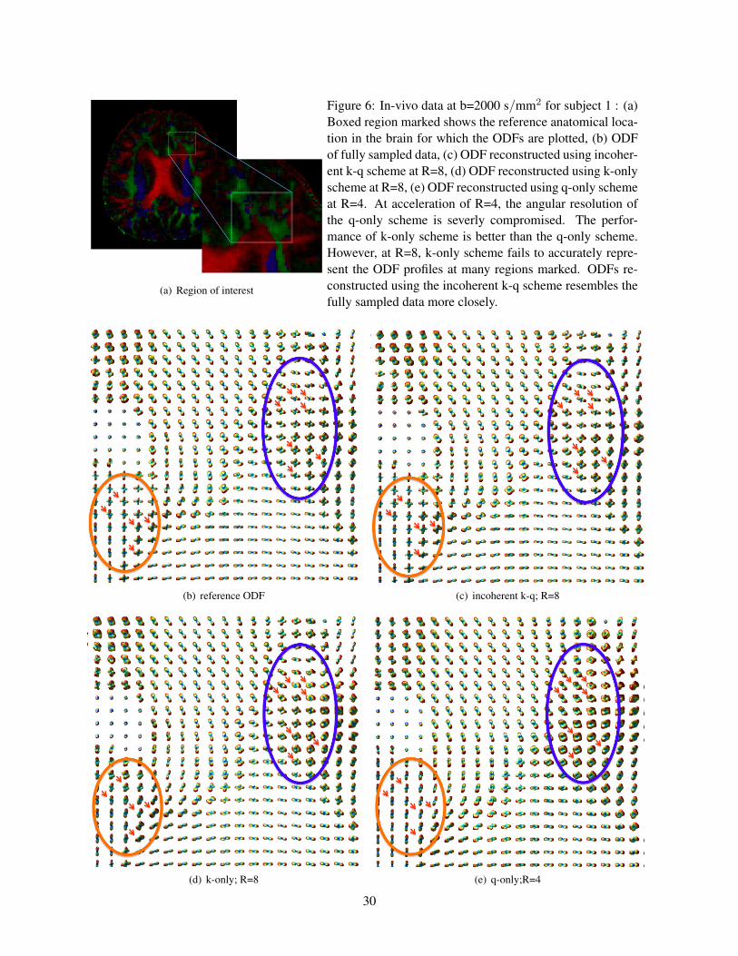
Figure 6: In-vivo data at b=2000 s/mm2 for subject 1 : (a)Boxed region marked shows the reference anatomical loca-tion in the brain for which the ODFs are plotted, (b) ODFof fully sampled data, (c) ODF reconstructed using incoher-ent k-q scheme at R=8, (d) ODF reconstructed using k-onlyscheme at R=8, (e) ODF reconstructed using q-only schemeat R=4. At acceleration of R=4, the angular resolution ofthe q-only scheme is severly compromised. The perfor-mance of k-only scheme is better than the q-only scheme.However, at R=8, k-only scheme fails to accurately repre-sent the ODF profiles at many regions marked. ODFs re-constructed using the incoherent k-q scheme resembles thefully sampled data more closely.

(b) reference ODF (c) incoherent k-q; R=8

(d) k-only; R=8 (e) q-only;R=4

30

incoherent k-q; joint k-only; two-step q-only; two-step

(a) slice #1

0 5 100

0.2

0.4

0.6

Acceleration

No

rma

lize

d O

DF

err

or

(b) Normalized ODF error

0 5 100

5

10

15

Acceleration

Ave

rag

e a

ng

ula

r e

rro

r

(c) Average Angular error

0 5 100

0.05

0.1

Acceleration

Ra

te o

f fa

lse

pe

aks

(d) Rate of False Peak

(e) slice #20 5 10

0

0.2

0.4

0.6

Acceleration

No

rma

lize

d O

DF

err

or

(f) Normalized ODF error

0 5 100

5

10

15

20

Acceleration

Ave

rag

e a

ng

ula

r e

rro

r

(g) Average Angular error

0 5 100

0.1

0.2

Acceleration

Ra

te o

f fa

lse

pe

aks

(h) Rate of False Peak

Figure 7: Plots of reconstruction errors from two different slices of subject 2 collected at b =2000 s/mm2.Slice #1 is from the superior part of corpus callosum. Slice #2 is an inferior region that is prone to pulsatilityand susceptibility effects. (b), (c) and (d) are the normalized sum of square error of the ODFs, averageangular error, and rate of false peaks respectively for the slice shown in (a). (f), (g) and (h) are the normalizedsum of square error of the ODFs, average angular error, and rate of false peaks respectively for the sliceshown in (e).

31

incoherent k-q; joint uniform k-only; jointuniform k-only; two-step incoherent k-q; two-step

Slice 9

(a) subject 1 0 5 100

0.05

0.1

Acceleration

Norm

alized O

DF

err

or

(b) Normalized ODF error

0 5 102

4

6

8

Acceleration

Ave

rag

e a

ng

ula

r e

rro

r

(c) Average Angular error

0 5 100.02

0.04

0.06

0.08

Acceleration

Rate

of fa

lse p

eaks

(d) Rate of false peaks

(e) subject 2 0 5 100

0.1

0.2

0.3

Acceleration

Norm

alized O

DF

err

or

(f) Normalized ODF error

0 5 10

4

6

8

10

Acceleration

Avera

ge a

ngula

r err

or

(g) Average Angular error

0 5 10

0.04

0.06

0.08

0.1

Acceleration

Rate

of fa

lse p

eaks

(h) Rate of false peaks

Figure 8: Plots of reconstruction errors from subject 1 and subject 2 collected at b =2000 s/mm2 usingvarious acquisition schemes. The joint optimization scheme was tested using incoherent k-q under-sampling(blue solid line) and uniform k-only under-sampling scheme (blue dotted line). Similarly, the two-stepoptimization scheme was tested using uniform k-only under-sampling scheme (red solid line) and incoherentk-q under-sampling scheme (red dotted line). Normalized ODF errors (b, f), average angular error (c, g) andrate of false peaks(d, h) are shown.

32

Table 2: Acquisition time in minutes corresponding to various acceleration schemes.Method R=1 R=2 R=4 R=8 R=11

incoherent k-q 60 30 16.25 8 5.3k-only 60 30 16.25 8 5.3

hybrid k-q; 32 dir 60 15.58 8.9hybrid k-q; 16 dir 60 8.25

q-only 60 30 15.58 8.25 6.41

33

Supplementary materialSimulated data and experiements

We create a numerical simulation data from an in-vivo human dataset that was collected at a b-value of

1200 s/mm2 with 60 diffusion directions. This data was collected using a variable density spiral trajectory

with 22 interleaves at a spatial resolution of 1mm x 1mm x 1.5 mm with an 8 channel head coil. The diffusion

images corresponding to the 60 diffusion directions were reconstructed using a SENSE reconstruction and

motion corrected. Using the model matrix A that was created for the 60 diffusion directions, the dominant

diffusion directions in each voxel of the in-vivo data were found using a matching pursuit algorithm in a

greedy fashion (1). Diffusion components were fit to the signal in each voxel until the error between the

simulated signal and the real signal were below a fixed value. Thus, the number of diffusion directions

in each voxel varied and were determined automatically based on the residual error after fitting. Once the

diffusion basis functions were obtained this way, the simulated diffusion weighted images was obtained

using the forward model in Eq. [5]. Then, k-space data corresponding to each channel and spiral interleaf

were computed for 60 diffusion directions using Eq. [8] without the motion error. Complex Gaussian noise

was added to the k-space predictions of the dataset such that the noise variance of the k-space data for each

channel and each diffusion direction matched that of the in-vivo data from which it is created. Figure 1

shows the ODF of simulated data for a small region of the brain.

To study the effect of noise on the joint and two-step reconstruction schemes, we performed the follow-

ing experiment on the simulated data. ODFs were reconstructed using the joint k-q scheme and two-step

scheme from the fully sampled data at three noise levels: (i) no noise was added, (ii) complex Gaussian

noise with half the noise variance as that of the in-vivo k-space data was added, and (iii) complex Gaussian

noise with full noise variance as that of the in-vivo k-space data was added. The reconstruction errors for

these three cases were computed and are plotted in Fig. 2. The plot shows that in the absence of noise, the

two schemes shows similar performance. However, as the noise level increase, the reconstruction error is

higher in the two-step scheme compared to the joint scheme even at no acceleration.

The effect of the various under-sampling patterns on the reconstruction scheme employed were studied

on the simulated data. Reconstructions were performed under four different settings. The simulated k-space

data was under-sampled using incoherent k-q under-sampling and reconstructed using (i) the joint recon-

struction scheme and (ii) the two-step reconstruction scheme. Similarly, the k-q data was under-sampled

using the uniform k-only under-sampling scheme and reconstructed using (i) the joint reconstruction scheme

and (ii) the two-step reconstruction scheme. The results of the these experiments are plotted in Fig. 3. It

is observed from the plots that the joint reconstruction scheme employing incoherent under-sampling of the

1

k-q space provides the best results.

2

Legends

Fig 1: Numerical data simulated from an in-vivo brain region : (a) RGB map of the in-vivo brain data from

which the simulated data was created, (b) Ground truth ODF (without noise) corresponding to the boxed

region in (a).

Fig 2: Effect of noise on reconstruction. The blue graph represents the joint reconstruction and the red graph

represents the two-step magnitude based scheme. In the absence of noise, the two schemes shows similar

performance. As noise level increases, the error in the two-step magnitude-based scheme increases because

of the inaccurate noise modeling.

Fig 3: Effect of under-sampling pattern on reconstruction. The blue graph represents the joint reconstruction

scheme that reconstructs the ODF directly from k-q data. The blue solid line represents the plots using the

incoherent k-q under-sampling pattern and the blue dotted line represents plots using the uniform k-only

under-sampling. The red graph represents the scheme that reconstructs the ODF using the two-step scheme.

The red solid line represents the plots using the uniform k-only under-sampling pattern and the red dotted

line represents plots using the incoherent k-q under-sampling pattern.

3

References

1 S. Mallat. Matching pursuits with time-frequency dictionaries. IEEE Transactions on Signal Processing, 41(12):

3397–3415, 1993. ISSN 1053587X.

4

(a) (b)

Figure 1: Numerical data simulated from an in-vivo brain region : (a) RGB map of the in-vivo brain datafrom which the simulated data was created, (b) Ground truth ODF (without noise) corresponding to theboxed region in (a).

5

incoherent k-q; joint reconstruction uniform k-only; two-step magnitude-based reconstruction

0 0.5 10.01

0.02

0.03

0.04

0.05

0.06

% Noise−level

Norm

alized O

DF

err

or

(a)

0 0.5 14

6

8

10

12

% Noise−level

Avera

ge a

ngula

r err

or

(b)

0 0.5 10.04

0.05

0.06

0.07

0.08

0.09

% Noise−level

Rate

of fa

lse p

eaks

(c)

Figure 2: Effect of noise on reconstruction. The blue graph represents the joint reconstruction and the redgraph represents the two-step magnitude based scheme. In the absence of noise, the two schemes showssimilar performance. As noise level increases, the error in the two-step magnitude-based scheme increasesbecause of the inaccurate noise modeling.

6

incoherent k-q; joint uniform k-only; jointuniform k-only; two-step incoherent k-q; two-step

4 6 8 10 120

0.05

0.1

0.15

Acceleration

Norm

alized O

DF

err

or

(a)

4 6 8 10 12

8

10

12

14

16

Acceleration

Avera

ge a

ngula

r err

or

(b)

4 6 8 10 120.05

0.1

0.15

0.2

Acceleration

Rate

of fa

lse p

eaks

(c)

Figure 3: Effect of under-sampling pattern on reconstruction. The blue graph represents the joint recon-struction scheme that reconstructs the ODF directly from k-q data. The blue solid line represents the plotsusing the incoherent k-q under-sampling pattern and the blue dotted line represents plots using the uniformk-only under-sampling. The red graph represents the scheme that reconstructs the ODF using the two-stepscheme. The red solid line represents the plots using the uniform k-only under-sampling pattern and the reddotted line represents plots using the incoherent k-q under-sampling pattern.

7

Supplementary FigureUnder-sampled Reconstruction of Non-diffusion Weighted Image for Various Accelerations

Acc= 1

(a) fully-sampledAcc= 2

(b) R=2

Acc= 4

(c) R=4

Acc= 8

(d) R=8

Acc= 11

(e) R=11Acc= 11

(f) error image for R=2

Acc= 11

(g) error image for R=4

Acc= 11

(h) error image for R=8

Acc= 11

(i) error image for R=11

Figure 4: The effect of under-sampling demonstrated on the non-diffusion weighted image collected fromdataset 2 using standard gridding reconstruction. (a) fully sampled reconstruction. (b) and (f) are the recon-struction from R=2 and its difference from the fully sampled image in (a). (c) and (g) are the reconstructionfrom R=4 and its difference from the fully sampled image in (a). (d) and (h) are the reconstruction fromR=8 and its difference from the fully sampled image in (a). (e) and (i) are the reconstruction from R=11 andits difference from the fully sampled image in (a).

8