27
Accept or Reject: Can we get the work done in time? Marjan van den Akker Joint work with Han Hoogeveen
| Date post: | 21-Dec-2015 |
| Category: |
Documents |
| View: | 214 times |
| Download: | 0 times |

Accept or Reject:
Can we get the work done in time?
Marjan van den Akker
Joint work with Han Hoogeveen

Outline of the talk
• Problem description• Review Moore-Hogdson• Stochastic processing times
– consequences– four classes of instances
• Summary
Problem setting
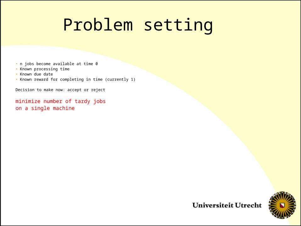
• n jobs become available at time 0• Known processing time• Known due date • Known reward for completing in time (currently 1)
Decision to make now: accept or reject
minimize number of tardy jobs on a single machine

Moore-Hodgson
1. Number the jobs in EDD order2. Let S denote the EDD schedule3. Find the first job not on time in S
(suppose this is job j)4. Remove from S the largest available
job from jobs 1,…,j5. Continue with Step 3 for this new
schedule S until all jobs are on time

Solving the problem from scratch
Observations• First the on time jobs• On time jobs in EDD order• Forget about the late jobs
Knowing the on time set is sufficient

Dominance rule
• Let E1 and E2 be two subsets of jobs 1,…,j• All jobs in E1 and E2 are on time (feasible)• Cardinality of E1 and E2 is equal• The total processing time of the jobs in E2
is more than the total processing time of the jobs in E1
Then subset E2 can be discarded.

Proof (sketch)
Take an optimal schedule starting with E2
(remainder: jobs from j+1, …, n)
E2 remainder
E1 remainder
time0

Use dynamic programming
• Find Ej*(k): feasible subset of jobs 1,…,j
with cardinality k and minimum total processing time
• Use state variables fj(k) equal to p(Ej*(k))
• Define zj as maximum number of on time jobs from jobs 1, …, j
• Initialization: fj(k)=0 for j=k=0 (and + otherwise)

Recurrence relation
• Put fj+1 (0)=0
• fj+1(k)=min{fj(k),fj(k-1)+pj+1} (k=1,…,zj)
• If fj(z_j)+pj+1 dj+1
then zj+1=zj+1 and fj+1(zj+1)=fj(zj)+pj+1; otherwise, zj+1=zj.

Relation with Moore-Hodgson
• The set Ej*(k-1) can be computed from Ej
*(k) by removing the largest job!
• Recurrence relation
fj+1(k)=min{fj(k),fj(k-1)+pj+1}
Equal to: remove the largest job

Moore-Hodgson
1. Number the jobs in EDD order2. Compute the values fj(zj):
– If fj(z_j)+pj+1 dj+1
then zj+1=zj+1 and fj+1(zj+1)=fj(zj)+pj+1
i.e. Jj+1 is added– else zj+1 = zj and
fj+1(zj+1) = min{fj(zj),fj(zj-1)+pj+1}i.e. largest job is removed

Stochastic processing times
• Completion times are uncertain
• Decision about accept or reject must be made before running the schedule
• When do you consider a job on time?

On time stochastically
• Work with a sequence of on time jobs (instead of a set of completion times)
• Add a job to this sequence and compute the probability that it is ready on time
• If this probability is large enough (at least equal to the minimum success probability msp) then accept it as on time
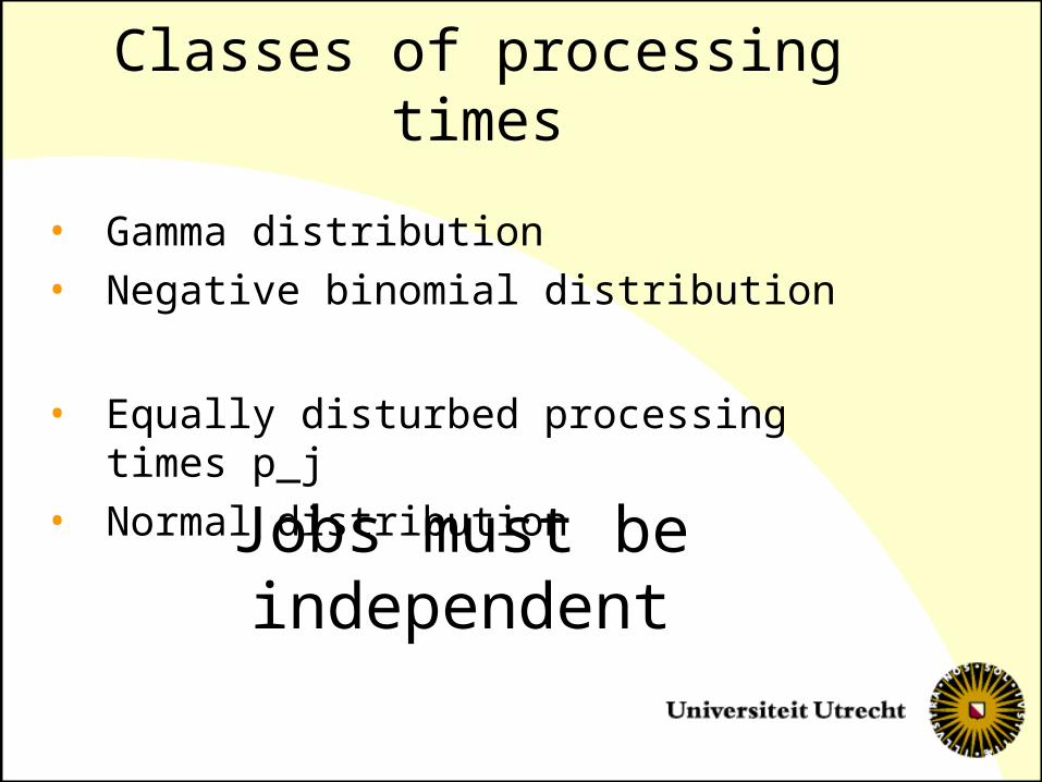
Classes of processing times
• Gamma distribution• Negative binomial distribution
• Equally disturbed processing times p_j• Normal distribution
Jobs must be independent
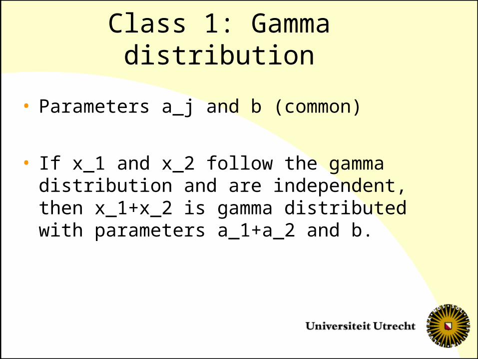
Class 1: Gamma distribution
• Parameters a_j and b (common)
• If x_1 and x_2 follow the gamma distribution and are independent, then x_1+x_2 is gamma distributed with parameters a_1+a_2 and b.

More gamma
• Define S as the set of the job j and all its predecessors in the schedule
• Define p(S) as the sum of all processing times of jobs in S
• Then C_j=p(S) follows a gamma distribution with parameters a(S) and b.

Even more gamma
• Denote the msp of job j by y_j• Job j is on time if the probability that C_j
is no more than d_j is at least y_j• C_j depends on a(S) only• Given d_j and y_j, you can compute the
maximum value of a(S) such that P(Cj <= dj) is at least yj: call it D_j

Last of Gamma
• Treat D_j as ordinary due dates• Treat a_j as ordinary deterministic
processing times• Then the dominance rule still holds
•You can use Moore-Hodgson!
• Negative binomial distribution: similar
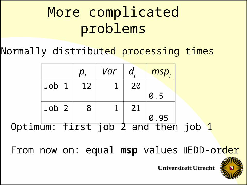
More complicated problems
pj Var dj mspj
Job 1 12 1 20 0.5
Job 2 8 1 21 0.95
Normally distributed processing times
Optimum: first job 2 and then job 1
From now on: equal msp values EDD-order

Equal disturbances• On time probability of job j depends on:
– Number of predecessors (on time jobs before j)– Total processing time of its predecessors
• Dominance rule: given the cardinality of the on time set, take the one with minimum total processing time
• Use dynamic programming with state variables fj(k) that indicate the minimum total processing possible (as before)
• Hence: Moore-Hodgson’s solves it!

Normal distribution (1)
• Parameters: expected processing time of job j and variance of job j
• Reminder: expected value and variances of X1+X2 are equal to the respective sums
• Necessary for computing the on time probability of job j:– Total processing time of predecessors– Total variance of predecessors
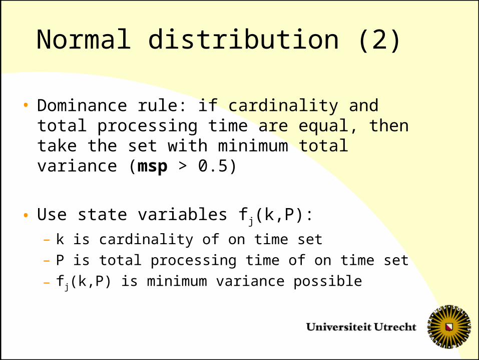
Normal distribution (2)
• Dominance rule: if cardinality and total processing time are equal, then take the set with minimum total variance (msp > 0.5)
• Use state variables fj(k,P):– k is cardinality of on time set– P is total processing time of on time set
– fj(k,P) is minimum variance possible

Normal distribution: details
• Running time pseudo-polynomial
• Problem is NP-hard
• Role of total variance and total processing time in the dominance rule and in the DP is interchangeable

What to remember (optional)
• Moore-Hodgson = Dynamic Programming
• DP is applicable in a stochastic environment– Stochastic on time: work with the minimum
success probability– EDD sequence optimal for the on time set??
• Weighted case can be solved in a similar way
Yes: single machine, minimize number of tardy jobs
Solvable in O(n log n) time byMoore-Hodgson
Known problem?

Miscellaneous remarks
• DP computes more state variables than necessary
• DP can be used for the weighted case:– Use fj(W) with W is the total weight of the on
time set (instead of cardinality of the on time set)
• DP can be used for more problems (to be shown next)
Negative binomial distribution
• Parameters s_j and p (common for all jobs)
• If independent, then C_j=p(S) follows a negative binomial distribution with parameters s(S) and p
•Same as gamma distribution


