PNNL-19315 Prepared for the U.S. Department of Energy under Contract DE-AC05-76RL01830 Acceptance Sampling Using Judgmental and Randomly Selected Samples LH Sego JE Wilson SA Shulman BA Pulsipher KK Anderson WK Sieber September 2010
Transcript
PNNL-19315
Prepared for the U.S. Department of Energy under Contract DE-AC05-76RL01830
Acceptance Sampling Using Judgmental and Randomly Selected Samples LH Sego JE Wilson SA Shulman BA Pulsipher KK Anderson WK Sieber September 2010
DISCLAIMER This report was prepared as an account of work sponsored by an agency of the United States Government. Neither the United States Government nor any agency thereof, nor Battelle Memorial Institute, nor any of their employees, makes any warranty, express or implied, or assumes any legal liability or responsibility for the accuracy, completeness, or usefulness of any information, apparatus, product, or process disclosed, or represents that its use would not infringe privately owned rights. Reference herein to any specific commercial product, process, or service by trade name, trademark, manufacturer, or otherwise does not necessarily constitute or imply its endorsement, recommendation, or favoring by the United States Government or any agency thereof, or Battelle Memorial Institute. The views and opinions of authors expressed herein do not necessarily state or reflect those of the United States Government or any agency thereof. PACIFIC NORTHWEST NATIONAL LABORATORY operated by BATTELLE for the UNITED STATES DEPARTMENT OF ENERGY under Contract DE-AC05-76RL01830 Printed in the United States of America Available to DOE and DOE contractors from the Office of Scientific and Technical Information,
email: [email protected] Available to the public from the National Technical Information Service, U.S. Department of Commerce, 5285 Port Royal Rd., Springfield, VA 22161
Acceptance Sampling Using Judgmental and Randomly Selected Samples
LH Sego1 JE Wilson
1
SA Shulman2 BA Pulsipher
1
KK Anderson1 WK Sieber
2
1. Pacific Northwest National Laboratory, Richland, WA
2. National Institute of Occupational Safety and Health, Cincinnati, OH
September 2010
Prepared for
the U.S. Department of Energy
under Contract DE-AC05-76RL01830
Pacific Northwest National Laboratory
Richland, Washington 9952
PNNL-19315
Acceptance Sampling Using Judgmental and Randomly Selected Samples
Landon H. Sego1, Stanley A. Shulman2, Kevin K. Anderson1
John E. Wilson1, Brent A. Pulsipher1, W. Karl Sieber2
September 2010
1: Statistics and Sensor Analytics Group, Pacific Northwest National Laboratory, Richland, WA2: National Institute for Occupational Safety and Health, Cincinnati, OH
Abstract
We present a Bayesian model for acceptance sampling where the population consists of two groups,
each with different levels of risk of containing unacceptable items. Expert opinion, or judgment, may
be required to distinguish between the high and low-risk groups. Hence, high-risk items are likely to
be identified (and sampled) using expert judgment, while the remaining low-risk items are sampled
randomly. We focus on the situation where all observed samples must be acceptable, where the objective
of the statistical inference is to quantify the probability that a large percentage of the unsampled items in
the population are also acceptable. We demonstrate that traditional (frequentist) acceptance sampling
and simpler Bayesian formulations of the problem are essentially special cases of the proposed model.
We explore the properties of the model in detail, and discuss the conditions necessary to ensure that the
required sample size is a non-decreasing function of the population size. The methodology is applicable
to a variety of acceptance sampling problems, including environmental sampling where the objective is
to demonstrate the safety of reoccupying a remediated facility that has been contaminated with a lethal
Because Y` ∼ Bin(N − nh − n, θh/ρ), we can then write the Bayesian confidence (1) as
C =∫ 1
0
P (Y` ≤ (1− λ)N | θh) p1(θh | Xh = 0, X` = 0) dθh
=
∫ 1
0
b(1−λ)Nc∑y=0
(N − nh − n
y
)(θh
ρ
)y (1− θh
ρ
)N−nh−n−y
p1(θh | Xh = 0, X` = 0) dθh (5)
Sample sizes can then be determined by numerically searching (5) for the smallest value of n that achieves
a desired level of confidence, C ′. This initial model was first discussed by Sego et al. (2007).
2.2 Drawbacks of the initial model
While the initial model provides a good starting point for the problem at hand, the approach has four
immediate drawbacks. First, the integrals in (4) and (5) are difficult to accurately calculate with standard
numerical integration routines because their integrands are mostly constant (near 0) over the unit interval.
This is especially true for large values of β. Second, defining θh = ρθ` results in truncating the support of
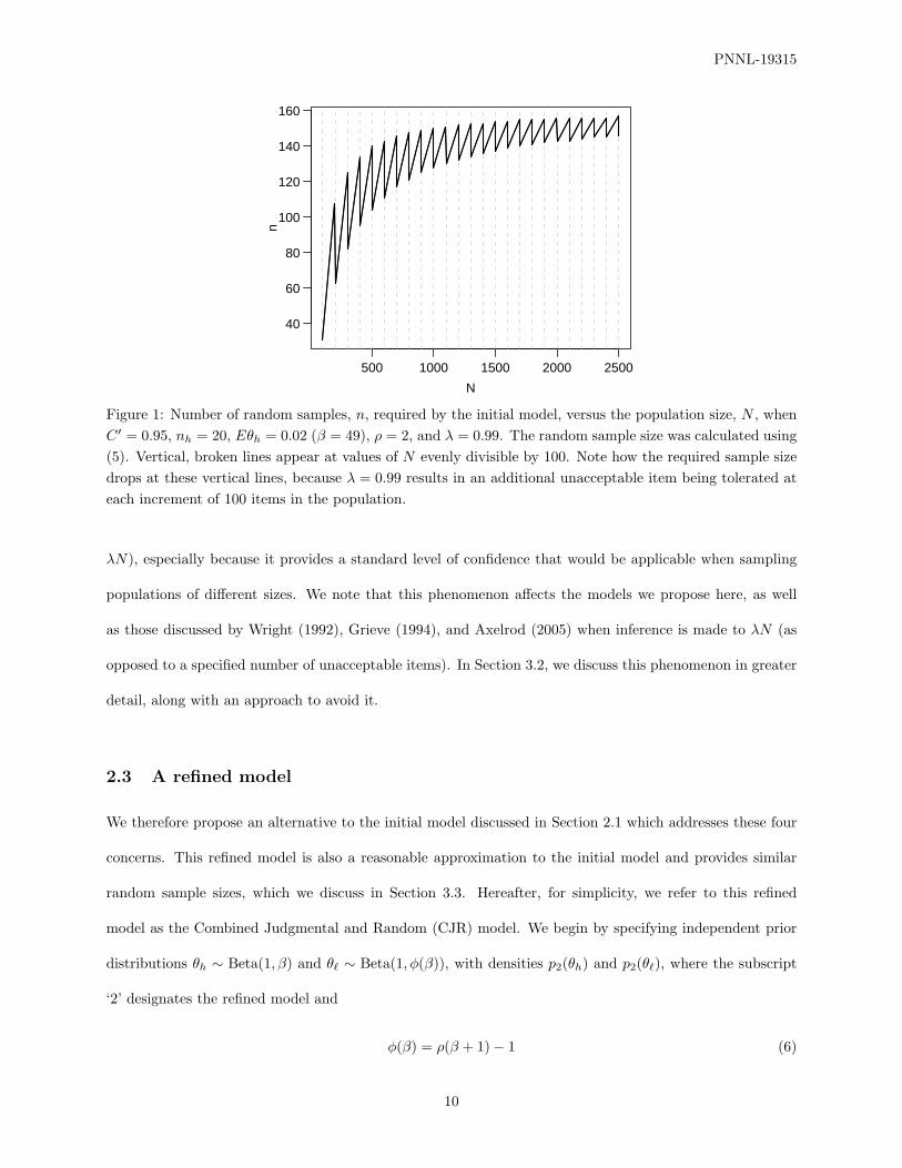
the prior distribution of θ` to (0, 1/ρ), which may not be desirable. Third, because the distribution function
of Y` is discrete, the required sample size can oscillate strongly for increasing values of N , as illustrated in
Figure 1.
Fourth, in situations where the prior evidence is strong (i.e. which is reflected in large values of β and/or
ρ) relative to the desired fraction of acceptability, λ, the confidence function (5) is not necessarily a decreasing
function of N . The practical implication is that more samples may be required for a smaller population than
for a larger population to achieve the same level of confidence—an undesirable and non-intuitive result. This
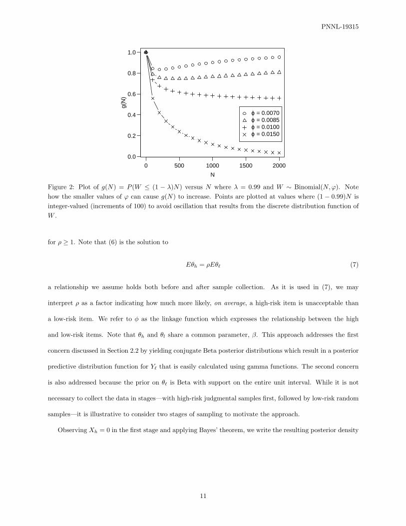
phenomenon results from an interesting characteristic of the binomial distribution function. To illustrate,
let g(N) = P (W ≤ (1 − λ)N) for W ∼ Binomial(N, ϕ). Then, for values of ϕ that are small relative to
1− λ, we observe g(N) is not a decreasing function of N . However, larger values of ϕ result in a decreasing
function of g. This phenomenon is illustrated in Figure 2. One of the factors that induces this phenomenon
is the dependence of the distribution of W on N . Thus, one way to avoid it would be to make inference to a
specific number of unacceptable items, rather than a fraction of the population size. For example, we could
desire a high probability that no more than, say, 10 items in the population be unacceptable. Nonetheless,
in many applications, it is often desirable to make inference to a quantile of the population (in this case,
9
PNNL-19315
500 1000 1500 2000 2500
40
60
80
100
120
140
160
N
n
Figure 1: Number of random samples, n, required by the initial model, versus the population size, N , whenC ′ = 0.95, nh = 20, Eθh = 0.02 (β = 49), ρ = 2, and λ = 0.99. The random sample size was calculated using(5). Vertical, broken lines appear at values of N evenly divisible by 100. Note how the required sample sizedrops at these vertical lines, because λ = 0.99 results in an additional unacceptable item being tolerated ateach increment of 100 items in the population.
λN), especially because it provides a standard level of confidence that would be applicable when sampling
populations of different sizes. We note that this phenomenon affects the models we propose here, as well
as those discussed by Wright (1992), Grieve (1994), and Axelrod (2005) when inference is made to λN (as
opposed to a specified number of unacceptable items). In Section 3.2, we discuss this phenomenon in greater
detail, along with an approach to avoid it.
2.3 A refined model
We therefore propose an alternative to the initial model discussed in Section 2.1 which addresses these four
concerns. This refined model is also a reasonable approximation to the initial model and provides similar
random sample sizes, which we discuss in Section 3.3. Hereafter, for simplicity, we refer to this refined
model as the Combined Judgmental and Random (CJR) model. We begin by specifying independent prior
distributions θh ∼ Beta(1, β) and θ` ∼ Beta(1, φ(β)), with densities p2(θh) and p2(θ`), where the subscript
‘2’ designates the refined model and
φ(β) = ρ(β + 1)− 1 (6)
10
PNNL-19315
0 500 1000 1500 2000
0.0
0.2
0.4
0.6
0.8
1.0
N
g(N
)
ϕ = 0.0070 ϕ = 0.0085 ϕ = 0.0100 ϕ = 0.0150
Figure 2: Plot of g(N) = P (W ≤ (1 − λ)N) versus N where λ = 0.99 and W ∼ Binomial(N,ϕ). Notehow the smaller values of ϕ can cause g(N) to increase. Points are plotted at values where (1 − 0.99)N isinteger-valued (increments of 100) to avoid oscillation that results from the discrete distribution function ofW .
for ρ ≥ 1. Note that (6) is the solution to
Eθh = ρEθ` (7)
a relationship we assume holds both before and after sample collection. As it is used in (7), we may
interpret ρ as a factor indicating how much more likely, on average, a high-risk item is unacceptable than
a low-risk item. We refer to φ as the linkage function which expresses the relationship between the high
and low-risk items. Note that θh and θl share a common parameter, β. This approach addresses the first
concern discussed in Section 2.2 by yielding conjugate Beta posterior distributions which result in a posterior
predictive distribution function for Y` that is easily calculated using gamma functions. The second concern
is also addressed because the prior on θ` is Beta with support on the entire unit interval. While it is not
necessary to collect the data in stages—with high-risk judgmental samples first, followed by low-risk random
samples—it is illustrative to consider two stages of sampling to motivate the approach.
Observing Xh = 0 in the first stage and applying Bayes’ theorem, we write the resulting posterior density
11
PNNL-19315
of θh without the constant of integration, where f denotes the binomial likelihood:
p2(θh | Xh = 0) ∝ p2(θh)f(Xh = 0 | θh)
∝ (1− θh)β−1(1− θh)nh (8)
= (1− θh)nh+β−1
which gives the well-known (Gelman et al., 2004) conjugate posterior of θh|(Xh = 0) ∼ Beta(1, nh +β). The
information obtained by observing Xh = 0 is reflected in the updated value of the shape parameter: nh + β.
By inserting this updated value into the prior on θl, we allow the outcome of Xh = 0 to increase our prior
belief in the acceptability of the low-risk samples. Therefore, substituting the updated shape parameter into
the prior for θl via (6) gives
θ` ∼ Beta(1, φ(nh + β)) (9)
We abuse the conditioning notation and denote this updated prior density of θ` as p2(θ` | Xh = 0) to reflect
the information obtained by the nh acceptable judgmental items. Alternatively, we could view the first stage
sampling of the high-risk items as an approach to elicit the prior distribution for θ` before sampling the
low-risk group.
Upon observing X` = 0 in the second stage, we arrive at the posterior distribution for θ` by combining
the binomial likelihood of n acceptable low-risk items with the updated prior, p2(θ` | Xh = 0), in a manner
similar to (8). This gives θ`|(Xh = 0, X` = 0) ∼ Beta(1, β′) where
β′ := n + φ(nh + β) = n + ρ(nh + β + 1)− 1 (10)
Note that β′ has a natural interpretation: the nh acceptable, judgmentally sampled items are weighted ρ
times more than the n acceptable, randomly sampled items.
Having observed Xh = 0 and X` = 0, the number of low-risk, unsampled items which are unacceptable,
Y`, is Binomial with N − nh − n trials and probability θ`|(Xh = 0, X` = 0). Letting FY`(y | θ`) denote the
where Ψ(x) = ddx log Γ(x) is the digamma function. Because log Γ(x) is convex, Ψ(x) is increasing, which
implies Ψ(A3)−Ψ(A1) < 0 and (ρ− 1) (Ψ(A2)−Ψ(A4)) ≤ 0. This, combined with the fact that 0 ≤ h ≤ 1,
implies that ∂h∂nh
≥ 0 over P. In like manner, it is straightforward to show that ∂h∂n ≥ 0, ∂h
∂ρ ≥ 0, ∂h∂β ≥ 0,
and ∂h∂λ ≤ 0, also over P. These results are consistent with how we would expect the confidence function to
behave. However, the behavior of h(N) is not consistently increasing or decreasing, due to the characteristics
of the binomial distribution function discussed in Section 2.2 and illustrated in Figures 2 and 3. Note that
the partial derivative of h with respect to N is
∂h
∂N= (h− 1) (Ψ(A1) + λΨ(A2)− λΨ(A3)−Ψ(A4)) (25)
15
PNNL-19315
For λ = 1, we can apply the recurrence relation, Ψ(x+1) = Ψ(x)+1/x, (Abramowitz and Stegun, 1972, eq.
6.3.5) to show
∂h
∂N= (h− 1)
(Ψ(A3) +
1A3
−Ψ(A3) + Ψ(A2)−Ψ(A2)− 1A2
)
= (h− 1)(
1N − nh − n
− 1N + nh(ρ− 1) + ρ(β + 1)− 1
)≤ 0 (26)
over the subset of P induced by λ = 1. This finding is intuitive: given the same prior belief (reflected by
β), the same number of acceptable samples nh and n, and the same ρ, we would expect, for a population of
size 100, the confidence that 100% of the items being acceptable should be greater than for a population of
one million items. However, for λ < 1, the behavior of h(N) depends upon other variables in the parameter
space, P, and in particular, it is most sensitive to β.
C
0.94
0.95
0.96
0.97
0.98
0.99
β = 125 β = 175 β = 225 β = 250
(A)
N
n
0 200 400 600 800 1000
0
25
50
75
100
125
150(B)
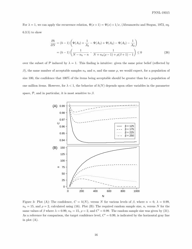
Figure 3: Plot (A): The confidence, C = h(N), versus N for various levels of β, where n = 0, λ = 0.99,nh = 15, and ρ = 2, calculated using (16). Plot (B): The required random sample size, n, versus N for thesame values of β where λ = 0.99, nh = 15, ρ = 2, and C ′ = 0.99. The random sample size was given by (21).As a reference for comparison, the target confidence level, C ′ = 0.99, is indicated by the horizontal gray linein plot (A).
16
PNNL-19315
Figure 3A demonstrates the influence of β on h(N) when no random samples are taken (n = 0). Figure
3B shows how the required sample size, n, varies as a function of N , with a desired confidence of C ′ = 0.99,
for the same values of λ, β, nh, and ρ as in Figure 3A. Note how the curves in the two plots are somewhat
reflective of each other. In particular, notice in Figure 3B how n can actually decrease as N increases for
higher values of β, a non-intuitive and undesirable result. This undesirable behavior in h(N) is likely to
occur when the posterior expectation of the fraction of acceptable items is too large relative to λ. This
typically occurs when the prior belief in the acceptability of the high-risk items is high (corresponding to
large values of β), and/or when ρ is large. It is illustrative to consider that before any samples are taken,
our prior belief in the fraction of the population that is acceptable, λp, is determined by β, nh, ρ, and N .
Specifically,
λp = E
(1− Xh + X` + Y`
N
)= 1− N + nh(ρ− 1)
Nρ(β + 1)(27)
Details of the derivation of (27) are provided in Appendix D. When λp is too large relative to λ, the
prior belief, in a sense, already satisfies the intent to demonstrate (through sampling) that λ× 100% of the
population is acceptable. Hence, it is not surprising that large values of λp (relative to λ) are likely to result
in undesirable behavior in h(N).
3.2 Ensuring the Bayesian confidence is a non-increasing function of the popu-
lation size
Because h(n) is increasing, it follows that when h(N, n = 0) is decreasing, the number of random samples
given by (21) will be an increasing function of N . Consequently, choosing a ‘viable’ value of λ large enough
to ensure that h(N) is non-increasing will also ensure that, all things being equal, larger populations will
require more samples than smaller populations. This viable value of the fraction of acceptable items, λv,
could then be used to calculate the desired random sample size, n. The way in which λ influences the shape
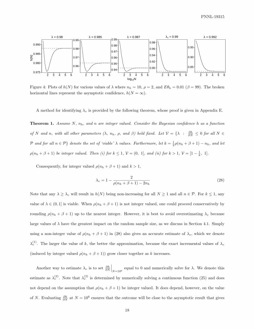
of the confidence function is illustrated in Figure 4. Note how increasing the value of λ improves the profile
of h(N) until, at λv = 0.99, it is a non-decreasing function of N . Furthermore, for λ = 0.992, (in fact, for
all λ ≥ 0.99), h(N) is also non-increasing.
17
PNNL-19315
h(N
)
λ = 0.98
0.975
0.980
0.985
0.990
2 3 4 5 6
λ = 0.985
0.96
0.97
0.98
0.99
2 3 4 5 6
λ = 0.987
0.94
0.95
0.96
0.97
0.98
0.99
2 3 4 5 6
λν = 0.99
0.90
0.92
0.94
0.96
0.98
2 3 4 5 6
λ = 0.992
0.85
0.90
0.95
2 3 4 5 6log10N
Figure 4: Plots of h(N) for various values of λ where nh = 10, ρ = 2, and Eθh = 0.01 (β = 99). The brokenhorizontal lines represent the asymptotic confidence, h(N = ∞).
A method for identifying λv is provided by the following theorem, whose proof is given in Appendix E.
Theorem 1. Assume N , nh, and n are integer valued. Consider the Bayesian confidence h as a function
of N and n, with all other parameters (λ, nh, ρ, and β) held fixed. Let V = {λ : ∂h∂N ≤ 0 for all N ∈
P and for all n ∈ P} denote the set of ‘viable’ λ values. Furthermore, let k = 12ρ(nh + β + 1)− nh, and let
ρ(nh + β + 1) be integer valued. Then (i) for k ≤ 1, V = (0, 1], and (ii) for k > 1, V = [1− 1k , 1].
Consequently, for integer valued ρ(nh + β + 1) and k > 1,
λv = 1− 2ρ(nh + β + 1)− 2nh
(28)
Note that any λ ≥ λv will result in h(N) being non-increasing for all N ≥ 1 and all n ∈ P. For k ≤ 1, any
value of λ ∈ (0, 1] is viable. When ρ(nh + β + 1) is not integer valued, one could proceed conservatively by
rounding ρ(nh + β + 1) up to the nearest integer. However, it is best to avoid overestimating λv because
large values of λ have the greatest impact on the random sample size, as we discuss in Section 4.1. Simply
using a non-integer value of ρ(nh + β + 1) in (28) also gives an accurate estimate of λv, which we denote
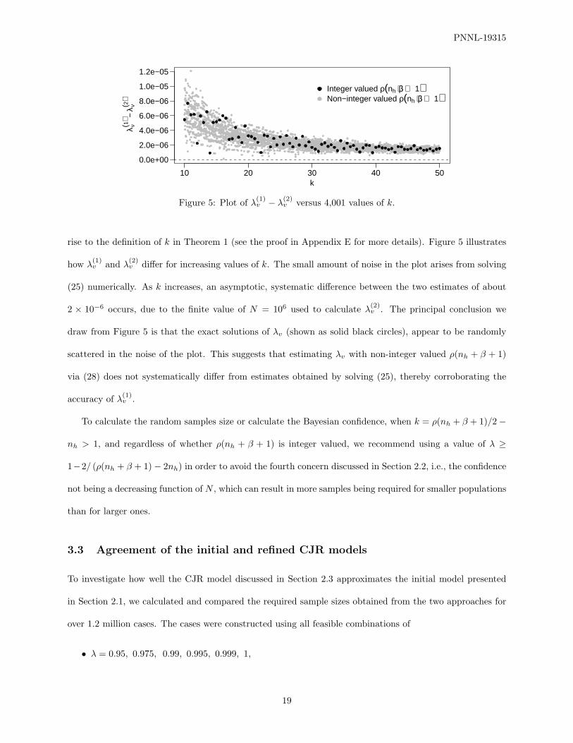
λ(1)v . The larger the value of k, the better the approximation, because the exact incremental values of λv
(induced by integer valued ρ(nh + β + 1)) grow closer together as k increases.
Another way to estimate λv is to set ∂h∂N
∣∣∣N=106
equal to 0 and numerically solve for λ. We denote this
estimate as λ(2)v . Note that λ
(2)v is determined by numerically solving a continuous function (25) and does
not depend on the assumption that ρ(nh + β + 1) be integer valued. It does depend, however, on the value
of N . Evaluating ∂h∂N at N = 106 ensures that the outcome will be close to the asymptotic result that gives
• eight values of nh: 0, 10, 25, 50, 100, 250, 500, and 750. When ρ = 1, there is no distinction between
the high and low risk locations, and thus nh was set to 0 for those cases.
The values of N and λ were chosen so that (1−λ)N would be integer valued, thus ensuring that FY`= F ?
Y`.
For these cases, we did not use λv to calculate the sample sizes because it would have made it considerably
more difficult to ensure that (1 − λ)N was integer valued. However, simply using the six values of λ listed
above still allowed us to compare how the confidence functions given by (5) and (14) give rise to the required
random sample sizes.
For each of these cases, the random sample size given by the initial model, nInit, was obtained by
identifying the value of n such that the Bayesian confidence given by (5) was at least as great as C ′. For the
approximation approach of Section 2.3, the random sample size, nCJR, was obtained from (22) when λ = 1,
from (23) when N > 106, and from (21) for the rest (and vast majority) of the cases that were considered.
For roughly 70% of these cases, nInit and nCJR were both 0, indicating that prior belief represented by Eθh
and ρ combined with the outcomes from the nh acceptable judgmental samples provided sufficient evidence
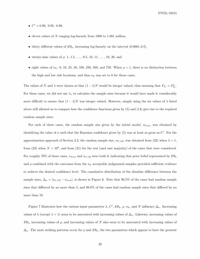
to achieve the desired confidence level. The cumulative distribution of the absolute difference between the
sample sizes, ∆n = |nCJR − nInit|, is shown in Figure 6. Note that 96.5% of the cases had random sample
sizes that differred by no more than 5, and 98.6% of the cases had random sample sizes that differed by no
more than 10.
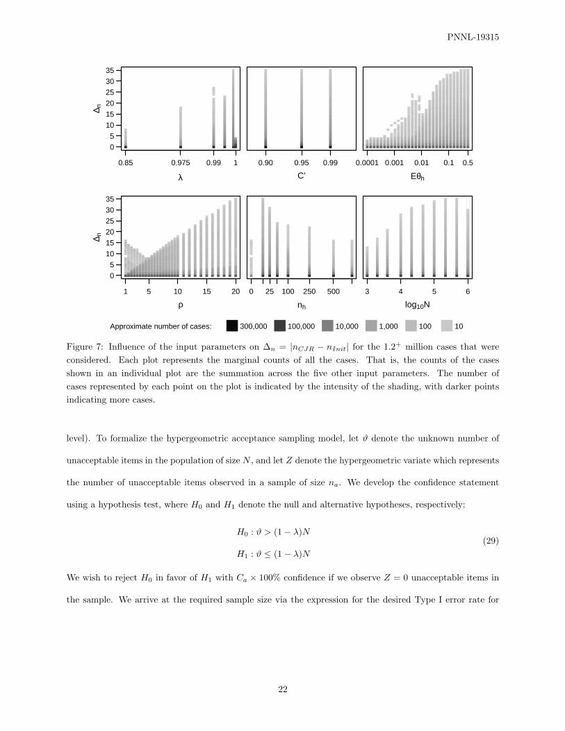
Figure 7 illustrates how the various input parameters λ, C ′, Eθh, ρ, nh, and N influence ∆n. Increasing
values of λ (except λ = 1) seem to be associated with increasing values of ∆n. Likewise, increasing values of
Eθh, increasing values of ρ, and increasing values of N also seem to be associated with increasing values of
∆n. The most striking patterns occur for ρ and Eθh, the two parameters which appear to have the greatest
20
PNNL-19315
0 10 20 30
0.80
0.85
0.90
0.95
1.00
Fra
ctio
n of
cas
es≤
∆ n
∆n = |nCJR − nInit|
Figure 6: Cumulative distribution of the absolute difference between the random sample sizes required bythe initial model discussed in Section 2.1 and the refined CJR model discussed in Section 2.3.
influence on the shape of the posterior distribution θ`|(Xh = 0, X` = 0).
For practical purposes, the refined model and the initial model behave very similarly in terms of the
required random sample size, especially for smaller values of Eθh and smaller values of ρ. However, the
refined CJR model has desirable properties that eliminate the four drawbacks of the initial model which are
discussed in Section 2.2.
3.4 Comparison to traditional acceptance sampling
Traditional acceptance sampling based on the hypergeometric or binomial distributions is discussed by
(Schilling and Neubauer, 2009) and (Bowen and Bennett, 1988). This frequentist approach was designed
for homogeneous populations and makes no prior assumptions regarding the fraction of unacceptable items.
Using the hypergeometric distribution to model the number of unacceptable items in the population, we can
identify the smallest sample size such that the probability of observing zero unacceptable items, given that
at least λ× 100% of the items are acceptable, is at least as large as a given confidence threshold, Ca. While
certainly not equivalent, Ca is the conceptual analog of the Bayesian probability, C, given by (1). We present
this methodology in a way that differs somewhat from the explanation given by Bowen and Bennett (1988),
whose approach is slightly conservative (resulting in an achieved confidence that is higher than the desired
21
PNNL-19315
λ
∆ n
0
5
10
15
20
25
30
35
0.85 0.975 0.99 1
C’
0.90 0.95 0.99
Eθh
0.0001 0.001 0.01 0.1 0.5
ρ
∆ n
0
5
10
15
20
25
30
35
1 5 10 15 20
nh
0 25 100 250 500
log10N
3 4 5 6
Approximate number of cases: 300,000 100,000 10,000 1,000 100 10
Figure 7: Influence of the input parameters on ∆n = |nCJR − nInit| for the 1.2+ million cases that wereconsidered. Each plot represents the marginal counts of all the cases. That is, the counts of the casesshown in an individual plot are the summation across the five other input parameters. The number ofcases represented by each point on the plot is indicated by the intensity of the shading, with darker pointsindicating more cases.
level). To formalize the hypergeometric acceptance sampling model, let ϑ denote the unknown number of
unacceptable items in the population of size N , and let Z denote the hypergeometric variate which represents
the number of unacceptable items observed in a sample of size na. We develop the confidence statement
using a hypothesis test, where H0 and H1 denote the null and alternative hypotheses, respectively:
H0 : ϑ > (1− λ)N
H1 : ϑ ≤ (1− λ)N(29)
We wish to reject H0 in favor of H1 with Ca × 100% confidence if we observe Z = 0 unacceptable items in
the sample. We arrive at the required sample size via the expression for the desired Type I error rate for
22
PNNL-19315
this test:
1− Ca ≥ P (Reject H0 | H0 is true)
= P (Z = 0 | ϑ > (1− λ)N) (30)
≥ P (Z = 0 | ϑ = ϑ0)
where ϑ0 = b(1 − λ)Nc + 1 denotes the smallest whole number of unacceptable items that may be in the
population if H0 is true. Rewriting the last line in (30) using the mass function of Z, we have
1− Ca ≥
(ϑ0
0
)(N − ϑ0
na − 0
)
(N
na
) =(N − ϑ0)! (N − na)!(N − ϑ0 − na)! N !
(31)
and thus the sample size is the smallest na which satisfies (31). Jaech (1973, pp 327) provided a convenient
approximation for the mass function of Z evaluated at 0:
P (Z = 0 | ϑ = ϑ0) =(N − ϑ0)! (N − na)!(N − ϑ0 − na)! N !
≈(
1− 2na
2N − ϑ0 + 1
)ϑ0
(32)
which, when solved for na, gives
na = d0.5(1− (1− Ca)1/ϑ0)(2N − ϑ0 + 1)e (33)
The CJR method (when the population is assumed to be homogeneous and a non-informative prior is
used) requires virtually identical sample sizes as those required by the hypergeometric acceptance sampling
(AS) method. This is illustrated in Table 1, which gives the number of random samples required to achieve
a 95% probability (for the CJR method) or 95% confidence (for the AS method) that a high percentage
(95% or 99%) of the items in the population are acceptable. Sample sizes for the CJR model were calculated
using (21), with β = 1 (a uniform prior), nh = 0, and ρ = 1. For each of the CJR cases shown in Table 1,
the values of λ = 0.95 and 0.90 were viable, because k = 1 for these cases. Sample sizes for the AS approach
were calculated using (33), which, for the cases we tried, proved to be identical to samples sizes given by
solving (31).
Given the similarity in their sample sizes, it is not surprising that the confidence functions of the CJR
and AS models are also closely related. If we assume λN is a whole number, ϑ0 = N − λN + 1, and we can
write (31) as
Ca = 1− (λN − 1)! (N − na)!(λN − na − 1)! N !
= 1− Γ(λN) Γ(N − na + 1)Γ(λN − na) Γ(N + 1)
(34)
23
PNNL-19315
λ = 0.95 λ = 0.99N CJR AS CJR AS
100 38 39 78 781,000 55 56 237 238
10,000 58 59 290 291100,000 58 59 297 298
Table 1: Sample sizes required by the CJR method and the hypergeometric acceptance sampling (AS)method for C ′ = Ca = 0.95. For the CJR, nh = 0, Eθh = 0.5 (β = 1), and ρ = 1.
which bears a close resemblance to (14) when nh = 0, ρ = 1, and β = 1:
C = 1− Γ(λN + 1) Γ(N − n + 1)Γ(λN − n) Γ(N + 2)
= 1− λN
N + 1
[Γ(λN) Γ(N − n + 1)Γ(λN − n) Γ(N + 1)
](35)
and thus 1− C and 1− Ca differ only by a factor of λN/(N + 1).
4 Discussion
4.1 Why requiring “100% acceptable” is not acceptable
Certainly it is most desirable to state with high probability that the population has no unacceptable items,
i.e. λ = 1. However, achieving that degree of certainty typically requires that almost the entire population
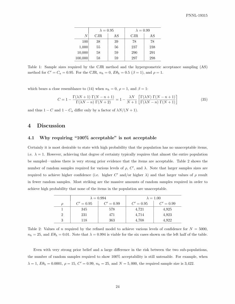
be sampled—unless there is very strong prior evidence that the items are acceptable. Table 2 shows the
number of random samples required for various levels of ρ, C ′, and λ. Note that larger samples sizes are
required to achieve higher confidence (i.e. higher C ′ and/or higher λ) and that larger values of ρ result
in fewer random samples. Most striking are the massive amounts of random samples required in order to
achieve high probability that none of the items in the population are unacceptable.
λ = 0.994 λ = 1.00ρ C ′ = 0.95 C ′ = 0.99 C ′ = 0.95 C ′ = 0.991 345 578 4,721 4,9252 231 471 4,714 4,9233 118 363 4,708 4,922
Table 2: Values of n required by the refined model to achieve various levels of confidence for N = 5000,nh = 25, and Eθh = 0.01. Note that λ = 0.994 is viable for the six cases shown on the left half of the table.
Even with very strong prior belief and a large difference in the risk between the two sub-populations,
the number of random samples required to show 100% acceptability is still untenable. For example, when
λ = 1, Eθh = 0.0001, ρ = 15, C ′ = 0.99, nh = 25, and N = 5, 000, the required sample size is 3,422.
24
PNNL-19315
λ
0.990 0.992 0.994 0.996 0.998 1.000
0
1000
2000
3000
4000
n
ρ = 2ρ = 3ρ = 4
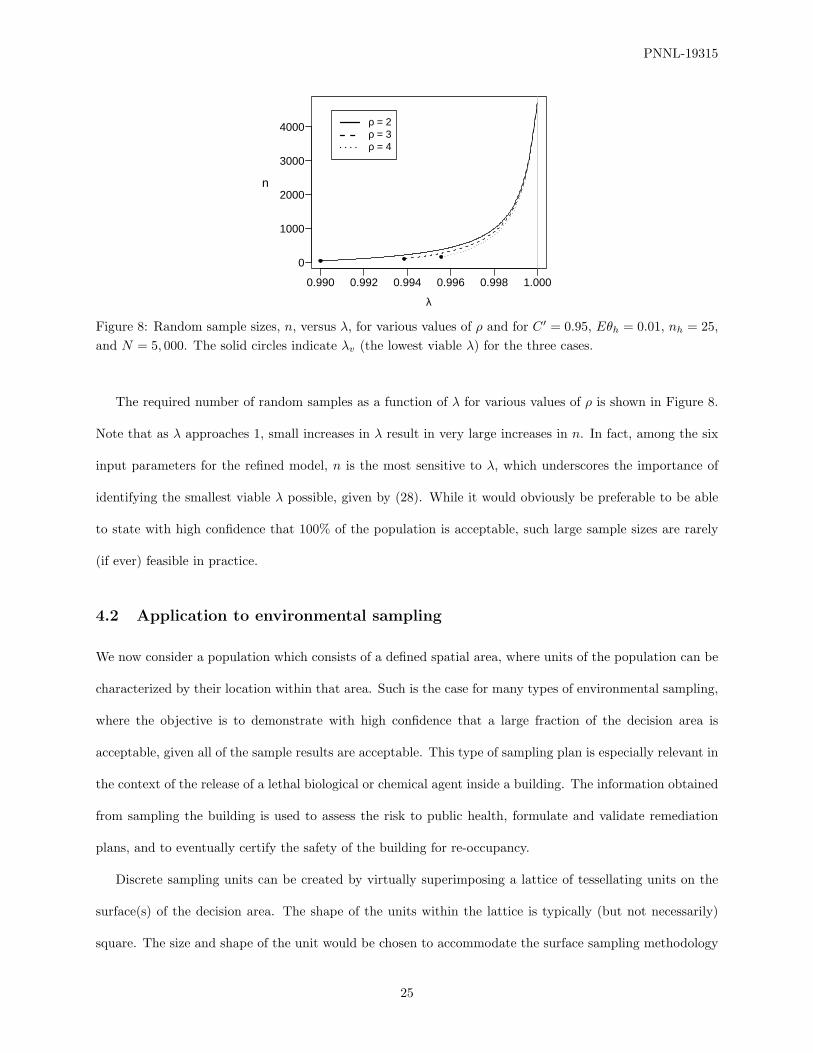
Figure 8: Random sample sizes, n, versus λ, for various values of ρ and for C ′ = 0.95, Eθh = 0.01, nh = 25,and N = 5, 000. The solid circles indicate λv (the lowest viable λ) for the three cases.
The required number of random samples as a function of λ for various values of ρ is shown in Figure 8.
Note that as λ approaches 1, small increases in λ result in very large increases in n. In fact, among the six
input parameters for the refined model, n is the most sensitive to λ, which underscores the importance of
identifying the smallest viable λ possible, given by (28). While it would obviously be preferable to be able
to state with high confidence that 100% of the population is acceptable, such large sample sizes are rarely
(if ever) feasible in practice.
4.2 Application to environmental sampling
We now consider a population which consists of a defined spatial area, where units of the population can be
characterized by their location within that area. Such is the case for many types of environmental sampling,
where the objective is to demonstrate with high confidence that a large fraction of the decision area is
acceptable, given all of the sample results are acceptable. This type of sampling plan is especially relevant in
the context of the release of a lethal biological or chemical agent inside a building. The information obtained
from sampling the building is used to assess the risk to public health, formulate and validate remediation
plans, and to eventually certify the safety of the building for re-occupancy.
Discrete sampling units can be created by virtually superimposing a lattice of tessellating units on the
surface(s) of the decision area. The shape of the units within the lattice is typically (but not necessarily)
square. The size and shape of the unit would be chosen to accommodate the surface sampling methodology
25
PNNL-19315
(Emanuel et al., 2008, Ch. 5). In practice, sample locations are often chosen from the units of the lattice based
on professional judgment from areas presumed most likely to be contaminated. For example, investigators at
the National Institute of Occupational Safety and Health (NIOSH) successfully used professional judgment
approaches to quickly identify the presence of Bacillus anthracis contamination during the 2001 anthrax
incidents. However, decisions that are based solely upon the results of judgmental samples rely heavily on
the accuracy of the professional judgment.
To achieve greater confidence that a decision area is acceptable, it is desirable to augment judgmental
samples with samples that are taken from randomly selected locations. Hence, judgmental samples are
presumed to come from the high-risk sub-population, whereas randomly selected samples are presumed to
come from the low-risk sub-population. The initial model and refined CJR model presented in Sections
2.1 and 2.3 were originally developed for this type of environmental sampling. We envision that the CJR
model would be especially applicable in situations where it is necessary to demonstrate the acceptability of a
decision area, but there is little reason to expect the presence of contamination—either because the decision
area is well-removed from the source of contamination, or perhaps because the area has been decontaminated.
We generally expect that data obtained from environmental sampling may exhibit spatial correlation,
where samples from locations that are proximal to one another exhibit higher positive correlation than those
that are separated by larger distances. If the structure of this correlation were known before sampling, it
could be used to potentially reduce the required number of acceptable random samples. More precisely, if
a sampled unit proves to be acceptable, it may be likely that adjacent units would also be acceptable, with
the positive correlation diminishing for units that are further away. Consequently, in a well-defined spatial
model, accounting for the correlation would reduce the risk for unsampled units that are proximal to the
acceptable, sampled locations, thereby increasing the overall confidence and reducing the required number
of random samples.
The CJR model does not account for spatial correlation, as all items (or units) in the population are
modeled as independent Bernoulli observations. Not accounting for spatial variability is conservative and
results in larger sample sizes than we would expect if some type of spatial correlation model were assumed for
the decision area. Because the inference made via the CJR model is conditional on observing no unacceptable
26
PNNL-19315
items, modeling the structure of the spatial correlation (Cressie, 1993) from such data would be impossible,
and a spatial model would have to be inferred from other information, if it were available. Furthermore, in
cases when sampling is conducted to validate remediation efforts, the impact of the decontamination process
on the spatial correlation is likely to be unknown (or unknowable)—in which case a sampling design that
does not rely on the estimates of spatial correlation, such as the CJR model, would be appropriate.
4.3 Recommendations for practitioners
Sego et al. (2007) presents the initial model (from Section 2.1) in the context of environmental sampling, with
additional background and explanations that may be helpful to those less familiar with statistical models.
The CJR model is based on binary outcomes, such as 1) the presence or absence of a particular quality, 2)
a quantitative sample result being acceptable or unacceptable as defined by an action level threshold or the
limit of detection, 3) contamination being detected or not detected, etc. Consequently, it is important to
clearly define the criterion whereby sample outcomes will be labeled ‘acceptable’ or ‘unacceptable.’
In addition to choosing the desired confidence level (C ′ and λ), there are two parameters that must be
specified by the investigator before sampling begins. The first is Eθh, the expected rate of unacceptable
items in the high-risk sub-population. The second is ρ, the factor that indicates the ratio of the expected
probability of an unacceptable judgmental sample to the expected probability of an unacceptable random
sample.
In general, we recommend using values of Eθh between 0.001 and 0.5. If the investigator prefers to make a
neutral (non-informative) assertion regarding the prior belief on θh, setting Eθh = 0.5 results in the uniform
prior. However, for acceptance sampling, the uniform prior is very conservative (and even pessimistic)
because it essentially represents a prior belief where “the chance of a high-risk item being unacceptable is
1%” is just as likely as “the chance of a high-risk item being unacceptable is 99%.”
We recommend that ρ be chosen conservatively, so that investigators err on the side of underestimating
ρ. However, overly conservative estimates can result in large numbers of random samples required to obtain
the desired confidence level. In general, we recommend choosing values of ρ between 1 and 5. Choosing
a value of ρ = 1 makes the contribution of the judgmental samples equivalent to the random samples, in
27
PNNL-19315
which case we recommend setting nh = 0. This ensures that the formulas presented in Section 2.3 collapse
to remove the distinction between θh and θ`, thereby modeling a homogeneous population. Consequently,
the prior would be elicited by specifying the fraction of the population that we expect to be unacceptable
prior to sampling, and this value would be used in place of Eθh in (2).
nh=10
ρ
0 0.8 0.9
0.95 0.975
0.99
0.995
0.9975
0.999
0.9995
1 2 3 4 5
0.5
0.2
0.1
0.05
0.020.01
0.005
0.0020.001
Eθ h
nh=50
ρ 0 0.9 0.95
0.975 0.983
0.99 0.995
0.9975
0.999
0.9995
1 2 3 4 5
nh=100
ρ
0 0.95 0.975
0.99 0.993
0.995
0.9975
0.999
0.9995
1 2 3 4 5
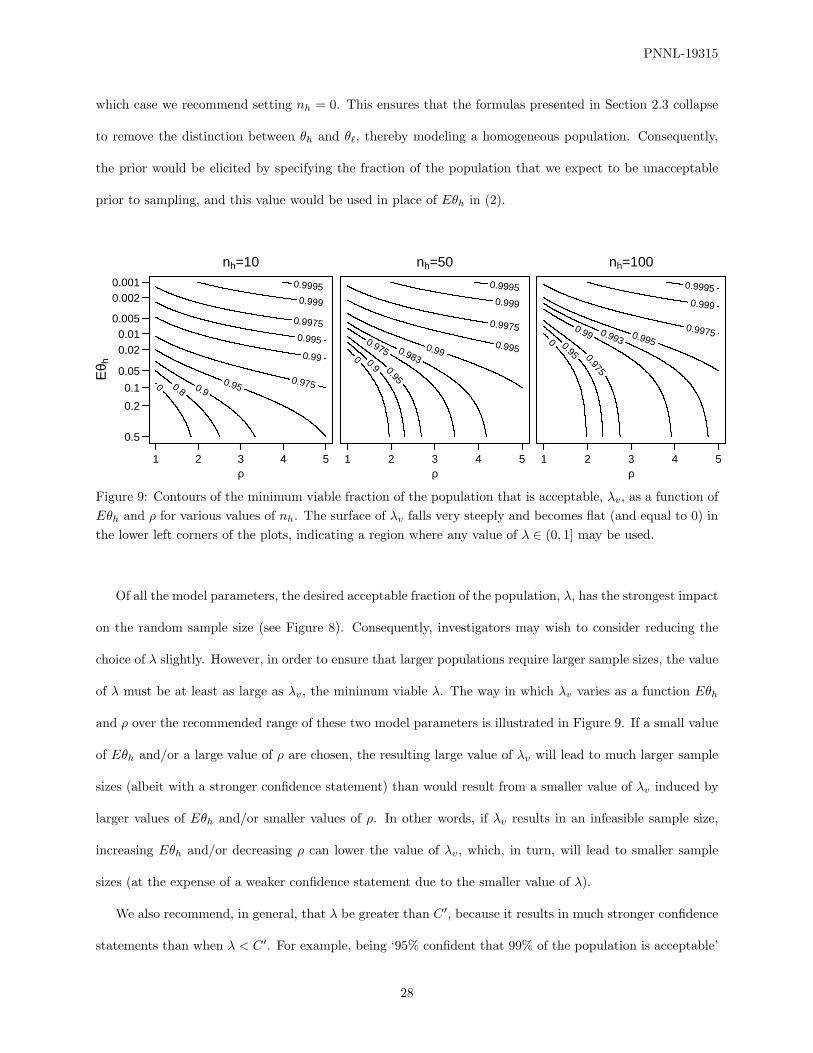
Figure 9: Contours of the minimum viable fraction of the population that is acceptable, λv, as a function ofEθh and ρ for various values of nh. The surface of λv falls very steeply and becomes flat (and equal to 0) inthe lower left corners of the plots, indicating a region where any value of λ ∈ (0, 1] may be used.
Of all the model parameters, the desired acceptable fraction of the population, λ, has the strongest impact
on the random sample size (see Figure 8). Consequently, investigators may wish to consider reducing the
choice of λ slightly. However, in order to ensure that larger populations require larger sample sizes, the value
of λ must be at least as large as λv, the minimum viable λ. The way in which λv varies as a function Eθh
and ρ over the recommended range of these two model parameters is illustrated in Figure 9. If a small value
of Eθh and/or a large value of ρ are chosen, the resulting large value of λv will lead to much larger sample
sizes (albeit with a stronger confidence statement) than would result from a smaller value of λv induced by
larger values of Eθh and/or smaller values of ρ. In other words, if λv results in an infeasible sample size,
increasing Eθh and/or decreasing ρ can lower the value of λv, which, in turn, will lead to smaller sample
sizes (at the expense of a weaker confidence statement due to the smaller value of λ).
We also recommend, in general, that λ be greater than C ′, because it results in much stronger confidence
statements than when λ < C ′. For example, being ‘95% confident that 99% of the population is acceptable’
28
PNNL-19315
is a much stronger statement (and consequently, will require more samples) than being ‘99% confident that
95% of the population is acceptable.’
C’ = 0.95, nh = 10, λ = 0.9935
ρ
200
300
350
400
415 425
430
1.0 1.5 2.0 2.5 3.0
0.5
0.3
0.2
0.1
0.05
0.030.02
0.01
Eθ h
C’ = 0.95, nh = 50, λ = 0.9943
ρ
150
250 300
350 375
400
420 440
1.0 1.5 2.0 2.5 3.0
C’ = 0.95, nh = 100, λ = 0.995
ρ
100 200
250
300 350 400
450
1.0 1.5 2.0 2.5 3.0
C’ = 0.99, nh = 10, λ = 0.9935
ρ
400
500 550
600 625
650 640
660
1.0 1.5 2.0 2.5 3.0
0.5
0.3
0.2
0.1
0.05
0.030.02
0.01
Eθ h
C’ = 0.99, nh = 50, λ = 0.9943
ρ
400 500
550 600
625
650 675
700
1.0 1.5 2.0 2.5 3.0
C’ = 0.99, nh = 100, λ = 0.995
ρ
400 500 550
600 650
700 750
1.0 1.5 2.0 2.5 3.0
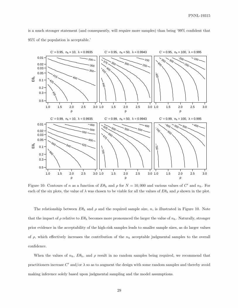
Figure 10: Contours of n as a function of Eθh and ρ for N = 10, 000 and various values of C ′ and nh. Foreach of the six plots, the value of λ was chosen to be viable for all the values of Eθh and ρ shown in the plot.
The relationship between Eθh and ρ and the required sample size, n, is illustrated in Figure 10. Note
that the impact of ρ relative to Eθh becomes more pronounced the larger the value of nh. Naturally, stronger
prior evidence in the acceptability of the high-risk samples leads to smaller sample sizes, as do larger values
of ρ, which effectively increases the contribution of the nh acceptable judgmental samples to the overall
confidence.
When the values of nh, Eθh, and ρ result in no random samples being required, we recommend that
practitioners increase C ′ and/or λ so as to augment the design with some random samples and thereby avoid
making inference solely based upon judgmental sampling and the model assumptions.
29
PNNL-19315
4.4 Software implementation of the CJR method
The CJR methodology has been implemented in Visual Sample Plan (VSP), a freely-available software
tool for the design and analysis of environmental sampling plans (VSP Development Team, 2010). VSP
calculates the Bayesian confidence using (14) and sample sizes using (21), (22), or (23). It also calculates λv
and requires that the user’s choice of λ be at least as large as λv. The CJR method is presented in VSP in
two different modules, one in the context of environmental sampling and the other in the context of discrete
item sampling.
The algorithms for the implementation of the CJR method in VSP were extensively validated by compar-
ing VSP calculations to those produced by routines that were separately coded in the statistical language R
(R Development Core Team, 2010). In a manner similar to the study discussed in Section 3.3, over 163,000
cases were generated so as to span (as much as possible) the subset of P that might be encountered in prac-
tical use. The value of λv and the corresponding random sample size, n, were calculated for each case. The
R and VSP calculations of λv we carried out to 5 decimal places of accuracy and the resulting values were
found to be equivalent in all cases. The random sample sizes (rounded up to the nearest integer) computed
by R and VSP were equivalent in all but a single case, where machine error resulted in a difference of 1
sample.
4.5 Ideas for further research
There are several opportunities for additional research. One of the fundamental premises of the CJR method
is that the high and low-risk groups can be distinguished perfectly before sampling. As this distinction is
likely to be made using professional judgment, it is incumbent to consider what happens when the judgment
is partially, or even completely, wrong. There are a number of ways in which judgmental samples could be
incorrectly chosen—this is briefly discussed and illustrated in Sego (2007, Figure 8). The sensitivity of the
CJR method to misspecification of the high and low-risk groups is the subject of ongoing research.
It would also be advantageous to generalize the CJR method to accommodate more than two risk-based
sub-populations, especially in the context of indoor environmental sampling. Allowing for more than two
groups would make it possible to account for different levels of risk induced by the various factors that
30
PNNL-19315
influence the likelihood of detecting a contaminant at a particular location. These factors may include the
spatial distribution of a contaminant, the persistence and interaction of the contaminant on a particular
surface material, the impact of decontamination, and the sensitivity of the sampling methodology itself.
Investigation of the optimal allocation of samples among the high and low-risk groups (or among multiple
groups) is another area of inquiry. MacQueen (2007) determined that the allocation of samples depends on
the certainty with which items in the population can be classified into the correct risk group. If the risk
groups can be determined with perfect certainty, allocating samples to the highest risk group (until it is
completely sampled), then to the next highest group, and so on, is optimal, in the sense that it will require
the fewest samples to achieve the desired confidence level. However, if the risk groups cannot be determined
with certainty, other types of sample allocation among the groups would be preferable.
The CJR method could also be adapted to account for the probability of false negative measurements,
perhaps using the approach discussed by Axelrod (2005). It would also be desirable to accommodate envi-
ronmental samples obtained via different sampling methodologies (Emanuel et al., 2008, Ch. 5) in the same
decision area. For example, wipe, swab, and vacuum samples each have sampling footprints of different sizes
and different limits of detection.
5 Conclusion
We present a Bayesian model for acceptance sampling where the population consists of two groups, each with
different levels of risk of containing unacceptable items. Expert opinion, or judgment, may be required to
distinguish between the high and low-risk groups. The sampling scheme presumes that all the high-risk items
are sampled (judgmentally) and that a random sample is taken from the low-risk items. For this reason, we
call the approach the combined judgmental and random (CJR) method. Inference is made conditional on
all the observed samples being acceptable, in which case we may conclude with a specified probability that
a high percentage of the items in the population are acceptable.
Special consideration must be taken to ensure the CJR method has desirable analytical properties. In
particular, the required sample size should be a non-decreasing function of the population size, which may
not be the case if the prior belief in the acceptability of the population is so strong that it already satisfies
31
PNNL-19315
the intent to demonstrate (through sampling) that a high percentage of the population is acceptable. In
these situations, the desired fraction of acceptable items must be increased until the Bayesian confidence
function is non-increasing, which then ensures that larger populations will require larger sample sizes.
We demonstrated that the Bayesian acceptance sampling approach presented by Wright (1992) and Grieve
(1994), as well as hypergeometric acceptance sampling, are, in a sense, special cases of the CJR method.
We also illustrate how, even with strong prior belief in the acceptability of the population, attempting to
demonstrate that 100% of the population is acceptable results in unrealistically large sample sizes.
While applicable to a broad range of applications, the CJR method was developed to provide a statistical
model for environmental sampling, particularly inside buildings that may have been contaminated with a
biological or chemical agent. Because the CJR methodology is based on the assumption that all units of
the population are independent, any spatial correlation that may exist among the sampling units is ignored.
However, developing an accurate spatial model when all the sampled items are expected to be acceptable
may be difficult or even impossible. The assumption of independence is conservative, because accounting for
spatial correlation could be used to reduce the number of required samples.
Careful consideration must be made in determining the input parameters for the CJR model. We rec-
ommend that the expected rate of unacceptable high-risk items (Eθh) be chosen between 0.001 and 0.5.
Likewise, we recommend that the ratio of the expected probability of an unacceptable judgmental sample to
the expected probability of an unacceptable random sample, ρ, be chosen between 1 and 5. It is important
to choose a fraction of the population that we wish to demonstrate is acceptable, λ, to be at least as great
as a minimum value of λ that will ensure that the required random sample size increases as the population
size increases. This minimum value is easily calculated as discussed in Section 3.2. The CJR methodology
is implemented in Visual Sample Plan (VSP Development Team, 2010) software and is freely available.
Acknowledgments
This work was funded by the Department of Homeland Security and the National Institute for Occupational
Safety and Health (NIOSH). We express our appreciation to Ryan Orr of Pacific Northwest National Labo-
ratory (PNNL) for his helpful review of this manuscript, and to both Ryan Orr and Stephen Walsh (PNNL)
32
PNNL-19315
for helpful conversations regarding some of the technical details. We also express our appreciation to Randall
Smith (NIOSH) and Yan Jin (NIOSH) for their thorough and thoughtful reviews of the manuscript.
References
Abramowitz, M., and Stegun, I. (Eds.). (1972). Handbook of mathematical functions with formulas, graphs,
and mathematical tables. Washington, D.C.: National Bureau of Standards.
Axelrod, M. (2005). Using ancillary information to reduce sample size in discovery sampling and the effects of
measurement error (Tech. Rep. No. UCRL-TR-216206). Livermore, CA: Lawrence Livermore National
Laboratory. Retrieved 24 August 2010, from https://e-reports-ext.llnl.gov/pdf/324013.pdf
Bowen, W. M., and Bennett, C. A. (1988). Statistical methods for nuclear material management (No.
NUREG/CR-4604). Washington, D.C.: U.S. Nuclear Regulatory Commission.
Cressie, N. (1993). Statistics for spatial data (Revised ed.). Hoboken, NJ: John Wiley & Sons, Inc.
Danaher, P. J., and Hardie, B. G. S. (2005). Bacon with your eggs? Applications of a new bivariate
beta-binomial distribution. The American Statistician, 59 , 282-286.
Emanuel, P., Roos, J. W., and Niyogi, K. (Eds.). (2008). Sampling for biological agents in the environment.
Washington, D.C.: ASM Press.
GAO. (2005). Anthrax detection: Agencies need to validate sampling activities in order to increase confidence
in negative results (Tech. Rep. No. GAO-05-251). Washington, D.C.: United States Government
Accountability Office. Retrieved 24 August 2010, from www.gao.gov/new.items/d05251.pdf
Gelman, A., Carlin, J., Stern, H., and Rubin, D. (2004). Bayesian data analysis (2nd ed.). Boca Raton,
FL: Chapman & Hall/CRC.
Graves, T., Hamada, M., Booker, J., Decroix, M., Chilcoat, K., and Bowyer, C. (2007). Estimating a
proportion using stratified data from both convenience and random samples. Technometrics, 49 ,
164-171.
Grieve, A. P. (1994). A further note on sampling to locate rare defectives with strong prior evidence.
Biometrika, 81 , 787-789.
Gupta, A. K., and Wong, C. R. (1985). On three and five parameter bivariate beta distributions. Metrika,
32 , 85-91.
Guy, D. M., Carmichael, D. R., and Whittington, O. R. (1998). Practitioner’s guide to audit sampling.
33
PNNL-19315
Hoboken, NJ: John Wiley & Sons, Inc.
Hoehn, L., and Niven, I. (1985). Averages on the move. Mathematics Magazine, 58 , 151-156.
Jaech, J. L. (1973). Statistical methods in nuclear material control (Tech. Rep. No. TID-26298). Springfield,
VA: NTIS.
Lee, M.-L. T. (1996). Properties and applications of the Sarmanov family of bivariate distributions. Com-
munications in Statistics–Theory and Methods, 25 , 1207-1222.
MacQueen, D. H. (2007). Material-based stratification (Tech. Rep. No. UCRL-TR-231455). Livermore, CA:
Lawrence Livermore National Laboratory. Retrieved 24 August 2010, from https://e-reports-ext
.llnl.gov/pdf/348316.pdf
Magnussen, S. (2002). An algorithm for generating positively correlated beta-distributed random variables
with known marginal distributions and specified correlation. Computational Statistics & Data Analysis,


![Acceptance Sampling[1]](https://static.documents.pub/doc/80x56/54cd28584a7959f64d8b459c/acceptance-sampling1.jpg)
