arX

iv:a

stro

-ph/

0010

268v

2 3

Jan

200

1

Accepted for publication in The Astrophysical Journal, v. 551 (2001)

Monte Carlo Simulations of Thermal-Nonthermal Radiation from a Neutron

Star Magnetospheric Accretion Shell

Markus Bottcher12 and Edison P. Liang2

ABSTRACT

We discuss the space-and-time-dependent Monte Carlo code we have developed to

simulate the relativistic radiation output from compact astrophysical objects, coupled

to a Fokker-Planck code to determine the self-consistent lepton populations. We have

applied this code to model the emission from a magnetized neutron star accretion shell

near the Alfven radius, reprocessing the radiation from the neutron sar surface. We

explore the parameter space defined by the accretion rate, stellar surface field and the

level of wave turbulence in the shell. Our results are relevant to the emission from atoll

sources, soft-X-ray transient X-ray binaries containing weakly magnetized neutron

stars, and to recently suggested models of accretion-powered emission from anomalous

X-ray pulsars.

1. Introduction

The high energy radiation from compact astrophysical objects is emitted by relativistic

or semi-relativistic thermal and nonthermal leptons (electrons and pairs) via synchrotron,

bremsstrahlung, and Compton processes, plus bound-bound and bound-free transitions of high-Z

elements. Since Compton scattering is a dominant radiation mechanism in this regime, the most

efficient and accurate method to model the transport of high energy radiation is the Monte

Carlo (MC) technique. During the past decade we have developed a versatile state-of-the-art

space-and-time-dependent MC code to model the radiative output of compact objects (see e.g.

Liang et al. 2000). Recently we have added the self-consistent evolution of the leptons using a

Fokker-Planck scheme. The lepton evolution is then coupled to the photon transport. Since this

is the first time that we report on results obtained with this code, the first part of the present

paper is devoted to a detailed description of the capabilities of the code (§2) and its verification in

comparison with previous work (§3).

1Chandra Fellow

2Physics and Astronomy Department, Rice University, MS 108, 6100 S. Main Street, Houston, TX 77005-1892,

USA

– 2 –

In the second part of this paper (§4), we apply this coupled MC-FP code to the study of

the reprocessing of blackbody radiation from a magnetized neutron star surface by a magnetized

spherical shell at the Alfven radius. Recent observations of weak-field neutron star binaries, such

as low-luminosity, X-ray bursters (atoll sources, e.g., 4U 1608-522: Zhang et al. 1996, 4U 1705-44:

Barret et al. 1996), bursting soft X-ray transients (e.g., Aql X-1: Harmon et al. 1996), or pulsar

binary systems (e.g., PSR B1259-63: Tavani et al. 1996) indicate that many of them exhibit soft

(photon index ∼> 2) power law tails extending beyond ∼ 100 keV, at least episodically, in addition

to the thermal component at temperatures of ∼ a few keV, which presumably originates from the

stellar surface. The luminosity of this high-energy tail appears to be anti-correlated with the soft

X-ray luminosity (Barret & Vedrenne 1994, Tavani & Liang 1996).

The origin of this high energy tail is unexplained at present. It could be due to thermal

Comptonization by a hot coronal plasma, or it could be due to nonthermal emission. Tavani and

Liang (1996) examined systematically the possible sites of nonthermal emissions and concluded

that the Alfven surface is the most likely candidate since the dissipation of the rotation energy of

the disk is strongest there, due to magnetic reconnection and wave turbulence generation. Here

we first focus on particle acceleration by wave turbulence.

Because of the 1-D nature of our code at this stage, the neutron star is assumed to emit

isotropic blackbody radiation, the reprocessing magnetospheric plasma is idealized as part of

a spherical shell at the Alfven radius, and the magnetic field is taken to be nondirectional, so

that the radiation output is isotropic. Even though this is not a perfect representation of a

quasi-dipolar magnetosphere and accretion flow, we believe that, except for very special viewing

angles, our output spectra should be a reasonable approximation to the angle-averaged output of

the reprocessing by a hybrid thermal/nonthermal magnetosphere. We assume that the leptons

are energized by Coulomb collisions with virial ions and accelerated nonthermally by Alfven and

whistler wave turbulence, and cooled by cyclotron/synchrotron, bremsstrahlung, and inverse

Comptonization of both internal soft photons and blackbody photons from the stellar surface.

The primary focus of the parameter study presented in §4 is the application to weakly

magnetized neutron stars with surface magnetic fields of Bsurf ∼< 1011 G. In particular, we will

show that the anti-correlation of the hardness and luminosity of the hard X-ray emission with

the soft X-ray luminosity is a natural consequence of the energetics of particle acceleration and

cooling near the Alfven radius. We predict that the nonthermal tails in the hard X-ray spectra of

accreting, weakly magnetized neutron stars may extend up to ∼ 1 MeV. A solid detection and the

measurement of the cutoff energy of these high-energy tails by the INTEGRAL mission, scheduled

for launch in 2002, will provide important constraints on accretion-based models for the hard

X-ray emission from accreting neutron stars.

In this context, it is interesting to note that Chatterjee, Hernquist, & Narayan (2000; see also

Mereghetti & Stella 1995, Wang 1997, Chatterjee & Hernquist 2000) have recently proposed a

similar type of accretion-powered emission for anomalous X-ray pulsars (AXPs), as an alternative

– 3 –

to models based on magnetic-field decay (Thompson & Duncan 1996) or residual thermal energy

(Heyl & Hernquist 1997). According to Chatterjee et al. (2000) the X-ray emission from AXPs

(which generally consists of a soft, thermal component with kT ∼ 0.3 – 0.4 keV plus a hard

X-ray tail with photon index Γ ∼ 3 – 4) is powered by accretion of material from the debris of

the supernova which had formed the neutron star, onto a the surface of the neutron star, which

possesses a typical pulsar magnetic field of Bsurf ∼ 1012 G. Therefore, we extend our parameter

study to parameter values relevant to accreting pulsars. However, we point out that in the case of

a magnetic field as high as Bsurf ∼ 1012 G, the assumed shell geometry and the quasi-isotropy of

the emission from the neutron star surface may be a gross over-simplification. However, although

consequently the precise parameter values used in this region of the parameter space should

not be taken at face value, our parameter study might still provide interesting insight into the

dependence of the equilibrium electron and photon spectra on the various input parameters in the

high-magnetic-field case.

2. Physics of photon and lepton evolution

We use the Monte Carlo (MC) technique (Podznyakov, Sobol, & Sunyaev 1983; Canfield,

Howard, & Liang 1987; Liang 1993; Hua, Kazanas, & Titarchuk 1997) to simulate relativistic

photon transport. We include the full (energy-and-angle-dependent) Klein-Nishina cross section

for Comptonization, relativistic bremsstrahlung from lepton-ion and lepton-lepton scattering

(Dermer 1984), and cyclo-synchrotron processes (Brainerd 1984) in magnetic fields. The MC

photon transport is fully space-and-time-dependent. Photons are born with a certain “weight”

(which is basically the total energy in photons within a spatial region or emitted from a photon

source, divided by the number of Monte-Carlo particles) which is diminished by absorption and

escape, until the weight drops below a user-specified limit, at which point the photon is ”killed”.

In the simulations shown later in the paper, we specify this energy weight cutoff as 1/100 of

the initial statistical weight of the photon. The final results are insensitive to the choice of this

energy weight cutoff, as long as it is ≪ 1. Surviving photons are sampled at boundaries to provide

time-and-frequency-dependent spectral output. In addition to self-emitted photons from the

plasma, soft photons can be injected at zone boundaries and inside volume elements. Currently

the code can handle 1-D spherical, cylindrical or slab geometries with an arbitrary number of

spatial zones. However since the photon ray tracing is done with full angle informations, the

generalization to 2-and-3-D transport is straight forward. The maximum number of photon

frequency bins is 128. For more details of this code see Canfield et al. (1987) and Bottcher &

Liang (1998). A typical MC run with a million particles at a Thomson depth of a few takes

10s of minutes on a DEC alpha server. Since the CPU time usage scales as the square of the

Thomson depth ( number of scatterings), Thomson thick runs can be quite time consuming. We

are currently developing a random walk scheme for Wien photons trapped in Thomson thick

zones, which would save large amounts of CPU time without introducing too much error.

– 4 –

The lepton population is computed locally in each spatial zone using the Fokker-Planck

approximation (Dermer, Miller, & Li 1996; Li, Kusunose & Liang 1996a), taking into account

coulomb and Moller scattering, stochastic acceleration by Alfven and whistler wave turbulence,

and radiative cooling (plus pair processes if necessary). In general the lepton population consists

of a low energy thermal population plus a high-energy tail truncated at the highest energies by

radiative cooling. The photon and lepton evolutions are coupled to each other via a quasi-implicit

time scheme in which we use an average of the photon-electron energy exchange rates between

two subsequent time steps to compute the electron cooling rates, in particular due to Compton

scattering. The Fokker-Planck equation governing the electron evolution is solved using a fully

implicit scheme. In contrast to several other codes currently used in the literature (e.g., Stern et

al. 1995; Li et al. 1996a, Malzac & Jourdain 2000), we solve the evolution of the entire electron

population with the FP scheme and do not introduce any artificial separation between thermal and

non-thermal particles. Since the lepton distribution typically evolves much faster than the photon

distribution, each photon cycle contains many lepton cycles. The user, however, can always turn

off the nonthermal lepton acceleration and assume a strict thermal population whose temperature

can be computed self-consistently from energy balance alone.

In oder to calculate the emissivities and opacities for thermal cyclotron, non-thermal

synchrotron, and thermal bremsstrahlung emission (and only for this purpose), the electron

distribution calculated with our Fokker-Planck scheme is decomposed into a thermal population

plus a non-thermal tail. For the thermal bremsstrahlung and non-thermal synchrotron emission

and absorption, the standard expressions from Rybicki & Lightman (1979) are used. For the

thermal cyclotron emission, we add explicitly over the first 5 harmonics, beyond which we use the

asymptotic continuum representation of Mahadevan, Narayan & Yi (1996).

Since in many cases of interest to the current investigation the moderately to strongly

magnetized coronal plasma is optically thick at low frequencies, hν ≪ 1 keV, due to synchrotron-

(self-)absorption, we use the following simplification in order to save CPU time: For any given

frequency hν ∼< 1 keV, we compare the absorption length lνabs to the Compton mean free path,

lνCompt and the radial extent ∆R of the current zone of the Comptonizing region. If

lνabs < 0.1 min{

lνCompt, ∆R}

(1)

any soft photon produced at this frequency has a very small probability of escaping the current

zone or being up-scattered (to a frequency at which the absorption length will be different so that

the above criterion has to be re-evaluated after the scattering event) before being re-absorbed.

Thus, in the frequency ranges where Eq. (1) is fullfilled, the radiation escaping at the boundary

of that zone will be approximately given by the respective section of the thermal blackbody

spectrum. Accordingly, our code neglects the volume emissivities in those frequency ranges and,

instead, produces thermal blackbody photons at the zone boundaries.

During each photon time step, the code keeps track of the energy transferred between photons

– 5 –

and electrons due to Compton scattering and cyclotron/synchrotron and bremsstrahlung emission

and absorption. The respective heating and cooling rates are used to scale the energy loss/gain

coefficients of electrons at a given energy Ee = γ mec2. For the bremsstrahlung energy loss rate, we

use the approximate scaling law (dγ/dt)br ∝ −γ1.1 (Bottcher, Pohl, & Schlickeiser 1999). Coulomb

heating/cooling is included using the energy exchange and dispersion rates given in Dermer &

Liang (1989). We assume that the ions have a pre-specified temperature kTp ∼> 1 MeV, which is

not significantly affected by any changes of the electron temperature. For the energy exchange

due to Møller scattering (elastic electron-electron scattering) we use the electron energy exchange

and dispersion coefficients given in Nayakshin & Melia (1998).

In addition to Coulomb interactions and radiative losses, we also account for stochastic (2nd

order Fermi) acceleration due to Alfven and Whistler waves. For a given background magnetic

field B, the magnitude and spectrum of hydromagnetic plasma wave turbulences are determined by

the parameters δ2 ≡ (∆B/B)2, where ∆B is the amplitude of the magnetic-field fluctuations, and

q, the spectral index of the turbulence spectrum. We will generally use q = 5/3, characteristic of

Kolmogorov turbulence. The electron acceleration and energy dispersion rates are calculated using

the formalism of Schlickeiser (1989). However, we have to take into account that those plasma

waves interacting efficiently with the low-energy, quasi-thermal part of the electron spectrum will

be efficiently damped and absorbed by the process of Landau damping (e.g., Schlickeiser, Fichtner

& Kneller 1996). This leads to a strong truncation of the Kolmogorov wave spectrum above a

critical wave number for which the equivalent absorption depth through the region occupied by

the hot plasma exceeds unity. We take the effect of Landau damping into account by introducing

an effective absorption depth τk at wave number k, and correcting the acceleration rate γ0A of

Schlickeiser (1989) due to the “optically thin” plasma wave spectrum by an absorption term:

γA = γ0A(1− e−τkres )

τkres. (2)

Here τkres = Γkres tA, and Γk is the Landau damping rate at wave number kres at which Alfven

waves are resonating preferentially with electrons of energy γ. tA = ∆R/vA is the Alfven crossing

time of the zone. This modified acceleration term can be renormalized either to correspond to

the pre-specified value of δ2 for electrons resonating with waves in the weakly damped part of the

Alfven wave spectrum (i.e. at high electron energies), or by specifying a heat input rate into the

electron ensemble due to resonant wave/particle interactions.

As an option, our code can account for pair production and annihilation and the corresponding

photon absorption and emission. The pair annihilation rates and annihilation radiation emissivities

are taken from Svensson (1982), and the γγ pair production rate of Bottcher & Schlickeiser

(1997) is used. In addition, simple Compton reflection schemes, using the Green’s functions for

reflection off neutral disk material of White, Lightman & Zdziarski (1988) and Lightman & White

(1988), can be used to simulate a Compton reflection component either off the inner boundary

(corresponding to a quasi-homogeneous slab geometry) or reflecting part of the radiation escaping

– 6 –

at the outer boundary (e.g., corresponding to a cold outer disk).

Assuming local isotropy of the electron distribution, we solve the one-dimensional

Fokker-Planck equation

∂ne(γ, t)

∂t= − ∂

∂γ

[

ne(γ, t)dγ

dt

]

+1

2

∂2

∂γ2[ne(γ, t)D(γ, t)] , (3)

where D is the energy dispersion coefficient. To solve Eq. 3, we use an implicit version of the

discretization scheme proposed by Nayakshin & Melia (1998). We choose a logarithmic spacing in

electron kinetic energy, xi ≡ γi − 1. In the following the subscript i refers to electron energy, while

the superscript n refers to time. We define fni ≡ ne(γi, t

n)/ne The discritization is then given by

fni = fn+1

i +∆t

(

an+1i+1 f

n+1i+1 − an+1

i−1 fn+1i−1

∆xi +∆xi−1

)

−∆t

(

αDn+1i+1 f

n+1i+1 − 2Dn+1

i fn+1i + ρDn+1

i−1 fn+1i−1

α∆xi(∆xi−1 +∆xi)

)

, (4)

where ai = (dγ/dt)(xi), Di = [d(∆γ)2/dt](xi), α = 2/(1 + q), ρ = 2q/(1 + q), with q = xi+1/xi.

The system of equations is supplemented by the boundary conditions specified in Appendix A of

Nayakshin & Melia (1998). The system of equations (4) is in tridiagonal form and can be easily

solved to find the electron distribution at time tn+1. In order to evaluate the energy exchange and

dispersion coefficients an+1i and Dn+1

i the code performs an energy balance calculation to find the

average electron energy in the ensemble after the current time step, which is then used to calculate

the energy exchange and dispersion coefficients due to Møller scattering. All other coefficients

evolve sufficiently slowly (i.e. on time scales much longer than the electron-evolution time scale)

so that the coefficients evaluated under the conditions at the beginning of the current time step

can be used.

The implicit scheme of Eq. 4 is known to approach the equilibrium solution for the electron

distribution exactly, although the temporal evolution calculated this way becomes inaccurate

on short time scales. Since in the problems of interest here, the electron distributions typically

evolve on timescales much shorter than the photon distributions, the electrons always attain a

distribution close to local equilibrium during each photon time step. Hence, the degree of accuracy

provided by the implicit scheme is sufficient for our purposes. As an option, the code can perform

the same simulations using an explicit scheme to solve the Fokker-Planck equation. In all test

cases, both schemes produced virtually identical results, but the implicit scheme executes a factor

of ∼ 10 – 100 faster because of the larger individual Fokker-Planck time steps allowed in this

scheme.

However, we did not find an appropriate method to calculate the coefficients for the pair

production and annihilation rates at time step n + 1. For this reason, we have to correct the

electron and positron distribution functions for pair production and annihilation in an explicit

manner. This becomes obviously inaccurate in the case of strongly pair producing model

– 7 –

situations. Thus, our scheme is a significant improvement over existing schemes only for pair

deficient situations with pair fractions fpair ≡ ne+/np ∼< a few %. For strongly pair dominated

situations, we would have to adjust the individual time steps of our simulations so far that such

simulations would take a prohibitive amount of computing time.

In the present paper, we focus on results for equilibrium situations, for which we let the

code evolve until a stable electron distribution and photon output spectrum is reached. The

convergence of the electron and photon spectra can be greatly accelerated if one starts out with

an appropriate first guess for the equilibrium electron temperature. For this reason, we have

developed an analytical estimate of the equilibrium electron temperature, which is described in

Appendix A. This analytical estimate is implemented in our code and can be used to determine

the appropriate initial conditions for our equilibrium simulations. Detailed tests and applications

of the time-dependent features of the code will be presented in future publications.

3. Tests of the numerical scheme and comparison with Previous Results

For verification of our code, we have first compared the individual energy exchange and

diffusion rates, dγ/dt and D(γ), with those obtained in earlier work. Our numerical energy

exchange and diffusion rates due to Coulomb scattering are in agreement with those of Dermer

& Liang (1998)3. The numerical values of the Møller scattering energy exchange and diffusion

coefficients were found in good agreement with those of Nayakshin & Melia (1998)4.

We have verified that in cases in which radiative cooling and hydromagnetic acceleration

are inefficient, our Fokker-Planck scheme correctly produces a thermal electron distribution in

temperature equilibrium with the protons.

In the analysis of coronal energy and radiation transfer, it is customary to paramatrize

energy input and dissipation rates u [ergs cm−3 s−1] by the dimensionless compactness, l, which in

spherical geometry, is defined by lsph ≡ 4πσT R2 u/(3mec3), where R is the radius of the spherical

volume. In slab geometry, this becomes lslab ≡ σT H2u/(mec3), where H is the thickness of the

slab. In our simulations, we specify the heating mechanisms to be Coulomb heating through the

thermal protons and resonant wave-particle interactions. Thus, leaving the shape of the electron

spectrum general, we calculate the respective energy dissipation rates as

uCoul/A = mec2

∞∫

1

dγ ne(γ)

(

dγ

dt

)

Coul/A, (5)

3note that in their Eq. (A2), the last γ∗ has to be replaced by (γ∗)2

4note that there is a ’-’ sign missing in front of the term ∝ (γ − γ1)2 in their Eq. (35)

– 8 –

where the subscript ’Coul/wp’ stands for Coulomb scattering and wave-particle interaction,

respectively. Obviously, the resulting compactness will depend not only on the energy density in

protons and magnetic turbulence, but also on the current electron distribution (i.e. temperature,

if the distribution is predominantly thermal), and can thus not be specified a priori as a free

parameter. For comparison with previous work, we need to find appropriate values of the

ion temperature and the wave turbulence amplitude in order to reproduce the dissipation

compactness quoted in those papers. We define the temperature corresponding to the electron

spectrum resulting from our simulations by requiring that the average electron Lorentz factor,

〈γ〉 = (1/ne)∫

dγ γ ne(γ), be equal to the average Lorentz factor of a thermal electron population

of the respective temperature,

〈γ〉th =K3

(

1Θe

)

K2

(

1Θe

) −Θe. (6)

To test our energy balance calculations, we have performed a series of simulations to reproduce

the results of the slab corona model of Dove et al. (1997), in particular the inset of their Fig.

2, with which we find good agreement. For those simulations, we specified ion temperatures of

80 MeV ∼< kTi ∼< 250 MeV, a magnetic field in equipartition with the ion population, and a

negligibly low level of Alfven wave turbulence to reproduce various values of the local heating

compactness lc. As mentioned earlier, our code is rather inefficient in simulating strongly

pair-producing, high-lc situations because of the explicit scheme to solve for pair balance. For this

reason, we restrict the applications of the code in its present version to model situations with pair

fractions ∼< a few %.

Li et al. (1996a, b) have developed a code solving simultaneously the Fokker-Planck equations

for both the electron and the photon distribtions in a homogeneous medium, including Coulomb

interactions, thermal bremsstrahlung, Compton scattering, resonant wave-particle interactions,

and pair production and annihilation. There are two major differences between their approach

and ours: (1) We use a Monte-Carlo method to solve the photon transport, and (2) we solve

the Fokker-Planck equation for the entire electron spectrum, while Li et al. (1996a, b) split the

electron distribution up into a thermal “bath” plus a non-thermal tail, assuming a priori that

electrons of energies γ < γthr = 1+4Θe attain a thermal distribution, and that acceleration due to

wave/particle interactions affects only particles beyond γthr. The latter simplification is justified

by the argument that at low electron energies the thermalization time scale is much shorter than

any other relevant time scale, and that long-wavelength plasma waves, with which low-energy

electrons resonate preferentially, are strongly damped and in energy elequilibrium with the thermal

pool of electrons. In our simulations, both effects are taken into account self-consistently without

making the a-priori assumption of the existence or development of a non-thermal population.

Li et al. (1996b) present two model calculations to explain hard tails observed in the

hard X-ray / soft γ-ray spectra of Cyg X-1 and GRO J0422+32. A spherical region of radius

– 9 –

R = 1.2× 108 cm is assumed. For the case of Cyg X-1, they specify a total heating compactness of

l = 4.5, and a non-thermal heat input into suprathermal particles (γ > γthr) of lst/l = 0.15, wich a

turbulence amplitude of δ2 = 0.059. A soft blackbody radiation component at kTs = 0.1 keV from

the outer boundary of the sphere is assumed to provide a soft radiation compactness of ls/l = 0.07.

The seed Thomson depth of the region is τp = 0.7. In their simulations, Li et al. (1996b) find a

significant suprathermal tail in the resulting electron distribution, which leads to an excess hard

X-ray / soft γ-ray emission, consistent with the observed one. The temperature of the thermal

part of their electron ensemble is found at kTe = 139 keV, and the equilibrium pair fraction is

fpair ≈ 1.8 %. For the case of GRO J0422+32 they specify l = 0, lst/l = 0.06, and ls/l = 0.08.

This resulted in a weaker nonthermal electron tail, an equilibrium temperature of kTe = 133 keV,

a wave amplitude of δ2 = 0.065, and a pair fraction of fpair ≈ 3 %.

For comparison with our code, we have run simulations with the same total compactness l,

soft compactness ls, soft blackbody temperature kTBB, radius R, seed Thomson depth τp, and

the same values of the plasma wave amplitude normalization δ2. A difficulty in comparing the

two codes is that in Li et al. (1996a, b) the ion temperature and magnetic field are not specified

explicitly. In our comparative simulations we assume a magnetic field in equipartition with the

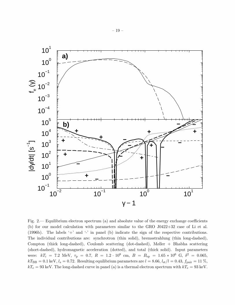
ion energy density. The results of our simulations are illustrated in Figs. 1 and 2. Our results

are qualitatively similar to those of Li et al. (1996a, b). However, we find somewhat lower

equilibrium temperatures and stronger nonthermal electron tails as well as stronger suprathermal

acceleration compactnesses lst. The lower temperatures may be attributed to a rather prominent

cyclotron/synchrotron cooling (comparable to Compton cooling) in our simulations (see Figs. 1b

and 2b). This, in combination with the larger lst values, seems to indicate that in our simulations

we have used higher magnetic field values than Li et al. (1996a, b). However, even abandoning

the equipartition assumption, we could not find self-consistent parameter values resulting in the

same combination of input parameters used by Li et al. (1996a, b). Given this descrepancy in

the way of input parameter specification, the qualitative agreement between the results of the two

codes, using very different numerical methods, is encouraging.

4. Models of accretion onto a magnetized neutron star

While in the first part of this paper we were describing the general features and the verification

of our MC/FP code, we are now applying this code to model the electron dynamics and photon

transport arising from models of accretion onto a magnetized neutron star. In both weakly

magnetized neutron stars (atoll sources and soft X-ray transient neutron star binary systems)

with Bsurf ∼< 1011 G and X-ray pulsars (including, possibly, anomalous X-ray pulsars) with

Bsurf ∼ 1012 G, energy dissipation will be most efficient at the Alfven radius, where the optically

thick, geometrically thin outer accretion disk is disrupted and the dynamics of the accretion flow

becomes dominated by the magnetic field. We idealize this region of efficient energy dissipation

at the Alfven radius of disk accretion onto a magnetized neutron star as part of a spherical shell

– 10 –

whose distance r0, magnetic field, and column thickness are fixed by the accretion rate (Ghosh &

Lamb 1979a,b,1990). The distance r0 is given by

r0 = 2× 108 f µ4/730 l

−2/7∗ M

−1/7∗ R

−2/76 cm (7)

where µ30 = (neutron star magnetic moment)/(1030 Gcm3), l∗ = L/LEdd, M∗ = MNS/M⊙, and

R6 = RNS/(106 cm). For the current simulations, for definiteness, we fix the Ghosh-Lamb fudge

parameter f = 0.3, and set M∗ = R6 = 1. Hence, the dipole magnetic field at the Alfven radius is

B0 = 4.2× 106 l6/7∗ µ

−5/730 M

3/7∗ R

6/76 f−3

0.3 G, (8)

where f0.3 = f/0.3. The virial ion temperature at r0 is

kTi =2

3

GM mH

r0≈ 9.3

(

r0107 cm

)−1

M∗ MeV. (9)

The column density of the shell can be estimated using the poloidal accretion rate

M ∼ 4πr0 ∆r0 ni vpmH , where we assume that the poloidal velocity vp ∼ vff/2 with vffbeing the free-fall velocity. Hence, the radial Thomson depth of the shell is approximately:

τT = ∆r0 ni σT ∼ M σT2πr0 vff mH

≈ 0.97 l8/7∗ µ

−2/730 M

4/7∗ R

1/76 f

−1/20.3 . (10)

The neutron star (taken to be a 10 km spherical surface) is assumed to emit a blackbody luminosity

at the temperature kTBB = 1.78 l1/4∗ keV. In addition the level of wave turbulence is specified by

the dimensionless amplitude δ2 = (∆B/B)2 and the spectral index q. The minimum wavevector

kmin is set to 2π/(∆r0), where ∆r0 ∼ 0.1r0 is the shell thickness (Ghosh & Lamb 1979a,b, 1990).

Due to spherical symmetry of our simulations the magntic field is assumed to be nondirectional in

the shell and the synchrotron emissivities and absorption coefficients are angle-averaged.

We have explored the parameter space by varying the accretion rate — corresponding to a

variation of the parameter l∗ —, the magnetic field — corresponding to a variation of µ30 —, and

the amplitude of wave turbulence, δ2. q is set = 5/3 in all runs presented in this paper.

In Fig. 3, we demonstrate the effect of a varying accretion rate in the case of no turbulence,

δ2 = 0, and for a fixed magnetic moment of the neutron star, µ30 = 1, corresponding to a strong

surface field of Bsurf ∼ 1012 G. As the accretion rate decreases, the Alfven radius moves outward,

implying a lower magnetic field at the Alfven radius, and a lower ion temperature and Thomson

depth of the active shell. At the same time, however, Compton cooling becomes less efficient

due to the reduced soft photon luminosity of the neutron star surface and due to the larger

distance of the active region from the surface. This reduction of the soft photon compactness

leads to an increasing equilibrium electron temperature in the accretion shell. Consequently, as

the accretion rate decreases, the photon spectra change in the following way: For l∗ = 1, the

– 11 –

hard X-ray spectrum smoothly connects to the peak of the thermal blackbody bump from the

neutron star surface, and shows a quasi-exponential cutoff at high energies. For lower l∗, the

spectrum turns into a typical low-hard state spectrum of X-ray binaries with the thermal bump

clearly distinguished from a hard power-law + exponential cutoff at high energies. The hard X-ray

power-law becomes harder with decreasing l∗. Fig. 4 shows the same sequence of decreasing l∗for µ30 = 10−3, corresponding to Bsurf ∼ 109 G. At high accretion rates, a strong reduction of

the equilibrium electron temperature with respect to the strong-field case results, leading to a

softening of the photon spectrum with decreasing µ30. This is due to the increasing magnetic field

at the Alfven radius as the neutron star magnetic moment decreases (because the Alfven radius

decreases, overcompensating for the decreasing magnetic moment, see Eq. 8), resulting in a lower

electron temperature caused due to increasing cyclotron/synchrotron cooling. For low accretion

rates (l∗ ∼< a few %) the electron and photon spectra for the strong-field case and the low-field

case are virtually indistinguishable from each other.

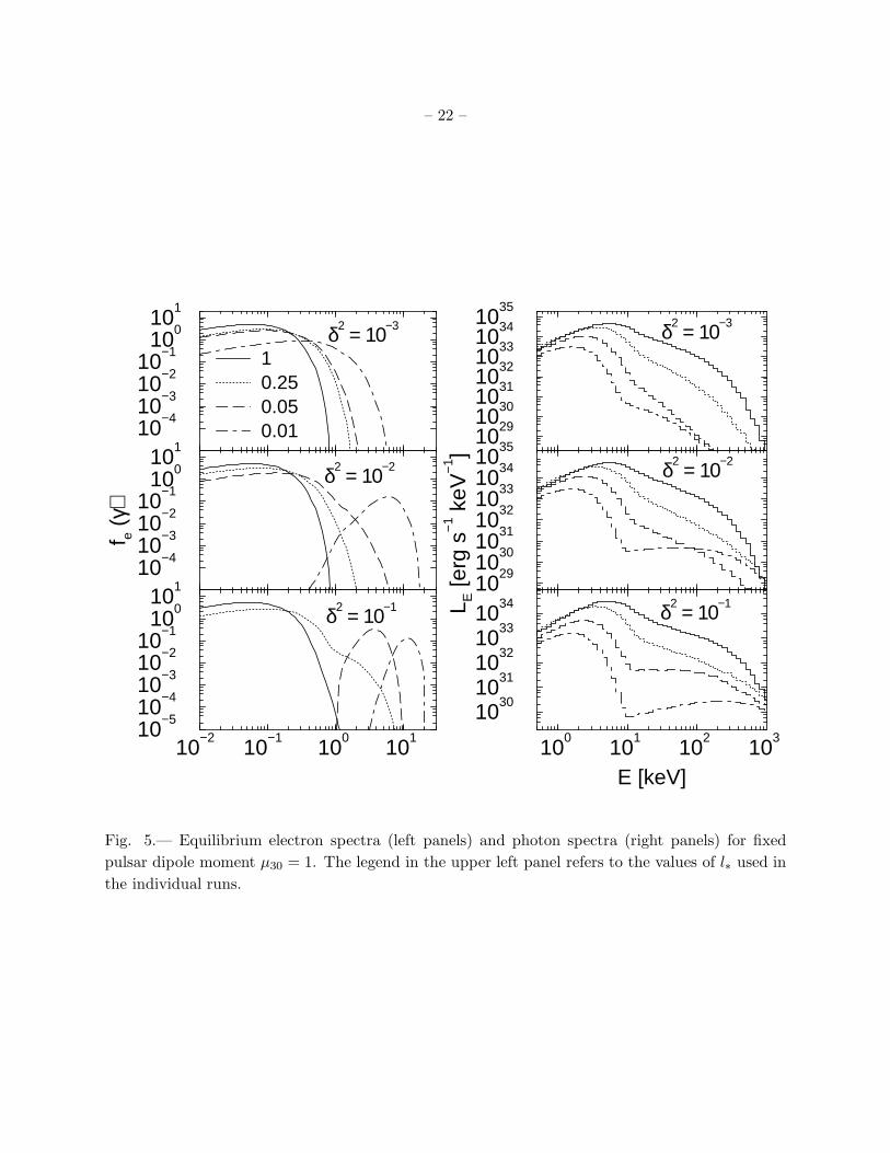
Figs. 5 and 6 illustrate the effects of a varying accretion rate and turbulence level on

the electron and photon spectra. An increasing turbulence level, obviously, leads to a more

pronounced nonthermal tail or bump in the electron spectrum. At the same time, as a result of

increased Compton cooling on synchrotron photons produced by the nonthermal electrons, the

temperature of the quasi-thermal portion of the electron spectrum decreases as the turbulence level

is increasing. Consequently, the photon spectrum at soft to medium-energy X-rays becomes softer

with increasing δ2, while at hard X-ray and γ-ray energies an increasingly hard tail develops. As

in the case without turbulence, a decreasing accretion rate leads to a higher electron temperature

and the transition from a smoothly connected thermal blackbody + thermal Comptonization

power-law spectrum to a typical low/hard state X-ray binary spectrum.

Fig. 7 demonstrates the moderate dependence, in particular of the resulting photon spectra,

on the magnetic moment of the neutron star for an intermediate value of the accretion rate,

l∗ = 0.25. Nonthermal tails in the electron spectra become more pronounced with increasing

neutron star magnetic moment. For the weak-field case with µ30 = 10−3, we find that the

high-energy end of the electron spectra are always truncated with respect to a thermal distribution

due to strong Compton losses, rather than developing a non-thermal tail.

At very low accretion rates, resulting in very low proton and electron densities in the accretion

shell, we find that even at low turbulence level the heating due to stochastic acceleration strongly

dominates over Coulomb heating. Consequently, the resulting electron spectrum becomes strongly

non-thermal. We need to point out that in those cases, our treatment is no longer self-consistent

since in our code the attenuation of Alfven waves is calculated under the assumption that it is

dominated by Landau damping in a thermal background plasma.

The results illustrated in Figs. 4 and 6 are in excellent agreement with the general trend

(Barret & Vedrenne 1994, Tavani & Liang 1996) that hard tails in LMXBs and soft X-ray

transients containing weakly magnetized neutron stars are only observed during episodes of low

– 12 –

soft-X-ray luminosity. While at large soft-X-ray luminosity, the X-ray emission out to ∼> 20 keV

is dominated by the thermal component from the neutron star surface and the hard tail is very

soft with a low cut-off energy at Ec ∼ 100 keV, in lower-luminosity states the hard X-ray tail

becomes very pronounced with photon indices Γ ∼ 2 – 3 and extends out to Ec ∼< 1 MeV.

Dedicated deep observations by the upcoming INTEGRAL mission should be able to detect this

hard X-ray emission from neutron-star-binary soft X-ray transients and atoll sources in both high

and low soft-X-ray states and thus provide a critical test of this type of accretion model for weakly

magnetized neutron stars.

Interestingly, a similar anti-correlation of the hard X-ray spectral hardness with the soft

X-ray luminosity seems to exist for high surface magnetic fields (see Figs. 3 and 5) only in the

case of very low accretion rates (l∗ ∼ 0.01) and rather high magnetic turbulence levels (δ2 ∼> 0.01).

The hard X-ray spectral indices resulting from our simulations are in excellent agreement with the

values of Γ ∼ 3 – 4 generally observed in anomalous X-ray pulsars. This may provide additional

support for accretion-powered emission models for AXPs. Our simulations predict cutoff energies

of Ec ∼ 100 – 500 keV.

5. Summary and Conclusions

We have reported on the development of a new, time-dependent code for radiation

transport and particle dynamics. The radiation transport, accounting for Compton scattering,

bremsstrahlung emission and absorption, cyclotron and synchrotron emission and absorption,

and pair processes, is done using a Monte-Carlo method, while the electron dynamics, including

radiative cooling, Compton heating/cooling, and stochastic acceleration by resonant interaction

with Alfven/whistler wave turbulence, are calculated using an implicit Fokker-Planck scheme,

coupled to the Monte-Carlo radiation transfer code.

In the second part of this paper, we have applied our code to the static situation of a shell at

the Alfven radius of a magnetized neutron star. This situation is representative for accretion onto

weakly magnetized neutron stars (bursting atoll sources or soft X-ray transients containing wekaly

magnetized neutron stars) as well as to recently suggested models of accretion-powered emission

from anomalous X-ray pulsars.

The main results of our parameter study are:

(1) The lepton thermal temperature increases, and the hard X-ray photon spectrum becomes

harder as the accretion rate is decreasing. At the same time, the normalization of the hard X-ray

power-law, relative to the thermal blackbody from the neutron star surface, becomes smaller.

(2) The nonthermal tails in the electron and photon spectra become more dominant and

harder as the turbulence level is increasing. At the same time, the quasi-thermal electron

temperature decreases, leading to a softer hard-X-ray spectrum.

– 13 –

(3) For low accretion rates (∼< a few %), the photon spectra are only very weakly dependent

on the magnetic moment of the neutron star. For higher accretion rates, an increasing neutron

star magnetic moment leads to a moderate hardening of the hard X-ray spectrum.

Our results are in good agreement with the non-detection of hard X-ray tails during soft

X-ray high states of systems containing weakly magnetized neutron stars. However, we predict

that a hard X-ray excess beyond ∼ 20 keV should exist even in the high/outburst state. This

excess should have a cutoff energy of Ec ∼ 100 – 200 keV. In the low/quiescent state, the predicted

spectral indices of Γ ∼ 2 – 3 are in excellent agreement witht he observed hard X-ray excesses

observed from sources believed to contain weakly magnetized neutron stars. We predict that these

spectra should extend out to Ec ∼< 1 MeV.

In the strong-field case, representative of a recently suggested model for anomalous X-ray

pulsars, we expect a strong correlation between the hard X-ray spectral hardness and the soft

X-ray luminosity only in the case of very low accretion rates and high magnetic turbulence level.

The predicted hard X-ray spectral indices are generally in very good agreement with the observed

values of Γ ∼ 3 – 4. Cutoff energies of Ec ∼ 100 – 500 keV are predicted.

Dedicated, deep observations by the upcoming INTEGRAL mission should be able to

establish the existence of the hard power-law tails predicted in the models discussed here, and to

constrain the high-energy cutoff of these tails. These measurements will be essential ingredients

for a more detailed modeling of the physical conditions governing the accretion onto magnetized

neutron stars.

The work of MB is supported by NASA through Chandra Postdoctoral Fellowship Award No.

9-10007, issued by the Chandra X-ray Center, which is operated by the Smithsonian Astrophysical

Observatory for and on behalf of NASA under contract NAS 8-39073. This work was partially

supported by NASA grant NAG5-4055. We wish to thank the referee for very helpful comments,

and D. Marsden for pointing out the relevance of our work to anomalous X-ray pulsars.

A. Estimate of equilibrium temperature

The code outlined above can be used for equilibrium situations by simply letting it evolve

until both the photon and electron distributions have relaxed to a steady state. In order to provide

a consistency test of our numerical methods, we compute a quasi-analytical estimate for the

expected equilibrium electron temperature. In our equilibrium simulations, we use this estimated

equilibrium temperature as initial condition in order to accelerate the convergence.

Assuming that the electron distribution is roughly thermal, we may estimate the heating and

cooling rates due to the various processes as follows. Let

– 14 –

W =1

ne

dE

dV=

3

2k Te (A1)

be the average energy per electrons. We approximate the cyclotron emissivity by the high-frequency

continuum limit given in Mahadevan et al. (1996):

jν(Θe) =21/6

35/6π3/2e2 ne ν

cK2

(

1Θe

)

v1/6exp

[

−(

9v

2

)1/3]

, (A2)

where Θe = kTe/(mec2), v ≡ ν/(νcΘ

2e), and νc = eB/(2πmec).

Denoting by ∆R the thickness of the emitting shell or slab, the synchrotron-self-absorption

frequency is then determined by solving for

1 = ∆RκSSA = ∆Rjν(Θe)

Bν(Θe). (A3)

The cyclotron/synchrotron cooling rate may then be estimated as

(

dW

dt

)

sy

=1

ne V

Asurface

νSSA∫

0

dν Bν(Θe) + V

∞∫

νSSA

dν jν(Θe)

, (A4)

where V and Asurface are the volume and the surface area of the emitting shell or slab.

Assuming that the photon field inside the emitting volume is dominated by low-energy

photons with ǫ ≪ Θe, where ǫ = hν/(mec2), the Compton cooling rate may be approximated as

(

dW

dt

)

IC

= −4c σT uph Θe

K3

(

1Θe

)

K2

(

1Θe

) . (A5)

The photon energy density uph is calculated iteratively from the contributions of the various soft

photon fields, and repeated Compton scatterings: Assume that the soft photon energy density

us = usy +ubr +uext (sycnhrotron + bremsstrahlung + external radiation field) is centered around

a soft photon energy ǫs, and that τT ∼< 1. The average energy change of a photon with mean

photon energy ǫk (Compton scattered k times) changes on average by a factor ∆ǫk = ǫk (4Θ − ǫk)

in the course of the k + 1. scattering. Then, the total internal photon energy density is

uph = us

(

1 +∞∑

n=1

τnT

n−1∏

k=0

[4Θe − ǫk]

)

, (A6)

where ǫ0 = ǫs and ǫk+1 = ǫk (1 + 4Θe − ǫk).

– 15 –

In the cases we are interested in, the bremsstrahlung photon input will be negligible compared

to cyclotron/synchrotron and the external soft photon fields. Thus, we assume us = uext + usywith

uext =Fext

c(A7)

and

usy =1

c

νSSA∫

0

dν Bν(Θe) +∆R

c

∞∫

νSSA

dν jν(Θe). (A8)

The photon energy ǫs is ǫext if uext > usy, or max{ǫSSA, ǫ0} else, where ǫ0 = (hνc/mec2).

The bremsstrahlung cooling rate is

(

dW

dt

)

br

= −{

1283√πα r2e mec

3 ne

√Θe for Θe ≪ 1

96α r2e mec3 neΘe (ln[2Θe] + 0.673) for Θe ∼> 1

(A9)

(Haug 1985) where α = 1/137 is the fine structure constant and re is the classical electron radius.

The heating rate due to Alfven wave turbulence is either specified as a fixed parameter, or

can be evaluated using the acceleration rates according to Eq. (2) as

(

dW

dt

)

A

= mec2

∞∫

1

dγ γA fe(γ). (A10)

Finally, the Coulomb heating / cooling rate is

(

dW

dt

)

Coul

=3

2

me

mpln Λnp c σT (kTp − kTe)h(Θe,Θp), (A11)

where

h(Θe,Θp) =

√Θe

(Θe +Θp)3/22 (Θe +Θp)

2 + 2 (Θe +Θp) + 1

K2

(

1Θe

) exp

(

− 1

Θe

)

(A12)

(Dermer 1986), ln Λ is the Coulomb logarithm, np is the number density of ions, and

Θp = kTp/(mpc2), .

The total heating/cooling rate consists the sum of all elementary processes,

(

dW

dt

)

total

=

(

dW

dt

)

Coul

+

(

dW

dt

)

A

+

(

dW

dt

)

sy

+

(

dW

dt

)

IC

+

(

dW

dt

)

br

, (A13)

and we are iteratively solving for the equilibrium solution(s) with(

dWdt

)

total= 0.

– 16 –

REFERENCES

Barret, D., & Vedrenne, G., 1994, ApJS, 92, 505

Barret, D., et al., 1996, A&AS, 120, 121

Bottcher, M., & Liang, E. P., 1998, ApJ, 506, 281

Bottcher, M., Pohl, M., & Schlickeiser, R., 1999, Astrop. Phys., 10, 47

Bottcher, M., & Schlickeiser, R., 1997, A&A, 325, 866

Brainerd, J., 1984, Ph.D. Thesis, Rice University

Canfield, E., Howard, W. M., & Liang, E. P., 1987, ApJ, 323, 565

Chatterjee, P., Hernquist, L., & Narayan, R., 2000, ApJ, 534, 373

Chatterjee, P., & Hernquist, L., 2000, ApJ, 543, 368

Dermer, C. D., 1984, ApJ, 280, 328

Dermer, C. D., 1986, ApJ, 307, 47

Dermer, C. D., & Liang, E. P., 1989, ApJ, 339, 512

Dermer, C. D., Miller, J. A., & Li, H., 1996, ApJ, 456, 106

Dove, J. B., Wilms, J., & Begelman, M. C., 1997, ApJ, 487, 747

Ghosh, P., & Lamb, F., 1979a, ApJ, 232, 259

Ghosh, P., & Lamb, F., 1979b, ApJ, 234, 296

Ghosh, P., & Lamb, F., 1990, in “Neutron Stars”, ed. J. Ventura (Kluwer Acad., Amsterdam)

Harmon, B. A., Wilson, C. A., Tavani, M., Zhang, S. N., Rubin, B. C., Paciesas, W. S., Ford, E.

C., & Kaaret, P., 1996, A&AS, 120, 197

Hua, X.-M., Kazanas, D., & Titarchuk, L., 1997, ApJ, 428, L57

Haug, E., 1985, A&A, 148, 386

Heyl, J. S., & Hernquist, L., 1997, ApJ, 489, L67

Li, H., Kusunose, M., & Liang, E. P., 1996a, ApJ, 460, L29

Li, H., Kusunose, M., & Liang, E. P., 1996b, A&AS, 120, 167

Liang, E. P., 1993, AIP Conf. Proc. 280, Compton Gamma-Ray Observatory, ed. M. Friedlander,

N. Gehrels, & D. J. Macomb (New York: AIP), 418

– 17 –

Liang, E. P, Bottcher, M., Lin, D., & Smith, I. A., AIP Conf. Proc. 510, 245, ed. McConnell, M.

L., & Ryan, J. M. (AIP, New York)

Lightman, A. P., & White, T. R., 1988, ApJ, 335, 57

Mahadevan, R., Narayan, R., & Yi, I., 1996, ApJ, 465, 327

Malzac, J., & Jourdain, E., 2000, A&A, in press

Mereghetti, S., & Stella, L., 1995, ApJ, 442, L17

Nayakshin, S., & Melia, F., 1998, ApJS, 114, 269

Pozdnyakov, L. A., Sobol, I. M., & Sunyaev, R. A., 1983, Sovjet Scient. Rev. Section E,

Astrophysics and Space Physics Rev., 2, 189

Rybicki, G. B., & Lightman, A. P., 1979, “Radiative Processes in Astrophysics”, John Wiley &

Sons, New York

Schlickeiser, R., 1989, ApJ, 336, 243

Schlickeiser, R., Fichtner, H., & Kneller, M., 1996, JGR, 102, 4725

Stern, B. E., Begelman, M. C., Sikora, M., & Svensson, R., 1995, MNRAS, 272, 291

Svensson, R., 1982, ApJ, 258, 321

Tavani, M., et al., 1996, A&AS, 120, 221

Tavani, M., & Liang, E. P., 1996, A&AS, 120, 133

Thompson, C., & Duncan, R. C., 1996, ApJ, 473, 322

Wang, J. C. L., 1997, ApJ, 486, L119

White, T. R., Lightman, A. P., & Zdziarski, A. A., 1988, ApJ, 331, 939

Zhang, S. N., et al., 1996, A&AS, 120, 279

This preprint was prepared with the AAS LATEX macros v4.0.

– 18 –

10−2

10−1

100

101

γ − 1

10−1

100

101

102

103

104

105

|dγ/

dt| [

s−1 ]

10−4

10−3

10−2

10−1

100

101

f e (γ

)

−

−

−−

+−

+−

++

+

+−

+

+

−

a)

b)

Fig. 1.— Equilibrium electron spectrum (a) and absolute value of the energy exchange coefficients

(b) for our model calculation with parameters similar to the Cyg X-1 case of Li et al. (1996b).

The labels ‘+’ and ‘-’ in panel (b) indicate the sign of the respective contributions. The

individual contributions are: synchrotron (thin solid), bremsstrahlung (thin long-dashed), Compton

(thick long-dashed), Coulomb scattering (dot-dashed), Møller + Bhabha scattering (short-dashed),

hydromagnetic acceleration (dotted), and total (thick solid). Input parameters were: kTi =

3.5 MeV, τp = 0.7, R = 1.2 ·108 cm, B = Bep = 1.1∗106 G, δ2 = 0.059, kTBB = 0.1 keV, ls = 0.315.

Resulting equilibrium parameters are l = 4.43, lst/l = 0.46, fpair = 1.7 %, kTe = 105 keV. The

long-dashed curve in panel (a) is a thermal electron spectrum with kTe = 105 keV.

– 19 –

10−2

10−1

100

101

γ − 1

10−1

100

101

102

103

104

105

|dγ/

dt| [

s−1 ]

10−4

10−3

10−2

10−1

100

101

f e (γ

)

−

−

−−

+ −

+−

−

++

+

+−

+

+

−−+

a)

b)

Fig. 2.— Equilibrium electron spectrum (a) and absolute value of the energy exchange coefficients

(b) for our model calculation with parameters similar to the GRO J0422+32 case of Li et al.

(1996b). The labels ‘+’ and ‘-’ in panel (b) indicate the sign of the respective contributions.

The individual contributions are: synchrotron (thin solid), bremsstrahlung (thin long-dashed),

Compton (thick long-dashed), Coulomb scattering (dot-dashed), Møller + Bhabha scattering

(short-dashed), hydromagnetic acceleration (dotted), and total (thick solid). Input parameters

were: kTi = 7.2 MeV, τp = 0.7, R = 1.2 · 108 cm, B = Bep = 1.65 ∗ 106 G, δ2 = 0.065,

kTBB = 0.1 keV, ls = 0.72. Resulting equilibrium parameters are l = 8.66, lst/l = 0.43, fpair = 11 %,

kTe = 93 keV. The long-dashed curve in panel (a) is a thermal electron spectrum with kTe = 93 keV.

– 20 –

100

101

102

103

E [keV]

1025

1027

1029

1031

1033

1035

L E [e

rg s

−1 k

eV−

1 ]

10−2

10−1

100

101

γ − 110

−510

−410

−310

−210

−110

010

1

f e (γ

) l* = 1l* = 0.25l* = 0.05l* = 0.01

Fig. 3.— Equilibrium electron spectra (top panel) and photon spectra (bottom panel) for fixed

pulsar dipole moment µ30 = 1 and no plasma wave turbulence (δ2 = 0).

– 21 –

100

101

102

103

E [keV]

1025

1027

1029

1031

1033

L E [e

rg s

−1 k

eV−

1 ]

10−2

10−1

100

γ − 110

−410

−310

−210

−110

010

110

2

f e (γ

) l* = 1l* = 0.25l* = 0.05l* = 0.01

Fig. 4.— Same es Fig. 3, but with µ30 = 10−3.

– 22 –

1029

1030

1031

1032

1033

1034

1035

L E [e

rg s

−1 k

eV−

1 ]

100

101

102

103

E [keV]

1030

1031

1032

1033

1034

1029103010311032103310341035

10−4

10−3

10−2

10−1

100

101

10.250.050.01

10−4

10−3

10−2

10−1

100

101

f e (γ

)

10−2

10−1

100

10110

−510

−410

−310

−210

−110

010

1

δ2 = 10−3

δ2 = 10−2

δ2 = 10−1

δ2 = 10−3

δ2 = 10−2

δ2 = 10−1

Fig. 5.— Equilibrium electron spectra (left panels) and photon spectra (right panels) for fixed

pulsar dipole moment µ30 = 1. The legend in the upper left panel refers to the values of l∗ used in

the individual runs.

– 23 –

1027102810291030103110321033

L E [e

rg s

−1 k

eV−

1 ]

100

101

102

103

E [keV]

1028102910301031103210331034

1027102810291030103110321033

10−410−310−210−110

0101102

10.250.050.01

10−410−310−210−110

0101102

f e (γ

)

10−2

10−1

100

101

γ − 1

10−510−410−310−210−110

0101102

δ2 = 10−3

δ2 = 10−2

δ2 = 10−1

δ2 = 10−3

δ2 = 10−2

δ2 = 10−1

Fig. 6.— Same es Fig. 5, but with µ30 = 10−3.

– 24 –

1031

1032

1033

1034

1035

L E [e

rg s

−1 k

eV−

1 ]

100

101

102

103

E [keV]

1031

1032

1033

1034

1035

1030

1031

1032

1033

1034

1035

10−4

10−3

10−2

10−1

100

101

1.00.110

−2

10−3

10−4

10−3

10−2

10−1

100

101

f e (γ

)

10−2

10−1

100

10110

−510

−410

−310

−210

−110

010

1

δ2 = 10−3

δ2 = 10−2

δ2 = 10−1

δ2 = 10−3

δ2 = 10−2

δ2 = 10−1

Fig. 7.— Equilibrium electron spectra (left panels) and photon spectra (right panels) for fixed

accretion rate and luminosity l∗ = 0.25. The legend in the upper left panel refers to the values of

µ30 used in the individual runs.