Access to Electronic Thesis Author: Heru Supriyono Thesis title: Novel Bacterial Foraging Optimisation Algorithms with Application to Modelling and Control of Flexible Manipulator Systems Qualification: PhD This electronic thesis is protected by the Copyright, Designs and Patents Act 1988. No reproduction is permitted without consent of the author. It is also protected by the Creative Commons Licence allowing Attributions-Non-commercial-No derivatives. If this electronic thesis has been edited by the author it will be indicated as such on the title page and in the text.
Transcript
Access to Electronic Thesis
Author: Heru Supriyono
Thesis title: Novel Bacterial Foraging Optimisation Algorithms with Application to Modelling and Control of Flexible Manipulator Systems
Qualification: PhD
This electronic thesis is protected by the Copyright, Designs and Patents Act 1988. No reproduction is permitted without consent of the author. It is also protected by the Creative Commons Licence allowing Attributions-Non-commercial-No derivatives. If this electronic thesis has been edited by the author it will be indicated as such on the title page and in the text.
Novel Bacterial Foraging Optimisation
Algorithms with Application to Modelling and
Control of Flexible Manipulator Systems
A thesis submitted to the University of Sheffield for the degree of
Doctor of Philosophy
By
Heru Supriyono
Department of Automatic Control and Systems Engineering
The University of Sheffield
Mappin Street
Sheffield, S1 3JD
United Kingdom
February 2012
i
ABSTRACT
Biologically-inspired soft-computing algorithms, which were developed by mimicking
evolution and foraging techniques of animals in nature, have attracted significant
attention of researchers. The works are including the development of the algorithm itself,
its modification and its application in broad areas. This thesis presents works on
biologically-inspired algorithm based on bacterial foraging algorithm (BFA) and its
performance evaluation in modelling and control of dynamic systems. The main aim of
the research is to develop new modifications of BFA and its combination with other soft
computing techniques and test their performances in modelling and control of dynamic
systems. Modification of BFA focuses for improving its convergence in terms of speed
and accuracy. The performances of modified BFAs are assessed in comparison to that of
original BFA.
In the original BFA, in this thesis referred as standard BFA (SBFA), bacteria use
constant chemotactic step size to head to global optimum location. Very small
chemotactic step size around global optimum location will assure bacteria find the global
optimum point. However, a large number of steps is needed for the whole optimisation
process. Moreover, there is potential for the algorithm to be trapped in one of the local
optima. On the contrary, big chemotactic step size will assure bacteria have faster
convergence speed but the literature shows that it results oscillation around global
optimum point and the algorithm potentially missing the global optimum point and
leading to oscillation around the point. Thus SBFA can be improved by applying
adaptable chemotactic step size which could change: very large when bacteria are in
locations far away from the global optimum location, to speed up the convergence, and
very small when bacteria are in the locations near the global optimum so that bacteria
able to find global optimum point without oscillation.
Here, four novel adaptation schemes allowing the chemotactic step size to
depending on the cost function value have been proposed. The adaptation schemes are
developed based on linear, quadratic and exponential functions as well as fuzzy logic
(FL). Then, the proposed BFAs with adaptable chemotactic step size, i.e. linearly
Social systems-based algorithms were developed by modelling the behaviour of
animals in doing something collectively, for example foraging in groups, rather than
individually (Passino, 2002). Bacterial foraging algorithm (BFA) (Passino, 2002), which
has been developed based on foraging strategies of E. Coli bacteria, emerged as one of
relatively the most newly developed biologically-inspired optimisation methods. E. Coli
bacteria always try to find a place which has high level of nutrition and avoid a place
which has noxious substance. From the optimisation point of view, the optimum value is
the place which has the highest nutrient level. The initial position of bacteria could be set
in certain predetermined position or dispersed randomly across the nutrient media
(search space). Bacteria will move towards global optimum position by applying
“biased” random walk called chemotaxis in constant “step size”. After performing a
predetermined number of chemotactic steps, the health of bacteria is sorted based on the
nutrient level they get. Half of the population with high nutrient level, the healthy
Chapter 1: Introduction
5
bacteria, will reproduce (every bacterium splits into two bacteria) and takes the same
place of their mother while the remaining half with lower nutrient level, unhealthy
bacteria, will die. By using this mechanism, the number of bacteria in the population will
remain constant. Because of external factors, the number of bacteria in the population
could be decreased sharply or dispersed to other regions of nutrient media. This event
makes bacteria able to explore most parts or whole regions of nutrient media.
The constant chemotactic step size of random walk of bacteria in original BFA
(Passino, 2002) has two consequences, bigger step size makes bacteria able to heading to
optimum location faster but with risk to miss the global optimum on the other hand very
small step size ensure bacteria to find global optimum but to require a lot of chemotactic
steps to converge to the optimum value. Investigations on the chemotactic step size
which will result in faster convergence without sacrificing accuracy need to be carried
out.
Artificial neural networks referred to here as neural networks (NNs) are initiated
by Hebb (1949) and then have been enhanced by Hopfield (1982), Rumellhart et al.
(1986), Grossberg (1982) and Widrow (1987). Since their introduction, NNs have
attracted significant attention of researchers because of their advantages for example
parallelism, distributed representation and computation, generalization ability,
adaptability and inherent contextual information processing as well as their learning
capability (Jain and Mohiuddin, 1996).
Fuzzy logic (FL) is a concept firstly introduced by Lotfi Zadeh base (1965, 1973)
to model human reasoning in the decision making based on imprecise and incomplete
information in the form of rule base. Simply speaking, FL can be viewed as a way of
incorporating human experiences and knowledge and then breaking it down into certain
computation steps to produce output from given input. Because it has been developed
based on human logic-like, it can deal with nonlinearity of systems.
The three concepts, namely BFA, NN and FL can be combined to build hybrid
technique(s) to solve problems more accurately than by each one individually. Since
BFA is an optimisation algorithm, it could be utilised to find optimal parameters of NN
and FL. Alternatively, FL which has been developed based on human reasoning can be
used to enhance BFA’s performance so that BFA will have faster convergence and better
accuracy and then may be applied it to optimising NN. Thus the possible configuration
of combination of these three algorithms considered in this work is as shown in Figure
1.2.
Chapter 1: Introduction
6
Figure 1.2: The possible configuration of the three algorithms considered in the work.
Compared to rigid manipulators, the use of flexible manipulators has several
advantages (Azad, 1994; Book and Majette, 1983):
a. It needs lower energy consumption
b. It requires smaller actuator
c. It has safer operation due to reduced inertia
d. It has compliant structure
e. It has possible elimination of gearing
f. It has less bulky design
g. It has low mounting strength and rigidity requirements
All these advantages allow flexible manipulators to be used in various applications such
as in sophisticated robotic assistants for the disabled (Gharooni et al., 2001), for reducing
the space-launch cost in space exploration (Yamano et al., 2000), and for handling
hazardous waste material in hazardous plants (Jamshidi et al., 1998).
Besides its advantages, the oscillatory behaviour of a flexible manipulator system
during its operation needs special consideration. The flexible nature and distributed
characteristic of a flexible manipulator system leads to complex system dynamics.
Another problem is that the coupling between the rigid dynamics and the flexible
dynamics of the link may also cause stability problems (Talebi et al., 2002). This makes
the task of controlling flexible manipulator systems including: finding accurate model of
the system, setting precise position, and suppressing its vibration due to system
flexibility and non-minimum phase characteristics of the system (Piedboeuf et al., 1993;
Yurkovich, 1992) becomes very challenging. Thus, finding an accurate model which
represents whole dynamics of both rigid and flexible factors to design an accurate control
system is very challenging task.
Chapter 1: Introduction
7
It can be noted from the literature that BFA has not been applied in the area of a
single-link flexible manipulator system, either for modelling or control. Thus, the
application of BFA, either its original algorithm or upgraded version, and its
combination with NN and FL for modelling and control of a single-link flexible
manipulator system would be very interesting.
1.2. Aim of the research
From the literature, it can be noted that, since it is still relatively newly developed
optimisation technique, there are still spaces that can be explored on the modification of
BFA especially to increase its convergence speed and accuracy and also its possible
combination with other soft computing techniques such as FL and NN. Moreover,
despite its potential, BFA has not been reported yet for modelling and control of flexible
manipulator systems. The main aim of the research is to develop new modifications of
BFA and its combination with other soft computing techniques and test their
performances in modelling and control of dynamic systems, exemplified by a single-link
flexible manipulator system. Modification of BFA is focusing on improving its
convergence in terms of speed and accuracy. The performance of modified BFA will be
compared to that of the original BFA, referred as standard BFA (SBFA).
1.3. Research objectives
The main aim of the research can be broke down into several objectives as follows:
1. To investigate the development of modified BFA for better convergence and
better global optimum value with due consideration of computational complexity
in comparison to the original BFA.
2. To investigate the performances of the modified BFAs in modelling a single-link
flexible manipulator system based on parametric modelling approach, in
comparison to that of SBFA based on the optimum nutrient value achieved,
convergence speed and time-domain response.
3. To investigate potential soft-computing techniques that combine BFAs, NN, and
FL in non-parametric modelling and control of a single-link flexible manipulator
system and validate the developed model and control strategies experimentally
within a flexible manipulator rig. Possible permutations which will be considered
throughout the work include:
a. Combination of BFAs and FL. This will include:
Chapter 1: Introduction
8
• Using FL for modifying BFA so that the BFA will have faster
convergence and better accuracy.
• Using BFAs for optimising FL
b. Combination of BFAs and NN. BFAs will be used for finding optimal
parameters of NN, i.e. weights, biases and parameters of activation
functions.
c. Combination of BFAs, FL and NN. The modified BFA based on FL will be
used to optimise NN, i.e. to find optimal weights, biases and parameters of
activation functions.
4. To investigate the performances of modified BFAs in finding optimal controller
parameters for a single-link flexible manipulator: for hub-angular movement
control and vibration reduction of end-point flexible arm. The performances of
modified BFAs will then be compared to that of SBFA based on the optimum
nutrient value achieved, convergence speed and time-domain response.
1.4. Contributions of the research
The contributions arising from this thesis include the following:
• Contribution 1: bacterial foraging algorithm with linearly adaptable
chemotactic step size (LABFA).
The chemotactic step size has been made adaptable regarding the nutrient value
by utilising linear function of nutrient level. The algorithm has been validated in
finding optimum point of several benchmark functions and the results have been
assessed in comparison to that of SBFA.
•••• Contribution 2: bacterial foraging algorithm with quadratic adaptable
chemotactic step size (QABFA).
The chemotactic step size has been made adaptable regarding the nutrient value
by utilising quadratic function of nutrient level. The algorithm has been validated
in finding optimum point of several benchmark functions and the results have
been assessed in comparison to that of SBFA.
Chapter 1: Introduction
9
•••• Contribution 3: bacterial foraging algorithm with exponentially adaptable
chemotactic step size (EABFA).
The chemotactic step size was has been adaptable regarding the nutrient value by
utilising exponential function of nutrient level. The algorithm has been validated
in finding optimum point of several benchmark functions and the results have
been assessed in comparison to that of SBFA.
•••• Contribution 4: bacterial foraging algorithm with fuzzy adaptable
chemotactic step size (FABFA).
A Mamdani type fuzzy logic has been used for the adaptation mechanism of
chemotactic step size so that the chemotactic step size is changed according to the
nutrient level. The algorithm has been validated in finding optimum point of
several benchmark functions and the results have been assessed in comparison to
that of SBFA.
•••• Contribution 5: Parametric approach using bacteria foraging algorithms
with adaptable chemotactic step size (ABFAs) for modelling of flexible
manipulator system.
In the investigation, a linear structure model which represented flexible
manipulator system is optimised by BFAs. The modelling process involves:
a. Preliminary experimentation. Empirical comparison of three cost function
alternatives, i.e. sum of absolute error (SAE), mean of absolute error (MAE)
and mean of squared error (MSE), for modelling process has been performed.
The results show that MSE has been the most suitable cost function for
modelling process.
b. Optimisation process. Three single-input single-output (SISO) models based
on autoregressive with exogenous input (ARX) model structure optimised by
LABFA, QABFA, EABFA and FABFA have been developed and their
results have been assessed in comparison to that of SBFA. The comparison
has been made based on the optimum cost function value achieved,
convergence speed and time-domain and frequency-domain responses.
Chapter 1: Introduction
10
•••• Contribution 6: Non parametric modelling approach using neural network
(NN) optimised by ABFAs for modelling of flexible manipulator system.
Here, NN optimised by BFAs are used for modelling of flexible manipulator. The
modelling process involves following steps:
a. Preliminary experimentation. Empirical comparison of three cost function
alternatives, i.e. sum of absolute error (SAE), mean of absolute error (MAE)
and mean of squared error (MSE) and root mean square error (RMSE) has
been performed in the modelling process. The results show that RMSE was
the most suitable cost function for modelling process based on NN.
b. Optimisation process. Three NNs optimised by LABFA, QABFA, EABFA
and FABFA based SISO have been developed and the results assessed in
comparison to that of SBFA. The comparison has been made based on the
optimum cost function value achieved, convergence speed and time-domain
and frequency-domain responses.
•••• Contribution 7: Non parametric modelling approach using fuzzy logic (FL)
optimised by ABFAs for modelling of flexible manipulator system.
In this work, three SISO models based on BFAs-optimised FL have been
developed for modelling the hub-angle, hub-velocity and end-point acceleration
responses of the manipulator. The performances of LABFA, QABFA, EABFA
and FABFA have been assessed in comparison to that of SBFA based on
optimum cost function value achieved, convergence speed and time-domain and
frequency-domain responses.
•••• Contribution 8: Using ABFAs for optimising joint-based collocated (JBC)
proportional derivative (PD) control for input tracking of flexible
manipulator system.
There are two parameters of JBC PD controller to optimise, i.e. proportional (��)
and derivative (��). The investigation in this work involves two steps:
a. Preliminary experimentation. Empirical comparison of two cost function
alternatives. Two cost function alternatives i.e. mean of squared error (MSE)
and MSE plus weighted maximum overshoot/undershoot have been
considered. The results show that MSE plus weighted maximum overshoot /
Chapter 1: Introduction
11
undershoot is more suitable to be used because the overshoot / undershoot can
be suppressed better than with MSE.
b. Optimisation process. LABFA, QABFA and EABFA are used to tune these
two parameters and MSE plus weighted maximum overshoot / undershoot has
been chosen as the nutrient media. The results have been assessed in
comparison to that of SBFA based on optimum of cost function achieved,
convergence speed and time-domain responses.
•••• Contribution 9: Using ABFAs PD and proportional integral and derivative
(PID) control with end-point acceleration feedback for vibration reduction
of end-point flexible arm.
The investigations involving following steps:
a. The best ABFAs 1 based controller in the input tracking control discussed in
sub chapter 8.3 is used as the input tracking control. The selection is based on
the cost function � value achieved because smallest � means it has the
smallest error.
b. For each payload attached in the end-point of flexible arm, PD and PID
controllers are optimised using ABFAs 2. The performances of controller
with end-point acceleration feedback are compared to open loop control and
JBC-PD control without controller with end-point acceleration feedback
based on the �� value, time-domain and frequency-domain responses.
c. The performances of ABFAs are compared to SBFA based on the optimum ��
achieved, convergence speed, time-domain and frequency responses of end-
point acceleration.
1.5. Organisation of the thesis
The rest of the thesis is organized as follow:
Chapter 2: Presents a detailed overview of BFA: its algorithm, applications,
modifications and empirical investigation on parameter selection and its
impact on convergence and accuracy.
Chapter 3: Describes the experimental flexible manipulator rig used in this work: its
technical specifications, previous work on modelling and control and
preliminary experimentation for collecting input-output data pairs.
Chapter 1: Introduction
12
Chapter 4: Presents the development of chemotactic step size adaptation mechanisms,
i.e. LABFA, QABFA, EABFA and FABFA. The proposed algorithms are
validated in finding optimum value of several well-known benchmark
functions. The performances of ABFAs are then compared to that of
SBFA based on convergence speed and optimum cost function value
achieved.
Chapter 5: Discusses the application of ABFAs developed and discussed in Chapter 4
in parametric modelling of a single-link flexible manipulator system, from
input torque to hub-angle, hub velocity and end-point acceleration outputs.
ABFAs are used to find optimum parameters of an ARMA structure model
representing the dynamics of a single-link flexible manipulator system and
their performances are assessed in comparison to that of SBFA.
Chapter 6: Presents the application of ABFAs developed and discussed in Chapter 4
for optimising NN and FL in modelling of flexible manipulator system and
their comparative performance assessment with that of SBFA. Three SISO
models are developed for modelling hub-angle, hub-velocity and end-point
acceleration responses of the system.
Chapter 7: Discusses the application of ABFAs developed in Chapter 4 for tuning
JBC PD controller for input tracking control and for tuning PD and PID
controller with end-point acceleration feedback for vibration reduction of
end point of flexible arm and their performances comparison with SBFA.
Chapter 8: Presents the concluding remarks of the work and the possible future work.
13
CHAPTER 2
BACTERIAL FORAGING ALGORITHM: AN
OVERVIEW
2.1. Introduction
In this chapter, the applications and current modifications of bacterial foraging algorithm
(BFA) are surveyed. The objective of the investigation is to study the characteristics of
the original BFA, survey previous modifications and applications and study the impact of
its parameter changes. Firstly, the concept of chemotaxis and original algorithm are
discussed in detail. Secondly, the applications of the original BFA in various areas are
overviewed. Moreover, previous modifications proposed, developed and used by
researchers on original BFA are outlined. Finally, the impact of BFA’s parameter
selection on convergence and its accuracy is studied.
2.2. The original bacterial foraging algorithm
2.2.1. Basic concept of bacteria movement
BFA (Passino, 2000; Passino, 2002) is an optimisation method developed based on the
foraging strategy of Escherichia Coli (E. Coli) bacteria, bacteria that live in the human
intestine. Foraging strategy is a method of animals for locating, handling and ingesting
their food. The structure of E. Coli bacteria is such that it has a “body” which is
constructed from a plasma membrane, cell wall and capsule that contains the cytoplasm
and nucleoid. Furthermore, E. Coli bacteria have flagella that can move in a rotation
manner and used for locomotion: if the flagella moves counter clockwise it makes
bacteria to move forward with large displacement namely “swim” and if the flagella
moves clockwise it makes the bacteria move in an uncertain direction with very small
displacement called “tumble”. The size of E. Coli bacterium itself is very tiny, about 1
�� in diameter, 2 �� in length, 1 picogram in weight with about 70 % of it being water.
An illustration figure of E. Coli bacterium structure is depicted in Figure 2.1.
Chapter 2 – Bacterial Foraging Algorithm: An Overview
14
Figure 2.1: An illustration of E. Coli bacterium structure (Passino, 2002, 2005)
In general, in their lifetime in the media, E. Coli bacteria always try to find the
place which has a high nutrient level and avoid noxious places using certain motion
pattern namely “taxes”. In moving towards nutrient value, every bacterium releases
chemical substances of attractant when heading to a nutritious place and repellent when
they are near a noxious place. Thus, the motion pattern of E. Coli in finding nutrient is
called “chemotaxis”. If E. Coli bacteria are moving towards higher nutrient level than
their previous position, they will move forward (swim or run) continuously. However, if
bacteria arrive at a place with a lower nutrient level than the previous position, they will
tumble.
The cartoon illustrations of bacteria in swim and tumble are depicted in Figure
2.2. In Figure 2.2(a) the bacterium moves from its initial position 1P to new position 2P
and then the nutrient values of 1P and 2P is compared. Because nutrient level of 2P is
higher than 1P , the bacterium then moves forward in the same direction as previous
movement namely swim or run to the new position 3P . Then, the same process is
performed until the last bacteria’s lifetime. The bacteria’s chemotaxis which involves
both swimming and tumbling is illustrated in Figure 2.2(b). The bacterium moves from
its initial position 1P to the new position 2P . Because the nutrient level in 2P is lower
than that in 1P , the bacterium does not continue to move toward in the same direction as
previous movement but moves in another uncertain direction with very small
displacement called tumbling to new position 3P . Also because the nutrient level of 3P is
lower than that in 2P , the bacterium will tumbling and arrive at the new position 4P .
Now, the nutrient level in 4P is higher than that in 3P thus the bacterium is swimming in
the same direction as previous movement to the new position 5P . In the nutritious media,
bacteria spend more time swimming than tumbling. On the contrary, in a media which
has a low nutrient level, the bacteria will tumble more frequently than swim.
Chapter 2 – Bacterial Foraging Algorithm: An Overview
15
(a) Moving forward continuously (swim)
(b) Moving forward-tumbling-swim
Figure 2.2: Illustration of chemotaxis pattern of E. Coli bacterium (Passino, 2002, 2005)
Thus, the chemotaxis of bacteria in the nutrient media for their lifetime can be
summarised as follows (Passino, 2002, 2005):
a. In the noxious place: combination of tumble and swim to move away from the
noxious place and try to find nutritious place
b. In the neutral place (there are neither nutrient nor poison): more frequent tumble
to find nutritious place (searching)
c. In the nutritious place: swim as long as possible in the direction of up nutrient
gradient
2.2.2. Optimisation technique based on bacterial foraging
From the E. Coli bacteria’s mechanism in finding places with high nutrient value and
avoiding noxious places an optimisation technique that models this process, namely
bacterial foraging algorithm (BFA), is developed (Passino, 2002). For example, suppose
that it is desired to find the global minimum of ( ) pJ ℜ∈θθ , with θ is the position of a
bacterium and ( )θJ represents the nutrient media level at θ where there is no
measurement or there is no analytical description of the gradient ( )θJ∇ . This
minimisation problem can be solved using non-gradient optimisation technique adopted
from foraging of E. Coli bacteria. There are three possibilities of ( )θJ value:
( ) ( ) 0,0 =< θθ JJ and ( ) 0>θJ indicating that the bacterium at location θ is in nutrient-
Chapter 2 – Bacterial Foraging Algorithm: An Overview
16
rich, neutral, and noxious environments, respectively. E. Coli bacteria will apply biased
random walk to climb up the nutrient concentration (find lower and lower values of ( )θJ
), avoid noxious substances (the place where ( ) 0>θJ ), and search for ways out of
neutral media (location where ( ) 0=θJ ).
The optimisation steps from beginning to the end that model how E. Coli bacteria
find food can be divided into four main parts, namely chemotaxis, swarming,
reproduction and elimination and dispersal.
a. Chemotaxis
The position and its corresponding nutrient value (usually called as cost function value in
optimisation) of i -th bacterium at the j -th chemotactic step, k -th reproduction step, and
l -th elimination and dispersal event can be denoted as ( )lkji ,,,θ and ( )lkjiJ ,,,
respectively with Si ,...,2,1= and ( ) plkji ℜ∈,,,θ . From its current position, bacteria
will walk heading to the position that has lower ( )lkjiJ ,,, value. The “speed” of the walk
is determined by the value of chemotactic step size ( ) SiiC ,...,2,1,0 => . The bacteria’s
chemotaxis could be a combination of:
• Continuous swim
• Swim followed by tumble
• Tumble followed by tumble
• Tumble followed by swim
A unit length random direction ( )jφ on the range [-1,1] is generated to define the
direction of movement after tumble. Thus, the movement of bacteria from one position to
another position can be formulated as:
( ) ( ) ( ) ( )jiClkjilkji φθθ +=+ ,,,,,1, (2.1)
If at bacteria position ( )lkji ,,1, +θ the cost function value ( )lkjiJ ,,1, + is lower than
( )lkjiJ ,,, then the bacteria will move one step with the same direction as the previous
direction with the step size ( )iC . Another step with the same direction is taken if the next
cost function is lower. The maximum number of continuous swim in the same direction
taken is sN . After sN swim, bacteria have to tumble.
Chapter 2 – Bacterial Foraging Algorithm: An Overview
17
b. Swarming
In the walking process bacteria could release chemical substances to attract other
bacteria (attractants) so that other bacteria could swarm together. Besides bacteria could
release chemical substances to repel other bacteria (repellent) so that other bacteria move
away because two bacteria cannot be in the same location at the same time and keep a
certain distance between two bacteria. This process is called cell-to-cell signalling via
attractant and repellent (swarming). The swarming process for every bacterium is
formulated as:
( )( ) ( )( )∑=
=S
icccc lkjiJlkjPJ
1
,,,,,,, θθθ (2)
( )( )( )( )
( )( )∑ ∑
∑ ∑
= =
= =
−−
+
−−−
=S
i
p
mmmrepellentrepellent
S
i
p
mmm
attract
attract
cc
p
pp
p
pp
ih
id
lkjPJ
1 1
2
1
2
1
exp
exp
,,,
θθω
θθω
θ (3)
where:
• [ ]Tpθθθθ ,...,, 21= is a point on the optimisation domain
• ( )ipm
θ is position of the pm -th component of the i -th bacterium
• attractd is the depth of attractant released by the cell (a quantification of how much
attractant is released)
• attractω is a measure of the width of the attractant signal (a quantification of the
diffusion rate of the chemical)
• repellenth is the height of the repellent effect (magnitude of its effect)
• repellentω is a measure of the width of the repellent.
Thus, in the optimisation, the nutrient media in which bacteria will find the
optimum place is the cost function value plus cell-to-cell signalling (swarming effect) as:
( ) ( )( )lkjPJlkjiJ cc ,,,,,, θ+ (4)
In order to get optimal nutrient media landscape the cost function value J and cell-to-
cell signalling value ccJ have to be balanced because if the attractant width is high and
very deep, the cells will have a strong tendency to swarm, and they may even avoid
going after nutrients and favour swarming. In contrast, if the attractant width is small and
Chapter 2 – Bacterial Foraging Algorithm: An Overview
18
the depth shallow, there will be little tendency to swarm and each cell will search on its
own.
c. Reproduction
In a rich nutrient media bacteria will reproduce very fast and the number of bacteria will
increase significantly and in a poor nutrient media bacteria will die so that the population
size will decrease significantly. To model the reproduction mechanism, after cN
chemotactic step size, the health of all bacteria is then sorted in ascending order based on
their accumulated cost function value;
( )∑+
=
=1
1
,,,cN
jhealth lkjiJJ (2.5)
In the minimisation process, the highest cost function value means the least healthy
bacteria and bacteria which have the lowest cost function value means the healthiest
bacteria. Based on their health, the bacteria population is divided into two halves:
2S
Sr = (6)
The rS least healthy bacteria die and the other rS healthiest bacteria reproduce (every
bacterium splits into two bacteria) and placed at the same location with their mother.
This reproduction mechanism keeps the bacteria population constant. After reproduction,
bacteria will continue the chemotaxis process until achieve maximum chemotactic
number cN and then other reproduction events will be performed.
d. Elimination and dispersal
The population of E. Coli bacteria in the nutrient media can be reduced or replaced
instantly because of external factors such as catastrophe that will make nutrient media
poisoned instantly. In the modelling, after performing reN reproduction steps there are
elimination and dispersal events. Bacteria which have probability value (between 0 and
1) lower than certain threshold value ( edp ) are eliminated and dispersed to another
location and bacteria which have probability value higher than edp keep their current
position and are not dispersed. After elimination and dispersal event, bacteria will start
chemotaxis until achieve reproduction steps reN and then followed by other elimination
Chapter 2 – Bacterial Foraging Algorithm: An Overview
19
and dispersal events. This routine is done until maximum elimination and dispersal
events edN achieved.
2.2.3. The original BFA computation algorithm
In the optimisation algorithm development, there are several parameters that should be
defined in advance involving:
• p as dimension of the search space (number of parameters to optimise)
• S as the number of bacteria in the population (for simplicity, S as chosen for
even number)
• �� as the number of chemotactic steps per bacterium lifetime between
reproduction steps
• �� as maximum number of swim of bacteria in the same direction
• ��� as the number of reproduction steps
• ��� as the number of elimination and dispersal events
• �� as the probability that each bacteria will be eliminated/dispersed.
• � � � � � as the index for the bacterium
• � � � � � �� as the index for chemotactic step
• � � � � � ��� as the index for reproduction step
• � � � � � ��� as the index of elimination and dispersal event
• �� � � � � �� as the index for number of swim
In search for nutritious places, bacteria will continuously perform random walk
without stopping until their life is over. The life of bacteria is determined as a total
number of steps which is calculated as �� � ��� � ���. Finally, the bacterium which has
the highest nutrient level after all steps carried out is determined as the optimisation
result. Thus, original BFA (Passino, 2002) that models bacterial population chemotaxis,
swarming, reproduction, elimination, and dispersal (initially, � � � � � � �) can be formulated in the algorithm below (note that updates to the �� automatically result in
updates to �): 1. Elimination-dispersal loop: for � � � � � ��� , do � � � � � 2. Reproduction loop: for � � � � � ���, do � � � � � 3. Chemotaxis loop: for � � � � � ��, do � � � � �
a. For � � � � � �, take a chemotactic step for bacterium :
Chapter 2 – Bacterial Foraging Algorithm: An Overview
20
b. Compute the nutrient media (cost function) value �� � � ��. Calculate �� � � �� ��� � � �� � ��� ����� � �� ��� � ��� (i.e., add on the cell-to-cell attractant effect to the
nutrient concentration). If there is no swarming effect then ��� ����� � �� ��� � ��� � �.
c. Put � !�" � �� � � �� to save this value since a better cost via a run may be found. d. Tumble: Generate a random vector #�� $ %& with each element #'(�� �& � � � � , a
random number on the range )*� �+. e. Move: Compute
���� � � � �� � ���� � �� � ,�� #��-#.��#��
This results in a step of size ,�� in the direction of the tumble for bacterium . f. Compute the nutrient media (cost function) value �� � � � � ��, and calculate �� � �
� � �� � �� � � � � �� � ��� ����� � � � �� ��� � � � ���. If there is no swarming effect
then ��� ����� � � � �� ��� � � � ��� � �.
g. Swim (note that an approximation has been used since swimming behaviour of each cell is decided as if the bacteria numbered /� � � 0 have moved and / � � � � � �0 have not; this is much simpler to simulate than simultaneous decisions about swimming and tumbling by all bacteria at the same time):
i. Put �� � � (counter for swim length) ii. While �� 1 �2 (if have not climbed down too long)
• Count �� � �� � �
• If �� � � � � �� 1 � !�" (if doing better), then � !�" � �� � � � � �� and calculate
���� � � � �� � ���� � � � �� � ,�� #��-#.��#��
This results in a step of size ,�� in the direction of the tumble for
bacterium . Use this ���� � � � �� to compute the new �� � � � � �� as in sub step f above.
• Else, � � �� (the end of the while statement). h. Go to next bacterium � � �� if 3 � (i.e., go to sub step b above) to process the next
bacterium. 4. If � 1 ��, go to step 3. 5. Reproduction:
a. For the given � and �, and for each � � � � � �, let
�4�! "4� � 5 �� � � ��6789
:;9
Be the health of bacterium (a measure of how many nutrients it got over its lifetime and how successful it was at avoiding noxious substances). Sort bacteria and chemotactic parameters ,�� in order of ascending cost �4�! "4 (higher cost means lower health).
b. The �� bacteria with the highest �4�! "4 values die and the other �� bacteria with the best values split (and the copies that are made are placed at the same location as their parent).
6. If � 1 ���, go to step 2. 7. Elimination-dispersal: for � � � � � �, eliminate and disperse each bacterium which has
probability value less than edp . If one bacterium is eliminated then it is dispersed to random
location of nutrient media. This mechanism makes computation simple and keeps the number of bacteria in the population constant.
Chapter 2 – Bacterial Foraging Algorithm: An Overview
21
For Sm :1= if ��<�!=� (Generate random number for each bacterium and if the generated number is smaller than �� then eliminate/disperse the bacterium)
Generate new random positions for bacteria else
Bacteria keep their current position (bacteria are not dispersed) end end
8. If � 1 ���, then go to step 1; otherwise end.
The original BFA algorithm above can be presented as a flowchart in Figure 2.3.
Figure 2.3: Flowchart of original BFA (Passino, 2002)
2.3. Current applications and modifications
2.3.1. Application of SBFA
Since its introduction, the original BFA (Passino, 2000, 2002), in this work referred as
standard BFA (SBFA), has attracted significant attention from researchers in broad areas
of applications as highlighted below:
Chapter 2 – Bacterial Foraging Algorithm: An Overview
22
A. Power systems
In the area of power systems, SBFA has been used for designing multiple optimal power
system stabilizers (Das et al. 2008), estimating resistive and inductive parameters in
electric systems (Noriega et al., 2010), estimating parameters of single phase core type
transformer model (Padma and Subramanian, 2010), tuning PID controller for power
oscillation suppression of load frequency control (Ali and Abd-Elazim; 2010),
optimising weights and biases of a neural network (NN) for load forecasting of power
systems application (Ulagammai et al., 2007), optimising NN for image compression
applications (Ying et al. 2008), tuning multiband power system stabilizers of power
systems (Sumanbabu, et al., 2007), enhancing voltage profile and minimising losses in
transmission line of power systems (Kumar and Renuga, 2010), tuning parameters of
power system stabilizers (Ghoshal et al., 2009), and optimising PI controller for active
power filter application (Mishra and Bhende, 2007).
B. Controller tuning for complex systems
SBFA has also been applied for controller tuning for complex systems, i.e. tuning PID
controller for multivariable systems (Kim and Cho, 2005), finding optimum PID
controllers for different-order systems (Niu et al., 2006), optimising PID controller’s
parameters for various order systems (Ali and Majhi, 2006), and tuning PD-PI controller
(Jain and Nigam, 2008a, 2008b).
C. Communication systems
In the communication systems, SBFA has been utilised for suppressing inference of
linear antenna arrays (Guney and Basbug, 2008), designing optimal array of Yagi-Uda
antennas (Mangaraj et al., 2010), designing nonlinear channel equalizers (Majhi and
Panda, 2006), and calculating resonant frequency of rectangular microstrip antenna
(Gollapudi et al., 2008).
D. Image processing and pattern recognition
In the areas of image processing and pattern recognition, SBFA has been employed for
designing optimal filter for face classification (Sinha, 2007), enhancing peak signal-to-
noise ratio in image processing (Bakwad et al., 2009a), optimising membership function
parameter of fuzzy model for handwritten Hindi numerals recognition (Hanmandlu et al.,
Chapter 2 – Bacterial Foraging Algorithm: An Overview
23
2007), and solving independent component analysis (ICA) problems (Acharya et al.,
2007).
E. General systems
Besides the applications above, SBFA has been used for finding the optimum point of
dynamic cost function environments (Ramos, et al., 2007), developing system
identification for nonlinear dynamic systems (Majhi and Panda, 2010), developing
Hammerstein model (Lin and Liu, 2006), and improving extended Kalman filter to solve
simultaneous localization and mapping problems for mobile robots and autonomous
vehicles (Chatterjee and Matsuno, 2006).
2.3.2. Modifications and improvements of BFA
In order to improve SBFA’s performance, modifications on some aspects of SBFA have
been proposed. The modifications have been made to improve SBFA’s performance in
various aspects such as its convergence to the optimum value, computation time, and
accuracy.
A. Modification 1: adaptable chemotactic step size
One improvement concept is how to accelerate the convergence of SBFA. With SBFA
(Passino, 2002), to find places with high nutrient level, bacteria use random walk with
certain constant chemotactic step size for whole computational process regardless of the
nutrient value. This makes bacteria walk with constant speed heading to the optimum
value. If the step size is set to a small value, bacteria need more iteration to find the
optimum value. To speed up the bacteria’s walk and reduce the iterations needed, bigger
step size can be used.
However, a mathematical analysis of the chemotactic step in SBFA based on
classical gradient descent search approach in (Dasgupta et al., 2008, Dasgupta et al.,
2009a) suggests that chemotaxis employed by SBFA usually results in sustained
oscillation when close to the global optimum especially on relatively flat landscape
nutrient media. Thus, the chemotactic step size needs to be selected as small as possible.
Such condition makes a trade-off between speeding up bacteria’s walk and minimising
the oscillation around the global optimum point. Making adaptable chemotactic step size,
i.e. the value of chemotactic step size changed to follow certain conditions, will solve the
problem.
Chapter 2 – Bacterial Foraging Algorithm: An Overview
24
Several attempts have been made by researchers to propose adaptable
chemotactic step size for BFA. Dasgupta et al. (2008; Dasgupta et al., 2009a; Das et al.,
2009) have proposed simple linear functions of nutrient value of every bacterium and
have tested these on several well known benchmark functions as well as applied to a
parameter estimation problem. This algorithm has also been used in for several areas,
such as forecasting stock market indices (Majhi et al., 2009), detecting circle in a digital
image (Dasgupta et al., 2010), and designing optimal three-phase energy efficient
induction motor (Sakthivel et al., 2010).
Datta et al. (2008) have proposed an alternative chemotactic step size adaptation
mechanism, where an adaptive delta modulation principle is used to control the step size.
They have applied the algorithm to optimisation of array of antennas. Coelho and
Silveira (2006) proposed an adaptable chemotactic step size by adopting several
probability distribution functions such as uniform, Gaussian and Cauchy, and have
applied the algorithm to tuning PID controller of robotic manipulator systems. Chen et
al. (2009) proposed a modified BFA called cooperative bacterial foraging optimization
(CBFO). The algorithm has been divided into two stages, one stage with big chemotactic
step size and then continued with another stage with smaller step size. Big step size in
the first phase has been used to locate possible region of optimum solution without being
trapped into local optima and smaller step size in the second phase used to find the
optimum point. They have validated the algorithm in finding the optimum value of
several benchmark functions.
Farhat and El-Hawary (2010) have proposed modification of SBFA by
introducing nonlinear decreasing chemotactic step size and stopping criteria. Thus, the
optimisation process is stopped after the cost function has reached a pre-specified value.
They have applied the algorithm to solve economic dispatch with valve-point effects and
wind power of power systems. On one hand the stopping criteria regarding pre-specified
value is able to save computation iteration but in the other hand it could not show that the
predetermined value is the real global optimum point. Mishra (2005) has been combined
SBFA with FL to solve harmonic estimation problems, where Sugeno-type FL is used
for adaptation of chemotactic step size. The input of FL is the minimum of cost function
value and its output is the step size value. By using this algorithm, the chemotactic step
size is changed adaptively according to cost function value.
Chapter 2 – Bacterial Foraging Algorithm: An Overview
25
B. Modification 2: health sorting and swarming
Among the first modification on SBFA is the swarming computation formula (Liu and
Passino, 2002), where the swarming formula has been reformulated so that its value is
changed depending on the cost function value to replace constant value of SBFA.
Tripathy et al. (2006) proposed three modifications of SBFA, where
• In the reproduction steps, the health of bacteria is sorted based on the minimum
value instead of accumulation value.
• In the swarming formulation, the distances of all bacteria are measured from the
global optimum instead of the distance of each bacterium.
This algorithm has been used for designing robust controller for unified power flow
control (UPFC) of power systems. The algorithm has further been used to solve various
problems such as optimising both real power loss and voltage stability of UPFC
(Tripathy and Mishra, 2007), finding optimal angle of v-dipoles antenna (Mangaraj et al.,
2008), finding both optimal location and amount of series injected voltage for UPFC of
power systems (Tripathy et al., 2006). A new modification with the same concept but
with adaptable chemotactic step size has also been proposed (Hota et al. 2010), where
the chemotactic step size is made adaptive in a pre-determined range. The algorithm has
been applied to find optimal solution of economic emission load dispatch of power
systems.
C. Modification 3: hybridizing with other algorithms
Besides stand-alone, SBFA may also be combined with other algorithms. A hybrid
algorithm combining SBFA and Nelder-Mead has been proposed by Panigrahi and Pandi
(2008), where Nelder-Mead algorithm is used to evaluate the optimum value which will
be compared to optimum value of BFA for every chemotaxis step. If the optimum value
of BFA is better than that of Nelder-Mead algorithm then update it otherwise use
optimum value of Nelder-Mead algorithm as the best optimum value. They have also
made chemotactic step size adaptive with certain formula. They have applied the
algorithm to solving the problem of economic load dispatch of power system, and to
optimising the congestion cost of power system (Panigrahi and Pandi, 2009).
Biswas et al. (2007a) have proposed a hybrid algorithm combining differential
evolution (DE) and SBFA where mutation, crossover and selection of DE concept is
adopted to model chemotaxis of BFA while reproduction steps and elimination and
Chapter 2 – Bacterial Foraging Algorithm: An Overview
26
dispersal events are discarded. The chemotactic step size has also been changed
according to cost function value using a special formula. They have validated the
algorithm in finding optimum point of several well-known benchmark functions. The
algorithm has also been applied to solving congestion management problem in power
systems (Pandi et al., 2009).
A hybrid of PSO and SBFA has been proposed by (Korani, 2008), where PSO is
used to model the social environment. In order to accelerate convergence to global
optimum point, the concept of position of every swarm and its velocity is adopted for
bacteria to replace the random walk approach in SBFA. The algorithm has been applied
to tune PID controllers for various testing systems. This algorithm has also been applied
to finding global optimum of benchmark functions (Shen et al., 2009).
Another hybrid algorithm of PSO and SBFA has been proposed by Saber and
Venayagamoorthy, (2008), where movement principle in PSO is adopted to replace
random walk of SBFA. The algorithm has been used to solve economic load dispatch
problems of power systems. Almost the same concept of hybrid algorithm between PSO
and SBFA has also been proposed by Gollapudi et al. (2009) where movement concept
of PSO has been used to replace random walk of BFA. The algorithm has been used in
resonance frequency calculation of rectangular microstrip antenna. This algorithm has
also been validated using several benchmark functions (Gollapudi et al., 2011).
Chu et al. (2008) proposed a hybrid algorithm combining PSO and BFA, where
the movement idea of PSO is adopted for chemotaxis to replace random walk of BFA.
Also the chemotactic step size was reduced as long as the index reproduction and
elimination and dispersal increase. They have validated the algorithm in finding
optimum point of several benchmark functions.
Yong et al. (2009) have proposed hybrid of PSO and BFA, where PSO operator
has been used to perform mutation of every bacterium after every chemotactic step
before reproduction steps. By using the movement steps, bacterium will always be
attracted towards the global optimum position for entire population every time. The
algorithm has been used to solve parameter optimisation of power system stabilizer.
Biswas et al. (2007b) proposed hybrid algorithm between PSO and BFA where
movement concept in PSO has been adopted to update position and velocity of bacteria
after chemotaxis step while elimination and dispersal events have been discarded. They
have validated the algorithm in finding optimum point of various benchmark functions.
Alavandar et al. (2010) have also proposed the same concept of hybrid between PSO and
Chapter 2 – Bacterial Foraging Algorithm: An Overview
27
BFA and applied it to optimising fuzzy logic for controlling two- link rigid-flexible
manipulator.
A hybrid algorithm combining PSO, BFA and Nelder-Mead has been proposed
by Mahmoud, (2010). PSO has been adopted to replace random walk concept of SBFA.
After the last elimination and dispersal events, Nelder-Mead algorithm is used to find the
final optimum point. The algorithm has been used in designing optimal bow-tie antenna
for 2.45 GHz RFID readers. Kim and Cho (2006) and Kim et al., (2007) have proposed a
hybrid algorithm combining GA and BFA and have tested the algorithm with several
benchmark functions and have used it to tune PID controller for automatic voltage
regulator (AVR) systems.
Jain et al. (2009) have proposed hybrid algorithm combining GA, PSO and BFA,
where selection, crossover, and mutation operators of GA are used to increase diversity
of the search and movement concept of PSO is utilised to replace random walk concept
of SBFA. Finally, in the elimination and dispersal events, the eliminated bacteria are not
dispersed to new random position but generated via mutation. The algorithm has been
used to tune PD-like fuzzy pre-compensated control for two-link rigid-flexible
manipulator.
D. Modification 4: simplification and chemotaxis
Ramirez-llanos and Quijano (2009) have proposed a simplification of SBFA by only
using chemotaxis and discarding both reproduction steps and elimination and dispersal
events in order to make BFA suitable for real-time application. In the end of algorithm,
the best bacterium is defined as bacterium which has minimum of accumulation cost
function value for all of chemotaxis steps. Then the proposed algorithm was used for
reducing of pressure of valves control in a water distribution system.
Dasgupta et al. (2009b) have proposed a modification of BFA by introducing
some simplifications in SBFA. In the simplified BFA algorithm, namely micro-BFA,
there are only three bacteria used. After all chemotaxis steps, those three bacteria are
ranked based on their cost function value. Bacterium with the best cost function value is
kept unaltered, the second best bacterium is moved to a place near the best bacterium and
the worst is dispersed in another random location by using standard elimination and
dispersal events. Reproduction steps are discarded. The algorithm has been validated in
finding optimum value of several high dimensional benchmark functions.
Chapter 2 – Bacterial Foraging Algorithm: An Overview
28
Rashtchi et al. (2009) have proposed modifications of SBFA by introducing an
adaptable chemotactic step size and tumble method. Chemotactic step size is reduced as
exponential function of elimination and dispersal index. For tumble method, if bacteria
are found with the cost function value of current position worse than that of previous
position then bacteria will not move to random direction but keep previous position. The
algorithm has been validated in finding optimum point of various benchmark functions.
In order to reduce computation time, simplifications of SBFA have been
proposed by researchers. In parallel bacterial foraging optimisation (PBFO) (Bakwad et
al., 2009) the best optimum point is evaluated during the chemotaxis step fitness function
evaluations to replace health sorting concept of SBFA. Also, a threshold value is added
to the position computation to accelerate computation time. Moreover, a mutation
operator is performed by adding social component to bacteria position computation while
elimination and dispersal events are discarded. PBFO has been computed using
multiprocessor nodes and applied to video compression. The algorithm, also referred to
as synchronous bacterial foraging optimization, has been used in various applications
such as finding optimum value of several benchmark functions (Bakwad et al., 2010),
and tuning parameters of fuzzy PID controller (Su et al., 2010).
2.4. Parameters selection and their impact on convergence and accuracy
In the optimisation process, computation parameters have to be determined in advance.
In order to get optimum result with minimum computation cost, the parameters values
have to be chosen properly in accordance with nutrient media landscape. The choice of
parameter selection and their impact on convergence and accuracy are studied in this
section. In order to observe the characteristic of SBFA in relation to parameters changes,
simulations are conducted on SBFA to find optimum point of given nutrient media. The
nutrient media is taken from the nutrient media used by Passino (2002) which can be
Chapter 2 – Bacterial Foraging Algorithm: An Overview
29
The nutrient media is a two-dimension search space with two variables: >9 and >I. The
nutrient function has one global maximum at � equal to 5 when variables )>9 >I+ are equal to )�? ��+, four local maxima, four local minima and one global minimum at � equal to 4 when variables )>9 >I+ are equal to )�? L+. The detailed numerical data of all
peaks is presented in Table 2.1. The 3D and 2D plots of the test function are shown in
the Figure 2.4 with the range of parameters >� in �� ���. Since the nutrient function has one global maximum, four local maxima, four local minima and one global minimum, it
is very risky for the optimization algorithm to be trapped in one of the local minima.
(a) 3D view
(b) 2D view
Figure 2.4: Plot of nutrient media function used in (Passino, 2002)
Table 2.1: Numerical data of nutrient media used by Passino (2002)
Maxima/minima OP OQ Nutrient value R Global maximum 15 20 5 Local minimum 20 15 -2 Local maximum 25 10 3 Local maximum 10 10 2 Local minimum 5 10 -2 Global minimum 15 5 -4 Local minimum 8 25 -2 Local minimum 21 25 -2 Local maximum 25 16 2 Local maximum 5 14 2
Chapter 2 – Bacterial Foraging Algorithm: An Overview
30
Here, the nutrient media above is viewed as minimisation problem, which means the task
is to find the global minimum point of the nutrient media. From the SBFA’s point of
view, the global minimum point is the place which has the highest nutrient level.
2.4.1. Overall foraging of bacteria
To know how the algorithm works, here SBFA is used to find optimum (minimum) point
of nutrient media formulated in equation (2.7). In the simulation, the SBFA used the
following parameter values:
v = 2 v � = 20
v �� = 40
v �� = 4
v ��� = 4
v �� = � �S
v ��� = 3
v �� = 0.25
The chemotactic step size ,�� was chosen as 0.2. Those parameters were chosen so that
the BFA will be able to find the optimum point of the nutrient media. The initial
positions of bacteria can be placed either at certain predetermined positions or randomly
in the nutrient media. If bacteria were placed randomly, they can fall anywhere across
the nutrient media with the probability that a part of them will fall near the food. In
contrast, if bacteria were placed in certain pre-determined place, they will begin the
search from the same initial point. The chemotaxis process of bacteria from their initial
positions, random and predetermined position [>9 >I] at )�� �?+, is illustrated in Figure 2.5.
(a) Placed randomly
(b) Placed at )�� �?+
Figure 2.5: Illustration of bacteria’s chemotaxis from their initial positions in the nutrient
media
From their initial positions, bacteria will find food (in this minimisation problem
means place which has lower nutrient media value) by using biased random walk; they
Chapter 2 – Bacterial Foraging Algorithm: An Overview
31
will move to random direction but will move forward continuously in the same direction
(swim) if they find the correct path. For purposes of illustration, in this section the initial
positions of bacteria were chosen in the neutral position in the nutrient media, e.g. at
)�� �?+. This initial position was chosen because it was “neutral” position (the nutrient value is nearly equal to zero) and it lies between peaks and valleys. Bacteria will move
away from peaks toward valleys. After all chemotaxis steps, reproduction steps are
performed. In the reproduction step, half of bacteria, which are less healthy will die and
the remaining half (healthier bacteria) will reproduce (split into two bacteria and new
bacteria has the same place with their mother). With this mechanism only the healthiest
bacteria (bacteria in the richest food) will survive.
The simulation results in Figure 2.6 show that after all four reproduction steps, all
bacteria were trapped in one of the local minima. Elimination and dispersal events,
which are performed soon after all reproduction steps have taken place is a mechanism
that makes bacteria to be distributed in other parts of the nutrient media.
Figure 2.6: Bacteria trajectories in the first elimination and dispersal event: 2D view
Chapter 2 – Bacterial Foraging Algorithm: An Overview
32
Figure 2.7 shows that after one elimination and dispersal event, a part of bacteria fall into
the valley where the global minimum exists. In the fourth reproduction of second
elimination and dispersal event, bacteria grouped in the global valley and local valley.
Figure 2.7: Bacteria trajectories in the second elimination and dispersal event: 2D view
Plots in Figure 2.8 show that in the final elimination and dispersal event all bacteria were
able to find the global valley. Every movement of bacteria will result new positions
which in turn will result new corresponding coordinate [>9 T>I]. The trajectories of >9
and >I for all bacteria in all simulation steps are depicted in Figure 2.9 – Figure 2.11.
Chapter 2 – Bacterial Foraging Algorithm: An Overview
33
Figure 2.8: Bacteria trajectories in the third elimination and dispersal event: 2D view
Figure 2.9: Bacteria trajectories in the first elimination and dispersal event: 1D view
Chapter 2 – Bacterial Foraging Algorithm: An Overview
34
Figure 2.10: Bacteria trajectories in the second elimination and dispersal event: 1D view
Figure 2.11: Bacteria trajectories in the third elimination and dispersal event: 1D view
Chapter 2 – Bacterial Foraging Algorithm: An Overview
35
Convergence plot of SBFA is depicted in Figure 2.12. The plot presents the
minimum nutrient value achieved by all bacteria for each step. SBFA converges to
optimum value in 200 steps. The numerical results are presented in Table 2.2.
Figure 2.12: Convergence plot of SBFA
Table 2.2: Numerical result of optimisation process using SBFA for nutrient media
Initial positions of
bacteria Initial R Optimum
OP
Optimum
OQ Optimum R Convergence
speed (steps)
)�� �?+ 0.2283 14.9071 4.9442 -3.9813 203
2.4.2. Impact of bacteria population size
Large number of bacteria population size (�) has advantage that more bacteria searching
in the nutrient media mean they can search and explore more parts of nutrient media.
Besides, in the randomly distributed initial positions, more bacteria mean there is high
probability that bacteria fall near the optimum value. The drawback of large population
size is it will increase the computation complexity. In this section, the impact of � is investigated. SBFA with various � is used to find global minimum of the cost function
formulated in equation (2.7). In the simulation, the following SBFA parameters values
were used:
v = 2
v �� = 40
v �� = 4
v ��� = 4
v �� = � �S
v ��� = 3
v �� = 0.25
The chemotactic step size (,��) values were chosen at 0.01 and 0.1 while initial positions of bacteria were selected at )�� �?+ and randomly across the nutrient media.
Chapter 2 – Bacterial Foraging Algorithm: An Overview
36
Numerical results for chemotactic step size (,��) equal to 0.01 presented in Table 2.3 show that to reduce the population size makes bacteria to be trapped in one of
local minima. However, with initial positions of bacteria spread randomly across the
nutrient media, SBFA was able to find place near the global optimum when bacteria
population size was 10 or above compared to population size equal to 100 when placed
at )�� �?+. When bacteria reach a place near the global point, the optimum point
achieved was the same for all �. The convergence plots depicted in Figure 2.13 show that by spreading bacteria across the nutrient media, SBFA was able to converge faster than
placed at )�� �?+. Also the larger population size, the faster SBFA converge to optimum
value.
Table 2.3: Numerical results of SBFA with various population sizes with chemotactic
step size (,��) is equal to 0.01 Initial positions
of bacteria U Optimum
OP
Optimum
OQ Optimum R Convergence
speed (steps)
At )�� �?+
4 -0.3308 1.1083 �CV��� � ��AK 258
10 19.9754 15.0206 -1.9116 362
50 21.0061 25.0081 -1.9895 196
100 15.0154 4.9836 -3.9867 353
Randomly in
nutrient media
4 19.9826 15.0250 -1.9116 449
10 15.0635 4.9287 -3.9845 466
50 15.0145 4.9836 -3.9867 203
100 15.0159 4.9851 -3.9867 109
Chapter 2 – Bacterial Foraging Algorithm: An Overview
37
(a) Initial positions: at )�� �?+ (b) Initial positions: random
Figure 2.13: Convergence plots of SBFA with various population sizes with ,�� equal to 0.01
For chemotactic step size equal to 0.1, numerical results presented in Table 2.4
show that the bacteria population size had very little effect on the optimum nutrient value
achieved. Similar to small step size, here, the convergence plots depicted in Figure 2.14
show that larger population size resulted SBFA convergence faster to the optimum value.
(a) Initial positions: at )�� �?+ (b) Initial positions: randomly
Figure 2.14: Convergence plots of SBFA for different bacteria population size with ,�� equal to 0.1
Chapter 2 – Bacterial Foraging Algorithm: An Overview
38
Table 2.4: Numerical results of SBFA with various population sizes with chemotactic
step size (,��) equal to 0.1 Initial positions
of bacteria U Optimum
OP
Optimum
OQ Optimum R Convergence
speed (steps)
At )�� �?+
4 15.0347 4.9579 -3.9863 245
10 14.9978 4.9407 -3.9858 264
50 15.0054 4.9400 -3.9859 207
100 15.0046 4.9887 -3.9866 203
Randomly in the
nutrient media
4 14.9981 4.9780 -3.9866 108
10 14.9695 5.0052 -3.9856 68
50 15.0224 4.9932 -3.9866 46
100 15.0218 4.9657 -3.9866 16
2.4.3. Impact of chemotactic step number
If the number of chemotactic step (��) is set too small, bacteria will not have enough
steps to converge to the optimum value so that bacteria will face the risk of getting
trapped at local minima. Large �� will give high probability for bacteria to reach the
optimum point. However, large �� will increase computation complexity and
computation time. In this section, SBFA with various �� values is used to find global
optimum value of nutrient media. The objective of the investigation is to reveal the
impact of �� value, on both convergence and accuracy of SBFA. The parameters used in
the simulation were:
v = 2 v � = 20
v �� = 4 v ��� = 4
v �� = � �S
v ��� = 3
v �� = 0.25
Chemotactic step size (C��) was set to 0.05 while the initial positions of bacteria were selected at )�� �?+ and randomly across the nutrient media.
The convergence plots depicted in Figure 2.15 show that the �� value affected
the convergence of SBFA when bacteria were initially placed at )�� �?+. However, it did not give much effect when bacteria were initially placed randomly across the nutrient
media. Numerical results presented in Table 2.5 show that SBFA needed longer
chemotaxis steps (bigger �� value) to find the global minimum when bacteria were
placed at )�� �?+. However, with the initial positions of bacteria placed randomly
selected across the nutrient media the �� only had little effect because parts of bacteria
Chapter 2 – Bacterial Foraging Algorithm: An Overview
39
were landed near the optimum point. Another consequence of bigger �� value is that the
computation time will be longer.
(a) Initial positions: at )�� �?+ (b) Initial positions: random
Figure 2.15: Convergence plots of SBFA for various �� values
Table 2.5: Numerical results of SBFA for different �� values
Initial
positions of
bacteria
XY Optimum
OP
Optimum
OQ
Optimum
R Chemotactic
steps
Convergence
speed (steps)
At )�� �?+
4 7.9314 24.9892 -1.9924 48 -
6 15.3316 3.1119 -2.7689 72 -
8 4.8911 9.9831 -1.8428 96 -
20 15.0193 4.9909 -3.9867 240 170
70 15.0252 4.9799 -3.9867 840 378
Randomly
in nutrient
media
4 14.9930 4.9575 -3.9862 48 50
6 14.9874 4.9681 -3.9863 72 26
8 15.0006 4.9756 -3.9866 96 65
20 15.0153 4.9746 -3.9867 240 96
70 15.0059 4.9766 -3.9866 840 78
2.4.4. Impact of maximum continuous swim number
Large maximum continuous swim number (��) enables bacteria to swim continuously
directly heading to the optimum value which means bacteria will only need fewer
iterations to achieve global optimum point. However, if the �� value is too large bacteria
will face the risk of moving to and being trapped in local minima. Here, SBFA with
Chapter 2 – Bacterial Foraging Algorithm: An Overview
40
various �� is used to find optimum point of the nutrient media formulated in equation
(2.7). The objective of the investigation is to disclose the effect of �� on the convergence
and accuracy of SBFA. In the simulation, the BFA parameters were selected as:
v = 2 v � = 20
v �� = 40
v ��� = 4
v �� = � �S
v ��� = 3
v �� = 0.25
Chemotactic step size was chosen equal to 0.05 while the initial positions of bacteria
were selected at )�� �?+ and randomly across the nutrient media.
The convergence plots depicted in Figure 2.16 show that the longer �� the faster
SBFA will converge to optimum point. However, too big �� value results in a delay in
the convergence because bacteria will swim toward local optimum point. Numerical
results outlined in Table 2.6 show that �� values only slightly influence the optimum
value achieved by SBFA but it impacts on the convergence speed.
(a) Initial positions: at [11; 15]
(b) Initial positions: random
Figure 2.16: Convergence of SBFA for different �� values
Chapter 2 – Bacterial Foraging Algorithm: An Overview
41
Table 2.6: Numerical results of SBFA for different �� values
Initial positions
of bacteria XZ
Optimum
OP
Optimum
OQ Optimum R Convergence
speed (steps)
At )�� �?+
1 15.0170 4.9903 -3.9867 413
2 15.0134 4.9730 -3.9866 238
4 15.0227 4.9955 -3.9866 213
6 15.0016 5.0060 -3.9864 215
10 15.0343 5.0100 -3.9863 372
Randomly in the
nutrient media
1 15.0176 4.9834 -3.9867 248
2 15.0281 4.9782 -3.9866 109
4 15.0142 4.9953 -3.9866 75
6 14.9949 4.9994 -3.9864 47
10 15.0368 4.9998 -3.9864 39
2.4.5. Impact of reproduction steps
During reproduction steps, only healthiest bacteria will survive and the other least
healthy bacteria will be discarded. In the BFA algorithm, with small number of
reproduction steps (���) bacteria may converge prematurely to local optima. With large
��� the bacteria will be able to concentrate to good regions using healthiest bacteria only
and ignore lower-nutrient regions. However, clearly, larger ��� increases computational
complexity and computational time. In this section, SBFA with various ��� values is
used to find optimum point of the nutrient media formulated in equation (2.7). The
objective of the investigation is to discover the impact of ��� on the convergence and
accuracy of BFA. In the simulation, the following BFA parameters were used:
v = 2 v � = 20
v �� = 40
v �� = 4 v �� = � �S v ��� = 3
v �� = 0.25
Chemotactic step size (C��) values were selected equal to 0.01 and 0.05 while the initial positions of bacteria were selected at )�� �?+ and randomly across the nutrient media.
With a step size of to 0.01, the converge plots depicted in Figure 2.17 show that,
in general, large ��� value makes SBFA to converge slower than a small ��� value. For
the accuracy, numerical results presented in Table 2.7 show that SBFA needs enough
��� to be able find the place near the optimal point. The introduction of ���
automatically increases chemotaxis steps and this in turn increases computational load
Chapter 2 – Bacterial Foraging Algorithm: An Overview
42
and time. Similarly with chemotactic step size of 0.05 the convergence plots depicted in
Figure 2.18 show that smaller ��� values result in faster convergence. Also, numerical
results presented in Table 2.8 show that ��� values give little impact on the accuracy.
(a) Initial positions: at )�� �?+
(b) Initial positions: random
Figure 2.17: Convergence plots of SBFA for different ��� values with chemotactic step
size (,��) equal to 0.01
Table 2.7: Numerical results of SBFA for various ��� values with chemotactic step size
(,��) equal to 0.01 Initial
positions of
bacteria
X[\ Optimum
OP
Optimu
m OQ
Optimum
R Chemotactic
steps
Convergence
speed (steps)
At )�� �?+
1 13.8592 2.7395 -2.1045 120 -
2 14.9285 5.0630 -3.9809 240 -
4 15.0163 4.9846 -3.9867 480 269
6 15.0164 4.9823 -3.9867 720 464
10 15.0159 4.9878 -3.9867 1200 972
Randomly
across
nutrient
media
1 15.5702 5.3337 -3.8188 120 -
2 15.0163 4.9913 -3.9867 240 223
4 15.0174 4.9826 -3.9867 480 196
6 15.0207 4.9867 -3.9867 720 293
10 15.0149 4.9867 -3.9867 1200 330
Chapter 2 – Bacterial Foraging Algorithm: An Overview
43
(a) Initial positions: at )�� �?+
(b) Initial positions: random
Figure 2.18: Convergence plots of SBFA for various ��� value with chemotactic step
size (,��) equal to 0.05
Table 2.8: Numerical results of SBFA for various ��� values with chemotactic step size
(,��) equal to 0.05 Initial
positions of
bacteria
X[\ Optimum
OP
Optimum
OQ
Optimum
R Chemotactic
steps
Convergence
speed (steps)
At )�� �?+
1 14.9880 5.0137 -3.9860 120 109
2 15.0384 5.0039 -3.9863 240 194
4 15.0344 4.9888 -3.9866 480 263
6 15.0195 4.9558 -3.9864 720 307
10 14.9986 4.9862 -3.9866 1200 469
Randomly in
nutrient
media
1 15.0557 4.9764 -3.9860 120 61
2 15.0219 4.9972 -3.9866 240 69
4 15.0026 4.9783 -3.9866 480 98
6 15.0281 4.9911 -3.9866 720 75
10 15.0000 4.9947 -3.9865 1200 63
2.4.6. Impact of elimination and dispersal event
Elimination and dispersal event makes bacteria dispersed in another region of nutrient
media. This event results bacteria to possibly fall into a region near the optimum point.
Thus, a large value of elimination and dispersal number (���) will assure bacteria
explore all regions of nutrient media, with increased computational complexity and time
Chapter 2 – Bacterial Foraging Algorithm: An Overview
44
as the side effect. With small value of ��� and especially with small population size, the
bacteria may not explore the whole nutrient media. In this section, SBFA with various
��� values is utilised to find optimal point of the nutrient media formulated in equation
(2.7). The objective of the work is to study the impact of ��� value on the convergence
and accuracy of the algorithm. In the simulation, the following SBFA parameters values
were used:
v = 2 v � = 20
v �� = 40
v �� = 4
v ��� = 4
v �� = � �S
v �� = 0.25
The chemotactic step size (,��) values were selected equal to 0.01 and 0.1 while the initial positions of bacteria were selected at )�� �?+ and randomly in the nutrient media.
For a step size of 0.01, the convergence plots depicted in Figure 2.19 show that in
general smaller ��� values result in faster convergence. For the initial positions of
bacteria at )�� �?+, the numerical results presented in Table 2.9 show that SBFA needed
enough ���, e.g. 3 to find a place near the optimum point. For initial positions of
bacteria selected randomly in the nutrient media, the BFA was able to find locations near
the optimum point with only one elimination and dispersal event because part of bacteria
initially fell near the optimum point. Large ��� values increase the number of
chemotaxis steps and in turn increase the computation load and time. These conditions
also apply to chemotactic step size equal to 0.1.
(a) Initial positions: at )�� �?+
(b) Initial positions: random
Figure 2.19: Convergence of SBFA for various ��� values with chemotactic step size
equal to 0.01
Chapter 2 – Bacterial Foraging Algorithm: An Overview
45
Table 2.9: Numerical results of SBFA for various values of ��� with chemotactic step
size equal to 0.01
Initial
positions of
bacteria
X\] Optimum
OP
Optimum
OQ
Optimum
R Chemotactic
steps
Convergence
speed (steps)
At )�� �?+
1 8.4477 16.5802 0.0421 160 -
2 14.7798 7.1715 -2.3939 320 -
3 15.0143 4.9797 -3.9867 480 258
4 15.0136 4.9804 -3.9867 640 416
5 15.0144 4.9787 -3.9867 800 453
Randomly
in nutrient
media
1 15.0134 4.9822 -3.9867 160 55
2 15.0175 4.9841 -3.9867 320 122
3 15.0168 4.9815 -3.9867 480 114
4 15.0199 4.9792 -3.9867 640 118
5 15.0152 4.9840 -3.9867 800 205
Similar to small chemotactic step size, Table 2.10 shows that, with initial
positions of bacteria selected at )�� �?+ in the nutrient media, using chemotactic step
size equal to 0.1 the BFA needed ��� values, of two or above to converge. However,
with the initial positions of bacteria selected randomly, the BFA was able to find
locations near the optimum point with only one elimination and dispersal event. Also,
larger ��� value resulted in a larger number of chemotaxis steps and longer computation
time. The convergence plots depicted in Figure 2.20 show that ��� values did not impact
on the convergence of SBFA.
Chapter 2 – Bacterial Foraging Algorithm: An Overview
46
Table 2.10: Numerical results of SBFA for various values of ��� with chemotactic step
size equal to 0.1
Initial
positions of
bacteria
X\] Optimum
OP
Optimum
OQ
Optimum
R Chemotacti
c steps
Convergence
speed (steps)
At )�� �?+
1 -15.3647 27.7284 ^C�_^�� ��ANI
160 -
2 15.0253 4.9891 -3.9867 320 219
3 15.0411 4.9876 -3.9864 480 200
4 15.0097 4.9308 -3.9855 640 208
5 15.0456 4.9699 -3.9863 800 211
Randomly
across
nutrient
media
1 14.9760 4.9777 -3.9860 160 95
2 15.0315 4.9694 -3.9865 320 96
3 15.0205 4.9709 -3.9866 480 41
4 15.0069 5.0002 -3.9865 640 44
5 15.0316 4.9344 -3.9856 800 80
(a) Initial positions: at )�� �?+
(b) Initial positions: random
Figure 2.20: Convergence of SBFA for various ��� values with chemotactic step size
equal to 0.1
2.4.7. Impact of chemotactic step size
Chemotactic step size, ,��, value determines the length of one chemotaxis step.
• If ,�� is very small, bacteria will be able to find on optimal point very close to
the theoretical optimum point. However, the convergence will be very slow so
Chapter 2 – Bacterial Foraging Algorithm: An Overview
47
that large number of steps will be needed. Also too small ,�� will make
bacteria have high probability of being trapped at local optima.
• If ,�� is very large, bacteria will be able to converge to optimum value very
fast and possibly able to miss possible local optima by swimming through them
without stopping. However, if the optimum value lies in a valley then it will get
risk to jump over the valley.
In order to reveal the impact of chemotactic step size (,��) on the convergence and accuracy, in this section BFA with various ,�� values is used to find optimum point
of nutrient media formulated in equation (2.7). In the simulation, the SBFA used the
parameters values:
v = 2 v � = 20
v �� = 40
v �� = 4
v ��� = 4
v �� = � �S
v ��� = 3
v �� = 0.25
The initial positions of bacteria were selected at )�� �?+ and randomly across the
nutrient media.
Convergence plots depicted in Figure 2.21 show that bigger chemotactic step size
results BFA to converge to optimum point faster than that with smaller step size and too
small step size makes SBFA either not reaching a place near optimum point. However,
too big chemotactic step size makes bacteria oscillate around optimum point. In addition,
SBFA is able to converge faster if the initial positions of bacteria are chosen randomly
because part of bacteria fall in the area near to the optimum value than if placed at
)�� �?+. Numerical results outlined in Table 2.11 show that if the chemotactic step size
is too small SBFA could not achieve nutrient value close to optimum point but if the step
size is too big SBFA may achieve nutrient value farther from optimum point. With initial
positions of bacteria placed randomly in the nutrient media, SBFA could achieve a
location near the optimum point using smaller step size.
Chapter 2 – Bacterial Foraging Algorithm: An Overview
48
(a) Initial positions: at [11; 15] (b) Initial positions: random
Figure 2.21: Convergence plots of SBFA for various ,�� values
Table 2.11: Numerical results of SBFA for various ,�� with initial positions of bacteria at )�� �?+
Initial positions of
bacteria `�a� Optimum
OP
Optimum
OQ
Optimum
R Convergence
speed (steps)
At )�� �?+
0.005 18.4859 3.6244 -0.9782 -
0.01 19.9765 15.0175 -1.9116 374
0.05 7.9853 25.0029 -1.9968 236
0.1 15.0521 4.9860 -3.9862 220
0.3 14.9795 4.8436 -3.9783 333
0.5 15.0602 4.7878 -3.8903 217
Randomly in
nutrient media
0.005 4.9252 9.9929 -1.8441 142
0.01 15.0130 4.9818 -3.9867 245
0.05 15.0142 4.9953 -3.9866 75
0.1 15.0448 4.9335 -3.9853 45
0.3 15.0673 4.9467 -3.9151 18
0.5 14.8269 4.9370 -3.8714 45
2.4.8. Impact of probability value which bacteria will be eliminated/dispersed
In the BFA algorithm, probability value which bacteria will be eliminated/dispersed
(��) determines the threshold condition that bacteria will be eliminated and dispersed
and in turn determines how many bacteria will be eliminated/dispersed. Larger ��
values mean larger number of bacteria will be eliminated and dispersed and vice versa.
Chapter 2 – Bacterial Foraging Algorithm: An Overview
49
The advantage of large �� value is that more bacteria are dispersed to other parts of the
nutrient media so that BFA can search almost all parts of the nutrient media, and in turn
avoid getting trapped at local optima and also further to accelerate the convergence.
However, the negative impact of large �� value is that it may degrade the algorithm to
random exhaustive search. In this section, SBFA with various �� values is used to find
optimum point of the nutrient media formulated in equation (2.7). The objective of the
investigation is to study the impact of �� on the convergence and accuracy of BFA. In
the simulation, the BFA used the following parameter values:
v = 2 v � = 20
v �� = 40
v �� = 4
v ��� = 4
v �� = � �S
v ��� = 3
The chemotactic step size (,��) was selected equal to 0.01 with the initial positions of bacteria selected at )�� �?+ and randomly across the nutrient media.
The convergence plots depicted in Figure 2.22 show that large �� values result
in faster convergence. The numerical results presented in Table 2.12 show that with
initial positions of bacteria at )�� �?+ and too small a �� value the SBFA could not
achieve a location closest to the optimum point. This is likely because there were not
enough bacteria to be eliminated and dispersed to other area so that bacteria were trapped
in one of the local minima. For computation time, there was no trends either increasing
or decreasing due to changes in �� value.
(a) Initial positions: at )�� �?+ (b) Initial positions: random
Figure 2.22: Convergence plots of SBFA for various probability threshold (��) values
Chapter 2 – Bacterial Foraging Algorithm: An Overview
50
Table 2.12: Numerical results of SBFA for various �� values
Initial positions
of bacteria b\]
Optimum
OP
Optimum
OQ Optimum R Convergence
speed (steps)
At )�� �?+
0.1 21.0075 25.0036 -1.9895 392
0.15 16.5141 3.6822 -2.6726 484
0.25 15.0165 4.9796 -3.9867 434
0.5 15.0200 4.9796 -3.9867 444
0.9 15.0143 4.9828 -3.9867 383
Randomly in the
nutrient media
0.1 15.0141 4.9829 -3.9867 294
0.15 15.0181 4.9805 -3.9867 445
0.25 15.0135 4.9841 -3.9867 349
0.5 15.0152 4.9838 -3.9867 111
0.9 15.0130 4.9821 -3.9867 58
2.4.9. Impact of initial positions of bacteria
In the BFA optimisation process, the initial positions of bacteria could be selected at
certain position or just placed randomly in the nutrient media. If the region of global
optimum in the nutrient media is known, the initial positions of bacteria could be placed
in the region to accelerate convergence and achieve nutrient value as close as possible
with global optimum. In this section SBFA with different initial positions of bacteria is
used to find optimum point of the nutrient media formulated in equation (2.7). The
objective of the investigation is to study the impact of initial positions of bacteria on
convergence and accuracy. In the simulation, the SBFA used the following parameter
values:
v = 2 v � = 20
v �� = 40
v �� = 4
v ��� = 4
v �� = � �S
v ��� = 3
v �� = 0.25
Thus every bacterium will have 480 steps in their lifetime. The chemotactic step size was
selected equal to 0.05. The initial positions of bacteria were selected in seven pre-
determined positions, e.g. )� ��+, )� �+, )�_ �+, )�_ �_+, )�? �_+, )�? ��+, and )�� �?+ and randomly in the nutrient media as depicted in Figure 2.23(a).
The convergence plots depicted in Figure 2.23(b) show that the fastest
convergence was achieved with initial positions of bacteria at )�? ��+, which is very close to the global optimum point.
Chapter 2 – Bacterial Foraging Algorithm: An Overview
51
(a) Various initial positions (b) Convergence plots
Figure 2.23: Various predetermined initial positions of bacteria in the nutrient media and
their convergence plots
It can be noticed that the convergence of SBFA with initial positions of bacteria selected
randomly in the nutrient media was slightly slower than with )�? ��+ but faster than with all the other rest predetermined initial positions. Numerical results presented in
Table 2.13 show that the SBFA was able to converge to the global optimum point for
most of the initial positions of bacteria except for )�? �_+ and )�_ �_+ in 480 steps.
Table 2.13: Numerical results of SBFA with various initial positions of bacteria
Initial
positions of
bacteria
Initial R Optimum
OP
Optimum
OQ Optimum R Convergence
speed (steps)
[3, 20] �CL^V�� ��AM
15.0013 4.9913 -3.9866 316
[2, 2] ?CLLV�� ��AM
15.0047 5.0071 -3.9864 326
[28, 2] 0.0087 14.9907 4.9753 -3.9844 415
[28, 28] *�C?^VL� ��AK
21.0133 25.0216 -1.9892 109
[15, 28] 0.0083 20.9845 25.0194 -1.9888 241
[15, 10] -0.1996 15.0106 4.9991 -3.9866 53
Random - 15.0215 4.9831 -3.9867 75
[11, 15] 0.2283 15.0275 4.9822 -3.9856 252
Chapter 2 – Bacterial Foraging Algorithm: An Overview
52
2.5. Summary
The original BFA proposed by Passino (2000, 2002) has been described in detail
together with its current applications and proposed modifications. Although the original
BFA performed well in the various applications, the modifications have improve its
performance in several aspects such as convergence to the optimum value, convergence
speed, etc. The previous modifications proposed, developed and used by researches give
an overview of the potential open space for further modification and its application.
Finally, the impact of parameter selection in the original BFA on convergence and
accuracy has been studied.
It can be noted that the most influential factors on convergence are initial
positions of bacteria and chemotactic step size (,��) while the most influential factors
for accuracy are �� ��� ��� and chemotactic step size (,��). If the initial positions of bacteria are chosen randomly in the nutrient media and adequate �� ��� and ��� values
are provided, then the most influential factor for both convergence and accuracy is the
chemotactic step size (,��). Hybridization of BFA with other techniques such as FL and NN need further study to reveal its potential, possibility, and performance. Chapter 3 will
present an overview of a single-link flexible manipulator considered in this work.
53
CHAPTER 3
FLEXIBLE MANIPULATOR SYSTEMS: AN
OVERVIEW
3.1. Introduction
The flexible manipulator system utilised in the research is overviewed in this chapter.
First of all, the structure of available experimental rig is described. Secondly, current
works on modelling and control of the flexible manipulator are discussed. Finally, the
experimental input-output data pairs gathered from the flexible manipulator rig is
presented.
3.2. Structure of flexible manipulator system
The flexible manipulator rig considered in this work is a laboratory-scale facility
depicted in Figure 3.1 (Azad, 1994; Tokhi and Azad, 1997).
Figure 3.1: The laboratory-scale single-link flexible manipulator rig
The experimental rig consists of a thin beam attached on the hub actuator. The actuator is
a U9M4AT type printed circuit motor driving the flexible manipulator with a bi-
directional motor drive amplifier (LA5600 manufactured by Electro-Craft Corporation).
The three measuring devices used to record the responses of the manipulator are shaft
encoder, tachometer and accelerometer. For shaft encoder, a transducer used for
Chapter 3: Flexible Manipulator System: An Overview
54
measuring hub-angular displacement, with a resolution of 2048 pulses/revolution
manufactured by Heidenhain is been selected. The tachometer is used for measurement
of the hub angular velocity of the manipulator. The accelerometer, located at the end-
point of the flexible arm mounted using epoxy adhesive, is used for measuring the end-
point acceleration. The instrument used for accelerometer is integrated circuit
piezoelectric (ICP) accelerometer 303A03. This device has advantages such as its
lightweight, small size, can cover the range of frequencies involved in these
investigations with voltage sensitivity of 1.02 2−msmV and has low impedance output
that allows the use of long cables without an appreciable signal loss or distortion. A
precision interface circuit PCL 818G is used to interface the flexible manipulator system
with a computer, currently a personal computer (PC) with a Pentium Celeron-500 MHz
is utilised. A direct interface between the processor, the actuator and sensors can be
handled by this board (Azad, 1994; Tokhi and Azad, 1997). MATLAB/SIMULINK
environment is developed in the PC and used to communicate with the manipulator so
that all data from the manipulator can be recorded and a controller can be designed and
applied. The block diagram of the experimental rig is depicted in Figure 3.2.
Figure 3.2: Schematic diagram of the experimental rig (Azad, 1994)
The arm of the manipulator is a beam made from aluminium material. An outline
of the mechanical model of the flexible manipulator is depicted in Figure 3.3 (Azad,
1994; Tokhi and Azad, 1997). In the schematic representation of the flexible manipulator
in Figure 3.4(a): the stationary and moving coordinates are represented by ��� and
Chapter 3: Flexible Manipulator System: An Overview
55
�′��′ respectively, � is the hub-angular displacement, � is the applied torque at the hub
by a drive motor, �� represents a payload mass, � is the hub inertia, �� is inertia
associated with the payload. The physical parameters of the flexible arm used in this
work are outlined in Table 3.1. In this work, the impact of gravity is neglected. The
operational range of the flexible manipulator rig is in the range of �� degrees as
depicted in Figure 3.4(b).
Motor
Tachometer
Hub
Flexible armE I, a n d ρ
w
Shaftencoder
MpIh
l
Figure 3.3: Outline of the flexible manipulator system (Azad, 1994)
(a) Schematic representation
Hub
80°− °80
Operational area
Uncovered area Uncovered area
(b) Operational range
Figure 3.4: Representation of the flexible manipulator system (Azad, 1994)
Table 3.1: Physical parameters of experimental flexible manipulator rig
Physical parameters Value
Length (�) 960 mm
Width (�) 19.008 mm
Thickness (�) 3.2004 mm
Mass density per unit volume (�) 2710 �����
The second moment of inertia (�) ������ � � ��� ��
The young modulus ( ) !� � � "�#��$
Moment of inertia (�%) 0.04862 ���$
The hub inertia (�) ���& � � �� ���$
Chapter 3: Flexible Manipulator System: An Overview
56
3.3. Previous works on modelling of flexible manipulator system
3.3.1. Introduction
In general, system modelling is the process of developing a structure that represents the
dynamics of system under study. Several methods such as mathematical method and
numerical analysis have been proposed, developed and used by researchers (Azad, 1994;
Poerwanto, 1998). By using a mathematical analysis, the flexible manipulator dynamics
can be represented as a partial differential equation (PDE). The modelling of flexible
manipulator using numerical analysis method involves representation of flexible
manipulator dynamics by solving the PDE using finite difference (FD) or finite element
(FE) methods.
Flexible manipulator systems can also be modelled by using certain methods that
avoid solving dynamics/kinematics of the system. These include parametric and non-
parametric identification techniques (Shaheed and Tokhi, 2002). With these approaches,
model of the system is derived based on input-output data pairs collected at input-output
terminals of the system. As a consequence, the accuracy of the model is highly
dependent on the accuracy of the collected data from the experimentation steps (Ljung,
1999). There are two steps for these approaches. Firstly, qualitative operations which
define the structure of the model such as type and order of the differential/difference
equation that relate the input to the output have to be performed. This step is called
characterization. Then, the numerical values of the structural parameters are determined,
which minimize the residual/error between actual system and the model. This step is
known as identification. Construction of a model based on input-output data pair
involves three main components (Ljung, 1999):
a. The input-output data available gathered from experiment
b. A set of candidate models.
c. An assessment mechanism to determine the best model
Furthermore, the system modelling problem can be considered as an optimisation
task where the objective is to find parameters of the model that minimise the prediction
error between the system’s actual output (the measured data) and the predicted output
(model’s output). The general concept of system identification can be described as in
Figure 3.5, where '()* is the actual input, +()* is the actual output, +,()* is the predicted
output and -()* is the error;
-()* . +()* / +,()* (3.1)
Chapter 3: Flexible Manipulator System: An Overview
57
Figure 3.5: General concept of system identification
The model is fitted to the real system using the procedure described as:
Figure 3.6: The system identification loop (Ljung, 1999)
Following the modelling phase, the validation phase is carried out. Firstly the
resulted model must be stable. Secondly, the model shall predict the system response to
given excitation. To validate predictive capability of the model the experimental data is
split into two sets: estimation set (modelling set) and test set (prediction set). Normally,
the data set is divided into two halves. Finally, if the developed model is adequate, the
prediction errors should not contain any information about the past errors, inputs or
outputs of the system. The adequacy of the model can be checked by using a set of the
correlation tests described below (Billings and Voon, 1986), where 0(1* is the prediction
error (residual), '(1* is the input, 234(�* represents the cross-correlation function
between '(1* and 0(1*, 0'(1* . 0(1 5 �*'(1 5 �*, and 6(�* is an impulse function:
Chapter 3: Flexible Manipulator System: An Overview
Figure 3.8: Experimental results of flexible manipulator
67
CHAPTER 4
BACTERIAL FORAGING ALGORITHM WITH
ADAPTABLE CHEMOTACTIC STEP SIZE
4.1. Introduction
With SBFA (Passino, 2002), bacteria use random walk with a fixed value during the
whole computational process regardless of the nutrient value to find locations with high
nutrient level. The chemotactic step size can be made adaptive, i.e. the chemotactic step
size changes to follow some conditions. The objective of the work in this chapter is to
investigate the adaptation schemes in the BFA so that the chemotactic step size may
change depending on the nutrient value. Four approaches, namely using linear function,
quadratic function, exponential function and fuzzy logic (FL) are presented. In the full
BFA algorithm, the four proposed approaches will be used as the new chemotactic step
size instead of a constant value. In order to validate their effectiveness, the proposed
adaptation mechanisms are tested to find global optimum point of several well-known
benchmark functions, commonly used in testing of new optimisation algorithms. The
performances of BFA with adaptable chemotactic step size are then assessed in
comparison to that of SBFA. The comparison is made based on the convergence and
optimum nutrient value (accuracy) achieved.
4.2. Adaptation mechanism of chemotactic step size
The works reported in the literature show that with adaptable chemotactic step size, BFA
is able to converge faster. Suppose SBFA is used to find optimum value of the nutrient
value (cost function) depicted in Figure 4.1 subject to minimisation, and the initial
position of bacterium is at the peak of cost function (��). The bacterium will move down
the hill heading for the minimum of cost function (point ��) constantly according to the determined chemotactic step size. The bigger step size the faster the bacterium will move
down the hill. However, a mathematical analysis of the chemotactic step in standard
BFA based on classical gradient descent search approach in (Dasgupta et al., 2009)
suggests that chemotaxis employed by standard BFA usually results in sustained
oscillation when close to the global minimum especially on flat landscape nutrient
Chapter 4: Bacterial Foraging Algorithm With Adaptable Chemotactic Step Size
68
media. In order to damp the oscillation, very small chemotactic step size is needed
around the global optimum. Thus large step size will lead to the bacterium oscillating
around the optimum point and probably miss the minimum value. Small step size will
ensure the bacterium to find the minimum value but will require large number of
iterations to find the minimum point from. Empirical simulation results discussed in
Chapter 2 confirm these phenomena.
Figure 4.1: Bacteria trajectories in finding minimum value of cost function from peak
initial position, where � is the bacterium’s position and ���� is the corresponding nutrient value
A strategy to overcome this problem is to apply large step size when the cost
function value is large so that the bacterium moves down the hill faster and then apply
very small step size when the bacterium is near the optimum point to ensure the
bacterium is able to find the optimum point. Thus the chemotactic step size can be made
adaptive, i.e. the value of chemotactic step size changed based on the nutrient value; if
the nutrient value is high then the step size is large and if the nutrient value is low then
the step size is small. By applying this mechanism, the adaptive BFA (ABFA) will be
faster in convergence and will also be able to find the global optimum.
In this work, investigations are carried out to make the chemotactic step size
adaptable by incorporating nutrient value of every bacterium into four mechanisms:
using three functions namely linear, quadratic, and exponential and using a FL approach.
The four approaches are adopted because of their simplicity so that the computational
Chapter 4: Bacterial Foraging Algorithm With Adaptable Chemotactic Step Size
69
complexity of the algorithm is not increased. The basic assumption used in the ABFA
development in this work is that the global minimum solution of the nutrient media has
to be non-negative. By using this assumption, when the nutrient value is high it means
the bacteria are still far away from the global minimum position so that large step size is
needed to approach the global minimum faster and when the nutrient value is low it
means the bacteria are close to the global minimum value thus small step size is needed
so that bacteria will not miss the global minimum point.
The first adaptation mechanism proposed in this work is referred to as linearly ABFA
(LABFA), where a linear function of nutrient value of every bacterium is used for
updating the chemotactic step size. The use of simple linear function for updating
chemotactic step size of BFA has been previously reported (Majhi et al., 2009; Pandi et
al., 2009; Dasgupta et al., 2009). The disadvantage of the adaptation is that the maximum
chemotactic step size of unity is likely to be too big for some of optimisation tasks with
global minimum point equal to zero.
In order to make the maximum chemotactic step size more flexible according to
the nature of optimisation task, in this work a tuneable maximum step size is introduced
instead of unity. Moreover, in order to control of changes in the chemotactic step size,
tuneable scaling factor for absolute nutrient value is introduced here. Thus changes in the
chemotactic step size depend on the two tuneable factors. By using this strategy, changes
in the chemotactic step size can be made steeper so that to lead to faster convergence.
This results in a new linear adaptation scheme with flexibility in the optimisation task
according to the nature of the problem. The new linear adaptive chemotactic step size is,
thus, formulated as follows:
���� � ����� �
������� (4.1)
where, ���� is linearly adaptive chemotactic step size for every bacterium, ��� is tuneable maximum chemotactic step size, � is tuneable positive factor, � is tuneable positive scaling factor and ������ is absolute of cost function of every bacterium. Larger
������ will result in smaller �������� , and this in turn, with determined ���, will produce
larger ���� and vice versa. The scaling factor � is used to scale ������ so that ���� is not very big. This strategy is very useful in the application where the maximum nutrient
Chapter 4: Bacterial Foraging Algorithm With Adaptable Chemotactic Step Size
70
value is very big. Using such a formulation, the chemotactic step size will change in the
range [0, ���] linearly depending on the nutrient (cost function) value as:
• If ���� is big then the term �������� of equation (4.1) will approach zero, and this
will lead to ���� to approach ���
• If ���� is small and approaching zero then the term �������� of equation (4.1) will
become a very large value (infinity), and this will lead to ���� to approach zero
The adaptation mechanism formulated in equation (4.1) can be accelerated by
introducing a mechanism that boosts ������ value using a quadratic function. The quadratic ABFA (QABFA) uses quadratic function of nutrient value of every bacterium
for updating the chemotactic step size. The chemotactic step size is thus formulated as
follows:
� ��� � ����� �
�!"#����$%&�#�����' (4.2)
where � ��� is quadratic adaptive step size for every bacterium, ( is tuneable scaling factor, and ���� is the nutrient value for every bacterium. The quadratic function of ������ will result in extremely big denominator value �
�!")����$%��)�����' , and this in turn, will
make this function approach zero and thus � ��� to approach ���. By using this formula, QABFA will be able to converge to the optimum point faster than LABFA
because it has bigger chemotactic step size for the same ������ value. In order to prevent � ��� being too big, the scaling factors � and ( are introduced. These factors will helpful to maintain the chemotactic step size very large when the nutrient value is large
but very small when the nutrient value is small so that bacteria will be able to head to the
global optimum without oscillation. In this case, the chemotactic step size will change in
a quadratic manner in the range of [0, ���], depending on the nutrient value.
The adaptation mechanism formulated in equation (4.1) can also be further accelerated
by applying exponential function of the nutrient media. The use of exponential function
of nutrient media will result in larger chemotactic step size for the same nutrient media
Chapter 4: Bacterial Foraging Algorithm With Adaptable Chemotactic Step Size
71
than LABFA and QABFA. The exponentially ABFA (EABFA) uses an exponential
function for updating the chemotactic step size, as follows:
�*��� � ����� �
�+�#������� (4.3)
where �*��� is exponentially adaptive step size for every bacterium. Similar to LABFA
and QABFA, larger ������ will make the value of �,�)������� become very large and as a
result the value of ��*�#������� will become very small or approach zero, and this in turn will
make �*��� to approach ���. On the contrary, if ������ is very small or close to zero the
value of �,)������ will be very small, leading to the value of ��*�#������� becoming very big,
and this in turn will lead to �*��� to become very small or approach zero. The positive
scaling factor ( will ensure the value ,�)������� not be too large when ������ is very large and the positive scaling factor � will make �
�*�#������� to become very small or to approach
zero to ensure bacteria achieve nearest positions to the global optimum point and do not
oscillate. As a result, the chemotactic step size will change exponentially according to
nutrient value in the range [0, ���].
4.2.4. Chemotactic step size adaptation using fuzzy logic
In this section a further approach for chemotactic step size adaptation is presented using
fuzzy logic (FL). As referred to in the literature review presented in Chapter 2, Mishra
(2005) proposed the use of a Sugeno type FL with four trapezoidal membership
functions for adaptation scheme of chemotactic step size, where minimum of the nutrient
media was used as the input of the FL and the output of FL as a minimum of nutrient
value times a constant related to the membership function. Because the new chemotactic
step size only depends on the minimum value of nutrient media, all bacteria will use the
same chemotactic step size regardless their own nutrient value. The resulted chemotactic
step size is suitable only for bacteria which have smallest nutrient value at every step but
not for other bacteria because it will be too small for bacteria which lie in the positions
that have big nutrient value (still far away from the nutrient media). The probability of
such negative impact is that most bacteria will not search wide area of the nutrient media
and even may get trapped in local minima for complex nutrient media. This disadvantage
can be solved by making the chemotactic step size of every bacterium dependent on its
own nutrient value. Also instead of using trapezoidal membership function, here
Chapter 4: Bacterial Foraging Algorithm With Adaptable Chemotactic Step Size
72
Gaussian membership function is used because it is able to represent uncertainty in
measurements most adequately (Kreinovich et al., 1992).
The FL concept was first introduced by Lotfi Zadeh to model human reasoning
from imprecise and incomplete information by giving definitions to vague terms and
allowing construction of rule base (Zadeh, 1965, 1968, 1973). The FL will map from
input to output by using human-like reasoning in the form of rule base. The general FL
model construction is depicted in Figure 4.2.
Figure 4.2: Overall construction of fuzzy logic model (picture adopted from Sivanandam
et al. (2007) and then modified)
The input of the FL model is crisp value. This is then converted into fuzzy linguistic
variable through the process of fuzzification. The result is set into the fuzzy inference
system (FIS) which inaugurates the decision making unit with the rule base and
associated database. The outcome of the FIS is transformed to crisp values through the
defuzzification process. For further details of fundamentals of fuzzy logic see (Jang et
al., 1997; Sivanandam et al. 2007; Zadeh, 1965, 1968, 1973).
Because of its advantages such as intuitive, widespread acceptance and well
suited to human input (Sivanandam et al., 2007), Mamdani fuzzy model (Mamdani and
Assilian, 1974) with centre of area (COA) defuzzification method is used throughout this
work. Initially, Sugeno fuzzy model (Takagi and Sugeno, 1985; Sugeno and Kang, 1988)
was also considered and used. However Mamdani fuzzy model was able to produce
better results than Sugeno fuzzy model. Thus, FL construction for adaptable chemotactic
step size, depicted in Figure 4.3, with one-input one-output fuzzy model was considered
as follows: the input of FL is the absolute of nutrient media value of every bacterium
Chapter 4: Bacterial Foraging Algorithm With Adaptable Chemotactic Step Size
73
(������) and its output is the fuzzy adaptable chemotactic step size of every bacterium
(�-���).
Figure 4.3: FL-based adaptable chemotactic step size construction
To ensure the chemotactic step size will be very big when the cost function value is large
and will be very small or approaching zero when the cost function value is very small or
approaching zero, seven membership functions are applied both for input and output.
Four and five membership functions were also considered, however seven membership
functions gave better results. Gaussian membership function, which is formulated in
equation (4.4), was chosen for the chemotactic step size to change smoothly. Moreover,
uncertainty in measurements can be represented most adequately with Gaussian
membership function (Kreinovich et al., 1992). The fuzzy input with seven Gaussian
membership functions is depicted in Figure 4.4.
Figure 4.4: Fuzzy input with seven Gaussian membership functions: ES is extremely
small, VS is very small, S is small, M is medium, B is big, VB is very big and EB is
extremely big
.�/� � ,/0 12 �3 !�4�5 '36 (4.4)
Both the two Gaussian memberships parameters (means 7�8 9 87: and standard deviations ;�8 9 8 ;:) for input and output were chosen by trial and error. The FL produces output from the input by using human-like reasoning in the form of fuzzy rules
Chapter 4: Bacterial Foraging Algorithm With Adaptable Chemotactic Step Size
74
which are constructed from a set of IF-THEN operations. Parameters which can be
changed to get optimal FL construction are fuzzy rules and the weight of every fuzzy
rule output (usually between zero and one). The weight value determines the strength of
the output of related fuzzy rule: when the weight is zero it means the output of the fuzzy
rule is zero and when the output is one it means the output of fuzzy rule is in full scale.
The FL-based adaptable chemotactic step size can be formulated as:
�-��� � <�������� (4.5)
where �-��� is the fuzzy adaptable chemotactic step size for every bacterium and <�=� is a FL structure mapping from cost function value as an input to step size as an output.
In the FL structure, the universe of discourse of Gaussian membership functions of input
and output are chosen adequately so that to cover the range of both input and output. The
general form of fuzzy rule for adaptation can be formulated as:
IF ������ is > THEN �-��� is ? (@,�(AB) (4.6)
So that the output level of consequence part is ? scaled by @,�(AB. Thus by using this strategy if ������ is very big then �-��� is very big and if ������ is very small then �-��� is very small or approaching zero so that bacteria would be able to approach the global
optimum point without oscillation.
Because there is only one to one relation from input (������) and output (�-���) of FL structure, for seven Gaussian membership function of fuzzy input and output, there
will be seven fuzzy rules. The correlation between ������ and �-��� is dependent on the fuzzy rules and their corresponding weights. So that users have freedom to define the
chemotactic step size in accordance with the nature of cost function of optimisation
problem, to find better accuracy without oscillation around global optimum point.
With those adaptable formulated in equation (4.1) – equation (4.3) and equation
(4.5) above, the movement of bacteria from one position to another position can be
formulated in equation (1) can now be formulated as:
where ( )iCa is ( )iCal , ( ) ( )iCiC aeaq , and ( )iCaf for LABFA, QABFA, EABFA and
FABFA respectively.
4.3. Computation steps of ABFAs
The major computation steps of ABFAs are exactly the same as computation of SBFA
(Passino, 2002) discussed in Chapter 2. The difference in the ABFAs is that the
Chapter 4: Bacterial Foraging Algorithm With Adaptable Chemotactic Step Size
75
chemotactic step sizes of bacteria are adaptable types ����8 � ���8 �*��� and �-��� as formulated in equations (4.1)-equation (4.3) and equation (4.5) for LABFA, QABFA,
EABFA and FABFA respectively. The detailed computation steps of ABFAs that model
bacterial population chemotaxis, swarming, reproduction, elimination, and dispersal
(initially, C � D � E � F) in finding the optimum value of nutrient media can be seen in
the algorithm below (note that updates to the �� automatically result in updates to �) (Passino, 2002):
1. Elimination-dispersal loop: for E � G8H8 9 8 I*� , do E � E J G 2. Reproduction loop: for D � G8H8 9 8 IK* , do D � D J G 3. Chemotaxis loop: for C � G8H8 9 8 I , do C � C J G
a. For � � G8H8L8 9 8 M, take a chemotactic step for bacterium �: b. Compute the nutrient value of every bacterium (���8 C8 D8 E�). Calculate ���8 C8 D8 E� �
���8 C8 D8 E� J � !���C8 D8 E�8 ��C8 D8 E�'. If there is no swarming effect then
� !���C8 D8 E�8 ��C8 D8 E�' � F.
c. Put �NO � ���8 C8 D8 E� to save this value since a better cost via a run may be found. d. Tumble: Generate a random vector P��� Q RS with each element P����87 � G8H8 9 8 0, a
This results in a step of size YZ�[� in the direction of the tumble for bacterium [. In this work YZ�[� is equal to constant value for SBFA and are equal to the proposed adaptable chemotactic step size:\YZ]�[�8 YZ^�[�8 YZ_�[� and YZ`�[� for LABFA, QABFA, EABFA and FABFA
respectively. f. Compute the nutrient value of every bacterium (���8 C J G8 D8 E�). Calculate ���8 C J G8 D8 E� �
���8 C J G8 D8 E� J � !���C J G8 D8 E�8 ��C J G8 D8 E�'. If there is no swarming effect then
� !���C J G8 D8 E�8 ��C J G8 D8 E�' � F.
g. Swim: i. Put 7 � F (counter for swim length)
ii. While 7 a Ib (if have not climbed down too long)
• Count 7 � 7 J G
• If ���8 C J G8 D8 E� a �NO (if doing better), then �NO � ���8 C J G8 D8 E� and calculate
This results in a step of size YZ�[� in the direction of the tumble for bacterium [. In this work YZ�[� is equal to constant value for SBFA and is equal to the proposed adaptable chemotactic step size:\YZ]�[�8 YZ^�[�8 YZ_�[� and YZ`�[� for
LABFA, QABFA, EABFA and FABFA respectively. Use this ���C J G8 D8 E� to compute the new ���8 C J G8 D8 E� as in sub step f above.
• Else, 7 � IN (the end of the while statement). h. Go to next bacterium �� J G� if � c M (i.e., go to sub step b above) to process the next
bacterium. 4. If C a I , go to step 3. 5. Reproduction:
Chapter 4: Bacterial Foraging Algorithm With Adaptable Chemotactic Step Size
76
a. For the given D and E, and for each � � G8H8L8 9 8 M, let
�d*Od� � e ���8 C8 D8 E�fg��
hi�
be the health of bacterium �. Sort bacteria and chemotactic parameters ���� in order of ascending cost �d*Od (higher cost means lower health).
b. The MK bacteria with the highest �d*Od values die and the other MK bacteria with the best values split (and the copies that are made are placed at the same location as their parent).
6. If D a IK*, go to step 2. 7. Elimination-dispersal: for � � G8H8L8 9 8 M, eliminate and disperse each bacterium which has
probability value less than edp . If one bacterium is eliminated then it is dispersed to random
location of nutrient media. This mechanism makes computation simple and keeps the number of bacteria in the population constant.
for Sm :1= if 0*�jK�� (Generate random number for each bacterium and if the generated random number is smaller than 0*� then eliminate/disperse the bacterium)
Generate new random positions for bacteria else
Bacteria keep their current position (bacteria are not dispersed) end
end 8. If E a I*� , then go to step 1; otherwise end.
The relation between nutrient value of every bacterium ���� and adaptable chemotactic
step size ����, where ���� is ����8 � ���8 �*��� and �-��� for LABFA, QABFA, EABFA and FABFA respectively, is illustrated in Figure 4.5. The figure illustrates that
the height of chemotactic step size is up and down regarding the nutrient value according
to adaptation mechanism formulated in equations (4.1)-equation (4.3) and equation (4.5).
Chapter 4: Bacterial Foraging Algorithm With Adaptable Chemotactic Step Size
77
Figure 4.5 Illustration of the relationship between the nutrient value ���� and the adaptable chemotactic step size ����
4.4. Results and discussions
In order to evaluate and assess their performances, the developed ABFAs are tested with
seven well-known benchmark test functions commonly used in the evaluation of new
optimization algorithms. Thus, the seven benchmark test functions become nutrient
media in which bacteria will find locations with the highest nutrient value. Since the
global optimum point of benchmark functions is equal to zero, the location which has the
highest nutrient value is thus equal to zero. Those benchmark functions have different
characteristics allowing the ABFAs to be evaluated over a range of different
characteristics. The following protocol is followed in the simulations:
1. Various chemotactic step size values and settings of SBFA, LABFA, QABFA,
EABFA and FABFA are considered with each bench mark function. All
algorithms use the same general parameters which are selected so that bacteria
have enough chemotaxis steps towards the global minimum point, enough
reproduction steps so that the bacteria can refine the best nutrient value and
enough elimination and dispersal events and probability threshold so that bacteria
can search almost the whole nutrient media without too much computation
complexity. Bacteria will try to find the global optimum point from their initial
Chapter 4: Bacterial Foraging Algorithm With Adaptable Chemotactic Step Size
78
positions until their lifetime finish. For all algorithms, as mentioned in Chapter 2,
the life time of bacteria is determined by the total number of steps they have,
which is calculated as I k IK* k I*�. 2. Using the step size values and the settings which resulted in the best nutrient
value, for every benchmark function, 50 independent runs for each the five
algorithms, i.e. SBFA, LABFA, QABFA, EABFA and FABFA are performed.
The optimum nutrient values of each algorithm for all the 50 runs are recorded
and then compared with each other for: the best, mean and standard deviation of
optimum nutrient value. The mean and standard deviation of optimum nutrient
value are defined as:
� l � m ��n�opqrf (4.8)
;� � sm "��n�$%opqrf 2 �� l�3 (4.9)
where: � l is the mean of optimum nutrient value �, I is the total number of runs
and ;� is the standard deviation of �. The best optimum nutrient value shows the
closest position that can be achieved by the algorithm and the mean optimum
nutrient value, gives information on mean nutrient value that can be achieved by
the algorithm. The standard deviation is measured as variation of the data from its
mean. Small standard deviation means that the data point is close to the mean and
high standard deviation shows that the data point is spread over a large range.
3. The convergence of the run which results the best optimum nutrient value for
each algorithm is recorded and compared. The comparison is made by counting
how many steps are needed by the algorithm to achieve nearest location to the
global minimum point. The convergence is plotted in one dimension graph with
the /-axis representing the steps and the t-axis representing the minimum
nutrient value achieved by bacteria in every step. Also the oscillation
phenomenon of bacteria around the global minimum point is studied.
4.4.1. Test function 1: Rosenbrock function
The well known classical Rosenbrock function is formulated as:
��/� � m �GFF k �/��� 2 /�3�3��i� J �G 2 /��3� (4.10)
In the tests the variables /� � /��� are in the range of T2HUFuv8 HUFuvV. The 3D and 2D views of the two-variable Rosenbrock function are depicted in Figure 4.6.
Chapter 4: Bacterial Foraging Algorithm With Adaptable Chemotactic Step Size
79
(a) 3D view (b) 2D view
Figure 4.6: Two-variable Rosenbrock function
It is noted that the global minimum of the Rosenbrock function lies inside a long-narrow-
parabolic shaped valley. In this investigation, the Rosenbrock function is simulated for 2
dimensions. The global minimum point is ��/� equal to zero when variable /� � /��� �G. In these tests, the following parameter values were used with all the algorithms:
v 0 = 2 v M = 10
v I = 40 v IN = 4
v IK* = 4 v MK = M Hw
v I*� = 3 v 0*� = 0.25
The initial positions of bacteria were selected randomly across the nutrient media.
Various chemotactic step size values were selected by trial and error and applied for
SBFA, and the best optimum nutrient value was achieved when the step size was equal
to 0.0075. For LABFA, QABFA and EABFA, all parameters settings, i.e. ���8 �8 � and ( were chosen by trial and error. The chemotactic step sizes for LABFA, QABFA and
EABFA were formulated as:
���� � xU��� ry
������ (4.11)
� ��� � xU��� ryy
"����$%&������ (4.12)
�*��� � xU��� %r
+�������� (4.13)
For FABFA, the fuzzy membership function parameters, i.e. universe of discourse, 7
and ; were selected heuristically. The fuzzy membership functions of input and output
are depicted in Figure 4.7(a) and 4.7(b) respectively. The fuzzy surface for FABFA
shown in Figure 4.7(c) was obtained using the fuzzy rules formulated as follows:
Chapter 4: Bacterial Foraging Algorithm With Adaptable Chemotactic Step Size
80
z� : IF ������ is ES THEN �-��� is ES (1)
z3 : IF ������ is VS THEN �-��� is S (1)
z{ : IF ������ is S THEN �-��� is M (1) z| : IF ������ is M THEN �-��� is B (1) (4.14)
z} : IF ������ is B THEN �-��� is EB (1)
z~ : IF ������ is VB THEN �-��� is EB (1)
z: : IF ������ is EB THEN �-��� is EB (1)
(a) Input: ������ (b) Output �-���
(c) Fuzzy surface
Figure 4.7: Fuzzy membership functions and surface of FABFA for Rosenbrock test
function
The numerical results shown in Table 4.1 demonstrate that, using adaptable
chemotactic step size, all the four proposed algorithms outperformed the SBFA in
reaching the optimum nutrient value, and FABFA achieved the lowest nutrient value, i.e. \GUHG�u k GF4~\ among\ them. Also, FABFA achieved the best mean and standard
Chapter 4: Bacterial Foraging Algorithm With Adaptable Chemotactic Step Size
81
deviation of optimum nutrient value �. Since all BFAs used the same general parameters,
the difference of nutrient value achieved is mainly caused by the chemotactic step size.
Table 4.1: Numerical results of simulation with Rosenbrock test function (2 dimensions)
Algorithm Best
optimum � � l ;� ( )iC range Convergence
(steps)
SBFA HHuUv�FGk GF4~
0.6420 2.0633 0.0075 54
LABFA �U����k GF4~
0.0151 0.0149 [HUGuLL kGF4:, 0.1]
9
QABFA �FUGF�Gk GF4~
0.1059 0.1591 [GUGHFH kGF4~, 0.1]
10
EABFA �UFHvHk GF4~
0.0162 0.0423 [0.0046,
0.1]
7
FABFA �U ����k ��4�
�U ����k ��4�
�U ����k ��4�
[0.0025,
0.037]
26
The convergence plots in Figure 4.8(a) show that all the four proposed algorithms were
faster in convergence, since they reached the optimum point using 9, 10, 7 and 26 steps
for LABFA, QABFA, EABFA and FABFA respectively, whereas SBFA used 54 steps of
SBFA. Since the initial positions of bacteria were selected randomly in the nutrient
media, the nutrient value of each algorithm in the first step was different and the bacteria
with EABFA fell in locations near the global minimum point while bacteria with
QABFA fell far away from the global minimum. A comparative view of the best
optimum nutrient value achieved by the algorithms is depicted in Figure 4.8(b).
Chapter 4: Bacterial Foraging Algorithm With Adaptable Chemotactic Step Size
82
(a) Convergence plots (b) The best optimum � Figure 4.8: Simulation results of algorithms with Rosenbrock test function.
4.4.2. Test Function 2: sphere function
The sphere function can be formulated as:
��/� � m /�3��i� (4.15)
The characteristics of the sphere function is that it is continuous, convex, and unimodal.
In the tests carried out here the variables /� are considered in the range T2�UGH8 �UGHV. The global minimum in this case is ��/� equal to zero which is reached when all variables /� are equal to zero. The 3D and 2D views of the two-variable sphere function are shown in Figure 4.9. The plots show that the test function only has one valley with
one global minimum point and there are no local minima. Thus, it is trivial for the
algorithm (bacteria) to find the down direction rather than climbing in the opposite
direction of the valley. However, it is very difficult to find the global minimum value.
(a) 3D view (b) 2D view
Figure 4.9: Two-variable sphere function
Chapter 4: Bacterial Foraging Algorithm With Adaptable Chemotactic Step Size
83
In the investigation, a five-dimension sphere function was used and all algorithms
used the parameter values:
v 0 = 5 v M = 10
v I = 40 v IN = 4
v IK* = 5 v MK = M Hw
v I*� = 5 v 0*� = 0.25
The initial positions of bacteria were selected randomly in the nutrient media. Various
chemotactic step size values were chosen and applied in the simulation of SBFA and the
best optimum nutrient value achieved was equal to LU�F�� k GF4} when the chemotactic
step size was equal to 0.01. For LABFA, QABFA and EABFA, all parameters settings,
i.e. ���8 �8 � and ( were chosen by trial and error. Chemotactic step size for LABFA,
QABFA and EABFA were formulated as:
���� � xU��� �
������ (4.16)
� ��� � xU��� �
yU��!"����$%&������' (4.17)
�*��� � xU��� %y
+�yUy��y������� (4.18)
For FABFA, the fuzzy membership function parameters, i.e. universe of discourse, 7
and ; were selected heuristically. The membership functions of FABFA for input and
output are depicted in Figure 4.10(a) and Figure 4.10(b) respectively. The fuzzy rules
formulated as:
z� : IF ������ is ES THEN �-��� is ES (1)
z3 : IF ������ is VS THEN �-��� is S (1)
z{ : IF ������ is S THEN �-��� is M (1) z| : IF ������ is M THEN �-��� is EB (1) (4.19)
z} : IF ������ is B THEN �-��� is EB (1)
z~ : IF ������ is VB THEN �-��� is EB (1)
z: : IF ������ is EB THEN �-��� is EB (1) map the input – output relation into the fuzzy surface depicted in Figure 4.10(c). In the
fuzzy surface plot, the fuzzy adaptable chemotactic step size ���� remained high, e.g.
around 0.09, for ������ higher than 50, and then decreased sharply to a very small value,
e.g. below 0.01, lower than SBFA’s step size, around global minimum point.
Chapter 4: Bacterial Foraging Algorithm With Adaptable Chemotactic Step Size
84
(a) Input: ������ (b) Output: �-���
(c) Fuzzy surface
Figure 4.10: Fuzzy membership functions and surface of FABFA for five-dimension
sphere test function
The numerical results presented in Table 4.2 show that the four proposed
algorithms outperformed the SBFA in finding the global optimum with the best nutrient
value achieved by LABFA, as GUvLFG k GF4~. Also, LABFA achieved the smallest
mean optimum �, of LUL���k GF4}, while EABFA achieved the best standard deviation value, of GU��H�kGF4}. The convergence plots presented in Figure 4.11 show that all the four proposed algorithms were faster in convergence than SBFA, and among them
QABFA had the fastest convergence speed; it only needed 95 steps to converge. A
comparison of the optimum � values achieved by the algorithms is depicted in Figure
4.11(b).
Chapter 4: Bacterial Foraging Algorithm With Adaptable Chemotactic Step Size
85
Table 4.2: Numerical results of simulation with five-dimension sphere test function
Algorithm The best
optimum � � l ;� ( )iC
range
Convergence
(steps)
SBFA L�UF��Gk GF4~
HLUFGF�k GF4}
GFUL�GHk GF4}
0.01 500
LABFA �U ����k ��4�
�U ����k ��4�
HU�u�Hk GF4}
[GUuFH� kGF4~, 0.1]
100
QABFA LUH��uk GF4~
uUHG��k GF4}
HUu��Hk GF4}
[3.8720kGF4�, 0.1]
95
EABFA GHU�FuFk GF4~
�UFvu�k GF4}
�U ����k ��4�
[0.0048,
0.1]
190
FABFA GvUuG�Fk GF4~
�UvL�Lk GF4}
GUvH��k GF4}
[0.0057,
0.095]
190
(a) Convergence plots (b) The best optimum � Figure 4.11: Simulation results of all algorithms for five-dimension sphere test function
4.4.3. Test function 3: Rastrigin’s function 6
The general form of Rastrigin’s function 6 is given as:
��/� � GF� J m !/�3 2 GF����H�/��'��i� (4.20)
This function has one global minimum only and many local minima (is highly
multimodal) with the locations of minima regularly distributed. The difficulty with this
test function is that, since there are a lot of local minima, it is very risky for the algorithm
Chapter 4: Bacterial Foraging Algorithm With Adaptable Chemotactic Step Size
86
as it may get trapped in one of local minima. In the tests, simulations are carried out with
the variables /� in the range T2�UGH8 �UGHV. The function has global minimum equal to
zero at /� equal to zero. Figure 4.12 shows 3D and 2D plots of a two-variable Rastrigin’s function 6.
(a) 3D view (b) 2D view
Figure 4.12: Two-variable Rastrigin’s function 6
Here, the investigation was carried out for 30 dimensions Rastrigin’s function.
The general parameters of BFAs used in the simulation are:
v 0 = 30 v M = 10
v I = 40 v IN = 4
v IK* = 4 v MK = M Hw
v I*� = 4 v 0*� = 0.25
The initial positions of bacteria were selected randomly across the nutrient media.
Among various chemotactic step size values of SBFA used in the simulation, the best
nutrient value, of 162.9286, was achieved when the chemotactic step size was equal to
0.025. All parameters and settings for LABFA, QABFA, EABFA and FABFA were
chosen by trial and error. The chemotactic step sizes for LABFA, QABFA and EABFA
were formulated as:
���� � xU3�� r
�kry�������� (4.21)
� ��� � xU3�� r
%U�kry� !"����$%&������' (4.22)
�*��� � xU3}�� r
yUy%¡+�yUyy�������� (4.23)
The fuzzy membership functions of FABFA for input and output are depicted in Figure
4.13(a) and Figure 4.13(b). The associated fuzzy rules formulated as:
Chapter 4: Bacterial Foraging Algorithm With Adaptable Chemotactic Step Size
87
z� : IF ������ is ES THEN �-��� is ES (1)
z3 : IF ������ is VS THEN �-��� is VS (0.8)
z{ : IF ������ is S THEN �-��� is S (0.5)
z| : IF ������ is M THEN �-��� is M (1) (4.24)
z} : IF ������ is B THEN �-��� is B (1)
z~ : IF ������ is VB THEN �-��� is VB (1)
z: : IF ������ is EB THEN �-��� is EB (1)
results in the fuzzy surface of FABFA depicted in Figure 4.13(c).
(a) Input: ������ (b) Output: �-���
(c) Fuzzy surface
Figure 4.13: Fuzzy membership functions and surface of FABFA for 30-dimension
Rastrigin’s function 6
The convergence plots in Figure 4.14(a) show that all the five BFA algorithms had
almost the same convergence speed, and converged in around 500 steps. The graphs after
500 steps were not exactly flat but decreasing with only very small gradient. It is
interesting to note that all the four proposed algorithms converged to lower nutrient
values than SBFA. The numerical results presented in Table 4.3 show that all the four
Chapter 4: Bacterial Foraging Algorithm With Adaptable Chemotactic Step Size
88
proposed algorithms were able to achieve better optimum values than that of SBFA with
the best optimum � value 122.2388 achieved by FABFA. Also, FABFA achieved the best mean � value, of 160.6510 while the best standard deviation of � 17.7094 was achieved by QABFA. A comparison of the best optimum � values is depicted in Figure 4.14(b).
(a) Convergence plots
(b) The best optimum � Figure 4.14: Simulation results of algorithms for 30-dimension Rastrigin’s function 6
Table 4.3 Numerical results of simulation with 30-dimension Rastrigin test function
Algorithm The best
optimum � � l ;� ( )iC range Convergence
(steps)
SBFA 162.9286 206.3566 24.7710 0.025 500
LABFA 125.2555 169.2364 18.5067 [0.0120,
0.2]
500
QABFA 130.9555 170.2937 17.7094 [0.0083,
0.2]
500
EABFA 124.4501 172.3045 19.6060 [0.0103,
0.25]
500
FABFA 122.2388 160.6510 23.4752 [0.0067,
0.118]
500
4.4.4. Test function 4: Schwefel’s function 7
The general formula for Schwefel’s function 7 is given as:
��/� � uGvU�vH� k � 2 m /����"W�/��$��i� (4.25)
The characteristic of this function is that the global minimum lies geometrically distant,
over the parameter space, from the next best local minima. Therefore, the search
Chapter 4: Bacterial Foraging Algorithm With Adaptable Chemotactic Step Size
89
algorithms are potentially prone to convergence in the wrong direction. In the test, the
variables /� were in the range T2�FF8 �FFV. The function has a global minimum of ��/� equal to zero when all variables /� are equal to uHFU��v�. Figure 4.15 shows 3D and 2D plots of a two-variable Schwefel’s function 7.
a. 3D view b. 2D view
Figure 4.15: Two-dimension Schwefel’s function 7.
In the investigations carried out, a two-dimension Schwefel’s function 7 was
used. In the simulation, the BFA parameters were set as:
v 0 = 2 v M = 30
v I = 50 v IN = 4
v IK* = 4 v MK = M Hw
v I*� = 4 v 0*� = 0.25
The initial positions of bacteria were selected randomly across the nutrient media. After
various trial and error efforts in choosing chemotactic step size for SBFA, it was noticed
that the best optimum � was achieved equal to uUH�HH k GF4| when the chemotactic step
size was equal to 0.6. All the parameter settings for LABFA, QABFA, EABFA and
FABFA were chosen by trial and error. The chemotactic step sizes for LABFA, QABFA
and EABFA were formulated as:
���� � 3�� r�y
������ (4.26)
� ��� � 3�� %
¢U�kry� !"����$%&������' (4.27)
�*��� � 3�� �Ur
+"ry� ������$ (4.28)
For FABFA, the fuzzy membership functions of input and output can be seen in Figure
4.16(a) and Figure 4.16(b) respectively. The associated fuzzy rules were formulated as:
Chapter 4: Bacterial Foraging Algorithm With Adaptable Chemotactic Step Size
90
z� : IF ������ is ES THEN �-��� is ES (1)
z3 : IF ������ is VS THEN �-��� is S (1)
z{ : IF ������ is S THEN �-��� is EB (1) z| : IF ������ is M THEN �-��� is EB (1) (4.29)
z} : IF ������ is B THEN �-��� is EB (1)
z~ : IF ������ is VB THEN �-��� is EB (1)
z: : IF ������ is EB THEN �-��� is EB (1) The corresponding fuzzy surface resulting from the fuzzy rules is depicted in Figure
4.16(c).
(a) Input: ������ (b) Output: �-���
(c) Fuzzy surface
Figure 4.16: Fuzzy membership functions and surface of FABFA for Schwefel’s
function 7
The numerical results presented in Table 4.4 show that the three proposed algorithms
were able to reach better global optimum values than that of SBFA with the best
optimum � HU���� k GF4} was achieved by QABFA. However, the best mean and
standard deviation of optimum � were achieved by FABFA, as LUHv�� k GF4| and 0.0011 respectively.
Chapter 4: Bacterial Foraging Algorithm With Adaptable Chemotactic Step Size
91
Table 4.4: Numerical results of simulation with two-dimension Schwefel’s function 7
test function
Algorithm Optimum
value
� l ;� ( )iC
range
Convergence
(Steps)
SBFA uHU�HHFk GF4}
125.0224 90.9566 0.6 130
LABFA HU�FH�k GF4}
0.0077 0.0148 [uULHvF kGF4:, 2]
55
QABFA �U ����k ��4�
0.0233 0.0556 [�Uu��H kGF4~, 2]
60
EABFA uUF�F�k GF4}
0.0026 0.0032 [0.3925,
2]
70
FABFA HU��FLk GF4}
�U ����k ��4�
0.0011 [0.0373,
0.95]
60
The convergence of the algorithms in Figure 4.17(a) shows that all the four proposed
algorithms converged faster to the optimum � with LABFA as the fastest among them
(55 steps). A comparison of the optimum � achieved by the algorithms is shown in
Figure 4.17(b).
(a) Convergence plots (b) The best optimum � Figure 4.17: Simulation results of algorithms for two-dimension Schwefel’s function 7
4.4.5. Test function 5: Ackley function
The general form of Ackley function is given as:
Chapter 4: Bacterial Foraging Algorithm With Adaptable Chemotactic Step Size
The Ackley function has many local maxima with one global minimum surrounded by
several local minima. In the test, variables /� were set in the range T2LHU��v8 LHU��vV. The Ackley function has one global minimum ��/� equal to zero which is achieved when all of variables /� are equal to zero. Figure 4.18 shows 3D and 2D plots of a two-variable Ackley function.
(a) 3D view (b) 2D view
Figure 4.18: Two-dimension Ackley function
The two-dimension Ackley function was used in the investigations in this work.
The BFA parameters used in the simulation were:
v 0 = 2 v M = 10
v I = 40 v IN = 4
v IK* = 4 v MK = M Hw
v I*� = 4 v 0*� = 0.25
The initial positions of bacteria were selected randomly across the nutrient media.
Various chemotactic step sizes were tried in the simulation of SBFA and the best
optimum � result (GU���G k GF4|) was achieved when the chemotactic step size was
equal to uU�FFF k GF4|. The of parameter settings of LABFA, QABFA, EABFA and
FABFA were chosen manually by trial and error. The chemotactic step sizes for LABFA,
QABFA and EABFA were formulated as:
���� � 3�� ¡
yUr������ (4.31)
� ��� � 3�� %U�
yUyr!"����$%&������' (4.32)
Chapter 4: Bacterial Foraging Algorithm With Adaptable Chemotactic Step Size
93
�*��� � 3�� rU¢�
ry��+�������� (4.33)
For FABFA, the fuzzy membership functions of input and output are depicted in Figure
4.19(a) and Figure 4.19(b) respectively. With these fuzzy membership functions, fuzzy
rules formulated as:
z� : IF ������ is ES THEN �-��� is ES (1)
z3 : IF ������ is VS THEN �-��� is VS (0.1) z{ : IF ������ is S THEN �-��� is B (1)
z| : IF ������ is M THEN �-��� is EB (1) (4.34)
z} : IF ������ is B THEN �-��� is EB (1)
z~ : IF ������ is VB THEN �-��� is EB (1) z: : IF ������ is EB THEN �-��� is EB (1)
result in fuzzy surface depicted in Figure 4.19(c).
(a) Input: ������ (b) Output: �-���
(c) Fuzzy surface
Figure 4.19: Fuzzy membership functions and surface of FABFA for Ackley test
function
Chapter 4: Bacterial Foraging Algorithm With Adaptable Chemotactic Step Size
94
The numerical results presented in Table 4.5 show that all the four proposed algorithms
were able to find better global optimum value than SBFA with the best optimum � achieved by LABFA as vUvvGv k GF4�~ while the best mean and standard deviation
were achieved by QABFA as LU�GH� k GF4} and GUGGG� k GF4| respectively.
Table 4.5 Numerical results of simulation with two-dimension Ackley test function
Algorithm Optimum value � l ;� ( )iC range Convergence (Steps)
SBFA GU���G k GF4| 3.2271 1.5189 uU�FFFk GF4|
245
LABFA �U ����k ��4��
0.0051 0.0129 [�U���� kGF4�~, 2]
28
QABFA LUu�vL k GF4�3 �U ����k ��4�
�U ����k ��4�
[GUL�FL kGF4�3, 2]
15
EABFA LUuH�� k GF4~ 0.0128 0.0212 [GUGuH� kGF4}, 2]
90
FABFA HUFG�L k GF4} 0.0021 0.0031 [GUL�FL kGF4|, uUvFF k GF4{]
95
The convergence plots in Figure 4.20(a) show that in the initial iterations, bacteria of all
the four proposed algorithms were in locations far from the global minimum while
bacteria of SBFA were in locations closer to the global minimum. However, all the
proposed algorithms were able to head to the global minimum faster than SBFA with
QABFA as the fastest among them, able to converge in 15 steps. A comparison of the
optimum � values achieved by the algorithms is depicted in Figure 4.20(b).
(a) Convergence plots (b) The best optimum � Figure 4.20: Simulation results of the algorithms for two-dimension Ackley test function
Chapter 4: Bacterial Foraging Algorithm With Adaptable Chemotactic Step Size
95
4.4.6. Test function 6: weighted sphere function
The general form of weighted sphere function is given as:
��/� � m � k /�3��i� (4.35)
This is a continuous, convex, and unimodal function. In the test, /� span in the interval T2�UGH8 �GHV. The function has a global minimum value ��/� equal to zero when all variables /� are equal to zero. The 3D and 2D plots of a two-variable weighted sphere function is depicted in the Figure 4.21.
(a) 3D view (b) 2D view
Figure 4.21: Two-dimension weighted sphere function
A 30-dimension weighted sphere function was used in the investigation. The
BFA parameters were set to:
v 0 = 30 v M = 20
v I = 40 v IN = 4
v IK* = 5 v MK = M Hw
v I*� = 5 v 0*� = 0.25
The initial positions of bacteria were selected randomly in the nutrient media. In the
investigations, it was noticed that, for SBFA, the best optimum � achieved was 3.8373 when the chemotactic step size was equal to 0.07. The parameters and settings for
LABFA, QABFA, EABFA and FABFA were chosen by trial and error. The chemotactic
step sizes for LABFA, QABFA and EABFA were formulated as:
���� � xU3�� %y
yUr������ (4.36)
� ��� � xU3�� %y
yUyy !"����$%&������' (4.37)
Chapter 4: Bacterial Foraging Algorithm With Adaptable Chemotactic Step Size
96
�*��� � xU3�� %r
+�yUyy�������� (4.38)
For FABFA, the fuzzy membership functions of input and output are depicted in Figure
4.22(a) and Figure 4.22(b) respectively. The fuzzy rules formulated as:
z� : IF ������ is ES THEN �-��� is ES (1)
z3 : IF ������ is VS THEN �-��� is S (1) z{ : IF ������ is S THEN �-��� is M (1)
z| : IF ������ is M THEN �-��� is EB (1) (4.39)
z} : IF ������ is B THEN �-��� is EB (1)
z~ : IF ������ is VB THEN �-��� is EB (1) z: : IF ������ is EB THEN �-��� is EB (1)
will map the input to output in the form of fuzzy the surface depicted in Figure 4.22(c).
(a) Input: ������ (b) Output: �-���
(c) Fuzzy surface
Figure 4.22: Fuzzy membership functions and surface of FABFA for 30-dimension
weighted sphere test function
Chapter 4: Bacterial Foraging Algorithm With Adaptable Chemotactic Step Size
97
The numerical results in Table 4.6 show that all the four proposed algorithms were able
to achieve better optimum � than SBFA with the best optimum � (0.3486) achieved by LABFA. LABFA also achieved the best mean optimum � while FABFA had the best standard deviation of optimum �.
Table 4.6. Numerical simulation results with 30-dimension weighted sphere test function
Algorithm Optimum
value
� l ;� ( )iC range Convergence
(steps)
SBFA 3.8373 6.9009 1.6235 0.07 680
LABFA 0.3486 1.6879 0.9372 [�U��HL k GF4|, 0.2] 520
QABFA 1.3051 2.1652 0.4766 [HUH�v� k GF4|, 0.2] 520
EABFA 0.5578 1.9526 1.0263 [0.0092, 0.2] 520
FABFA 2.1179 2.9460 0.4168 [0.0534, 0.95] 520
The convergence plots depicted in Figure 4.23(a) show that all the four proposed
algorithms were faster in convergence (all the four algorithms converged in 520 steps),
than SBFA which converged in 680 steps. A comparison of the best optimum � of all algorithms is depicted in Figure 4.23(b).
(a) Convergence plots
(b) The best optimum � Figure 4.23: Simulation results of all algorithms for 30-dimesion weighted sphere test
function
4.4.7. Test function 7: Schwefel’s function 1.2
The general form of Schwefel’s function 1.2 is given as:
��/� � m "m /��hi� $3��i� (4.40)
Chapter 4: Bacterial Foraging Algorithm With Adaptable Chemotactic Step Size
98
The Schwefel’s function 1.2 is characterised by rotated hyper ellipsoids. In the test,
variables /� were in the interval T2��U�L�8 ��U�L�V. The function has a global minimum
��/� equal to zero at variables /� equal to zero. Figure 4.24 shows 3D and 2D views of a two-variable Schewefel’s function 1.2.
(a) 3D view (b) 2D view
Figure 4.24: Two-variable Schwefel’s function 1.2
A two-dimension Schwefel’s function 1.2 was used in the investigation carried out here.
In the simulation, the BFA parameters were set as:
v 0 = 2 v M = 10
v I = 40 v IN = 4
v IK* = 4 v MK = M Hw
v I*� = 4 v 0*� = 0.25
The initial positions of bacteria were selected randomly in the nutrient media. Among
various chemotactic step sizes chosen for SBFA, the best optimum � value, of\uUFH�v k GF4~, was obtained with the chemotactic step size ���� equal to 0.009. The parameter settings of LABFA, QABFA, EABFA and FABFA were chosen by trial and
error. The chemotactic step sizes for LABFA, QABFA and EABFA were formulated as:
���� � xU3�� r
yUr������ (4.41)
� ��� � xU3�� �
"����$%&������ (4.42)
�*��� � xU}�� r
ry��+�������� (4.43)
Chapter 4: Bacterial Foraging Algorithm With Adaptable Chemotactic Step Size
99
The fuzzy membership functions of FABFA for input and output are depiced in Figure
4.25(a) and Figure 4.25(b) respectively. The fuzzy rules formulated as:
z� : IF ������ is ES THEN �-��� is ES (1)
z3 : IF ������ is VS THEN �-��� is S (1)
z{ : IF ������ is S THEN �-��� is VB (1) z| : IF ������ is M THEN �-��� is EB (1) (4.44)
z} : IF ������ is B THEN �-��� is EB (1)
z~ : IF ������ is VB THEN �-��� is EB (1)
z: : IF ������ is EB THEN �-��� is EB (1) result in correlation between input and output in the form of fuzzy surface depicted in
Figure 4.25(c).
(a) Input: ������ (b) Output: �-���
(c) Fuzzy surface
Figure 4.25: Fuzzy membership functions and surface of FABFA for two-dimension
Schwefel’s function 1.2 test function
The fuzzy surface show that the fuzzy adaptable chemotactic step size remains high, e.g.
around 0.09 when the nutrient value ���� is considered high and then decreases
Chapter 4: Bacterial Foraging Algorithm With Adaptable Chemotactic Step Size
100
dramatically when the nutrient value ���� is small. The numerical results in Table 4.7
show that all the four proposed algorithms were able to achieve better optimum � value than SBFA. LABFA and QABFA were able to hit the global minimum point (� equal to zero), while EABFA and FABFA achieved the best mean of optimum � (�U�HvF k GF4:) and the best standard deviation of optimum � (GUuuFu k GF4~) respectively.
Table 4.7 Numerical simulation results with two-dimension Schwefel’s function 1.2
Algorithm The best
optimum � � l ;� ( )iC
range
Convergence
(steps)
SBFA uUFH�vk GF4~
GGFU�uFFk GF4:
�U�u�Gk GF4~
0.009 83
LABFA 0 �LUFH�Gk GF4:
vU���Lk GF4~
[0, 0.2] 45
QABFA 0 HLUGvFFk GF4:
HU�Fv�k GF4~
[GUG�FH kGF4{|, 0.2]
71
EABFA uULHL�k GF4�3
�U ����k ��4�
GU��uGk GF4~
[uU���� kGF4}, 0.5]
80
FABFA �UFLHLk GF4�
G�U��LHk GF4:
�U ����k ��4�
[0.0055,
0.95]
43
The convergence plots depicted in Figure 4.26(a) show that all the four proposed
algorithms were able to converge faster than SBFA with FABFA as the fastest among
them (converged in 43 steps). The SBFA converged in 83 steps. A comparison of the
best optimum � for the algorithms is depicted in Figure 4.26(b). The bar chart shows that
all the proposed algorithms result in significantly better optimum � than SBFA.
Chapter 4: Bacterial Foraging Algorithm With Adaptable Chemotactic Step Size
101
(a) Convergence plots (b) The best optimum � Figure 4.26: Simulation results of all algorithms for Schwefel function 1.2
4.4.8 Comparison
The investigations above show that all the four proposed algorithms have achieved better
best value, mean and standard deviation of optimum � with faster convergence for all benchmark functions. Since SBFA and all the four proposed algorithms used the same
general parameters, the difference on their optimum � achieved and convergence speed must have resulted by the use of adaptable chemotactic step size. Also, because initial
positions of bacteria were selected randomly in the nutrient media, although bacteria of
SBFA fell in location near the global minimum, by using bigger chemotactic step size,
all four proposed algorithms were able to converge faster than SBFA.
4.5. Summary
Four novel approaches for adaptable chemotactic step size of BFA have been presented
and discussed. The adaptation schemes based on three functions, namely linear,
quadratic, and exponential and based on FL have been investigated. It has been
demonstrated with seven commonly used benchmark test functions that ABFAs have
faster convergence to global optimum and are able to achieve better performance as
compared to SBFA. Based on the results presented above, all of the four proposed
algorithms may potentially be used in applications to replace the constant chemotactic
step size in SBFA. The next chapter, Chapter 5, will discuss the application of BFA in
linear modelling of flexible manipulator system.
102
CHAPTER 5
USING PARAMETRIC MODELLING OF FLEXIBLE
MANIPULATOR WITH BACTERIAL FORAGING
ALGORITHMS
5.1. Introduction
Linear parametric modelling is a linear system identification technique which formulates
the model of the plant as a mathematical function relating the input to the output, usually
in the form of differential/difference equation or transfer function. It can be noted from
the literature that linear parametric modelling approaches have been used in broad areas
such as the work by Sowell (1992) who used an autoregressive integrated moving
average (ARIMA) model for modelling the long-run behaviour of a time series. Han and
Yuan (1998) used autoregressive (AR), moving average (MA) and autoregressive
moving average (ARMA) models for modelling and estimating of ultra wide band
(UWB) radar echoes, Sakkalis et al. (2008) proposed ARMA model for modelling and
analysis of electroencephalogram (EEG) activity, Li and Kareem (1993) used ARMA
model for modelling of stochastic wave effects on offshore platforms, Mat Darus and
Tokhi (2004) used autoregressive moving average with exogenous input (ARMAX)
model for modelling two-dimensional flexible structure and etc.
This chapter presents the application of ABFAs proposed in Chapter 4 in
modelling of flexible manipulator systems in the linear parametric form. The objective of
the work is to develop a single-link flexible manipulator model based on ABFAs.
Previous related works on modelling of flexible manipulator system have been addressed
in Chapter 3. It can be noted from the literature that the use of BFA for modelling
flexible manipulators has not been reported yet. Approaches for the modelling of a
single-link flexible manipulator with ABFAs using real-world data collected from an
experimental rig are presented in this chapter. The single-link flexible manipulator
system considered in this work is a single-input multiple-output (SIMO) system, with
one input, the torque of the motor, and three outputs, namely hub-angle, hub velocity and
end-point acceleration. Three single-input single-output (SISO) models are developed
Chapter 5: Using Parametric Modelling of Flexible Manipulator with Bacterial Foraging Algorithms
103
representing the system behaviour from input torque to hub-angle, hub velocity and end-
point acceleration outputs. The performances of the adaptive BFAs (ABFAs) are
compared to that of standard BFA (SBFA). The comparison is made based on the
convergence to optimum value, the optimum value achieved, and time-domain and
frequency domain responses of the developed models.
5.2. Preliminary experimentation
The experimental input-output data needed for the modelling processes were gathered
from a laboratory scale single-link flexible manipulator rig. A random signal of � 0.3 �� amplitude was applied as input to excite the flexible manipulator system and three
outputs from sensors, namely: hub-angle, hub-velocity and end-point acceleration were
measured. The input-output data thus gathered were presented in Chapter 3.
5.3. Model structure formulation
It is noted from the literature that there are various types of model structure that can
potentially be used in a system identification process. These include AR, autoregressive
with exogenous input (ARX), ARMA and ARMAX (Ljung, 1999). Among them, several
model structures have been reported in the modelling of flexible manipulator systems,
i.e. ARMAX (Shaheed and Tokhi, 2002) and ARMA (Alam and Tokhi, 2007; Md Zain
et al., 2009a, b, c). Considering the simplicity, performance and computation costs, here
the ARX structure, also called as equation error model structure, is chosen to model the
flexible manipulator system. The general ARX model structure can be formulated as
(Ljung, 1999):
����� � � � ��� �� � � �� � ��� ���
���� �� � ���� (5.1)
where � � �� ������ � � ��, �� � �� ����� � �!�, are the output and input coefficients, � " ! represents the order of the model and ���� is the disturbance or uncorrelated noise. If the model is “good enough” to represent the system and only depend on actual
input-output, the noise term of the general ARX model can be neglected (Alam and
Tokhi, 2007). Thus, the modelling process using ARX model is determining the
numerical values of coefficients � and �� which result in minimum error between
measured and estimated outputs, � and ��. Then, the general ARX structure above can be expressed as discrete transfer function as:
Chapter 5: Using Parametric Modelling of Flexible Manipulator with Bacterial Foraging Algorithms
104
#�$� %�&�'�&�
()&*+(,&*-,+.+(*-,&,+(*&/+0,&/-,+.+0/-,&,+0/
(5.2)
Thus, the stability of the resulted model can be evaluated from the poles that can be
calculated from the denominator of the discrete transfer function.
5.4. ABFA-based modelling
In this work, the coefficient values of ARX model, � and ��, are determined using
ABFAs. A block diagram of the optimisation mechanism is depicted in Figure 5.1.
Figure 5.1: ABFA-based ARX model structure for flexible manipulator modelling
where ���� is the actual input, ���� is the actual output, ����� is the predicted output and 1��� is the prediction error;
1��� ���� ����� (5.3)
The model prediction error is used to set up the cost function which will act as nutrient
media to be optimised by ABFAs. In the optimisation process, bacteria will try to find
optimum or minimum cost function value by using random walk for whole bacteria’s
lifetime determined by the total number of steps calculated as �2 � �34 � �45. The
result of optimisation process will be optimised parameters of ARX model, � and ��. The steps of computation of ABFA-based modelling of flexible are shown in the
flowchart in Figure 5.2.
Chapter 5: Using Parametric Modelling of Flexible Manipulator with Bacterial Foraging Algorithms
105
Figure 5.2: ARX modelling process using BFA
5.5. Model Validation
To evaluate whether the developed models are adequate, validations are carried out in
three steps as:
a. Firstly, stability check is conducted to check whether the resulted models are
stable or not. The stability of models can be tested by using pole-zero plots.
b. The 6400 input-output experimental data pairs are split into two sets: the first
3400 data pairs are used for modelling phase and the remaining 3000 data pairs
are used for validation phase.
c. Finally, correlation tests (Billings and Voon, 1986) described in equation (3.2)
are performed on the developed models. Since the developed models are linear
time-invariant models, the first two correlation tests of equation (3.2) are
applicable (Billings and Voon, 1986).
The overall modelling process is outlined in Figure 5.3.
Chapter 5: Using Parametric Modelling of Flexible Manipulator with Bacterial Foraging Algorithms
106
Figure 5.3: Overall modelling sequence
5.6. Results and Discussion
There are three SISO models to model flexible manipulator, i.e. hub-angle, hub-velocity
and end-point acceleration models. All models were developed based on the four
proposed ABFAs developed and discussed in Chapter 4, i.e. LABFA, QABFA, EABFA
and FABFA and then compared to the models developed based on SBFA. The scenario
of the modelling computations is as:
1. All parameters of BFAs are used in the modelling process, except dimension of
the search space 6 which was selected according to the order of the model
structure, were selected by considering that bacteria should have enough lifetime
(total number of steps), enough reproduction steps (�34) so that bacteria can
refine the nutrient value achieved and enough elimination and dispersal events
(�45) so that bacteria were able to search most parts of the nutrient media to find
locations closest to the global minimum but with minimum computation load.
2. As a preliminary simulation, several cost function formulas developed and used
by researchers in various applications found in the literature are evaluated by
using them in the modelling of hub-angle based on SBFA. The performances of
Chapter 5: Using Parametric Modelling of Flexible Manipulator with Bacterial Foraging Algorithms
107
SBFA using several cost functions are evaluated based on their error of time-
domain responses. The cost function which gives the best performance is used as
cost function for the rest the modelling process.
3. For every modelling process, i.e. hub-angle, hub-velocity and end-point
acceleration models, the performances of the proposed algorithms are compared
to that of SBFA based on the best optimum cost function value achieved,
convergence and time-domain response error.
4. Validation steps are performed for all developed models.
5.6.1. Preliminary simulation: empirical comparison of cost functions
There are three cost function alternatives considered as the nutrient media of BFAs, sum
of absolute error (SAE), mean of absolute error (MAE) and mean squared error (MSE).
These are formulated as:
789: � ;1���;<=�� (5.4)
7�9: �<� ;1���;<
=�� (5.5)
7�8: �<� >1���?@<
=�� (5.6)
where A represents the number of data points, and 1��� is the model prediction error.
SAE measures the total absolute error of all data points while MAE measures the mean
of absolute difference between actual and predicted output of each data point. These cost
functions have the same units as the actual output. For example if the actual output is in
degrees then the SAE or MAE will also be in degree. It can be noticed from literature
that SAE has been used in various applications such as 3-D point set matching
(Calafiore, 2008), block motion estimation (Yu et al., 2002) and fast output sampling
control for blood perfusion uncertainity in hyperthermia (Auxilia and Sundaravadivelu,
2011). MAE has been used in various applications such as 3-D point set matching
(Calafiore, 2008), estimation of generalised stack filter (Lin and Coyle, 1990) and gray-
scale signals filtering (Dougherty, 1994). MSE measures the mean of squared predicted
error of every data point. The unit of this cost function is squared of actual output unit,
for example if the units of actual input are degrees then the units of MSE will be
B1CD11@. MSE has been used in various applications such as block motion estimation
(Yu et al., 2002), stock market indices prediction using bacterial foraging optimisation
(BFO) (Majhi et al., 2009) and modelling and control of flexible manipulator systems
Chapter 5: Using Parametric Modelling of Flexible Manipulator with Bacterial Foraging Algorithms
108
(Md Zain and Tokhi, 2009a; Md Zain et al, 2009b, c). The advantage of using MSE is
that, since the error is squared, it can be used to remove large predicted error.
In this preliminary simulation, those three cost functions are used in the
modelling of hub-angle using SBFA. For hub-angle modelling, a 6th order ( 6== MN )
ARX model which consists of 13 coefficients ( 61,...,aa and 60 ,...,bb ) was selected,
following investigations with various model orders for best results. However, if the
model is only depending on the previous input then the coefficient 00 =b so that the total
coefficients now become 12 ( 61,...,aa and 61,...,bb ). Thus, there are 12 parameters to
optimise which means the nutrient media or cost function is a 12-dimension search
space. The initial values of SBFA parameters were selected as follow:
v 6 = 12 v E = 6
v �2 = 30
v �F = 4
v �34 = 5
v E3 = E �G
v �45 = 3
v 645 = 0.25
Initial positions of bacteria were selected randomly across the cost function. Various
chemotactic step size values H��� were used in the simulation and the best optimum 7 for the cost functions formulated in equations (5.4), (5.5) and (5.6) achieved was 0.0035.
The time-domain responses and error in modelling phase depicted in Figure 5.4 show
that using those three cost functions, the output of SBFA-based models could follow the
actual output very well with MSE providing the closest predicted output to the actual
output (smallest predicted error).
(a) Time-domain responses (b) Error
Figure 5.4: Simulation results of SBFA-ARX based models using all cost function in
modelling phase
Chapter 5: Using Parametric Modelling of Flexible Manipulator with Bacterial Foraging Algorithms
109
The numerical results presented in Table 5.1 confirm that SBFA-based model using MSE
had the lowest optimum J ( 6104323.1 −× ) and predicted error range [1I <� 1I0J], i.e[-
0.0033, 0.0035] compared to using SAE and MAE.
Table 5.1: Numerical results of the cost functions in the modelling phase
Algorithm Optimum K Range of error (L�M�) Minimum Maximum
SBFA-ARX SAE 789: = 5.0112 -0.1246 0.0436
SBFA-ARX MAE 7�9: = 0.0012 -0.0037 0.0048
SBFA-ARX MSE 7�8: = 6104323.1 −× -0.0033 0.0035
Validation was performed by testing (validating) the developed models with the
remaining 3000 input-output data points. The time-domain responses and error depicted
in Figure 5.5 show that the hub-angle model using MSE had the closest predicted output
to the actual output in comparison with using SAE and MAE. The numerical results
outlined in Table 5.2 show that the SBFA-based model using MSE had the lowest
optimum J ( 5102637.1 −× ) and smallest predicted range, e.g. [-0.0027, 0.1200]
compared to using SAE and MAE.
(a) Hub-angle response (b) Error of hub-angle response
Figure 5.5: Time-domain hub-angle response of SBFA-ARX based models using
different cost functions in the validation phase
Chapter 5: Using Parametric Modelling of Flexible Manipulator with Bacterial Foraging Algorithms
110
Table 5.2: Numerical results of the cost functions in the validation phase
Algorithm Optimum K Range of error (L�M�) Minimum Maximum
SBFA-ARX SAE 789: = 3.5651 -0.0031 0.1205
SBFA-ARX MAE 7�9: = 0.0013 -0.0040 0.1205
SBFA-ARX MSE 7�8: = 5102637.1 −× -0.0027 0.1200
The preliminary results suggest that MSE is suitable for the modelling process of the
models, i.e. hub-angle, hub-velocity and end-point acceleration because it can remove
large prediction error.
5.6.2. Hub-angle model
A. Modelling phase of hub-angle model
For hub-angle modelling, a 6th order ARX structure model with 00 =b was selected,
following investigations with various model orders for best results. Thus there are 12
parameters to optimise using BFAs. The initial values of BFA parameters were set up as
follow:
v 6 = 12 v E = 6
v �2 = 30
v �F = 4
v �34 = 5
v E3 = E �G
v �45 = 3
v 645 = 0.25
The initial positions of bacteria were selected randomly across the search space and MSE
was used as the cost function. For SBFA, various chemotactic step size values were
apllied in the optimisation process and the best optimum 7 of �NO��� � � PQ, was achieved when the chemotactic step size H��� was equal to 0.0035. For LABFA, QABFA and EABFA, all parameters, i.e. RI0J� �� B and C, were selected by trial and error and the best performance was achieved when the adaptable chemotactic step size values were as
formulated for LABFA, QABFA and EABFA as:
H0S��� �O�@�+ ,
)O)TUV;W�X�; (5.7)
H0Y��� �O�@�+ ,
,)-Z[>)OZW�X�?T\)OZ;W�X�;] (5.8)
H04��� �O�@�+ ,
)O)Z^,)-Z;W�X�; (5.9)
Chapter 5: Using Parametric Modelling of Flexible Manipulator with Bacterial Foraging Algorithms
111
These allow the chemotactic step size change adaptively in the range [0, 0.02]. For
FABFA, seven-Gaussian fuzzy membership functions were used both in input and output
and these are depicted in Figures 5.6(a) and 5.6(b) respectively. All parameters, i.e. �
and _ were also selected by trial and error. Fuzzy rules, relating input to output in the form of fuzzy surface depicted in Figure 5.6(c), were formulated as:
`� : IF ;7���; is ES THEN H0a��� is ES (1)
`@ : IF ;7���; is VS THEN H0a��� is VS (0.5)
`b : IF ;7���; is S THEN H0a��� is S (0.6)
`c : IF ;7���; is M THEN H0a��� is M (1) (5.10) `d : IF ;7���; is B THEN H0a��� is B (1)
`e : IF ;7���; is VB THEN H0a��� is VB (1)
`Q : IF ;7���; is EB THEN H0a��� is EB (1) The fuzzy surface shows that the fuzzy adaptable chemotactic step size for every
bacterium H0a��� is in relation to the value of ;7���;.
(a) Input: ;7���; (b) Output: H0a���
(c) Fuzzy surface
Figure 5.6: Fuzzy membership function and surface of FABFA for hub-angle model in
the modelling phase
Chapter 5: Using Parametric Modelling of Flexible Manipulator with Bacterial Foraging Algorithms
112
The numerical results presented in Table 5.3 show that all four proposed algorithms were
able to achieve better step size with EABFA achieving has the best optimum 7, i.e. �O�f g � � PQ, and also the smallest error range, e.g. [-0.0011, 0.0014]. Also all four
proposed algorithms had faster convergence speed (able to converge in 178 steps)
compared to SBFA, which converged in 327 steps.
Table 5.3: Numerical results of hub-angle models for the algorithms in modelling phase
Algorithm ( )iC range Convergence
(steps)
Optimum K Range of error (L�M�) Minimum Maximum
SBFA-ARX 0.0035 327 �NO���� � PQ
-0.0033 0.0035
LABFA-
ARX
[0.0012,
0.02]
178 �Ohih � � PQ
-0.0017 0.0018
QABFA-
ARX
[�Of��� �� Pe, 0.02]
178 NO�hfi� � PQ
-0.0017 0.0023
EABFA-
ARX
[hOf�gj �� Pc, 0.02]
178 kO klmn� kmPn
-0.0011 0.0014
FABFA-
ARX
[0.0013,
0.0182]
178 �Oj�gh� � PQ
-0.0019 0.0021
The convergence plots and optimum 7 bar chart of all algorithms are depicted in Figure
5.7(a) and Figure 5.7(b) respectively. The time-domain hub-angle responses and error
depicted in Figure 5.7(c) and Figure 5.7(d) respectively show that the hub-angle response
of all models resulted by BFAs were able to mimic the actual output. However, SBFA-
based model had the biggest error range.
Chapter 5: Using Parametric Modelling of Flexible Manipulator with Bacterial Foraging Algorithms
113
(a) Convergence plots (b) Optimum 7
(c) Time-domain response (d) Error
Figure 5.7: Simulation results for hub-angle model in the modelling phase
The discrete transfer functions constructed from the optimal parameters resulted with the
algorithms with a sampling time of 0.001 seconds are given as:
The hub-angle models were validated using the remaining 3000 pairs of input-output
data. It was noticed from the numerical results presented in Table 5.4 that the cost
Chapter 5: Using Parametric Modelling of Flexible Manipulator with Bacterial Foraging Algorithms
114
function values for hub-angle validating process achieved were fO�j�g � � Pd, �O��g� � � Pd, �O��i� � � Pd, �O�f�j � � Pd and �O��hg� � � Pd for SBFA-ARX, LABFA-ARX, QABFA-ARX, EABFA-ARX and FABFA-ARX models respectively.
These cost function values suggest that ABFA-based models achieved better validating
results than SBFA-based model with QABFA-ARX achieving the best optimum 7 value and EABFA-ARX with the smallest prediction error range, e.g. [-0.0012, 0.1200].
Table 5.4: Numerical results of hub-angle models for the algorithms in the validation
phase
Algorithm Optimum J Range of error (L�M�) Minimum Maximum
SBFA-ARX fO�j�g � � Pd -0.0027 0.1200
LABFA-ARX �O��g� � � Pd -0.0017 0.1200
QABFA-ARX kO kvwv � kmPx -0.0019 0.1200
EABFA-ARX �O�f�j � � Pd -0.0012 0.1200
FABFA-ARX �O��hg� � � Pd -0.0022 0.1202
The optimum 7 of the algorithms in the validation phase is depicted in Figure 5.8(a). The
time-domain hub-angle responses and error for the validating phase depicted in Figure
5.8(b) and Figure 5.8(c) show that all the models were able to mimic the measured
output well but SBFA-based model had the largest prediction error range. The pole-zero
diagram and correlation tests are depicted in Figures 5.9-5.13 for SBFA, LABFA,
QABFA, EABFA and FABFA-based models respectively. It is noticed that all the
models were stable, all poles of the transfer function were inside the unit circle, and the
correlation functions were within the 95 % confidence interval. One or more zeros were
outside the unit circle indicating non-minimum phase behaviour.
Chapter 5: Using Parametric Modelling of Flexible Manipulator with Bacterial Foraging Algorithms
115
(a) Optimum cost function
(b) Time-domain response
(c) Error
Figure 5.8: Simulation results of the algorithms for hub-angle model in the validation
phase
Chapter 5: Using Parametric Modelling of Flexible Manipulator with Bacterial Foraging Algorithms
116
(a) Pole-zero diagram
(b) yzz�{� (c) y|z�{� Figure 5.9: Validation test for SBFA-ARX for hub-angle model
Chapter 5: Using Parametric Modelling of Flexible Manipulator with Bacterial Foraging Algorithms
(c) yzz�{� (d) y|z�{� Figure 5.11: Validation test for QABFA-ARX for hub-angle model
Chapter 5: Using Parametric Modelling of Flexible Manipulator with Bacterial Foraging Algorithms
119
(a) Pole-zero diagram
(b) yzz�{� (c) y|z�{� Figure 5.12: Validation test for EABFA-ARX for hub-angle model
Chapter 5: Using Parametric Modelling of Flexible Manipulator with Bacterial Foraging Algorithms
120
(a) Pole-zero
(b) yzz�{� (c) y|z�{� Figure 5.13: Validation test of FABFA-ARX for hub-angle model
5.6.3. Hub-velocity modelling
A. Hub-velocity model in modelling phase
Hub-velocity is the first differential of the hub-angle. Because in this work hub-angle
was modelled using 6th order model, here for hub-velocity modelling, a 5th order (
5== MN ) ARX model was used. With coefficient 00 =b , thus, there are ten
parameters to optimise using BFAs:
• Five coefficients for previous actual output samples: ��� � � �d • Five coefficients for previous input samples: 51,...,bb
The initial value of BFAs were selected as:
v 6 = 10 v E = 6
v �2 = 20
v �F = 3
v �34 = 3
v E3 = E �G
v �45 = 3
v 645 = 0.25
Chapter 5: Using Parametric Modelling of Flexible Manipulator with Bacterial Foraging Algorithms
121
The initial positions of bacteria were selected randomly and the MSE was used as the
cost function. Various chemotactic step size values were used in the simulations for
SBFA. However, the best cost function value 7 of 0.04191, was achieved when the chemotactic step size was equal to 0.011. For LABFA, QABFA and FABFA, the
parameters and settings for RI0J� �� B and C were chosen by trial and error and the optimum cost function value 7 was achieved with the adaptable chemotactic step sizes:
H0S��� �O@�+ ,
)O,;W�X�; (5.16)
H0Y��� �O��+ ,
)O,[>W�X�?T\;W�X�;] (5.17)
H04��� �O��+ ,
)O,^�;W�X�;� (5.18)
For FABFA, seven Gaussian membership functions were used for input and
output with the parameters � and _ selected by trial and error. The fuzzy membership
functions for input and output are depicted in Figure 5.14(a) and Figure 5.14(b)
respectively. Fuzzy rules, relating the input and output in the form of fuzzy surface
depicted in Figure 5.14(c), were formulated as:
`� : IF ;7���; is ES THEN H0a��� is ES (1)
`@ : IF ;7���; is VS THEN H0a��� is VS (0.1)
`b : IF ;7���; is S THEN H0a��� is S (0.4)
`c : IF ;7���; is M THEN H0a��� is M (1) (5.19)
`d : IF ;7���; is B THEN H0a��� is B (1) `e : IF ;7���; is VB THEN H0a��� is VB (1)
`Q : IF ;7���; is EB THEN H0a��� is EB (1)
Chapter 5: Using Parametric Modelling of Flexible Manipulator with Bacterial Foraging Algorithms
122
(a) Input: ;7���; (b) Output: H0a���
(c) Fuzzy surface
Figure 5.14: Fuzzy membership functions and surface of FABFA for hub-velocity model
in modelling phase
The numerical results presented in Table 5.5 show that optimum cost function values for
the hub-velocity modelling achieved were 0.04191, 0.0105, 0.0152, 0.0099 and 0.0142
for SBFA–ARX, LABFA–ARX, QABFA–ARX, EABFA–ARX and FABFA–ARX
respectively. It can be noticed that all proposed algorithms were able to achieve better
cost function values with EABFA achieving the best 7 value. Also, all proposed algorithms had smaller prediction error range than SBFA.
Chapter 5: Using Parametric Modelling of Flexible Manipulator with Bacterial Foraging Algorithms
123
Table 5.5: Numerical results of hub-velocity models for the algorithms in modelling
phase
Algorithm ( )iC range Convergence
(steps)
Optimum K Range of error (L�M�) Minimum Maximum
SBFA-
ARX
0.011 80 0.04191 -3.0802 0.1157
LABFA-
ARX
[ 4101044.2 −× ,
0.2]
3 0.0105 -3.3814 0.1228
QABFA-
ARX
[ 4105448.1 −× ,
0.1]
3 0.0152 -3.7806 0.1652
EABFA-
ARX
[0.0092, 0.1] 3 0.0099 -2.8620 0.2443
FABFA-
ARX
[0.0123, ] 5 0.0142 -2.7681 0.3142
The optimum 7 values achieved by the algorithms are depicted in Figure 5.15(a). The
convergence plots depicted in Figure 5.15(b) show that ABFA-ARX models were able to
converge to optimum value faster (3 and 5 steps) than SBFA-ARX (80 steps). The actual
and predicted hub velocity responses and prediction error are depicted in Figure 5.15(c)
and Figure 5.15(d) respectively. The transfer functions of the hub-velocity models
formulated with a sampling period of 0.001 seconds are as follows:
(c) yzz�{� (d) y|z�{� Figure 5.21: Validation test for FABFA-ARX for hub-velocity modelling
5.6.4. End-point acceleration
A. End-point acceleration model in modelling phase
Because of the nature of the flexible manipulator, vibration will occur when the
manipulator is moved. Each frequency resonance mode of vibration is represented by a
pair of complex conjugate poles. In the current work, the first three resonance modes are
investigated, thus three pairs of complex conjugate poles are needed. Hence, a 6th order
structure model is needed to cover three pairs of complex conjugate poles. Moreover, the
system contains rigid body dynamics. Accordingly, an 8th order ( 8== MN ) ARX
model was used to represent the end-point acceleration model. With coefficient 00 =b ,
thus there are 16 parameters to optimise:
• Eight parameters for previous actual output samples: ��� � � �q • Eight parameters for previous input samples: 81,...,bb
Chapter 5: Using Parametric Modelling of Flexible Manipulator with Bacterial Foraging Algorithms
132
The initial parameters of BFA are selected as follows:
v 6 = 16 v E = 6
v �2 = 30
v �F = 3
v �34 = 3
v E3 = E �G
v �45 = 3
v 645 = 0.25
The initial positions of bacteria were selected randomly in the nutrient media. After
testing various chemotactic step size values for SBFA, the best cost function value 7 was achieved when the chemotactic step size was equal to 0.03. For LABFA, QABFA and
EABFA, the parameters RI0J� �� B and C were chosen by trial and error and the best optimum 7 values were achieved with adaptable chemotactic step sizes set up as:
H0S��� �Oc�+ ,
;W�X�; (5.25)
H0Y��� �Oc�+ ,
)O}V[>W�X�?T\;W�X�;] (5.26)
H04��� �O��+ ,
)OUV^U);W�X�; (5.27)
For FABFA, seven-Gaussian membership function were used for input and
output with the parameters � and _ chosen by trial and error. The fuzzy membership
functions used in the investigation for input and output are depicted in Figure 5.22(a) and
Figure 5.22(b) respectively. Fuzzy rules were formulated as:
`� : IF ;7���; is ES THEN H0a��� is ES (1)
`@ : IF ;7���; is VS THEN H0a��� is VS (0.1)
`b : IF ;7���; is S THEN H0a��� is S (0.8) `c : IF ;7���; is M THEN H0a��� is M (1) (5.28)
`d : IF ;7���; is B THEN H0a��� is B (1)
`e : IF ;7���; is VB THEN H0a��� is VB (1)
`Q : IF ;7���; is EB THEN H0a��� is EB (1) The rules thus formulated resulted the fuzzy surface depicted in Figure 5.22(c). The
fuzzy surface reveals that fuzzy chemotactic step size for every bacterium H0a��� changes depending on the absolute cost function value ;7���;.
Chapter 5: Using Parametric Modelling of Flexible Manipulator with Bacterial Foraging Algorithms
133
(a) Input: ;7���; (b) Output: H0a���
(c) Fuzzy surface
Figure 5.22: Fuzzy membership function and surface of FABFA for end-point
acceleration models for the algorithms in modelling phase
Numerical results outlined in Table 5.7 reveal that optimum values of the cost
function achieved in the modelling phase were 0.00744, 0.0025, 0.0025, 0.0032 and
0.00142 for SBFA-ARX, LABFA-ARX, QABFA-ARX, EABFA-ARX and FABFA-
ARX respectively. These cost function values indicate that ABFA-ARX models were
able to result in better optimum 7 than SBFA-ARX with the best optimum 7 achieved by FABFA-ARX.
Chapter 5: Using Parametric Modelling of Flexible Manipulator with Bacterial Foraging Algorithms
134
Table 5.7: Numerical results of end-point acceleration models for the algorithms in
modelling phase
Algorithm ( )iC range Convergence
(steps)
Optimum J Range of error (L�M�) Minimum Maximum
SBFA-ARX 0.03 260 0.00744 -0.3302 0.3485
LABFA-
ARX
[0.0039, 1.4] 190 0.0025 -0.3137 0.3485
QABFA-
ARX
[0.0036, 1.4] 190 0.0025 -0.3119 0.3449
EABFA-
ARX
[0.0350, 0.1] 230 0.0032 -0.3159 0.2391
FABFA-
ARX
[0.0136,
0.185]
190 0.00142 -0.3145 0.2816
A comparison of these optimum 7 values is depicted in Figure 5.23(a). The convergence plots depicted in Figure 5.23(b) show that ABFA-ARX models were able to converge to
the optimum value faster (190 and 230 steps) than SBFA-ARX (260 steps). The actual
and predicted time-domain end-point acceleration and error depicted in Figure 5.23(c)
and Figure 5.23(d) show that in general all models were able to mimic the actual output
but SBFA-ARX resulted the largest prediction error range [-0.3302, 0.3485] among
them. The corresponding power spectral density (PSD) depicted in Figure 5.23(e) show
that the first three resonance frequencies of the system found in these modelling were
11.67 Hz, 36.96 Hz and 64.22 Hz for the 1st mode, 2nd mode and 3rd mode respectively.
The transfer functions of the models formulated with a sampling period of 0.001 seconds
Chapter 5: Using Parametric Modelling of Flexible Manipulator with Bacterial Foraging Algorithms
135
(a) Optimum 7 (b) Convergence plots
(c) Time-domain responses (d) Error
(e) Spectral density
Figure 5.23: Simulation results of end-point acceleration model for the algorithms in
modelling phase
Chapter 5: Using Parametric Modelling of Flexible Manipulator with Bacterial Foraging Algorithms
136
B. End-point acceleration model in validation phase
Numerical results presented in Table 5.8 show that the cost function values achieved for
end-point acceleration models in the validating phase were 0.0091, 0.0047, 0.0046,
0.0058 and 0.00127 for SBFA-ARX, LABFA-ARX, QABFA-ARX, EABFA-ARX and
FABFA-ARX models respectively. Again, these results show that end-point acceleration
models based on ABFA-ARX models achieved better optimum 7 value than SBFA-ARX in the validation phase with FABFA-ARX as the best among them.
Table 5.8: Numerical results of end-point acceleration models for the algorithms in
validation phase
Algorithm Optimum J Range of error (L�M�) Minimum Maximum
SBFA-ARX 0.0091 -0.3260 0.3545
LABFA-ARX 0.0047 -0.2353 0.3507
QABFA-ARX 0.0046 -0.2355 0.3515
EABFA-ARX 0.0058 -0.2762 0.3420
FABFA-ARX 0.00127 -0.2966 0.3430
A comparison of these optimum 7 values is illustrated in the bar chart depicted in Figure 5.24(a). The actual and predicted time-domain responses and error in validating phase
are depicted in Figure 5.24(b) and Figure 5.24(c) respectively, showing that all the
models were able to mimic the actual output but SBFA-ARX model had the largest
prediction error range, e.g. [-0.3260, 0.3545]. It is noticed from the PSD depicted in
Figure 5.24(e) that the first three resonance frequencies for all the models matched one
another; these were at 11.67 Hz, 36.96 Hz and 64.22 Hz for the 1st, 2nd and 3rd modes
respectively.
Chapter 5: Using Parametric Modelling of Flexible Manipulator with Bacterial Foraging Algorithms
137
(a) Optimum 7
(b) Time-domain responses
(c) Error (d) Power spectral density
Figure 5.24: Simulation results of end-point acceleration model for the algorithms in
validation phase
The pole-zero diagrams and correlation tests for SBFA-ARX, LABFA-ARX, QABFA-
ARX, EABFA-ARX and FABFA-ARX are depicted in Figure 5.25-Figure 5.29
respectively, indicating that all models were stable with non-minimum phase behaviour.
The correlation test functions results confirm that the models are acceptable.
Chapter 5: Using Parametric Modelling of Flexible Manipulator with Bacterial Foraging Algorithms
138
(a) Pole-zero diagram
(b) yzz�{� (c) y|z�{� Figure 5.25: Validation test for SBFA-ARX for end-point acceleration model
Chapter 5: Using Parametric Modelling of Flexible Manipulator with Bacterial Foraging Algorithms
139
(a) Pole-zero diagram
(b) yzz�{� (c) y|z�{� Figure 5.26: Validation test for LABFA-ARX for end-point acceleration model
Chapter 5: Using Parametric Modelling of Flexible Manipulator with Bacterial Foraging Algorithms
140
(a) Pole-zero diagram
(b) yzz�{� (c) y|z�{� Figure 5.27: Validation test for QABFA-ARX for end-point acceleration model
Chapter 5: Using Parametric Modelling of Flexible Manipulator with Bacterial Foraging Algorithms
141
(a) Pole-zero diagram
(b) yzz�{� (c) y|z�{� Figure 5.28: Validation test for EABFA-ARX for end-point acceleration model
Chapter 5: Using Parametric Modelling of Flexible Manipulator with Bacterial Foraging Algorithms
142
(a) Pole-zero plot
(b) yzz�{� (c) y|z�{� Figure 5.29: Validation test for FABFA-ARX model for end-point acceleration
5.7. Summary
In this work, BFAs with adaptable chemotactic step size have been adopted for
modelling a single-link flexible manipulator system. Input-output data pairs have been
collected from an experimental single-link flexible manipulator rig and used in
developing linear models of the system from input torque to hub-angle, hub-velocity and
end-point acceleration. The performances of ABFA-ARX models have been assessed in
comparison to SBFA-ARX based on the optimum cost function achieved, convergence
speed, time-domain and frequency-domain response. It has been demonstrated that the
ABFA-ARX models converge faster and achieve better optimum value, and thus provide
better model than SBFA-ARX. Since in the tests presented, SBFA and all proposed
ABFA used the same general parameters and the initial positions bacteria were selected
randomly in the search space, the better performance ABFA demonstrated must be due
Chapter 5: Using Parametric Modelling of Flexible Manipulator with Bacterial Foraging Algorithms
143
to the adaptable chemotactic step size. Further work on modelling will consider
combination of BFAs and other intelligent methods such as NN and FL for nonlinear
modelling of flexible manipulator systems, and this is presented in Chapters 6.
144
CHAPTER 6
MODELLING OF FLEXIBLE MANIPULATOR
USING NEURAL NETWORKS AND FUZZY LOGIC
OPTIMISED BY BACTERIAL FORAGING
ALGORITHM
6.1. Introduction
Artificial neural network (ANN) or simply neural network (NN) is a computational
method which mimics a biological neural network in the human brain (Hagan et al.,
1996). The method involves non-linear processing elements arranged and interconnected
in a special structure. NN has several advantages such as massive parallelism, distributed
representation and computation, generalisation ability, adaptability, inherent contextual
information processing and learning capability (Jain and Mohiuddin, 1996).
The above advantages have inspired researchers to apply NNs wide range of
applications such as in modelling durations of syllables (Sreenivasa Rao and
Yegnanarayana, 2007), analysing properties of oil shale (Nazzal et al., 2008), estimating
sediment in a river (Haghizadeh et al., 2010), selecting vendor supplier (Golmohammadi
et al., 2009), forecasting rainfall (Hung et al., 2009), stock performance modelling
(Refenes et al., 1993), modelling complex process dynamics (Parlos et al., 1994), crane
collision modelling (Garcia-Fernandez et al., 2004), control of flexible manipulators
(Sharma et al., 2003; Jnifene and Andrews, 2005), dynamic modelling of a twin rotor
system (Aldebrez et al., 2004), modelling and control of flexible structures (Mat Darus
and Tokhi, 2005) and adaptive control of robots (Zalzala and Morris, 1991). For
application in the areas of flexible manipulator, Talebi et al. (1998) used recurrent NN
for modelling flexible manipulators for space applications. Also, multilayer perceptron
(MLP) NN with backpropagation learning algorithm and radial basis function (RBF) NN
have been utilised for modelling single-link flexible manipulators (Shaheed and Tokhi,
2002).
It can be noted from the literature that the potential drawbacks of these learning
algorithms are they potentially getting trapped in the local minima. To overcome being
Chapter 6: Modelling of Flexible Manipulator Using NNs and FL Optimised by BFA
145
trapped at local minima, researchers have proposed to utilise intelligent approaches, such
as genetic algorithm (GA) optimisation, as NN’s learning algorithm. Sharma et al. (2003)
utilised GA to optimise NN: network architecture, weights, biases and slope parameters
of activation function of NN to control flexible manipulators. Ben Omrane and Chatti
(2010) used GA to train NN for modelling and controlling a nonlinear system of water
level regulation.
It can be noted from the literature that BFA has been used to optimise a NN.
Ulagammai et al. (2007) used SBFA for optimising weights and biases of neural network
for load forecasting of power systems. Ying et al. (2008) used SBFA for optimising NN
for image compression applications. The application of NN optimised by BFA for
modelling single-link flexible manipulator system has not been reported yet.
The fuzzy logic (FL) concept was first introduced by Lotfi Zadeh (Zadeh, 1965,
1968, 1973) to model human reasoning from imprecise and incomplete information in
the form of rule base. FL maps input to output by using human-like reasoning in the form
of rule base which are constructed from a set of IF-THEN operations. Since its
introduction, FL has been widely applied in various control application by researchers
including in the area of flexible manipulators such as control of a non-linear
multivariable chemical processes (Mahfouf et al., 2002), control of a single-link flexible
manipulator (Alam and Tokhi, 2007; Jnifene and Andrews, 2005; Siddique, 2002;
Siddique and Tokhi, 2006;), control of flexible-link robot (Moudgal et al., 1994), control
of robotic system (Sun and Er, 2004) and suppression of vibration of a cantilever beam
(Kwak and Sciulli, 1996).
In the area of modelling, FL has been used in a broad range of applications, to
mention a few, such as modelling and prediction of maximum daily temperature (Tatli
and Sen, 1999), modelling of headgear appliance types for orthodontic patients (Akcam
and Takada, 2002), modelling of powder snow avalanches (Barpi, 2004), modelling and
control of the air system of a diesel engine (Simani and Bonfe, 2009) and modelling of
tumorous cerebral tissues on MRI images (Dou et al., 2005). It is noted from the
literature that several works have been carried out on optimising FL using BFA.
Alavandar et al. (2010) proposed a hybrid between PSO and BFA and applied it to
optimising FL for controlling a two-link rigid-flexible manipulator. Jain and et al. (2009)
proposed a hybrid algorithm combining GA, PSO and BFA and then utilised this for
optimising PD-like fuzzy pre-compensated control for a two-link rigid-flexible
Chapter 6: Modelling of Flexible Manipulator Using NNs and FL Optimised by BFA
146
manipulator. Moreover SBFA has been used for optimising membership function
parameter of fuzzy model for recognition of handwritten Hindi numerals (Hanmandlu et
al., 2007). The literature shows that FL has not been used for modelling of flexible
manipulator systems.
In this work, NN and FL optimised by ABFA are proposed and used for
modelling a single-link flexible manipulator system. For NN, as a learning algorithm,
improved bacterial foraging algorithms are used to optimise neural network’s
parameters, i.e. weights, biases and slope parameters of activation function. For FL-
based, ABFA are used for optimising the weights of every fuzzy rule. Three SISO NN-
based and FL-based models are developed to characterise hub-angle, hub-velocity and
end-point acceleration responses of flexible manipulators. The objective of the work is to
assess the performance of ABFAs in the NN-based and FL-based modelling task in
comparison to SBFA. The assessment is based on the optimum cost function value
achieved, convergence speed and time-domain response.
6.2. Brief fundamentals of neural network
There are various NN structures proposed, developed and used by researchers (Hagan et.
al., 1996) such as multilayer perceptron (MLP), radial basis function (RBF), Hopfield,
cellular and adaptive resonance theory (ART). Among them, MLP is one of the most
popular structures and used in applications such as pattern recognition, function
approximation, system identification, prediction and control, speech and natural
language processing (Leondes, 1998; Shaheed, 2000). Thus, in this work MLP is used
for modelling single-link flexible manipulator systems.
The general structure of MLP is depicted in Figure 6.1 (Dunne, 2007). The MLP
network is constructed from processing units (here represented by circles) called
perceptron (neuron) which are fully connected with each other. The neurons in the same
layer are not connected to one another. In general there are three layers in MLP: the layer
where data are inputted to MLP network is called input layer, the layer from where data
are taken from MLP network is called output layer and all layers between input layer and
output layers are called hidden layers.
Chapter 6: Modelling of Flexible Manipulator Using NNs and FL Optimised by BFA
147
Figure 6.1: General structure of MLP: three input in input layer, 2 hidden layers and two
output in output layer
Every neuron in an NN will receive weighted signal and produce output signal by using
an activation function. The general structure of a single neuron of NN is depicted in
Figure 6.2 (Dunne, 2007), Where ��� ��� � � �� are inputs, ��� ��� � � �� are weights for every input, � is the threshold (bias) value and �� is the activation function.
Figure 6.2: A single neuron in NN
The general working mechanism of every neuron can be explained as follow. Firstly, all
the inputs are summed up as: � � � � ���������� (6.1)
Then, the value of � is mapped into output value by using activation function of the
neuron. There are various activation function alternatives applicable for NN such as hard
sigmoid, etc. Compared to other cost functions, hyperbolic tangent sigmoid activation
function is able to representi nonlinearity, giving faster learning process and resulting
Chapter 6: Modelling of Flexible Manipulator Using NNs and FL Optimised by BFA
148
better accuracy while linear activation function offers simplicity and ability to produce
output linearly related to the input (Karlik and Olgac, 2010; Negnevitsky, 2005). In
general, hyperbolic tangent sigmoid function can be formulated as:
�� ���������������� (6.2)
where � is parameter that defines the output shape of the function. The shape of
hyperbolic tangent sigmoid function for different � values is depicted in Figure 6.3(a). The general formula for linear activation function is given as: �� �� (6.3)
where � is parameter that defines the slope of the linear function. The shape of the linear
activation function for different � values is depicted in Figure 6.3(b).
(a) Sigmoid function for various � values (b) Linear function for various � values Figure 6.3: Activation functions used by NN
Parameters of NN, i.e. weights (�), biases (�) and activation function parameters,
need to be tuned to produce satisfactory results using a learning algorithm or training
algorithm. There are three main categories of learning algorithm (Hagan et al., 1996):
supervised learning, reinforcement learning and unsupervised learning.
a. Supervised learning
In supervised learning, the NN parameters are modified based on given input and
correct (actual) output. Thus the availability of input-output data pairs is very
essential for the learning algorithm. For every input applied to NN, the predicted
output is compared to the actual output. The difference between the predicted output
and actual output is referred to as prediction error. All NN parameters are adjusted
Chapter 6: Modelling of Flexible Manipulator Using NNs and FL Optimised by BFA
149
during the learning process to produce predicted output closer and closer to the
actual output.
b. Reinforcement learning
In general, reinforcement learning is almost the same as supervised learning. The
difference is that in the reinforcement learning, the predicted output of NN is not
compared to the actual output but is given a grade or a score. The grade or score is a
measurement of the NN performance over some input sequence. Then, NN
parameters are modified based on the score.
c. Unsupervised learning
In unsupervised learning, all NN parameters are modified only based on the inputs
and the correct output as a target is not available.
In this work, because the actual input-output data pairs are available, supervised learning
technique was chosen to be used in the investigations. ABFAs, proposed in Chapter 4,
are used as the training algorithms for the NN.
6.3. NN-based modelling computation
6.3.1. Model structure formulation
There are several modelling techniques that can be used with NNs to identify non-linear
system dynamics. These include state-output model, recurrent state model and Non-
linear Auto-Regressive Moving Average with eXogeneous input (NARMAX) model.
The literature reveals that if the actual input and output data pairs of the plant are
available, the NARMAX model is a suitable choice for modelling nonlinear systems.
General NARMAX model can be formulated as (Luo and Unbehauen, 1997):
where ���� is the predicted output, ��� is the actual output, %�� is the input, '�� is the noise, "#� "& and "( are the maximum lags number of actual output, input and noise
respectively and *+, is a non-linear function mapping. If the model is good enough to
identify the system without incorporating the noise term, the model can be represented in
a NARX form as (Sze, 1995; Luo and Unbehauen, 1997):
Chapter 6: Modelling of Flexible Manipulator Using NNs and FL Optimised by BFA
In this work, NN trained by ABFAs, referred to as ABFA-NN, is used as the non-linear
function that maps the input to output. ABFA optimises NN’s parameters such as
weights, biases and parameters of activation function based on the cost function
formulated from the predicted error. Thus, the general block diagram of training
mechanism of NN with NARX model is represented in Figure 6.4.
Figure 6.4: Basic diagram of NARX model identification with NN-ABFA
where %/� is the actual input, �/� is the actual output, ��/� is the predicted output and 0/� is the prediction error; 0/� �/� � ��/� (6.6)
In the modelling process, parameters that will be optimised by ABFAs for every
neuron of NN are weights of every input (�), threshold values or biases (�) and activation function parameters � and �. In the optimisation process, bacteria will try to
find optimum or minimum cost function value by using random walk for whole
bacteria’s lifetime determined by the total number of steps, calculated as 12 3 14� 31�5. The cost function developed is based on the predicted error 0/� formulated in
equation (6.6), and used as the nutrient media in which bacteria will find optimum
position. Since the global minimum of 0/� is equal to zero, when the predicted output is exactly the same as actual output, thus the global minimum value of cost function is also
Chapter 6: Modelling of Flexible Manipulator Using NNs and FL Optimised by BFA
151
equal to zero. From the BFAs optimisation point of view, the lowest cost function value
means the place with the highest nutrient level. The details of ABFA computation steps
were discussed in Chapter 4. The optimisation process will result in NNs with optimal
parameters, representing hub-angle, hub-velocity and end-point acceleration models. The
general NN optimisation sequence for modelling of single-link flexible manipulator
system is depicted in Figure 6.5.
Figure 6.5: Optimisation process of NN with BFA
6.3.3. Model validation for BFA-NN models
After the models have been developed, validations are carried out as follows:
a. The 6400 input-output experimental data pairs are split into two sets: the first
3400 data pairs are used for modelling phase and the remaining 3000 data pairs
are used for validation phase.
b. Correlation tests (Billings and Voon, 1986) described in equation (3.2) are
performed on the developed models.
The overall modelling process using NN-ABFA is depicted in Figure 6.6.
Chapter 6: Modelling of Flexible Manipulator Using NNs and FL Optimised by BFA
152
Figure 6.6: Flowchart of overall modelling sequence for NN-based modelling
6.4. FL-based modelling computation
6.4.1. Model structure formulation
A brief description of fundamentals of FL was presented in Chapter 4. If measured input-
output data pairs available, a plant can be modelled by using an approach which only
depends on the actual input-output data pairs. Black box modelling is an approach that
represents transfer of input to output without any knowledge of internal working or
mechanism of a plant under study.
In this work, a black-box modelling approach based on FL is used for modelling
a single-link flexible manipulator system. In order to simplify the computation
complexity and load, the FL structure considered in this investigation contains two fuzzy
inputs (previous actual input (%/ � ��) and previous actual output (�/ � ��)) with one fuzzy output (predicted output (��/�)). More fuzzy input will provide more input for FL
model, however will also rise the computation complexity and loads. In order to produce
more accurate model, tuneable scaling factors 6�� 6� and 67 are used for previous actual input (%/ � ��), previous actual output (�/ � ��) and predicted output (��/�) respectively. For each input, the predicted output ��/� of FL-based model is compared
Chapter 6: Modelling of Flexible Manipulator Using NNs and FL Optimised by BFA
153
to the actual output y/� and the difference between the predicted output ��/� and actual output �/� formed giving predicted error 0/�. Then, ABFA optimise the FL-based
model and the three scaling factors based on the cost function developed based on the
predicted error 0/� level. Thus, the general block diagram describing modelling of
flexible manipulator system based on ABFA-optimised FL, here indicated as ABFA –
FL, is shown in Figure 6.7, where %/� is the actual input, �/� is the actual output, ��/� is the predicted output and 0/� is the error.
Figure 6.7: Basic diagram of modelling of single-link flexible manipulator system using
ABFA-FL: 6�, 6� and 67 are scaling factors for input and output
In this investigation, Gaussian membership functions were chosen because they
are able to represent uncertainty in measurements most adequately (Kreinovich et al.,
1992). Various number of membership functions for input and output were considered in
the simulation. However, five-membership function FL structure for both inputs and
output gave good result with acceptable computation time. More membership functions
will result more fuzzy rules and will consume more computational time. The fuzzy
inputs and output with five Gaussian membership functions is depicted, in general terms,
in Figure 6.8.
Chapter 6: Modelling of Flexible Manipulator Using NNs and FL Optimised by BFA
154
Figure 6.8: Fuzzy input with five Gaussian membership functions: NB is negative big,
NS is negative small, ZO is zero, PS is positive small and PB is positive big
6.4.2. Computation steps of BFA-FL
Mamdani type FL (Mamdani and Assilian, 1974) with centroid of area (COA)
defuzzification is used in this work. The general form of fuzzy rule of Mamdani type FL
can be formulated as:
IF %/ � �� is 8 and �/ � �� is B THEN ��/� is C (�)
where � is weighting factor of the rule. So that the output of consequence part of every
fuzzy rule is 9 3 �. In order to fit with the nature of problem the weight of every rule
can be changed in the range [0, 1], weight equal to zero means the output value is zero
and weight equal to one means the output is in full scale (100 %). Hence, the parameters
to be optimised in ABFA-FL based flexible manipulator system model are parameters of
Gaussian membership functions (:�� � �:; and <�� � � <�), weight of every rule (�) and
scaling factors (6�� 6� and 67). It is noticed in the literature that, in various applications, tuning the scaling
factors or tuning membership functions can lead to the same result (Chen and Linkens,
1998; Siddique and Tokhi, 2006). Tuning the scaling factors is simpler because only
fewer parameters are there to tune than tuning membership functions. In this work for
both input and output, all parameters of Gaussian membership functions (:�� � �:; and <�� � � <;) were selected manually by trial and error. Thus, the investigation here focuses
on optimising weights (�) of every fuzzy rule and the scaling factors (6�� 6� and 67) using BFAs.
In the optimisation process, a cost function formulated from the predicted error
(0/�) is used as the nutrient media in which bacteria will find optimum value. Since the
minimum value of predicted error (0/�) is equal to zero, at which point the predicted output is exactly the same as actual output, the global minimum value of = is also equal
Chapter 6: Modelling of Flexible Manipulator Using NNs and FL Optimised by BFA
155
to zero. From the BFAs optimisation point of view, the lowest cost function value means
the place with the highest nutrient level. Bacteria will try to find closest location to the
global minimum point by applying biased random walk until their lifetime which is
determined by number of steps calculated as 12 3 14� 31�5. The general computation
steps for modelling of flexible manipulator system based on BFA-FL is depicted in
Figure 6.9.
Figure 6.9: BFA-FL computation steps flowchart
6.4.3. Model validation for BFA-FL models
Here, the validation of developed model is carried out in two steps:
c. The 6400 input-output experimental data pairs are split into two sets: the first
3400 data pairs are used for modelling phase and then all 6400 data pairs are used
for validation phase. To validate the models, the entire 6400 data pairs are
applied to the resulted models.
d. Finally, correlation tests (Billings and Voon, 1986) described in equation (3.2)
are performed on the developed models.
Chapter 6: Modelling of Flexible Manipulator Using NNs and FL Optimised by BFA
156
The overall sequence of steps of modelling of the single-link flexible manipulator system
using BFA-FL is depicted in Figure 6.10.
Figure 6.10: Flowchart of overall modelling sequence for FL-based modelling
6.5. Protocol and preliminary computation
6.5.1. Protocol computation
Three SISO ABFA-NN and BFA-FL models, representing hub-angle, hub-velocity and
end-point acceleration are developed. The computation scenarios used in models
development are:
a. All parameters of BFAs used in the modelling process, dimension of the search
space > (selected according to the order of the model structure), are selected
heuristically. The parameters are selected by considering that BFA should have
enough number of bacteria (?), bacteria should have enough lifetime (total
number of steps), enough reproduction steps (14�) so that bacteria can refine the nutrient value achieved and enough elimination and dispersal events (1�5) so that bacteria are able to search most parts of nutrient media to find location closest to
the global minimum but with minimum computation loads.
b. As a preliminary simulation, several cost function developed and used by
researchers in various applications found in the literature are evaluated
empirically by using them in the modelling of hub-angle based on SBFA-based
Chapter 6: Modelling of Flexible Manipulator Using NNs and FL Optimised by BFA
157
model. The performances of SBFA-based model using several cost functions are
evaluated based on their error of time-domain responses. The cost function which
gives the best performance is used as cost function for the rest of the modelling
process.
c. For every modelling process, i.e. hub-angle, hub-velocity and end-point
acceleration models, several runs of all BFAs-NN and BFA-FL are performed to
find the best optimum cost function value. Then, the performances of the
proposed algorithms are compared to that of SBFA-based model on the best
optimum cost function value achieved, convergence and time-domain response
error.
d. Validation steps are performed for all developed models.
6.5.2. Preliminary simulation: empirical comparison of cost functions
There are four cost function alternatives considered as the nutrient media of BFA. These
are sum of absolute error (SAE), mean of absolute error (MAE), mean squared error
(MSE) and root mean square error (RMSE), formulated as: =@AB � C0/�C�D�� (6.7)
=EAB ��� C0/�C�D�� (6.8)
=E@B ��� !0/�$��D�� (6.9)
=FE@B G��� !0/�$�D��D��H (6.10)
where " represents the number of data points, and 0/� is the prediction error. The first three cost functions have been discussed and also used in the preliminary simulations in
Chapter 5. RMSE is developed by taking roots of MSE. The advantage of using RMSE is
that it will remove big prediction error and the unit of RMSE is the same as the actual
and predicted output. In the preliminary simulation, these four cost function alternatives
are used in the modelling of hub-angle using SBFA-NN. Then the cost function which
gives the best result, measured by how close the predicted output is to the actual, is used
throughout the work.
Various number of previous actual output samples ("#) and previous actual input samples ("&) were used in the modelling process. Also various alternatives of NN
structures were considered and used. It was noticed from the simulation results that, by
considering the optimum cost function value achieved and computational complexity, a
Chapter 6: Modelling of Flexible Manipulator Using NNs and FL Optimised by BFA
158
three-layer NN containing input layer, one eight-neuron hidden layer and output layer,
with eight previous actual input-output samples ( 8== uy nn ) was chosen. Also, it can be
noted that the more hidden layers used, the slower the convergence of BFA will be.
Thus, in total there were 154 parameters to be optimised;
• 128 parameters for weights of signals from inputs (actual previous input and
actual previous output) enter neurons in the hidden layer.
• 8 parameters for biases of eight neurons in the hidden layer.
• 8 parameters for hyperbolic tangent sigmoid activation functions parameter of
eight neurons in the hidden layer.
• 8 parameters for weights of signal from hidden layer to output layer
• 1 parameter for bias of one neuron in the output layer
• 1 parameter for linear activation function parameter of one neuron in the output
layer
In the simulation, SBFA used the same general parameters as:
v > = 154 v ? = 8 v 12 = 110
v 1I = 4 v ?4 = ? J
v 14� = 6 v 1�5 = 5 v >�5 = 0.25
The initial positions of bacteria were selected randomly across the nutrient media.
Various chemotactic step sizes 9��, were used in the modelling process and the best
cost function value was achieved when 9�� was equal to 0.006. The time-domain
responses depicted in Figure 6.11(a) show that, in general, using all those four cost
function values, the predicted output followed the actual output but the closest predicted
output was achieved when SBFA used RMSE as the cost function. Error of time-domain
responses depicted in Figure 6.11(b) show that all models had their own prediction error
range. The numerical results presented Table 6.1 show that the smallest prediction error
range, [-0.0032, 0.0041], was achieved when model was developed based on RMSE.
Chapter 6: Modelling of Flexible Manipulator Using NNs and FL Optimised by BFA
159
Table 6.1: Numerical results of hub-angle BFA-NN model using different cost functions
in the training phase
Algorithm Optimum J Range of error (KL�) Minimum Maximum
SBFA-NN SAE =@AB = 2.8084 -0.0039 0.0041
SBFA-NN MAE =EAB = 8.2600e-004 -0.0039 0.0041
SBFA-NN MSE =E@B = 2.2472e-006 -0.0035 0.0089
SBFA-NN RMSE =FE@B = 0.0012 -0.0032 0.0041
(a) Time-domain responses (b) Error
Figure 6.11: Simulation results of hub-angle model using different cost functions in the
training phase
The time-domain responses and error in validation phase presented in Figure
6.12(a) and Figure 6.12(b) respectively show that the predicted output using the cost
functions followed the actual output with different ranges of closeness. The numerical
results presented in Table 6.2 show that the model developed based on RMSE as cost
function had the smallest prediction error range, [-0.0090, 0.1193], compared to other
models. Based on these empirical comparative results, RMSE was selected as cost
function throughout the work in this chapter.
Chapter 6: Modelling of Flexible Manipulator Using NNs and FL Optimised by BFA
160
(a) Time-domain responses (b) Error
Figure 6.12: Simulation results of hub-angle models using different cost functions in
validation phase
Table 6.2: Numerical result of hub-angle models using different cost functions in the
validation phase
Algorithm Optimum J Range of error (KL�) Minimum Maximum
SBFA-NN SAE =@AB = 3.4960 -0.0153 0.1198
SBFA-NN MAE =EAB = 0.0012 -0.0153 0.1198
SBFA-NN MSE =E@B = 0.000018456 -0.0092 0.1209
SBFA-NN RMSE =FE@B = 0.0051 -0.0090 0.1193
6.6. Results and discussions: BFA-NN models
6.6.1. Hub-angle model
A. Hub-angle model in the training phase
Based on the results in preliminary simulation, in modelling the hub-angle, an NN was
set up with "& "# M, one hidden layer with 8 neurons and one output layer with one neuron. Thus, in total, there were 154 parameters to optimise. In the simulation, all
ABFAs and SBFA used the same general parameters as
v > = 154 v ? = 8 v 12 = 110
v 1I = 4 v ?4 = ? J
v 14� = 6 v 1�5 = 5 v >�5 = 0.25
The initial positions of bacteria were selected randomly across the nutrient media and
RMSE was used as the cost function. As indicated in the preliminary simulation, for
Chapter 6: Modelling of Flexible Manipulator Using NNs and FL Optimised by BFA
161
SBFA, the best optimum cost function value was achieved with chemotactic step size
equal to 0.006. For LABFA, QABFA and EABFA, all the parameters and settings, i.e. �NOP� �� Q and R were chosen manually by trial and error. The best cost function results
were achieved when the adaptable chemotactic step size for every bacterium of LABFA,
QABFA and EABFA, i.e. 9OS��� 9OT�� and 9O��� respectively, were as: 9OS�� UVU;�� WXVXXHCYZ�C (6.11)
9OT�� UVU;�� W[3WX�\]!YZ�$H^CYZ�C_ (6.12)
9O��� UVU;�� WXVXW`\aXVXWCYZ�C (6.13)
For FABFA, one-input one-output fuzzy structure was used, the input was
absolute cost function value of every bacterium (C=��C) and the output as fuzzy adaptable chemotactic step size for every bacterium (9Ob��). Seven Gaussian membership
functions were used for input and output. The parameters : and < of the Gaussian membership functions, were chosen manually by trial and error. The fuzzy membership
functions for input and output of FABFA are depicted in Figure 6.13(a) and Figure
6.13(b). The fuzzy surface depicted in Figure 6.13(c) determines relationship between
input and output based on the fuzzy rules formulated as: c� : IF C=��C is ES THEN 9Ob�� is ES (1) c� : IF C=��C is VS THEN 9Ob�� is S (0.2) c7 : IF C=��C is S THEN 9Ob�� is M (1) cd : IF C=��C is M THEN 9Ob�� is B (1) (6.14) c; : IF C=��C is B THEN 9Ob�� is VB (1) ce : IF C=��C is VB THEN 9Ob�� is VB (1) cf : IF C=��C is EB THEN 9Ob�� is EB (1)
Chapter 6: Modelling of Flexible Manipulator Using NNs and FL Optimised by BFA
162
(a) Input: C=��C (b) Output: 9Ob��
(c) Fuzzy surface
Figure 6.13: Fuzzy membership functions and surface of FABFA for hub-angle model in
the training phase
A comparison of the optimum = values achieved by the all algorithms is depicted in
Figure 6.14(a). The convergence plots depicted in Figure 6.14(b) show that all the
ABFA-NN models were able to converge to the optimum value much faster, with
QABFA-NN as the fatest among them; QABFA-NN converged in 1380 steps, and
SBFA-NN converged in 2500 steps. The time-domain hub-angle responses in modelling
phase depicted in Figure 6.14(c) and Figure 6.14(d) confirm that all predicted outputs
followed the actual output, but models developed based on the proposed ABFA-NN
models achieved smaller prediction error range than that based on SBFA-NN.
Chapter 6: Modelling of Flexible Manipulator Using NNs and FL Optimised by BFA
163
(a) Optimum = (b) Convergence plots
(c) Time-domain responses (d) Error
Figure 6.14: Simulation results of hub-angle BFA-NN models in the training phase
The numerical results presented in Table 6.3 show that the optimum values obtained by
the algorithms were � Vgg� 3 �g�d, hVM�i 3 �g�d, jViMgk 3 �g�d, hVkjkM 3 �g�d and lVmk M 3 �g�d for SBFA-NN, LABFA-NN, QABFA-NN, EABFA-NN and
FABFA-NN respectively. All the four ABFA-NN models achieved smaller cost function
values than SBFA-NN with EABFA-NN achieving the best optimum = value.
Chapter 6: Modelling of Flexible Manipulator Using NNs and FL Optimised by BFA
164
Table 6.3: Numerical results of hub-angle models for all algorithms in the training phase
Results of validating the models with unseen data presented in Table 6.4 show that the
cost function values for the models in the validation phase were 0.0051, 0.0038, 0.0040,
0.0039 and 0.0037 for SBFA-NN, LABFA-NN, QABFA-NN, EABFA-NN and FABFA-
NN respectively. It is noted that ABFA-NN models achieved smaller cost function value
compared to SBFA-NN model and the best optimum = was achieved by FABFA-NN.
Table 6.4: Numerical results of hub-angle BFA-NN models in the validation phase
Algorithm Optimum J Range of error (KL�) Minimum Maximum
SBFA-NN 0.0051 -0.0090 0.1193
LABFA-NN 0.0038 -0.0031 0.1190
QABFA-NN 0.0040 -0.0023 0.1193
EABFA-NN 0.0039 -0.0032 0.1192
FABFA-NN 0.0037 -0.0032 0.1191
A comparison of optimum = values achieved models in the validation phase is shown in
Figure 6.15(a). Time-domain responses and error plots depicted in Figure 6.15(b) and
Figure 6.15(c) respectively show that all models were able to mimic the actual output
Chapter 6: Modelling of Flexible Manipulator Using NNs and FL Optimised by BFA
165
with the ABFA-based models achieving smaller prediction error range compared to
SBFA-based model. The correlation tests of equation (3.2) for the models depicted in
Figure 6.16 – Figure 6.20 show that all correlation values were within 95% confidence
boundary indicating acceptable performance of the models.
(a) Optimum = (b) Time-domain responses
(c) Error
Figure 6.15: Simulation results of hub-angle BFA-NN models in the validation phase
Chapter 6: Modelling of Flexible Manipulator Using NNs and FL Optimised by BFA
166
(a) tuuv�
(b) t&uv�
(c) t&Huv�
(d) t&HuHv�
(e) tuu&�v� Figure 6.16: Correlation tests of hub-angle SBFA-NN model
Chapter 6: Modelling of Flexible Manipulator Using NNs and FL Optimised by BFA
167
(a) tuuv�
(b) t&uv�
(c) t&Huv�
(d) t&HuHv�
(e) tuu&�v� Figure 6.17: Correlation tests of hub-angle LABFA-NN model
Chapter 6: Modelling of Flexible Manipulator Using NNs and FL Optimised by BFA
168
(a) tuuv�
(b) t&uv�
(c) t&Huv�
(d) t&HuHv�
(e) tuu&�v� Figure 6.18: Correlation tests of hub-angle QABFA-NN model
Chapter 6: Modelling of Flexible Manipulator Using NNs and FL Optimised by BFA
169
(a) tuuv�
(b) t&uv�
(c) t&Huv�
(d) t&HuHv�
(e) tuu&�v� Figure 6.19: Correlation tests of hub-angle EABFA-NN model
Chapter 6: Modelling of Flexible Manipulator Using NNs and FL Optimised by BFA
170
(a) tuuv�
(b) t&uv�
(c) t&Huv�
(d) t&HuHv�
(e) tuu&�v� Figure 6.20: Correlation tests of hub-angle FABFA-NN model
Chapter 6: Modelling of Flexible Manipulator Using NNs and FL Optimised by BFA
171
6.6.2. Hub-velocity model
A. Hub-velocity model in the training phase
In the modelling process of hub-velocity, an NN was set up with "& "# M, a hidden layer with 8 neurons and one output layer with one neuron. Thus, in total, there were 154
parameters to optimise. All of ABFAs and SBFA used the same general parameters as:
v > = 154 v ? = 8 v 12 = 110
v 1I = 4 v ?4 = ? J
v 14� = 6 v 1�5 = 2 v >�5 = 0.25
Initial positions of bacteria were selected randomly across the nutrient media and RMSE
was used as the cost function. After trying various chemotactic step sizes (9��), the best optimum = for SBFA was achieved when 9�� was equal to 0.015. All parameters of
LABFA, QABFA and EABFA were chosen by trial and error and the best optimum = values for ABFAs were achieved when adaptable chemotactic step sizes were set up as:
9OS�� UV��� WXVXXwCYZ�C (6.15)
9OT�� UV��� WXVXXH]!XVxYZ�$H^XVxCYZ�C_ (6.16)
9O��� UV��� WXVXXwaXVWCYZ�C (6.17)
For FABFA, parameters of Gaussian membership functions for input and output were
also selected manually by trial and error. Fuzzy rules forming relationship between input
and output in the form of fuzzy surface were formulated as: c� : IF C=��C is ES THEN 9Ob�� is ES (1) c� : IF C=��C is VS THEN 9Ob�� is VS (0.2) c7 : IF C=��C is S THEN 9Ob�� is M (1) cd : IF C=��C is M THEN 9Ob�� is B (1) (6.18) c; : IF C=��C is B THEN 9Ob�� is VB (1) ce : IF C=��C is VB THEN 9Ob�� is VB (1) cf : IF C=��C is EB THEN 9Ob�� is EB (1) The weight of rule c� was chosen equal to 0.2 to ensure 9Ob�� was not too big for the corresponding cost function value and make 9Ob�� as small as possible so that bacteria
are able to achieve nearest position to global minimum point. The fuzzy membership
functions for input and output and fuzzy surface are depicted in Figure 6.21.
Chapter 6: Modelling of Flexible Manipulator Using NNs and FL Optimised by BFA
172
(a) Input: C=��C (b) Output: 9Ob��
(c) Fuzzy surface
Figure 6.21: Fuzzy membership function and surface of FABFA for hub-velocity model
in the training phase
The numerical results presented in Table 6.5 show that the cost function values achieved
at hub-velocity modelling were 0.1010, 0.0880, 0.0549, 0.0416 and 0.0156 for SBFA-
NN, LABFA-NN, QABFA-NN, EABFA-NN and FABFA-NN models respectively.
These results show that all ABFA-NN models achieved smaller const function value than
SBFA-NN model with FABFA-NN achieving the best optimum = value. A comparison
of optimum = values achieved by the algorithms is shown outlined in Figure 6.22(a). The
convergence plots depicted in Figure 6.22(b) show that all the ABFA-NN were able to
converge to the optimum value faster (between 185-195 steps) than SBFA-NN which
converged in 890 steps. The time-domain responses and error depicted in Figure 6.22(c)
and Figure 6.22(d) respectively show that although predicted outputs of all models
Chapter 6: Modelling of Flexible Manipulator Using NNs and FL Optimised by BFA
173
followed actual output, all the ABFA-NN models had smaller prediction error range
compared to that of SBFA-NN model.
Table 6.5: Numerical results of hub-velocity BFA-NN models in the training phase
Figure 6.22: Simulation results of hub-velocity BFA-NN models in the training phase
Chapter 6: Modelling of Flexible Manipulator Using NNs and FL Optimised by BFA
174
B. Hub-velocity model in the validation phase
The numerical results of hub-velocity models in validation phase presented in Table 6.6
show that the cost function values achieved were 0.1079, 0.0939, 0.0589, 0.0445, and
0.0203 for SBFA-NN, LABFA-NN, QABFA-NN, EABFA-NN and FABFA-NN models
respectively. It can be noticed from the results that all ABFA-NN models achieved
smaller cost function values than SBFA-NN model with the best optimum = value achieved by FABFA-NN.
Table 6.6: Numerical result of hub-velocity BFA-NN models in the validation phase
Algorithm Optimum ( )iC Range of error (KL�) Minimum Maximum
SBFA-NN 0.1079 -0.0364 0.0222
LABFA-NN 0.0939 -0.0365 0.0226
QABFA-NN 0.0589 -0.0237 0.0211
EABFA-NN 0.0445 -0.0193 0.0189
FABFA-NN 0.0203 -0.0185 0.0179
The bar chart depicted in Figure 6.23(a) show a comparison of the optimum = values achieved by the algorithms. The time-domain responses and error depicted in Figure
6.23(b) and Figure 6.23(c) respectively show that in general all the models were able to
mimic the actual output, however, the ABFA-NN models had smaller prediction error
range. The correlation tests of equation (3.2) for the models depicted in Figure 6.24-
Figure 6.28 show that all correlation values were within 95% confidence boundary
indicating acceptable performance of the models.
Chapter 6: Modelling of Flexible Manipulator Using NNs and FL Optimised by BFA
175
(a) Optimum = (b) Time-domain responses
(c) Error
Figure 6.23: Simulation results of hub-velocity BFA-NN models in the validation phase
Chapter 6: Modelling of Flexible Manipulator Using NNs and FL Optimised by BFA
176
(a) tuuv�
(b) t&uv�
(c) t&Huv�
(d) t&HuHv�
(e) tuu&�v� Figure 6.24: Correlation tests of hub-velocity SBFA-NN model
Chapter 6: Modelling of Flexible Manipulator Using NNs and FL Optimised by BFA
177
(a) tuuv�
(b) t&uv�
(c) t&Huv�
(d) t&HuHv�
(e) tuu&�v� Figure 6.25: Correlation tests of hub-velocity LABFA-NN model
Chapter 6: Modelling of Flexible Manipulator Using NNs and FL Optimised by BFA
178
(a) tuuv�
(b) t&uv�
(c) t&Huv�
(d) t&HuHv�
(e) tuu&�v� Figure 6.26: Correlation tests of hub-velocity QABFA-NN model
Chapter 6: Modelling of Flexible Manipulator Using NNs and FL Optimised by BFA
179
(a) tuuv�
(b) t&uv�
(c) t&Huv�
(d) t&HuHv�
(e) tuu&�v� Figure 6.27: Correlation tests of hub-velocity EABFA-NN model
Chapter 6: Modelling of Flexible Manipulator Using NNs and FL Optimised by BFA
180
(a) tuuv�
(b) t&uv�
(c) t&Huv�
(d) t&HuHv�
(e) tuu&�v� Figure 6.28: Correlation tests of hub-velocity FABFA-NN model
6.6.3. End-point acceleration model
A. End-point acceleration model in the training phase
In the modelling process of end-point acceleration an NN was set up with "& "# M, one hidden layer with eight neurons and one output layer with one neuron. Thus, in total,
Chapter 6: Modelling of Flexible Manipulator Using NNs and FL Optimised by BFA
181
there were 154 parameters to optimise. All the ABFA and SBFA used the same general
parameters as:
v > = 154 v ? = 8 v 12 = 110
v 1I = 4 v ?4 = ? J
v 14� = 6 v 1�5 = 5 v >�5 = 0.25
Initial positions of bacteria were selected randomly across the nutrient media and RMSE
was used as the cost function. It was noticed in the investigations that the best optimum = of SBFA was achieved when the chemotactic step size 9�� was equal to 0.022. For ABFAs, all parameters of 9OS��� 9OT�� and 9O��� were selected manually by trial and
error and the best results were achieved with adaptable chemotactic step sizes set up as:
9OS�� UV�;�� WXVXW\CYZ�C (6.19)
9OT�� UV�;�� WXVXXH\]!XVyYZ�$H^XVyCYZ�C_ (6.20)
9O��� UV�;�� WXVXzaXVWCYZ�C (6.21)
For FABFA, parameters of seven Gaussian membership functions for input and output
were chosen by trial and error. The fuzzy input, C=��C, was related to fuzzy output, 9Ob��, using fuzzy rules formulated as:
c� : IF C=��C is ES THEN 9Ob�� is ES (1) c� : IF C=��C is VS THEN 9Ob�� is ES (0.1) c7 : IF C=��C is S THEN 9Ob�� is S (0.1) cd : IF C=��C is M THEN 9Ob�� is M (0.2) (6.22) c; : IF C=��C is B THEN 9Ob�� is B (1) ce : IF C=��C is VB THEN 9Ob�� is VB (1) cf : IF C=��C is EB THEN 9Ob�� is EB (1) The Gaussian membership functions for input and output and fuzzy surface of FABFA
are depicted in Figure 6.29.
Chapter 6: Modelling of Flexible Manipulator Using NNs and FL Optimised by BFA
182
(a) Input: C=��C (b) Output: 9Ob��
(c) Fuzzy surface
Figure 6.29: Fuzzy membership function and surface of FABFA for end-point
acceleration models in the training phase
The numerical results of end-point acceleration in modelling phase for the
algorithms presented in Table 6.7 show that the cost function values achieved were
0.0449, 0.0337, 0.0364, 0.0366 and 0.0338 for SBFA-NN, LABFA-NN, QABFA-NN,
EABFA-NN and FABFA-NN model respectively. These results show that all ABFA-NN
models achieved better optimum = values than SBFA-NN with the best optimum = achieved by LABFA-NN.
Chapter 6: Modelling of Flexible Manipulator Using NNs and FL Optimised by BFA
183
Table 6.7: Numerical results of end-point acceleration BFA-NN models in the training
phase
Algorithm ( )iC range Convergence
(steps)
Optimum J Range of error (KL�) Minimum Maximum
SBFA-NN 0.022 1780 0.0449 -0.1554 0.2511
LABFA-NN [0.0139,
0.25]
1500 0.0337 -0.1483 0.1235
QABFA-
NN
[0.0069,
0.25]
1500 0.0364 -0.1494 0.1794
EABFA-NN [0.0146,
0.25]
1500 0.0366 -0.1554 0.2029
FABFA-NN [0.0135,
0.093]
1500 0.0338 -0.1554 0.1222
The bar chart depicted in Figure 6.30(a) show a comparison of the optimum = values. The convergence plots depicted in Figure 6.30(b) show that all ABFA-NN models were
faster in convergence and able to find lower cost function values than SBFA-NN. The
time-domain responses and error depicted in Figure 6.30(c) and Figure 6.30(d)
respectively show that, although the predicted outputs all followed actual output, ABFA-
NN models had smaller prediction error range than SBFA-NN model. From the PSD
plots of end-point acceleration depicted in Figure 6.30(e), it can be noticed that all
models exhibit the same resonance frequencies as the actual output. The frequency
resonance frequencies were 11.67 Hz, 36.96 Hz and 64.22 Hz for the 1st, 2nd and 3rd
mode respectively.
Chapter 6: Modelling of Flexible Manipulator Using NNs and FL Optimised by BFA
184
(a) Optimum = (b) Convergence plots
(c) Time-domain responses (d) error
(e) PSD
Figure 6.30: Simulation results of end-point acceleration BFA-NN model in the training
phase
B. End-point acceleration model in the validation phase
Numerical results presented in Table 6.8 show that the cost function values achieved in
the validating phase were 0.0593, 0.0427, 0.0459, 0.0473 and 0.0437 for SBFA-NN,
Chapter 6: Modelling of Flexible Manipulator Using NNs and FL Optimised by BFA
185
LABFA-NN, QABFA-NN, EABFA-NN and FABFA-NN models respectively. These
results show that ABFA-NN models achieved lower cost function values than SBFA-NN
with the lowest optimum = achieved by LABFA-NN.
Table 6.8: Numerical results of end-point acceleration BFA-NN models in the validation
phase
Algorithm Optimum J Range of error (KL�) Minimum Maximum
SBFA-NN 0.0593 -0.2011 0.4414
LABFA-NN 0.0427 -0.2010 0.3463
QABFA-NN 0.0459 -0.2010 0.3499
EABFA-NN 0.0473 -0.2008 0.3455
FABFA-NN 0.0437 -0.2003 0.3506
A comparison of optimum = values achieved by the algorithms is shown in the bar chart
depicted in Figure 6.31(a). Time domain responses and prediction error depicted in
Figure 6.31(b) and Figure 6.31(c) show that in general all models were able to predict the
actual output very well, however, ABFA-NN models had smaller prediction error range
which means closer to the actual output than SBFA-NN. The PSD plots of end-point
acceleration depicted in Figure 6.31(d) show that all predicted outputs had the same
resonance frequencies as with the actual output. The resonance frequencies for the first
three modes were 11.67 Hz, 36.96 Hz and 64.22 Hz. The correlation tests of equation
(3.2) for the models depicted in Figure 6.32-Figure 6.36 show that all correlation values
were within 95% confidence boundary indicating the acceptability of the models.
Chapter 6: Modelling of Flexible Manipulator Using NNs and FL Optimised by BFA
186
(a) Optimum = (b) Time-domain response
(c) Error (d) PSD
Figure 6.31: Simulation results of end-point acceleration BFA-NN model in the
validation phase
Chapter 6: Modelling of Flexible Manipulator Using NNs and FL Optimised by BFA
187
(a) tuuv� (b) t&uv�
(c) t&Huv� (d) t&HuHv�
(e) tuu&�v� Figure 6.32: Correlation tests of end-point acceleration SBFA-NN model
Chapter 6: Modelling of Flexible Manipulator Using NNs and FL Optimised by BFA
188
(a) tuuv� (b) t&uv�
(c) t&Huv� (d) t&HuHv�
(e) tuu&�v� Figure 6.33: Correlation tests of end-point acceleration LABFA-NN model
Chapter 6: Modelling of Flexible Manipulator Using NNs and FL Optimised by BFA
189
(a) tuuv� (b) t&uv�
(c) t&Huv� (d) t&HuHv�
(e) tuu&�v� Figure 6.34: Correlation tests of end-point acceleration QABFA-NN model
Chapter 6: Modelling of Flexible Manipulator Using NNs and FL Optimised by BFA
190
(a) tuuv� (b) t&uv�
(c) t&Huv� (d) t&HuHv�
(e) tuu&�v� Figure 6.35: Correlation tests of end-point acceleration EABFA-NN model
Chapter 6: Modelling of Flexible Manipulator Using NNs and FL Optimised by BFA
191
(a) tuuv� (b) t&uv�
(c) t&Huv� (d) t&HuHv�
(e) tuu&�v� Figure 6.36: Correlation tests of end-point acceleration FABFA-NN model
Chapter 6: Modelling of Flexible Manipulator Using NNs and FL Optimised by BFA
192
6.7. Results and discussion: BFA-FL models
6.7.1. Hub-angle model
A. Hub-angle model in the training phase
It was noticed through simulations that, in this investigation, the best cost function value
was achieved with 6� 67 �. Thus, in the hub-angle modelling, there are 26
parameters to be optimised. These comprise:
• 25 parameters for weights of each rule. There are 25 fuzzy rules in total resulting
from two inputs with five Gaussian membership functions each.
• 1 parameter for scaling factor 6� In this work all BFAs used the same general parameters as:
v > = 26 v ? = 8 v 12 = 30
v 1I = 3 v ?4 = ? J
v 14� = 6 v 1�5 = 2 v >�5 = 0.25
The initial positions of bacteria were selected randomly across the nutrient media.
Various chemotactic step size values were tested with SBFA (9��) and it was noticed that the best optimum cost function = was achieved when 9�� was equal to 0.0125. For ABFA, the parameters of adaptable chemotactic step size were chosen manually by trial
and error and the best optimum = was achieved when adaptable chemotactic step sizes
were formulated as:
9OS�� UVd�� WXVXX`CYZ�C (6.23)
9OT�� UVd�� WXVX`\]!XVXyYZ�$H^XVXyCYZ�C_ (624)
9O��� UVd�� WXVXW`\aXVX`\CYZ�C� (6.25)
As indicated earlier, the construction of FL consists of two inputs, i.e. %/ � �� in the range of [-0.3, 0.3] and �/ � �� in the range of [0, 0.25], and one output, i.e. ��/� in the range of [-0.01, 0.275]. All Gaussian membership function parameters were set
manually by trial and error. The membership functions of inputs and output are depicted
in Figure 6.37. The fuzzy rules which determine the relation between input and output
were determined by trial and error based on experience and experimental input-output
data pairs, and these are shown in Table 6.9.
Chapter 6: Modelling of Flexible Manipulator Using NNs and FL Optimised by BFA
193
(a) Input 1: %/ � �� (b) Input 2: �/ � ��
(c) Output: predicted output (��/�)
Figure 6.37: Fuzzy membership functions of BFA-FL for hub-angle model
Table 6.9: Fuzzy rules for hub-angle model
Input 1: {L � r� Input 2: |L � r� NB NS ZO PS PB
NB NB (�4�) NS (�4e) ZO (�4��) PS (�4�e) PB (�4��)
NS NB (�4�) NS (�4f) ZO (�4��) PS (�4�f) PB (�4��)
ZO NB (�47) NS (�4}) ZO (�4�7) PS (�4�}) PB (�4�7)
PS NB (�4d) NS (�4~) ZO (�4�d) PS (�4�~) PB (�4�d)
Numerical results presented in Table 6.10 show that, by using formula in
equation (7.3)-(7.5), adaptable step size values of ABFAs were in the range [0.0119,
0.4], [0.0094, 0.4] and [0.0096, 0.4] for LABFA, QABFA and EABFA respectively. By
using these adaptable chemotactic step sizes, the optimum = values achieved were
Chapter 6: Modelling of Flexible Manipulator Using NNs and FL Optimised by BFA
194
0.0043, 0.0042 and 0.0045 for LABFA, QABFA and EABFA respectively lower than
0.0056 of SBFA.
Table 6.10: Numerical results of hub-angle BFA-FL models in the training phase
Algorithm ( )iC range Convergence
(steps)
Optimum n Range of error (KL�) Minimum Maximum
SBFA-FL 0.0125 180 0.0056 -0.0075 0.0084
LABFA-FL [0.0119, 0.4] 150 0.0043 -0.0075 0.0081
QABFA-FL [0.0094, 0.4] 150 0.0042 -0.0074 0.0082
EABFA-FL [0.0096, 0.4] 150 0.0045 -0.0074 0.0083
A comparison of the optimum = values achieved by the algorithms is shown in the bar
chart in Figure 6.38(a). The convergence plots of the algorithms are depicted in Figure
6.38(b). It can be noted that all ABFA-FL converged to optimum value faster than
SBFA-FL which converged in 180 steps. The time-domain responses and error for the
models are depicted in Figure 6.38(c) and Figure 6.38(d) respectively. The fuzzy
surfaces of the models are presented in Figure 6.39.
Chapter 6: Modelling of Flexible Manipulator Using NNs and FL Optimised by BFA
195
(a) Optimum = (b) Convergence plots
(c) Time-domain responses (d) Error
Figure 6.38: Simulation results of hub-angle BFA-FL models in modelling phase
Chapter 6: Modelling of Flexible Manipulator Using NNs and FL Optimised by BFA
196
(a) SBFA – FL (b) LABFA-FL
(c) QABFA-FL (d) EABFA-FL
Figure 6.39: Fuzzy surfaces of hub-angle BFA-FL models
B. Hub-angle model in the validation phase
Numerical results outlined in Table 6.11 show that the cost function values achieved in
the validation phase were 0.0194, 0.0162, 0.0162 and 0.0157 for SBFA-FL, LABFA-FL,
QABFA-FL and EABFA-FL respectively. These results show that all ABFAs-FL based
models achieved better optimum = values than SBFA-FL with the best optimum = achieved by EABFA-FL. A comparison of optimum = values for the algorithms in the
validating phase is depicted in Figure 6.40(a). The hub-angle responses and error in the
validation phase plotted in Figure 6.40(b) and Figure 6.40(c) respectively show that the
predicted outputs of ABFA-FL based models were closer to the actual output than that of
SBFA-FL based model. Correlation tests depicted in Figure 6.41-Figure 6.44 show that
all models were acceptable because the correlation values were within 95% confidence
boundary (stated as 0.05 boundary).
Chapter 6: Modelling of Flexible Manipulator Using NNs and FL Optimised by BFA
197
Table 6.11: Numerical results of hub-angle BFA-FL models in the validation phase
Algorithm Optimum J Range of error (KL�) Minimum Maximum
SBFA-FL 0.0194 -0.0075 0.0418
LABFA-FL 0.0162 -0.0102 0.0360
QABFA-FL 0.0162 -0.0102 0.0361
EABFA-FL 0.0157 -0.0110 0.0353
(a) Optimum = (b) Time-domain responses
(c) Error
Figure 6.40: Simulation results of hub-angle BFA-FL models in the validation phase
Chapter 6: Modelling of Flexible Manipulator Using NNs and FL Optimised by BFA
198
(a) tuuv�
(b) t&uv�
(c) t&Huv�
(d) t&HuHv�
(e) tuu&�v� Figure 6.41: Correlation tests of hub-angle SBFA-FL model
Chapter 6: Modelling of Flexible Manipulator Using NNs and FL Optimised by BFA
199
(a) tuuv�
(b) t&uv�
(c) t&Huv�
(d) t&HuHv�
(e) tuu&�v� Figure 6.42: Correlation tests of hub-angle LABFA-FL model
Chapter 6: Modelling of Flexible Manipulator Using NNs and FL Optimised by BFA
200
(a) tuuv�
(b) t&uv�
(c) t&Huv�
(d) t&HuHv�
(e) tuu&�v� Figure 6.43: Correlation tests of hub-angle QABFA-FL model
Chapter 6: Modelling of Flexible Manipulator Using NNs and FL Optimised by BFA
201
(a) tuuv�
(b) t&uv�
(c) t&Huv�
(d) t&HuHv�
(e) tuu&�v� Figure 6.44: Correlation tests of hub-angle EABFA-FL model
6.7.2. Hub-velocity model
A. Hub-velocity in the training phase
Through the modelling work it was noticed that the same FL structure as for hub-angle
produce the best result for hub-velocity modelling. The total number of parameters to be
Chapter 6: Modelling of Flexible Manipulator Using NNs and FL Optimised by BFA
202
optimised was 26: 25 weights of fuzzy rules (�4�� � � �4�;) plus one scaling factor in the input 1 path (6�) while 6� and 67 were set to unity. Thus, for hub velocity modelling, all
ABFAs and SBFA used the same general parameters as:
v > = 26 v ? = 8 v 12 = 30
v 1I = 3 v ?4 = ? J
v 14� = 6 v 1�5 = 2 v >�5 = 0.25
The initial positions of bacteria were selected randomly across the nutrient media.
Several step size values were used in the simulation using SBFA and the best optimum
value was achieved when the step size value was equal to 0.01. All parameters of
LABFA, QABFA and EABFA were selected manually by trial and error and the best
optimum = was achieved when the adaptable chemotactic step sizes were formulated as:
9OS�� UV��� WXVXXxCYZ�C (6.26)
9OT�� UV��� WXVXy]!XVWYZ�$H^XVWCYZ�C_ (6.27)
9O��� UV��� WXVXW\aXVHCYZ�C (6.28)
Five Gaussian membership functions were used for fuzzy logic construction with the
Gaussian membership function parameters set manually by trial and error. There were
two fuzzy inputs: %/ � �� with range [-0.3, 0.3] and �/ � �� with range [-0.0025, 0.004], and one fuzzy output, i.e. ��/� with the range [-0.0035, 0.0055]. These values were chosen based on experience by considering experimental input-output data pairs.
The fuzzy membership functions for inputs and outputs are depicted in Figure 6.45. The
relation between inputs and output were addressed in the fuzzy rules presented in Table
6.12.
Table 6.12: Fuzzy rules of hub-velocity BFA-FL model
Input 1: {L � r� Input 2: |L � r� NB NS ZO PS PB
NB NB (�4�) NB (�4e) NS (�4��) ZO (�4�e) PS (�4��)
NS NB (�4�) NB (�4f) NS (�4��) ZO (�4�f) PS (�4��)
ZO NB (�47) NB (�4}) ZO (�4�7) ZO (�4�}) PB (�4�7)
PS NB (�4d) NS (�4~) ZO (�4�d) PS (�4�~) PB (�4�d)
PB NB (�4;) NS (�4�U) ZO (�4�;) PS (�4�U) PB (�4�;)
Chapter 6: Modelling of Flexible Manipulator Using NNs and FL Optimised by BFA
203
(a) Input 1: %/ � �� (b) Input 2: �/ � ��
(c) Output: ��/� Figure 6.45: Fuzzy membership functions of hub-velocity BFA-FL model
It can be noted from the numerical results presented in Table 6.13 that the step
size of ABFA were the ranges of [0.0084, 0.2], [0.0084, 0.2] and [0.0077, 0.2] for
LABFA-FL, QABFA-FL and EABFA-FL respectively. The optimum cost function = values achieved were 0.00049, 0.00048, 0.00048 and 0.00048 for SBFA-FL, LABFA-
FL, QABFA-FL and EABFA-FL respectively. These results show that all ABFA-FL
models achieved lower optimum = value compared to SBFA-FL. In addition, all the
BFA-FL models achieved lower optimum = values than 0.00096 of not-optimised fuzzy
model. The bar chart plotted in Figure 6.46(a) shows a comparison of the optimum = values achieved by the algorithms. Because of the nature of cost function, either heavily
multimodal or rather flat, the convergence plots depicted in Figure 6.46(b) show that all
the algorithms had almost the same speed of convergence. The time-domain responses
and error depicted in Figure 6.46(c) and Figure 6.46(d) respectively show that all
Chapter 6: Modelling of Flexible Manipulator Using NNs and FL Optimised by BFA
204
optimised fuzzy models were able to match the actual output. The surfaces of fuzzy logic
of hub velocity model are plotted in Figure 6.47.
Table 6.13: Numerical results of hub-velocity BFA-FL models in the training phase
Algorithm ( )iC range Convergence
speed (steps)
Optimum n Range of error (KL�) Minimum Maximum
SBFA-FL 0.01 282 0.00049 -0.0020 0.0025
LABFA-FL [0.0084, 0.2] 241 0.00048 -0.0020 0.0025
QABFA-FL [0.0084, 0.2] 240 0.00048 -0.0020 0.0025
EABFA-FL [0.0077, 0.2] 234 0.00048 -0.0020 0.0025
(a) Optimum = (b) Convergence plots
(c) Time-domain responses
(d) Error
Figure 6.46: Simulation results of hub-velocity BFA-FL models in the training phase
Chapter 6: Modelling of Flexible Manipulator Using NNs and FL Optimised by BFA
205
(a) SBFA-FL (b) LABFA-FL
(c) QABFA-FL (d) EABFA-FL
Figure 6.47: Fuzzy surfaces of hub-velocity BFA-FL models
B. Hub-velocity model in the validation phase
Numerical results in validation phase outlined in Table 6.14 show that the cost function
values for validation phase were 0.00055, 0.00055, 0.00055 and 0.00055 for SBFA-FL,
LABFA-FL, QABFA-FL and EABFA-FL models respectively. All models achieved the
same optimum = value. A comparison of optimum = values achieved by the algorithms is
depicted in Figure 6.48(a). The time-domain responses and error in validation phase
plotted in Figure 6.48(b) and Figure 6.48(c) confirm that all models’ responses matched
the actual output well. Correlation test results depicted in Figure 6.49-Figure 6.52 show
that all models were acceptable since all the correlation values were within the 95%
confidence levels.
Chapter 6: Modelling of Flexible Manipulator Using NNs and FL Optimised by BFA
206
Table 6.14: Numerical results of hub-velocity BFA-FL models in the validation phase
Algorithm Optimum J Range of error (KL�) Minimum Maximum
SBFA-FL 0.00055 -0.0020 0.0025
LABFA-FL 0.00055 -0.0020 0.0025
QABFA-FL 0.00055 -0.0020 0.0025
EABFA-FL 0.00055 -0.0020 0.0025
(a) Optimum = (b) Time-domain responses
(c) Error
Figure 6.48: Simulation results of for hub-velocity BFA-FL models in the validation
phase
Chapter 6: Modelling of Flexible Manipulator Using NNs and FL Optimised by BFA
207
(a) tuuv�
(b) t&uv�
(c) t&Huv�
(d) t&HuHv�
(e) tuu&�v� Figure 6.49: Correlation tests of hub-velocity SBFA-FL model
Chapter 6: Modelling of Flexible Manipulator Using NNs and FL Optimised by BFA
208
(a) tuuv�
(b) t&uv�
(c) t&Huv�
(d) t&HuHv�
(e) tuu&�v� Figure 6.50: Correlation tests of hub-velocity LABFA-FL model
Chapter 6: Modelling of Flexible Manipulator Using NNs and FL Optimised by BFA
209
(a) tuuv�
(b) t&uv�
(c) t&Huv�
(d) t&HuHv�
(e) tuu&�v� Figure 6.51: Correlation tests of hub-velocity QABFA-FL model
Chapter 6: Modelling of Flexible Manipulator Using NNs and FL Optimised by BFA
210
(a) tuuv�
(b) t&uv�
(c) t&Huv�
(d) t&HuHv�
(e) tuu&�v� Figure 6.52: Correlation tests of hub-velocity EABFA-FL model
6.7.3. End-point acceleration model
A. End-point acceleration in the training phase
In contrast to hub-angle and hub-velocity models, in the end-point acceleration
modelling an FL structure with scaling factors set to unity (6� 6� 67 �) proved to
Chapter 6: Modelling of Flexible Manipulator Using NNs and FL Optimised by BFA
211
be suitable. Thus, the total number of parameters to be optimised were 25, e.g. weights
of fuzzy rules (�4�� � � �4�;). In the modelling process, all BFAs used the same general
parameters as:
v > = 25 v ? = 8 v 12 = 30
v 1I = 3 v ?4 = ? J
v 14� = 3 v 1�5 = 2 v >�5 = 0.25
The initial positions of bacteria were selected randomly across the nutrient media and
RMSE was used as nutrient value. After trying various values, in the optimisation
process the step size value for SBFA was set to 0.013. All parameters of LABFA,
QABFA and EABFA were selected manually by trial and error and the best settings of
adaptable chemotactic step sizes were:
9OS�� UV��� WXVXXH`CYZ�C (6.29)
9OT�� UV��� WXVXW]!XVWYW�$H^XVWCYZ�C_ (6.30)
9O��� UV��� WXVXWaXVXwCYZ�C (6.31)
Five Gaussian membership functions were used for fuzzy logic construction with all
Gaussian membership function parameters set manually. The FL structure consisted of
two inputs: %/ � �� with range [-0.3, 0.3] and �/ � �� with range [-1.55, 1.9], and one output, i.e. ��/� with the range [-1.8, 2.3]. The fuzzy membership functions for inputs
and output are depicted in Figure 6.53. The fuzzy rules which describe the relation
between two inputs and output are presented in Table 6.15.
Table 6.15: Fuzzy rules for end-point acceleration model
Input 1: {L � r� Input 2: |L � r� NB NS ZO PS PB
NB NB (�4�) NB (�4e) NS (�4��) ZO (�4�e) PS (�4��)
NS NB (�4�) NS (�4f) NS (�4��) ZO (�4�f) PS (�4��)
ZO NB (�47) NS (�4}) ZO (�4�7) ZO (�4�}) PS (�4�7)
PS NB (�4d) NS (�4~) ZO (�4�d) PS (�4�~) PB (�4�d)
PB NB (�4;) NS (�4�U) ZO (�4�;) PS (�4�U) PB (�4�;)
Chapter 6: Modelling of Flexible Manipulator Using NNs and FL Optimised by BFA
212
(a) Input 1: %/ � �� (b) Input 2: �/ � ��
(c) Output: ��/� Figure 6.53: Fuzzy membership function of BFA-FL for end-point acceleration models
By using the formulae in equation (7.9)-equation (7.11), the step sizes of ABFA
were adaptable based on the cost function value in the range [0.0110, 0.2], [0.0124, 0.2]
and [0.0098, 0.2] for LABFA, QABFA and EABFA respectively. It can be noticed from
the numerical results presented in Table 6.16 that optimum values achieved were 0.1890,
0.1865, 0.1845 and 0.1848 for SBFA-FL, LABFA-FL, QABFA-FL and EABFA-FL
models respectively.
Chapter 6: Modelling of Flexible Manipulator Using NNs and FL Optimised by BFA
213
Table 6.16: Numerical results of end-point acceleration BFA-FL models in the training
phase
Algorithm ( )iC range Convergence
(steps)
Optimum n Range of error (KL�) Minimum Maximum
SBFA-FL 0.013 140 0.1890 -0.7038 0.8652
LABFA-FL [0.011, 0.2] 135 0.1865 -0.7038 0.8652
QABFA-FL [0.0124, 0.2] 139 0.1845 -0.7030 0.8635
EABFA-FL [0.0098, 0.2] 139 0.1848 -0.7033 0.8620
The optimum = results are plotted in the bar chart depicted in Figure 6.54(a). Because of the cost function landscape, either flat or highly multimodal, the convergence plots
depicted in Figure 6.54(b) show that all ABFA-FL models were able to converge to
optimum value slightly faster than SBFA-FL. Time-domain responses and error of end-
point acceleration depicted in Figure 6.54(c) and Figure 6.54(d) show that all the
optimised fuzzy models were able to match the actual output while the response of not-
optimised fuzzy model had large error. The power spectral density plots in Figure 6.54(e)
show that responses of all models matched the actual output, with the first resonance
frequency is slightly shifted. Resonance frequencies of the system were 11.67 Hz, 36.96
Hz and 64.22 for the 1st, 2nd and 3rd modes respectively. Surfaces of fuzzy structure for
end-point acceleration models are plotted in Figure 6.55.
Chapter 6: Modelling of Flexible Manipulator Using NNs and FL Optimised by BFA
214
(a) Optimum = (b) Convergence plots
(c) Time-domain responses (d) Error
(e) PSD of end-point acceleration
Figure 6.54: Simulation results of end-point acceleration BFA-FL models in the training
phase
Chapter 6: Modelling of Flexible Manipulator Using NNs and FL Optimised by BFA
215
(a) SBFA-FL (b) LABFA-FL
(c) QABFA-FL (d) EABFA-FL
Figure 6.55: Surfaces of fuzzy models for end-point acceleration models
B. End-point acceleration in the validation phase
Numerical results outlined in Table 6.17 show that the optimum = values of the models in
the validation phase were 0.2096, 0.2078, 0.2063 and 0.2058 for SBFA-FL, LABFA-FL,
QABFA-FL and EABFA-FL respectively. A comparison of these results is outlined in
the bar chart depicted in Figure 6.56(a). The time domain end-point acceleration
responses, error and their power spectral densities depicted in Figure 6.56(b), Figure
6.56(c) and Figure 6.56(d) respectively show that all models were able to match the
actual output. Correlation tests results plotted in Figure 6.57-Figure 6.60 confirm that all
models were acceptable.
Chapter 6: Modelling of Flexible Manipulator Using NNs and FL Optimised by BFA
216
Table 6.17: Numerical results of end-point acceleration BFA-FL models in the validation
phase
Algorithm Optimum J Range of error (KL�) Minimum Maximum
SBFA-FL 0.2096 -0.7047 1.3822
LABFA-FL 0.2078 -0.7045 1.3794
QABFA-FL 0.2063 -0.7046 1.3429
EABFA-FL 0.2058 -0.7045 1.2414
(a) Optimum = (b) Time-domain responses
(c) Error (d) PSD of end-point acceleration
Figure 6.56: Simulation results of end-point acceleration BFA-FL models in the
validation phase
Chapter 6: Modelling of Flexible Manipulator Using NNs and FL Optimised by BFA
217
(a) tuuv�
(b) t&uv�
(c) t&Huv� (d) t&HuHv�
(e) tuu&�v� Figure 6.57: Correlation tests of end-point acceleration SBFA-FL model
Chapter 6: Modelling of Flexible Manipulator Using NNs and FL Optimised by BFA
218
(a) tuuv�
(b) t&uv�
(c) t&Huv�
(d) t&HuHv�
(e) tuu&�v� Figure 6.58: Correlation tests of end-point acceleration LABFA-FL model
Chapter 6: Modelling of Flexible Manipulator Using NNs and FL Optimised by BFA
219
(a) tuuv�
(b) t&uv�
(c) t&Huv�
(d) t&HuHv�
(e) tuu&�v� Figure 6.59: Correlation tests of end-point acceleration QABFA-FL model
Chapter 6: Modelling of Flexible Manipulator Using NNs and FL Optimised by BFA
220
(a) tuuv�
(b) t&uv�
(c) t&Huv�
(d) t&HuHv�
(e) tuu&�v� Figure 6.60: Correlation tests of end-point acceleration EABFA-FL model
6.8. Summary
A laboratory-scale single-link flexible manipulator has been modelled with NNs trained
by ABFA and FL optimised by ABFA. Three SISO models have been constructed to
Chapter 6: Modelling of Flexible Manipulator Using NNs and FL Optimised by BFA
221
represent the single-link flexible manipulator from torque input to hub-angle, hub
velocity and end-point acceleration. Input-output data pairs obtained from the
experimental rig were split into two parts: one part for modelling phase and another part
for validating phase. Moreover, a set of correlation tests were carried out to validate all
resulted models. The investigations have focused on in the performance of ABFAs to
that of SBFA. The comparisons have been made based on the convergence speed,
optimum cost function value achieved, time-domain and frequency-domain responses.
The results show that all ABFAs have faster convergence and are able to achieve
lower cost function values than SBFA. Since all ABFA and SBFA used the same general
parameters, and initial positions of bacteria were selected randomly across search space,
the superior results of ABFAs can be attributed to the adaptable chemotactic step size.
All models were developed and validated based on the experimental input-output
data pairs collected from a single-link flexible manipulator rig. In general, the
optimisation results suggested that all ABFAs were able to achieve better optimum = values and have faster convergence speed than SBFA. Their time domain responses,
error and PSD both in modelling and validation phases show that the predicted output of
developed models followed the actual output well. The correlation tests show that all
models are representative of the real systems. The application of ABFA for optimising
controllers for controlling hub-angular displacement and vibration of end-point of
flexible arm will be presented in Chapter 7.
222
CHAPTER 7
CONTROL OF FLEXIBLE MANIPULATOR
SYSTEM USING BACTERIAL FORAGING
ALGORITHMS
7.1. Introduction
The oscillatory behaviour of the flexible manipulator system impacts on both the notion
trajectory of the hub and structural vibration of the flexible arm at the end-point of the
flexible arm. In general, there are two control objectives with a single-link flexible
manipulator: to control the hub-angular displacement and to suppress vibration at the end
point.
It can be noted from the literature that previous works on hub-angular
displacement controllers of a single-link flexible manipulator have been proposed by
researchers. A proportional-derivative (PD)-like controller called joint-based collocated
(JBC) control, here cited as JBC PD control, has been used (Azad, 1994; Md Zain, 2006;
Md Zain et al., 2005; Poerwanto, 1998; Tokhi and Md Zain, 2006; Tokhi et al., 2004).
There are only two parameters to tune in JBC PD, i.e. proportional gain in the feed
forward path of hub-angle reference input and derivative gain in hub-velocity feedback
path. Although only a simple controller, its time-domain performances show that JBC
PD has arguably satisfying performance. The literature shows that various end-point
acceleration feedback control types have been proposed in combination with JBC PD
control to achieve reference tracking and vibration control. Among these are genetic
algorithm (GA)-optimised iterative learning control (ILC) (Md Zain et al., 2005; Tokhi
and Md Zain, 2006), ILC and PID (Tokhi et al., 2004) and strain feedback (Mohamed et
al., 2005). These reports suggest that the addition of controller in the end-point
acceleration feedback could damp the vibration of end-point of flexible arm.
In the JBC PD control applications above, the root locus approach has been used
to design the controller. In the root locus approach, the two parameters of JBC PD are
obtained by finding the poles of the closed loop transfer function of the plant graphically
(Ogata, 2002). Thus, in order to get accurate controller, accurate model of the plant
Chapter 7: Controlling of Flexible Manipulator System Using Bacterial Foraging Algorithms
223
under study is needed. Another technique which can be utilised to find optimal
parameters of JBC PD controller is to use an optimisation algorithm. Those reports
referred to above show that controllers of end-point acceleration feedback have been
mainly optimised using GA.
It can be noted from the literature that BFA has been used for tuning PD and PID
controllers in various applications, for example as for tuning PID controller for
suppression of power oscillation of load frequency control (Ali and Abd-Elazim; 2010),
optimising PI controller for active power filter application (Mishra and Bhende, 2007),
tuning PID controller for multivariable system (Kim and Cho, 2005), finding optimum
PID controllers for different-order systems (Niu et al., 2006), optimising PID controller’s
parameters for various different order systems (Ali and Majhi, 2006) and tuning PD-PI
controller (Jain and Nigam, 2008a, b). The application of BFA in the control single-link
flexible manipulator has not been reported yet. However, a hybrid BFA and particle
swarm optimisation (PSO) has been used for optimising a hybrid fuzzy pre-compensated
PD controller in trajectory control of a two-link rigid flexible manipulator (Alavandar et
al., 2010).
Motivated by the previous works, here, BFA with adaptable chemotactic step
size, i.e. LABFA, QABFA, EABFA, and FABFA, as proposed and discussed in Chapter
4, are adopted for optimising JBC PD control for controlling the hub-angular
displacement and for optimising controller of end-point acceleration feedback. Here,
ABFA were chosen instead of root locus and heuristic methods because they have
advantages as they do not need exact mathematical model of flexible manipulators, are
not time consuming as a heuristic method, and are able to find optimal parameters as
well as avoid being trapped in local minima. The objective of the investigation is to
assess the performances of ABFA proposed and discussed in Chapter 4 in finding
optimal solution of JBC PD control and controller with end-point acceleration feedback
parameters for the flexible manipulator control application. The ABFA’s performances
are then compared to that of SBFA based on their speed of convergence, optimum value
achieved and time-domain responses. Throughout this work, all the simulations are
carried out using Matlab/Simulink software while experimentations are done using a
single-link flexible manipulator system rig.
Chapter 7: Controlling of Flexible Manipulator System Using Bacterial Foraging Algorithms
224
7.2. Brief overview of PID control
Proportional-integral-derivative (PID) control is very popular and more than half of
industrial controllers are either PID or modified PID controllers (Ogata, 2002). PID
controllers contain three parameters, i.e. proportional gain (��), integral gain (��) and derivative gain (��). In general, output signal of PID controller can be formulated as:
���� ����� � �� � ��� � � �� ������� (7.1)
where ��� is the error, the difference between set point and actual output. This formula can also be presented in the form of Laplace transform as:
���� ��� � ��� � ���� ���� (7.2)
Each of the three PID control parameters has its own characteristics and impact on the
time-domain of closed-loop actual output which can be summarised as in Table 7.1.
Table 7.1: Effects of each parameter of PID control
Parameter Rise time Maximum overshoot Settling time Steady-state error
�� Decreasing Increasing Small change Decreasing
�� Decreasing Increasing Increasing Eliminating
�� Small change Decreasing Decreasing Small change
The performance of PID control is determined by the composition of the three
parameters so that the value of each parameter needs to be chosen properly. The
characteristics of PID control parameters presented in Table 7.1 can be used as a rough
guide. In practice, there are two most popular tuning methods that can be used to find
optimal PID parameters, i.e. manual or heuristic and Ziegler-Nichols followed by re-tune
methods (Ogata, 2002). The manual or heuristic tuning method does not require detailed
information of the system under control but needs experience of the operator. Ziegler-
Nichols method also can be applied to the system where its mathematical model is not
properly known. However, the tuning process might also need very extensive effort.
7.3. Single-link flexible manipulator model
Since it has been widely used in the control development by previous researchers such as
Alam and Tokhi (2008), Md Zain and Tokhi (2009), Md Zain et al. (2009c) and Tokhi et
al. (2004), the mathematical model representing a single-link flexible manipulator under
Chapter 7: Controlling of Flexible Manipulator System Using Bacterial Foraging Algorithms
225
study developed by Azad (1994) and then enhanced by Poerwanto (1998) is used in the
simulations in this work.
7.4. Hub-angular reference tracking control
The serial tasks usually performed by robot manipulators in industrial applications
include picking up a payload from initial location, move to a specified location or along
pre-planned trajectory, and to place the payload in a desired location (Shaheed et al.,
2004). One of the commonly used trajectories is the bang-bang pattern movement. Thus,
in this investigation, JBC PD control optimised by BFAs is used as the input tracking
controller of hub-angular movement.
7.4.1. ABFA-JBC PD control structure and computation
The output signal of JBC PD control for the flexible manipulator control can be
formulated as:
���� ����� � �� ������� (7.3)
where ���� is the control command, �� is proportional gain, �� is the derivative gain, ��� � � ���� is the error (� is the reference of angular displacement), and ���� is the actual angular displacement. Here, ABFA are used to find the optimal value of JBC
parameters as shown in the block diagram in Figure 7.1. The nutrient media which will
be optimised by ABFA is the cost function which is formulated based on the hub-angle
error. The details of ABFA computation was presented in Chapter 4. The computation
steps of JBC PD-BFA are outlined in Figure 7.2.
Figure 7.1: ABFA-tuned JBC PD control of flexible manipulator
Chapter 7: Controlling of Flexible Manipulator System Using Bacterial Foraging Algorithms
226
Figure 7.2: Flowchart of JBC PD-BFA computation steps
7.4.2. Protocol of simulation and experimentation
The scenarios the simulations and experimentations are outlined as follows:
1. All parameters of BFAs used in the optimisation process, except dimension of the
search space �, which is selected according to the parameters of the controller, are selected by trial and error. The parameters are selected by considering that
bacteria should have enough lifetime (total number of steps), enough
reproduction steps (���) so that bacteria can refine the nutrient value achieved and enough elimination and dispersal events (���) so that bacteria are able to search most parts of the nutrient media to find closest optimum location to the
global minimum but with minimum computation load.
2. The flexible manipulator model used in the simulation as considered has hub
inertia and structural damping factor equal to 0.024.
3. Preliminary simulation to choose suitable cost function is performed. JBC PD is
optimised by using SBFA only. Various chemotactic step size values are applied
for each cost function and the best result is used in the comparison. For this
Chapter 7: Controlling of Flexible Manipulator System Using Bacterial Foraging Algorithms
227
purpose, there are two input references used: step input with 75 degree to test the
step response and bang-bang input with 75 degree magnitude, depicted in Figure
7.3. Bang-bang-type input is chosen because it reflects nature of the task
performed by the manipulator, i.e. to accelerate from an initial position and then
decelerate to a target location. Besides, the bang-bang signal is chosen because it
consists of one positive pulse and one negative pulse and is considered adequate
to study the control performance using this signal (Md Zain and Tokhi, 2009).
The effect of the cost function considered is evaluated based on the time-domain
responses.
Figure 7.3: A bang-bang input with 75 degree magnitude for reference input
4. After comparison process, the most effective cost function is used in the rest of
simulations and experiments with bang-bang signal used as the reference input.
The performances of ABFAs are compared to that of SBFA based on the
optimum cost function achieved, convergence speed (number of steps needed by
algorithm to converge to the optimal) and time-domain responses.
5. The parameters of JBC PD controller obtained in the simulations are applied to
actual flexible manipulator rig and their performances are compared based on the
time-domain responses.
6. For the time-domain responses, following numerical measurements are made and
used in the comparison:
a. Rise time for positive pulse and step input (���) is defined as the time required for the flexible manipulator to move from initial position (zero degree) until
reach 90 % of maximum value of hub-angular set point.
Chapter 7: Controlling of Flexible Manipulator System Using Bacterial Foraging Algorithms
228
b. Settling time for positive pulse and step input (���) is defined as the time required for the flexible manipulator to move from initial position (zero
degree) until reach 98 % of maximum value of hub-angular set point.
c. Maximum overshoot for positive pulse and step input ( !) in per cent is formulated as:
! "#$%�&"#$%'"#$%' ( )** (7.4)
where � is the hub-angle set point value and � is the actual hub-angle movement.
d. Steady state error of positive pulse and step input (���) in per cent is formulated as:
��� "#$%'&�++"#$%' ( )** (7.5)
where ��� is the actual hub-angle value in the steady state level. e. Decreasing time for negative pulse (���) is defined as the time needed by
flexible manipulator to move from maximum hub-angle set point until reach
90 % of minimum hub-angle set point value.
f. Settling time for negative pulse (���) is defined as the time needed by flexible manipulator to move from maximum hub-angle set point until reach 98 % of
minimum hub-angle set point value.
g. Maximum undershoot for negative pulse ( ,) in per cent is formulated as:
, "�-%�&"�-%'"�-%' ( )** (7.6)
h. Steady state error for negative pulse (���) in per cent is formulated as:
��� "�-%'&"�-%�++"�-%' ( )** (7.7)
where ./0%��� is the actual hub-angle movement at steady state condition of negative pulse.
i. Maximum overshoot for the last stage of bang-bang input movement from
negative pulse back to the initial position ( -) in per cent is formulated as:
- "#$%�1"#$%' ( )** (7.8)
where �- is the actual hub-angle output in last stage of bang-bang input. j. Steady state error for the last stage of bang-bang input (��-) in per cent is
formulated as:
��- �++1"#$%' ( )** (7.9)
Chapter 7: Controlling of Flexible Manipulator System Using Bacterial Foraging Algorithms
229
where �2�� is the actual hub-angle movement at the steady state condition of the last stage of bang-bang input.
Thus, the overall simulation process is illustrated in Figure 7.4.
Figure 7.4: Overall simulation and experiment sequence
7.4.3. Preliminary simulation: empirical cost function comparison
It can be noted from the literature that mean squared error (MSE) has been succesfully
used in controller tuning of hub-angle control of flexible manipulator (Md Zain and
Tokhi, 2009a; Md Zain et al., 2009c). This is formulated as:
34 456 7�8�9:5
;<4 (7.10)
where �8� � � ��8� is the angular displacement error and � is the total number of data points. An overshoot is usual phenomenon in the step response testing of controller.
In the simulation using bang-bang input, overshot could happen in the positive pulse
while undershoot may arise in the negative pulse. In order to suppress unwanted
overshoot/undershoot, the cost function is modified by adding weighted absolute
maximum overshoot/undershoot value as:
3: �456 7�8�9:5;<4 � � = ,= > ? (7.11)
where , is maximum overshoot or undershoot, and ? is the weighting factors. Bigger ? value results in bigger suppression on overshoot and undershoot. Because the minimum
value of �8� is equal to zero, in which case the hub-angular displacement output is exactly the same as the set point, the global minimum values for cost function 34 and 3: are also equal to zero. In terms of BFA computation, lower cost function value means
higher nutrient level so that the highest nutrient level is when the cost function is equal to
zero. Thus the main aim of optimisation in this work is to find minimum values of cost
function 34 and 3:. For the time-domain hub-angle output, the smallest cost function value means that the actual hub-angle output of the flexible manipulator is the closest to
the reference input.
Chapter 7: Controlling of Flexible Manipulator System Using Bacterial Foraging Algorithms
230
Because JBC PD controller has two parameters to optimise, the cost function
becomes two-dimension search space. In the tuning process using SBFA, the following
initial values were used
• � = 2 • @ = 4
• �A = 16
• �� = 2
• ��� = 3
• @� = @ BC
• ��� = 2
• D�� = 0.25
Initial positions of bacteria were selected randomly across the nutrient media and after
using various chemotactic step sizes E�/�, the best optimum cost function 3 value was achieved when E�/� was equal to 0.02. Total number steps of computation the BFA were calculated as �A ( ��� ( ��� and the cost function 3 value in every step refers to the position of bacterium that has the least cost function value.
A. Step input
In the investigation for step input, , was the maximum overshoot. Various weighting factors ? were used and the most suitable value was equal to 50. Lower ? value than 50 always resulted overshoot while bigger value resulted slower response. Figure 7.5(a)
shows the convergence of SBFA using 34 and 3:. As noted the convergence speeds were the same with 34 and 3:. The difference in position at the initial step was because bacteria were placed randomly; with optimisation using 34, some bacteria were in locations near the optimum value. Time-domain responses of SBFA-JBC PD using 34 and 3: are depicted in Figure 7.5(b).
(a) Convergence plots (b) Time-domain hub-angle
Figure 7.5: Simulation results with SBFA-JBC PD for step input using 34 and 3:
The numerical results presented in Table 7.2 show that although using 34 SBFA achieved lower optimum 3 and slightly faster rise and settling time, it resulted 9.071 % maximum
Chapter 7: Controlling of Flexible Manipulator System Using Bacterial Foraging Algorithms
231
overshoot in the response. On the contrary, by using 3: the response overshoot was completely removed.
Table 7.2: Performance of controllers for step input using 34 and 3: Control FG FH Optimum I JK (s) JL (s) MG (%) NLL (%)
Using 34 1.7459 0.5687 470.4040 0.6001 1.3008 9.071 0
Using 3: 1.0655 0.5050 504.9843 0.7574 1.6623 0 0
B. Bang-bang input
In the investigation for bang-bang input, , in equation (8.11) was the maximum undershoot of the negative pulse. Similar to the case of step input, the optimal ? value was equal to 50 for the bang-bang input. The convergence plots depicted in Figure 7.6(a)
show that by using 34 SBFA-JBC PD was able converged in 23 steps faster than using 3: which converged in 55 steps. The time-domain responses depicted in Figure 7.6(b) show
the comparison of all results.
(a) Convergence plots (b) Time-domain hub-angle
Figure 7.6: Simulation results with bang-bang input using 34 and 3:
From numerical results presented in Table 7.3 and Table 7.4 it can be noticed that using
34 SBFA-JBC PD achieved better optimum 3 ()O)*P* ( )*Q) than using 3: ()O)PRR ()*Q) and slightly faster rise time and settling time for positive and negative pulses. However, using 34 the overshoot in the positive pulse and undershoot in the negative pulse were 1.8714% and 17.5970% respectively, whereas with 3: there was neither overshoot nor undershoot.
Chapter 7: Controlling of Flexible Manipulator System Using Bacterial Foraging Algorithms
232
Table 7.3: Optimal results of SBFA-JBC PD using 34 and 3: Controller Convergence (steps) FG FH Optimum I Using 34 13 1.6795 0.6003 )O)*P* ( )*Q Using 3: 55 0.9394 0.4887 )O)PRR ( )*Q
Table 7.4: Time-domain responses of SBFA-JBC PD using 34 and 3: Controller JKS (s) JLS (s) MGS (%) NLLS (%) JKT (s) JLT (s) MGT (%) NLLT (%)
Using 34 0.625 1.259 1.871 0 0.8195 1.5719 17.5970 0
Using 3: 0.843 1.437 0 0 1.1167 1.7290 0 0
The two investigations above show that cost function 3: is suitable to be used throughout the work because it could remove overshoot and undershoot of hub-angle response.
7.4.4. Closed-loop simulation using IU A. Simulation results
Here, the hub-angular displacement is controlled using JBC PD optimised by SBFA and
ABFA with cost function 3:, here only cited as 3, as the nutrient media. Then their performances based on convergence speed, optimum value achieved and time-domain
hub-angle output are compared to those of SBFA. In the simulation, SBFA and ABFA
used the same initial parameters as:
• � = 2 • @ = 4
• �A = 16
• �� = 2
• ��� = 3
• @� = @ BC
• ��� = 2
• D�� = 0.25
The initial positions of the bacteria were selected randomly across the search space.
Chemotactic step size for SBFA is a constant value. In the convergence analysis, the
nutrient value 3 is plotted against the total number of computation steps of BFA calculated as �A (��� (���, which is equal to 96 steps. The nutrient value 3 in every step means the position of bacterium that has the smallest cost function value.
In the time-domain representation, the hub-angle output is plotted against time. In
this work, the performance of the controller is assessed based on 10 parameters of the
time-domain hub-angle output described in section 7.4.2 above. As noticed in the
preliminary simulation, for SBFA, the best optimum solution was achieved when
chemotactic step size E�/� was equal to 0.02. For ABFA, the parameters of LABFA,
Chapter 7: Controlling of Flexible Manipulator System Using Bacterial Foraging Algorithms
233
QABFA and EABFA were selected manually by trial and error and the best optimum 3 was obtained when adaptable chemotactic step sizes were set up as:
E#V�/� 2O:4W X
YOZ(X[\Z=]���= (7.12)
E#^�/� 2O:4W X
X[\_�7]���9`a=]���=� (7.13)
E#��/� 2O:4W X
b(X[\_c�[O[X=]���=� (7.14)
For FABFA, the membership functions of input and output are plotted in Figure 7.7(a)
and 7.7(b) respectively. The fuzzy rules connecting the input to output resulted in the
fuzzy surface depicted in Figure 7.7(c). The fuzzy rules were formulated as:
�4 : IF =3�/�= is ES THEN E#d�/� is VS (1)
�: : IF =3�/�= is VS THEN E#d�/� is S (0.3)
�Q : IF =3�/�= is S THEN E#d�/� is B (1)
�e : IF =3�/�= is M THEN E#d�/� is EB (1) (7.15)
�f : IF =3�/�= is B THEN E#d�/� is EB (1)
�g : IF =3�/�= is VB THEN E#d�/� is EB (1)
�h : IF =3�/�= is EB THEN E#d�/� is EB (1)
Chapter 7: Controlling of Flexible Manipulator System Using Bacterial Foraging Algorithms
234
(a) Input: =3�/�= (b) Output: E#d�/�
(c) Fuzzy surface
Figure 7.7: Fuzzy membership functions and surface of FABFA for JBC PD control
Using the formulations in equations (7.12)-(7.15), the adaptable chemotactic step
sizes were in the range of [0.0164, 0.2], [0.0027, 0.2], [0.0019, 0.2] and [0.0167, 0.09]
for LABFA-JBC PD, QABFA-JBC PD, EABFA-JBC PD and FABFA-JBC PD
respectively. The convergence plots of controllers depicted in Figure 7.8(a) show that all
ABFA-JBC PD controls were significantly faster in convergence than SBFA-JBC PD
which converged in 87 steps. QABFA-JBC PD, which converged in 14 steps, was the
fastest in convergence among them. It is also noted that there were no oscillations in the
optimum point for QABFA-JBC PD and EABFA-JBC PD because they used very small
chemotactic step size while there was small oscillation in LABFA-JBC PD but still much
smaller than that of SBFA-JBC PD. Figure 7.8(b) presents the time-domain hub-angular
displacement output with the controllers.
Chapter 7: Controlling of Flexible Manipulator System Using Bacterial Foraging Algorithms
235
(a) Convergence plots (b) Time-domain hub-angle
Figure 7.8: Simulation results with the BFA-JBC PD controls
As an impact of lower 3 value, numerical results presented in Table 7.5 and Table 7.6 show that ABFA-based controls result in better time-domain hub-angle output
performance, i.e. shorter rise time, decline time and settling time both in the positive and
negative pulses in comparison to that with SBFA-JBC PD. The controllers were able to
suppress the presence of unwanted overshoot and undershoot as well as steady state
error. Compared to using PID-GA control in (Md Zain and Tokhi, 2009), all the
controllers in this work achieved much faster settling time, because settling time in (Md
Zain and Tokhi, 2009) was 3.264 second
Table 7.5: Numerical results of optimum 3 of the controllers Control ( )iC range Convergence (steps) Optimum I
7.5. Vibration reduction using end-point acceleration feedback
7.5.1. Controller structure and computation
When a flexible manipulator is moved to follow a desired trajectory, because of its
flexible nature, the end-point of the manipulator oscillates around its expected position.
This oscillation, or vibration, needs to be minimised. In this work, end-point acceleration
feedback control is used to reduce the vibration. The control structure of end-point
acceleration feedback (r) is depicted in Figure 7.10.
Figure 7.10: End-point acceleration feedback for vibration reduction
A band pass filter (BPF) is installed in the end-point acceleration path to allow vibration
with high frequency in the feedback loop. The ideal condition is when there is no
vibration, r equals to zero. There are two optimisation processes, i.e. optimisation for input tracking controller using ABFA-1 and optimisation for end-point acceleration
feedback using ABFA-2. Similar to input tracking control presented in the previous
section, the investigations are focused on the performance of ABFA compared to SBFA.
Chapter 7: Controlling of Flexible Manipulator System Using Bacterial Foraging Algorithms
238
There are two controls considered in the end-point acceleration feedback loop,
PD and PID controls. The output signal of PD and PID controls in the end-point
where s * � r is the end-point acceleration error. In the optimisation process, ABFA-2 used MSE of end-point acceleration error (s) as cost function. This is formulated as:
3s )�6 7r�8�9B�
8) (7.18)
In general, the computation steps are the same as optimising JBC PD above.
7.5.2. Protocol of simulations and experimentations
In this work, the simulations and experimentations are carried out as:
1. Bang-bang input depicted in Figure 7.3 is used as the input trajectory.
2. The best ABFA-1 based controller in the input tracking control discussed in
section 8.4 is used as the input tracking control loop. The selection is based on
the 3 value achieved because smallest 3 means it has the smallest error. 3. Both PD and PID controls with end-point acceleration feedback are optimised
using ABFA-2.
4. For the same reasons for input tracking control (ABFA-1), the parameters of
ABFA-2 are chosen so that bacteria have enough life time (steps) to find global
minimum of the cost function.
5. The performances of ABFA are compared to SBFA based on the optimum 3s achieved, convergence speed, time-domain and frequency responses of end-point
acceleration. Moreover, the performances of controller with end-point
acceleration feedback are compared to open loop-control and JBC PD control
without end-point acceleration feedback based on the 3s value achieved, time-domain and frequency-domain responses.
6. Finally, the parameters of PD / PID controls obtained in the simulations are
applied in the flexible manipulator rig. The investigations are focused on the
performances of ABFA-based controls compared to SBFA-based control based
on 3s value achieved, time-domain and frequency-domain responses.
Chapter 7: Controlling of Flexible Manipulator System Using Bacterial Foraging Algorithms
239
7. For frequency-domain responses, main attentions are paid on the comparison of
vibration reduction between open loop control and closed loop control, effect of
PD and PID control of end-point acceleration feedback on vibration reduction
and performance comparison of ABFA-based and SBFA-based control of end-
point acceleration feedback. The rate of vibration reduction (in per cent) of end-
point flexible arm with closed loop control of end-point acceleration feedback
against open-loop control is formulated as follow:
�suV "vt&"wt"vt
( )** (7.19)
where �suV is the vibration reduction rate for closed loop control with control of end-point acceleration feedback against open-loop control, .!s is the vibration
magnitude of open loop control, .As is the vibration magnitude of closed loop
control without control of end-point acceleration feedback and .Vs is the
vibration magnitude of closed loop control with control of end-point acceleration
feedback. The vibration reduction of closed loop control with control of end-point
acceleration feedback against closed loop control without control of end-point
acceleration feedback can be formulated as:
�suAV "xt&"wt"xt
( )** (7.20)
where �suAV is the vibration reduction rate of EABFA-JBC PD with control of end-point acceleration feedback against EABFA-JBC PD without control of end-
point acceleration feedback.
7.5.3. Open-loop simulation
The responses of end-point acceleration for open-loop simulation using bang-bang input
depicted in Figure 7.3 are shown in Figure 7.11(a) and Figure 7.11(b) in the time-domain
and frequency-domain respectively. The time-domain response show that the maximum
vibration only occurs in early stage due to fast movement of the manipulator. It confirms
that faster and bigger angular movement result bigger vibration of end-point
acceleration. The numerical results of frequency-domain responses are presented in
Table 7.8.
Chapter 7: Controlling of Flexible Manipulator System Using Bacterial Foraging Algorithms
Figure 7.11: Open-loop end-point acceleration response to bang-bang input
Table 7.8: Numerical results of end-point acceleration response in open-loop (F is
frequency (Hz) and M is magnitude (y �z: {|}} ))
I~ value Mode 1 Mode 2 Mode 3
456.8778 F = 13.42 Hz
M = 71.96
F=31.31 Hz
M=26.01
F=62.62
M=21.9
7.5.4. End-point acceleration feedback with PD control
A. Simulation results
In this part, PD controller optimised by BFAs with end-point acceleration feedback is
used to reduce the vibration at the end-point of the flexible arm. Since there are only two
parameters to be optimised, i.e. �� and ��, the nutrient media (cost function) of BFA is a two-dimension search space. It is noted from the numerical results of input tracking
control presented in Table 7.6 that EABFA JBC PD had the smallest cost function 3 value. Thus, in this investigation EABFA-JBC PD is used as the input tracking
controller. The two parameters of EABFA-JBC PD are ��4 = 1.8297 and ��4 = 0.7325. In the optimisation process, the BFA-2 used the same general parameter as:
• � = 2 • @ = 4
• �A = 10 • �� = 2
• ��� = 3 • @� = @ BC
• ��� = 3 • D�� = 0.25
The initial positions of bacteria were selected randomly across the search space.
For SBFA, the chemotactic step size was chosen manually by trial and error and the best
result was achieved when E�/� was equal to 0.002. For ABFAs, the best results were
Chapter 7: Controlling of Flexible Manipulator System Using Bacterial Foraging Algorithms
241
achieved when the adaptable chemotactic step size for LABFA-PD, QABFA-PD and
EABFA-PD were set up as:
E#V�/� 2O2f4W X
[O[[[`�=]���= (7.21)
E#^�/� 2O2f4W X
[O[[[[Z�7[OX�Z]���9`a[OX�Z=]���=� (7.22)
E#��/� 2O2f4W X
[O[[X�c�[O[`=]���=� (7.23)
For FABFA-PD, the fuzzy structure contained one input, i.e. absolute cost function of
every bacterium =3�/�= and one output, i.e. fuzzy adaptable chemotactic step size for every bacterium E#d�/�. Seven Gaussian membership functions were used for both input and output. The membership functions for input and output are plotted in Figure 7.12(a)
and Figure 7.12(b) respectively. The fuzzy rules result the relationship between input and
output shown in Figure 7.12(c) were formulated as:
�4 : IF =3�/�= is ES THEN E#d�/� is ES (1)
�: : IF =3�/�= is VS THEN E#d�/� is ES (1)
�Q : IF =3�/�= is S THEN E#d�/� is S (1)
�e : IF =3�/�= is M THEN E#d�/� is M (1) (7.24)
�f : IF =3�/�= is B THEN E#d�/� is B (1)
�g : IF =3�/�= is VB THEN E#d�/� is VB (1)
�h : IF =3�/�= is EB THEN E#d�/� is EB (1)
Chapter 7: Controlling of Flexible Manipulator System Using Bacterial Foraging Algorithms
242
(a) Input: =3�/�= (b) Output: E#d�/�
(c) Fuzzy surface
Figure 7.12: Fuzzy membership function and surface of FABFA-PD of end-point
acceleration feedback
By using these formulations the chemotactic step size of ABFA-PD were in the
ranges [0.002, 0.005], [0.002, 0.005], [0.002, 0.005] and [0.0016, 0.0185] for LABFA-
PD, QABFA-PD, EABFA-PD and FABFA-PD respectively. The convergence plots
depicted in Figure 7.13(a) show that FABFA-PD had the fastest convergence speed with
SBFA-PD, LABFA-PD, QABFA-PD and EABFA-PD having the same convergence
speed. This was probably due to the cost function landscape being rather flat and
FABFA-PD was able to converge faster because it applies human logic to choose the
step size. The numerical results presented in Table 7.9 show that FABFA-PD converged
in 18 steps compared to other BFAs, which converged in 37 steps.
Time-domain end-point acceleration responses are depicted in Figure 7.13(b). It
is noted that, with PD control in the end-point acceleration feedback loop, the
manipulator vibration was damped faster than without PD control. The cost function 3s
Chapter 7: Controlling of Flexible Manipulator System Using Bacterial Foraging Algorithms
243
values presented in Table 7.9 show that all PD controls with end-point acceleration
feedback achieved smaller values than open-loop control and without PD control in the
end-point acceleration feedback loop with the lowest cost function 3s value 170.2501 achieved by EABFA JBC PD-EABFA PD. PSD of end-point acceleration depicted in
Figure 7.13(c) shows that the resonance frequencies for the first three vibration modes
were 13.42 Hz, 31.31 Hz and 62.62 Hz.
(a) Convergence plots
(b) Time-domain end-point
acceleration
(c) Frequency-domain end-point
acceleration
Figure 7.13: Simulation results for PD end-point acceleration feedback controls
Chapter 7: Controlling of Flexible Manipulator System Using Bacterial Foraging Algorithms
244
Table 7.9: Numerical results for PD end-point acceleration feedback controls
Control )(iC FGU FTU Optimum I~ Convergence (steps)
Open loop
control
- - - 456.8778 -
EABFA JBC PD - - - 202.6463 -
EABFA JBC PD
– SBFA PD
0.002 0.1402 0.0840 170.2637 37
EABFA JBC PD
LABFA-PD
[0.002,
0.005]
0.1397 0.1129 170.2593 37
EABFA JBC PD
– QABFA PD
[0.0020,
0.005]
0.1403 0.0827 170.2537 37
EABFA JBC PD
– EABFA PD
[0.002,
0.005]
0.1398 0.1076 170.2501 37
EABFA JBC PD
– FABFA PD
[0.0016,
0.0185]
0.1401 0.0943 170.2562 18
The response magnitudes at the first and third vibration modes were reduced with PD
controller in end-point acceleration feedback loop, whereas reinforcement occurred at the
second mode. Table 7.10 shows the vibration reduction achieved at the resonance modes
with BFA-PD controllers in the end-point acceleration loop. It is noticed that for all
controllers with end-point acceleration feedback, all ABFA-based PD controls have
bigger vibration reduction than that of SBFA-based with the biggest reduction
percentage for the first three resonance mode is achieved by EABFA JBC PD-EABFA
PD, i.e. 63.910 %, 18.185 % and 48.767 % for the first, second and third modes
respectively.
Table 7.10: Spectral attenuation at resonance modes with BFA-PD end-point
acceleration feedback controls against open-loop control (y �z: {|}} )
The time-domain and frequency domain end-point acceleration responses of
experimental rig with PD control in the end-point acceleration feedback loop are shown
in Figure 7.14. It is noted that the manipulator vibration at the end-point has been
reduced with the PD end-point acceleration feedback controls. Numerical results of time-
domain responses presented in Table 7.12 show that the 3s values with PD end-point acceleration feedback controls were smaller than open loop and without feedback control
with the smallest 3s value achieved by EABFA JBC PD-EABFA PD.
Table 7.12: Experimental results of time-domain end-point acceleration responses
Control I~ value Open loop 1.5843
EABFA JBC PD 0.3514
EABFA JBC PD – SBFA PD 0.2659
EABFA JBC PD – LABFA PD 0.2385
EABFA JBC PD – QABFA PD 0.2459
EABFA JBC PD – EABFA PD 0.2273
EABFA JBC PD – FABFA PD 0.2375
Chapter 7: Controlling of Flexible Manipulator System Using Bacterial Foraging Algorithms
246
(a) Time-domain End-point
acceleration
(b) Frequency-domain end-point
acceleration
Figure 7.14: Experimental results of end-point acceleration responses
The numerical results presented in Table 7.13 shows the spectral attenuations achieved at
the first three resonance modes with BFA PD end-point acceleration feedback controls
with the biggest vibration reduction for the first and second resonance modes is achieved
by EABFA JBC PD-EABFA PD, e.g. 89.707 % and 94.059 % while for third resonance
mode is achieved by EABFA JBC PD-LABFA PD, e.g. 95.293 %. Moreover, in general,
ABFA-based PD controls of end-point acceleration feedback have bigger vibration
reduction rate compared to SBFA-based
Table 7.13: Spectral attenuations achieved at resonance modes with BFA-PD end-point
acceleration feedback controls against open-loop control (y �z: {|}} ).
7.5.5. End-point acceleration feedback with PID control
A. Simulation results
In this section, PID control optimised by BFA with end-point acceleration feedback is
used to reduce the vibration at the end-point of the flexible arm. Since there are three
parameters to tune in a PID control, the cost function of BFA will form a three-
dimensional search space. Similar to the case of PD end-point acceleration feedback
control, here EABFA JBC PD is used as the input tracking controller. The two
parameters of EABFA JBC PD are ��4 = 1.8297 and ��4 = 0.7325. In the optimisation process, the BFA-2 used the general parameters:
• � = 3 • @ = 4
• �A = 10 • �� = 2
• ��� = 3 • @� = @ BC
• ��� = 2 • D�� = 0.25
The initial positions of bacteria were selected randomly across the cost function. For
SBFA, the chemotactic step size was chosen manually by trial and error and the best
result was achieved when E�/� was equal to 0.005. For ABFA, the best results were achieved with chemotactic step size for LABFA, QABFA and EABFA set up as:
E#V�/� 2O:4W X
[O[[[X=]���= (7.25)
Chapter 7: Controlling of Flexible Manipulator System Using Bacterial Foraging Algorithms
248
E#^�/� 2O:4W X
[O[[`X�7[O[X]���9`a[O[X=]���=� (7.26)
E#��/� 2O:4W X
[O[``Zc�[O[[[[Z=]���=� (7.27)
For FABFA, the fuzzy structure contained one input, i.e. absolute cost function of every
bacterium =3�/�= and one output, i.e. fuzzy adaptable chemotactic step size for every bacterium E#d�/�. Seven Gaussian membership functions were used for both input and output. The membership functions for input and output are plotted in Figure 7.15(a) and
Figure 7.15(b) respectively. Fuzzy rules result the relationship between input and output
can be shown in Figure 7.15(c) were formulated as:
�4 : IF =3�/�= is ES THEN E#d�/� is VS (1)
�: : IF =3�/�= is VS THEN E#d�/� is S (1)
�Q : IF =3�/�= is S THEN E#d�/� is VB (1)
�e : IF =3�/�= is M THEN E#d�/� is EB (1) (7.28)
�f : IF =3�/�= is B THEN E#d�/� is EB (1)
�g : IF =3�/�= is VB THEN E#d�/� is EB (1)
�h : IF =3�/�= is EB THEN E#d�/� is EB (1)
Chapter 7: Controlling of Flexible Manipulator System Using Bacterial Foraging Algorithms
249
(a) Input: =3�/�= (b) Output: E#d�/�
(c) Fuzzy surface
Figure 7.15: Fuzzy membership function and surface of FABFA PID end-point
acceleration feedback control
By using these formulations the chemotactic step size of ABFA were in the range
[0.0034, 0.2], [0.0019, 0.2], [0.0044, 0.2] and [0.0034, 0.0189] for LABFA PID, QABFA
PID, EABFA PID and FABFA PID respectively. The convergence plots depicted in
Figure 7.16(a) show that all ABFA achieved faster convergence speed than SBFA. The
numerical results presented in Table 7.15 show that ABFA converged in 11 steps
compared to SBFA which converged in 22 steps. Time-domain and frequency-domain
end-point acceleration responses depicted in Figure 7.16(b) and Figure 7.16(c) show that
the system vibration was reduced with the PID end-point acceleration feedback controls.
Chapter 7: Controlling of Flexible Manipulator System Using Bacterial Foraging Algorithms
Cost function 3s values presented in Table 7.15 show that all controllers with end-point acceleration feedback achieved smaller value than open-loop control and
without PID controller of end-point acceleration feedback, with the lowest cost function
3s value (170.2573) achieved by EABFA PID. PSD of end-point acceleration depicted in Figure 7.16(c) shows that the resonance frequencies of the first three modes were 13.42
Hz, 31.31 Hz and 62.62 Hz. Vibration’s reduction occurred at the first and third modes
and the vibration was reinforced at the second mode.
Chapter 7: Controlling of Flexible Manipulator System Using Bacterial Foraging Algorithms
Time-domain numerical results presented in Table 7.18 show that all BFA PID end-point
acceleration feedback controls achieved smaller 3s values than open-loop control and without end-point acceleration feedback control with the lowest 3s value (0.1968) achieved by EABFA JBC PD-EABFA PID.
New chemotactic step size adaptation schemes of BFA proposed and discussed in
Chapter 4 have been adopted for tuning of JBC PD, for hub-angle trajectory control and
for tuning PD and PID end-point acceleration feedback controls for end-point vibration
reduction. In case of JBC PD control tuning, all ABFA-JBC PD controls outperformed
SBFA-JBC PD since they could converge faster to optimum value, were able to achieve
better optimum value, and result in better time-domain hub-angle response. The addition
of maximum undershoot with appropriate weighting value in the cost function has
allowed to suppress the presence of unwanted overshoot and undershoot. Since all of
ABFA and SBFA used the same general parameters and the initial positions of bacteria
were selected randomly across the nutrient media, the superior results achieved with
ABFA are thus attributed to the adaptable chemotactic step sizes.
For tuning end-point acceleration feedback control, in general, ABFA were able
to converge faster than SBFA. For the best 3s achieved, in both simulation and experimentation ABFA achieved lower 3s value compared to SBFA. It has also been demonstrated that significant vibration reduction at the end-point of the manipulator can
be achieved by realising ABFA-based end-point acceleration feedback control into the
control structure.
255
CHAPTER 8
CONCLUSION AND FUTURE WORK
8.1. Summary and conclusion
Investigations into the development of biologically-inspired soft computing approaches
based on bacterial foraging algorithm (BFA) for modelling and control of dynamic
systems have been presented. The work has focused on the modification of BFA so that it
could have faster convergence speed and better accuracy. The convergence speed has been
defined as the number of steps needed by algorithm to converge to the optimum value. To
validate their performances, the modified BFAs have then tested both on benchmark
functions and in dynamic modelling and control of a flexible manipulator system.
The original BFA proposed by Passino (2000, 2002) has been described in detail
together with its current applications and current modifications. It can be noted from the
preliminary simulation on the parameter selection and its impact that the most influential
factors on convergence are initial positions of bacteria and chemotactic step size (����)
while the most influential factors for accuracy are the number of chemotactic steps per
bacterium lifetime between reproduction steps (��), the number of reproduction steps
(���), the number of elimination and dispersal events (��) and chemotactic step size
(����). If initial positions of bacteria are chosen randomly in the nutrient media and
adequate �� ��� and �� values are provided, then the most influential factor for both
convergence and accuracy is the chemotactic step size (����).
The original BFA uses a constant chemotactic step size (����) regardless of the
nutrient value. In a minimisation case, if the nutrient value is big it means that bacteria are
in the places which are far away from the global minimum. Bigger ���� makes BFA
converge to the optimum value faster. It can be noted from the literature that the
chemotaxis mechanism of BFA results in oscillation around the global optimum point or
global minimum point in the minimisation case. In order to make bacteria head to the
global minimum point without oscillation, very small chemotactic step size ����) is
needed. As a consequence, very small ���� value requires BFA needing larger number of
steps to converge to the optimum value. Thus the strategy adopted in this work for
achieving faster convergence without oscillation around the global minimum has been to
Chapter 8: Conclusion and Future Work
256
use large ���� when the nutrient value is big and very small ���� when the nutrient value
is very small near the global minimum point. Four novel approaches which allow ����
change regarding the nutrient value have been presented and discussed. The BFA with
adaptation schemes based on three functions, namely linear, quadratic, exponential and
fuzzy logic referred to as LABFA, QABFA, EABFA and FABFA respectively have been
investigated. In order to evaluate their performances, these four proposed algorithms have
been used to find optimum point of seven commonly used benchmark test functions and
the results compared to that of SBFA. In the comparison process, all ABFAs and SBFA
used the same general parameters, the only difference has been that SBFA used constant
���� while ABFAs have used adaptable chemotactic step size. It has been demonstrated
that the BFAs with the adaptable chemotactic step size, referred to as ABFA, have
performed faster in convergence speed to global optimum and have been able to achieve
better nutrient value as compared to SBFA. Thus, all the four proposed algorithms can
potentially be used in the applications to replace the constant chemotactic step size in
SBFA.
A thorough investigation of modelling of a single-link flexible manipulator system
with ABFAs has been carried out. ABFAs have been used for finding optimal parameters
of ARX models characterising the manipulator from torque input to hub-angle, hub-
velocity and end-point acceleration outputs. While the developed models have represented
the dynamic behaviour of the system well, it has further been demonstrated that the
ABFAs have outperformed SBFA in terms of convergence speed and accuracy.
Investigations have been carried out for using the proposed ABFAs to optimise
NN-based models characterising the dynamic behaviour of the flexible manipulator. Three
SISO models have been constructed to represent the dynamic behaviour of the single-link
flexible manipulator: from torque input to hub-angle, hub velocity and end-point
acceleration. While the ABFA-NN based models have represented the dynamic behaviour
of the system well, a comparative assessment of the results has revealed the ABFAs have
outperformed the SBFA in terms of convergence speed and optimal cost function value.
Further investigations of using ABFAs in a modelling context has involved for
optimising FL-based models to represent the dynamic behaviour of the single-link flexible
manipulator system. ABFAs have been used to develop three FL-based SISO models to
represent the system behaviour from torque input to hub-angle, hub-velocity and end-point
acceleration outputs. It has been demonstrated that the system behaviour has been
Chapter 8: Conclusion and Future Work
257
characterised well with using Mamdani type fuzzy rules and Gaussian type membership
functions. Furthermore, a comparative assessment of the results has revealed superiority of
the ABFAs over SBFA in terms of speed of convergence and optimal cost function value
reached.
In a control context, the proposed ABFAs have been used for control application,
ABFAs proposed and discussed in Chapter 4 have been initially adopted to tune
parameters of JBC PD control for hub-angle trajectory tracking of the single-link flexible
manipulator system. A cost function including MSE and weighted response overshoot and
undershoot has been developed and investigations have revealed that with such a cost
function the response overshoot/undershoot is significantly reduced. The control structure
has been extended further to incorporate end-point acceleration feedback for end-point
vibration reduction. Two type of controllers, namely PD and PID have been designed
using ABFAs and placed in the end-point acceleration feedback loop. Investigations have
revealed that the system has performed well at set-point tracking as well as end-point
vibration reduction with the developed control approaches. Moreover, comparative
assessment of the results has revealed superiority of the ABFAs over SBFA in terms of
speed of convergence, optimal cost function value reached and system response. In the
comparative assessment carried out throughout this work the same general BFA
parameters have been used for ABFAs and SBFA and all bacteria have initially been
placed randomly across the nutrient media. This implies that the superior performance
achieved with the ABFAs over SBFA can be attributed to the adaptable chemotactic step
size in the ABFAs.
8.2. Future work
In line with present work, the potential works to be explored in the future including the
following:
8.2.1. Applications of BFAs for vibration control of a single-link flexible
manipulator systems and other flexible structures
It can be noted from the literature that BFA has not widely been used for vibration control
of single-link flexible manipulator systems and other flexible structures such as flexible
beam and flexible plate. The potential applications that BFA can be used include
optimising vibration controller types such as iterative learning control (ILC), FL control,
NN control and command shaping.
Chapter 8: Conclusion and Future Work
258
8.2.2. Applications of BFAs for modelling and control of a multi-link flexible
manipulator systems
Multi-link flexible manipulator system is a flexible manipulator which contains more than
one joint. In such case, there are more than one hub-angular movement to be controlled
and also mechanism of vibration reduction will be much more very challenging compared
to a single-link one. In order to obtain dependable modelling and reliable controller, BFAs
could be used for both modelling and controlling task. Literature suggested that only a few
works have been reported in this application so that there are still plenty open spaces to
fill.
8.2.3. Applications of BFAs for robotic modelling and control
It can be noticed from the literature that only a few applications of BFA in the area
robotics have been reported. Thus BFAs may be adopted for modelling and control of
robotic systems.
8.2.4. Applications of BFAs in modelling and control paradigms for paraplegic
mobility
The literatures show that there are only few works on the application of BFAs in the areas
of biomedical engineering especially with paraplegia have been reported. Thus there is
potential for BFAs to develop optimal muscle models and associated control for paraplegic
mobility purposes.
8.2.5. Hybridisation of BFA with other biologically-inspired soft computing
techniques
In the current work, investigations were only focused on the modification of BFA
including development of hybrid BFA-FL and BFA-NN to get better accuracy and faster
convergence than original BFA. Hybridisation and comparison with other soft computing
techniques such as honey bee, ant colony optimisation, clonal expansion etc would be very
interesting. The comparison can be made based on several aspects such as their accuracy,
convergence speed and possibility for real time application.
8.2.6. Implementation of BFA in real-time
Most of the works reported in the literature have involved used of BFA in simulations and
only a few reports indicated the application of BFA in the real time. The main issue is due
Chapter 8: Conclusion and Future Work
259
to the computational time of BFA that does not meet real-time requirements with currently
available processors. The potential solutions to solve this is by modifying original BFA
algorithms, applying certain computation techniques such as parallel computation, using
high performance processing devices and etc. Besides its huge challenge, the application
of BFA in the real time application in various areas such as robotics, biomedical
engineering, is very promising.
8.2.7. Multi-objective BFA
The current work in this thesis was devoted to single-objective optimisation. For highly
complex optimisation tasks, which involve two or more conflicting objectives to be met,
multi-objective optimisation technique is needed. It can be noted from the literature that
multi-objective evolutionary algorithms were the dominant techniques to be used and only
a few works on multi-objective BFA have been reported. Despite its huge challenge, multi-
objective BFA offers many potential advantages.
8.2.8. Ensemble computation using BFA
In some applications, such as pattern classification, feature selection, several algorithms
need to work together to solve the problem. Collection of algorithms which work together
for solving one common task is called as ensemble computing. It looks like many people
working together to finish one common task. Reports in the literature suggest that
evolutionary algorithm based ensemble computing have been proposed by researchers.
However, ensemble computation based on BFA has not been reported yet. The BFA can
be used such as for optimising parameters of classifiers used in the ensemble and etc.
Thus, investigation on possible BFA based ensemble computing will be interesting to
pursue.
8.2.9. Implementation of BFA in grid computing
Grid computing is computation technique by using multi-computer resources to achieve
common goal. It can be noticed from the literature that the use evolutionary algorithms
have been reported successfully in grid computing. However, the application of BFA in
grid computing has not been reported yet. Inspired by the success of evolutionary
algorithms in grid computing, possible application of BFA in grid computing could be
investigated.
260
REFERENCES Acharya, D. P., Panda, G., Mishra, S., and Lakshmi, Y. V. S. (2007). Bacteria foraging
based independent component analysis. Proceedings of International Conference on Computational Intelligence and Multimedia Applications 2007, pp. 527 – 531.
Akcam, M. O. and Takada, K. (2002). Fuzzy modelling for selecting headgear types. European Journal of Orthodontics, 24, pp. 99 – 106.
Alam, M. S. and Tokhi, M.O. (2007). Dynamic modelling of a single-link flexible manipulator system: a particle swarm optimisation approach. Journal of Low Frequency Noise, Vibration and Active Control, 26 (1), pp. 57 – 72.
Alam, M. S. and Tokhi, M.O. (2008). Hybrid fuzzy logic control with genetic optimisation for a single-link flexible manipulator. Engineering Application of Artificial Intelligence, 21, pp. 858 – 873.
Alavandar, S., Jain, T. and Nigam, M. J. (2010). Hybrid bacterial foraging and particle swarm optimisation for fuzzy precompensated control of flexible manipulator. International Journal of Automation and Control, 4(2), pp. 234 – 251.
Aldebrez, F. M., Mat Darus, I. Z. and Tokhi, M. O. (2004). Dynamic modelling of a twin rotor system in hovering position. Proceedings of The First International Symposium on Control, Communications and Signal Processing (ISCCSP2004), Hammamet, Tunisia, 21-24 March, 2004, pp. 823 – 826.
Ali, A. and Majhi, S. (2006). Design of optimum PID controller by bacterial foraging strategy. Proceedings of IEEE International Conference on Industrial Technology ICIT 2006, 15 – 17 December, 2006, Mumbai, India, pp. 601 – 605.
Ali, E. S. and Abd-Elazim, S. M. (2010). Optimal PID tuning for load frequency control using bacteria foraging optimization algorithm. Proceedings of the 14
th
International Middle East Power Systems Conference (MEPCON’10), Cairo University, Egypt, December 19 – 21, 2010, pp. 410 – 415.
Auxillia, D. J. and Sundaravadivelu, S. (2011). Fast output sampling control technique via reduced order model for blood perfusion uncertainity in hyperthermia. European Journal of Scientific Research ISSN 1450-216X Vol.51 No.1 (2011), pp.97 – 108.
Azad, A. K. M. (1994). Analysis and design of control mechanisms for flexible manipulator systems. PhD thesis, Department of Automatic Control and Systems Engineering, The University of Sheffield, UK.
Bakwad, K. M., Pattnaik, S. S., Sohi, B. S., Devi, S., Panigrahi, B. K. and Gollapudi, S. V. R. S. (2009a). Bacterial foraging optimization technique cascaded with adaptive filter to enhance peak signal to noise ratio from single image. IETE Journal of Research, 55(4), July – August, 2009, pp. 173 – 179.
Bakwad, K. M., Pattnaik, S. S., Sohi, B. S., Devi, S. and Lohakare, M. R. (2009b). Parallel bacterial foraging optimization for video compression. International Journal of Recent Trends in Engineering, 1(1), May 2009, pp. 118 – 122.
Bakwad, K. M., Pattnaik, S. S., Sohi, B. S., Devi, S., Panigrahi, B. K. and Gollapudi, S. V. R. S. (2010). Multimodal function optimization using synchronous bacterial foraging optimization technique. IETE Journal of Research, 56(2), March – April, 2010, pp. 80 – 87.
Barpi, F. (2004). Fuzzy modelling of powder snow avalanches. Cold Regions Science and Technology, 40, pp. 213 – 227.
Ben Omrane, I. and Chatti, A. (2010). Training a neural network using hierarchical genetic algorithm for modelling and controlling a nonlinear system of water level regulation. Nonlinear Dynamics and Systems Theory, 10(1), pp. 65–76.
Billings, S.A. and Voon, W.S.F. (1986). Correlation based validity tests for nonlinear models. International Journal of Control, 44 (1), pp. 235 – 244.
Biswas, A., Dasgupta, S., Das, S., and Abraham, A. (2007a). A synergy of differential evolution and bacterial foraging optimization for global optimization. Neural Network, 6(7), pp. 607 – 626.
Biswas, A., Dasgupta, S., Das, S., and Abraham, A. (2007b). Synergy of PSO and bacterial foraging optimization – a comparative study on numerical benchmarks. E.
References
261
Corchado et al. (Eds.): Innovations in Hybrid Intelligent Systems, ASC 44, pp. 255 – 263.
Brabazon, A. (2010). Biologically – inspired algorithms for financial modelling. CFA Seminar, 26 February 2010, UCD Natural Computing Research & Applications Group (NCRA), http://ncra.ucd.ie.
Book, W.J. (1984). Recursive Lagrangian dynamics of flexible manipulator arms. International Journal on Robotics Research, 3(3), pp. 87–101.
Book, W. J. and Majette, M. (1983). Controller design for flexible distributed parameter mechanical arms via combined state-space and frequency domain techniques. Transaction of ASME Journal of Dynamic Systems, Measurement and Control, 105(4), 245 – 254 (1983).
Calafiore, G. C. (2008). On 3-D Point Set Matching With MAE and SAE Cost Criteria. IEEE Transactions on Systems, Man, and Cybernetics – Part A: Systems and Humans, 38(2), March 2008, pp. 443 – 450.
Cannon, R.H. and Schmitz, E. (1984). Initial experiment on the endpoint control of a flexible one-link robot. International Journal of Robotics Research, 3(3), pp. 62–75.
Chatterjee, A. and Matsuno, F. (2006). Bacterial foraging techniques for solving EKF-based slam problems. Proceedings of International Control Conference (Control 2006), Glasgow, UK, August 30 – September 01, 2006, pp. 1 – 6.
Chen, M. and Linkens, D. A. (1998). A hybrid neuro-fuzzy controller. Fuzzy Sets and Systems, 99, pp. 27 – 36.
Chen, H., Zhu, Y. and Hu, K. (2009). Cooperative bacterial foraging optimization. Discrete Dynamics in Nature and Society, Hindawi Publishing Corporation, 2009, pp. 1 – 17.
Chu, Y. Mi, H., Liao, H., Ji, Z. and Wu, Q. H. (2008). A fast bacterial swarming algorithm for high-dimensional function optimization. Proceedings of 2008 IEEE Congress on Evolutionary Computation (CEC 2008), pp. 3134 – 3139.
Coelho, L. d-S. and Silveira, C. d-C. (2006). Improved bacterial foraging strategy for controller optimization applied to robotic manipulator system. Procedings of the 2006 IEEE International Symposioum on Intelligent Control, Munich, Germany, October 4 – 6, 2006, pp. 1276 – 1281.
Das, T. K., Venayagamoorthy, G. K., and Aliyu, U. O. (2008). Bio-Inspired Algorithms for the Design of Multiple Optimal Power System Stabilizers: SPPSO and BFA. IEEE Transactions on Industry Applications, 44 (5), pp. 1445 – 1457.
Das, S., Biswas, A., Dasgupta, S., and Abraham, A. (2009). Bacterial foraging optimization algorithm: theoretical foundations, analysis, and applications. Studies in Computational Intelligence, 203, pp. 23 – 55.
Dasgupta, S., Das, S., Abraham, A. and Biswas, A. (2009a). Adaptive computational chemotaxis in bacterial foraging optimization: an analysis. IEEE Transaction On Evolutionary Computation, 13(4), August 2009, pp. 919 – 941.
Dasgupta, S., Biswas, A., Das, S., Panigrahi, B. K. and Abraham, A. (2009b). A micro-bacterial foraging algorithm for high-dimensional optimization. Proceedings of The Eleventh Conference on Congress on Evolutionary Computation CEC’09, IEEE Press Piscataway, NJ, USA, 2009, pp. 1 – 8.
Dasgupta, S., Das, S., Biswas, A. and Abraham, A. (2010). Automatic circle detection on digital images with an adaptive bacterial foraging algorithm. Soft Computing, 14, pp. 1151 – 1164.
Dasgupta, S., Biswas, A., Abraham, A., and Das, S. (2008). Adaptive computational chemotaxis in bacterial foraging algorithm. Proceedings of 2008 International Conference on Complex, Intelligent and Software Intensive Systems CISIS 2008, March 04 – 07, 2008, pp. 64 – 71.
Datta, T., Misra, I.S., Mangaraj, B. B. and Imtiaj, S. (2008). Improved adaptive bacteria foraging algorithm in optimization of antenna array for faster convergence. Progress In Electromagnetics Research C, l, pp. 143–157.
DeJong, K. A. (1980). Adaptive System Design: A Genetic Approach. IEEE Transaction on Systems, Man and Cybernetics, SMC-10(9), September 1980, pp. 566 – 574.
Dote, Y. and Ovaska, S. J. (2001). Industrial applications of soft computing: a review. Proceedings of The IEEE, September, 2001, 89(9), pp. 1243 – 1265.
Dou, W., Wu, Q., Chen, Y., Ruan, S. and Constans, J-M. (2005). Fuzzy modelling of different timorous cerebral tissues on MRI images based on fusion of feature information. Proceedings of the 2005 IEEE Engineering in Medicine and Biology 27th Annual Conference Shanghai, China, September 1-4, 2005, pp. 3104 – 3107.
Dougherty, E. R. (1994). Optimal mean-absolute-error filtering of Gray-scale signals by the morphological hit-or-miss transform. Journal of Mathematical Imaging and Vision, 4, pp. 255-271.
Dunne, R. A. (2007). Statistical approach to neural networks for pattern recognition. Wiley-Interscience, A John Wiley & Sons, Inc., Publication, Hoboken, New Jersey.
Eldred, M. S., Giunta, A. A., van Bloemen Waanders, B.G., Wojtkiewicz, S. F., Hart, W. E. and Alleva, M. P. (2001). DAKOTA, A Multilevel Parallel Object-Oriented Framework for Design Optimization, Parameter Estimation, Uncertainty Quantification, and Sensitivity Analysis. Version 3.0 Reference Manual, Sandia Technical Report SAND2001.
Farhat, I. A. and El-Hawary, M. E. (2010). Dynamic adaptive bacterial foraging algorithm for optimum economic dispatch with valve-point effects and wind power. IET Generation, Transmission and Distribution, 4(9), pp. 989 – 999.
Garcı´a-Ferna´ndez, I., Martı´n-Guerrero, J. D., Pla-Castellsa, M., Soria-Olivas, E., Martı´nez-Dura´, R. J., and Mun˜oz-Marı´, J. (2004). Crane collision modelling using a neural network approach. Expert Systems with Applications, 27 (2004), pp. 341–348.
Gharooni, S., Heller, B. and Tokhi, M.O. (2001). A new hybrid spring orthosis for controlling hip and flexion in the swing phase. IEEE Transaction on Neural Systems Rehabilitation Engineering, 9(1), pp. 106 – 107.
Ghoshal, S. P., Chatterjee, A., and Mukherjee, V. (2009). Bio-inspired fuzzy logic based tuning of power system stabilizer. Expert Systems with Applications, 36, pp. 9281–9292.
Goldberg, D. E. (2002). A meditation on the application of soft computing and its future. Soft Computing and Industry: Recent Applications, Roy, R., Koopen, M., Ovaska, S., Furuhashi, T., and Hoffman, F., Eds. London, U.K.: Springer – Verlag, 2002, pp. XV – XVIII.
Gollapudi, S. V. R. S., Pattnaik, S. S., Bajpai, O. P., Devi, S., Sagar, Ch. V., Pradyumna, P. K. and Bakwad, K. M. (2008). Bacterial foraging optimization technique to calculate resonant frequency of rectangular microstrip antenna. International Journal of RF and Microwave Computer-Aided Engineering, 18(4), July 2008, pp. 383 – 388.
Gollapudi, S. V. R. S., Pattnaik, S. S., Bajpai, O. P., Devi, S., Bakwad, K. M. and Pradyumna, P. K. (2009). Intelligent bacterial foraging optimization technique to calculate resonant frequency of RMA. International Journal of Microwave and Optical Technology, March 2009, 4(2), pp. 67 – 75.
Gollapudi, S. V. R. S., Pattnaik, S. S., Bajpai, O. P., Devi, S., and Bakwad, K. M. (2011). Velocity modulated bacterial foraging optimization technique (VMBFO). Applied Soft Computing, 11, pp. 154 – 165.
Golmohammadi, D., Creese, R. C., Valian, H., and Kolassa, J. (2009). Supplier selection based on a neural network model using genetic algorithm. IEEE Transactions on Neural Networks, 20(9), September 2009, pp. 1504 – 1519.
Grossberg, S. (1982). Studies of the mind and brain. Reidel Press, Drodrecht, Holland. Guney, K. and Basbug, S. (2008). Interference suppression of linear antenna arrays by
amplitude-only control using a bacterial foraging algorithm. Progress In Electromagnetics Research, PIER 79, pp. 475–497.
Guzman, M.A., Delgado, A. and De Carvalho, J. (2010). A novel multiobjective optimisation algorithm based on bacterial chemotaxis. Engineering Applications of Artificial Intelligence, 23, pp. 292 – 301.
Hagan, M. T., Demuth, H. B. and Beale, M. (1996). Neural network design. PWS Publishing Company, USA.
References
263
Haghizadeh, A., Shui, L. T. and Goudarzi, E. (2010). Estimation of Yield Sediment Using Artificial Neural Network at Basin Scale. Australian Journal of Basic and Applied Sciences, 4(7): pp. 1668 – 1675, 2010.
Han, M. and Yuan, N. (1998). Analysis of UWB echoes using bispectrum model. International Journal of Infrared and Millimeter Waves, 19(8), pp. 1141 – 1149.
Hanmandlu, M., Nath, A. V., Mishra, A. C. and Madasu, V. K. (2007). Fuzzy model based recognition of handwritten hindi numerals using bacterial foraging. Proceedings of the sixth IEEE/ACIS International Conference on Computer and Information Science (ICIS 2007), 11-13 July 2007, Melbourne, Australia, pp. 309 – 314.
Hastings, G. G. and Book, W. J. (1987). A linear dynamic model for flexible robotics manipulator. IEEE Control Systems Magazine, 7, pp. 61 – 64.
Hebb, D.O. (1949). The organisation of behaviour. Wiley and Sons, New York. Hopfield, J.J. (1982). Neural networks and physical systems with emergent
computational abilities, Proceedings of the National Academy of Sciences, 79, pp.2554 – 2558.
Hota, P. K., Barisal, A. K. and Chakrabarti, R. (2010). Economic emission load dispatch through fuzzy based bacterial foraging algorithm. Electrical Power and Energy Systems, 32, pp. 794 – 803.
Hung, N. Q., Babel, M. S., Weesakul, S. and N. K. Tripathi, N. K. (2009). An artificial neural network model for rainfall forecasting in Bangkok, Thailand. Hydrology and Earth System Sciences, 13, pp. 1413–1425, 2009.
Ibrahim, B. S. K. S. M. K. (2011). Modelling and control of paraplegic’s knee joint (FES-swinging). PhD thesis, Department of Automatic Control and Systems Engineering, The University of Sheffield, UK.
Jain, A.K. and Mohiuddin, K. M. (1996). Artificial neural networks: a tutorial. Computer: The IEEE Computer Society Magazine, 29(3), pp. 31–44.
Jain, T. and Nigam, M. J. (2008a). Optimization of PD-PI controller using swarm intelligence. International Journal of Computational Cognition, 6(4), pp. 55 – 59.
Jain, T. and Nigam, M. J. (2008b). Optimization of PD-PI controller using swarm intelligence. Journal of Theoretical and applied Information Technology, 4(11), pp. 1013 - 1018.
Jain, T., Alavandar, S., Radhamohan, S. V. and Nigam, M. J. (2009). Genetically-bacterial swarm optimization fuzzy pre-compensated PD control of two-link rigid-flexible manipulator. International Journal of Intelligent Computing and Cybernetics, 3(3), pp. 463 – 494.
Jamshidi, M., Akbarzadeh, T. M. and Vadie. N. (1998). Experimental test beds for intelligent robot controllers based on soft-computing approaches with application to waste management. Technical Report WERC 1207, New Mexico Waste-Management Education and Research Consortium, USA, 1998.
Jang, J-S. R., Sun, C-T. and Mizutani, E. (1997). Neuro-fuzzy and soft computing a computational approach to learning and machine intelligence. Prentice Hall Upper saddle NJ, 07458.
Jnifene, A. and Andrews, W. (2005). Experimental study on active vibration control of a single-link flexible manipulator using tools of fuzzy logic and neural networks. IEEE Transactions on Instrumentation and Measurement, 54(3), June 2005, pp. 1200 – 1208.
Karlik, B. and Olgac, A. V. (2010). Performance analysis of various activation functions in generalized MLP architectures of neural networks. International Journal of Artificial Intelligence And Expert Systems (IJAE), 1(4), pp. 111 – 122.
Kim, D. H. and Cho, J. H. (2005). Adaptive tuning of PID controller for multivariable system using bacterial foraging based optimization. P. S. Sczepaniak et al. (Eds.): AWIC 2005, LNAI 3528, Springer-Verlag Berlin Heidelberg, pp. 231 – 235.
Kim, D. H. and Cho, J. H. (2006). A biologically inspired intelligent PID controller tuning for AVR Systems. International Journal of Control, Automation, and Systems, 4(5), October 2006, pp. 624 – 636.
References
264
Kim, D. H., Abraham, A. and Cho, J. H. (2007). A hybrid genetic algorithm and bacterial foraging approach for global optimization. Information Sciences, 177, pp. 3918 – 3937.
Korani, W. (2008). Bacterial foraging oriented by particle swarm optimization strategy for PID tuning. Proceedings of the 2008 Conference Companion on Genetic and Evolutionary Computation GECCo’08, July 12 – 16, 2008, Atlanta, Georgia, USA, pp. 1823 – 1826.
Kreinovich,, V., Quintana, C. and Reznik, L. (1992). Gaussian membership functions are most adequate in representing uncertainty in measurements. Proc. NAFIPS'92: North American Fuzzy Information Processing Society Conf., Puerto Vallarta, Mexico Vol. II, NASA Johnson Space Center, Houston, TX (1992), pp. 618–624.
Kumar, M. S. and Renuga, P. (2010). Bacterial foraging algorithm based enhancement of voltage profile and minimization of losses using thyristor controlled series capacitor (TCSC). International Journal of Computer Application (0975 - 8887), 7(2), September, 2010, pp. 21 – 27.
Kwak, M.K., Sciulli, D., 1996. Fuzzy-logic based vibration suppression control experiments on active structures. Journal of Sound and Vibration, 191(1), 15–28.
Leondes, C. T. (1998). Neural network systems techniques and applications. Academic Press, San Diego California.
Li, Y. and Kareem, A. (1993). Parametric modelling of stochastic wave effects on offshore platforms. Applied Ocean Research, 15, pp. 63 – 83.
Lin, W. and Liu, P. X. (2006). Hammerstein model identification based on bacterial foraging. Electronics Letters, 9
th November, 2006, 42(23).
Lin, J.-H. and Coyle, E. J. (1990). Minimum Mean Absolute Error Estimation over the Class of Generalized Stack Filters. IEEE Transactions on Acoustics, Speech and Signal Processing, 38(4), pp. 663 – 678.
Liu, Y. and Passino, K. M. (2002). Biomimicry of social foraging bacteria for distributed optimization: models, principles and emergent behaviours. Journal of Optimization Theory and Applications, 115(3), December 2002, pp. 603 – 628.
Ljung, L. (1999). System identification: theory for the user, 2nd
edition. Englewood Cliffs, NJ: Prentice hall.
Luo, F.L. and Unbehauen, R. (1997). Applied neural networks for signal processing. Cambridge University Press, Cambridge, New York, 1997.
Mahfouf, M., Kandiah, S. and Linkens, D. A. (2002). Fuzzy model-based predictive control using an ARX structure with feedforward. Fuzzy Sets and Systems, 125, pp. 39–59.
Mahmoud, K. R. (2010). Design optimization of a bow-tie antenna for 2.45 GHz RFID readers using a hybrid BSO-NM algorithm. Progress in Electromagnetic Research, PIER 100, pp. 105 – 117.
Majhi, R., Panda, G., Majhi, B. and Sahoo, G. (2009). Efficient prediction of stock market indices using adaptive bacterial foraging optimization (ABFO) and BFO based techniques. Expert Systems with Applications, 36, pp. 10097 – 10104.
Majhi, B. and Panda, G. (2010). Development of efficient identification scheme for nonlinear dynamic systems using swarm intelligence techniques. Expert Systems with Applications, 37, 1 January, 2010, pp. 556 – 566.
Majhi, B. and Panda, G. (2006). Recovery of digital information using bacterial foraging optimization based nonlinear channel equalizers. Proceedings of The 1
st
International Conference on Digital Information Management, 6 December, 2006, Bangalore, India, pp. 367 – 372.
Mamdani, E.H. and Assilian, S. (1974). Application of fuzzy algorithms for control of simple dynamic plant. Proceedings of IEE D, 121, pp.1585-1588.
Mangaraj, B. B., Misra, I. S. and Barisal, A. K. (2008). Optimizing included angle of symmetric v-dipoles for higher directivity using bacteria foraging optimization algorithm. Progress In Electromagnetics Research B, 3, pp. 295 – 314.
Mangaraj, B. B., Misra, I. S. and Sanyal, S. K. (2010). Application of bacteria foraging algorithm for the design optimization of multi-objective Yagi-Uda array. International Journal of RF and Microwave Computer-aided Engineering, 21(1), DOI: 10.1002/mmce.20483, pp. 25 – 35.
References
265
Martins, J.M., Mohamed, Z., Tokhi, M.O., Sa da Costa, J. and Botto, M.A. (2003). Approaches for dynamic modelling of flexible manipulator systems. IEE Proceedings of Control Theory Application, 150(4), July 2003, pp. 401 – 411.
Mat Darus, I.Z. and Tokhi, M.O. (2004). Parametric modelling of a flexible 2D structure. Journal of Low Frequency Noise, Vibration and Active Control, 23(2), pp. 115-131.
Mat Darus, I.Z. and Tokhi, M.O. (2005). Soft computing-based active vibration control of a flexible structure. Engineering Applications of Artificial Intelligence, 18, pp. 93 – 114.
Md Zain, B. A. (2011). Modelling and control of flexible manipulators in 3D motion. PhD thesis, Department of Automatic Control and Systems Engineering, The University of Sheffield, UK.
Md Zain, M. Z. Tokhi, M. O. and Alam, M. S. (2005). Robustness of hybrid learning acceleration feedback control scheme in flexible manipulators. World Academy of Science, Engineering and Technology, 6, pp. 143 – 146.
Md Zain, M. Z. Tokhi, M. O. and Mohamed, Z. (2006). Hybrid learning control schemes with input shaping of a flexible manipulator system. Mechatronics, 16, pp. 209 – 219.
Md Zain, B. A. and Tokhi, M. O. (2009). Dynamic simulation and control of a flexible manipulator using genetic algorithms. Proceeding of the third International Conference on Modeling, Simulation and Applied Optimization, Sharjah, UAE, January 20 – 22, 2009, pp. ICMSA0/08-1-6.
Md Zain, B.A., Tokhi, M.O. and Abd. Latiff, I. (2009a). Dynamic modelling of a single-link flexible manipulator using particle swarm optimisation. The Second International Conference on Control, Instrumentation and Mechatronic Engineering (CIM09), Malacca, Malaysia, June 2 -3, 2009.
Md Zain, B.A., Tokhi, M.O., and Md Salleh, S. (2009b). Dynamic modelling of a single-link flexible manipulator using parametric techniques with genetic algorithms. Proceedings of 2009 Third UKSim European Symposium on Computer Modelling and Simulation, Athens, Greece, November 25 – 27, 2009, pp. 373 – 378.
Md Zain, B.A., Tokhi, M.O., and Md Salleh, S. (2009c). PID control with genetic tuning of a single-link flexible manipulator. Proceedings of The Sixteenth International Congress on Sound and Vibration, Krakow, Poland, 5 – 9 July, 2009, pp. 1 – 8.
Menq, C.H. and Chen, J.-S. (1988). Dynamic modelling and payload adaptive control of a flexible manipulator. Proceedings of IEEE International Conference on Robotics and Automation, Philadelphia, 24-29 April 1988, pp. 488–493.
Mishra, S. and Bhende, C. N. (2007). Bacterial foraging technique-based optimized active power filter for load compensation. IEEE Transactions on Power Delivery, 22(1), January, 2007, pp. 457 – 465.
Mishra, S. (2005). A hybrid least square-fuzzy bacterial foraging strategy for harmonic estimation. IEEE Transactions on Evolutionary Computation, 9(1), pp. 61 – 73 (2005).
Mohamed, Z. (2003). Dynamic modelling and control of a flexible manipulator. PhD thesis, Department of Automatic Control and Systems Engineering, The University of Sheffield, 2003.
Mohamed, Z., Martins, J. M., Tokhi, M. O., da Costa, S. and Botto, M. A. (2005). Vibration control of a very flexible manipulator system. Control Engineering Practice, 13, pp. 267 – 277.
Moudgal, V.G., Passino, K.M. and Yurkovich, S. (1994). Rule-based control for a flexible-link robot. IEEE Transactions on Control Systems Technology, 2(4), December 1994, pp. 392 – 405.
Nazzal, J. M., El-Emary, I. M. and Najim, S. A. (2008). Multilayer perceptron neural network (MLPs) for analyzing the properties of Jordan oil shale. World Applied Sciences Journal, 5(5), pp. 546-552, 2008.
Negnevitsky M. (2005). Artificial Intelligence: A Guide to Intelligent Systems. Pearson Education Limited, Edinburgh Gate, Harlow Essex, England, (2
nd Edition 2005).
References
266
Niu, B., Zhu, Y., and Zeng, X. (2006). Optimum design of PID controllers using only a germ of intelligence. Proceedings of the Sixth World Congress on Intelligent Control and Automation, Dalian, China, June 21-23, pp. 3584 – 3588.
Noriega, G., Restrepo, J., Guzman, V., Gimenez, M. and Aller, J. (2010). On line parameter estimation of electric systems using the bacterial foraging algorithm. Universidad Ciencia y Technologia UCT, 14(54), pp. 45 – 54.
Ogata, K. (2002). Modern control engineering fourth edition. Prentice-Hall Inc. Upper Saddle River, New Jersey.
Ovaska, S. J., VanLandingham, H. F. and Kamiya, A. (2002). Fusion of soft computing and hard computing in industrial applications: an overview. IEEE Transactions on Systems, Man, and Cybernetics – Part C: Applications and Reviews, May, 2002, 32(2), pp. 72 – 79.
Ovaska, S. J., Kamiya, A. and Chen, Y-Q. (2006). Fusion of soft computing and hard computing: computational structures and characteristics features. IEEE Transactions on Systems, Man, and Cybernetics – Part C: Applications and Reviews, May 2006, 36(3), pp. 439 – 448.
Padma, S. and Subramanian, S. (2010). Parameter estimation of single phase core type transformer using bacterial foraging algorithm. Engineering, 2010(2), pp. 917 – 925.
Pandi, V. R., Biswas, A., Dasgupta, S. and Panigrahi, B. K. (2010). A hybrid bacterial foraging and differential evolution algorithm for congestion management. European Transactions on Electrical Power, 20 (7), DOI: 10.1002/etep.368, pp. 862–871.
Panigrahi, B. K. and Pandi, V. R. (2008). Bacterial foraging optimisation: Nelder-Mead hybrid algorithm for economic load dispatch. IET Generation, Transmission and Distribution, 2(4), pp. 556 – 565.
Panigrahi, B. K. and Pandi, V. R. (2009). Congestion management using adaptive bacterial foraging algorithm. Energy Conversion and Management, 50, pp. 1202 – 1209.
Parlos, A.G., Chong, K.T. and Atiya, A. F. (1994). Application of the recurrent multilayer perceptron in modeling complex process dynamics. IEEE Transactions on Neural Networks, 5(2), March 1994, pp. 255 – 266.
Passino, K. M. (2000). Distributed optimization and control using only a germ of intelligence. Proceedings of the 2000 IEEE International Symposioum on Intelligent Control, 17 – 19 July, 2000, Rio Patras, Grrece, pp. p-5 – p-13.
Passino, K. M. (2002). Biomimicry of bacterial foraging for distributed optimization and control. IEEE Control Systems Magazine, June 2002, pp. 52 – 67.
Passino, K. M. (2005). Biomimicry for Optimization, Control, and Automation. Springer-Verlag London Limited 2005
Piedboeuf, J.-C., Farooq, M., Bayoumi, M., Labinaz, G. and Argoun, M. B. (1993). Modelling and control of flexible manipulators-revisited. Proceedings of the 36
th
Midwest Symposioum on Circuits and Systems, Detroit, Michigan, USA, 1993, pp. 1480 – 1483.
Poerwanto, H. (1998). Dynamic simulation and control of flexible manipulator systems. PhD thesis, Department of Automatic Control and Systems Engineering, The University of Sheffield, UK.
Ramos, V., Fernandes, C., Rosa, A. C. and Abraham, A. (2007). Computational chemotaxis in ants and bacteria over dynamic environments. Proceedings of IEEE Congress on Evolutionary Computation CEC’07, 25 – 28 September 2007, pp. 1109 – 1117.
Ramirez-llanos, E. and Quijano, N. (2009). E. Coli bacterial foraging algorithm applied to pressure reducing valves control. Proceedings of 2009 American Control Conference, Hyatt Regency Riverfront, St. Louis, MO, USA, June 10 – 12, 2009, pp. 4488 – 4493.
Rashtchi, V., Bayat, A. and Vahedi, H. (2009). Adaptive step length bacterial foraging algorithm. Proceeding of IEEE International Conference on Intelligent Computing and Intelligent Systems ICIS 2009, 20 – 22 November 2009, Shanghai, China, pp. 322 – 326.
References
267
Refenes, A.N., Zapranis, A. and Francis, G. (1994). Stock performance modeling using neural networks: a comparative study with regression models. Neural Networks, 7(2), pp. 375 – 388.
Rumelhart, D.E., Hilton G.E. and Williams, R.J. (1986). Learning representations by back-propagating errors, Nature, 323, pp. 533 – 536.
Saber, A. Y. and Venayagamoorthy, G. K. (2008). Economic load dispatch using bacterial foraging technique with particle swarm optimization biased evolution. Proceedings of 2008 IEEE Swarm Intelligence Symposium, St. Louis MO USA, September 21 – 23, 2008, pp. 1 – 8.
Sakkalis, V., Cassar, T., Zervakis, M., Camilleri, K. P., Fabri, S. G., Bigan, C., Karakonstantaki, E., and Micheloyannis, S. (2008). Computational Intelligence and Neuroscience, 2008, pp. 1 – 15, doi:10.1155/2008/462593.
Sakthivel, V. P., Bhuvaneswari, R. and Subramanian, S. (2010). Design optimization of three-phase energy efficient induction motor using adaptive bacterial foraging algorithm. COMPEL: The International Journal for Computation and Mathematics in Electrical and Electronic Engineering, 29(3), pp. 699 – 726.
Shaheed, M. H. (2000). Neural and genetic modelling, control and real-time finite element simulation of flexible manipulators. PhD thesis, Department of Automatic Control and Systems Engineering, The University of Sheffield, UK.
Shaheed, M. H., Poerwanto, H. and Tokhi, M. O. (2004). Adaptive inverse-dynamic and neuro-inverse-dynamic active vibration control of a single-link flexible manipulator. Proceedings of IMechE 219 Part I: Journal of Systems and Control Engineering, pp. 431 – 448 (2004).
Shaheed, M.H. and Tokhi, M.O. (2002). Dynamic modelling of a single-link flexible manipulator: parametric and non-parametric approaches. Robotica, 20, pp. 93 – 109.
Shaheed, M. H., Poerwanto, H. and Tokhi, M. O. (2005). Adaptive inverse-dynamic and neuro-inverse-dynamic active vibration control of a single-link flexible manipulator. Proceedings of IMechE Vol. 219 Part I: Journal of Systems and Control Engineering, 219, pp. 431 – 448.
Shaheed, M. H., Tokhi, M. O., Chipperfield, A. J. and Azad, A. K. M. (2001). Modelling and open-loop control of a single-link flexible manipulator with genetic algorithms. Journal of Low Frequency Noise, Vibration and Active Control, 20(1), pp. 39 – 55.
Sharma, S. K., Irwin, G. W., Tokhi, M. O. and McLoone, S. F. (2003). Learning soft computing control strategies in a modular neural network architecture. Engineering Applications of Artificial Intelligence, 16, pp. 395 – 405.
Shen, H., Zhu. Y., Zhou, X., Guo, H., and Chang, C. (2009). Bacterial foraging optimization algorithm with particle swarm optimization strategy for global numerical optimization. Proceedings of The 1
st ACM/SIGEVO summit on Genetic
and Evolutionary Computation GEC’09, June 12 – 14, 2009, Shanghai, China, pp. 497 – 504.
Siddique, M.N.H. (2002). Intelligent control of flexible-link manipulator systems. PhD thesis, Department of Automatic Control and Systems Engineering, The University of Sheffield, UK.
Siddique, M.N.H. and Tokhi, M.O. (2006). GA-based neural fuzzy control of flexible-link manipulators. Engineering Letters Special issue on Hybrid Intelligent Systems using Neural Networks, Fuzzy Logic and Genetic Algorithms, Oscar Castillo Edt, 13(2).
Simani, S. and Bonfe, M. (2009). Fuzzy modelling and control of the air system of a diesel engine. Advances in Fuzzy Systems, 2009, pp. 1 – 14. doi:10.1155/2009/450259.
Sinha, A. (2007). Optimal filter design for face classification using bacteria foraging algorithm. Proceedings of the 6
th WSEAS International Conference on Circuits,
Systems, Electronics, Control and Signal Processing, Cairo, Egypt, December 29 – 31, 2007, pp. 399 – 403.
Sivanandam, S. N., Sumathi, S. and Deepa, S. N. (2007). Introduction to fuzzy logic using MATLAB. Springer-Verlag Berlin Heidelberg.
References
268
Sowell, F. (1992). Modelling long-run behaviour with the fractional ARIMA model. Journal of Monetary Economics, 29, pp. 277 – 302.
Sreenivasa Rao, K. and Yegnanarayana, B. (2007). Modelling durations of syllables using neural networks. Computer Speech and Language, 21, pp. 282–295.
Su, T-J., Chen, G-Y., Cheng, J-C. and Yu, C-J. (2010). Fuzzy PID controller design using synchronous bacterial foraging optimization. Proceedings of The 3
rd
International Conference on Information Sciences and Interaction Sciences, 23 – 25 June, 2010, Chengdu, China, pp. 639 – 642.
Sugeno, M. and Kang, G.T., (1988). Structure identification of fuzzy model. Fuzzy Sets and Systems, Vol. 28, pp. 15-33.
Sumanbabu, B., Mishra, S., Panigrahi, B. K. and Venayagamoorthy, G. K. (2007). Robust tuning of modern power system stabilizers using bacterial foraging algorithm. Proceedings of IEEE congress on Evolutionary Computation, 25 – 28 September, 2007, Singapore, pp. 2317 – 2324.
Sun, Y.L., and Er, M.J. (2004). Hybrid fuzzy control of robotics systems. IEEE Transactions on Fuzzy Systems, 12(6), pp. 755–765.
Suzuki, Y., Ovaska, S. J., Furuhashi, T., Roy, R. and Dote, Y. Eds. (2000). Soft Computing in Industrial Applications. London, U.K.: Springer – Verlag.
Sze, T.L. (1995). System identification using radial basis neural networks. PhD thesis Department of Automatic Control and Systems Engineering, The University of Sheffield, Sheffield, U.K.
Takagi, T. and Sugeno, M. (1985). Fuzzy identification of systems and its application to modeling and control. IEEE Transaction on Systems, Man and Cybernetics, 15, pp. 116-132.
Talebi, H.A., Patel, R.V. and Asmer, H. (1998). Dynamic modeling of flexible-link manipulators using neural networks with application to the SSRMS. Proceedings of the 1998 IEEE/RSJ International Conference on Intelligent Robots and Systems, Victoria, B.C., Canada October 1998, pp. 673 – 678.
Talebi, H.A., Khorasani, K. and Patel, R. V. (2002). Tracking control of a flexible-link manipulator using neural networks: experimental results. Robotica, 20, 417 – 427.
Tatli, H. and Sen, Z. (1999). A new fuzzy modelling approach for predicting the maximum daily temperature from a time series. Turkish Journal of Engineering and Environmental Science, 23, pp. 173 – 180.
Tokhi, M.O. and Azad, A. K.M. (2008). Flexible manipulators: modelling, simulation and control. Institution of Engineering and Technology. UK.
Tokhi, M. O. Md zain, M. Z., Alam, M. S. and Mohamed, Z. (2004). An iterative learning control approach for vibration suppression of flexible manipulator systems. Proceedings of Control 2004, University of Bath, UK, September 2004, ID-091, pp. 1 – 5.
Tokhi, M. O. and Md Zain, M. Z. (2006). Hybrid learning control schemes with acceleration feedback of a flexible manipulator system. Proceedings of IMechE Vol. 220 Part I: Journal of Systems and Control Engineering, 220, pp. 257 – 267.
Tokhi, M. O. and Azad, A. K. M. (1995). Real time finite difference simulation of a single-link flexible manipulator incorporating hub inertia and payload. Proceedings of I MechE-I: Journal of Syatems and Control Engineering, 209(11), pp. 21 – 33.
Tokhi, M.O., Azad, A.K.M. (1997). Design and development of an experimental flexible manipulator system. Robotica, 15(Part 3), pp. 283–292.
Tokhi, M. O., Poerwanto, H. and Azad, A. K. M. (1995). Dynamic simulation of flexible manipulator incorporating hub inertia, payload and damping. Machine Vibration, 4, pp. 106 – 124.
Tokhi, M. O., Mohamed, Z. and Azad, A. K. M. (1997). Finite difference and finite element approaches to dynamic modelling of a flexible manipulator. Proceedings of I MechE-I: Jornal of Systems and Control Engineering, 211(12), pp. 145 – 156.
Tokhi, M.O., Mohamed, Z. and Shaheed, M. H. (2001). Dynamic characterisation of a flexible manipulator system. Robotica, 19, pp. 571 – 580 (2001).
Tokhi, M.O. and Mohamed, Z. (1999). Finite element approach to dynamic modelling of a flexible robot manipulator: Performance evaluation and computational
References
269
requirements. Communications in Numerical Methods in Engineering, 15, 669–676 (1999).
Tripathy, M., Mishra, S. and Venayagamoorthy, G. K. (2006). Bacteria foraging: a new tool for simultaneous robust design of UPFC controllers. Proceedings of 2006 International Joint Conference on Neural Networks, Sheraton Vancouver Wall Centre Hotel, Vancouver, BC, Canada, July 16 – 21, 2006, pp. 2274 – 2280.
Tripathy, M. and Mishra, M. (2007). Bacteria foraging-based solution to optimize both real power loss and voltage stability limit. IEEE Transactions on Power Systems, 22(1), pp. 240 – 248.
Tripathy, M., Mishra, S., Lai, L. L., and Zhang, Q. P. (2006). Transmission loss reduction based on FACTS and bacteria foraging algorithm. T. P. Runarsson, et. al. (Eds.): PPSN IX, LNCS, 4193, pp. 222–231.
Tse, F. S., Morse, I. E. and Hinkle, T. R. (1980). Mechanical Vibrations Theory and Applications, Allyn and Bacon Inc., Boston.
Ulagammai, M., Venkatesh, P., Kannan, P. S., and Padhy, N. P. (2007). Application of bacterial foraging technique trained artificial and wavelet neural networks in load forecasting. Neurocomputing, 70, pp. 2659 – 2667.
Usoro, P.B. Nadira, R. and Mahil, S.S. (1986). A finite element / Lagrange approach to modelling lightweight flexible manipulators. Transactions of ASME: Journal of Dynamic Systems, Measurement and Control, 108, pp. 198–205 (1986).
Verspecht, J. (1996). Black box modelling of power transistors in the frequency domain. Conference Record of the INMMC 1996 Workshop - Duisburg (Germany), pp. 1 – 7.
Yamano, M., Konno, A. and Uchiyama, M. (2000). Experiments on capturing a floating object by two flexible manipulators. Proceedings of the IEEE International Conference on Robotics and Automation, San Francisco, California, USA, April 2000, pp. 482 – 487.
Ying, C., Hua, M. and Zhen, J. (2008). BFA based neural network for image compression. Journal of Electronics (China), 25(3), May 2008, pp. 405 - 408.
Yong, S., Zhimin, L. and Dongsheng, Z. (2009). Optimal multi-objective design of power system damping controller using synergy of bacterial foraging and particle swarm optimization. Proceedings of The 1
st ACM/SIEGEVO Summit on Genetic
and Evolutionary Computation GEC’09, June 12 – 14, 2009, Shanghai, China, pp. 1037 – 1040.
Yu, R. Lim, K. P., Wu, D., Pan, F., Li, Z. G., Feng, G. and Wu, S. (2002). A 2-stage partial distortion search algorithm for block motion estimation. Y.-C. Chen, L.-W. Chang, and C.-T. Hsu (Eds.): PCM 2002, LNCS 2532, Springer-Verlag Berlin Heidelberg 2002, pp. 127−134.
Yurkovich, S. (1992). Flexibility effects on performance and control. M.W. Spong, F.L. Lewis & C.T. Abdallah (Eds.), Robot Control (Part 8), pp.321–323. New York: IEEE Press.
Widrow, B. (1987). ADALINE and MADALINE – 1963, Plenary speech. Proceedings of 1st IEEE International Conference on Neural Networks, San Diego, CA, pp. 143 – 158.
Zadeh, L.A.(1965). Fuzzy sets. Information and Control, 8, pp. 338 – 353. Zadeh, L.A. (1968). Fuzzy algorithms. Information and Control, 12, pp. 94 – 102. Zadeh, L.A. (1973). Outline of a new approach to the analysis of complex systems and
decision process, IEEE Transaction on Systems, Man and Cybernetics (SMC), 3, pp. 28 – 44.
Zalzala, A. M. and Morris, A.S. (1991). A neural network approach to adaptive robot control. International Journal of Neural Networks, 2(1), March 1991, pp. 17 – 35.


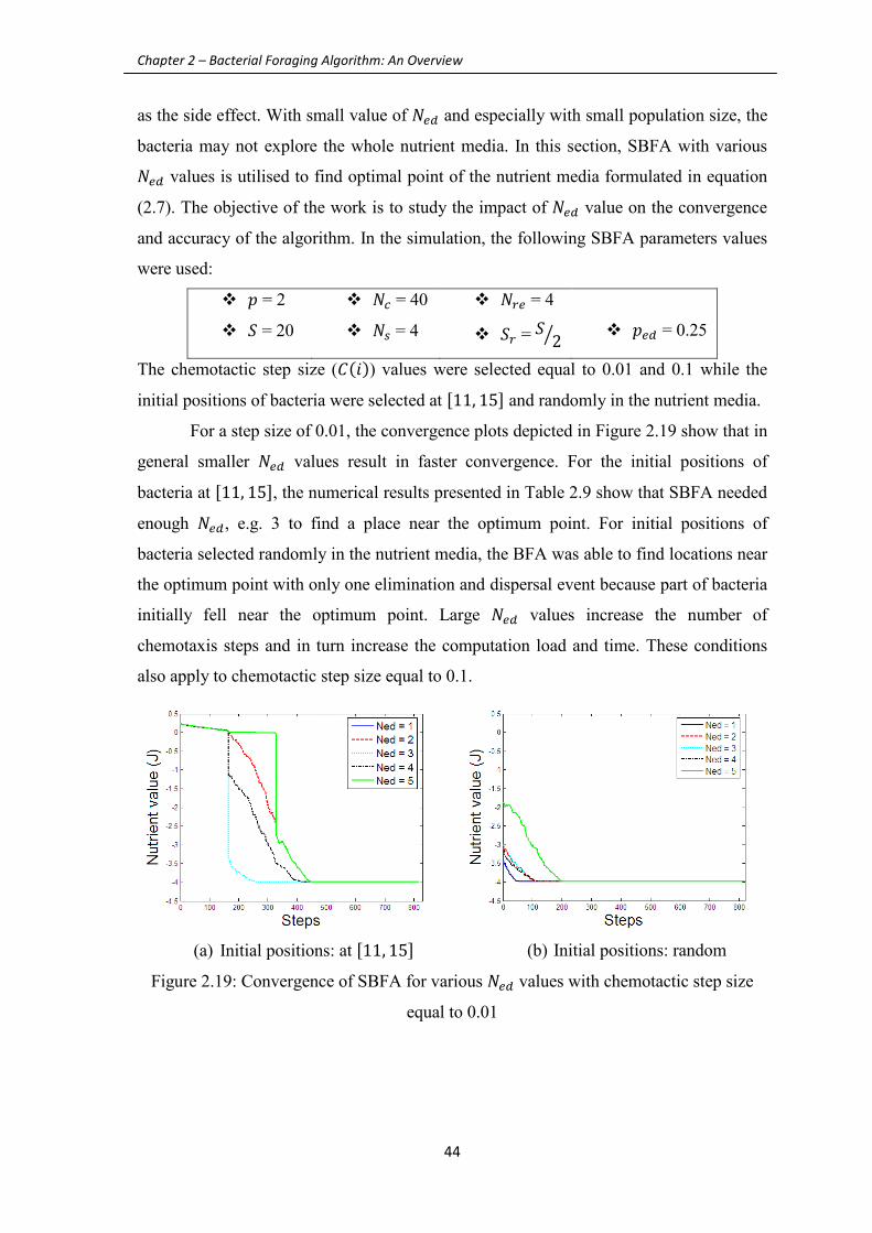
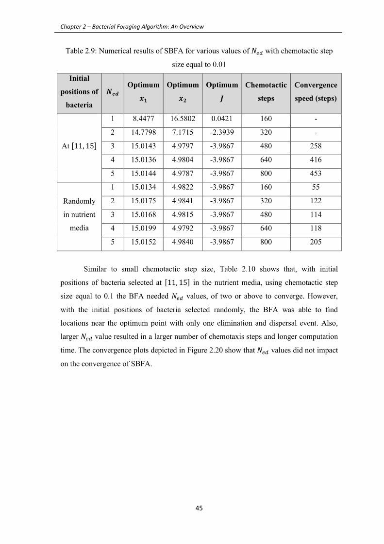


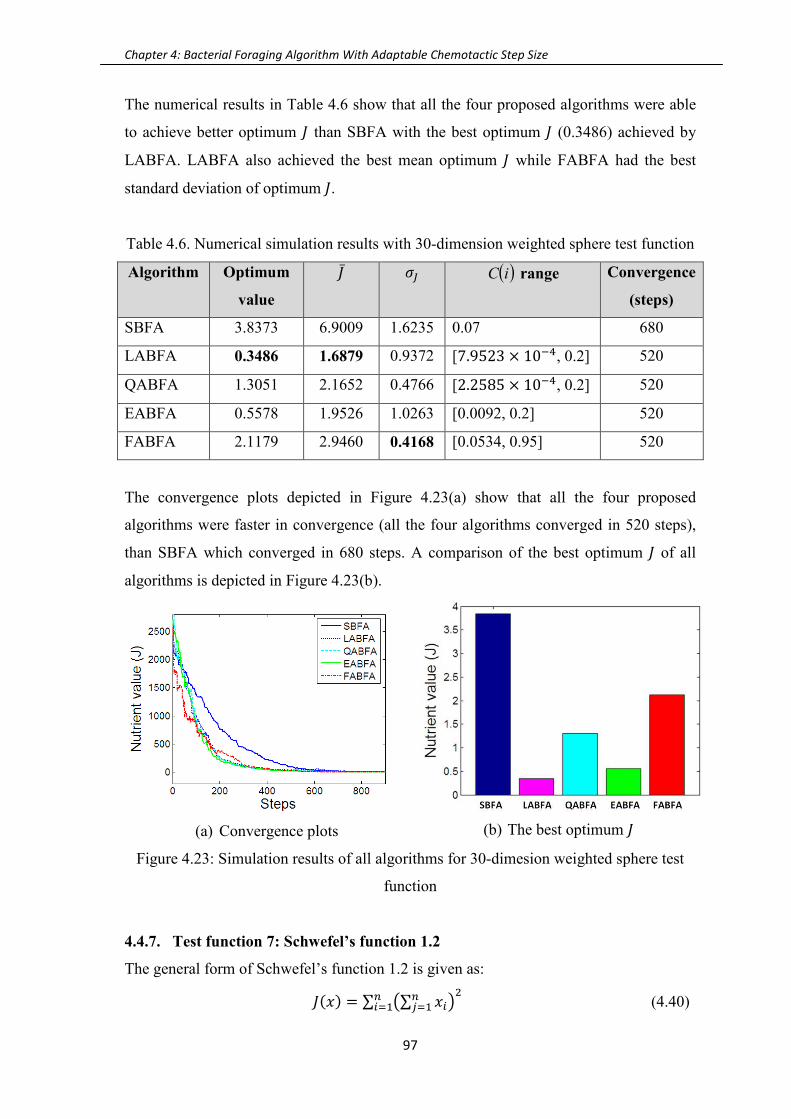
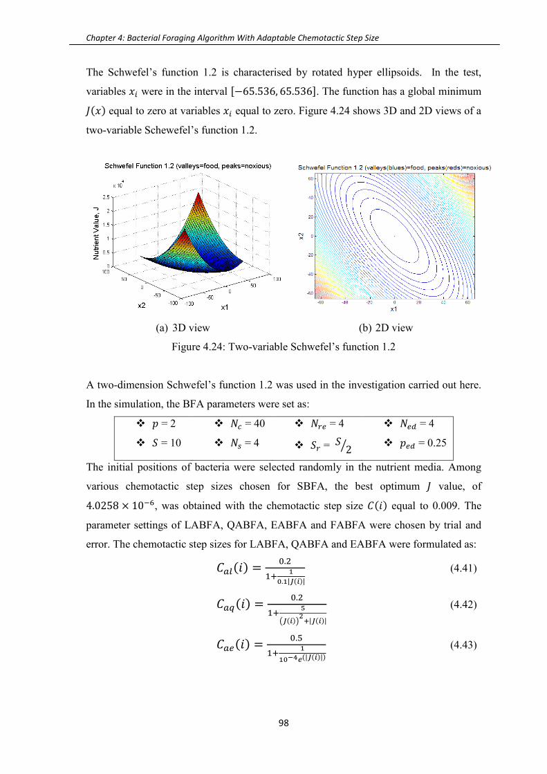


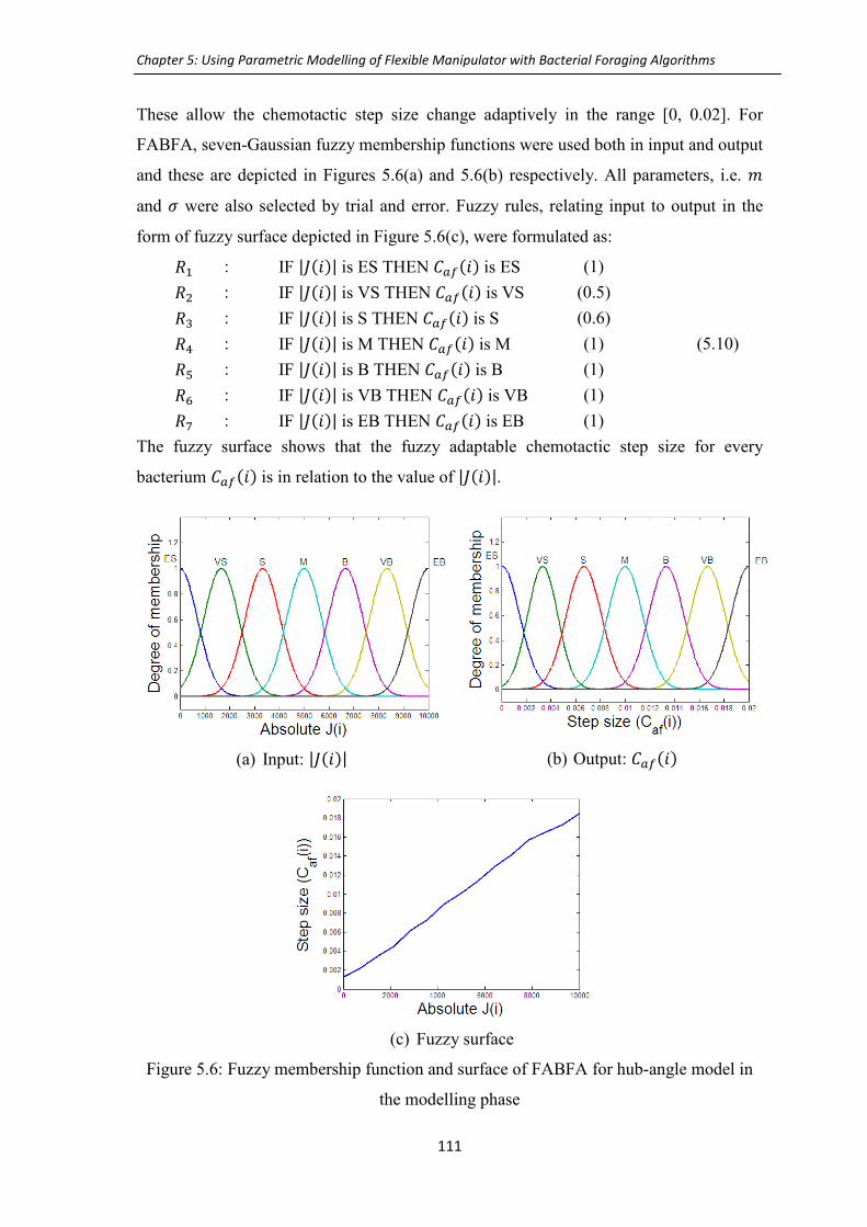

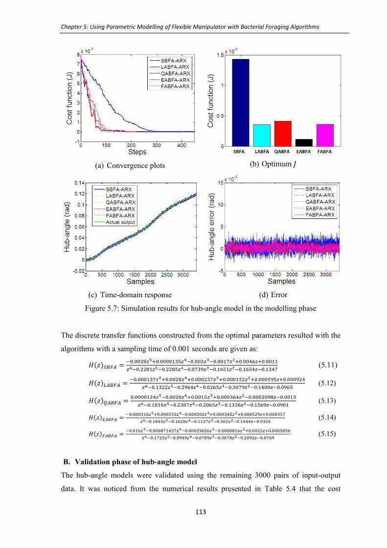

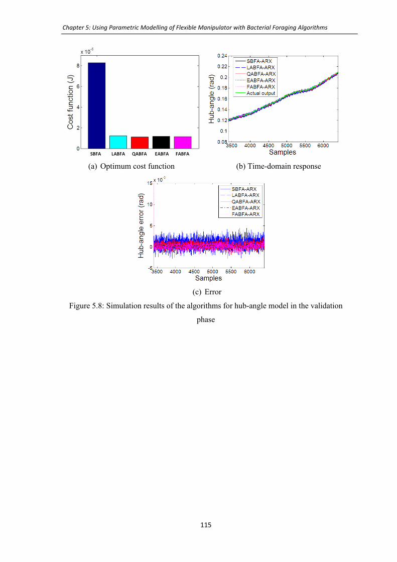


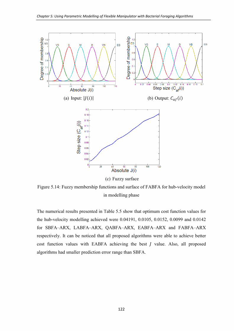


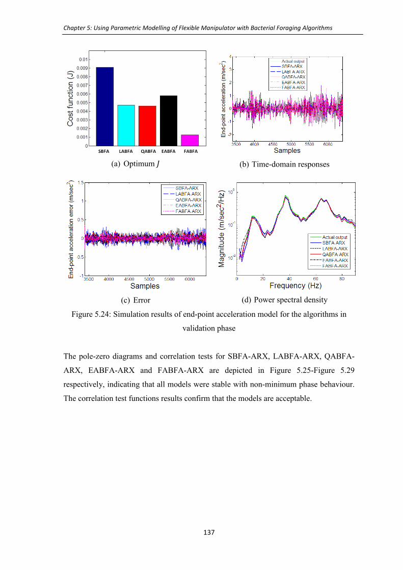


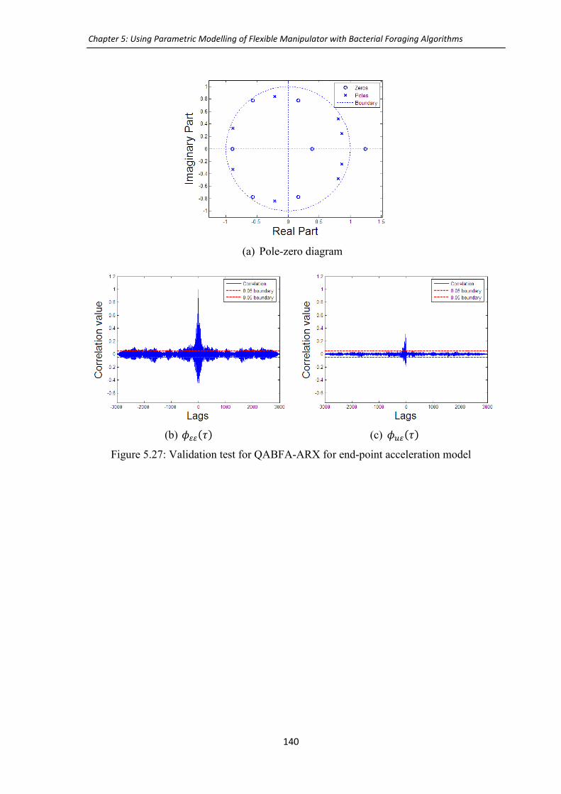

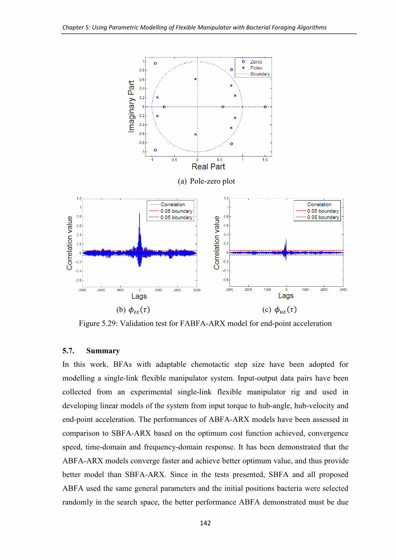


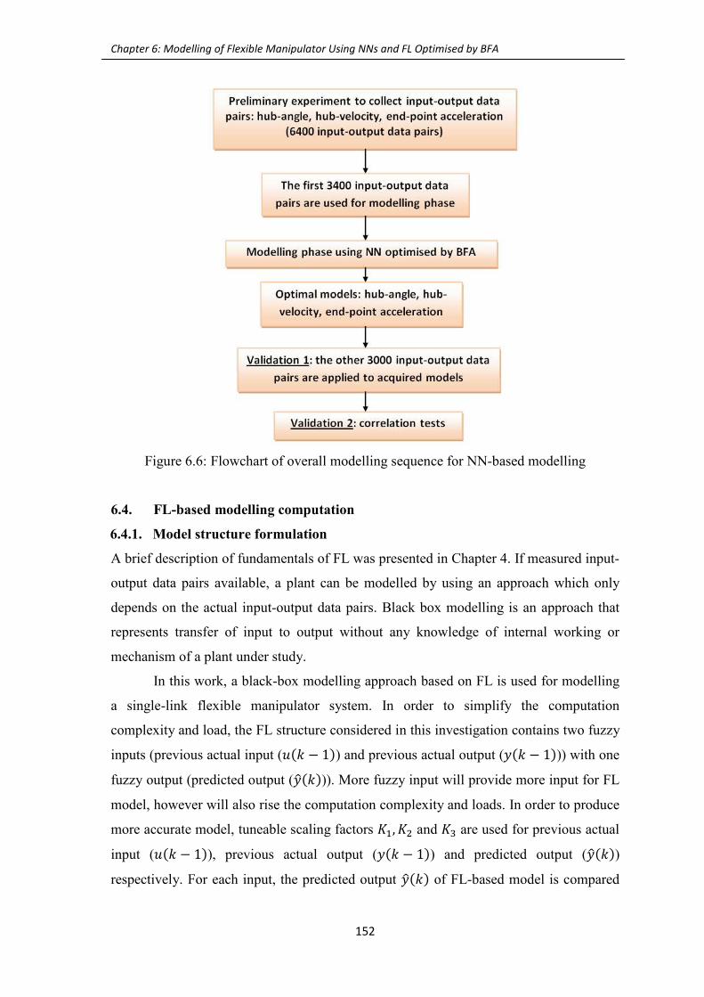


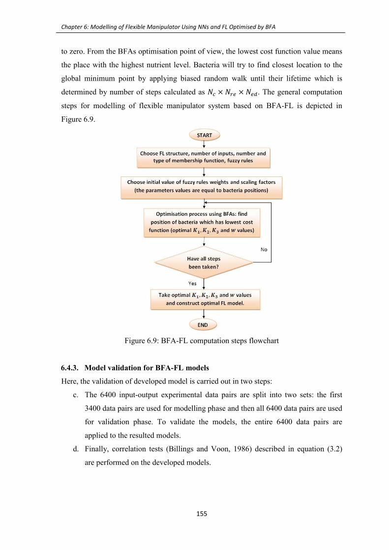


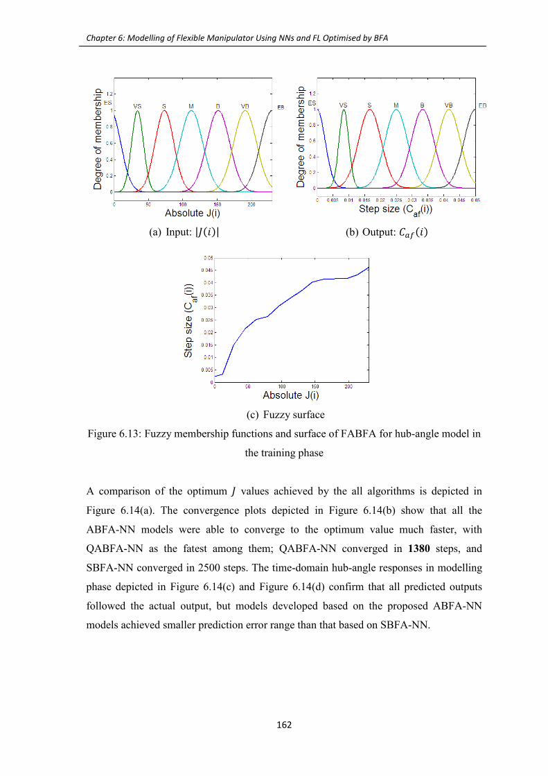


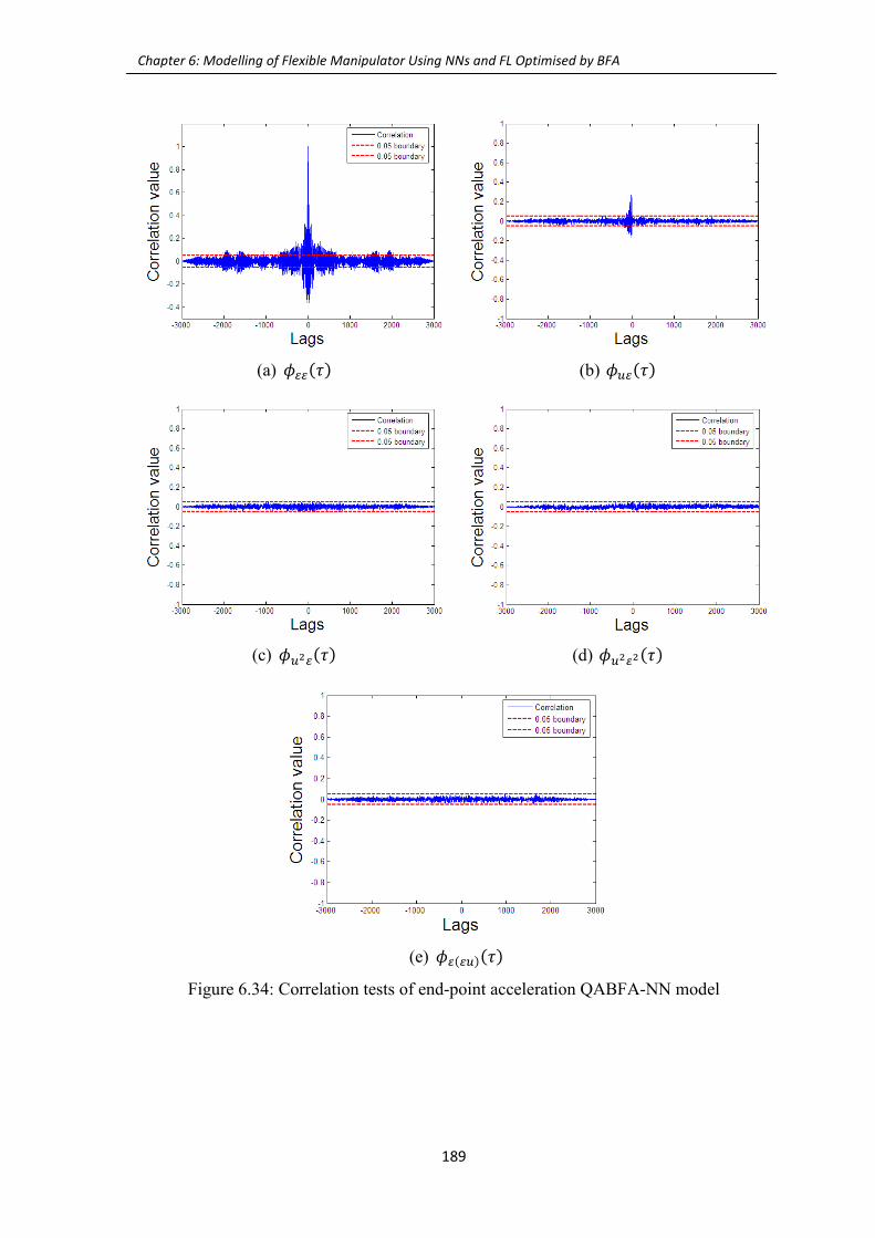


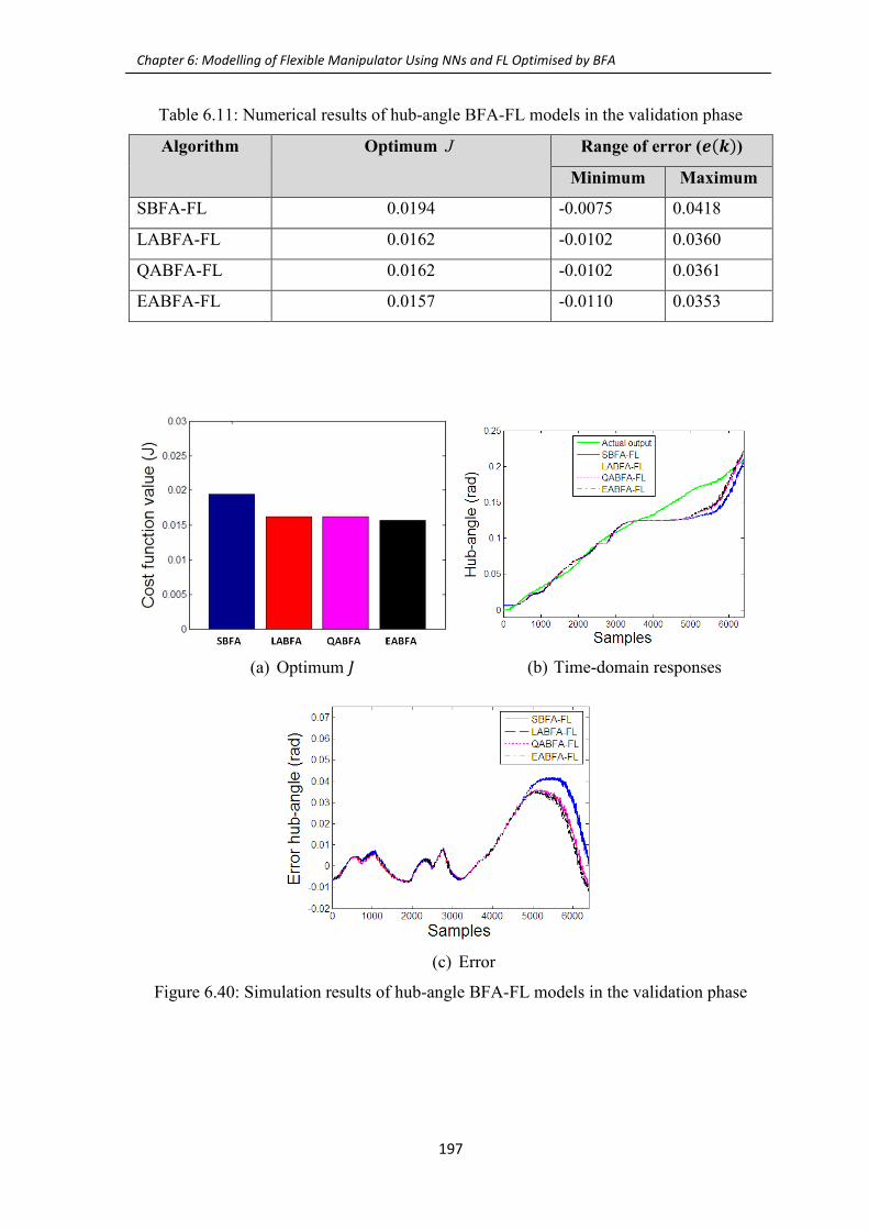


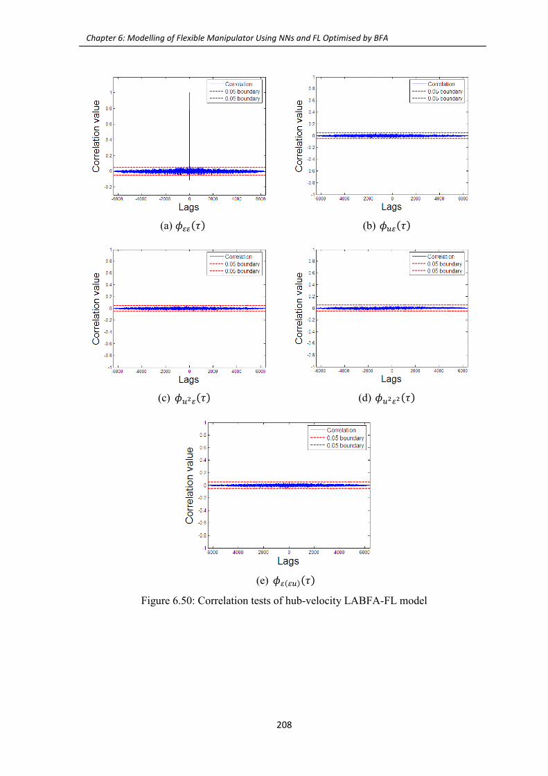
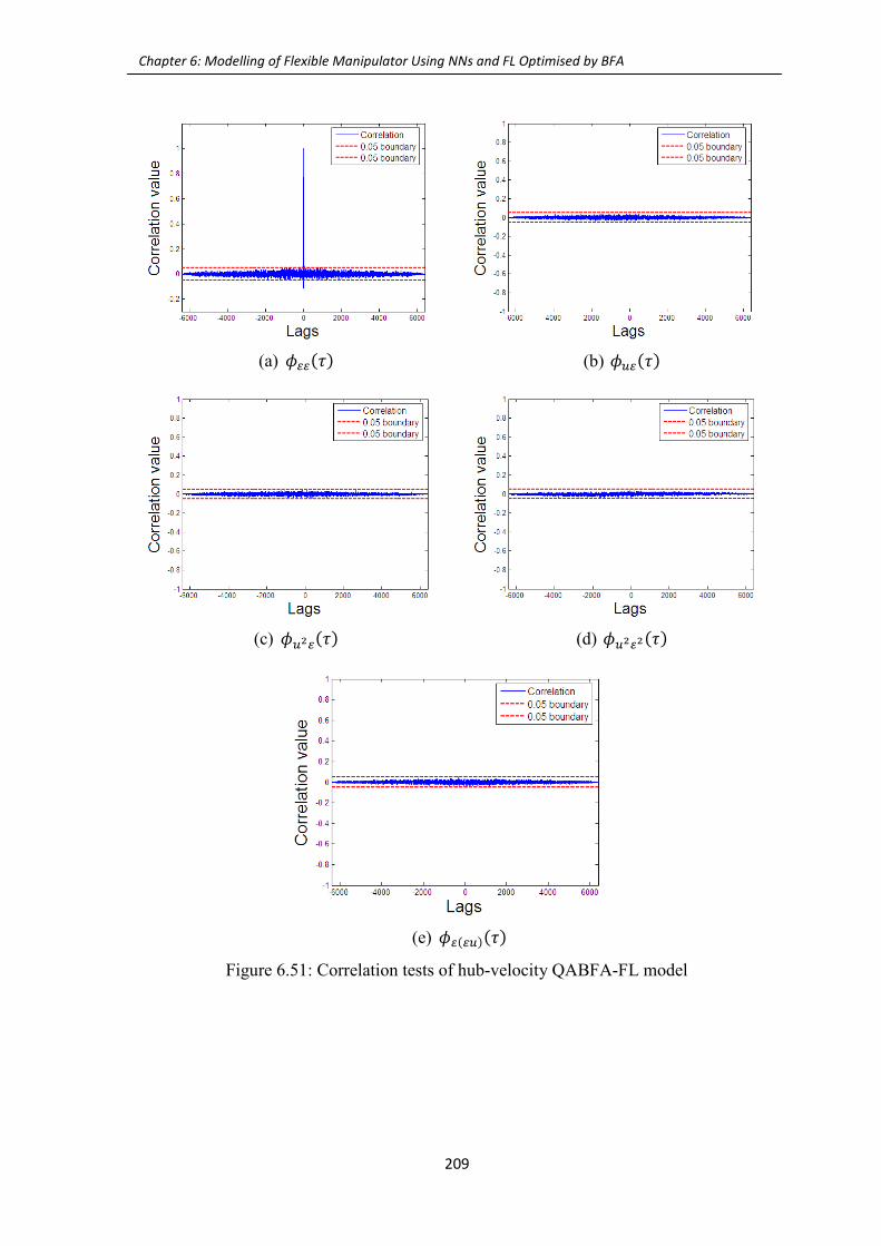


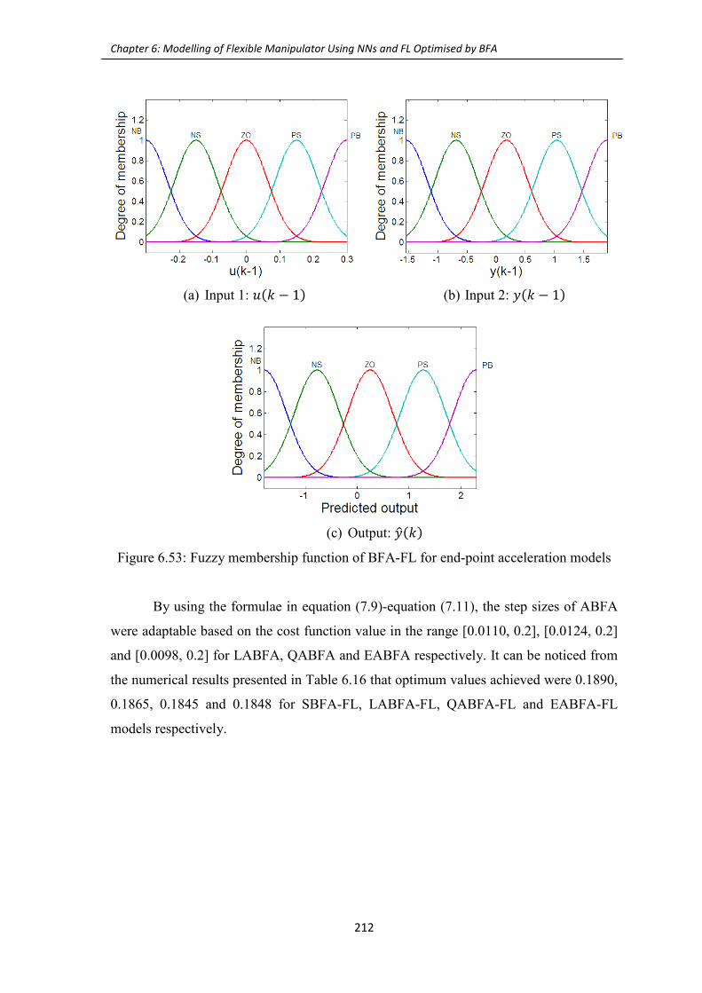


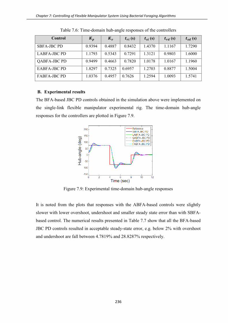

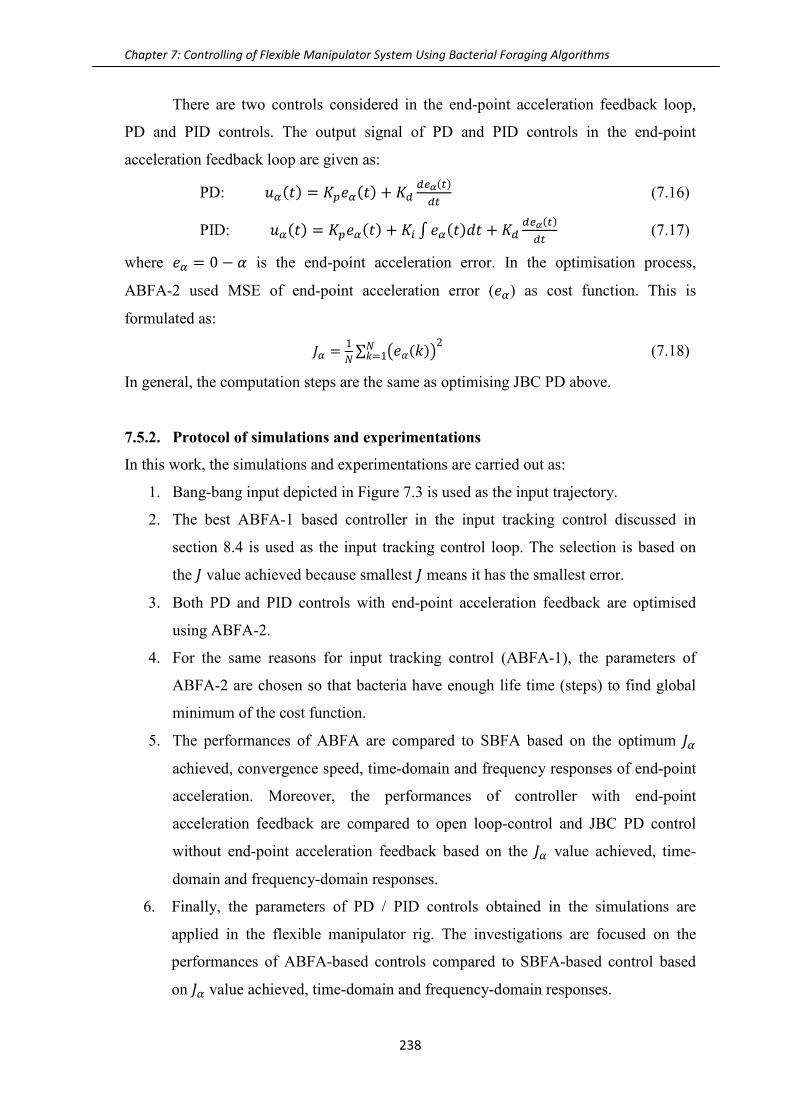


![PLATINUM SPONSOR - Closte · LEVEL OF SPONSORSHIP [CHECK ONE]: q PLATINUM SPONSOR [$10000] q GOLD SPONSOR [$5000] q Breakfast Sponsor q Lunch Sponsor q Gift Sponsor q Auction Sponsor](https://static.documents.pub/doc/80x56/60014c66d50c102c412072c5/platinum-sponsor-closte-level-of-sponsorship-check-one-q-platinum-sponsor-10000.jpg)


