Cube Data in the VO – V0.3, May 6, 2013 Access to Multidimensional (Cube) Data in the VO Use Cases, Analysis, and Architecture PREPARED BY ORGANIZATION DATE Douglas Tody NRAO April 15, 2013 Arnold Rots SAO Bruce Berriman IPAC Mark Cresitello-Dittmar SAO Matthew Graham Caltech Gretchen Greene STScI Robert Hanisch STScI Tim Jenness Cornell Joseph Lazio JPL Omar Laurino SAO Raymond Plante NCSA Change Record VERSION DATE REASON 0.2 Apr 30, 2013 Revised use case section, new intro/req section 0.3 May 6, 2013 Changes in response to review comments
Transcript
Cube Data in the VO – V0.3, May 6, 2013
Access to Multidimensional (Cube) Data in the VO
Use Cases, Analysis, and Architecture
PREPARED BY ORGANIZATION DATE Douglas Tody NRAO April 15, 2013 Arnold Rots SAO Bruce Berriman IPAC Mark Cresitello-Dittmar SAO Matthew Graham Caltech Gretchen Greene STScI Robert Hanisch STScI Tim Jenness Cornell Joseph Lazio JPL Omar Laurino SAO Raymond Plante NCSA
Change Record
VERSION DATE REASON 0.2 Apr 30, 2013 Revised use case section, new intro/req section 0.3 May 6, 2013 Changes in response to review comments
Cube Data in the VO – V0.3, May 6, 2013
Table of Contents Executive Summary...................................................................................................................... 1 1. Introduction ........................................................................................................................... 2
1.1. Usage Context............................................................................................................................... 4 1.1.1. Data Product Types................................................................................................................. 4 1.1.2. Operations, Processing, and Analysis..................................................................................... 4
3.3. VO Protocols .............................................................................................................................. 15 3.3.1. SIA Version 2 ....................................................................................................................... 16 3.3.2. SIAV2 AccessData ............................................................................................................... 18 3.3.3. TAP, ObsTAP, Data Linking................................................................................................ 21
3.4. Image Data Model...................................................................................................................... 22 3.4.1. Abstract Model ..................................................................................................................... 23
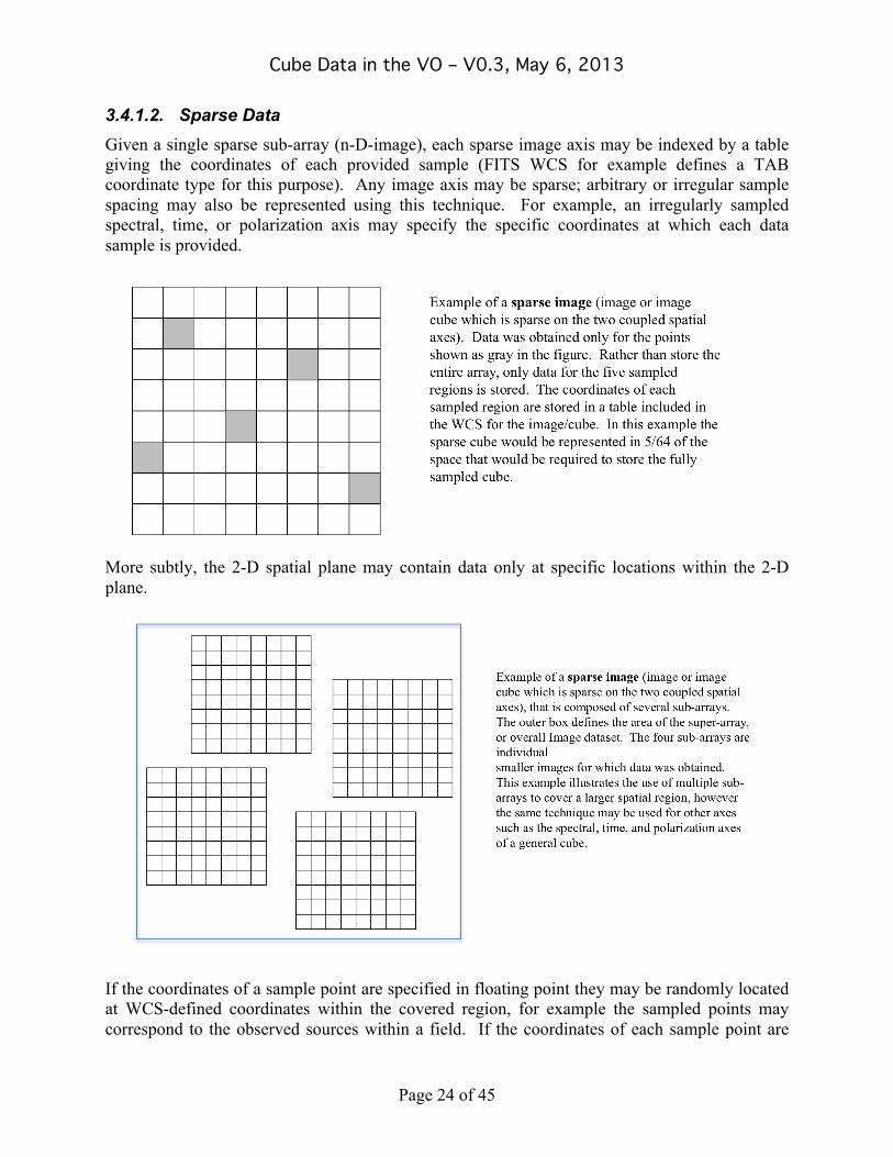
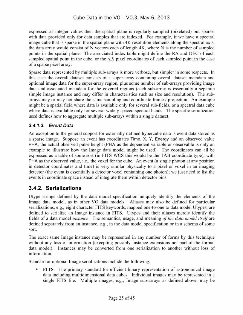
3.4.1.1. Hypercube Data .............................................................................................................................23 3.4.1.2. Sparse Data ....................................................................................................................................24 3.4.1.3. Event Data .....................................................................................................................................25
6. Appendix: Use Case Analysis ............................................................................................. 28 6.1. Categories of Use Cases............................................................................................................. 28
6.2. Specific use cases........................................................................................................................ 30 6.2.1. From Joe Lazio (JPL) ........................................................................................................... 30 6.2.2. From Arnold Rots (SAO/CXC) ............................................................................................ 30 6.2.3. From Doug Tody (NRAO) ................................................................................................... 31 6.2.4. From Eric Keto (SAO/SMA) ................................................................................................ 32 6.2.5. From Gretchen Greene (STScI) ............................................................................................ 33
Cube Data in the VO – V0.3, May 6, 2013
6.2.6. From Tim Jenness (Cornell) ................................................................................................. 33 6.2.7. From Ian Evans (SAO/CXC) ................................................................................................ 34 6.2.8. From Jonathan McDowell (SAO/CXC) ............................................................................... 35 6.2.9. From Chris Beaumont (Harvard, Alyssa Goodman's grad student) ..................................... 36 6.2.10. From Bruce Berriman (IPAC) ............................................................................................ 36 6.2.11. From Matthew Graham and Ashish Mahabal (Caltech/CACR)......................................... 37 6.2.12. From Rick Wagner (SDSC)................................................................................................ 37
7. Appendix: Related VO Technology ................................................................................... 38 8. References............................................................................................................................. 41
Cube Data in the VO – V0.3, May 6, 2013
Page 1 of 45
Access to Multidimensional (Cube) Data in the VO
Executive Summary Support for access to multidimensional or “cube” data has recently been recognized as a high science priority by both the IVOA and the US VAO (due to time pressures the study presented in this whitepaper was limited to VAO partner organizations). A wealth of cube data are already available within the astronomical community, with more being produced all the time as new instruments come online. Within the US, new radio instruments such as ALMA and JVLA are already in operation, routinely producing large radio data cubes. Cube data will play a major role for JWST, and is already routinely produced by existing O/IR instruments such as IFUs. LSST and similar synoptic survey telescopes will produce multi-color time cubes. Event data from Chandra and other X-ray telescopes can be considered another form of cube data. Cube datasets are often very large and may be too large to be practical to download for local analysis. Visualization and analysis of large cube datasets, while still driven from the astronomer’s desktop, must often be performed on data stored remotely. Distributed multiwavelength analysis of large datasets stored remotely is central to what VO is all about; hence cube datasets are a natural place to leverage VO technology. However, while VO has much relevant technology to bring to bear, there are currently no VO protocols suitable for publication of and access to cube data. The problem is becoming critical; the community will find other solutions if VO does not provide a solution soon, within the next year if not the next few months. To be adopted by the community the approach will need to be perceived as something that can be implemented rapidly with limited resources.
To begin to address this problem we collected a number of use cases from projects within the US, garnered from radio, X-ray, optical/NIR, and sub-mm, ranging from imaging to spectra, time series, and event data. A use case analysis was performed to derive a number of usage and functional requirements. These were then contrasted against the current and planned VO architecture to determine what will be required to address the issues of cube data.
Our use case analysis was broken into three areas: data discovery, data access, and data usage, i.e., visualization and analysis.
For data discovery, the query needs to be expressive enough to describe a complex region in parameter-search space, limiting the search to the kind of data services required by the client application. While physical data products need to be discoverable, a higher level of abstraction is required to describe very large cubes or wide-field survey data where the physical data products may be too complex or project-specific to be exposed directly. The discovery query needs to be able to describe virtual data products that will be generated on demand if retrieved, to automate access to idealized subsets of large datasets, particularly when posing the same query to multiple data sources. Data access includes simple retrieval of entire cube datasets, but direct access to large remote cubes requires the ability to repeatedly access the same cube dataset directly, to filter, subset, or transform the data, including computing subcubes, slices, 2-D projections via various algorithms such as sums or moments, 1-D extractions, and arbitrary reprojections. Very large cubes may be stored as many small files but are best presented externally as a single large logical entity.
Cube Data in the VO – V0.3, May 6, 2013
Page 2 of 45
Data usage requires that data be described via a standardized abstract data model to provide interoperability; the data model should be extensible to support domain- or provider-specific semantics. Client software varies in the data formats supported. FITS is the defacto standard and must be supported, but optional support for other formats (HDF5, CASA image tables) is desirable. Ideally the data format requested by the client may differ from the form in which the datasets are stored, with the service supplying data in the requested format upon demand.
The VO standards most relevant for cube data access are TAP and ObsTAP (table access, archive data product indexing), SIAV2 (image/cube data access), and data linking (linking data products in the query response to related data products or services). An Image data model (ImageDM) is currently in preparation, with the goal of defining a general abstract data model for multidimensional cube data, defining the data model independently of serialization so that multiple data formats can be supported. This is expected to be FITS-compatible but not limited to just FITS.
Implementation. Our opinion is that while we ultimately need all of these standards, the most critical for supporting cube data are SIAV2, the ImageDM, and data linking. ObsTAP is desirable to support archive browsing and to provide a higher-level view of the available data products, but was designed to provide a generic uniform index of archive data products hence is not well-suited to provide the level of abstraction required to describe large, complex cube datasets, or wide-field survey data where the individual data products may not even be exposed. TAP and ObsTAP are also quite complex in terms of both implementation and usage, and uptake by the community has been slow; if we wait for the community to implement TAP before addressing cube data access we may fail to deliver the required cube data access capability in time. SIAV2, already existing in working draft form and building upon the successful and widely implemented SIAV1, provides a single protocol focused on discovery of and access to multidimensional cube data. The ImageDM can be fully integrated, including data access semantics for automated virtual data generation and client-directed slicing and dicing of large cube datasets, and support for the more advanced use cases such as sparse data. Implementation of SIAV2 support for cube data can begin during the prototyping phase within a matter of months, providing an immediately useful capability that can grow in functionality as it is used for applications such as cube visualization and analysis. The fact that it is a single protocol still under development will make it much easier to add new capabilities, as compared to trying to coordinate development of multiple protocols being developed by different groups (the latter activity could still go forward in parallel, with the goal of normalizing multiple standards 1-2 years from now).
Conclusions. VAO has concluded that a viable approach that meets current science needs, allows us to engage the community quickly, is readily expandable in the future, and has a low barrier to implementation is SIAV2.
1. Introduction Both the IVOA and the USVAO) have recently endorsed support for cube data as a priority for the next 1-2 years of development. By cube data we refer to multidimensional data (n-D images, hypercubes, n-cubes, or for simplicity just “cubes”). Such data may record the spatial, spectral,
Cube Data in the VO – V0.3, May 6, 2013
Page 3 of 45
time, and polarization characteristics of incoming photons; a 2-D image is a special case of cube data with fixed values for all but the spatial axes. Cube datasets are becoming much more common with modern instrumentation and is currently not yet adequately addressed by the VO, hence is a logical choice as a high priority for future development. The following text from the current VAO program plan presents the motivations and context for the cube initiative:
Almost all of our information about the Universe comes in the form of photons. In turn, the properties of photons that can be measured and from which information can be extracted are polarization, direction of arrival, energy, and time of arrival. The most general astronomical measurement therefore is five-dimensional, though specific measurements are often lower dimensional. As examples of the range of different kinds of measurements, a single image represents a simple two-dimensional data set: intensity as a function of position on the sky. The image itself, of course, is acquired for a specific passband at a specific epoch, which are important meta-data that must be captured for full exploitation of the image data. More complex examples could include a search for a spectral line or lines toward a star forming region or a group of galaxies, using the proper motions of masers around evolved stars to track their evolution, or searching for accretion events within young stars in a star forming region. The first example is an illustration of a three-dimensional velocity cube, i.e., intensity as a function of position and velocity or frequency; the second example is an illustration of a four-dimensional data set, i.e., intensity as a function of time for a range of velocities or frequencies; and the third example is also an illustration of a four-dimensional data set, i.e., intensity as a function of both time and energy or wavelength.
The need for representations of and manipulations of multi-dimensional data sets is not new, but new facilities will present increasing challenges. For some time, both radio and X-ray instruments effectively have produced at least three-dimensional data sets (e.g., image cubes of intensity as a function of position and frequency or photon direction of arrival as a function of energy). With the advent of facilities such as the Jansky Very Large Array (JVLA), the Low Frequency Array (LOFAR), and the Atacama Large Millimeter/submillimeter Array (ALMA), though, the size of the image cubes is expected to increase dramatically. Similarly, integral field units (IFUs) on optical and near-infrared cameras are becoming widespread, and the James Webb Space Telescope (JWST) will naturally deliver spectral data cubes. Further, all of the radio instruments are also naturally capable of delivering polarized velocity cubes, i.e., velocity cubes for multiple polarization vectors. Similarly, time domain astronomy is entering a new era. The Large Synoptic Survey Telescope (LSST) will produce five-color images every 15 seconds, naturally resulting in four dimensional image cubes on the sky. Many of the new radio facilities, those listed above and the Square Kilometer Array (SKA) Precursors, have time domain searches or projects as part of their key science programs.
This whitepaper was prepared to examine the problem of cube data at a high enough level to engage the broader community, beyond just those involved in developing the IVOA standards. We examine the challenges posed by cube data and examine current and planned elements of the VO architecture to see how well they meet the requirements posed by cube data. A number of use cases of cube data contributed by individuals and projects within the broader community are included (6) in order to better define the problem to be solved.
Cube Data in the VO – V0.3, May 6, 2013
Page 4 of 45
1.1. Usage Context The access and analysis of data cubes can be divided into several facets, which encompass both the data products and the analyses that can be applied to such products.
1.1.1. Data Product Types Domain specific data products: This category includes waveband, instrument, and/or configuration-specific data products, including calibration files, visibility data, un-calibrated event lists, and so forth. Metadata are usually observatory-specific and not standard. These products need specific expertise in order to be handled in a scientifically meaningful way.
Standard n-cubes: Domain-specific raw data products may be processed by pipelines (or reprocessed by users) to create standard n-dimensional hypercubes or “n-cubes”. A FITS image of dimensionality N is a simplified instance of an n-cube where the data samples are expressed as an N-dimensional numeric array to optimize storage and computation. The elemental component of a standard n-cube is a voxel, i.e., a discrete element in the n-dimensional space determined by the “n” quantities measured by the instrument. The voxel’s value occupies a hypervolume defined by the pixel size along the different axes, and may be characterized by resolutions and statistical errors or upper/lower limits. In some cases, multiple physical axes may be collapsed onto a single, degenerate n-cube axis (e.g., the spatial/spectral data axis from a slitless spectrograph or single-pixel axes). Standardized metadata express the position of the reference pixel or voxel, the projection of the voxels, the units, and any other information useful to make scientific sense of the data. The metadata also may reference the raw data products and the processing history of the n-cube. Using and analyzing these standard n-cubes usually does not require domain-specific expertise. However, specific expertise is definitely required in order for the user to be able to regenerate standard n-cubes from the original raw data files. Abstract data model: While the raw data and metadata are likely to follow customized data models, an abstract representation of standard n-cubes is required in order to allow interoperability. An Image data model (3.4) is currently in preparation within the IVOA to provide this standard model, focused initially on multidimensional astronomical image data, e.g., FITS images and cubes, although some support for generalized n-cube data such as event lists is also provided.
The mapping between the abstract data model and the actual n-cube realization such as is stored in an archive will require low-level I/O software for interpreting the data file, and a higher-level layer on top of that for mapping the file contents to the abstract data model. VO data access protocols (3.3) and their realization as data services for a specific archive will provide a standard interface for client applications to directly access cube data stored in archives, without need to download an entire dataset or understand the physical form of the data as stored in the archive.
1.1.2. Operations, Processing, and Analysis Common operations on n-cubes: Some operations can be performed on any standard n-cube, using generic standard tools. This list is somewhat arbitrary, but in general these operations should not depend on any domain specific information. Such operations may include:
Cube Data in the VO – V0.3, May 6, 2013
Page 5 of 45
projections over a set of axes, aggregation of voxels along one or more axes (e.g., average, median, sum), extracting sub-arrays, and interpolation.
More sophisticated analysis algorithms include derivation of moments along specific axes, pattern recognition, feature extraction, and cuts along arbitrary surfaces. Some of the operations can lead to other publishable products: 1D signals (e.g., spectra, time series, SEDs), 2-D (e.g., images, visibility maps, polarization maps), and possibly higher dimensions (e.g., 3-D SEDs with spectral, flux, and time axes). Common operations can be applied to these derived products (e.g., cross- and auto- correlations, phase analysis for 1D signals; source detection and photometry for images; fitting/modeling in the n-D space). Standard metadata also allow one to consistently display n-cubes, their projections, and their derived products.
Custom operations on n-cubes: Some operations can be specific to a science domain or to a particular energy band. Experts must be able to perform these operations in the specific domain on the standard n-cubes themselves, without requiring any additional information. For example, if the n-cube contains data about an object of a specific class, then domain-specific analyses can be performed (e.g., photometric redshift estimation for AGN).
Reprocessing of the raw data: Users might be interested in reprocessing the raw data by applying domain-specific operations on them. Domain-specific tools could allow one to annotate the resulting products with standardized metadata and according to the standard data model. Access to, and analysis of, raw data can be performed using customized protocols, data models, and metadata descriptions, since specific understanding of these components is required. However, the standardization is in the creation of the derived products that can then be used by standard applications, along with data coming from standard services/applications. A common example of custom reprocessing is where the user, possibly working remotely, reruns the pipeline processing for the dataset using custom processing parameters specified by the user.
Republishing of derived data products: Derived data products, generated by standardized applications, can be republished via data publication services, becoming part of a derived, annotated knowledge base associated with the data. Data Flow: A data product’s life cycle will generally follow this path:
Observation – pipeline domain-specific products – processing VO n-cube – analysis derived products – further interpretation – publish VO or elsewhere.
2. High Level Requirements Putting it all together — discovery, access, and usage of large data cubes: Data discovery allows the user to find out what data are available in a specific region of the high-dimensional space that represents the observed parameter space. Parameters are not only the coordinate axes in the (space, time, spectral, redshift, polarization, etc.) domain, but also include additional technical parameters that may be relevant, such as the desired instrumental resolution and accuracy, calibration properties, and so forth.
So, a query to a discovery service needs to be expressive enough to represent the complexity of the region in this parameter space, and must not assume that the ROI boundaries are parallel to
Cube Data in the VO – V0.3, May 6, 2013
Page 6 of 45
the parameter space axes. The query must also allow the user to narrow the search down to the kind of data services of interest (e.g., mosaic, cut-out, and so on).
Data access: Access to the chosen data products must be provided in an efficient way. Since we may be dealing with very large datasets, sometimes in the Terabyte range for a single cube dataset (6.2.3), downloading entire large cubes for local access may not be feasible. Direct access to large cubes stored remotely is required, allowing repeated access to dynamically computed subsets or views of the remote cube. Abstraction is also required so that the client application does not need to understand the details of how the remote dataset is represented: very large cube datasets may be physically stored in a complex structure composed of multiple smaller files, that may still be viewed logically by the client as a single cube dataset.
Data model: Having a standard means to discover and access data products has little value if the discovered data products require specific expertise in order to be meaningfully used. If an astronomer needs to study the documentation of each data access service to understand how to use the products, then they might as well use the local custom access interface instead of a standardized one. So, it is important that the cube datasets are provided in a standard format, via standardized interfaces. It is not feasible for a single abstract data model to adequately describe all astronomical cube data, hence, it must be possible to extend the abstract data model and describe the extensions in a standardized way, so that data providers can convey domain-specific information to more fully describe the characteristics of their data. Data formats: While the abstract data model defines the semantic content of a cube, actual data might come in different formats. In general the choice of a data format may depend upon matters such as the complexity and size of the dataset to be represented, how the client software will use the data, and what file formats are supported by the client. It is possible to serialize the same cube dataset in various formats without loss of information (except possibly nonstandard extensions).
While it is not ruled out to define a new data format, it is useful to review the file formats that are commonly used for storing data cubes. The most used formats, at the moment, seem to be:
• FITS • HDF5 • CASA Image Tables • VOTable (for metadata in VO queries)
These formats have been designed following different approaches. FITS provides a standard representation for multidimensional cube data as well as table data, and is currently the most widely used such format in use within astronomy. HDF5 and CASA image tables (or more generally the CASA Measurement Set) have been adopted because of their ability to store large complex datasets. However, they are quite different; for example, HDF5 employs a hierarchical model, while CASA image tables use a more flexible relational model similar to FITS. A thorough comparison between these two formats (although from CASA perspective) is provided in http://www.astron.nl/~gvd/tables-hdf5-comparison.pdf. A comparison of the first three formats in the context of a remote data visualization use case is provided by Kitaeff et al. (http://arxiv.org/pdf/1209.1877v1.pdf). An analysis of cube data formats from the
Cube Data in the VO – V0.3, May 6, 2013
Page 7 of 45
perspective of the proposed VO Image data model is presented in section 3.4.2 of this whitepaper.
2.1. Usage Requirements We have analyzed the use cases accumulated to this point (6) and come up with the following high level user requirements:
• The protocol has to allow for searching for a location within a cube. The location can itself be a cube.
• The protocol has to allow for the extraction of sub-cubes of lower dimensionality from a parent cube.
• The protocol has to allow for the cube to have gaps in one or more dimensions, that is, it must provide efficient support for sparse cubes.
• The query interface has to allow for translation between native units of cube and "natural" units for the user. (e.g., the user can enter a velocity range, relative to the LSR, even if the cube is stored in Hz.).
• The protocol has to allow for non-linear mappings to world coordinates from the axes of the cube.
2.2. Functional Requirements Analysis of the usage requirements and the more detailed use cases results in the following high-level functional requirements. This is not intended to be an exhaustive list; rather we try to list the major capabilities required and especially any which are less obvious. We refer to a query or data access posed to an “archive”; this is the simplest and most common case but actual data discovery and access need not be limited to this case, e.g., in global data discovery an aggregation service might instead be queried, or the service to be queried might provide data from a theoretical model, with data products generated on demand from the model.
1. Data Collections a. Provide access to conventional individual cube data products, including 2-D
images as well as higher dimensional cubes with any combination of spatial, spectral (including velocity and redshift), time, and polarization axes. [This is the conventional case of access to an explicit, well-defined image/cube data product of reasonable size.]
b. Provide access to complex cubes that may not be represented as conventional data products in an archive, e.g., a very large cube stored as many files, possibly in some arbitrary collection-specific internal format such as a database, that is viewed externally as a logical cube data product. [Derived requirement: distinguish the logical or external view from how the cube datasets are physically represented as data products within an archive.]
c. Provide access to wide-field survey data with complex coverage. Such data may cover a large region; it may be simple 2-D imagery or it may be higher dimension
Cube Data in the VO – V0.3, May 6, 2013
Page 8 of 45
cube data, e.g., spectral or time cube data possibly with polarization. [Derived requirement: allow the client to specify the ideal data product it would like to get back given only collection-level knowledge of the data, with the service to respond with a description of what it can actually return. This case includes on-demand generation of data products from a theoretical model.]
d. In the most general sense, event datasets are a form of (hyper)cube data. Provide optional support for direct access to event data so that suitably capable applications may perform analysis at the level of individual events. [Generic applications should have access to an already imaged version of the data. Visibility datasets are also a form of hypercube data, but the data volume and Fourier transform required to image the data generally require that VO-level analysis be performed in the image domain.]
2. Data Discovery
a. Provide the capability to discover the physical cube data products stored in an archive [this is the case where one merely exposes static data products stored in an archive, with a discovery query listing those that match the query constraints.]
b. Provide the capability to discover virtual data products that can be generated from the data available in an archive [in this case the client describes the virtual data product it would ideally like to have, and the service describes what it can actually deliver; this is required for at least case 1c above.]
c. It shall be possible to query by the physical coverage in which data are desired (spatial, spectral, redshift/velocity, time, polarization), by the characteristics of the data (resolution, calibration level, etc.), or by other characteristics such as target name, well-known dataset identifier, publication reference, and so forth. [That is, query by standard VO metadata.]
d. It shall be possible to query by collection- or service-specific extension metadata specific to the archive [VO queries posed to standard data models and standard metadata are necessarily generic, but queries posed to a specific archive can be much more useful if extended by collection-specific metadata.]
3. Data Description
a. In a discovery query, the query response shall describe each available physical or virtual cube data product in sufficient detail to allow the client to decide in scientific terms which available datasets to retrieve for subsequent analysis [this is hard to specify or ensure, but essentially it means populate the metadata for the standard VO data models, plus optionally provide extension metadata specific to the individual data collection.]
b. In a discovery query, provide metadata sufficient to retrieve the described dataset [e.g., an access URL or publisher dataset identifier that can be used to retrieve the referenced physical or virtual data product.]
c. In a discovery query, provide metadata sufficient to plan direct access to the described dataset [describe the data quantitatively in sufficient detail to allow the
Cube Data in the VO – V0.3, May 6, 2013
Page 9 of 45
client to do directed access, e.g., project, slice and dice, etc. the dataset, in either WCS or pixel/voxel coordinates.]
4. Data Retrieval a. The service protocol should provide sufficient information for the client to
retrieve the described cube dataset [e.g., an access URL or publisher dataset identifier uniquely identifying the specific physical or virtual data product.]
b. If the data collection being queried may provide large datasets an estimated dataset size must be provided in the query response [if the described cube is 600 GB we want to know before trying to download it.]
c. The format of the data product to be returned must be specified by the query protocol, or otherwise specifiable by the client upon retrieval [ideally it should be possible for the client to specify the data format in which it would like to receive data, with the service doing the translation if necessary.]
d. Data retrieval must be efficient enough for the client application [this is hard to quantify and very application dependent, but essential if a standard protocol is to be used; in practice it means flexibility in return data formats, optimization of the returned data, e.g., binary or non-verbose encoding, omit the metadata if not required; use compression where appropriate; allow multiple simultaneous requests to be executed in parallel.]
5. Data Access a. It should be possible for a client to directly access (access into) a cube dataset
without first retrieving the data, e.g., to filter, subset, or transform the data on the server side before returning an optimized data product to the client. [This is essential for very large cubes and for complex cube datasets where the logical and physical views are distinguished, but is also useful for things such as many small cutouts of ordinary 2-D images, or access to individual spectral line profiles from multispectral or multiband spectral.] [This is an optional advanced capability, not required for simple discovery and retrieval of static archive datasets.]
b. It shall be possible to filter a cube dataset in the spatial axis (cutout), in the spectral axis (list of spectral regions to be included or excluded), in the time axis (list of time intervals to be included or excluded), or in the polarization axis, to select individual polarization measures to be returned in the case of data observing in multiple polarizations [This includes the capability to extract simple cutouts, subcubes, spectral or time sequences optionally with a background or good time filter, and so forth.]
c. It shall be possible to subset the data by some data summation or averaging of some form, e.g., computation of 2-D projections of a 3-D cube using a specified algorithm (e.g., sum, mean, min, max, simple moments). [This is an optional advanced capability. Some operations, e.g. moment calculation or interpolation, may require non-trivial algorithms; in general we want to permit such powerful operations while leaving the details to the service, since the algorithm used may vary greatly depending upon the domain of the data and the software used.]
Cube Data in the VO – V0.3, May 6, 2013
Page 10 of 45
d. It shall be possible to compute a slice through a cube at an arbitrary position and orientation, with a specified slice width. [The details of how this is best done may be data or software dependent and would be left up to the service.] [This is an optional advanced capability.]
e. It shall be possible to reproject a cube, e.g., compute a new cube with a specified WCS projection, including dimensional reduction if specified. [This is often done for example to match datasets for comparison. Details such as how interpolation is done would be left to the service.] [This is an optional advanced capability.]
f. It may be possible to transform a cube, e.g., by computation of a moment that involves fitting a profile, by computation of the spectral index or curvature, or by computation of domain-specific functions such as a UV-distance plot, rotation measure, time series periodogram, etc. [It is an open question what functionality of this type is appropriate for a data access interface, but some functions are standard enough to be considered, and it is attractive to move such computation to the server, close to the data.]
g. [Comment, not really a requirement] It is also possible to “view” a cube as different type of astronomical dataset, e.g., a Spectrum or TimeSeries via the appropriate VO protocol. However this is not cube data access per se, but rather different types of VO data access being applied to the same underlying multidimensional dataset. One can also extract spectral or timeseries sequences from a cube using cube data access, however the returned object is a 1-D cube. True spectral or timeseries extraction is more complex, involving techniques such as a synthetic aperture, background modeling and subtraction and so forth, and hence is a more complex operation producing an actual Spectrum or TimeSeries data product as the result.
6. Data Usage
a. For a data product returned by a data service to be useful by a client application it must be in a form that the client can (reasonably and affordably) deal with. For common astronomy software this means supporting data formats (e.g., FITS, VOTable, HDF5) and data models (FITS WCS, VO) commonly in use. Evolution and diversity of data representations is good too, hence it is desirable to have the capability to support multiple representations allowing the client to specify the format for returned data products. [Derived requirement: define the abstract data model independently of representation.]
b. The semantic content of a data product is also critical for effective use for client analysis. This involves 1) support for standard data models to enable use of the data product by generic software, 2) support for metadata extension to allow the data provider to extend the standard model to more fully describe their software, both for the end user and for client software which is data-aware, and 3) where appropriate, access to more fundamental data, e.g., event or visibility data, should be provided to permit more sophisticated analysis then may be possible given data that has been rendered to a standard model.
Cube Data in the VO – V0.3, May 6, 2013
Page 11 of 45
3. Architecture Having described the cube data problem, in the following sections we examine the elements of the VO architecture relevant for cube data discovery and access, and describe how these would be used for cube data, to help evaluate possible approaches. We introduce the major components and provide some examples of their use in typical scenarios, then examine each major element in more detail. How to use these elements to construct distributed analysis and visualization applications is examined, including scaling up to Terabyte-sized cube datasets. The primary elements of the VO architecture that we are concerned with here are the following:
TAP Table Access Protocol; provides a general interface that can be used to query arbitrary database tables in any supported DBMS with an SQL-like syntax called ADQL (astronomical data query language).
ObsTAP A generic index to archive science data products or observations, where the Observation Core Components data model (ObsCore) is used to define standard metadata stored in a database table. This can be used to discover simple image/cube data products and associated data, e.g., the instrumental data used to produce the cube data, or any derived data products. ObsCore can be extended with locally defined metadata to more fully describe local data collections such as instrumental data. Data linking can be used to link directly to additional resources (see below).
SIAV2 Simple Image Access protocol, version 2.0 (“simple” means it has a simple mode of usage for static 2-D images, not that it is a simple protocol overall). This provides an object-oriented interface to image and cube data (any multidimensional Image data; hereafter “image” refers to general n-D cube data of which a 2-D image is a special case), based upon the VO Image data model. Capabilities are provided for data discovery, data description, data retrieval, and data access including both automated, scalable generation of virtual data products as well as direct client access to a specific cube dataset via an accessData method. (SIAV2 and the ImageDM are proposed VO standards currently under development; and earlier SIAV1 interface is in wide use).
Data Linking A technique used to link associated data products or services to a given data product. (Data linking is a proposed VO standard currently undergoing development and prototyping).
SAMP Simple Applications Messaging Protocol. Provides a capability for a desktop application or Web application to broadcast, send, or receive messages to/from other applications.
Examples of how these and other VO components are used for cube data access are given in the next section. For a more comprehensive summary of relevant VO technology see section 7. Our purpose here is only to introduce the VO technology with some simple user scenarios; a collection of actual use-cases is given in section 6.
Cube Data in the VO – V0.3, May 6, 2013
Page 12 of 45
3.1. Typical Scenarios In a typical simple scenario a client application may query for and access data using only an image (SIAV2) service. TAP is not required, although having both will provide a richer multilevel query/discovery capability:
• The client application issues a discovery query to the SIAV2 service and gets back a list of datasets (images or cubes) matching the query.
• The list of available datasets is examined on the client side and a decision is made to download or access a particular image dataset. A GUI display could be used to directly download selected datasets, or a SAMP message could be broadcast to display a particular image or cube in the user’s preferred application (CASA viewer, Aladin, DS9, etc.).
• The image referenced in a query response is downloaded via HTTP GET given the access URL returned in the query response. Access may result in on-demand generation of the referenced (“virtual data”) image, or a static (existing) archive file may be returned.
• Alternatively the client application may interactively access the image or cube, using the accessData service operation to successively retrieve portions or views of the dataset.
Note that the simplest use case is always possible, i.e., a query followed by downloading an entire dataset such as an image or smaller cube.
A more complex scenario illustrating how all these elements can work together is as follows: • The user browses data via an archive Web query interface. This could be an archive-
specific custom query interface based upon lower level VO technology such as TAP or ObsTAP, displaying the results of a query (a VOTable) in tabular form in a browser, or it could be the built-in Web query interface from a VO service framework such as DALServer, displaying the results of a query to an ObsTAP or SIAV2 service instance.
• The results of the query display all the data products found that satisfy the specified query constraints. In the case of ObsTAP, any type of science data product can be described, allowing all of the observation-based data products associated with an observation to be displayed, grouped by observation ID. Instrumental data, e.g., a raw or calibrated visibility dataset, as well as derived data products such as an image cube or 2-D projection, are listed.
• The user decides to look at a standard data product image cube for the observation produced by the instrumental processing pipeline. A data link (one of half dozen or so) points to an associated SIAV2 image service that can be used to access the cube.
• The user clicks on the data link and this action causes the application associated with the object pointed to by the link to display something about the data object. For example, the cube is displayed in the CASA viewer, presenting some standard initial view such as a 2-D continuum image for the cube. At this point the application (e.g., CASA viewer) is displaying the remote cube dataset via the linked SIAV2 service. Note the user never downloaded the cube; rather it is being accessed remotely.
• The user then decides, based on their examination of the standard pipeline processed reference cube that they want to custom process the instrumental data to produce a new
Cube Data in the VO – V0.3, May 6, 2013
Page 13 of 45
cube with custom processing better suited to this particular dataset. They click on another data link that points to a pipeline-reprocessing job. This causes a GUI to pop up which displays the current processing parameters that the user then edits.
• The user clicks on the “run” button in the pipeline-reprocessing GUI. This causes a pipeline-reprocessing job to be submitted for the given instrumental dataset. The job is submitted via the VO Universal Worker Service (UWS) interface. A standard UWS-based job management GUI is then used to monitor the progress of this and any other jobs submitted by the user. The job executes on a cluster co-located with the remote archive, using standard pipeline processing software to reprocess the data. When the job completes, the generated cube dataset is present in the user’s VOSpace storage area.
• At this point the user can examine the new cube dataset via SIAV2 and a VO-enabled cube display application such as Aladin, the CASA viewer, DS9, and so forth. The dataset could be retrieved for local processing, or it could be left in the remote VOSpace for further remote processing without ever having to retrieve the data. It could also be published back to the archive and added to the set of data products associated with the original observation. One could then return to the original query above, and the new dataset would appear in the query response listing all data products associated with the observation.
In the next section we take a more in-depth look at multidimensional image cube access, visualization, and analysis including the VO technology involved, the capabilities to be provided, and some thoughts on implementation strategy. While the focus here is on cube data, this is really just as a key challenge or theme for VO-enabled data access and analysis. The approach is much the same for any class of astronomical data – time series and SED data for example are also current hot topics. But cube datasets are especially relevant for many modern instruments, and as a use case for “big data”.
3.2. Cube Access and Analysis In what follows we summarize the current plans and proposals for supporting cube data in the VO, starting with the overall distributed and scalable architecture connecting desktop applications with cube data in archives, followed by the VO protocols and data models required or being developed for access to cube data.
3.2.1. Applications Architecture The primary use case we are interested in here is visualization and analysis of image or cube data from the researcher’s desktop. Individual datasets may range greatly in size, from smaller images or cubes that are simplest to just download and access locally, to very large cubes which may range in size from a few Gigabytes up to a Terabyte or more for a single logical cube dataset (physically such a large dataset is likely to be stored within an archive as multiple files). Datasets of this size must usually be accessed remotely; network bandwidth is an issue, and just downloading for local access may not be feasible. The simple but common case of just downloading smaller datasets for local access is trivial to implement, and is fully supported by all protocols (an access reference URL is returned in the query response and this may be used to retrieve the dataset). The more difficult case of direct access to a remote large dataset/cube is what we shall examine here. A VO-enabled cube
Cube Data in the VO – V0.3, May 6, 2013
Page 14 of 45
analysis application should be able to work in either mode, on image/cube datasets stored locally on disk, or accessed remotely via a VO protocol and data service.
There are two primary approaches to solving this problem: • Remote data access. The dataset are accessed remotely with visualization and analysis
being performed by an application running on the client side. • Application run remotely. Visualization and analysis is performed on the server in
close proximity to the data, exporting only the user interface to the remote desktop. Remote data access provides complete flexibility in client side software; ultimately this is the only approach that allows arbitrary software to be used to access remote data. The problem is getting data to the remote client. Server side processing is required to filter, subset, or transform the data, returning only the minimum amount of data required to the client. The client may repeatedly access the remote dataset to get different subsets of the dataset. Typical access operations are whole dataset (limiting case for smaller datasets), subcube, slice, reprojection, 2-D projection with dimensional reduction, moment or function computation, and so forth. Running the data visualization and analysis application server-side, exporting only the user interface and graphical rendition to the remote client can provide much better interactive response to a remote user. Large scale cluster computing tends to be more practical on the server side, allowing very large datasets to be processed in this fashion. A much smaller amount of software is required client side; in many cases a Web browser is sufficient. The problem with this approach is that one is usually limited to only the software provided on the remote server by the data provider, hence general user-directed analysis is not possible, and interoperability tends to be limited.
In practice both approaches are required to fully support remote visualization and analysis of large datasets. Remote data access requires a standardized data access protocol (VO protocol) if arbitrary clients are to be able to access data from arbitrary archives. The remote application approach can be done in an adhoc fashion, but a better approach will be to again use the
Cube Data in the VO – V0.3, May 6, 2013
Page 15 of 45
standard data access protocol, but merely run the application in close proximity to the data service, possibly even on the same cluster. This allows a large portion of the problem to be addressed with the same software for either use case. Just as in the case of supporting remote applications, multiple applications run server-side can share the same data access interface. This approach also opens up the possibility of downloading arbitrary applications to the remote server, applications that were developed using the standard data access protocols (some standard technology for remotely distributing the user interface would also be desirable but is a separate issue).
We conclude that a standard data access interface is potentially very attractive even for data visualization and analysis applications run server-side. An implication is that our cube data access protocols should be designed to support both of these use cases well.
3.2.2. Scaling to Terabyte Datasets Once we start dealing with very large multidimensional datasets (currently, hundreds of GB to a TB or more), practical access strategies require that data be stored in a remote archive and accessed remotely via smart data services or rendering engines. It might be practical for a focused PI research program to download a few large datasets for local analysis, but in general this will not be possible for very large datasets, especially for general archival research once the data becomes publically available and the user might need to review a number of datasets to decide which are most useful for their research. While there are cases where one wants to visualize an entire cube simultaneously, e.g., viewing the entire cube rendered interactively in 3-D, for many astronomical use cases data access is often more localized, for example a cutout around an object of interest, spectral extraction of a region, extraction of a single plane, slice, or 2-D projection of the cube, 2-D projection combined with filtering on any combination of the time/spectral/velocity/polarization axes, and so forth. For these types of use cases, assuming we have enough back-end computational capability, performance will be dominated by the size of the data subset to be computed and returned to the client. For example, the user might first view a 2-D projection of the cube, and then select successive regions of interest for higher resolution views, spectral extraction, and the like. A view such as a 2-D projection that is used only for region selection could be a compressed graphic rendition, further speeding interactive display performance. For these types of use cases performance is dominated by the size of the subsets to be returned to the client, and it becomes possible to deal effectively with very large, Terabyte-class datasets. Cluster computing can be used effectively on the server to compute a single view or subset. In graphical renderings the output graphic can be tiled, with computation of the tiles proceeding concurrently. A combination of server computation and client side rendering can be used to take maximum advantage of the GPU rendering capabilities of the client desktop or laptop computer.
In the next section we will take a more detailed look at how remote access is provided via the VO data access protocols.
3.3. VO Protocols Cube datasets are complex and full support for discovery of and access to cube data via the VO requires support from a number of coordinated VO protocols. Access may involve any of the following:
Cube Data in the VO – V0.3, May 6, 2013
Page 16 of 45
• Simple Image Access Version 2 (SIAV2). SIAV2 is the primary protocol for accessing multidimensional image (cube) data (the “simple” here refers to basic access, which does remain simple; direct distributed access to a large cube can be more complex). SIAV2 is capable of functioning standalone, without any other VO services, and supports data discovery, metadata retrieval, simple data retrieval, automated virtual data generation, aggregation (only of image data products), data linking, and precision pixel/voxel-level client-directed runtime data access via the accessData service method. An associated Image Data Model defines the range of image/cube data supported including standard metadata and serializations.
• Table Access Protocol (TAP), and ObsTAP (ObsTAP uses TAP to access a uniform index of science data products or observations). Required for global data discovery, browsing entire archives, and the primary interface for exposing complex data aggregations, including linkage to instrumental data.
• Data Linking. Used to link auxiliary data products, services, or applications to a data product or observation. Data linking may be integrated into protocols such as ObsTAP and SIAV2.
• Spectral Access, TimeSeries Access. Cube data with spectral information can be used to extract a Spectrum via the VO SSA protocol, allowing generic spectrum analysis applications to be used to analyze extracted spectra (including SED analysis). Likewise cube data with temporal information can be used to generate time series data that can be input to time series analysis applications. A radio data cube for example will often have high-resolution information for the spectral and temporal axes as well as the two spatial axes (extracting temporal information requires going back to the visibility data). Since the VO protocols support generation of virtual data on the fly it is possible to use multiple protocols to view the same primary dataset in different ways.
In the following sections we examine each of these data access protocols in more detail, emphasizing how they are used to access cube data. It should be noted that some of these protocols are still under development, including SIAV2 and the associated Image data model, data linking, and support for time series data. The Image data model (discussed in more detail in section 3.4) is based upon other models, including the VO Observation data model, the data Characterization model, and Space Time Coordinates (STC). Much of the VO metadata is common for all types of data; hence Image is largely the same as the Spectral Data Model (SDM), used for Spectra, TimeSeries, and SEDs. The VO image data model is closely related to and largely compatible with the FITS Image model and to FITS world coordinate systems (WCS), although a distinction is made between the underlying FITS data models and the FITS data format.
3.3.1. SIA Version 2 The original (version 1) Simple Image Access (SIA) protocol is one of the oldest and most widely implemented VO protocols. SIAV1 is based upon the FITS image model that is inherently multidimensional, but the SIAV1 protocol itself was limited to 2-D image data to simplify the protocol and increase broad community uptake early on. SIAV2 generalizes the protocol, making it fully multidimensional, thereby adding support for cube data. The form of the protocol, and the data models it is based upon, are updated to the latest VO standards in the
Cube Data in the VO – V0.3, May 6, 2013
Page 17 of 45
process, hence even for access 2-D images, the upgrade is needed to generalize the query capabilities and provide richer metadata consistent with current VO standards and data models.
The major features of SIAV2 include the following: • Data discovery. Data of interest may be discovered by posing the same query to one or
more services, requesting data with a given spatial, spectral, temporal, or polarization coverage, with specified minimum spatial, spectral, or temporal resolution, with specified minimal calibration levels, and so forth. Data can also be searched for in a more direct sense, e.g., by looking for data with a specific dataset identifier. SIAV2 uses a parameter based query mechanism that supports automated conversion of coordinate frames and units independent of whatever is actually used in the native data collection (ADQL queries by contrast must match the coordinate frames and units used in the table being queried).
• Metadata retrieval. The SIAV2 query response describes each dataset satisfying the query, providing full Image data model metadata for each dataset. Queries are often iterative, with the client posing an initial approximate query, getting back full metadata describing matching datasets, and then iterating to define the eventual data to be retrieved or accessed. Comprehensive metadata defining the coordinate systems, image dimensions, etc. is required to enable client directed, pixel/voxel level access to the dataset.
• Simple data retrieval. The client, using the provided access URL, may directly download Datasets that are not excessively large.
• Aggregation, Data Linking. The SIAV2 query response is limited to describing only image/cube data products, however aggregations (complex data) may be described by associating related data products in the query response. For example, one or more 2-D projections of one or more data cubes, as well as preview images, may all be available for a given “cube” observation, and may all be described and associated in a query response. Data linking may also be used to link auxiliary data products, services, or applications (such as a pipeline reprocessing task) to data products.
• Automated virtual data generation. Virtual datasets are datasets that can be described but is not actually created until accessed. Virtual data generation can be client-directed, meaning that the client tells the service exactly what to generate, or it can be automated, meaning that the service automatically specifies the virtual data product to be generated in response to a generalized client request. Automated virtual data generation is desirable to make things easier for the client application, but is required for scalability, where the same generic request is issued to many data services simultaneously. The generic request describes the “ideal image” that the client would ideally like to get back.
• With automated virtual data generation the client does not have to know much about a data service other than that it can return image data. A data service on the other hand is written for a specific data collection and has intimate knowledge of the data; the service determines how close it can come to the ideal image requested by the client and describes the virtual data product (usually, a number of them) to the client. If desired the client can iterate to refine the specifications for the data product to be created, and eventually the client accesses the data, and it is auto-generated and returned to the client. All of this can
Cube Data in the VO – V0.3, May 6, 2013
Page 18 of 45
be done without the client having to know anything about the actual data products stored in a specific remote archive, hence automated virtual data generation is important to separate the logical view of the data from its physical representation (e,g, functional requirements 1a, 1b).
• Precision data access (AccessData). A common use case for access to cube data is to repeatedly request bits of the cube, e.g., subcubes, slices at a given position with a given orientation, 2-D projections, or planes, and so forth. In this case the same dataset is repeatedly accessed as directed by the client to retrieve specific subsets or views. This is an example of client-directed data access. It is not a discovery use case such as automated virtual data generation, but rather direct, client specified data access to a single dataset. It allows detailed runtime interaction with a dataset without having to first download it, e.g., for an application such as interactive cube visualization and analysis. The accessData operation is discussed in more detail below.
While we mostly talk about cube datasets as if they were files in some archive when discussing access to cube data, the actual situation is not that simple. A single large “cube dataset” may be logically viewed as a large, Terabyte-size cube in the VO, but the actual dataset may be physically stored as multiple smaller files in an archive. ALMA for example subdivides large cube observations into multiple subcubes, each covering a given spectral region. If polarization is involved additional files or planes may be required to physically store the data. Although we often use FITS to return cube data to a client, data may be stored in a completely different format within an archive. Furthermore it is possible to compute the cube or other data product returned to a client on the fly from more fundamental data, such as visibility or event data (radio interferometry data or x-ray event data; for interferometry datasets this would normally require a batch job).
Although we often think in terms of accessing individual cube observations, the archive data product to be accessed may be a large mosaic field constructed from multiple pointings and stored in the archive as many individual files. A wide field survey may provide continuous, uniform coverage of a large area of the sky and may be accessed to return virtual data in the sense of automated virtual data generation or precision data access as noted above. Hence the concept of the dataset to be accessed is not that precise – it could be a physical image or cube as stored in an archive, but often the dataset will represent multiple files as stored within an archive, possibly in a format not intended to be visible externally. In the case of a wide field survey, the dataset to be accessed might be the entire data collection.
This need to separate the logical view of the data from how it is physically stored is one of the issues that distinguish the SIAV2 and TAP approaches to cube data access. TAP describes individual datasets (data products) in an archive and any access must be defined in terms of those data products, whereas SIAV2 is capable of describing and computing virtual data products without the client having to have any knowledge of how datasets are physically represented in the archive. The most extreme case is a large imaging survey where the internal storage may not be exposed at all.
3.3.2. SIAV2 AccessData The following is largely excerpted from the description of accessData from the SIAV2 working draft document, with minor reworking to fit into this document.
Cube Data in the VO – V0.3, May 6, 2013
Page 19 of 45
The accessData operation provides advanced capabilities for precise, client-directed access to a specific image or image collection. Unlike queryData (used for automated virtual data generation as outlined in the previous section), accessData is not a query but rather a command to the service to generate a single output image/cube or other data product, and the output is not a table of candidate datasets but the actual requested image, or an error response if the request is invalid or some other error occurs. Use of accessData requires detailed knowledge on the part of the client of the specific dataset to be accessed, and will generally require a prior call to queryData to get metadata describing the image or image collection to be accessed, in order to plan subsequent access requests. AccessData is ideal for cases where an image with a specific orientation and scale is required, or for cases where the same image or image collection is to be repeatedly accessed, for example to generate multiple small image cutouts from an image, or to interactively view subsets of a large image cube. Logical Access Model
The accessData operation is used to generate an image upon demand as directed by the client application. Upon successful execution the output is an image the parameters of which are what the client specified. The input may be an archive image, some other form of archive dataset (e.g., radio visibility or event data from which an image is to be generated), or a uniform data collection consisting of multiple data products from which the service automatically selects data to generate the output image.
In producing an output image from the input dataset accessData defines a number of transformations that it can perform. All are optional; in the simplest case the input dataset is an archival image that is merely delivered unchanged as the output image with no transformations having been performed. Another common case is to apply only a single transformation such as an image section or a general WCS-based projection. In the most complex case more than one transformation may be applied in sequence. Starting from the input dataset of whatever type, the following transformations are available to generate the output image:
1. Per-axis input filter. The spatial, spectral, temporal or polarization axis (if any) can be filtered to select only the data of interest. Filters are defined as a range-list of acceptable ranges of values using the BAND, TIME, and POL parameters as specified later in this section, for the spectral, temporal, and polarization axes respectively. POS and SIZE are specified as for queryData except that the default coordinate frame matches that of the data being accessed (more on this below). Often the 1D BAND, TIME, and POL axes consist of a discrete set of samples in which case the filter merely selects the samples to be output, and the axis in question gets shorter (for example selecting a single band of a multiband image or a single polarization from a polarization cube). In the case of axis reduction where an axis is “scrunched”, possibly collapsing the entire axis to a single pixel, the filter can also be used to exclude data from the computation. Data that is excluded by a filter is not used for any subsequent computations as the output image is computed.
2. WCS-based projection. This step defines as output a pixilated image with the given image geometry (number of axes and length of each axis) and world coordinate system (WCS). Since the input dataset has a well-defined sampling and world coordinate
Cube Data in the VO – V0.3, May 6, 2013
Page 20 of 45
system the operation is fully defined. If the input dataset is a pixilated image the image is reprojected as defined by the new WCS. If the input dataset is something more fundamental such as radio visibility or event data then the input dataset is sampled or imaged to produce the output image. Distortion, scale changes, rotation, cutting out, axis reduction, and dimensional reduction are all possible by correctly defining the output image geometry and WCS.
3. Image section. The image section provides a way to select a subset of a pixilated image by the simple expedient of specifying the pixel coordinates in the input image of the subset of data to be extracted (in our case here pixel coordinates would be specified relative to the image resulting from the application of steps 1 and 2 above). Axis flipping, dimensional reduction, and axis reduction (scrunching of an axis, combining a block of pixels into one pixel) can also be specified using an image section. Dimensional reduction, reducing the dimensionality of the image, occurs if an axis is reduced to a single value. The image section can provide a convenient technique for cutting out sections of images for applications that find it more natural to work in pixel than world coordinates. For example the section “[*,*,3]” applied to a cube would produce a 2-D X-Y image as output, extracting the image plane at Z=3. Dimensional reduction affects only the dimensionality of the image pixel matrix; the WCS retains its original dimensionality.
4. Function. More complex transformations can be performed by applying an optional transformation function to an axis (typically the Z axis of a cube). For example the spectral index could be computed from a spectral data cube by computing the slope of the spectral distribution along the Z-axis at each point [x,y,z] in the output image. The most common case is probably computing a moment along the Z axis, producing a 2-D moment image as a result. This is only one form of 2-D projection; sum, median, etc. are other examples.
These processing stages define a logical set of transformations that can optionally be applied, in the order specified, to the input dataset to compute the output image. Defining a logical order for application of the transformations is necessary in order for the overall operation to be well defined, as the output of each stage of the transformation defines the input to the following stage.
Moments (0,1,2) e.g., velocity image Spectral index image Indicator of type of emission Spectral curvature image Variation of SI Rotation measure image Magnetic field indicator Variability curve Time variability within observation Optical depth image e.g. HI absorption
Figure 1: Basic and advanced AccessData function types.
In terms of implementation the service is free to perform the computation in any way it wants so long as the result agrees with what is defined by the logical sequence of transformations. It is possible for example, for each pixel in the final output image, to trace backwards through the sequence of logical transformations to determine the signal from the input dataset contributing to that pixel. Any actual computation that reproduces the overall transformation is permitted.
Cube Data in the VO – V0.3, May 6, 2013
Page 21 of 45
In practice it may be possible to apply all the transformations at once in a single computation, or the actual computation may include additional finer-grained processing steps specific to the particular type of data being accessed and the software available for processing. The AccessData model specifies the final output image to be generated, but it is up to the service to determine the best way to produce this image given the data being accessed and the software available. The actual processing performed may vary greatly depending upon what type of data is accessed.
Since accessData tells the service what to do rather than asking it what it can do, it is easy for the client to pose an invalid request that cannot be evaluated. In the event of an error the service should simply return an error status to the client indicating the nature of the error that occurred.
3.3.3. TAP, ObsTAP, Data Linking The VO Table Access Protocol (TAP) provides a standard interface for a client application to query a database (for example a remote archive) using the VO Astronomical Data Query Language (ADQL), an idealized version of SQL with limited astronomical extensions. ObsTAP defines a standard table used to index science data products or observations in an archive, using metadata from the VO Observation core components data model (ObsCore). ObsTAP is used primary for data discovery; it provides a global index to all the science data products in an archive, of any type. Hence images, cubes, spectra, and even instrumental data can all be discovered, and described at a high level, using ObsTAP. ObsTAP complements SIAV2, providing a higher-level mechanism for global data discovery of data of any type. In particular, all the data products related to an observation may be associated in the ObsTAP query response, allowing a user to see all related data products in a single query. Observational data that produces cube data is often quite complex. To understand a derived cube one may need to start with the original observational data to understand the observational program and the data that was produced. A cube data product may be only one of a number of related data products that were produced for the observation or for the PI or survey program involved. One may need access to the Proposal cover page for the program, or one may need to go back to the original instrumental data to fully understand the origins of a data product, or to reprocess the data to produce a new custom dataset to be added to the aggregate data for a program. Since ObsTAP provides a uniform index of science data products of any type it is ideal for providing this larger view of the data. In a typical scenario a user might be looking for data for a certain source, or a certain type of source; they are potentially interested in any data that might be available. ObsTAP is ideal for this, as it will find all data, including even instrumental data as well as advanced data products. Since ObsTAP defines a uniform, general index for science data products it can be used for global data discovery as well as to query an individual archive. All of the data products available will be visible, aggregated by observation ID, or searchable by PI for a given program or survey. ObsTAP is much like a typical archive advanced search, except that it has more attributes and can potentially globally search all (VO-indexed) astronomical data. One just tweaks the facets of the search until the search is precise enough to find the data of interest, potentially all the way down to a particular data provider or PI program.
Once the query is sufficiently refined to just the data of interest, actual physical data products (of reasonable size) may be directly downloaded. Data linking provides a simple way to point to associated data products (e.g. an observation log, a UV-distance plot), to more advanced data
Cube Data in the VO – V0.3, May 6, 2013
Page 22 of 45
services (e.g., a SIAV2 service for image/cube data), or even to associated applications, e.g. a pipeline task to custom reprocess the data.
In simple uses cases, e.g., where discrete collections of modest-sized 2-D images or cubes can be exposed as individual data products and directly downloaded, ObsTAP may be all that is needed for basic data discovery and retrieval for image data. SIAV2 adds the ability to separate the logical view of the data from how it is physically stored, making it possible to access large or complex image/cube datasets. The automated virtual data capabilities of SIAV2 permit scaling up to large distributed queries, and access to large, highly abstracted datasets such as a wide field survey where the individual data products may not be exposed. Finally the client-directed capabilities of the SIAV2 accessData method provide direct access to potentially very large image/cube datasets, to support remote visualization and analysis without having to first download the data.
3.4. Image Data Model IVOA is currently developing an Image data model to serve as the basis for discovery and access to astronomical “image” data in the VO. The Image data model is still under development and will be detailed in a separate IVOA working draft; what follows here is a summary of the current concept for the Image data model. Here “image” refers (in the simplest cases) to a multidimensional, regularly sampled numerical array with associated metadata describing the dataset instance. Unless dimensionality is otherwise indicated, the terms image and cube are interchangeable and both refer to N-dimensional image data. Image is a specialized case of general hypercube data where the data samples are represented as a uniform multidimensional array of numerical values, allowing efficient computation and representation. A hypercube of dimension N is known as an n-cube. It follows that an N-dimensional image is a special case of an n-cube where the data samples are represented as a uniform N-dimensional numeric array. The data samples of an image are referred to as pixels (picture elements) or as voxels (volume elements), pixels being the preferred term for 2-D images.
Typical instances of astronomical image data include a 2-dimensional FITS image and a 3 or 4-dimensional FITS image cube, or comparable image datasets in other formats. Although a spectrum may be represented as a 1-dimensional image, VO defines a more general Spectrum data model for spectra, and likewise for time series data. Visibility and event data may be considered a form of hypercube data in the most general sense; while the Image model does not directly address such data, both visibility and event data can be viewed as an image, and this is often done for reasons of efficiency and to allow generic image visualization and analysis software to be used. As with most VO data models, the Image data model is defined as an abstract model independently of how it is realized, or serialized in some particular data stream or file format. Image inherits generic dataset metadata from common VO data models such as Observation, Characterization, and Space-Time Coordinate metadata (STC). Other VO data models such as Spectrum and its underlying Spectral data model (SDM) are largely the same as Image; all being derived from the same root generic dataset models. Image also inherits from and is semantically compatible with the FITS image and FITS world coordinate system (WCS) models. Unlike traditional FITS however, Image may be serialized in a variety of data formats including but not
Cube Data in the VO – V0.3, May 6, 2013
Page 23 of 45
limited to the FITS serialization (this approach could provide a way forward to modernize FITS and free it from its overly restrictive legacy serialization).
3.4.1. Abstract Model The abstract Image data model provides a unified description of simple n-D-image instances, sparse images/cubes, and indirectly, generalized hypercube data such as visibility and event data.
The root abstract data model is a collection of sub-arrays/images that all fit into a single super-array. The metadata (including WCS) for the super-array must be provided to describe the overall Image dataset. WCS metadata for each sub-array needs to be provided with that sub-array. The sub-arrays in the collection need not be the same size.
• With this model, a standard single n-D-image is a special case — the collection of sub-arrays may consist of just one sub-array that is congruent with the super-array, for example a single 2-D or n-D image.
• In the sparse image case, regions of the multidimensional image space have no data. An individual sub-array may be sparse, the area of the super-array may be only partially covered by the provided sub-arrays, or both cases may occur simultaneously.
• Support for generalized hypercube data (typically visibility or event data) is provided indirectly (although it may be possible to more directly address event data; see ). By default, Image provides an image view of such data. A reference (possibly in the form of a VO datalink) to the underlying more fundamental data may optionally be provided, allowing the client to retrieve the underlying data and work with it directly. Ideally the referenced hypercube data should be filtered (in all dimensions) to return only data within the region covered by the image view.
An instance of the Image data model may contain the image data array or arrays, or may contain only metadata plus a reference to externally stored data. The referenced external data may be a static data object or may be virtual data that is computed upon demand when accessed. This is used for example in data queries where the Image instance refers to an available remote dataset, or in pass-through of hypercube data where the Image instance may contain embedded information for how to filter and generate the remote event or visibility data corresponding to the Image instance.
3.4.1.1. Hypercube Data Image allows the format of any referenced event or visibility data to be queried, but the actual format used is determined and defined externally (e.g., by the data provider or by some external standard) rather than by the Image data model. For this to be useful the client must be able to deal with the provided data, however it may be possible to perform advanced analysis by working directly with the more fundamental hypercube data. An X-ray analysis tool for example, might work directly with the event data for an observation, performing multiwavelength analysis combining the event data with image data from other sources. A generic image analysis tool could perform a similar analysis using the image view of the same image dataset.
An exception to the general support for externally defined hypercube data is event data stored as a sparse image (see 3.4.1.3 below).
Cube Data in the VO – V0.3, May 6, 2013
Page 24 of 45
3.4.1.2. Sparse Data Given a single sparse sub-array (n-D-image), each sparse image axis may be indexed by a table giving the coordinates of each provided sample (FITS WCS for example defines a TAB coordinate type for this purpose). Any image axis may be sparse; arbitrary or irregular sample spacing may also be represented using this technique. For example, an irregularly sampled spectral, time, or polarization axis may specify the specific coordinates at which each data sample is provided.
More subtly, the 2-D spatial plane may contain data only at specific locations within the 2-D plane.
If the coordinates of a sample point are specified in floating point they may be randomly located at WCS-defined coordinates within the covered region, for example the sampled points may correspond to the observed sources within a field. If the coordinates of each sample point are
Cube Data in the VO – V0.3, May 6, 2013
Page 25 of 45
expressed as integer values then the spatial plane is regularly sampled (pixelated) but sparse, with data provided only for data samples that are indexed. For example, if we have a spectral image cube that is sparse in the spatial plane with 4K resolution elements along the spectral axis, the data array would consist of N vectors each of length 4K, where N is the number of sampled points in the spatial plane. The associated index table might define the RA and DEC of each sampled spatial point in the cube, or the (i,j) pixel coordinates of each sampled point in the case of a sparse pixel array. Sparse data represented by multiple sub-arrays is more verbose, but simpler in some respects. In this case the overall dataset consists of a super-array containing overall dataset metadata and optional image data for the super-array region, plus some number of sub-arrays providing image data and associated metadata for the covered regions (each sub-array is essentially a separate simple Image instance and may differ in characteristics such as size and resolution). The sub-arrays may or may not share the same sampling and coordinate frame / projection. An example might be a spatial field where data is available only for several sub-fields, or a spectral data cube where data is available only for several widely spaced spectral bands. The specific serialization used defines how to aggregate multiple sub-arrays within a single dataset.
3.4.1.3. Event Data An exception to the general support for externally defined hypercube data is event data stored as a sparse image. Suppose an event has coordinates Time, X, Y, Energy and an observed value PHA, the actual observed pulse height (PHA as the dependent variable or observable is only an example to illustrate how the Image data model might be used). The coordinates can all be expressed as a table of some sort (in FITS WCS this would be the TAB coordinate type), with PHA as the observed value, i.e., the voxel for the cube. An event (a single photon at any position in detector coordinates and time) is very similar physically to a pixel or voxel in an imaging detector (the event is essentially a detector voxel containing one photon); we just need to list the events in coordinate space instead of integrate them within detector bins.
3.4.2. Serializations Utype strings defined by the data model specification uniquely identify the elements of the Image data model, as in other VO data models. Aliases may also be defined for particular serializations, e.g., eight character FITS keywords, mapped one-to-one to data model Utypes, are defined to serialize an Image instance in FITS. Utypes and their aliases merely identify the fields of a data model instance. The semantics, usage, and meaning of the data model itself are defined separately from an instance, e.g., in the data model specification or in a schema of some sort.
The exact same Image instance may be represented in any number of forms by this technique without any loss of information (excepting possibly instance extensions not part of the formal data model). Instances may be converted from one serialization to another without loss of information. Standard or optional Image serializations include the following:
• FITS. The primary standard for efficient binary representation of astronomical image data including multidimensional data cubes. Individual images may be represented in a single FITS file. Multiple images, e.g., Image sub-arrays as defined above, may be
Cube Data in the VO – V0.3, May 6, 2013
Page 26 of 45
represented either as multiple distinct FITS images, as FITS image extensions in a multi-extension FITS file, or as the rows of a binary table. FITS WCS supports cube data including spatial, spectral, and polarization axes; full support for time is just now being standardized. The TAB WCS coordinate type supports sparse data axes. Image compression is supported.
• VOTable. VOTable is primarily used to represent “dataless” instances of the Image model, e.g., in data discovery queries where a dataless Image instance is used to describe and point to a remote dataset. VOTable could also be used to serialize images that include a data element; while not as storage or access efficient as FITS this could be useful for small image use cases, e.g., embedded preview images.
• HDF5. HDF5 is essentially a generic hierarchical container for data, similar to a hierarchical file system but with richer metadata, allowing large logically related collections of data objects to be efficiently stored as a single file. An Image instance can be represented as a single object in HDF5, or as a set of related objects, e.g., if the Image instance has multiple sub-arrays. Within astronomy, LOFAR is using HDF5 for image (and other data) storage but supports FITS, CASA image tables, and other data formats for data export as well.
• CASA Image Table. CASA (the radio data processing package used by ALMA and other projects) defines an image table format, in addition to FITS that is also supported. The image table format provides some flexibility in how the data element is organized. Unlike FITS that has a fixed, FORTRAN-array like ordering of image pixels or voxels, the CASA image table format supports additional options for ordering pixels, such as a blocked ordering which provides uniform time to access for any image axis.
• JPEG. Graphics formats like JPEG are obviously important for graphical applications and are widely supported by a wealth of generic software outside astronomy. JPEG (and various other graphics formats) have the capability to embed arbitrary metadata directly in the image instance, hence this can be considered a form of Image serialization, although it is limited to 2-D images used for graphical use cases such as visualization.
• Binary. A special case of an Image serialization is the data segment of the Image instance with no associated header metadata, except possibly metadata defining the format (shape, depth, ordering, etc.) of the data array. This would be useful in applications where the Image instance metadata is known by other means. For example in a SIAV2 accessData operation, the client fully specifies the image data to be returned and there may be little need to return header metadata that would be redundant and probably ignored. This image format could improve performance in applications such as real time visualization and analysis.
Other serializations may be defined, e.g., the Starlink NDF format is similar in capabilities to the above. This list is intended only to describe some of the major image serializations, and the range of such serializations possible to support a wide range of applications.
Cube Data in the VO – V0.3, May 6, 2013
Page 27 of 45
4. Cube Data Summary If we look at the overall picture of data visualization and analysis of cube data, we typically start by discovering data of interest, either with a global (VO-wide) query, or by querying specific data archives of interest. We then access specific datasets and perform analysis in our preferred mix of desktop analysis tools. With modern cube datasets approaching the Terabyte range for a single dataset, merely downloading data for local access is no longer feasible and this is a challenging problem to address. Virtual data access technology capable of computing optimized data subsets on the fly is required to be able to efficiently access Terabyte-class datasets remotely.
5. Revision History Version 0.1 – Initial version (DT). Version 0.2 – Added ImageDM section (DT), integrated new material for intro and revised use-case sections from AR, added functional requirements section (DT). Version 0.3 – Added an Executive Summary; minor edits throughout in response to comments from authors.
Cube Data in the VO – V0.3, May 6, 2013
Page 28 of 45
6. Appendix: Use Case Analysis The cube use cases generally fall into one or more of seven generic use categories. Although additionally they could also be categorized according to the spectral domain they apply to (or originate from), this distinction is less useful as, first, there are similarities in approach across the spectrum and, secondly, there are use cases that are inherently multi-wavelength. We describe the use categories below and provide references to the concrete use cases that were submitted and that follow this section; this is summarized in the table.
6.1. Categories of Use Cases
6.1.1. Low-dimensional extractions Extract 1-D spectra, light curves, or profiles from cubes with higher dimensionality. This is an operation that is used in almost all use cases. It may be found in Cases 1, 2, 3, 5, 7, 8, 9, 9, 11, 12.
6.1.2. Simple (filled) cubes Simple filled 3-D cubes are common data structure that can be found in most use cases. It may be found in Cases 2, 3, 4, 5, 6, 7, 8, 9, 10, 12.
6.1.3. Sparse cubes Sparse cubes come in several flavors. They may be 3-D cubes that are only sparse along the third (non-spatial: usual temporal or spectral) axis resulting from irregularly spaced sampling; or the sampling may be regular, but incomplete, resulting in gaps. Another category consists of a collection of sub-cubes contained in the space of a super-cube that is partially empty. The most extreme form is the event list, where each of these sub-cubes only consists of a single voxel (see next section).
Use case 3 points out that there may be variations in resolution between the sub-cubes and that we need to be able to handle that.
It may be found in Cases 2, 3, 4, 5, 7, 8, 10, 11, 12.
6.1.4. Event lists In High Energy Astrophysics photons are often few and far between. They are sufficiently precious that each is detected, cherished, and tagged with its direction (i.e., spatial coordinates), time of arrival, and energy. Consequently, such a photon event list is the ultimate example of a sparse hypercube, where each event occupies a single voxel. It is imperative that this information remains available, as it is the basis for the construction of images, spectral cubes, spectra, and light curves.
It may be found in Cases 2, 8.
Cube Data in the VO – V0.3, May 6, 2013
Page 29 of 45
6.1.5. Multi-dimensional extractions Extracting 2-D planes or 3-D sub-cubes from higher dimensional cubes is not uncommon, especially when accessing large cubes. This includes 2-D projections, possibly with averaging via various techniques, 2-D projections, reprojection, 2-D slices, and sub-cube extraction. It may be found in Cases 2, 3, 5, 6, 7, 8, 9, 10, 12.
6.1.6. Extractions through analysis This refers to extracting summary information from higher dimensional cubes that involve some level of analysis. An example is the collapse along one axis by calculating profile moments along that axis. This is a common class of operation for radio data cubes as in Case 3.
6.1.7. Mixed axes It was pointed out that there are related, but more complicated cubes resulting from situations where two or more physical axes are intertwined along one or more pixel axes. An obvious example is presented by transmission grating images or, indeed, any type of slitless spectroscopic data, such as objective prism images. Other examples are Echelle spectra, integrated field spectral observations, long exposures of moving objects, continuous-clocking mode in X-ray CCDs, and observations made with telescopes that do not track at a sidereal rate. It may be found in Cases 5, 7, 8, 10. As a variation on this, we may also encounter cubes with sheared or unequal voxels (see Case 7). Use Cases, Spectral Domains, and Usage Categories Use Case
Spectral Domain
Low-dim Extraction
Filled Cubes
Sparse Cubes
Event Lists
Multi-dim Extractions
Analysis Extractions
Mixed Axes
1 Radio 2 X-ray 3 Radio 4 Sub-mm 5 OIR 6 Sub-mm 7 O 8 X-ray &
more
9 Radio 10 O 11 O 12 Sim
Cube Data in the VO – V0.3, May 6, 2013
Page 30 of 45
6.2. Specific use cases
6.2.1. From Joe Lazio (JPL) These use cases are examples where 1-D data objects are extracted from collections of 3-D data cubes.
1.1. I have an object (or, more likely, a catalog of objects) at a known redshift or Doppler velocity. The redshift may be photometric. I'd like to search for a spectral line or lines from the object. The objective may be to determine the redshift more accurately, probe physical processes within the object, or both. Allowing for uncertainties in the redshift, offsets from the systemic Doppler velocity/redshift, or both, the goal is to be able to find previous observations at any spectral range in the direction of the target object (objects) covering a specific Doppler velocity/redshift range. This would cover a fair fraction of Galactic science as well. For instance, given a supernova remnant discovered to have gamma-ray emission, are there millimeter observations indicating the presence of nearby molecular gas or radio observations indicating the existence of shock-driven masers?
1.2. Given the position of an object (or, again, more likely a catalog of objects), can I extract from a larger data cube a lower-dimensional portion of the data? Perhaps the best way to state this use case is by example:
a. Given a large H I sky survey (such as HIPASS, ALFALFA, or the forthcoming WALLABY), logically thought about as a set of data cubes (2 position, 1 Doppler velocity axis), extract a set of spectra at the position of all of the field dwarf galaxies within 10 Mpc.
b. Given a large synoptic survey (such as SkyMapper, Pan-STARRS, or the forthcoming LSST), logically thought about as a set of data cubes (2 position, 1 time, and possibly 1 wavelength axis), extract a set of light curves (at a particular band) for all of the low-luminosity AGN within 100 Mpc to search for tidal disruption events.
6.2.2. From Arnold Rots (SAO/CXC) The following use cases start from event lists and result in data objects, sparse and filled, with dimensionality between 1 and 4. I have photon event lists from 7 observations of a spiral galaxy, containing for each photon: time of arrival, RA, Dec, and energy. These can be considered as one large sparse 4-D hypercube. I want to analyze the data along two main tracks:
1. Large-scale diffuse radiation
• Collapse the time axis This does not really do much, except that for the purpose of this first example the time stamps will be ignored.
Cube Data in the VO – V0.3, May 6, 2013
Page 31 of 45
• Collect 2-D images in a variety of energy bands This turns the 3-D sparse cube into a filled 3-D cube with specific binning along all three coordinate axes; it could either be a collection of 2-D (spatial) images or a 3-D cube where the third axis is spectral; see next point. Note that binning is likely to be uniform along the spatial coordinates, but will not be uniform along the spectral coordinate.
• Perform adaptive smoothing of these images This will produce the same kind of 3-D cube as the previous step; however, the smoothing needs to be linked across the spectral coordinate – this may be a reason to prefer a 3-D cube in the previous step, rather than a collection of 2-D images.
• Generate pseudo color images Use three planes along the spectral axis as RGB components for a JPG (or other) image
• Create hardness ratio (i.e., color) images Most commonly this would yield three 2-D images
• Analysis and interpretation
2. Distinct sources
• Find distinct sources in 2-D (spatial) projections of the data and extract from the event list:
o Spectra and Light curves for each Either 1-D spectral and 1-D temporal dataset or a 2-D image with axes energy and time
o Narrow band images for each This would result in a 3-D image (spatial and spectral)
• Generate response matrices for each source These are sparse 3-D cubes of pulse height and energy, where the third axis is formed by the 7 observations
• Generate the PSFs These are 4-D filled cubes, with axes RA, Dec, band, observation
• Determine source spatial size • Determine source variability over a large range of time scales • Analyze and fit source spectra, as a function of time if applicable • Compile a catalog of these sources, listing spatial, temporal, and spectral properties
6.2.3. From Doug Tody (NRAO) ALMA produces cubes as the primary standard data product for observers; also sometimes 2-D images for a continuum observation - hence the urgency to get VO cube support up. JVLA is currently bringing up a calibration pipeline and is not yet producing image/cube data as a standard data product, however the users are producing such cubes manually from the calibrated data. JVLA cubes are currently segmented into 128 channel subcubes due to the dataset size. We also have 2-D images in the archive, e.g., from the VLA legacy observations. Both instruments predominantly produce cube data as the main data product. (GBT mainly produces 1D spectra but with a focal plane array detector can produce cubes or cube survey data - Arecibo for example already does this routinely with ALFALFA).
Cube Data in the VO – V0.3, May 6, 2013
Page 32 of 45
Current pointed cubes can be from a few hundred to a few K square by 4K channels (e.g. up to several hundred GB per cube). Mosaic fields are coming however, probably within a year, and these will be in the TB size range. Individual images and cubes are FITS format except that CASA image table format is sometimes used if the data will be consumed by CASA. Image table format has some advantages in how multidimensional pixel data is organized on disk, e.g. to make access performance uniform for any image dimension. Most CASA image analysis tools internally convert FITS images to CASA image table format; hence it would be desirable for a SIAV2 service to have the option of producing and returning CASA image table format directly. Since CASA is a general processing package there are many possible use cases, but these are a few examples:
• Visualization and analysis of large cubes with the CASA Viewer, or other such software in the future. The cubes may be too large to be practical to download by the user; hence direct, client-directed remote access via a protocol such as SIAV2 is required. Access includes operations such extraction of a subcube, 2-D projection with dimensional reduction, general projection, slice at an arbitrary position and orientation, and computation of moments or other functions, often as part of a 2-D projection. When used to access TB-sized cubes this will make an excellent prototype of the SIAV2 accessData capability, as used to perform interactive visualization and analysis of large cubes.
• Spectral extraction from a cube, possibly sending the extracted spectrum off to an external analysis tool such as CASSIS (IRAP), Specview, etc.
• Generate information in table form and use SAMP to send this off to external table analysis tools such as TOPCAT and VOStat.
• Browse archive data using VO infrastructure such as TAP/ObsTAP and select datasets for visualization with the CASA Viewer, or possibly reprocessing via a pipeline-processing task with custom parameters. This would be a natural application for the VO datalink capability.
• General image/cube analysis of remote archive datasets with CASA tools, including the capability to dynamically download subsets via SIAV2.
• Although the CASA Viewer and most CASA analysis tools are written in C++, CASA also uses Python for the user environment and scripting layer. We plan to use the VOClient C/C++ and Python APIs to access VO resources, including TAP/ObsTAP and SIAV2.
6.2.4. From Eric Keto (SAO/SMA) The new correlators on the SMA, CARMA, ALMA now allow for simultaneous observing of multiple bands with different channel widths and numbers of channels.
Such data fits into a 4-D ncube: RA, Dec, redshift/Doppler velocity, spectral coordinate. The spectral coordinate represents different spectral lines (that is one reason why one should distinguish between a spectral and a redshift coordinate). However, this is a sparse hypercube, with gaps along the spectral axis and unequal coverage in the remaining coordinates among the different spectral line cubes. In addition, the spatial and the Doppler velocity resolutions are
Cube Data in the VO – V0.3, May 6, 2013
Page 33 of 45
likely to vary among different cubes along the spectral coordinate. What this says is that there is a requirement on the data model to be capable of maintaining separate metadata for the sub-cubes in a sparse cube.
6.2.5. From Gretchen Greene (STScI) JWST data cubes (NIRSpec, MIRI, NIRCAM, NIRISS instruments):
There are many flavors of data cubes that will be generated from the JWST mission. This use case is a very high level capture to help with the basic description for the cube axes and information related to science instrument modes. The axes may include:
• spatial footprint on sky: x,y • time - (Up the Ramp - UTR) • time - repeated observations of same field (N integrations > 1 ) • (z) wavelength (NIRSpec or MIRI Integral Field Unit (IFU)), multiple IFUs • coordinate list for extracted spectra
Level 1 data is 4-D: x,y,z, t(ramp), t(groups) cubes
JWST descriptions will require the capability to handle GAPS in the cubes:
• MIRI use case: multiple gratings used in combination and sets that may have gaps in wavelengths. NIRSpec will have gaps in wavelength
Cube metadata needs to be able to answer the question how to distinguish on time axis between a RAMP and successive integrations. Each step has a time but may not be homogeneous.
Generation of cube data products includes varying combinations of dimensions:
Late 2013 or early 2014 Example Datasets are expected to be available . IFU data cube formats most commonly have an x (spatial, RA), y (spatial, dec) and z (wavelength) structure. Analysis methods have been incorporated into a new version of DS9 and there is interest in expanded analysis functionality desired through interfaces to a Python IFU analysis package. A technical report written by the NIRSpec team lead at STScI is included for reference here. The JWST NIRSpec instrument team is beginning to work on the definition of capabilities that will be useful for the analysis of cube data.
6.2.6. From Tim Jenness (Cornell) CCAT data will have RA/Dec/frequency cubes with 64k frequency channels and a spatial pixel scale of a few arcseconds, covering an area of up to a square degree. We intend to generate preview cubes in Chile and would like PIs to be able to interact with the cubes remotely without
Cube Data in the VO – V0.3, May 6, 2013
Page 34 of 45
having to download the whole cube (bandwidth is limited to the telescope site). Queries will be restricted as they will only be able to see their proprietary data.
In the archive centre we need to be able to support general queries by sky coverage and frequency including the ability to search on line transition and Doppler velocity. Cutouts of cubes will need to be supported as well as the remote analysis options. One feature tangentially relevant is that we intend to produce catalogues of the extended 3-D structures approximated by STC-S regions. The submm region tends to be lacking in point sources and emission is dominated by filamentary clouds. If you have an infrared image then asking for submm point sources for overlay is a waste of time. You need to overlay with extended structure. Also, if you have generated an integrated intensity image from one cube you would like to be able to overlay the emission from a different transition. We have experimented with this in Berry & Draper 2010 (http://adsabs.harvard.edu/abs/2010ASPC..434..213B) and the main issue was how to query and retrieve such catalogues of STC-S regions using the VO. TAP was deemed to be the only option. [Sparse cubes] At JCMT one can have a single observation that uses multiple offsets in sequence. This is useful, for example, if you are trying to fill in gaps in another data cube. Alternatively, you may have a few regions of interest to serve and it's a bit more efficient to do them in one observation rather than very short distinct observations. When the data processing runs it realizes that the spectra do not form a regular grid so it forms a data cube where the spatial dimensions are defined with the -TAB and the frequency dimension is pretty standard. We can then continue processing on this cube in an identical way that we handle the standard cubes and so do the automated baseline subtraction. Since the WCS is completely defined in a fully standards-compliant manner then mosaicking of a sparse cube with a regular cube "just works" (which would not be the case if the sparse cube was implemented with binary tables).
6.2.7. From Ian Evans (SAO/CXC) This is a science use case based on fitting IFU data in the cores of AGN.
I have multiple datacubes from optical IFU observations of the cores of galaxies in several emission lines (each datacube covers one or more emission lines and local continuum). Each datacube has two spatial and one redshift/spectral axis. The spatial axes of each datacube have different position angles, but all overlap (at least partially), and in some cases have different voxel sizes in spatial world coordinates. The redshift/spectral axis covers a different wavelength range for each datacube (the wavelength ranges are non-contiguous). The mapping from voxel to spectral world coordinate is non-linear, and the zero point varies depending on the spatial coordinate (i.e., datacubes are sheared in spectral world coordinates). I also have a set of 2-D images of the Stokes (polarization) parameters as a function of position in the galaxy. This is the equivalent of a 3-D cube where the third axis is polarization/Stokes. For each galaxy, I first want to identify the spatial region (in world coordinates) that (1) corresponds to a specified range of the Stokes parameters (e.g., total polarization exceeds 5%), (2) has a total Hα emission-line flux that exceeds a specified threshold per square arcsec in a given velocity range (e.g., ±5000 km/s from the rest velocity), and (3) has an [O III] to [O II] ratio with the same velocity range that falls within a certain range (e.g., [O III]/[O II] > 10). The
Cube Data in the VO – V0.3, May 6, 2013
Page 35 of 45
Hα, [O III], and [O II] lines were observed in 3 different observations, so are in different datacubes. The flux measurements must be measured above the local continuum using a 3-D spatial/spectral model fit. Once the spatial region in world coordinates has been identified that meets the above criteria, I want to compute the integrated emission-line flux above the local continuum in the identified spatial region in world coordinates, and in the specified velocity range, for each emission line from the set of IFU observations. The measured emission-line fluxes will be used to compute line ratios for ionization modeling.
To ensure that S/N is maximized, the emission-line fluxes should be computed without resampling the datacubes (i.e., I do not want to deshear/linearize the data cubes in the spectral world coordinate to do the continuum fits and extract the line fluxes). To perform this task I need to be able to:
1. Identify the voxel region of a datacube that matches a specified spatial region in world coordinates from a 2-D image.
2. Select the voxel region in a datacube that matches the above criteria with regard to the world spatial coordinates, and meets other criteria with regard to world velocity coordinates.
3. Perform computations (spatial/spectral model fitting) on the contents of the voxels selected above, given WCS information.
4. Determine the voxel region of other datacubes that satisfy the (spatial/velocity/intensity) criteria determined above.
The selections and computations should be performed directly in the voxel region that corresponds to the world coordinates that meet the various criteria. The datacubes should not be resampled in order to maximize S/N (i.e., to do this analysis correctly, one cannot treat the datacubes as a stack of 2-D images that have a single value of the third coordinate in world coordinates).
6.2.8. From Jonathan McDowell (SAO/CXC) In general the applications I have are either 2-D × 1-D (position-Doppler velocity or position-time), or projection from real 3-D space (theory, simulation) to observed 2-D. Those two general use cases do come up a lot, and the first drives a requirement to extract a weighted profile of slices along axis 3 for a 2-D region in the first two axes. What I don't see is the need for general 3-D and n-D regions (3-D polygonal region, 3-D arbitrarily oriented ellipsoid) in the data analysis domain. It does come up in the domain of fit parameter space and principal component analysis. In those cases it's potentially n-D, although projection to n=3 is probably the most anyone would get useful info out of; the most likely case would be to find the principal axes of an error ellipsoid in some arbitrary 3-D space. These are the concrete use cases I am thinking of:
1. Exploring calibration data PSF hypercube, image versus off-axis angle (or versus many other parameters for n-D)
Cube Data in the VO – V0.3, May 6, 2013
Page 36 of 45
a. Extract PSF image slice b. Collapse to 2-D image of FWHM versus off axis angle
2. Transient source detection in event data Make 3-D (x,y,t) cube Look for features in 3-D space, but parallel with the time axis (i.e., constant x,y shape) 2b. Locate Doppler signal in 4-D optical position-wavelength-time hypercube Look for and characterize features which are constant in rest frequency but changing with time in observed frequency. (e.g., tracking Voyager space probe) Honestly, usually we know the position versus time (or position is constant) and the problem is one of extracting moving a object and then a 2-D search in the frequency-time plane. So usually one does not have the general 4-D problem.
3. Projection of 3-D AGN model into 2-D space during fitting I have a 3-D spatial emission model Rotate so that axes are parallel and perpendicular to observer direction Project to 2-D in a particular direction via GR transfer function Parameters may have to be iterated on
4. Principal component analysis A scatter plot of astronomical object properties (e.g., notionally independent CSC column values, including band fluxes, extent value, variability index) Look for correlations via PCA – determine eigenvectors; determine the one with the largest magnitude, expressed as linear combination of columns; determine what percentage of scatter is due to this eigenvector.
6.2.9. From Chris Beaumont (Harvard, Alyssa Goodman's grad student)
An astronomer analyzes the star formation activity in a molecular cloud. The data at her disposal include: a wide-field position-position-Doppler velocity cube of CO emission in the cloud, a catalog of known masing sources in the same region, and some follow-up PPV cubes of dense gas tracers towards interesting sub-regions. The cubes are stacks of images at different Doppler velocities; each image covers the same area on the sky. She is interested in plotting these datasets on top of each other, to understand the interplay between low and high-density gas in the region.
6.2.10. From Bruce Berriman (IPAC) These use cases have been derived in discussions with OSIRIS users at Keck Observatory.
Spectroscopic Studies of High-Redshift Galaxies. Discriminate between mergers and rotation at z > 2 through mapping of Doppler velocity fields. Combine with IR and radio data to provide insight into star formation induced by mergers. This involves 3-D data cubes where the third axis is Doppler velocity. Studies of the mass functions and the dynamics of star formation in the central regions of our own and nearby galaxies. Combine with the multi-wavelength high-spatial resolution IR, submm
Cube Data in the VO – V0.3, May 6, 2013
Page 37 of 45
and radio data. This involves 3-D data cubes where the third axis is spectral, sparsely or irregularly sampled.
A general area of study is inhomogeneity in the distribution of ionized, neutral, and molecular emission in HII regions, SNR’s, and other types if objects, through integral field spectroscopy of species measured from the optical into the near infrared. Understand the energetics through modeling with programs such as CLOUDY. Use results to extend and upgrade these simulations. Integral field spectroscopy involves mixed spatial/spectral axes. Morphology of gravitationally lensed galaxies. What are the roles of star formation in these galaxies, and what excitation mechanisms are at work, e.g., shock excitation. What are star formation rates? Are outflows significant?
6.2.11. From Matthew Graham and Ashish Mahabal (Caltech/CACR) I could envisage creating a data cube from time-ordered images of the same region of sky to look for systematic effects in the image domain or to look for faint intermittent sources. For CRTS (and most synoptic surveys), the time sampling would be highly irregular. This involves 3-D data cubes where the third axis is time, sparsely or irregularly sampled.
6.2.12. From Rick Wagner (SDSC) From an adaptive mesh simulation of star formation, extract a cubic region at uniform resolution centered on the point of maximum density. The user will supply the length of the cube edges, and by default the resolution should match the smallest cell in the volume. The fields returned would be all of those in the simulation (e.g., density, temperature, velocity), unless the user requests a subset or additional derived fields. There are different ways to implement the representation of these data: a collection of 3-D cubes, one for each independent variable; a 4-D hypercube where one of the axes consists of an array of independent variable; or one could use the spatial state vector de basis of the nCube space in 6-D. Given a list of galaxy clusters, including their virial radii and the positions of their centers of mass, extract from a simulated data cube three dimensional uniform resolution cubes with side lengths four times the virial radius. From any three dimensional simulation, provide a two dimensional array by projecting a specific physical field along a specified axis (i.e., integrate along the line of sight). This projection may be through the entire simulation, or a user specified subset. Similarly, a slice may be requested, which will return the field values that intersect the projection plane.
Cube Data in the VO – V0.3, May 6, 2013
Page 38 of 45
7. Appendix: Related VO Technology Technology Description Status
Registry Resource registry. Used to discover data collections and services, and query their characteristics. std
TAP Table Access Protocol. General relational query interface based upon ADQL and VOTable. std
ObsTAP Uses TAP to query a standard index table that uses core elements of the VO Observation data model (ObsCore) to describe science data products or observations. Complex observations consisting of multiple associated data products can be described. Data products can be anything including instrumental data.
std
Data Linking A given data product or observation may have any number of data links; each points to some auxiliary data product (e.g., a proposal cover page, preview, etc.) or service (e.g., SIAV2).
dev
SCS Simple Cone Search. Find table rows that describe an object found in the given circular region (cone) on the sky. std
SIAV2, SIAV1 Simple Image Access. Image access interface. Provides both discovery and access, with capabilities for virtual data generation (images computed on the fly). SIA1 does 2-D. SIAV2 supports multidimensional image cubes with any combination of spatial, spectral, temporal, polarization axes. SIAV2 adds an AccessData method which allows repeated direct access to the contents of an image (such as a cube) without having to repeat the discovery query. The AccessData method is where support for computing subcubes, slices, moments, projection, summing, etc. is provided.
dev
SSA Simple Spectral Access. Primarily for 1D spectra such as from spectral surveys or instrumental data collections, but has virtual data capabilities as well, e.g., could be used to extract a spectrum from a cube by summing over a synthetic aperture at some spatial location in the cube. Has capabilities for bandpass filtering (inclusion or exclusion) along the spectral axis.
std
SLAP Spectral Line Access. Used to query spectral line lists. Splatalog for example has a SLAP interface (for offline use CASA caches line data internally so one might never need to query).
std
STC Space Time Coordinates. A data model expressed in XML, used std
Cube Data in the VO – V0.3, May 6, 2013
Page 39 of 45
to define coordinates and coverage of points or regions, with comprehensive specification of both space and time values (e.g. one can’t specify a time value without also specifying whether it is geocentric, barycentric, etc.).
FITS WCS SIAV2 defines a Mapping model which is a direct representation of FITS WCS in VO Utypes (a Utype is a fixed key like a FITS keyword but not less awkward). Mapping also extends FITS WCS in some areas, e.g., time and polarization, which are not currently well handled by FITS WCS.
std
Time WCS A working draft for handling time more rigorously in FITS WCS. Based upon the work done for STC (Arnold Rots). Close to becoming a final IAU standard.
dev
DALServer A VO data service framework being developed by VAO. Aims to provide implementations of all VO services within a common framework (SCS, SIA, SSA, SLAP currently). A user can configure new data services without having to write any software. Built-in query interface for configured services. Will be used for the SIAV2 prototype. Provides reference implementations of the standard VO data services.
dev
TAP Server VAO implementation of TAP. In the development phase this is a separate service implementation, but we plan to merge the functionality into DALServer.
dev
VOClient Client side interface to VO. Supports registry queries and data queries. Includes a package mechanism for packages of tasks; a standard VAO package is included. Multilanguage; currently has a C interface. C++ and Python interfaces are under development. Currently used by VO-IRAF and will be used to VO-enable CASA and potentially other environments.
dev
VOSpace A network based file storage interface. Used to provide file storage on a per-user basis, either virtually in the cloud, or collocated at a site such as a data center or observatory. For example, TAP plus VOSpace, UWS, SSO can provide a facility such as CASJOBS at JHU/Sloan.
dev
SSO Single Sign On. Distributed user authentication. Authorization is controlled locally. So a user might log in (authenticate themselves) at some other site in the US, and then access NRAO resources. What they are actually allowed to do is controlled locally.
dev
UWS Universal Worker Service. Web API used to submit, monitor, and control batch jobs remotely.
std
SAMP Simple Applications Messaging. Lightweight, hub-based inter-application messaging protocol. An mtype defines the message type. The message content can be either parameter based or a dictionary. Widely supported by desktop applications, e.g., Topcat, Aladin, DS9, etc.
std
VAO DDT VAO Data Discovery Tool. A Web application used to globally rel
Cube Data in the VO – V0.3, May 6, 2013
Page 40 of 45
query for and browse data within the VO. Crossmatch Tool Cross match tool. Current instance is hosted at IPAC. rel Seleste TAP Client A Web app used to query remote TAP services and display the
results, similar to a DBMS query GUI (Tora etc.). rel
User data publishing portal
Kind of like Dropbox but with VO data service integration. The idea is to provide a way for users to self-publish their data without having to put up a service themselves. Still under development; JHU plans to host this and will provide hundreds of Tb of storage. The same technology can hopefully be used to help support user data publishing at any data center or observatory.
4. Dowler, Rixon, Tody, “Table Access Protocol”, March 2010, http://www.ivoa.net/documents/TAP/20100327/
5. Tody, Micol, Durand, Louys, et. al., “Observation Data Model Core Components and its Implementation in the Table Access Protocol”, Oct 2011, http://www.ivoa.net/documents/ObsCore/20111028/index.html
6. Bonnarel et. al., “Data Model for Astronomical Dataset Characterisation”, March 2008, http://www.ivoa.net/documents/latest/CharacterisationDM.html
7. Rots et. al., “Providing Support for n-Cubes in the Virtual Observatory”, Jan 2013, http://wiki.ivoa.net/internal/IVOA/SiaInterface/MultiDimDataVision2013-01-02.pdf
8. Richards, “Radio Interferometry Data in the VO”, Feb 2010, http://wiki.ivoa.net/internal/IVOA/SiaInterface/Anita-InterferometryVO.pdf
9. Richards, Bonnarel, “Note on the Description of Polarization Data”, May 2009, http://wiki.ivoa.net/internal/IVOA/SiaInterface/Polarization.pdf
10. Greisen, Calabretta, “Representations of World Coordinates in FITS”, 2002, http://arxiv.org/abs/astro-ph/0207407
11. Calabretta, Greisen, “Representations of Celestial Coordinates in FITS”, 2002, http://arxiv.org/abs/astro-ph/0207413
12. Greisen, Calabretta, Valdes, Allen, “Representations of Spectral Coordinates in FITS”, 2006, http://arxiv.org/abs/astro-ph/0507293
13. Rots et. al., “Representations of Time Coordinates in FITS”, recent draft, http://hea-www.cfa.harvard.edu/~arots/TimeWCS/WCSPaperV0.981Letter.pdf
14. Tody, “VO-Enabling CASA and the NRAO Archives”, Feb 2013, https://safe.nrao.edu/wiki/pub/Software/CASA/CASAReviewDocuments/VO-Enabling-CASA-2.pdf
Cube Data in the VO – V0.3, May 6, 2013
Page 42 of 45
15. Leroy, Brogan, “CASA Visualization and Analysis”, Feb 2013, https://safe.nrao.edu/wiki/pub/Software/CASA/CASAReviewMarch2013/AnalysisVisualization.pdf
16. Warren-Smith, Berry, “NDF, Routines for Accessing the Extensible N-Dimensional Data Format”, July 2012, http://www.starlink.ac.uk/docs/sun33.htx/sun33.html
18. Kitaeff et. al., “SkuareView, Client-Server Framework for Accessing Extremely Large Radio Astronomy Data, Sep 2012, http://arxiv.org/pdf/1209.1877v1.pdf
19. Kiddle et. al., “Looking Toward the Future of Radio Astronomy with the CyberSKA Collaborative Portal, Nov 2010, http://aspbooks.org/custom/publications/paper/442-0669.html