34
1 Built environment, commuting behaviour and job accessibility in a rail-based dense urban context Pengyu Zhu Shuk Nuen Ho Yanpeng Jiang Xinying Tan

1
Built environment, commuting behaviour and job
accessibility in a
rail-based dense urban context
Pengyu Zhu
Shuk Nuen Ho
Yanpeng Jiang
Xinying Tan

2
1. Introduction
The relationships between built environment and commuting behavior have been widely
studied around the world. Mainstream research on this topic mostly focused on low-to-
medium-density urban settlements in the United States (Ma and Cao, 2019; Nasri and Zhang,
2018) and Europe (Geurs, 2006; Hess, et al., 2007). The results from existing research cannot
be directly applied to address the unique challenges and problems faced in extremely dense
urban settings such as Hong Kong, Tokyo, Beijing, and many other major cities in the world.
Cities with highly compact urban settings are often densely populated, with limited land
available for transportation infrastructure, requiring tremendous government efforts in
developing rail-based mass transit system to improve accessibility. Therefore, in order to
provide effective policy recommendations for urban and transport planning in high-density
urban jurisdictions, we need to thoroughly examine how built environment characteristics are
related to travel patterns of workers in such settings. Indeed, recent literature has extended to
study these dense urban contexts (Kim, Sohn, & Choo, 2017; Sun et al., 2017; Cao & Yang,
2017; Wang & Cao, 2017; Hu, et al., 2018;). The major contribution of this paper is to offer a
unique perspective via further investigating how these relationships in dense urban settings
may vary by different commute modes (including different sub-modes of public transport)
and neighborhood types.
Hong Kong is undoubtedly a typical example of high-density urban context. The
population of Hong Kong is currently 7.4 million people and predicted to expand at a rate of
0.8% a year (Census and Statistics Department, 2018). The Central Business District (CBD)
abounds with employment opportunities and is further drawing interests from commercial
developers. Land supply in central city is insufficient to meet the ever-increasing demand.
Multiple employment sub-centers have formed and the population has been outflowing to
new towns. Moreover, the travel mode in Hong Kong is dominated by public transport,
especially rail. Mass Transit Railway (MTR) is considered the “backbone” of the public
transportation system, with buses and other modes secondary (Nicholas Ng, 2000). The
government of Hong Kong has conducted three comprehensive transport studies since the
1970s to develop strategic plans for the overall design of transportation system to cope with
the increasing demand and support urban development. As the latest strategic planning study,
Hong Kong 2030+ (Planning Department, 2016) addressed the need for a better land use mix
and achieving a better job-housing balance in future development, by increasing job-related
land use near large-scale residential areas. This could reduce commute distance and time, as
well as the number of commuting trips. Ultimately, it will ease the burden of the overall
3
transportation system. In addition, the Hong Kong 2030+ has again emphasized the vision of
using railway as the backbone of public transportation system in Hong Kong, and the
importance of transit-oriented development. All these factors make Hong Kong a good
example of high-density urban context to study.
In this research, we used multiple regression models to draw a special focus on how job
accessibility, as measured in commute distance and commute duration, is associated with
different built environment features. In addition to obtaining average effects of built
environments on commuting patterns, our models further attempted to disentangle these
relationships by addressing the heterogeneity across different commute modes and different
neighborhood types. Specifically, the following questions were addressed:
1) How is job accessibility (as measured in commute distance and commute duration)
associated with different built environment features?
2) How do the relationships change for car users and transit users?
3) How do the relationships change for different types of public transit users (rail, bus,
mixed)?
4) How do the relationships change for different neighborhood types?
Traditionally, job accessibility is measured by the number of available (and appropriate)
jobs within a certain travel distance or time from home. However, we argue that these
traditional measures are not good indicators of job accessibility in dense urban settings such
as Hong Kong, because there can be innumerable jobs within half an hour reach by car or
transit from any locations.1 But why do people still travel a long distance to work while there
are plenty of jobs near them? It is because the labor market in very volatile but the housing
market is restricted (in an economic sense). Therefore, we believe that commuting distance
and time are better indicators of job accessibility in such dense settings as they capture the
realized travel distance and time from home to jobs.
Our analyses corroborated that the effects of built environment features on people’s
commuting patterns and job accessibility vary considerably across different commute modes
and neighborhood types. Public transit commuters are found to be more responsive to
changes in built environment than private vehicle commuters. Several built environment
features (i.e. employment density, residential density, ratio of residential land within rail
1 Reducing the travel time (by car or transit) from half an hour to 15 or 20 minutes for the purpose of reducing overlapping areas in calculating traditional job accessibility measures is also meaningless, because people’s preference for commuting is 30 minutes. This 30-minute commuting principle, referred to as the Marchetti Constant, has shaped our urban history for centuries. Moreover, the average commute time in Hong Kong is 46 minutes based on our sample.

4
catchment) are found to affect job accessibility in job-dense downtown neighborhoods
differently than in other types of neighborhoods (i.e. non-downtown urban neighborhoods,
new town neighborhoods, rural neighborhoods), suggesting the nonlinearity in these
relationships. These findings have important implications to urban planning and
policymaking, especially in addressing the needs of different transit users (rail, bus, mixed)
versus automobile users, as well as the needs of different types of neighborhoods. For
example, model results suggest that urban planners and policymakers should avoid further
densifying downtown areas; instead, they should try to develop employment sub-centers in
other urban and new town areas in order to achieve a more balanced employment distribution
and better job accessibility. The findings of this research and policy recommendations can
reasonably be generalized to other major cities with similarly dense settings.
2. Literature Review
The extensive research on urban job accessibility suggested a rich toolbox to measure,
define, represent, and interpret job accessibility. The term accessibility is commonly defined
as the ease for people to reach activities (jobs or workplace) under certain constraints (Geurs
& Van Wee, 2004; Ramsey & Bell, 2014). Traditional studies tended to measure job
accessibility with distance decay as proposed by Hansen (1959), in a way that simply
calculates the number of job opportunities within a certain radius of census tract. Some
studies developed this typical measurement by incorporating factors such as the diversity of
jobs and workers as well as the spatial competition for jobs (Cheng & Bertolini, 2013; Dai, et
al., 2018; Wang, et al., 2015; Hu, 2017). Zhu et al. (2017) attempted to link commute
distance and duration with job accessibility of migrant workers in China. The use of commute
distance and duration could be a useful approach to measure job accessibility in the sense that
the real job-home relationship could be captured, and individual’s commute pattern could be
precisely demonstrated.
Existing empirical studies about the impact of built environment on commuting behavior
often adopt different sets of measures. In general, population density, employment density
and land use mix are the most commonly examined built environment variables, while
commute distance, commute duration, trip frequency are the most studied aspects of travel
behavior. The empirical evidences of these effects are not entirely in concord. Some scholars
suggested that the effects of built environment on commuting patterns are moderate or
indirect (Ye & Titheridge, 2017; Wang, 2013; Cervero & Kockelman, 1997). Others proved
the effects are quite strong (Cao 2009, 2015; Cervero and Day 2008; Hu 2015; Zhu 2015;

5
Zhu et al. 2013, 2017). For example, many empirical studies have found that residential
density is an important built environment feature affecting people’s commuting behavior.
They generally reported that a higher residential density leads to shorter commute and shorter
overall travel distance (see for example, Stead, 1999; Næss, 2005). However, the influence of
residential density on commute duration is ambiguous. Levinson and Kumar (1997)
estimated a threshold between 7500 and 10000 persons per square mile for residential density
at which the decrease in distance would be overtaken by congestion effects. Land use
diversity, or land use mix, is another attribute of built environment that is frequently
investigated. Theoretically, if a range of facilities or activities are in proximity, people would
be able to easily reach their destinations for daily activities. It has been verified that land use
mix has significant effects on reducing vehicle miles travelled (VMT) (Park, et al., 2018;
Hong, et al., 2014; Zhang, et al., 2012). Feng et al. (2013) reported that high population
density as well as diverse land use around residential neighborhoods are associated with
shorter commute distance and duration. In addition, a better job-house balance can also
significantly reduce commuting distance (Ta, et al.,2017; Wang & Chai, 2009; Cervero,
1996).
Although a lot of research have found significant impact various built environment
characteristics have on people’s commuting behavior, studies based on different urban
settings may provide findings that deviate from each other (Ding, et al., 2018; Sun, et al,
2017; Marcińczak & Bartosiewicz, 2018). While mainstream research on this topic has
focused on low-to-medium-density urban settings in North America or Europe, recent
research has extended their investigations to high-density urban settings, especially those in
Asia. Feng et al. (2013) found that population density and land use mix in residential areas
are negatively associated with residents’ travel time and distance in Nanjing, China. Sun et al.
(2017) applied a discrete-continuous copula-based model to examine the impact of built
environment characteristics at both residential and job locations in Shanghai. They found that
a higher job density at residential locations as well as a higher road density at job locations
both decrease commute distance. These findings suggested that compact and mixed-use
development helps to reduce commute distance and time for residents in high-density cities.
Similarly, commuting distance and related CO2 emission were also found to be negatively
affected by land use mix, residential density, road network density, and metro station density
in Guangzhou (Cao & Yang, 2017). In another interesting study, Jin et al. (2017) tested the
long-term transportation outcomes of different strategic land use scenarios in the Greater
Beijing Region, and suggested that densification with increased number of residents and

6
employment opportunities in Beijing would cause traffic congestion and subsequent increase
in travel time by 3% each decade. Moreover, the importance of transit accessibility on
people’s travel behavior is also acknowledged in high-density urban context. People in
Shanghai who relocated to places closer to rail station were found to have substantially
shorter commuting time and higher job accessibility (Cervero & Day, 2008). Feng (2017)
found that transit accessibility instead of car accessibility is more decisive in affecting the
travel behavior of Chinese elderly. Few studies have explored the impact of built
environment on commuting patterns in Hong Kong until recently. A study by Wang & Cao
(2017) investigated travel behavior in response to some built environment features at public
and private residential housing sites in Hong Kong. They found that density, accessibility and
self-containment collectively affect private housing residents’ travel time and trip frequency
but have little impact on public housing dwellers.
In addition, recent research has started to pay attention to how travel behavior can be
influenced by polycentric urban development in high-density cities. In a polycentric urban
form, people may potentially live closer to their workplace, a phenomenon known as “co-
location”, and hence have shorter commutes. Some empirical research has supported that the
location and types of urban center and sub-centers are associated with individuals’ commute
time, distance, and commute mode choice (Hu, et al., 2018; Lin, et al., 2015; Song, et al.,
2012;). Similarly, Lin et al. (2016) found that employment decentralization during the
process of polycentric development in China has the potential to reduce workers’ commute
time by promoting job-housing balance in the sub-centers. In a recent review of the
relationship between urban structure and travel in China, Hu et al. (2020) stated that
residential suburbanization alone increases travel while polycentric development has mixed
effects.
In summary, there exist clear relationships between built environment and commute
distance/duration. A large portion of existing literature was based on low-to-medium-density
urban settings (Park, et al., 2018; Hong, et al., 2014; Feng et al., 2013; Zhang, et al., 2012;
Næss, 2005; Stead, 1999). Recently, some studies have extended to examine the impact of
built environment and polycentric urban development on people’s commuting patterns in
high-density cities (Feng, 2017; Sun et al. 2017; Jin et al., 2017; Wang & Cao 2017; Hu et al.
2018). But few of them have carefully addressed the heterogeneity across different
neighborhood types to explore the non-linear relationship. Different types of residential
neighborhoods in high-density cities have very different built environment features. Simply
including these features as explanatory variables in a general model may not be adequate to
7
identify the non-linear nature. It would be more appropriate to divide all neighborhoods into
groups based on their physical features and then analyze these sub-samples separately. With
that in mind, this study aims to further examine how the relationships between built
environment features and commuting patterns vary across different neighborhood types, as
well as across different commute modes (including different sub-modes of public transport).
This study could therefore make important contribution to this new trend of literature and
offer some fresh insights into urban planning and policymaking in high-density cities.
3. Data Source and Variables
To estimate the effects of built environment on commuting patterns and job accessibility,
we collected data on a variety of built environment characteristics, people’s commuting
distance and time, and a variety of demographic and socioeconomic characteristics. We also
incorporated data on people’s commute mode choices and neighborhood types in order to
examine the heterogeneity across these groups. Our individual-level data was merged with
built environment data at the Tertiary Planning Units / Street Block (TPUSB) level, based on
each worker’s residential address. Data for this research was obtained from multiple sources,
as shown in Table 1.
Table 1 Description of data type and source Data type Data source Data description Data
year Primary data Travel characteristics survey
2011 (TCS 2011) from department, Hong Kong SAR 2
35,400 households were interviewed, including time and mode choice for each trip legs and household characteristics
2011
Demography data
Census and statistics department, Hong Kong SAR3
The data included population and employment of the territory.
2011
Road centerline geometry data
Transport Department, Hong Kong SAR4
The data were utilized to develop the road network for spatial analysis
2018
Building geometry data, outline zoning
OpenStreetMap5, Lands Department, HKSAR6, Planning Department7
The data were used to measure the zone area and land areas for various land use purposes.
2018
2 "Travel Characteristics Survey 2011 Final Report," Transport Department, February 2014, , accessed July 26, 2018, http://www.td.gov.hk/filemanager/en/content_4652/tcs2011_eng.pdf. 3 "2011 Hong Kong Population Census," Population Census, , accessed July 26, 2018, https://www.census2011.gov.hk/en/index.html. 4 "Road Network," Data.gov.hk, , accessed July 26, 2018, https://data.gov.hk/en-data/dataset/hk-td-tis_6-road-network. 5 "Hong Kong," Open Street Maps, , accessed July 26, 2018, https://www.openstreetmap.org/#map=10/22.3533/113.9193. 6 "GeoInfo Map," Map.gov.hk, , accessed July 26, 2018, http://www2.map.gov.hk/gih3/view/index.jsp. 7 "Statutory Planning Portal 2," Tpb.gov.hk, , accessed July 26, 2018, http://www2.ozp.tpb.gov.hk/gos/

8
plan Building height and number of storeys
CentaMap8 The data were used to calculate the building gross floor areas for the measure of building mix.
2018
In this paper, we gathered information on built environment characteristics for each
TPUSB. TPUSB level is the finest zoning system for planning studies in Hong Kong, which
divides the city into 4,816 zones. Using TPUSB, we were able to integrate different data
sources such as Travel Characteristics Survey 2011 (TCS 2011) and 2011 Population Census9.
For instance, the origins and destinations of the trip diary and households’ location were
coded to the TPUSB level in TCS 2011 dataset. Some statistics from Census and Statistics
Department (e.g. employment statistics) were generated based on the Tertiary Planning Units
(TPU), each one of which contains several TPUSB units. For various strategic planning
purposes, the Planning Department further defines 26 broad districts/sectors. Each of them is
an aggregation of several TPUs. These districts/sectors are illustrated in Figure 1.
A range of variables were selected to measure the built environment characteristics. The
calculation methods of these variables were grouped into three categories (i.e. density,
accessibility and design) and presented in Table 2. Density-related variables include
employment density, residential density, road connectivity, and the mixture of buildings.
Given the high-density context in Hong Kong, instead of using the traditional measure of
land use mix, we calculated the building mix based on the percent gross floor areas (GFA) of
different types of buildings. Gross floor areas (GFA) of each building type were calculated
from multiplying the building’s floor area by the number of floors for that building type (i.e.
residential, commercial, industrial and transport) in each TPUSB. Accessibility-related
variables evaluate neighborhood accessibility, including distance from home to the nearest
rail station and to CBD, distance from workplace to CBD and the number of non-rail-based
public transport routes and stops. Design-related variables measure the allocation of
residential and commercial areas within proximity of rail stations, as well as the different
types of neighborhoods.
Table 1 Descriptions of built environment variables and data sources
Categories Variables Descriptions
8 "CentaMap," , accessed July 26, 2018, http://hk.centamap.com/gc/home.aspx. 9 "2001 Population Census, 2006 Population By-census and 2011 Population Census," Planning Department, accessed July 26, 2018, https://www.pland.gov.hk/pland_en/info_serv/tp_plan/adopted/misc/2001,2006&2011.html.

9
Employment Density*
Employment Density = Employment / Zone Area
Residential Density *
Residential Density = Residential Population / Zone Area
Road Density* A Measure of intra-district road layout and connectivity: Ratio of Road Area = Road Area / Zone Area
The mixture of various types of buildings, including residential, commercial, industrial and transport related.
𝐵𝑢𝑖𝑙𝑑𝑖𝑛𝑔 𝑚𝑖𝑥 𝑖𝑛𝑑𝑒𝑥 = ― ∑(𝐴𝑖𝑗ln 𝐴𝑖𝑗)
ln 𝑁𝑗
Density
Building Mix*
Where: 𝐴𝑖𝑗 = 𝑃𝑒𝑟𝑐𝑒𝑛𝑡 𝐺𝐹𝐴 𝑜𝑓 𝑏𝑢𝑖𝑙𝑑𝑖𝑛𝑔 𝑢𝑠𝑒 𝑖 𝑖𝑛 𝑡𝑟𝑎𝑐𝑡 𝑗
𝑁𝑗 = 𝑁𝑢𝑚𝑏𝑒𝑟 𝑜𝑓 𝑑𝑖𝑓𝑓𝑒𝑟𝑒𝑛𝑡 𝑏𝑢𝑖𝑙𝑑𝑖𝑛𝑔 𝑢𝑠𝑒𝑠 𝑖𝑛 𝑡𝑟𝑎𝑐𝑡 𝑗Distance from Home to CBD*
Average Household Distance to City Centre (i.e. Central)
Distance from Workplace to CBD*
Average Workplace Distance to City Centre (i.e. Central)
Distance from Home to Rail Stations*
Average walking distance from home to the nearest rail stations (km)
Number of non-rail public transport routes*
No. of non-rail public transport routes in the TPUSB
Accessibility
Number of non-rail public transport stops*
No. of non-rail public transport stops in the TPUSB
Residential Area within 500-meter Rail Catchment*
% of Residential Area within Rail Station 500m Catchment
Commercial Area within 500-meter Rail Catchment*
% of Commercial Area within Rail Station 500m Catchment
Design
Neighborhood Type*
Neighborhood type = Job-dense Downtown / Urban / New Town / Rural
Our individual level data on commute distance and time were extracted from TCS 2011.
The extensive survey interviewed 35,401 households. Commute distance was calculated as
the distance from home to workplace address, computed using ArcGIS Network Analyst.
Commute time and commute mode were collected from the trip diary which included all trip
legs of the day. Figure 1 visualizes the average commute time by TPUSB. Out of all TPUSB,
people in the Northern New Territories and some coastal areas of Lantau Island have the
longest commute time. People living in Cheung Chau, Peng Chau, Mui Wo, and Yung Shue
Wan have an average commute time ranging from 76 to 120 minutes. Most of these areas are

2
on the outlying islands. The central areas of Yuen Long, Tuen Mun and North, and the
coastal area of Tai Po are also labelled with a very long average commute time as shown in
the map. Areas surrounding the Victoria Harbor (which comprise Sham Shui Po, Yau Tsim
Mong, Kowloon City, Kwun Tong, Central and Western, Wan Chai, and Eastern) are shown
with low-to-medium average commute time, attributing to the large share of job opportunities
in these urban central areas and the excessive transport facilities equipped.
Figure 1 Spatial distribution of 26 districts and the average commute time by TPUSB
Figure 1a
Figure 1b
3
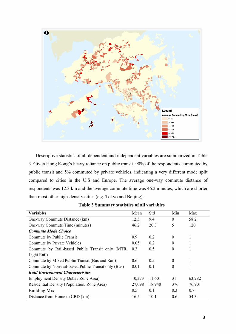
Descriptive statistics of all dependent and independent variables are summarized in Table
3. Given Hong Kong’s heavy reliance on public transit, 90% of the respondents commuted by
public transit and 5% commuted by private vehicles, indicating a very different mode split
compared to cities in the U.S and Europe. The average one-way commute distance of
respondents was 12.3 km and the average commute time was 46.2 minutes, which are shorter
than most other high-density cities (e.g. Tokyo and Beijing).
Table 3 Summary statistics of all variables
Variables Mean Std Min Max One-way Commute Distance (km) 12.3 9.4 0 58.2 One-way Commute Time (minutes) 46.2 20.3 5 120 Commute Mode Choice Commute by Public Transit 0.9 0.2 0 1 Commute by Private Vehicles 0.05 0.2 0 1 Commute by Rail-based Public Transit only (MTR, Light Rail)
0.3 0.5 0 1
Commute by Mixed Public Transit (Bus and Rail) 0.6 0.5 0 1 Commute by Non-rail-based Public Transit only (Bus) 0.01 0.1 0 1 Built Environment Characteristics Employment Density (Jobs / Zone Area) 10,373 11,601 31 63,282 Residential Density (Population/ Zone Area) 27,098 18,940 376 76,901 Building Mix 0.5 0.1 0.3 0.7 Distance from Home to CBD (km) 16.5 10.1 0.6 54.3

4
Distance from Workplace to CBD (km) 11.2 9.7 0.1 54.3 Distance from Home to Rail Stations (km) 1.6 1.8 0 21.8 Number of Non-rail Public Transport Routes 14.9 14.6 0 115 Number of Non-rail Public Transport Stops 2.7 3 0 25 Road Density (Road Area / Total Area) 0.1 0.1 0.004 0.4 Ratio of Residential Area within Rail Catchment (Residential Area within Rail Catchment / Total Residential Area)
0.5 0.3 0 1
Ratio of Commercial Area within Rail Catchment (Commercial Area within Rail Catchment / Total Commercial Area)
0.5 0.3 0 1
Demographic & Socioeconomic Characteristics Gender (1=male) 0.6 0.5 0 1 Age 40.4 11.6 15 99 Driver License (1=yes) 0.4 0.5 0 1 Number of Household Members 3.4 1.3 1 11 Household Income (HKD) 33,644 24,146 0 150,000 Number of Private Vehicles in Household 0.2 0.5 0 10

5
4. Research Methodology
4.1 Baseline Model
Multiple linear regression models were used to investigate how commute distance and
commute duration are related to different built environment features. Our baseline model is
the following: log (𝑌𝑖) = 𝛼0 + 𝛼1𝐵𝐸𝐹𝑖 + 𝛼2𝐻𝐶𝑖 + 𝜀𝑑
We used a log-linear specification where we observed as the commute distance or 𝑌𝑖
commute time of respondent i. is a set of variables measuring a range of built 𝐵𝐸𝐹𝑖
environment factors where respondent i lives. This vector incorporates eleven variables
indicating the characteristics of respondent i’s home zone: employment density, residential
density, building mix, distance from respondent i’s home to CBD, distance from respondent
i’s workplace to CBD, distance from respondent i’s home to the nearest rail station(s), the
number of non-rail public transport routes; the number of non-rail public transport stops, road
density of home zone, the ratio of residential area within 500-meter rail catchment in the
home zone, and the ratio of commercial area within 500-meter rail catchment. The
measurements for each of these eleven built environment variables have been explained in
previous section. In addition, is a set of variables measuring the demographic and 𝐻𝐶𝑖
household characteristics of respondent i, including gender, age, possession of a driver
license, number of household members, household income and the number of private
vehicles in the household.
4.2 Addressing heterogeneity bias
The average effects estimated from the above baseline model would mask considerable
heterogeneity in the effects of built environment across different commute modes and
different neighborhood types. We further divided the sample into groups to investigate how
the relationships between commute behavior and built environment varied across commute
modes and neighborhood types. We compared privately owned vehicle (POV) commuters
versus public transit commuters, as well as within the three public transit sub-modes (rail-
based, non-rail-based, and mixed). We also compared across four different neighborhood
types (i.e. job-dense downtown, urban, new town, rural areas).
4.2.1 Heterogeneity across different commute modes
Commute mode is an important factor that should be considered while estimating the
effects of built environment on commuting behavior. Commute modes can be divided into

6
Privately Owned vehicle (POV) and public transit. According to the statistics of the 2016
Population By-Census10, around 80% working population with a fixed place of work in Hong
Kong were commuting by public transit, among which the largest proportion were using
mass transit railway, accounting for 42.5% of the total work population. Given the significant
portion of public transit commuters in Hong Kong, it is important to investigate the different
sub-modes within the public transport category, in addition to the traditional comparison
between car users and transit users. Therefore, we further divided public transit commute
mode into three sub-modes, as classified in Table 4.
Table 4 The classification and explanation of commute modes
Commute mode Explanation
Privately Owned Vehicles
(POV)
All the trip legs were made by private vehicles
Rail-based
public transport
Public transport trips with all trip legs made by MTR, Airport
Express or Light Rail (LRT)
Non-rail-based
public transport
Public transport trips without any trip legs made by rail-based
transport and could include other road-based or water-based
public transport, e.g. tram, franchised bus, public light bus,
ferry.
Public
transport
modes
Mixed public
transport
Combination of rail-based and non-rail-based public transport,
usually with non-rail-based public transport trip leg for the first
or last mile of commuting trips
The classification of commute modes was based on the primary data obtained from the
Travel Characteristics Survey 2011 (TCS 2011)11, provided by the Transport Department,
Hong Kong SAR. According to TSC 2011, around 6% of the total commuting trips were
made by private vehicles, with the rest made by public transportation. Note that the TCS2011
database includes records of non-motorized modes such as biking and walking, which
account for only a very small percentage of commuting trips in Hong Kong. Only 0.67% of
people commuted on foot and 0.43% by bike, which was possibly due to topological
10 “2016 Population By-Census," Population Census, accessed July 26, 2018, https://www.bycensus2016.gov.hk/en/bc-mt.html 11 "Travel Characteristics Survey 2011 Final Report," Transport Department, February 2014, , accessed July 26, 2018, http://www.td.gov.hk/filemanager/en/content_4652/tcs2011_eng.pdf.

7
inconvenience.12 Hence, all analyses in this paper excluded workers commuted by non-
motorized modes.
4.2.2 Heterogeneity across different neighborhood types
In addition, the relationships between built environment and commuting patterns may
also vary across different neighborhood types. Four neighborhood types were examined in
this study as they represent various unique urban/rural settings in the context of Hong Kong,
including Job-Dense Downtown Areas, Non-downtown Urban Areas, New Town Areas and
Rural Areas. Job-dense downtown areas (e.g. Central, Tsim Sha Tsui) refer to the central
business district (CBD) and its surrounding areas, characterized by intensive economic
activities and employment opportunities. It has the highest connectivity and is also the
destination people often commute to. Non-downtown urban areas (e.g. Wong Tai Sin, Sham
Shui Po) are densely populated and closely connected neighborhoods that are not too far from
the CBD. The New Town Development (e.g. Sha Tin) program was initiated in 1973 and
aimed to develop well-planned neighborhoods in rural areas. New town areas were built with
a balanced combination of residential, commercial, social, public and transport land use,
using heavy rail to connect to city center. It is reported that over half of Hong Kong’s
population were living in New Towns as of 2016 (Civil Engineering and Development
Department, 2016). Rural areas (e.g. Kwu Tung) are sparsely populated, with low density and
few economic activities. As such, they have relatively poor connectivity and are often used
for agricultural purposes. Nonetheless, rural areas are considered potential sites for New
Development Area in the “Hong Kong 2030+” plan, e.g. Kwu Tung. Figure 3 shows the
spatial distribution of these four types of neighborhoods across Hong Kong. Correspondingly,
Figure 4 illustrates the spatial distribution of two selected built environment features--
residential density and employment density, in order to provide some additional insight into
the differences across these four neighborhood types.
12 To be classified as commuting by non-mechanized modes, the respondent has to be walking or biking for the entire commuting trip, a.k.a., using walk or bike for all trip legs of a commuting trip.

8
Figure 2 – Spatial distribution of different types of neighborhoods in Hong Kong
Figure 3 – Spatial distribution of residential density
Figure 4 – Spatial distribution of employment density

9
5. Results
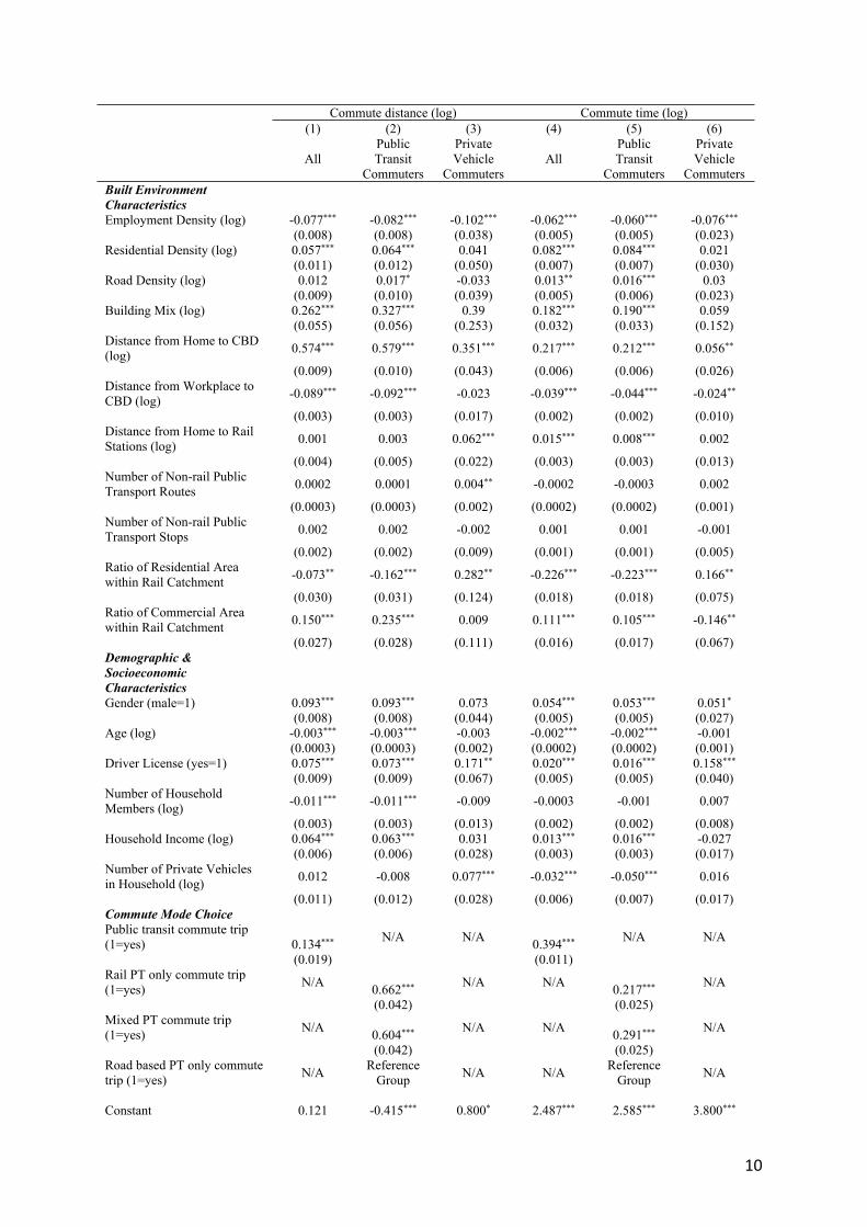
5.1 Commute Distance and Duration for Car Users and Transit Users Table 2 reports our estimates for the effects of various built environment and household
characteristics attributes on commute distance and commute time. In general, as shown in
models (1) and (4), seven built environment features have statistically significant effects on
both commute distance and commute duration. Employment density, distance from
workplace to CBD, and ratio of residential area within 500-meter rail catchment are
negatively correlated with commute distance and time, while residential density, building mix,
distance from home to CBD, and ratio of commercial area within 500-meter rail catchment
are positively correlated with commute distance and time.13 Note that a few built
environment features have shown relationships with commute distance and time that are in
contrast with findings in the majority of previous studies. This is because of the non-linear
nature of some of these effects, which will be addressed and discussed through more in-depth
analyses in following sections.
Table 2 Commute Distance and Duration for All Commuters, Private Vehicle Commuters and Public Transit Commuters
13 Note that building mix is different from the traditional measure of land use mix. The building mix index has high values in downtown areas because of the mixture of commercial, office, hotel, and government buildings. High building mix index does not suggest a good match between housing and jobs. It is not to be confused as a job-housing balance measurement.
10
Commute distance (log) Commute time (log) (1) (2) (3) (4) (5) (6)
All Public Transit
Commuters
Private Vehicle
Commuters All
Public Transit
Commuters
Private Vehicle
Commuters Built Environment Characteristics
Employment Density (log) -0.077*** -0.082*** -0.102*** -0.062*** -0.060*** -0.076*** (0.008) (0.008) (0.038) (0.005) (0.005) (0.023) Residential Density (log) 0.057*** 0.064*** 0.041 0.082*** 0.084*** 0.021 (0.011) (0.012) (0.050) (0.007) (0.007) (0.030) Road Density (log) 0.012 0.017* -0.033 0.013** 0.016*** 0.03 (0.009) (0.010) (0.039) (0.005) (0.006) (0.023) Building Mix (log) 0.262*** 0.327*** 0.39 0.182*** 0.190*** 0.059 (0.055) (0.056) (0.253) (0.032) (0.033) (0.152) Distance from Home to CBD (log) 0.574*** 0.579*** 0.351*** 0.217*** 0.212*** 0.056** (0.009) (0.010) (0.043) (0.006) (0.006) (0.026) Distance from Workplace to CBD (log) -0.089*** -0.092*** -0.023 -0.039*** -0.044*** -0.024** (0.003) (0.003) (0.017) (0.002) (0.002) (0.010) Distance from Home to Rail Stations (log) 0.001 0.003 0.062*** 0.015*** 0.008*** 0.002 (0.004) (0.005) (0.022) (0.003) (0.003) (0.013) Number of Non-rail Public Transport Routes 0.0002 0.0001 0.004** -0.0002 -0.0003 0.002 (0.0003) (0.0003) (0.002) (0.0002) (0.0002) (0.001) Number of Non-rail Public Transport Stops 0.002 0.002 -0.002 0.001 0.001 -0.001 (0.002) (0.002) (0.009) (0.001) (0.001) (0.005) Ratio of Residential Area within Rail Catchment -0.073** -0.162*** 0.282** -0.226*** -0.223*** 0.166** (0.030) (0.031) (0.124) (0.018) (0.018) (0.075) Ratio of Commercial Area within Rail Catchment 0.150*** 0.235*** 0.009 0.111*** 0.105*** -0.146** (0.027) (0.028) (0.111) (0.016) (0.017) (0.067) Demographic & Socioeconomic Characteristics
Gender (male=1) 0.093*** 0.093*** 0.073 0.054*** 0.053*** 0.051* (0.008) (0.008) (0.044) (0.005) (0.005) (0.027) Age (log) -0.003*** -0.003*** -0.003 -0.002*** -0.002*** -0.001 (0.0003) (0.0003) (0.002) (0.0002) (0.0002) (0.001) Driver License (yes=1) 0.075*** 0.073*** 0.171** 0.020*** 0.016*** 0.158*** (0.009) (0.009) (0.067) (0.005) (0.005) (0.040) Number of Household Members (log) -0.011*** -0.011*** -0.009 -0.0003 -0.001 0.007 (0.003) (0.003) (0.013) (0.002) (0.002) (0.008) Household Income (log) 0.064*** 0.063*** 0.031 0.013*** 0.016*** -0.027 (0.006) (0.006) (0.028) (0.003) (0.003) (0.017) Number of Private Vehicles in Household (log) 0.012 -0.008 0.077*** -0.032*** -0.050*** 0.016 (0.011) (0.012) (0.028) (0.006) (0.007) (0.017) Commute Mode Choice Public transit commute trip (1=yes) 0.134*** N/A N/A 0.394*** N/A N/A
(0.019) (0.011) Rail PT only commute trip (1=yes) N/A 0.662*** N/A N/A 0.217*** N/A
(0.042) (0.025) Mixed PT commute trip (1=yes) N/A 0.604*** N/A N/A 0.291*** N/A
(0.042) (0.025) Road based PT only commute trip (1=yes) N/A Reference
Group N/A N/A Reference Group N/A
Constant 0.121 -0.415*** 0.800* 2.487*** 2.585*** 3.800***

11
(0.117) (0.125) (0.467) (0.069) (0.074) (0.282) Number of Observations 33,741 31,678 2,063 33,741 31,678 2,063 Adjusted R2 0.262 0.271 0.243 0.162 0.136 0.119 Notes *p<0.1; **p<0.05; ***p<0.01
Among these seven built environment variables, distance from home to CBD has the
largest impact. A 1% increase in home to CBD distance would lead to an increase in
commute distance by 0.57% and an increase in commute time by 0.22% for an average
commuter. This might be because a large portion of job opportunities still concentrating in
and around CBD in Hong Kong. In addition, a 1% increase in employment density at the
TPUSB where the worker resides would on average contribute to a decrease in commute
distance by 0.08% and commute time by 0.06%. This result corroborates the importance of
job-housing balance at the local level in reducing commute distance and time.
It is important to note that the average treatment effects as shown in models (1) and (4)
disguise the heterogeneity between public transit commuters and private vehicle commuters.
For example, it is observed that, overall, the ratio of residential area within 500-meter rail
catchment is negatively correlated with commute distance and time. But when we divide the
sample into public transit commuters and private car commuters, the coefficient estimates
indicate that a higher ratio of residential area within 500-meter rail catchment reduces the
commute distance and time for public transit commuters (as shown in models 2 and 5), while
it increases the commute for private vehicle commuters (as shown in models 3 and 6). This is
because residents who live in the TPUSBs with higher coverage of rail transit services can
reach transit stations more easily, but for private vehicle commuters, higher coverage of rail
transit typically means higher density and more congested streets.
Heterogeneity between public transit commuters and private vehicle commuters could
also be observed in the effects of other built environment attributes, as shown in Table 5. In
general, we found that public transit commuters are more responsive to built environment
characteristics than private vehicle commuters. For instance, a 1% increase in the distance
from home to CBD would increase commute distance by 0.58% and commute time by 0.21%
for public transit commuters, but the effects for private vehicle commuters are only 0.35%
and 0.06%, respectively. These different elasticities may be ascribed to the different
properties of these two commute modes. Public transit is a less flexible travel mode than
private vehicle in the sense that public transit usually has fixed and indirect routes while
private vehicles can choose among many. Compared to public transit, commuting by private

12
vehicles could be more adaptive with the change of destination accessibility, and hence have
lower elasticities.
5.2 Commute distance and duration for Sub-modes of Public Transit
Given that public transportation plays a critical role in Hong Kong’s transportation
network, it is important to look at the various sub-modes of public transit. Table 3 reports the
estimated effects of built environment features on commute distance and time for rail-based,
mixed-mode, and non-rail-based public transit commuters.
Table 3 Commute Distance and Duration for Sub-modes of Public Transit Commute distance (log) Commute time (log) (1) (2) (3) (4) (5) (6)
Rail PT only commute
trip
Mixed PT commute
trip
Non-rail-based PT
only commute
trip
Rail PT only commute
trip
Mixed PT commute
trip
Non-rail-based PT
only commute
trip Built Environment Characteristics
Employment Density (log) -0.058*** -0.071*** -0.814** -0.034*** -0.059*** -0.335 (0.013) (0.011) (0.346) (0.008) (0.006) (0.249) Residential Density (log) 0.002 0.037** 0.785 0.059*** 0.070*** 0.422 (0.022) (0.015) (0.566) (0.014) (0.009) (0.408) Road Density (log) -0.009 0.030** 0.02 -0.034*** 0.030*** 0.122** (0.016) (0.012) (0.074) (0.010) (0.007) (0.053) Building Mix (log) 0.519*** 0.116 0.205 0.299*** 0.102** -0.217 (0.095) (0.073) (2.841) (0.060) (0.042) (2.045) Distance from Home to CBD (log) 0.564*** 0.560*** 0.490*** 0.210*** 0.200*** 0.247*** (0.015) (0.013) (0.117) (0.010) (0.007) (0.085) Distance from Workplace to CBD (log)
-0.059*** -0.110*** -0.088** -0.021*** -0.059*** -0.018
(0.005) (0.005) (0.036) (0.003) (0.003) (0.026) Distance from Home to Rail Stations (log) 0.014*** 0.0003 -0.055 0.018*** 0.004 -0.057 (0.005) (0.007) (0.052) (0.003) (0.004) (0.038) Number of Non-rail Public Transport Routes -0.002*** 0.002*** -0.004* -0.001*** 0.001* -0.002 (0.001) (0.001) (0.003) (0.0003) (0.0003) (0.002) Number of Non-rail Public Transport Stops 0.011*** -0.005** 0.022 0.001 -0.002 0.015 (0.003) (0.002) (0.029) (0.002) (0.001) (0.021) Ratio of Residential Area within Rail Catchment
-0.179*** -0.029 -1.889** -0.310*** -0.134*** -1.163*
(0.049) (0.043) (0.933) (0.031) (0.025) (0.671) Ratio of Commercial Area within Rail Catchment
0.076 0.168*** 0.428 0.087*** 0.053** -0.187
(0.051) (0.036) (0.930) (0.032) (0.021) (0.669) Demographic & Socioeconomic Characteristics
Gender (male=1) 0.048*** 0.117*** 0.009 0.017** 0.070*** 0.079* (0.012) (0.011) (0.063) (0.008) (0.006) (0.045)

13
Age (log) -0.002*** -0.004*** -0.0004 -0.001*** -0.002*** -0.0005 (0.001) (0.0005) (0.003) (0.0003) (0.0003) (0.002) Driver License (yes=1) 0.047*** 0.081*** -0.119 0.017* 0.015** -0.07 (0.014) (0.012) (0.081) (0.009) (0.007) (0.058) Number of Household Members (log) -0.002 -0.017*** -0.035 0.002 -0.004 -0.008 (0.004) (0.004) (0.023) (0.003) (0.002) (0.016) Household Income (log) 0.035*** 0.083*** 0.053 0.013*** 0.019*** 0.022 (0.007) (0.008) (0.040) (0.005) (0.004) (0.028) Number of Private Vehicles in Household (log)
0.014 -0.014 -0.156 -0.003 -0.060*** -0.087
(0.020) (0.014) (0.169) (0.012) (0.008) (0.122) Constant 0.856*** 0.389** 0.41 2.739*** 3.099*** 2.706
(0.224) (0.157) (4.322) (0.142) (0.090) (3.111) Number of Observations 9,665 21,701 312 9,665 21,701 312 Adjusted R2 0.335 0.235 0.419 0.159 0.107 0.171 Notes *p<0.1; **p<0.05; ***p<0.01
As shown in Table 6, among the various built environment characteristics, distance from
home to CBD is the only factor that significantly affects both commute distance and time for
all sub-modes of public transit. A 1% increase in the home to CBD distance would contribute
to an increase in commute distance by 0.56%, 0.56% and 0.49%, as well as an increase in
commute time by 0.21%, 0.20%, and 0.25% for rail-based commuters, mixed-mode
commuters and non-rail-based commuters, respectively. Moreover, we also noticed that most
built environment attributes have stronger effects on commute distance than on commute
time, based on the sizes of the coefficient estimates. That is, the elasticities of commute time
with respect to various built environment features are smaller than the elasticities of commute
distance. This could be explained by the fast speed of the highly reliable public transit system,
especially the railway network, in Hong Kong, which helps public transit commuters to travel
efficiently.
It is worth noting that a higher ratio of residential area within 500-meter rail catchment
reduces commuting distance and time, hence improves job accessibility for both rail-based
and non-rail-based public transit commuters. With a 1 percentage point increase in the ratio
of residential area within rail catchment, commute distance would reduce by 0.18% for rail-
based commuters and by 1.89% for non-rail-based commuters, while commute time would
reduce by 0.31% for rail-based commuters and by 1.16% for non-rail-based commuters. This
suggests that, to improve job accessibility, current urban planning and policies on transit-
oriented development should consider planning residential units around transit nodes to
enhance the connectivity and workability of public transit commuters.

14
Our results also reveal other heterogeneous effects across different public transit sub-
modes. Employment density is negatively correlated with commute distance for all public
transit commuters as the point estimates have the same sign. But the effect is most significant
(in terms of magnitude) for non-rail-based public transit commuters, while the effects for rail-
based and mixed-mode commuters are marginal. If employment density at home zone
increases by 1%, the commute distance would drop by 0.81% for non-rail-based commuters
but only by 0.06% for rail-based commuters. This result could be because non-rail-based
commuters are mostly working in districts not far away from their home zone, therefore,
increasing employment density could significantly reduce their commute distance.
5.3 Commute Distance and Duration for Commuters in Different Neighborhoods
In this section, we further break down the groups into Public Transit Commuters and
Private Vehicle Commuters living in four different neighborhoods, as discussed earlier.
5.3.1 Commute distance and duration for Public Transit Commuters by Different
Neighborhoods
The model results for public transit commuters by different neighborhoods are summarized
in Table 4. Distance from home to CBD is positively correlated to commute distance in all
four types of neighborhoods. This effect is found most significant for rural public transit
commuters. A 1% increase in distance from home to CBD would contribute to a 0.41%,
0.51%, 0.85% and 1.03% increase on commute distance in job-dense downtown areas, non-
downtown urban areas, new towns areas and rural areas, respectively. This suggests that a lot
of people are still relying on the CBD for work even if they live far from the area.
The distance from workplace to CBD also shows significant effects on the commute
distance of public transit commuters in job-dense downtown, urban, new town and rural
neighborhoods, with elasticities of 0.109, 0.048, -0.261 and -0.375, respectively. In the
meantime, a 1% increase in distance from workplace to CBD would increase commute
duration by 0.07% in job-dense downtown neighborhoods, but reduce it by 0.13% in new
town neighborhoods and 0.18% in rural neighborhoods. Job-dense downtown areas are the
closest to CBD, followed by non-downtown urban areas, new town areas and rural areas.
These results suggest that public transit commuters who are living and working in new town
areas or rural areas are better off in terms of job accessibility, compared with those living in
urban areas but working closer to CBD. Clearly, job decentralization in the event of CBD
being already over-crowded may be beneficial, especially to those living out of the urban
cores.

15
Table 4 Commute distance and duration for public transit commuters in different
neighborhoods Commute distance (log) Commute time (log) (1) (2) (3) (4) (5) (6) (7) (8)
Job-
dense downtow
n
Non-downtown Urban
New Town Rural
Job-dense
downtown
Non-downtown Urban
New Town Rural
Built Environment Characteristics
Employment Density (log) 2.208*** -1.057*** -0.086*** -0.11 0.262 0.142 -0.067*** 0.043 (0.397) (0.302) (0.021) (0.173) (0.233) (0.186) (0.012) (0.106) Residential Density (log) 2.114*** -1.398*** 0.042* -0.328** 0.409* 0.377 0.091*** 0.162* (0.384) (0.495) (0.022) (0.154) (0.225) (0.305) (0.013) (0.094) Road Density (log) -0.054*** -0.002 0.053*** 0.074** -0.009 -0.006 0.01 0.052** (0.017) (0.026) (0.016) (0.035) (0.010) (0.016) (0.010) (0.021) Building Mix (log) 12.098*** -0.078 -0.118 1.58 1.469 0.125 0.162** -1.637**
(1.974) (0.388) (0.116) (1.299) (1.157) (0.238) (0.069) (0.798) Distance from Home to CBD (log) 0.409*** 0.506*** 0.847*** 1.029*** 0.086*** 0.058 0.294*** 0.075 (0.030) (0.069) (0.020) (0.119) (0.018) (0.042) (0.012) (0.073) Distance from Workplace to CBD (log) 0.109*** 0.048*** -0.261*** -0.375*** 0.066*** 0.004 -0.130*** -0.181*** (0.006) (0.007) (0.005) (0.016) (0.004) (0.004) (0.003) (0.010) Distance from Home to Rail Stations (log) 0.013* 0.021 0.002 0.018 0.011** 0.066*** 0.005 -0.013 (0.008) (0.020) (0.006) (0.029) (0.005) (0.012) (0.004) (0.018) Number of Non-rail Public Transport Routes -0.00001 -0.001 0.0004 -0.007 0.00004 -0.001* 0.0001 0.001 (0.001) (0.001) (0.001) (0.008) (0.0003) (0.0003) (0.0004) (0.005) Number of Non-rail Public Transport Stops -0.002 0.008** 0.001 0.013 -0.003 0.003 -0.002 -0.0005 (0.004) (0.003) (0.003) (0.013) (0.002) (0.002) (0.002) (0.008) Ratio of Residential Area within Rail Catchment
-2.076*** -13.221*
** -0.111* -0.420** 2.632 -0.332***
(0.365) (4.417) (0.062) (0.214) (2.718) (0.037) Ratio of Commercial Area within Rail Catchment
20.586*** 0.008 -4.224 0.144***
(6.777) (0.045) (4.170) (0.027) Demographic & Socioeconomic Characteristics
Gender (male=1) 0.065*** 0.123*** 0.089*** 0.015 0.045*** 0.066*** 0.050*** 0.005 (0.016) (0.016) (0.012) (0.039) (0.009) (0.010) (0.007) (0.024) Age (log) -0.001* -0.003*** -0.004*** -0.005*** -0.001** -0.001*** -0.002*** -0.004*** (0.001) (0.001) (0.001) (0.002) (0.0004) (0.0004) (0.0003) (0.001) Driver License (yes=1) 0.051*** 0.071*** 0.066*** 0.120*** 0.001 0.004 0.019** 0.065** (0.017) (0.018) (0.013) (0.042) (0.010) (0.011) (0.008) (0.026) Number of Household Members (log) 0.0002 -0.020*** -0.013*** -0.029* 0.008** -0.010** -0.003 0.002 (0.006) (0.006) (0.005) (0.015) (0.003) (0.004) (0.003) (0.009) Household Income (log) 0.034*** 0.068*** 0.064*** 0.174*** 0.011** 0.025*** 0.012** -0.0004 (0.008) (0.012) (0.009) (0.040) (0.005) (0.007) (0.006) (0.024) Number of Private Vehicles in Household (log)
-0.032 0.024 -0.023 0.039 -0.069*** -0.042*** -0.047*** -0.009
(0.023) (0.025) (0.017) (0.034) (0.013) (0.015) (0.010) (0.021) Commute Mode Choice Rail PT only commute trip (1=yes) 0.777*** -0.356 -0.24 -0.287 0.221*** -0.367 -0.172 -0.179 (0.042) (0.680) (0.204) (0.468) (0.025) (0.418) (0.122) (0.288) Mixed PT commute trip 0.708*** -0.504 -0.277 -0.629 0.265*** -0.327 -0.072 -0.166

16
(1=yes) (0.041) (0.680) (0.204) (0.458) (0.024) (0.418) (0.122) (0.281) Non-rail-based PT only commute trip (1=yes)
Reference Group
Reference Group
Reference Group
Reference Group
Reference Group
Reference Group
Reference Group
Reference Group
Constant -49.733*** 20.300*** 0.712** 0.919 -4.467 -0.689 2.974*** 4.240*** (8.837) (6.448) (0.305) (0.782) (5.179) (3.968) (0.183) (0.480) Number of Observations 7,996 7,891 14,591 1,200 7,996 7,891 14,591 1,200 Adjusted R2 0.193 0.066 0.268 0.419 0.137 0.056 0.158 0.257 Notes *p<0.1; **p<0.05; ***p<0.01
Our results indicate that higher employment density reduces commute distance for transit
commuters living in non-downtown urban neighborhoods and new town neighborhoods, as
many literatures would suggest. However, we did find that it increases commute distance,
hence reduces job accessibility for those living in job-dense downtown neighborhoods. With
a 1% increase in employment density in their home zone, public transit commuter’s commute
distance would be reduced by 1.06% in non-downtown urban areas and by 0.09% in new
town areas, whereas it would be increased by 2.21% in job-dense downtown areas. Note that
the employment density in job-dense downtown areas of Hong Kong is already very high.
Further intensifying employment density in these areas may exert a crowding out effect on
people living in these neighborhoods, as additional offices or commercial uses outbid existing
residential uses, which may actually increase their commute distance and time. Additionally,
as downtown areas become over-crowded, agglomeration diseconomies such as congestion,
noise, crime may drive people to move out of these neighborhoods voluntarily. On the
contrary, as shown in columns (2) and (3), increasing employment density in non-downtown
urban areas and new town areas reduces commute distance for transit commuters living in
these neighborhoods, which implies that job provisions in these areas may effectively
improve job accessibilities for their residents. Interestingly, the elasticity is around -1,
suggesting 1% increase in employment density in these areas is associated with a 1%
reduction in commute distance. In sum, our results elaborate that the impact of employment
density on commute distance/time and job accessibility is not linear. Many previous studies
overlooked this important non-linear relationship, possibly because their study areas might
not have reached an employment density comparable to that in downtown Hong Kong and
such non-linearity was not detected in their data analyses.
Residential density also shows opposite effects on commute distance in job-dense
downtown neighborhoods versus that in non-downtown urban neighborhoods. Job-dense
downtown neighborhoods with higher residential density is associated with longer average
commute distance, with an elasticity of 2.11 (for transit commuters). Classic urban land bid

17
rent theory clearly plays a role here. Neighborhoods with higher residential density in job-
dense downtown areas are usually located not directly at the downtown core, but at a small
distance from it, because the land rent residential usage can afford is lower than the land rent
bid by commercial and office uses. In case of an extremely dense downtown area like the one
in Hong Kong, the most valuable land has been occupied by transnational corporation
(regional) headquarters, luxury hotel chains, fancy restaurants, and high-end shopping malls.
Within the boundary of job-dense downtown area, neighborhoods with relatively higher
residential density are located at the edge (between job-dense downtown area and non-
downtown urban areas), which explains why their residents have relatively longer commute
distance as they travel to downtown core to work. On the contrary, non-downtown urban
neighborhoods would have shorter average commute distance if their residential density is
higher, with an elasticity of -1.40 (for transit commuters). In general, non-downtown urban
neighborhoods with higher residential density are located at (or close to) urban sub-centers,
where residential use often coexists with commercial and office uses. This can be attributed
to Hong Kong government’s continuous efforts since the 1980s to develop strategic plans and
effective implementations for mixed land use in the city’s new centers, as well as its
emphasis on transit-oriented development in recent years. As a result, non-downtown urban
areas with higher residential density usually also have higher overall density and contain
plenty of commercial and office spaces.
Note that the ratio of residential areas and the ratio of commercial areas within 500-meter
rail catchment affect commute distance much more significantly (in terms of magnitude) in
non-downtown urban areas than in job-dense downtown areas or new town areas. Table 7
column (2) reports that a 1 percentage point increase in the ratio of residential areas within
rail catchment would reduce commute distance by 13.2%, while a 1 percentage point increase
in the ratio of commercial areas within rail catchment would increase commute distance by
20.6%. These results corroborate the importance of mixed land use and TOD, especially in
non-downtown urban areas. Increasing the share of residential use within 500 meters from
rail stations would lead to better job accessibility for an average transit commuter. However,
at its current density, further increasing the share of commercial uses within 500 meters from
rail stations could increase commute distance and impair job accessibility for the majority of
transit commuters living in these urban areas. This is because of the same crowding out effect
as we observed in job-dense downtown areas. Residents will be forced to live further away
from these rail stations if commercial uses take up more land near the stations. In summary,

18
planners need to be cautious about a well-balanced land use mix between residential and
commercial uses when implementing TOD.
5.3.2 Commute distance and duration for Private Vehicle Commuters by Different
Neighborhoods
The model results for private vehicle commuters by different neighborhoods are
presented in Table 5. The results are consistent with those of public transit commuters.
Among these built environment characteristics, distance from home to CBD and distance
from workplace to CBD show the most significant effects on commute distance/time for
private vehicle commuters in all four types of neighborhoods. Similar to what we observed
on public transit commuters, longer workplace to CBD distance would reduce commute
distance and time and hence improve job accessibility for private vehicle commuters living in
new town areas and rural areas. The magnitudes of these effects are similar to those on public
transit commuters. In addition, the non-linearity in the impact of employment density on
commute distance/time across different neighborhood types is also observed for private
vehicle commuters. In summary, job decentralization to new development areas in a highly
dense urban context such as Hong Kong is beneficial.
Table 5 Commute Distance and Duration for Private Vehicle Commuters in Different Neighborhoods Commute distance (log) Commute time (log) (1) (2) (3) (4) (5) (6) (7) (8)
Job-dense
downtown
Urban New Town Rural
Job-dense
downtown
Urban New Town Rural
Built Environment Characteristics
Employment Density (log) 2.429*** -1.110*** -0.092*** -0.023 0.467** 0.310* -0.056*** 0.145 (0.388) (0.291) (0.021) (0.164) (0.232) (0.181) (0.013) (0.103) Residential Density (log) 2.322*** -1.524*** 0.044** -0.293** 0.608*** 0.676** 0.065*** 0.105 (0.373) (0.479) (0.022) (0.138) (0.223) (0.299) (0.013) (0.087) Road Density (log) -0.066*** 0.004 0.058*** 0.065** -0.017* -0.002 0.027*** 0.037* (0.017) (0.026) (0.016) (0.031) (0.010) (0.016) (0.010) (0.020) Building Mix (log) 12.950*** -0.266 -0.132 1.079 2.435** 0.257 0.039 -1.893** (1.930) (0.386) (0.114) (1.199) (1.153) (0.241) (0.070) (0.754) Distance from Home to CBD (log) 0.446*** 0.499*** 0.821*** 1.018*** 0.106*** 0.021 0.305*** 0.051 (0.029) (0.066) (0.019) (0.109) (0.017) (0.041) (0.012) (0.069) Distance from Workplace to CBD (log)
0.124*** 0.044*** -0.267*** -0.360*** 0.074*** 0.003 -0.131*** -0.178***
(0.006) (0.007) (0.005) (0.015) (0.004) (0.004) (0.003) (0.009) Distance from Home to Rail Stations (log) 0.004 -0.014 -0.0005 0.022 0.011** 0.083*** 0.010*** -0.023 (0.008) (0.018) (0.006) (0.027) (0.005) (0.011) (0.003) (0.017) Number of Non-rail -0.001 -0.0002 0.001 -0.008 0.0001 -0.0004 0.0002 -0.0004

19
Public Transport Routes (0.001) (0.001) (0.001) (0.007) (0.0004) (0.0003) (0.0004) (0.005) Number of Non-rail Public Transport Stops
-0.001 0.007** 0.001 0.008 -0.002 0.004** -0.003* -0.002
(0.004) (0.003) (0.003) (0.012) (0.002) (0.002) (0.002) (0.008) Ratio of Residential Area within Rail Catchment
-2.186*** -13.970**
* -0.099 -0.598*** 5.214** -0.347***
(0.356) (4.260) (0.060) (0.213) (2.654) (0.037) Ratio of Commercial Area within Rail Catchment
21.807*** -0.003 -8.177** 0.183***
(6.536) (0.043) (4.071) (0.026) Demographic & Socioeconomic Characteristics
Gender (male=1) 0.071*** 0.114*** 0.088*** 0.007 0.043*** 0.052*** 0.037*** -0.038* (0.015) (0.016) (0.012) (0.036) (0.009) (0.010) (0.007) (0.023) Age (log) -0.002*** -0.003*** -0.003*** -0.006*** -0.001*** -0.002*** -0.002*** -0.004*** (0.001) (0.001) (0.001) (0.002) (0.0004) (0.0004) (0.0003) (0.001) Driver License (yes=1) 0.056*** 0.064*** 0.060*** 0.115*** -0.012 -0.006 0.004 0.012 (0.017) (0.018) (0.013) (0.040) (0.010) (0.011) (0.008) (0.025) Number of Household Members (log) 0.003 -0.018*** -0.014*** -0.032** 0.013*** -0.005 -0.001 0.007 (0.006) (0.006) (0.005) (0.014) (0.003) (0.004) (0.003) (0.009) Household Income (log) 0.039*** 0.063*** 0.058*** 0.172*** 0.005 0.015** 0.005 -0.01 (0.008) (0.012) (0.009) (0.035) (0.005) (0.007) (0.006) (0.022) Number of Private Vehicles in Household (log)
-0.002 -0.005 -0.037** 0.034 -0.101*** -0.111*** -0.127*** -0.062***
(0.019) (0.020) (0.014) (0.027) (0.011) (0.013) (0.009) (0.017) Constant -53.944*** 21.565*** 0.646*** 0.035 -8.789* -4.709 3.162*** 4.330*** (8.615) (6.201) (0.226) (0.558) (5.146) (3.863) (0.138) (0.351) Number of Observations 8,481 8,369 15,389 1,502 8,481 8,369 15,389 1,502 Adjusted R2 0.172 0.059 0.259 0.386 0.139 0.058 0.158 0.236 Notes *p<0.1; **p<0.05; ***p<0.01
6. Conclusion
Given the inherent limitations and challenges Hong Kong faces due to scarce land supply,
there have been far from sufficient research applicable to the city’s unique context to support
effective policymaking. Our study for Hong Kong, as an example of cities with high-density,
disentangled the unique features of built environment in a rail-based dense urban setting and
its impacts on people’s commuting behavior and the associated job accessibility. More
importantly, given the high proportion of public transit to Hong Kong’s transportation system
and the heterogeneous features in different neighborhoods, we draw a special focus on how
commute distance and time vary across different commute modes, sub-modes of public
transport, and neighborhood types. By understanding the relationships between urban settings
and travel behavior, one important implication is that infrastructure planning should pay

20
attention to built environments, as these features could significantly impact people’s day-to-
day commute, job accessibility, and ultimately their quality of life.
Uncovering the heterogeneity behind the average effects, we found that public transit
commuters are more responsive to changes of built environments than private vehicle
commuters. Interestingly, we found non-linearity in the impacts of employment density on
people’s commuting distance/time and the associated job accessibility. Our findings provide
cautions about a common argument suggested in many literatures, that higher employment
density would reduce commute distance/time and improve job accessibility. This is not
always the case. In non-downtown urban areas and new town areas, the findings conform to
our conventional wisdom; however, in Hong Kong’s job-dense downtown areas, further
increasing employment density generates negative crowding out effects as residential use gets
outbid by commercial uses and workers are forced to live further away from jobs in
downtown. For Hong Kong and other similar high-density cities, future urban planning
should avoid further densifying employment in CBDs, but to focus more on developing
employment sub-centers so that a more balanced employment distribution can be achieved.
By dispersing residents’ daily peak-hour destinations into multiple centers of the city,
wasteful commuting can be alleviated. This can reduce the commute distance and time for the
majority of the commuters, ease congestions and reduce energy consumption, which
ultimately contribute to people’s wellbeing and overall productivity of the society. For the
whole city, this would be a pareto efficient outcome.
Raising the ratio of residential area within a 500-meter rail catchment can reduce commute
distance/time and improve job accessibility for all modes of public transport commuters as
well as private vehicle commuters. This effect is much stronger in non-downtown urban areas
as opposed to job-dense downtown areas or rural areas. Lowering the share of commercial
uses within a 500-meter rail catchment would have the same effect for non-downtown urban
areas. These results lead to important policy recommendations. For high-density cities like
Hong Kong, transit-oriented development policies which use railway as the backbone of the
public transportation system are commendable. But planners should be careful not to further
increase the share of commercial uses around these rail stations as they will crowd out
residential use and hence impair job accessibility. With the current land use composition,
planners may consider increasing the share of residential use near rail stations in non-
downtown areas in their implementation of TOD. Large scale high-density residential estates
on top or surrounding rail stations may be a good option to optimize connectivity to rail
transit and improves job accessibility for public transit commuters.

21
It is worth noting that the relationship between the built environment and commuting
behavior, as well as our policy recommendations in this paper are all context specific. Our
findings may be applicable to other high-density cities such as Tokyo, Beijing, Shanghai and
Seoul. But we need to be careful when making inferences to relatively low-density urban
contexts. Additionally, our measure of job accessibility using commute distance/time may not
be applicable to cities in North America or Europe because of their relatively lower density.
But for dense urban settings such as Hong Kong, our measure is more appropriate than the
traditional job accessibility measures. Researchers and policymakers need to be cautious
when applying this context-specific job accessibility measure to their own cities. Lastly, we
would like to note that self-selection is not addressed in this study. Although it is not the
objective of this paper to investigate the self-selection problem, the issue could exist. Future
researches could take this into account by supplementing travel diary questionnaires with
attitude surveys, similar to the study conducted by Kitamura et al. (1997).

22
Acknowledgments
Funding: This work was supported by the National Natural Science Foundation of China
[project number: 71573232].
We would also like to acknowledge the contributions made by Ms. Shuk Nuen Ho in her
Master’s Thesis as the preliminary implementation of some of the research ideas presented in
this paper.

23
References
Boisjoly, G., & El-Geneidy, A. M. (2017). How to get there? A critical assessment of accessibility objectives and indicators in metropolitan transportation plans. Transport Policy, 55, 38–50. https://doi.org/10.1016/j.tranpol.2016.12.011
Cao, X. (2009). Disentangling the influence of neighborhood type and self-selection on driving behavior: an application of sample selection model. Transportation, 36(2), 207–222. doi:10.1007/s11116-009-9189-9
Cao, X. J. (2015). Heterogeneous effects of neighborhood type on commute mode choice: an exploration of residential dissonance in the Twin Cities. Journal of transport geography, 48, 188-196.
Cao, X., & Yang, W. (2017). Examining the effects of the built environment and residential self-selection on commuting trips and the related CO2 emissions: An empirical study in Guangzhou, China. Transportation Research Part D, 52(PB), 480-494.
Census and Statistics Department. (2018). Press Release (13 Feb 2018) :Year-end population for 2017 | Census and Statistics Department. Retrieved July 26, 2018, from https://www.censtatd.gov.hk/press_release/pressReleaseDetail.jsp?charsetID=1&pressRID=4213
Cervero, R. (2002). Built environments and mode choice: toward a normative framework. Transportation Research Part D: Transport and Environment, 7(4), 265–284. https://doi.org/10.1016/S1361-9209(01)00024-4
Cervero, R., & Kockelman, K. (1997). Travel demand and the 3Ds: Density, diversity, and design. Transportation Research Part D: Transport and Environment, 2(3), 199–219. https://doi.org/10.1016/S1361-9209(97)00009-6
Cervero, R., & Day, J. (2008) Residential Relocation and Commuting Behavior in Shanghia, China: The Case for Transit Oriented Development. UC Berkeley Center for Future Urban Transport: A Volvo Center of Excellence.
Cheng, J., & Bertolini, L. (2013). Measuring urban job accessibility with distance decay, competition and diversity. Journal of Transport Geography, 30, 100-109.
Civil Engineering and Development Department. (2016). New Towns, New Development Areas and Urban Developments. Retrieved from https://www.gov.hk/en/about/abouthk/factsheets/docs/towns&urban_developments.pdf
Dai, T., Liu, Z., Liao, C., & Cai, H. (2018). Incorporating job diversity preference into measuring job accessibility. Cities, 78, 108-115.
Deboosere, R., & El-Geneidy, A. (2018). Evaluating equity and accessibility to jobs by public transport across Canada. Journal of Transport Geography. https://doi.org/10.1016/j.jtrangeo.2018.10.006
Ding, C., Cao, X., & Wang, Y. (2018). Synergistic effects of the built environment and commuting programs on commute mode choice. Transportation Research Part A, 118, 104-118.
Engelfriet, L., & Koomen, E. (2018). The impact of urban form on commuting in large Chinese cities. Transportation, 45(5), 1269-1295.
Feng, J. (2017). The influence of built environment on travel behavior of the elderly in urban China. Transportation Research Part D, 52(PB), 619-633.
Feng, J., Dijst, M., Prillwitz, J., Wissink, B. (2013). Travel Time and Distance in International Perspective: A Comparison between Nanjing (China) and the Randstad (The Netherlands). Urban Studies, 50(14), 2993-3010.
Geurs, K. T. (2006). Job accessibility impacts of intensive and multiple land-use scenarios for the Netherlands’ Randstad Area. Journal of Housing and the Built Environment, 21(1), 51–67. https://doi.org/10.1007/s10901-005-9032-3
Geurs, K., & Van Wee, B. (2004). Accessibility evaluation of land-use and transport strategies: Review and research directions. Journal of Transport Geography, 12(2), 127-140.
Handy, S., Cao, X., & Mokhtarian, P. (2005). Correlation or causality between the built environment and travel behavior? Evidence from Northern California. Transportation Research Part D, 10(6), 427-444.
Hansen, W. G. (1959). How accessibility shapes land use. Journal of the American Institute of Planners, 25(2), 73-76.
Hess, S., Polak, J. W., Daly, A., & Hyman, G. (2007). Flexible substitution patterns in models of mode and time of day choice: new evidence from the UK and the Netherlands. Transportation, 34(2), 213–238. https://doi.org/10.1007/s11116-006-0011-7

24
Hong, J., Shen, Q., & Zhang, L. (2014). How do built-environment factors affect travel behavior? A spatial analysis at different geographic scales. Transportation, 41(3), 419-440.
Hu, L. (2015). Changing Effects of Job Accessibility on Employment and Commute: A Case Study of Los Angeles. The Professional Geographer, 67(2), 154-165.
Hu, L. (2017). Job accessibility and employment outcomes: Which income groups benefit the most? Transportation, 44(6), 1421-1443.
Hu, L., Sun, T., & Wang, L. (2018). Evolving urban spatial structure and commuting patterns: A case study of Beijing, China. Transportation Research Part D, 59, 11-22.
Hu, L., Yang, J., Yang, T., Tu, Y., & Zhu, J. (2020). Urban Spatial Structure and Travel in China. Journal of Planning Literature, 35(1), 6–24. https://doi.org/10.1177/0885412219853259
Jin, Y., Denman, Deng, Rong, Ma, Wan, . . . Long. (2017). Environmental impacts of transformative land use and transport developments in the Greater Beijing Region: Insights from a new dynamic spatial equilibrium model. Transportation Research Part D, 52(PB), 548-561.
Kim, T., Sohn, D.-W., & Choo, S. (2017). An analysis of the relationship between pedestrian traffic volumes and built environment around metro stations in Seoul. KSCE Journal of Civil Engineering, 21(4), 1443–1452. https://doi.org/10.1007/s12205-016-0915-5
Leung, C. Y. (2017). Make Best Use of Opportunities Develop the Economy Improve People’s Livelihood Build an Inclusive Society. Retrieved from https://policy.asiapacificenergy.org/sites/default/files/PA2017.pdf
Levinson D. M., Kumar A., (1997) Density and the journey to work, Growth and Change, 28(2), pp. 147–172. Lin, D., Allan, A., & Cui, J. (2015). The impact of polycentric urban development on commuting behaviour in
urban China: Evidence from four sub-centres of Beijing. Habitat International, 50, 195-205. Lin, D., Allan, A., & Cui, J. (2016). Exploring Differences in Commuting Behaviour among Various Income Groups
during Polycentric Urban Development in China: New Evidence and Its Implications. Sustainability, 8(11), 1188.
Liu, E., Jackie, M., Mr, W. U., & Lee, J. (1997). Optimization Of Land Use. Retrieved from https://www.legco.gov.hk/yr97-98/english/sec/library/967rp12.pdf
Lu, Y., Sun, G., Sarkar, C., Gou, Z., & Xiao, Y. (2018). Commuting Mode Choice in a High-Density City: Do Land-Use Density and Diversity Matter in Hong Kong? International Journal of Environmental Research and Public Health, 15(5), International Journal of Environmental Research and Public Health, 2018, Vol.15(5).
Ma, L., & Cao, J. (2019). How perceptions mediate the effects of the built environment on travel behavior? Transportation, 46(1), 175–197. https://doi.org/10.1007/s11116-017-9800-4
Maharjan, S., Tsurusaki, N., & Divigalpitiya, P. (2018). Influencing Mechanism Analysis of Urban Form on Travel Energy Consumption-Evidence from Fukuoka City, Japan. https://doi.org/10.3390/urbansci2010015
Marcińczak, S., & Bartosiewicz, B. (2018). Commuting patterns and urban form: Evidence from Poland. Journal of Transport Geography, 70, 31-39.
McKibbin, M. (2011). The influence of the built environment on mode choice – evidence from the journey to work in Sydney. World Transit Research. Retrieved from https://www.worldtransitresearch.info/research/4346
Munshi, T. (2016). Built environment and mode choice relationship for commute travel in the city of Rajkot, India. Transportation Research Part D, 44, 239-253. https://doi.org/10.1016/j.trd.2015.12.005
Næss P., (2005) Residential location affects travel behavior: but how and why? The case of Copenhagen metropolitan area, Progress in Planning, 63(2), pp. 167–257.
Nasri, A., & Zhang, L. (2012). Impact of Metropolitan-Level Built Environment on Travel Behavior. Transportation Research Record: Journal of the Transportation Research Board, 2323(1), 75–79. https://doi.org/10.3141/2323-09
Nasri, A., & Zhang, L. (2018). Multi-level urban form and commuting mode share in rail station areas across the United States; a seemingly unrelated regression approach. Transport Policy. https://doi.org/10.1016/j.tranpol.2018.05.011
Nicholas Ng. (2000). Railways: The Backbone of Hong Kong’s Transport System. Retrieved July 26, 2018, from https://www.info.gov.hk/gia/general/200005/03/0503158.htm
Park, K., Ewing, R., Scheer, B., & Tian, G. (2018). The impacts of built environment characteristics of rail station areas on household travel behavior. Cities, 74, 277-283.
Planning Department. (2016). Planning and Urban Design for a Liveable High-Density City. Retrieved from https://www.hk2030plus.hk/document/Planning and Urban Design for a Liveable High-Density City_Eng.pdf
Planning Department. (2018). Hong Kong 2030+: Towards a Planning Vision and Strategy Transcending 2030. Retrieved from https://www.hk2030plus.hk/document/Conceptual Spatial Framework_Eng.pdf

25
Preliminary Concepts for the New Territories North Development. (2016). Retrieved from https://www.hk2030plus.hk/document/NTN_EN.pdf
Ramsey, K., & Bell, A. (2014). The Smart Location Database: A Nationwide Data Resource Characterizing the Built Environment and Destination Accessibility at the Neighborhood Scale. Cityscape, 16(2), 145-162.
Song, Y., Chen, Y., & Pan, X. (2012). Polycentric spatial structure and travel mode choice: The case of Shenzhen, China. Regional Science Policy & Practice, 4(4), 479-493.
Stead, D., (1999) Relationships between transport emissions and travel patterns in Britain, Transport Policy, 6(4), pp. 247–258.
Sun, B., Ermagun, A., & Dan, B. (2017). Built environmental impacts on commuting mode choice and distance: Evidence from Shanghai. Transportation Research Part D, 52(PB), 441-453.
Ta, N, Y. Chai, Y. Zhang, D. Sun. (2017). Understanding job-housing relationship and commuting pattern in Chinese cities: past, present and future. Transport. Res. Part D: Transp. Environ.
Transport Department. (1999). Transport Department - The Third Comprehensive Transport Study : Final Report *Free copy can only be downloaded from this website. Hong Kong. Retrieved from https://www.td.gov.hk/en/publications_and_press_releases/publications/free_publications/the_third_comprehensive_transport_study/index.html
Transport Infrastructure and Traffic Review Planning Department. (2016). Retrieved from https://www.hk2030plus.hk/document/Transport Infrastructure and Traffic Review_Eng.pdf
Wang D., Chai Y., (2009) The jobs–housing relationship and commuting in Beijing, China: the legacy of Danwei, Journal of Transport Geography, 17(1), pp. 30–38.
Wang, D., & Cao, X. (2017). Impacts of the built environment on activity-travel behavior: Are there differences between public and private housing residents in Hong Kong? Transportation Research Part A, 103, 25-35.
Wang, K. (2013). Causality between Built Environment and Travel Behavior. Transportation Research Record: Journal of the Transportation Research Board, 2397(1), 80–88. https://doi.org/10.3141/2397-10
Wang, Y., Monzon, A., & Ciommo, F. D. (2015). Assessing the accessibility impact of transport policy by a land-use and transport interaction model – The case of Madrid. Computers, Environmnet and Urban Systems, 49, 126-135.
Ye, R., & Titheridge, H. (2017). Satisfaction with the commute: The role of travel mode choice, built environment and attitudes. Transportation Research Part D, 52(PB), 535-547.
Zhang, L., Nasri, A., Hong, J. H., & Shen, Q. (2012). How built environment affects travel behavior: A comparative analysis of the connections between land use and vehicle miles traveled in US cities. Journal of Transport and Land Use, 5(3).
Zhu, Pengyu, Dong, Hongwei, Wu, Cifang, 2013. Do residents of smart growth neighborhoods in Los Angeles travel ‘‘smarter”? Transp. Res. Rec.: J. Transp. Res. Board 2397, 61–71.
Zhu, Pengyu, 2015. Residential segregation and employment outcomes of rural migrant workers in China. Urban Studies. http://dx.doi.org/10.1177/0042098015578614.
Zhu, P., Zhao, S., Wang, L., & Al Yammahi, S. (2017). Residential segregation and commuting patterns of migrant workers in China. Transportation Research Part D, 52(PB), 586-599.

26


