Account o[ the Boundary Layer - Cranfield...

C : ._. :, ~,.2! ': .:, : i

MINISTRY OF SUPPLY

A E R O N A U T I C A L R E S E A R C H C O U N C I L

R E P O R T S A N D M E M O R A N D A

o o o

~he Ca~cu~ac:~on oi ~ L~f'~ takxng Account o[ the Boundary Layer

j. Ho PRBSTON, M.A, Ph.D., AoF.R°Ae.S.,

o f the C a m b r i d g e U n i v e r s i t y A e r o n a u t i c s L a b o r a t o r y

Crown Copyrig/~t Reserved

L O N D O N : HER MAJESTY'S STATIONERY OFFICE

x953

PRICE lOg 6d N E T

,,, ' ' " k

/ ,

The Calculation of.Lift Boundary

taking Layer

Account of the

j . H. PRESTON, M.A., Ph.D., A.F.R.Ae.S. ,

of the Cambridge University Aeronautics Laboratory

Reports and Memoranda No. 2725

2 Ist November, 1949

Summary.--The purpose of this paper is to fred a sound approach to the problem of the theoretical prediction of sectional characteristics taking account of the boundary layer.

Attention is mainly concentrated on the lift, since it is on the accuracy of this calculation that the accuracy of calculations for other characteristics such as pressure distribution and moments must depend. Calculations of the lift and of the velocity at the edge of the boundary layer near tile trailing edge have been made for two dissimilar symmetrical aerofoils at an incidence of 6 deg, using boundary-layer data taken from experiment. Tile method of calculation satisfies the fundamental theorem that no net vorticity is discharged into tile wake at the trailing edge and in contrast to tile earlier calculations of R. & M. 1996, full account is now taken of the effect of the boundary layer on the velocity field outside tile boundary layer, so that tile empiricism of that report is avoided. Tile present- calculations harmonise tile two different methods of approach which have been used in the past, namely, the one in which tile loss of lift below tile Joukowski value was attributed entirely to the incidence and camber effects of the boundary layer, and the other in which the vorticity theorem was satisfied, but boundary-layer camber effects were ignored.

Tile main conclusions are as follows :--The cMculated values of the lift and the velocity at tile edge of the boundary layer at tile trailing edge are in satisfactory agreement with experiment. Incidence and camber effects of the boundary layer account for a large proportion of the loss of lift, which is much greater for the Piercy 1240 aerofoil (trailing edge angle 22.15 deg) than for the cusped Joukowski aerofoll. Curvature effects may be important near the trailing edge. Prediction of the other characteristics such as pressure distribution and moments should be possible, but tile work involved will be considerable. Given a satisfactory method of computing the details of tile turbulent boundary layer up to tile separation position, prediction of scale effects and Mach number effects on sectional characteristics below the stall should also be possible, using the methods of this paper in conjunction with an iterative process. More boundary-layer explorations should be undertaken in the neighbourhood of the trailing edge of large chord aerofoils with zero and finite trailing-edge angles.

1. Introductio~.--The theoretical prediction of sectional characteristics, taking account of the boundary layer, is a necessary step towards the ultimate objective of predicting the behaviour of a wing of finite span. Potential flow calculations are useful i n that they serve to provide orders of magnitude for some characteristics, which can also be regarded as limiting values when the Reynolds number is infinitely large. Thus the departure of a measured characteristic from its theoretical potential flow value is a measure of the influence of the boundary layer and some idea of the probable scale effects can be obtained. For instance, the measured lift slope for an aerofoil may be 90 per cent of tile Kut ta-Joukowski value in one case and only 70 per cent in another say, and we should therefore expect more serious scale effects for the second case. Similar arguments apply to the angle of no-lift, aerodynamic centre and CM0. In the case of tile drag, potential flow theory gives Ca = 0; whilst for hinge moments, the theoretical values represent

1 (52298) -&

heavy under-balance, whereas in practice controls are designed to achieve close balance and hence scale effects may be serious. Again potential flow theory gives no guide to the value of CL maximum to be expected. Whilst it is true that these characteristics can be measured, at Reynolds numbers approaching those of flight, in modern tunnels of low turbulence in the U.S.A., such equipment is very expensive and more economical use might be made of it through a better understanding of the influence of the boundary layer. In this country where such equipmeht has yet to be provided, theoretical prediction of boundary-layer effects is a necessity, if reliable results at flight Reynolds numbers are to be predicted from model data at Reynolds numbers from l0 G to 107.

The success of the Squire and Young method (R. & N. 1838) in predicting the influence of Reynoids number, transition position and thickness, etc., on aerofoil drag and its value in assessing wind-tunnel and flight measurements naturally suggests the extension of boundary-layer calculations to other characteristics, particularly those relating to control surfaces. A first step to this end is the prediction of the circulation, since this governs the pressure distribution, on which, the remaining characteristics depend. Attempts have been made in this country by Howarth 2 (1935), Piercy, Preston and Whitehead 3 (1938) and Preston (R. & 5{. 1996, 1943) to predict the circulation. All these attempts were based on a theorem first suggested by G. I. Taylor (R. & M. 989, 1924) which states that for steady motion the rates of discharge of positive and negative vorticity into the wake at the trailing edge are equal. A proof of this was given in R. & M. 1996 which was followed by a more rigorous and generalised analysis by Temple 6 (1943). The equality of rates of discharge of positive and negative vorticity was shown in R. & 1~. 1996 to imply continuity of pressure. In applying this condition, the pressure at a point in the wake must be the same, whether approached from above or below from points lying outside the wake-- say along a line drawn normal to the streamlines, including the normal at the trailing edge. If the pressure rise through the wake is neglected, this leads to the approximate condition that the velocities at points on opposite sides of the wake on the same normal must be equal. The exact or the approximate condition enables the circulation to be fixed and the lift follows from L = p UoF. The circulation/7 for a real fluid must always be associated with paths which cut the streamlines in the wake at right-angles, otherwise, as G. I. Taylor showed (R. & M. 989), this relation no longer holds.

Howarth 2 applied this condition to the calculation of the lift of an elliptic cylinder, assuming a dead water region aft of the predicted separation points. The influence of the wake on the external potential flow was neglected. Piercy, Preston and Whitehead 3 also dealt with the same problem, but the influence of the wake was taken into account in an arbitrary fashion by the introduction of sources. Their computed lift curve was very similar to the experimental curve at moderate Reynolds numbers. In R. & M. 1996, the present author dealt with aerofoils at incidences sufficiently low to avoid turbulent separation, the condition of equal rates of discharge of positive and negative vorticity being applied at a normal to the streamlines at the trailing edge. I t was assumed that the velocity field outside the boundary layer near the trailing edge could be computed with sufficient accuracy by neglecting the influence of the boundary layer and wake on this. Comparison with experiment, using measured values of the boundary-layer thickness, showed that only 30 per Cent to 50 per cent of the difference between the experimental and Joukowski values of the lift could be accounted for in this way. The approximation that the velocities should be equal at points at the edge of the boundary layer on the normal to the streamlines at the trailing edge was fairly closely fulfilled in experiment, and errors arising from this source could in no way account for the discrepancies. Empirical corrections to the velocities at the edge of the boundary layer at the trailing edge were introduced, but although these gave values of the predicted lift which were in better agreement with experiment, the fact that they were not related to the boundary-layer configuration remained a strong objection to their use.

In order to assess the effect of the boundary layer on the velocity field outside the boundary layer, the author (R. & M. 2107) carried out calculations for a symmetrical Joukowski aerofoil at 0 deg incidence. The basis of this was the fact that the flow outside the boundary layer is closely given if the displacement thickness 6" is added to the aerofoil to form a new shape, about which

2

the potential flow is computed. The maximum effect was found at the trail ing edge, at the edge of the boundary layer ; the effect on the velocity there amounting to an increase of about one per cent. Thus, when the aerofoil is at an incidence, it is clear tha t the mean displacement thickness of the two surfaces is not going to exert any important differential effect on the velocities on opposite sides of the trailing edge.

In searching for an explanation of the apparent failure of the vorticity condition to yield reasonable values for the computed lift the author was led to investigate the ' camber line ' effect of the displacement thickness ~*. Now StupeP (1933) in Germany, Pinkerton 9 (1936) and Nitzberg I° (1944) in the U.S.A. have at tempted to account for the loss of lift due to the boundary layer v ia a ' camber ' effect. They argued correctly that the effect of the boundary layer on the external flow could be represented by adding the displacement thickness d* to the two surfaces and thence there would be a camber equal to half the difference of d* for the two surfaces. Stuper 8 computed ~*, using the momentum equation, for a Joukowski aerofoil and found tha t his computed lift was less than that given by the Joukowski hypothesis with no boundary layer, but no satisfactory experimental data were available for comparison. Pinkerton 9 took the measured lift and working back determined an arbitrary camber line, which, on a potential-flow basis using Joukowski's hypothesis, gave a lift in agreement with experiment. He then computed the pressure distribution for the new shape and obtained satisfactory agreement with experiment. Nitzberg 19 computed 0, the momentum thickness, from the momentum equation and assuming ~/0 = 8.4, where ~ is the boundary layer thickness, corresponding to an assumed H ~*/0 = 1.4 for the turbulent boundary layer, found d for each surface. From the difference of d for the two surfaces, he was able to construct an equivalent camber and compute the change in lift. He remarked tha t the correct course was to take O*, but in order to obtain computed lifts in reasonable agreement with experiment it was necessary to take d. I t is evident that his t reatment of the momentum equation for turbuIent flow is too approximate, since, except for very small pressure gradients, H = 1.4 is incorrect and ~* is seriously underestimated over the rear of the aerofoil on the upper surface. Thus the agreement of Nitzberg's calculated lift with experiment must be regarded as fortuitous.

In this paper the author will endeavour to show how the camber effect of d* and the requirement of equal rates of shedding of positive and negative vorticity into the wake at the trailing edge can be combined to yield calculated values of the lift, which are in satisfactory agreement with the experimental values. Moreover, the method rests on a sound theoretical basis. In order to remove a possible source of error, the calculatior~s of lift have been made with values of ~* taken from experiments on two symmetrical aerofoils 12 per cent thick, at 6 deg incidence (R. & M. 1998 and 2013). One aerofoil was a simple Joukowski shape with a cusped trailing edge, the other was a Piercy section with its maximum thickness at 0.4C from the leading edge and trailing edge angle of 22.15 deg. The theory can be extended to include cambered aerofoil, with or without plain flaps and also to other characteristics and, provided d* can be computed with sufficient accuracy from the momentum equation, the prediction of scale effects and Mach effects becomes possible. Only the barest indication of the line of at tack in these cases can be g iven in this report, the main purpose of which is to present the details of the lift calculation. I t is on the soundness and accuracy of this calculation, tha t the calculation of the other characteristics, such as pitching moments and hinge moments, must depend. To this end, the theory has been kept as complete as possible and secondary effects arising from the boundary layer have been separated, where possible, from the major effects associated with aerofoil shape and their contributions to the final results are displayed.

2. N o t a t i o n

~ = const.

8' = const, denotes the streamlines in the irrotational flow about the aerofoil

s distance measured along the streamlines

distance measured along the equipotential lines

3

denotes the equipotential lines in the irrotational flow about the aerofoil

(52298) A 2

h0 velocity of potential flow about aerofoil with no boundary layer.

h velocity of potential flow in ~-plane of aerofoil outside the boundary layer = ~ + i~ complex co-ordinate on the plane of the aerofoil

¢1 = ~ + i~l complex co-ordinate in plane of plate, used in conjunction with aerofoil plus boundary layer camber

velocity of potential flow in the ¢l-plane of the plate h i

h~

q

w

U

~p* - -

I d C 1

complex co-ordinate in plane of plate, used in conjunction with basic aerofoil only

velocity of potential flow in the ¢,-plane of the plate

boundary-layer thickness, i .e. , value of ~ at edge of boundary layer

velocity component in direction of lines fl' = const, for the real flow

velocity component in direction of lines c( = const, for the real flow

experimental value of q at the edge of the boundary layer

displacement flux -"- ( U - - q) d n 0

I~ (h0 q) dn more accurately 0

3" - displacement thickness ~ f 1 -- d~ 0

More accurately it is defined by

f o : J o / h o - q/d

0 - -momentum thickness = ~ i ( q l - - q ) d~¢

/ - / = 3"/0 u, 1 used as subscripts to denote ' u p p e r ' and ' lower ' respectively.

~* centre-line change due difference of 3" for the two surfaces

~,* mean value of 8" for the two surfaces

y negative camber of centre-line 3°*

at incidence (negative) of centre-line ~* relative to chord line

as no-lift angle of camber line y .

• e 3 - no-lift angle of centre-line = cq + ~2

c~ incidence of basic aerofoil

lift of aerofoil plus centre-line $~* K1 = lift of aerofoil for potential flow at incidence c~

x distance measured along chord of aerofoil

4

C chord of aerofoil

U0 velocity at infinity

p density

/~ circulation

L lift

F0 Joukowski circulation for aerofoil with no boundary layer

B point on edge of upper boundary layer on normal to streamlines through T

b point on edge of lower boundary layer on normal to streamlines through T

T trailing edge of basic aerofoii

T ' fictitious trailing edge for aerofoil with boundary layer

vorticity

P total pressure

circulation for equal shedding of positive and negative vorticity into wake K~:

circulation for flow to leave T' smoothly

Z = X + i Y = r . e +~° complex co-ordinate in plane of circle

Z1 = XI + iY1 ---- r . e ~°' complex co-ordinate in plane of circle

referred to axes rotated through -- c~2 relative to the X, Y-axes

a radius of circle

e, trailing-edge value o f ' e ' in the Theodorsen-Garrick/12/theory

- - ~, = angle of no-lift

angle of no-lift of basic aerofoil

W potential function

Ay (velocity) ~ increment factor at any point due to boundary-layer camber y.

A~ (velocity) 2 increment factor at any point due G*

CL lift coefficient

lift coefficient of basic aerofoil with no boundary layer corresponding to the Joukowski value of the circulation

(c )o

3. Theory.--3.1. Boundary Condition at Edge of Boundary Layer and Definition of Dis)OIacement Thickness.--It was shown in R. & M. 2107, that, in order to determine the potential flow outside the boundary layer, an inner boundary condition was .needed at the edge of the boundary layer. Now from boundary-layer theory the direction of the streamlines entering the boundary layer relative to the aerofoil surface or relative to the streamlines with no boundary layer can be found. This gives the inner boundary condition for the potential flow external to the boundary layer. Neglecting curvature this can be satisfied by adding to the aerofoil the displacement thickness ~* defined by

~ * = 1 - d n . . . . . . . . . . . (1) 0

The potential flow about this new shape is then computed and beyond the edge of the boundary layer it correctly takes account of the effect of the boundary layer, provided curvature is negligible. This idea of adding ~* is an old one and previous to the publication of R. & M. 2107

5

' was derived from the fact that the streamlines outside the boundary layer are displaced outwards by an amount 6* from the position they would have occupied if there had been no boundary layer. This displacement arises from the deficiency of flux (displacement flux) ~0" defined by

~* = u ~ * = ~ ( u - q) d~ (2) . , , , o ¢ , , . ¢ . 0

Now, as the trailing edge of the aerofoil is approached, the curvature of the streamlines becomes very large and hence the velocity of potential flow h0 over a distance of the order of the boundary- layer thickness is no longer approximately constant and approximately equal to U, the velocity at the edge of the boundary layer. In fact, for an aerofoil with a finite trailing-edge angle, h0 falls to zero at the trailing edge. The displacement flux is no longer given by equation (2), the correct expression being

~,* = (ho - q ) d ~ , . . . . . . . . . . . . (s) 0

and the ' t rue ' displacement thickness ~* is defined by

; ho . d n - - : (ho - - q) d n . . . . . . . . . . . . . (4) 0 0

It is shown in Appendix 1, that if d*, as defined by equation (4), is added to the aerofoil, the streamlines enter the boundary layer at the correct angle very closely. The refinement in defining d* by (4) instead of (1) is only required in the immediate vicinity of the trailing edge.

3.2. C a m b e r E f f e c t o f D i @ l a c e m e n t T h i c k m s s . - - - L e t us take a symmetrical aerofoil for simplicity, at such an incidence that turbulent separation is absent and assume that the Reynolds number is high enough to avoid laminar separation. Then, owing to the more adverse pressure gradients over the upper surface, the displacement thickness ~* and the boundary-layer thickness

will be greater there than on the lower surface, particularly as the trailing edge is approached, where they merge to form the wakel This is illustrated diagrammatically in Fig. 1.

. . . . . ~o__~_ _o92 _ o ~ _ ~ 0 ~ u L~u~-j/o~ w ~ ~

FIG. 1.

Now on the basis of the arguments in 3.1, we shall take correct account of the boundary layer, in so far as the external potential flow is concerned, if we add ~* to the aerofoil and along either side of the dividing streamline in the wake, as shown diagramatically in Fig. 1. We can split this addition of 6" up into two parts, a change of ' centre-line' 0c* given by

~0" = ~ ( ~ * - ~;~) . . . . . . . . . . . . . (s)

plus an equal thickness contribution de*. to the two sides given by

~,* = ½(~* + ~,*) . . . . . . . . . . . . . (6)

For the present, we shall be concerned with the antisymmetrical or centre-line contribution Off. Now, as will be shown in section 3.3, the camber change in the wake (if it exists) can be ignored, since the wake can exert no reaction on the surrounding fluid. The aerofoil can be disposed about the centre-line ~* as shown in Fig. 2, with the ' e f f e c t i v e ' trailing edge T' at a distance

) ~ . . . . . . . . (7) ((~c'q~') T . E . = ( ~ , : t : - - 2 . . " " " "

above the actual trailing edge T.

6

, C~.nn.bcr U =, .___{L-. ~ ~ - T !

Cc~.b rg Lin~ T

T t

~ ~ ' - Z A e r o F o i l plus Boundar~

Bxa~io Ae ~F:oil

FIG. 2.

As a first step, we determine the circulation for this cambered aerofoil using Joukowski ' s hypothesis tha t the flow shall leave the effective trailing edge T ' smoothly. This, from the nature of the centre-line, wilTbe less than tha t of the basic aerofo}l with no boundary layer, when the circulation is such tha t the flow leaves T smoothly. The circulation for the aerofoil with its new centre-line is computed as follows :

The centre-line a*c ma y be considered as producing a reduct ion of incidence

cq - -k C /T.~. 2C . . . . . . . .

and a negative camber-line, referred to LT' as ' chord line ', given by :

x (~*~ -- ~*~') -- ~*,, -- c~*z Y = C 2 .'T.~. 2 . . . .

which produces a fu r ther reduct ion in lift.

c~ and y are shown on Fig. 2.

(s)

(9)

Let us suppose the aerofoil with the centre-line d*c turned to its no-lift incidence c(3, where

in which c~1 represents the direct incidence effect of the centre-line given by equat ion (8) and a~ is the no-lift angle of the camber y equat ion (9) and in practice is positive.

Define for any incidence ' ~ ' of basic aerofo[1

lift of aerofoil wi th centre-line 6*, K1 = lift of aerofoil wi thout boundary layer . . . . . . . (10)

Then since the lift-slopes of the basic aerofoil wi thout J / / / boundary layer and the basic aerofoil with the centre-line

"~ / due to d*~ at a part icular incidence c~ are the same (this ~,a~(/o/~/97/~- centre-line is imagined to remain unchanged) we have from

Lif~ Fig. 3, for small £ s "x / \\"

/ / .~ ,~)~ .c ~ K ~ - - c ~ - - 1 ~ . . . . . . (11)

(~/-/~¢"/~ \ " at a chosen incidence ~. By repeat ing this at different cCs / ",K? ~d. . with the appropriate centre lines we can thus produce the / ' _ ~ s 2 1 Lr~cldence ~ lift-curve of the aerofoil wi th boundary layer on the

Fro. a. Joukowski hypothesis tha t the flow leaves T ' smoothly.

The no-lift angle e~ due to the camber distribution y is given with sufficient accuracy by Glauert's ' thin ' aerofoil theory (Elements of Aerofoil and Airscrew Theory, p. 91) 11, where it is shown that

. . . . . . . . . . ( 1 2 )

x being measured from the leading edge along the chord. The result is identical with tha t from the first approximation of the Theodorsen-Garrick 12 method, which is sufficiently accurate for aerofoils of normal thickness.

The above calculation of K~ is identical in principle with the calculations made by Striper 8, Pinkerton 9 and Nitzberg ~°. I t shows the part which boundary-layer incidence and camber effects play in reducing the lift from the Kntta-Joukowski value for no boundary layer. Of more importance is the fact that it i s a convenient step, which greatly aids the calculation of the final value of the circulation, which must satisfy the condition that the net flux of vorticity into the wake at the trailing edge is zero.

3.3. The Flux of Vorticity across any Cross-Section of the Wake and the Condition for determining the Circulation.--The calculation in the previous sub-section shows that applying Joukowski's hypothesis to the trailing edge T' of the centre-line obtained from the displacement thickness, the circulation so obtained is less than tha t for no boundary layer. This is not necessarily the circulation which satisfies the condition, suggested by G. I. Taylor (R. & M. 989, 1924), tha t as much positive as negative vorticity is discharged into the wake at the trailing edge.

This condition or theorem can be derived from a more general theorem given in Lamb's Hydrodynamics TM, which states that, ' The net flUX of vorticity by convection and diffusion into any fixed closed circuit is equal to the rate of increase of circulation in tha t circuit.' If the motion is steady then the circulation is constant and the net flux of vorticity into the circuit is zero.

FIG. 4.

Turning to Fig. 4, in which an aerofoil and its boundary layer are indicated, and taking any circuit which encloses the aerofoil and its boundary layer and which cuts the wake in any manner, then for the part of the circuit outside the wake no vorticity enters and hence the net flux of vorticity out of the circuit via the wake must be zero, which is Taylor's condition. I t thm/efore follows that , since all the vorticity is generated at the aerofoil surface and is diffused outwards and carried away by convection and diffusion via the wake, we must have

~),~=o 0 (13) . . . . . . . . . .

where ~ denotes the vorticity, S is the distance measured along the aerofoil surface and n is the distance measured normal to the surface. This result was derived by Cowley and Levy (R. & M. 715) in 1919 from the equations of motion on the physical basis of continuity of pressure. Thus continuity of pressure may be expected to be the exact condition for satisfying Taylor's condition of no net flux of vorticity into the wake and thus will fix the circulation. This aspect will be dealt with in detail later.

8

The fact tha t there is no net discharge of vorticity into the wake for steady motion was recognised intuit ively by G. I. Taylor and led him to suggest tha t there is only one type of circuit for which the circulation F is constant and for which the relation

L = p. g0. F . . . . . . . . . . . . . . (14)

holds, e.g., one which encloses the aerofoil and its boundary layer and which cuts the streamlines in the wake at right-angles. This was proved by the author in R. & M. 1996 and again by Temple 6 who generalised the results to include the effect of compressibility.

Again referring to Fig. 4 circuits ABTbA, ACcA and ADdA, which lie just outside the boundary layer and wake and which cut the streamlines in the wake at right angles, all have the same circulation. Consequently the circulation in circuits such as BCcbB, CDdcC and BDdbB is zero. I t also follows from (13) and because the circulation is constant for all circuits enclosing the aerofoil and which cut the streamlines in the wake at right-angles, that there is no reaction from the wake on the external fluid in a direction normal to the stream at infinity.

I t would seem that we can calculate the circulation F for any circuit of the type just described, since L = p UoP for all such circuits. ICtowever, it is most convenient to choose a circuit whose path in the wake is formed by the normal passing through the trailing edge T. It is shown in R. & 1K. 1996 and also by Tempi@ that the rate at which vorticity ~ crosses BT, the upper normall i s

f q[ = and for bT, the lower normal

3 T

where PB, Pb and P r are the total pressures of the fluid at B, b and T. outside the boundary layer, by Bernoulli's theorem,

PB = P~ •

A r T

and so

Therefore for

we must have

Now since B and b lie

q = o

(P )i = l .

J

dn dn

= (p+. . . . . . . . . . . . . . . . (15)

Thus Pr must be the same whether computed from above or below, which gives a condition for determining F.

I t might be argued* tha t (Pr),, ~ (/Sr)~ for all F, but this is not the caset. Let us ignore the pressure rise through the boundary layer, which in any case is quite small. For (p~.),, = (ibr)~ it follows from equation (15) tha t

u ? . . . . . . . . . . . . . . (16) and there is only one value of P to give this. In general, the pressure rise through the two boundary layers is slightly different and for (Pr),, = (Pr)~

U, ~ -,-- U~ ~ . . . . . . . . . . . . . . (17)

* See B. Thwaites. A Note on the Determination of the Circulation about a¢t Aerofoil. A.R.C. 11,831. (Unpublished.) See J. H. Preston. On the Determination of the Circulation about an Aerofoil. A.R.C. 12,196. (Unpublished.)

9

If we take the value of (U~/U~) ~ ~ 1.0 from experiment or if we compute the pressure rise, we can find a value of/7 which will give the required (U~/Ub) ~ such tha t the pressure is continuous in the wake.

Let us return to the aerofoil with its reflexed centre-line as found in section 3.2. Then, referring to Fig. 5, relative to the effective trailing edge T', we have for the points ]3, b, which lie on the edges of the upper and lower boundary layers at the trailing edge,

8u~ Edge. oP bound~ l~i.J~v" i~

f Ae~'o~:~ p l u s c e . k ~ ~ - . =~z..---~. T2- - -_......~_.~.~ c- ¢,<7p_~ "e--3.t -~_ ~

.

J i

,T

T t

B T ' = ( ~ , - dc*)-r.L

bT'--=- (dz-/ (~c*)T.E.

FIG. 5.

2 T.E.

2 .E.

(18)

Let the circulation 1", which satisfies the condition for equal rates of vorticity discharge at the trailing edge, be Ks times that necessary for the flow to leave T ' smoothly. Then from equation (10)

1" = K~KI × 1~o, . . . . . . . . . . (19)

where 1"0 is the Joukowski value of the circulation for the aerofoil with no boundary layer. Before K~ can be determined, we have to compute the velocities at B, b for a number of values of Ks. Then if equality of velocities at B, b is the determining condition, or if, from experiment or computation of pressure rise, a given velocity ratio is specified, we can interpolate to find Ks. This calculation of the velocities at .13, b, taking correct account of the boundary layer, is the crux of the problem of determining the circulation.

3.4. Velocity Calculations at the Edge of the Boundary Layer at the Trailing Edge.--3.4.1. Basic aerofoil and boundary layer camber effects.---The method adopted follows that of R. & M. 1996 and is designed to utilise the series of charts prepared for that report. -We take the basic aerofoil, plus its displacement thickness camber line y, corresponding to an incidence ~ of the basic aerofoil or an incidence (c~- cq) relative to the line joining the leading edge L to the effective trailing edge T'.

P P

"r~c-/---~ p-"l <-, <! L ×

~- Pi..~ " ~ _ . / " CD,-~ u°

FIG. 6.

2~

..~I- Pl~ne.

10

Now ally aerofoil can be conformably t ransformed into a circle by the Theodorsen-Garrick method*t In particular, the point corresponding to the trailing edge lies at all angle

0 = = + . . . . . . . . . . . . . . ( 2 0 )

where er corresponds to the angle of no-lift for the camber line, i .e . , cz2 given by equat ion (12). In our case, therefore, the position of T ' in the plane of the circle is at

0 = ~ - - ~ . . . . . . . . . . . . . . . (20a)

If the axes in the Z-plane ,(circle) are ro ta ted through an angle -- c,.s by the t ransformat ion

Z = Z ~ e -~- . . . . . . . . . . . . . . so tha t

then 01 = 0 + " s

0 , = a t

corresponds to the trailing edge T'. The t ransformat ion a 2

"~1 = Zz + Z1 . . . .

(21)

(22)

. . ( 2 s )

. . Note tha t

2"0 = 4 ~ a U o sin ~ . . . . . . . . . . . . ( 2 7 )

so tha t (25), (26), (27) are consistent with (19).

The velocity in the plane of the aerofoil h is given by

7 { = 7 ( 1 x d e . . . . . . . . . . ( 2 8 )

o r h s : h~Sm s , . . . . . . . . . . . . . . ( 2 9 )

where, if

t ransforms the circle radius a into a line of length 4a in the G-plane with T ' at the point ~1 = -- 2a, v, = 0 . The incidence of the s t ream at infinity relative to the new real axis in the circle plane and to the real axis in the G-plane is (c~ -- cq -- ~s). This is clearly shown in Fig. 6. The flow past the circle is given by

( a s ) iF Z ' W = - - U0 Z ' + ~ - - ~ l o g c ~ . . . . . . . . (24)

where Z ' ~--- Z1 e ~( . . . . -~ )

and 2" denotes the circulation.

The circulation, on the Jonkowski hypothesis, which makes T ' a s tagnat ion point is

= 4aaU0sin (g -- cq -- as) . . . . . . . . and

2' = K s . I ' , = K 2 . 4 = a U o sin (c~ -- ~z -- :'-s) •

¢i

t ransforms the aerofoil plus the camber into the plate,

ms Id~l] s = 7 ( . . . . . . . . . . . . . . (30)

and is independent of Ks and ~, depending only on the aerofoil shape and the camber l ine (including the boundary- layer camber),

11

(23)

and where d W 2

h ? = ~ . . . . . . . . . . . . . . (3a)

gives the velocity in the plane of the plate and is independent of aerofoil shape but is a function of ((z -- c~1 -- ~2) aind K~,

I t may be noted at this stage, that, up to the present, we have been dealing with a symmetrical aerofoil plus boundary-layer camber. The results are very easily generalised to include the case where the basic aerofoil has camber, whether produced by curving the centre line or by the deflection of a plain flap. Suppose the camber gives (in the usual notation) a potential flow no-lift angle of -- ~ on the Joukowski hypothesis, then we have to replace c~2 by ( ~ - ~), wherever c~ occurs in this section.

The advantage of referring to the ¢1-plane, where the aerofoil plus the boundary-layer camber becomes a straight line, is tha t the normal to the potential flow streamlines at T' is the straight line ¢ 1 - 2a at T' in the ¢l-plane. Any point distance n along the normal from T' in the ¢l-plane can be related to ~1 measured along the corresponding normal ~1 = - 2a in the ¢l-plane by use of equation (30) giving:

whence on integration

o r

where

dn = d~; . . . . . . . . . . . . . . (32)

n = .. .. (33) o ~ . . . . . . . . . . .

(34) C - - U J ~ m ' " . . . . . . . . . . . . . .

7 1 41 2a . . . . . . . . . . . . . . . (35)

I t should be noted that we assume that the normal to the real streamlines at the trailing edge is given sufficiently closely by the normal to the potential flow streamlines here.

Even when the aerofoil is symmetrical neither m nor n is an even function of ql, owing to the boundary-layer camber. I t is desirable to separate the boundary-layer effect from that of the basic aerofoil by writing : - -

m, = mo (1 + ,Jy) where

if

d~. 1 2

. . . . . . . . . . . . . . (36)

¢1 = f0(¢)

transforms the basic aerofoil in a plate in the ¢1-plane and Ay represents the effect of the boundary- layer camber and is likely to be small. In this case Ay is to a close approximation an odd function of ~1 and it arises from the fact, that, when the aerofoil plus camberline is in its no-lift position, there is a negative loading over the rear in practice, which, for points equi-distant from T' along the normal, produces a (velocity) ~ increment A y × mo 2 × Uo 2, which is positive on the lower side and negative on the upper side. A method of computing A y is given in Appendix II.

12

t

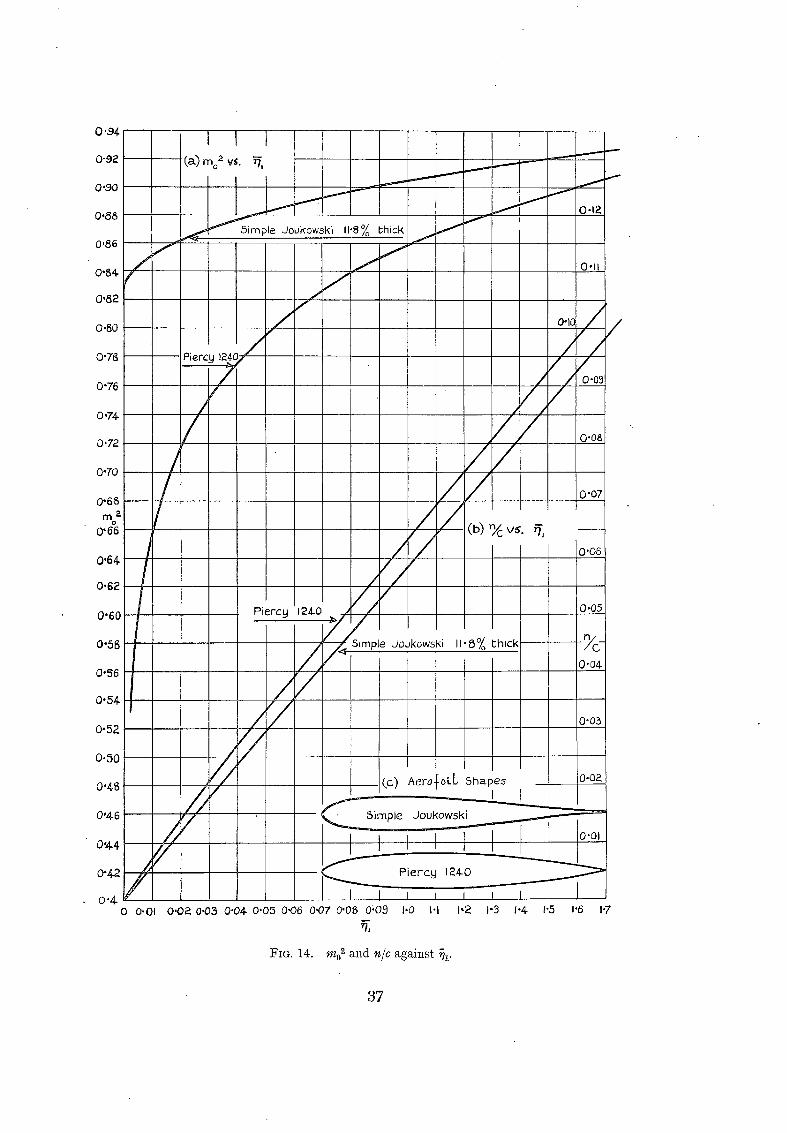
mo 2 can be computed for a given shape of basic aerofoil as a function of ~ or ~. When the aerofoil is symmetrical m0 is an e~en function of ~ or ~. I f the aerofoil is derived from the circle by a simple conformal transformation, the calculation can be made directly at chosen values of ~1 and n/C is computed from (34) where it is sufficient to write mo for m. Examples of such calculations are given in R. & M. 1996 and in Fig. 14 of this report. In the case of the arbi trary aerofoil, the velocity on the surface at zero lift must be computed by the Theodorsen-Garrick 1~ method. The aerofoil surface is treated as a vortex sheet of s t r e n g t h equal to the surface velocity, and the velocity at chosen points not on the surface is found by integration, using the method suggested in Appendix I of R. & M. 2107 and also applied to the calculation of Ay in Appendix II.

Turning now to h~ 2, this has been plotted as (h~)/Uo ~ against @~ in R. & M. 1996 for incidences of 3 deg, 6 deg and 9 deg, and for K ranging from 1.0 to 0.5. This is shown in Figs. 15, 16 and 17 Of the present 15aper. These charts are still applicable to the present report if (c~ -- c~ -- ~) = 3 deg, 6 deg, and 9 deg in turn, and with K2 = K. Unfortunately our data refer to a specific c~ (in the present report this is 6 deg) and the values of (c~ -- cq -- ~) will not be those used in the charts. However, if we imagine the boundary-layer centre-line for 6 deg and hence also (~1 + c~,) attached to other values of c¢, such that (c~ -- a~ -- ~2) = 3 deg, 6 deg, 9 deg in turn, and then find K~ for these angles, we can obtain K~ at the correct (~ -- ~.~ -- a,) by interpolation.

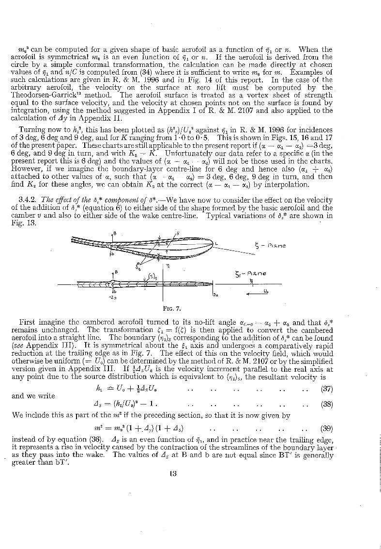
3.4.2. The effect of the ~* component of $*.--We have now to consider the effect on the velocity of the addition of C* (equation 6) to either side of the shape formed by the basic aerofoil and the camber v and also to either side of the wake centre-line. Typical variations of ~,* are shown in Fig. 13.

B -Y

~s [ / ,

( , , ,

F I G . 7 .

First imagine the cambered aerofoil turned to its no-lift angle c~L=0 = cq + c¢, and that ~s* remains unchanged. The transformation ~1 = f(~) is then applied to convert the cambered aerofoil into a straight line. The boundary (~l)s corresponding to the addition of ~s* can be found (see Appendix III). I t is symmetrical about the ~ axis and undergoes a comparatively rapid reduction at the trailing edge as in Fig. 7. The effect of this on the velocity field, which would otherwise be uniform (= Uo) can be determined by the method of R. & M. 2107 or by the simplified version given in Appendix III. If ½AsUo is the velocity increment parallel to the real axis at any point due to the source distribution which is equivalent to (~l),s, the resultant velocity is

h~ ~-- Uo + ½AsVo . . . . . . . . . . . . . (37) and we write

As = (h~/Uo) 2 - 1 . . . . . . . . . . . . . (38)

We include this as part of the m 2 if the preceding section, so that it is now given by

m 2 = m02 (1 +/]y)(1 + As) . . . . . . . . . . (39) instead of by equation (36). As is an even function of ~z, and in practice near the trailing edge, it represents a rise in velocity caused by the contraction of the streamlines of the boundary l a y e r as they pass into the wake. The values of As at B and b are not equal since BT' is generally greater than bT'.

13

3.4.3. Fina l v d o c i t y . - - T h e final veIocity h at any point outside the boundary layer along a normal at the trailing edge or other point on the surface in the plane of the aerofoil, is assumed to be given with sufficient accuracy by

h a or0 . _ rn?(1 + d , ) ( 1 + Uo ~ . . . . . . . . . . (40)

where m0 is a function of ~7~, determined by the basic aerofoil shape only, Ay is an odd function of ~1, depending on the camber y, As is an even function of ~, depending on Ys, and h,=/Uo ~ is a function of ~,, (c~ -- cq -- c~) and K,, which is given by charts, Figs. 15, 16 and 17 or from the formulae of Appendix I of R. & M. 1996.

The distance of the points ]3, b (marking the edge of the boundary layer) irom T * the effective trailing edge (Fig. 5) are given by equation 18, so from the graphs connecting n/C with '71 -- equation 34 and Fig. (14), we can determine (~h)~ and (~1)~. Thus we can obtain (h/Uo)v 2 and (h/Uo)~ 2 for various K= at { ~ - - ( c ~ - / c ~ ) } = 3 d e g , 6deg and 9deg. (Figs. 15, 16 and 17) and we put (ha/ho) ~ = (UB/U~) ~, where the value of U ~ / U ~ -"- 1.0 is taken from experiment or assumed equal to 1.0. Hence K~ can be found for {~ -- (c~ + c~)} = 3 deg, 6 deg and 9 deg. The value of (~, + c~=) corresponding to the chosen c~ of the basic aerofoil is obtained from the boundary- layer centre-line d~* and so the value K,~ can be found by interpolation. When K2 has been found it is a simple mat ter to obtain the velocities at the points B, b at the edge of the boundary !ayer at the trailing edge for comparison with those found by experiment.

8.5. The L i f t . - - T h e circulation/~ is found from

1" = K ~ g J ' o . . . . . . . . . . . . . . (19)

/'o = 4=aUo sin oc . . . . . . . . . . . . . . (27) and since

L = pUoY . . . . . . . . . . . . . . (14)

CL = (CL)oK1K2, • . . . . . . . . . . . . . (41) where

a

(CL)0 = 8= ~ sin ~. . . . . . . . . . . . . . . . (42)

4. Exper imenta l D a t a . - - I n order to avoid errors in d* and 0, which may arise from attempting their prediction from turbulent boundary-layer theory and which might mask any shortcomings of the theory as set out ill the preceding sections, it was decided to take 6" and ~ from experiments on two very different aerofoils. Both aerofoils were symmetrical, about 12 per cent thick and were derived from the circle by simple conformal transformations. One was a simple Joukowski aerofoil with a cusped trailing edge and maximum thickness at 25 per cent. The other was a Piercy aerofoil with its maximum thickness at 40 per cent and a finite trailing edge angle of 22.15 deg. The experiments are described in R. & M. 1998 (Preston and Sweeting) and in R. & M. 2013 (Preston, Sweeting, and Cox). Measurements of ~*: and d over the rear and in the wakes of the aerofoils at an incidence of 6 deg are available. The lift was also measured under approximately infinite stream conditions, so a direct comparison with tile predicted values is possible. Figs. 9 to 12 show these data plotted as functions of x/C measured from the leading edge. Also shown are the centre line ~*, camber y and thickness effects ds* of the displacement thickness ~*.Oe* in the wake, it should be noted, is relative to the line of minimum velocity.

• The position of the line of minimum velocity relative to the chord line produced was not determined in the experiments quoted, owing to the unsui tabi l i ty of the traverse gear. The discontinuity in the slope of de* at the trailing edge, therefore, may not exist and in any case the wake values are not required except to determine de* with better accuracy at the trailing edge. In addition the function H = 6*/0 is plotted and also ~*/C for the two aerofoils at ~ = 0 deg for comparison with the mean displacement thickness for 6 deg (Fig. 13). The lack of experimental poin ts over the forepart of the aerofoil necessitated approximate calculations for this region, but it was apparent later that errors in this region are not important. A more serious difficulty

14

occurs at the trailing edge, where ~* and d change rapidly. I t was assumed in interpreting the experimental data, that, up to the trailing edge, ~* and ~ increase steadily. T h i s is supported by some recent American experiments described by Mendelsohn, N.A.C.A.T.N. 1304 (1947), and any theoretical predictions based on the momentum equation would almost certainly give this behaviour. The lower surface of the Joukowski aerofoil is an exception, since laminar separation occurs near this point. The true values of ~* at the trailing edge were computed and are shown and the centre-lines and cambers based on these are also shown. The difference of shape between the two aerofoils clearly has a very marked effect on the development of ~* and 0, on the magnitude of the boundary-layer centre-line, on the maximum camber and its position and on the thickness effect of the boundary layer. In fact, one can infer from these features that the Piercy 1240 aerofoil may be expected to have a smaller lift and a more positive hinge moment than the Joukowski aerofoil.

The ratios of the experimental lift to the theoretical (potential flow) lift, corrected for the effect of the bounday layers on the side walls of tunnel were : - -

(C~)oxp~,. = 0.882 Simple Joukowski (CL)o c~ = 6 def.

(CL)expt,. = 0.695 Piercy 1240 (wires) (CL)0

The experimental ratios of the (velocity) 2 on the two sides of the aerofoil at the edge of the boundary layer at the trailing edge were : - -

UB 2 Simple Joukowski U~ = 1"023

c~ = 6 deg. UB 2

Piercy 1240 (wires) Ub2 ---- 1.000

The experimental (velocity) 2 at these points, corrected for the blockage caused by the mixing of the aerofoil boundary layer with the wind-tunnel wall boundary layer, were : - -

E = o . 9 1 5

Simple Joukowski

Piercy ( U0 / =

Uo/ = 0 . 8 9 3

( ~ / = 0 . 8 6 0 .

The blockage correction was determined by comparing the experimental pressures in the wake with those for theory using the experimental circulation, where from R. & M. 2107 there are strong reasons for believing that at about 0 .1C behind the trailing edge the two distributions should run together if there were no blockage. This consideration gave corrections on the exper{mental (velocity) 2 in the tunnel of amounts - -0 .03 for the simple Joukowski aerofoil and - -0 .04 for the Piercy aerofoil.

5. Calculations.--Calculations of m0 as a function of ~1 were already available for the two aerofoils considered here and details of the methods employed are given in R. & M. 1996. Note tha t the present notation differs from that of R. & M. 1996.

In computing ~/C as a function of ~1 from equation (34) it was found that m 2 could be replaced by mo ~ with sufficient accuracy for present calculations. Curves of m0 ~ and n/C as functions of ,71 are given in Fig. 14.

hl~/Uo 2 (in the plane of the plate) as a function of ~1 has been computed and plotted on charts in R. & M. 1996. The charts are reproduced here in Figs. 15, 16 and 17 for K~ ranging from 1.0 to 0" 50 and for c~ -- cq -- e2 = 3 deg, 6 deg, and 9 deg.

15

The ' t r u e ' values of O*/c at the trailing edge were nex tcomputed , as shown in Appendix I, equation 16 from the faired ' approximate ' O*/c and from ~/c at the trailing edge, which are shown in Figs. 9 to 12. The centre-lines ~*/c and camber lines y based on the approximate and true values of d*/c at the trailing edge were then obtained by equations 5 and 9. They are shown in Figs. 9 and 11. The lift calculations have been carried through for both sets of curves-- the approximate being indicated by I and the true by II.

The angles cq (equation 8) and c~ (equation 12) were next computed and from these K1 (equation 11) Was found.

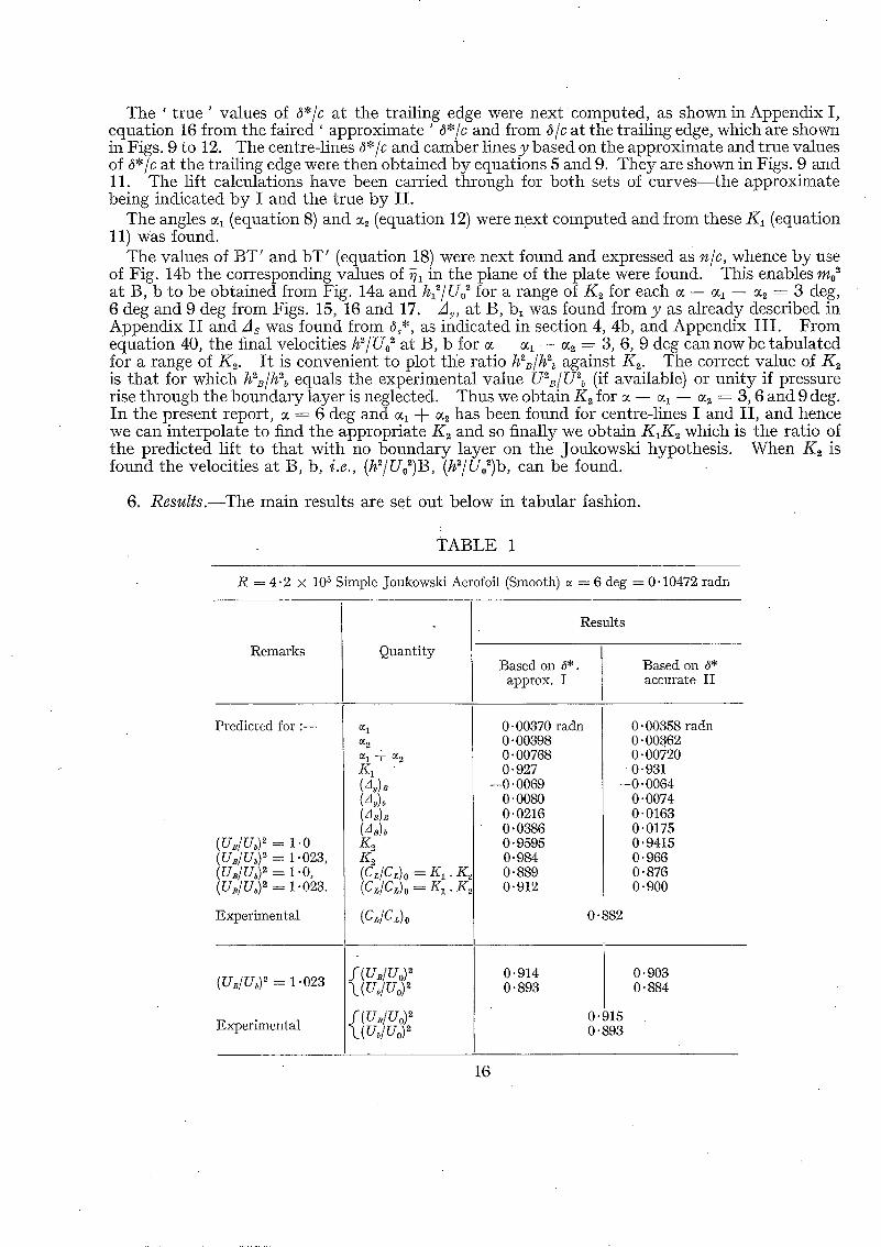
The values of BT' and bT' (equation 18) were next found and expressed as n/c, whence by use of Fig. 14b the corresponding values of ~ in the plane of the plate were found. This enables m0 ~ at B, b to be obtained from Fig. 14a and h~2/Uo ~ for a range of K~ for each c~ -- cq -- cq = 3 deg, 6 deg and 9 deg from Figs. 15, 16 and 17. A~,, at B, b~ was found from y as already described in Appendix II and As was found from d,*, as indicated in section 4, 4b, and Appendix III. From equation 40, t he final velocities h2/Uo 2 at B, b for ~ -- ~ -- ~ = 3, 6, 9 deg can nowbe tabulated for a range of K2. It is convenient to plot tl~e ratio h2~/h~ against K~. The correct value of/£2 is that for which h~B/h~b equals the experimental value U2~/U~v (if available) or unity if pressure rise through the boundary layer is neglected. Thus we obtain K~ for ~ -- ~ -- c¢2 = 3, 6 and 9 deg. In the present report, ~ = 6 deg and ~ + c¢~ has been found for centre-lines I and II, and hence wecan interpolate to find the appropriate K2 and so finally we obtain K1K2 which is the ratio of the predicted lift to that with no boundary layer on the Joukowski hypothesis. When K~ is found the velocities at B, b, i.e., (h'~/Uo2)B, (h2/Uo2)b, can be found.

6. Resul t s . - -The main results are set out below in tabular fashion.

TABLE 1

R = 4 . 2 × 10 a Simple Joukowski Aerofoil (Smooth) e = 6 deg = 0" 10472 radn

Remarks Quan t i t y

Resul ts

Based on ~*. approx. I

Based on 8" accurate I I

Pred ic ted for : - -

(UB/U~) 2 -- 1.0 (U~/Ub) ~ = 1-023, (UdU,)~ = 1 "0, (UdU~) ~ = 1.023.

Expe r imen ta l

(UB/Ub) ~ = 1 "023

Expe r imen ta l

0:2 0:1 "~- 0:2 Iq (~). (A,)~

(~)~ K2 K2 (cdC~)o = K1. K~ (Cz /Cz)o = K 1 . K 2

(cdC~)o

f (uduo)~ \ (Ub/UoV

f(UdUoP \(VblUo) ~

0.00370 radn 0.00398 0.00768 0-927

- -0 .0069 0.0080 0.0216 0.0386 0.9595 0.984 0.889 0 .912

0 .914 0 .893

0"00358 radu 0.00362 0.00720

0 . 9 3 1 --0-0064

0.0074 0.0163 0.0175 0.9415 0 .966 0.876 0.900

0.882

0.903 0"884

0 .915 0 .893

16

TABLE 2

R = 4.2 × 10 ~ Piercy 1240 Aerofoil (Turbulence Wires) ~ = 6 deg = 0-10472 radn

Remarks Quantity

Results

Based on d* approx I

Based on 6* accurate I I

Predicted for :--

( u d u , ) ~ = 1 .o ( u d u ~ ) ~ = 1 .o,

ExperimentM

Experimental

~'i ~2 ~i -~ °'2 KI

( ~ ) ~ (d~), K~ (c , /C,)o = K~ .

(c,/C)~o

(UdVo)~=(UdUo) ~ (UdUo)~=(uo/Uo) ~

0.00690 radn 0.01388 0.02078 0-802

--0-020 0.020 0.0712 0-1012 0.9515 0"763

0.00723 radn 0.01800 0.02523 0.7585

- -0 -0292 0-0338 0.0434 0.0536 0.9565 0.725

0.695

0.720 based on Bryant'sgeneralised curves.)

0.883 I 0-855 0.860

7. Discussion.--7.1. Prese~ct Results.--From Tables 1 and 2 in the columns giving the results based on the accurate values of ~*, it is seen that in the case of the simple Joukowski aerofoil the predicted CL/(CL)0 = 0"900 is greater than the experimental CL(CL)0 = 0.882 by about two per cent, while for the Piercy aerofoil the predicted CL/(CL)0 = 0" 725 is greater than the experimental CL/(CL)0 = 0.695, by about four per cent. For this aerofoil at R ---- 4.2 × 105 using generalised curves given by Bryant (15) correlating experimental results on a trailing-edge angle basis, we should expect an experimental CL/(CL)0 ---- 0.72, so that the predicted value is in good agreement with this estimate. It is difficult to say whether the fact that the predicted values of CL/(CL)0 are slightly greater than the measured values is of significance. There is the possibility of small errors in the

• experimental value of ~*, $ and in the lift itself. The aerofoils used in the tests may not have accurately reproduced the theoretical shape in the region of the trailing edge. There is the difficulty that ~* and ~ at the trailing edge were not well defined experimentally and the calculated values of CL depend on the interpretation of the measured values here. In addition, the factors Ay, As were not computed to a high accuracy because of the labour involved and the lack of precision in ~* and ~ near the trailing edge. In view of all these possible inaccuracies, it is considered that the predicted lifts are in satisfactory agreement with experimental results.

A further check on the method of calculation is furnished by the comparison of the velocities at the points B, b at the edge of the boundary lkyer at the trailing edge. Tables 1 and 2 show the predicted and measured (velocity) ~ to be in good agreement. This, at least, suggests that the theory, governing the deduction of 8" accurate and the the calculation of A s on which the velocity at B or b depends, is satisfactory.

The importance of the boundary-layer incidence and camber effect is shown by the values of ~1 and ~2 in relation to c~ and by the value of K1 in Tables 1 and 2. The departure of the predicted lift from the Kutta-Joukowski value with no boundary layer is represente~l by K1 × Ks and it is seen that K1 accounts for most of it. K~ does not differ greatly for the two aerofoils, but the values of/£1 do. From Figs. 9 and 11 showing ~c* and the camber it is seen that aerofoil shape

17 (s229s) B

has a pronounced effect. The maximum b0undary-layer camber is about 0.12 per cent for the Joukowski aerofoil and occurs at about 0.6C from the leading edge, whereas for the Piercy aerofoil which has a trailing-edge angle of 22- 15 dog, it is about 0" 34 per cent occurring at 0- 8C. This difference in camber explains in part why a cusped aerofoil with its position of maximum thickness well forward has a lift only some ten per cent less than the Kutta-Joukowski value for the aerofoil with no boundary layer, compared with the thi r ty per cent reduction suffered by an aerofoil with its maximum thickness further back and a trailing-edge angle of 22.15 dog. I t also explains why plain controls on a cusped section tend to be heavily underbalanced, whereas those on a section with a large trailing-edge angle are over-balanced. However, further experiments, in which the course of the boundary layer is carefully explored near the trailing edge, are highly desirable, particularly as on cusped aerofoils the measured hinge-moment slopes apparently exceed the theoretical Joukowski values, though the lift slope is below the Joukowski value (seeBryant) 1~ This, if true, implies a reversal of boundary-layer camber near the trailing edge and therefore very rapid changes in 3" on the two surfaces in this region, which obviously increases the difficulties of calculation.

Turning now to the comparison between the calculations based on the approximate values of 3" and those using the accurate values, we note on Figs. 9b and l l b that the centre-line component (~c*) at the trailing edge is slightly less in the case of the Joukowski aerofoil and slightly greater in the case of the Piercy aerofoil when based on the accurate evaluation of d*. This difference is reflected in the camber y, Figs. 9c and 11c and in cq, ~-2, K1 and Ay, Tables 1 and 2, and illustrates the relative sensitivity of these quantities to a small change of centre line de*. As regards the thickness component Os*, Fig. 13a shows that the accurate value is considerably less than the approximate value at the trailing edge and it is presumed that a considerable rounding off of ~s* occurs in this neighbourhood, which is certainly more acceptable than the discontinuity of slope which occurs when the approximate values are taken. This rounding-off of d~* greatly reduces (As)B, (As)~ and makes their values more nearly equal. I t will be noted from Tables 1 and 2 that K1 is reduced by increase of ~c* at the trailing edge, but because (A,)~, (A Y)b have their values numerically increased the effect of this is to increase K~. On the other hand the evening up of the values of (Ay)~ (Ay)~ tends to reduce K~, so that no great change of K, takes place. Also, the predicted values of the (velocity)" at B, b have come out greater for the calculations using 3" approx. The increments A r, A s, though troublesome to calculate, cannot be neglected in general. For theJoukowski aerofoil, their neglect would not be serious and, in fact, would lead to a reduction in (CL/Cc)o of about two per cent. In the case of the Piercy aerofoil their neglect would lead to a reduction in (CL/CL)o of about eleven per cent, thus bringing the calculated value well below the experimental value . The (velocity) ~ at the points B, b at the edge of the boundary

layer would come out too low by a factor" [ 1 -- (As)3 ~- (As)b. ] " 2

In the present calculations, we have fixed the circulation by making the calculated velocity ratio (hB/hb) ~ = (U~/Ub) ~, the experimental velocity ratio. Neglect of curvature or, what amounts to the same thing, of pressure rise through the boundary layer gives (ha/h~)" = 1.00 for no net discharge of vorticity into the wake. In the case of the Joukowski aerofoil the ratio (U~/Ub)~= 1.023 from experiment, but in the case of the Piercy (U~/Ub) ~ = 1.00. The pressure rise through either boundary layer at the trailing edge i s 'certainly greater for the Piercy aerofoil than for the Joukowski aerofoil, but it so happens that the rise for the two sides is the same. This difference for the ratio (U~/Ub) ~ is probably related to the totally different behaviour of 3" for the lower surface near the trailing edge for the two aerofoils, Figs. 9a and l l a . There would be no difficulty in computing the pressure rise if the curvature of the streamlines and t he velocity distribution along a normal to the trailing edge were known. However; in view of the closeness of the experimental ratio (Uv/Ub) 2 to uni ty it would be quicker to conduct experiments for aerofoils with different trailing edge angles and to relate the pressure rise to the boundary layer thickness and the trailing edge angle in an empirical manner. A change in (UB/U~) 2 from 1.0 to 1.023 is shown in Table 1 for the simple Joukowski aerofoil, where it is seen that CL/(CL)o is increased by about two per cent. A similar change in (UB/Ub) ~ for the Piercy aerofoil would lead to a slightly

18

greater change of lift. I t appears from experimental data that (UB/Uv) ~ > 1.0 for cusped aerofoils, but as the trailing-edge angle gets large (UB/U~) ~ < 1.0 and from comparison with other aerofoils (U~/U~) ~ = 0.995 might have been more acceptable for the Piercy aerofoil, thus giving a slightly smaller CL/(Ci)o in Table 2.

7.2. Ge~eraZ Comme~ets.--The essence of the work described in this report is the calculation of the potential flow which effectively exists outside the boundary layer and wake. We seek a shape which, when added to the aerofoil, is such that the potential flow streamlines about the combined shape cross the line representing the edge of the boundary layer and wake at the angle which the streamlines cross in the real flow. Hence, outside the boundary layer and wake the fictitious and real flows are identical. Inside the boundary layer and wake we must appeal to boundary-layer theory or to experiment if we wish to obtain details of the flow. I t may be noted tha t no at tempt was made to fix the position of the wake, it being left flee to set itself along the general direction of the ftow about the aerofoil plus boundary-layer centre-lille. Use was made of the idea of displacement flux in determining the additive shape which represents the effect of the boundary layer and wake, and the subsequent calculations were simplified by the introduction of symmetrical and antisymmetrical contributions of this shape to the aerofoil and by the use of thin aerofoil theory, involving vortex sheet theory and sources and sinks.

In R. & M. 2107, two additional methods were tried in the calculation of the effect of the boundary layer and wake on the flow past a symmetrical aerofoil at 0 deg incidence. In one, the vorticity at any section of the boundary layer was imagined to be concentrated at its centre of gravity in the form of a vortex sheet, and the contribution of this to the flow past the aerofoil with no boundary layer was determined for points lying outside the line representing the edge of the boundary layer and wake. In the other method, the actual distribution of the vorticity in the boundary layer and wake was used. Both these methods gave results in close agreement with the method employing a source-sink representation of t he ' displacement flux '. The approximate condition for no net flux of vorticity into the wake, namely, that the velocities at the edge of the boundary layer on the normal to the streamlines at the trailing edge are equal, makes the accuracy of the lift calculation, in part, dependent on the accuracy of calculation of these velocities. These alternative methods could be employed in the case of the lifting aerofoil and would form a check on the velocity calculations at the edge of the boundary layer at the trailing edge, provided the strength of the vorticity can be obtained with sufficient accuracy in this region. The effect of trailing edge-strips described in R. & M. 1996 furnishes experimental evidence of the sensitivity of the lift to factors which affect the velocity field near the trailing edge.

The method of this report requires the definition of an actual edge to the boundary layer e.g., ~ = ~. At first sight this may appear very objectionable for calculations of the kind which have been made in this report. However, for a turbulent boundary, in practice, the definition of an actual edge can be m a d e i n a consistent manner, as there is a relatively rapid approach of the total pressure to the free stream total pressure at the edge of the boundary layer. Moreover, errors in d, in the main, only, affect the K~ factor, which does not have a decisive influence on the final value of (CL/CL),, though small errors may be present in the final tabulated values which arise from errors in d. Any objection to the use of d can be overcome by applying the vorticity condition in the form that the pressure at the trailing edge T is the same-whether approached from above or below along a normal to the streamlines, through T. The (velocity) ~, or, by Bernoulli 's theorem, the pressure is computed at points which lie outside the boundary layer for various K2. These can be transmit ted to the trailing edge if the velocity distribution and the curvature of the streamlines are known. The correct value of K~ is tha t which makes (Pr)z = (Pr), • Such calculations, of course, would be considerably more laborious than those given here and require greater knowledge of the turbulent boundary than is at present available.

8. Exte~¢sior~ of lhe Calculatior~s.--8.1. Pressure Distribution, Pitchi~g Moment and Hi~ge Mome~#s.--Having determined the circulation, the next step is to compute the velocities or. pressures at the edge of the boundary layer around the aerofoil employing the method already

19 (52298) B 2

used for computing the velocities at B, b, at the trailing edge. Such calculations would be rather tedious and laborious ; however, assuming they can be carried out, the pressures have then to be transmitted through the boundary layer to the aerofoil surface. This requires a knowledge of the velocity distribution through the boundary layer and the curvature of the streamlines. Except near the trailing edge this latter may be taken as constant through the boundary layer and equal to that of the aerofoil surface. In general, this curvature is likely to be small and so the pressure rise through the boundary will be very small and may be neglected, so that over most of the aerofoil, except near the trailing edge, the velocity calculations may be carried out at the surface itself---taking due account of boundary-- layer camber and thickness effects. I t may well prove when typical calculations have been made, that even in the trailing edge region itself, judicious extrapolation from the region where the curvature is small to the trailing edge where the pressure can be found, will suffice. Comparison of calculated and measured pressures at the surface will provide a severe test for the basic theory and the methods of calculation set out here.

The pitching moment and hinge moments can then be found by taking moments and integrating. The latter are the most likely to be seriously affected by errors in the surface pressures near the trailing edge.

8.2. Scale Effects.--The present calculations have been carried through with boundary-layer data taken from experiment and in section 8.1 it has been indicated how the velocities at the edge of the boundary layer and the surface pressures may be found. Given the velocity at the edge of the boundary layer and fixing the position of the transition points, and the Reynolds number, there is no difficulty in calculating the displacement thickness of the laminar boundary layer. The turbulent boundary layer can be calculated by semi-empirical methods such as that developed by Doenhoff and Tetervin 16 or the simpler version developed by Garner (R. & M. 2133). These are probably sufficiently accurate provided the separation position is not too closely approached and the curvature effects near the trailing edge (pressure rise through the boundary layer) are not large. Thus the displacement thickness on the usual definition can be found for either surface as far as the trailing edge. As regards the course of the displacement thickness in the wake there is at present no theory enabling this to be computed, but the momentum thickness 0 can be found with sufficient accuracy and, therefore, in order to compute displacement thickness H = d*/0 must be found. A limited appeal to experiment should suffice to determine H empirically, as H is known at the trailing edge and far down the wake it tends to 1- 0. In any case, no great accuracy is required as this only affects the factor As and this has no decisive effect on the circulation.

To start the calculation it is necessary to guess the circulation or take the Joukowski value. The potential flow velocity at the edge of the boundary may be taken as that at the surface--with a suitable guess at the trailing edge--the velocities here being taken as equal. The boundary- layer displacement thickness can, therefore, be found for both surfaces and for the wake. The circulation for this boundary-layer configuration is found as described in this report and the velocity at the edge of the boundary layer is computed anew as indicated in section 8.1. From the second approximation to the velocity distribution a second approximation to the displacement thickness is found, and the corresponding circulation is found which should be sufficiently accurate. Further iterations can, of course, be carried out if found to be necessary.

This operation can be repeated for otlqer transition positions and Reynolds numbers and so, for a given wing, it should be possible to predict the sectional characteristic for incidences below the stall.

Prediction of the stall requires further development of the turbulent boundaryqayer theory, as turbulent separation is not thought to be given with sufficient precision by existing theories. Moreover, little or no information exists on the behaviour of the boundary layer downstream of a turbulent separation. I t will be evidence that as stalling incidence is reached, the upper boundary, layer and the wake will be very thick and exert a considerable effect on the velocity field. The relatively crude calculations of Refs. 2 and 3 show that prediction of the stall is by no means hopeless, but considerable experimentM investigations of the boundary-layer flow in this regime of incidence must be undertaken before such cMculations can have any practical value.

20

8.3. Mach Effects.--The basic theorem relating to the constancy of circulation r in circuits enclosing the aerofoil and its boundary layer and which cut the streamlines in the wake at right- angles, the result that the net flux of vorticity into the wake at the trailing edge is zero and the relation

L ---- poUoP,

where p0, U0 refer to the stream at infinity, have not involved the continuity relation and hence are true for compressible flow (see Temple°).

The velocity field is, of course, affected by compressibility and the boundary layer will also be affected. The laminar boundary layer can probably be calculated for compressible flow with. sufficient accuracy. The tubulent boundary layer has not yet received much attention, but the calculation by Young and Winterbottom (R. & M. 2400) represents a start in this direction. In R. & M. 1996 the assumption was made that the boundary-layer configuration was not affected by Mach number. I t was then deduced that the circulation as predicted, taking account of the boundary layer, would be affected by Mach number in exactly the same way as the Joukowski value for potential flow. This is still true for the calculations of the present report. As experiment, in many cases, confirms this up the critical Mach number, it is concluded that Mach effects on the boundary-layer thickness are small and hence relatively crude calculations of these effects might suffice.

I t would, therefore, appear that calculation of Mach effects up to the shock stall should be possible if the necessary extensions to turbulent boundary-layer theory can be made and checked experimentally.

9. Conclusions.--The calculations made in this paper show that satisfactory agreement has been obtained between predicted and measured lifts and between predicted and measured velocities at the edge of the boundary layer at the trailing edge for two quite different aerofoils. The differences which exist may be ascribed in part to possible errors in the measured values and in part to the interpretation put on tile experimental data which were used in the calculations, and also to the fact that these data did not warrant more accurate, but laborious calculations of the effects of the displacement thickness on the velocities at the edge of the boundary layer.

In contrast to the calculations of R. & 1K. 1996 and those of Nitzberg 10, the calculations made here are free from empiricism and they have a sound theoretical basis. In the former the effects of the boundary camber and incidence were neglected and in the latter no at tempt was made to satisfy the condition tha t there is no net flux of vorticity into the wake at the trailing edge. In this paper the basic ideas behind these previous two methods of predicting lift have been harmonised and I believe, in the broad sense, the result gives the correct method of approach to the problem, though the detailed calculations may possibly be improved.

Successful application of the method is dependent on the accuracy with which the boundary- layer cambe r and incidence can be predicted and on the accuracy of the calculation of the velocities at the edge of the boundary layer at the trailing edge.

The importance of boundary-layer camber and incidence effects is well brought out in this paper and they account for most of tile drop of lift from the Joukowski value. The present calculations have utilised boundary-layer data taken from experiment and there is an element of uncertainty about these in the region of the trailing edge, which is sufficient to warrant further experimental investigations on large models in this region. Such data should be used to check existing turbulent boundary-layer theory, since the accuracy of ab initio calculations of lift and other characteristics will depend on the accuracy with which the turbulent boundary-layer characteristics can be predicted, particularly near the trailing edge, where curvature effects are becoming important.

The methods given in the appendices of calculating the velocity at the edge of the boundary l a y e r might possibly be reviewed, particularly those which deal with the effect of the boundary layer, as distinct from aerofoil effects. The camber and thickness contributions of the displacement thickness change rather rapidly in the region of tile trailing edge and some inaccuracy is

21

probably incurred by the present methods. As regards the contribution to the velocity made by the aerofoil, the charts of Figs. 15, 16 and 17 should be extended to cover 1 deg intervals of (c~ -- cq-- c~2) in order to make interpolation easier.

Having found the circulation there should be no difficulty in computing the pressures at the surface, except near the trailing edge where further research is needed to see how this can be done quickly and with sufficient accuracy. The pitching moment and hinge moment can then be found.

I t would thus appear that for incidences below the stall we should be able, on existing turbulent boundaryvlayer theory, to calculate approximately the effect of transition position and Reynolds number on all the major sectional characteristics of an aerofoil. The stall (above the first appearance of turbulent separation) will require further experimental investigation and extension of turbulent boundary-layer theory and possibly refinement of the calculations set out in this paper. In addition, if the necessary extensions to present turbulent boundary theory can be made, we should also be able to predict the effect of Mach number on these characteristics up to the critical Mach number. These calculations, of course, represent a lengthy undertaking even for one aerofoil, but they would amply repay the labour by increasing our knowledge of the part played by these variables on the behaviour of sectional characteristics, and possibly lead to shorter methods of prediction which would be more suitable for routine investigations.

22

No.

1

2

3

4

Author

H. B. Squire and A. D. Young

L. t towarth . . . .

• °

• °

N. A. V. Piercy, J. H. Preston and L. G. Whitehead

j . I-I. Preston . . .~ ..

5 L . W . Bryant and D. H. Williams

6 G. Temple . . . . . . . .

7 J. I-I. Preston .. . . . .

8 J. Striper . . . . . . . .

9 R. ~ . Pinkerton . . . . . .

10 G. 17;. Nitzberg . . . . . .

11 H. Glauert . . . . . . . .

12 T. Theodorsen and I. E. Garrick

13 J . H . Preston and N. E. Sweeting

14 j . H. Preston, N. E. Sweeting and D. Cox

15 L . W . Bryant . . . . . .

16 A.E. von Doenhoff and N. Tetervin

17 H .C . Garner . . . . . .

18 A .D . Young and N. E. Winterbottom

19 H. Lamb . . . . . . . .

20 W . L . Cowley and H. Levy ..

REFERENCES

Title, etc.

The Calculation of the Profile Drag of Aerofoils. R. & lVl. 1838. 1937.

The Theoretical Determination of the Lift Coefficient of a Thin Elliptic Cylinder. Proc. Roy. Soc. A, 149, pp. 558-586. 1935.

The Approximate Prediction of Skin Friction and Lift. ,Phil. Mag. XXVI, p. 791. 1938.

The Approximate Calculation of the Lift of Symmetrical Aerofoils taking account of the Boundary Layer, with Application to Control Problems. R. & M. 1996. 1943.

An Investigation of the Flow of Air Around an Aerofoil of Infinite Span with an Appendix by G. I. Taylor. R. & M. 989. 1924. Also Phil. Trans. Roy. Soc. A, 225. 1925.

Vorticity Transport and Theory of the Wake. A.R.C. 7118. 1943. (Unpublished.)

The Effect of the Boundary Layer and Wake on the Flow Past a Sym- metrical Aerofoil at Zero Incidence. R. & M. 2107. 1945.

Auftriebsverminderung eines Flfigels durch seinen Widerstand. Z.F.M. 24, pp. 439-441. 1933,

Calculated and Measured Pressnre Distributions over the ~idspan Section of NACA 4412 Aerofoil. N.A.C.A.T.R. 563. 1936.

The Theoretical Calculation of Airfoil Section Coefficients at Large Reynolds Numbers. A.C.R. 4112. 1944.

EIeme~#s of Aerofoil a~¢d Airscrew Theory. 2nd edit. Camb. Univ. Press.

General Potential Theory of Arbitrary Wing Sections. N.A.C.A.T.R. 352. 1933.

The Experimental Determination of the Boundary Layer a n d Wake Characteristics of a Simple Joukowsld Aerofoil, with Particular Reference to the Trailing Edge Region. R. & M. 1998. 1934.

The Experimental Determination of the Boundary Layer and Wake Characteristics of a Piercy 12/40 Aerofoil, with Particular Reference to the Trailing Edge Region. R. & M. 2013. 1945.

Two Dimensional Control Characteristics. Lift Due to Plain Flap. A.R.C. 9534. 1947. (To be published.)

Determination of General Relations for Behaviour of Turbulent Boundary Layers. N.A.C.A.T.R. 772. 1943.

The Development of Turbulent Boundary Layers. R. & M. 2133. 1944.

Note on the Effect of Compressibility on the Profile Drag of Aerofoils in the Absence of Shock Waves. R. & 1~{. 2400. 3/Iay, 1940.

Hydrodynamics. 6th Edition. Paragraph 328a.

An Analysis of the Steady Two-Dimensional Flow of an Incompressible Viscous Fluid. R. & 5~. 715.

23

APPENDIX I

Calculation o] the True Di@lacement Thickness

1. Conditions at the Edge of the Boundary Layer . - -Take a system of curvilinear co-ordinates cd, /3', defined by the equi-potentials and the streamlines of the potential flow about the basic aeroIoil, with the Joukowski value of the circulation. ~', and /3' are identical with c~ and /3 as used in R. & M. 1996, the dashes being added to avoid confusion with c~ and/3 as used in the early part of this report to indicate angles.

Let h0 be the velocity of potential flow for the basic aerofoil with no boundary layer, and ds, dn the lengths of the sides of the element d~', d/3' in the plane of the aerofoil.

Then ho . ds = dcd

. . . . . . . . . . . . . . ( 1 ) ho . dn = d/3'

Let q, w be the velocity components along the lines /3' = const, and ~' = const, through any point for the real flow past the aerofoil. Then from Appendix I of R. & M. 1996, the equation of continuity is

~c2 a ~ as--' + a/3' - O, . . . . . . . . . . . . . . (2)

where = q/ho ]

= ~ /ho / . . . . . . . . . . . . . . . (a)

Let /3~' be the value of/3' corresponding to the edge of the boundary layer n = ~. equation (2) above

= Vo - - ~ ,

Then from

d ' d&' ffo~ q d/3' + q~ dc~ ,

d " d&' - Vo ° (1 - e l 3 ' - - (1 - - ol. (4)

The angle which the real streamlines make with those of potential flow defined by/3 ' at /3' = & is

4 zG 1 d, ~' -- q-L q= ~ ( 1 - q)d/3'-- d~' (1--4)~ " ""

= const,

. . (s)

Now as a good approximation, when the boundary layer is ichin and the circulation does not differ much from the Joukowski value

¢~ = V ---- (ho)~, i.e.,

q~ ~ 1 .0 .

24

Hence {o this degree of approximation, equation (5) may t~e written

d - | 4 (1 - ~) d~'

8 f (h0 -- q) dn

- - d o ~ t o

d - d ~ ' ( ~ * ) ' " . . . . . . . . .

by definition

(see equation :3, section 4).

#

i 4 (6)

d 1 d = T~ ' (~*) - h ~ d ~ (~*) . . . . . . . . . . . (8)

Now from R. & M. 2107, the appropriate source strength which deflects the streamlines of the required potential flow through this angle is

d Q = ~ ( ~ * ) d ~ ; . . . . . . . . . . . . (9)

these sources being distributed along the part of the real axis representing the aerofoil in the ¢2-plane and along the dividing streamline, which springs from the trailing edge of the plate. Now the source strength is unaffected by the transformation and (9) may be written

1 d (? - h~ dS~ (~*) h~. de~

d (~,) a~' . . . . . . . . . . (~0) - - d o l t • . .

25

a n d so

Now outside the boundary layer a 'potential flow exists, which differs slightly from that for the aerofoil with no boundary layer. The inner boundary condition for the flow is tha t the streamlines enter the boundary layer at n = ~ or ~' = ~e' making an angle 6 (equation 6) with the line /~' = const., at this position. If this inner boundary condition can be satisfied, together with external boundary condition, which is fixed by the flow at infinity, then the flow outside the boundary layer is the correct one when the boundary layer is present.

2. Method of Computing the Effect of the Boundary Layef<.--Transform the basic aerofoil into a straight, line by ~ = f0(~) and let /

/7/

where the C-plane is the plane of the aerofoiI and the ¢2-plane is that of the straight line. If h~ is the velocity in ¢~-plane and h0 is the velocity in the C-plane, ignoring boundary-layer effects then

h0 = h~. m0. I f

G = G + i ~ ,

the straight line into which the aerofoil is transformed forms part of the real axis

~ = O.

The angle $ (equation 6), at points on ~ = (~)~ in the C2-plane corresponding to points on ~ = or $ ' = ¢?~' in the C-plane, is unchanged by the transformation.

Now near the boundary d~ ' = h0 (ds),,=0 = h~. d ~ ,

K n o w i n g ~*, we could, as in R. & M. 2107, proceed to compute the velocity increment due to this source distribution at required points on or outside the edge of the boundary layer. I t is, however, more convenient to compute the equivalent change of aerofoil shape which will produce the same effect and to break up this change of shape into a change of centre-line plus equal contributions of thickness to the two sides of the aerofoil.

3. Equivalent Change of S h a p e - - T r u e Di@lacement T h i c k n e s s . - - T h e boundar.y formed by the closing streamline when the sources (equation 9) are introduced in the ~-plane, is given (see R. & M. 2i07) by

~0" . . . . . . . . . . . . . . (11)

since, for 0 < ~ < (~2)~, h2, even near the trailing edge, is very closely Constant, for all incidences, since curvature has been almost removed by the transformation. The boundary formed by the closing streamlines in the aerofoil or C-plane corresponding to ~2 = ~* in the G-plane will be at n = 6" say, where 6" is now the true displacement thickness. We have

ho . dn = h2 . dn2 = dot' . . . . . . . . . . . . . (12)

Hence

;7 r ho. dn = h~ .drl~ l___ h~. ~72" = ~P* . . . . . . . . . . (13) --0

from equation (11).

But by definition (see section 4, equation 3)

f° = (ho- - q) d n . o

Hence * ho. dn = ~* = , (ho - - q)dn . . . . . . . . . (14)

This may be regarded as the definition of the true displacement thickness 6*.

Over most o f the aerofoil, with the exception of the region in the immediate vicinity of the trailing edge, h0 -~ U, the experimental velocity at the edge of the boundary layer and equation (14) reduces to

2 U~* = ~* = (U - - q) dn

o r = f (1 - q /U) d n . . . . . . . . . . ( i s ) 6"

0

which is the approximate definition of 6"

At the trailing edge, instead of using (14), we can proceed as follows if 6 and 6" approx, are known. Now (equation 11)

~ * - - h~ - - h~ o (ho - - q ) d n ,

N o w

ho = h~ .mo , hence

~ 2 " = o m ° ' d n -- (6 - - 6*approx.) .

26

Now since

Or

hO drl~ = ~ dn = too. dn ,

U (3 - = approx.) .

~ * U C (3/C - - ~*/C approx.) . . . . (16) q ~ * - - 2 a - - (q~)~ - - h ~ 2a

if the aerofoil of chord c transforms into a straight line of length 4a. For h~ we take the average value for 0 < ~7~ < (q~)~.

Now at the trailing edge we have in Fig. 14b cm'ves relating q~ to n/c, hence we can find (q~)~ corresponding to n/c = ~/c. Thus we can find ~7~* and from the same figures we can read off the corresponding value of 3" true.

Note in Figs. 15, 16 and 17 that (cq + gp) in c~ -- (cq + ~-2) is put equal to 0, since we are dealing with the basic aerofoil and the curve K2 ---- 1.0 is taken since h0, g', ~" refer to the Joukowski circulation for the basic aerofoil.

In the above calculation of the true displacement thickness, it will have been noted that the direction of the real flow streamlines entering the boundary layer was found relative to the direction of the potential flow streamlines about the aerofoil with no boundary layer and with the Joukowski value of the circulation. Now, if the actual circulation differs much from the Joukowski value, the flow outside the boundary layer would be better approximated by using the actual circulation--if known. In particular, the approximation made in the analysis tha t

= U (h0)

would be most closely fulfilled. On the other hand, this would lead to difficulties in evaluating ~* true in terms of 3" approx, at the trailing edge, since the potential flow would no longer leave the trailing edge smoothly and very rapid changes of the potential flow velocity would occur.

Now, except near the trailing edge, d* true and ~* approx, should be the same very closely and the assumption

= u (ho)o,

when (h0) is now supposed constant over a distance comparable with 3, leads to this result, though as already mentioned, this assumption would be more closely fulfilled if the actual circulation or a good approximation to it were used. If we retain the Joukowski circulation, we will have to consider the accuracy of the calculation of 3" true at the trailing edge.

The results deduced by the method of calculation set out above show that the centre-line contribution 3,* is very little different from the value based on the approximate definition. Now 3°* via K, is responsible for the greater part of the loss of lift below the Joukowski value. Hence if we took the aerofoil with the centre-line, found in the approximate basis, and the Joukowski value of the circulation appropriate to the centre-line, e.g., K ~ . Fo the potent ia l flow would leave T' smoothly, and since this circulation does not differ much from the actual circulation, tile assumption that the actual velocities at the edge of the boundary layer ate equal to the potential flow velocities at this position would now b'e more closely fulfilled. No essential change of procedure would be required in finding ~* true other than to note that the modulus of transformation from the aerofoil plus to boundary-layer centre-line to the plane of the plate would differ slightly from tha t for the aerofoil only, to the plate. For the cases dealt with this is small and would only affect the value of ~* true very slightly. Hence it is concluded that the calculations of (~* true) based on the use of the Joukowski circulation about the basic aerofoil are sufficiently accurate.

27

A P P E N D I X II

Calculation o/ Ay

Here we are ignoring the presence of a*s and are concerned only with the camber y.

Ay is the factor which is related to the velocity increments arising from the boundary-layer camber y. If the transformation G = f(¢) is applied so that the aerofoil plus camber line in the g-plane becomes a straight line in the ¢,-plane, then from section 8.4, equations (29) and (86)

h ~ = m2hl 2

= m0~(1 + A,)h? . . . . . . . . . . . (1)

If the aerofoil plus boundary-layer centre-line is placed at its no-lift incidence

then it follows from section 3.4 that

h ? - - Uo . . . . . . . . . . and from (1) and (2)

h ~ = mo~(1 + A,)Uo ~ . . . . . . . . .

(2)

(3)

Apply the transformation ¢= = f0(¢)

to the aerofoil plus camber line in the g-plane, so that the basic aerofoil transforms into a straight line in the g=-plane. Then,

m°~= ~ . . . . . . . . . . . . (4)

The aerofoil plus the boundary-layer camber line y will give very closely in the g-plane a camber line only, whose shape (provided the basic aerofoil is thin) is almost identical with the camber line y in the plane of the aerofoil. We assume that the camber lines are identical.

If h2"is the velocity in the new ¢2-plane, then, when the aerofoil plus camber line is at its no-lift position and since

h ~ .= mo~h~ ~ , it follows from (3) that

u0 (1 + . . . . . . . . . . . . . (5) Hence if we can compute h, 2 at desired points, we can obtain A, from equation (5). Now the camber line in the ¢~-plane is at its no-lift incidence and it is in effect a vortex sheet, we can compute its strength k by applying the thin aerofoil theory of Glauert 1. or by use of the Theodorsen- Garrick 1~ method.

P

~.a~ ~ - ~

ac ~ l-ac

FIG. 8.

The velocity at the camber line is given by

h 2 = Uo ± k / 2 .

The velocity at points not on the camber line can be obtained when the strength of the vortex sheet has been found. If the camber is small, then as in Glauert's thin aerofoil theory, we can take the vortex sheet along the chord line.

28

The circulation round an elementary vortex forming part of the vortex sheet is k dx and with notation of the figure the velocity at a point P on the normal to the chord at the trailing edge is

kdx d q - 2ar . . . . . . . . (7)

where r" = (2 -- x)" + y2

I t has components

d~ = dq x sin 0 - -

kdx x y 27~72

dv = -- dq X cos 0 = k d ~ x ( l - x )

27~r 2

(s)

Whence by integration y fl k dx

u = o (1 - x) ~ + y~

1 fl k(1--x) dx v = ~ 0(~ _ x)2 + y ~

(9)

If u, v are small compared with the stream velocity Uo, then

h ? = (Uo + u) 2 + v ~ ~- Uo~(1 + 2u/Uo) . . . . . . . . (10) and

2u y /~ k dx A Y - - u o - - a U o 0 ( l - - x ) ~ + y " . . . . . . . . . (11)

Now k is the strength of the vortex sheet at the no-lift incidence of the camber line. I t can be considered as the sum of two distributions--one corresponding to the optimum incidence aopt of the camber line in which k is finite everywhere, and the other giving a distribution proportional to

-- ~opt and varying as cot ¢/2 where ¢ = cos -1 (1 -- 2x). This is the flat plate distribution and yields an infinite value for k at the leading edge x = 0 = 0. The contribution to Ay for this distribution can be obtained from the charts (Figs. 15, 16 and 17) by intert~olation for the particular value of ~ -- ~opt and using the curves K, = 1.0. Hence we must find c%t for the camber line by thin aerofoil theory or otherwise.

The contribution to Ay from the ~opt distribution must be obtained by graphical or numerical integration of equation (11). It is unfortunate that the effective contribution to the integral equation (11) occurs over the last 20 per cent of the chord, which necessitates an accurate knowledge of k and hence of the camber in this region, and also the use of a large number of points. I t is here where the weakness of the method lies, since the camber is determined from a faired curve through experimental points and hence no great accuracy can be expected for Ay.

I t may be noted that when the loading at c%t is of a simple form, e.g., constant or linear, then the integral in equation (11) can be evaluated analytically--the associated camber lines are easily obtained, and a rough estimate of Ay can be obtained by approximating to the experimental cm-ve by one of these curves, or by a circular arc, for which Ay can also be found analytically, using conformal transformation.

29

" APPENDIX 111

Calculation of As I

In section 3.4.2 the aerofoil plus camber y is transformed~n~,to a straight line of length 4a.~2, which is symmetrically disposed about the aerofoil plus crabber line, is carried with it to yield a thin symmetrical spear shaped boundary (w)s about the real axis in the C-plane of the straight line, when the aerofoil plus camber line is at its no-lift incidence. At the actual incidence for which the boundary layer data applies, the portion aft of the trailing edge is left free to follow the streamlines in this region. Ignoring (v~)s, then, for the no-lift incidence, the velocity h~ = U0 and so the problem resolves itself into finding (~l)s from ~s* and then finding the effect of this on the velocity field at points lying beyond the boundary corresponding to the edge of the boundary layer, and in particular for those points at the edge of the boundary layer on a normal at the trailing edge.

We have

hence

Ida'1 I = ~ 1 . . . . . . . . . . . . . . (1)

n¢ d~ = d~ . . . . . . . . . . . . . . . (2)

Now ~,* is small and m may be taken as constant over 0 < ~ < d except near the trailing edge.

Thus (~)~ = m ~ s * . . . . . . . . . . . . . . . ( 3 )

Also h = mU0 at the no-lift position . . . . . . . . . (4)

Thus h

h0 Uo ~s*

. . . . (s)

The source strength, taking account of (~l)s on both sides of the plate, is

dQ = 2Uo d~ (~)~d~ . . . . . . . . . . . . (6) . 1

and from R. & M. 2107 the velocity at points ~ ' , ~ ' , is given by

u~ = 1 + ~ Jo d~l (~) '" ( ~ ' - - ~)~ + (~')~ d ~ . . . . (7)

and from (37) of the present report

2 ( ~ d (8~' -- 81) ~ = - j (~l)s (s) 0 ~T~ . ( ~ , _ ~1)~ + (~,)~ d~, . . . . . . .

30

Thus we require the potential velocity distribution over the basic aerofoil h0. The trailing-edge value of (~l)s is got from the curve showing ~ with ~1, Fig. 14b, or it can be got by meaning the values of ~* c as found in Appendix I, equation (16).

As a satisfactory approximation we take ~i/4a measured from the leading edge of the plate as being identical with 8/c for the point in the plane of the aerofoil.

Having found the curve of (~), as a function of ~1/4a, we now compute its effect on the velocity field at chosen points ~i, ~ by the method of R. & M. 2107 by the introduction of sources.

For the purpose of comput ing the circulation A= is required at the points 13, b at the trailing edge for which ~:' = 4a.

~:' is obta ined from Fig. 14b by reading off the value of q: corresponding to ~ / c = BT ' or bT ' as required.

Hence at the trailing edge 2 d ( 4 a - - 8: )

= - j (9)

Ins tead of evaluat ing this integral by the me thod of R., & M. 2107 we assume that , over a small in terval ~, ,~_ i < ~:, < ~:,,, where 0 < ~: < oo is divided up into intervals not necessarily equal.

dS~ -- a,~ = const, for the ~-th step . . . . . . . . . (10)

:Now"

/ ~:"* ( 4 a - 81) dS: e: ..... : ( 4 a - ~:)~ + (~h') ~

= 1 logo (4a -- 8:, n -- 1) ~ + Oh') =" 2 (4a -- 8:, n) 2 -t- (n~') 2 (11)

Hence

A= _ m o ~

2.303 ~ . G log:o (4a - - 8:, ~ - - 1)2 + (v,)2 . (12) , = : ( 4 a - ~1, n )2 -t- ( w ' ) = "" "

This is rapidly summed, as except near the trailing edge, comparat ive ly large steps can be used and it is not necessary to go beyond 8: = 8a. Also it will be found convenient to divide the logari thmic te rm by 4a in the numera tor and the denominator .

If a quick answer is required, then we ma y take 4a ~ c and ho -~ U0 and thus (~:)=/4a becomes identical with G * / C to the degree of approximat ion except near the trailing edge.

_ . , . ' -

31

i-O

0"8

0"7

o.b - (~.) Displ&cemenl; ThiGkness ./_&*/I

6**/c v~. a;/c /

O'~, / 6~/Ox 10 2

0",I /

/ 0G /

f - - o

/ /~-Approx. 0~/c &l; %E. r . . ~ t ~ 6"& ~,~ ~.~.

~ Upper surface

\ ~ , x ~ . . - ~ ~ = _ . . ~ _ _ . ~ ,

.~ .. -"Approx 6~ c- ower .~urfa.ce # L " True 6~'C""

1 I T.E. 111 0'1 .0'2 0'5 0 '4- 0.5 O.bx/O,7 0"8 0'9 I'O I'1 1"2 1'3 1'4- 1"5 I'b 1"7 f'8

I I ! I t

o , ~ - ( ,o) c e n t r e I,ne. S*c S'c 6'~t*-6"~

c - - ' 7 - g - -

0"2

-6% x "E--" 102 - ~

o, I 1 . , < J / t >,-

i I,<I

/ Ce.nnber

t~I~ 8~sect on r~rue 6~

\ -\

t \

\

T~ Eo o

0.1 0"2 0"5 0"4- 0-5 0 ' 0 l : / ~ 7 0 . 8 0-9 J'O I'1 I '2 1"3 I-4- f':5 I'O I-7 1"8

~I I I I I I . " l ~ t <~°~ °~ ~u° ~ ~ =~-

o Illll ~. - . e . o . J 0 . 2 0 .3 o . + o .~ o .~ 0 . 7 o . ~ o . ~ ~-o ~., ~-2 J.3 ~.4 ~.~ J-~ J-7 j.~

% ae.

FIG. 9. Simple Joukowski aerofoil 11.8 per cent thick. Smooth. c~ = 6 deg. R = 4.2 X 10 5.

3 2

3'0

Z'O

0

L.E.

/ (~) Bounci~,.r'c 3 Lager Thicknc~ 6"/

I I l i TE. V~.Iue. e.s~:~mec{.

),

r, r /

/

-" f "I

./

" I ~ U p p ~ su, F~c, ) / , , , l /

0"1 0"2 0 '3 0"4- 0'5 0-(~ 0-7 0.~} 0-9 I-O I.I J-2 I. 3 J-,6 los I-~ 1,7 2% T.k.

?.'4

I I z'\ / I /,

, t ~ ] '

I

Z'Z

2"0 H

1°6

1"4

I'0 o 0-f 0-Z L.E.

x,..... -UPF~r"- ~urF'~ce

, 3 0 . ¢ ~ 0 . ~ 0 0 7 0 . 6 0 l J , O IoI 1.7. I °~ I, ]'6 *'& 1"7 T,L

FIG. 10. S i m p l e J o u k o w s k i aerofoi l 1 1 . 8 p e r c e n t t h i c k . S m o o t h . c~ = 6 deg. R = 4 . 2 X 10 5.

33 c

(5220s)

2"0

I

I

l . ;

1"0

6 ~ o,$ -~- x lo ~

0,=I

0,2

0

0"~

0"@

0 . 5

0-6

O.~3

0"2

0"1

0

0 .4

0 . 3

0 . 2

0 -

I t i I I I I

. ( ~ ) D ] s p l ~ c c m e n L , T h i c K n e s s ~ . , ~ 6 ppro~ % T,E.

" : - - . . . . . - T.,F_ " ' "0 . / O-Z 0-3 0 ~t- o '5 O-G, 0"7 0-~ 0-~ I-O I-I IoZ I-.$ I-~ I-5 /-(p )-:7 =k

t c

T " _ D

CA.mbe, r.-

6~ - 61, x I° z . , ~ / / " 2c )

. \

0"1 0"2 0°3 0"4 0"5 0"(~ 0"7 O-B 0~9 I ' 0 I'1 1"2 I, "4 I-N l-fi 1.7 =/~

I C ~c mb or-' ~ T.E. ~ ~ , ~ ~ o~T~ q~ ~ (c)

- ~.~ea on App,'-ox ~,~¢ ~-b T.E.. f 1 0 2 ""~"

o c,,~ o,z o,'~ ,:).,4. o . s o-@ o.y o-~ o -~ ~-o ~,~ / .z s-~ u,,F rs s.~, ~" T.F..

FIG. 11. Piercy 1240 aerofoil. Turbulence wires, cc = 6 deg. R - - 4 .2 X 105.

34

• Upper ~u~" 7 "

_ _ ~u~d~r~ 3 |~9¢~ b~ickn~ss $

~/~ vs.~/c o / #

/ /

/ A

/

J f

A r t ~.¢r ~ / 1 ~ " ~

t

t ,

~- T.E, va~u~ ~ssumed

/ ,

/

J

0 L.K, O-| O,9_ 0*-5 0"4" O-~ 0-6 0-7 0-5 O '9 I-0 I-I I-Z I ' ~ I-A- l-5 I-6 1"7

~[G T,E,

~.'4

2°O

lob

14~

I-4

1"2-

1,0

4) H = ~ 0

H vs.oc/c

rE Lowe_,'r 5u'rt;::~c.,~

I o-I o-2. 0-3 o,4.- 0*-5 o-~ 0*7 o-5 0.'9 I-O 1.1 P2 1.'5 1"4- 1-5 I-G 17

~/c J.F_..

FIG. 12. P i e r c y 1240 aerofoi l . T u r b u l e n c e wires . ~ = 6 deg. R = 4 . 2 × 105.

35

1"3

I.I

c zc I=0 - -

0,9

0~8 - -

0,7 9,C

o~

o.8

0 , 7 _ _

0,6

0,5

O'4

0 '3

0"2

0"1

0

0,~

04

0"3

O'Z

o

0.~ I

(b) ~ = o °,

j J

/

~ ~-Tru~ vatu~

/

J o ' l o-z o'3 0-4. 0"5 0-6 _ 0.7 o.& 0,9 t-o

_ ~ - - ~ X | 0 z

** ~ + , 1 . - = - - V S ~ / C

c 2c

~..P~¢rc B tx¢o (w~'rcs)

\ X, x ,.

\ "~ .,True value,

~ g t m p l e ~ 3"eu kowsk i

- - -___

"r,E,

14

. " ~=/c

• o - I 0 .2 . 0 . 3 . 0 - 4 o , ~ 0 - 6 o -7 0 , 8 o - ~

Ig I-3 t.4- ~ t-6 W

5 i ~ =le~ 3"ogkowskt

--......,___

"~Eo 1o0 I,l I-2. 1.3 1,4 I,5 1,6 I.-/

FIG.13. Mean displacement thickness 6s* for Joukowski and Piercy aerofoils. R = 4 .2 × 10 5.

36

o . ~ . . . . . I I t o

000

0.88

0"84 ~ / / / / ~ ~ ' ~ '

0'82

0"80 , , ,

0"76 ' ' ' Pierc9 1240/ .

0"76' ' [ / i / 0"74- '

0"72 ,

0"70

0"66

0'64

0"62

o,oF1 / °'~°rl | o'~*ll 0.SZ . . . .

i

i .u

I

J

/ /

-----r- '"

I

O-|Z

ki 11"6~ thIck

0 . 5 0 , , 1~ 0'68 . . . . .

0'4-6, , : / ' / ~

0'4-4 ' " !

0-42.11/~ , , ,

if l O'4- ~ i I I

o o-ot o,oa o.o3 0"o4 0.05 0,06 0,07 o.o8 o:o~ l.o I.I

, O . I I

0"113 /

/ / / I o o~

/

0"08

0"07

0'06

0 . 0 5

7c 0"04

0"05

O.Oa 5hape~

~owski

I 124-0 I i i I

f

/

1'2 I-3 1"4 I-5 1'6 1"7

FrG. ]4. ~o 2 and ~/c against ~i.

37

- 0

t / It.J2 " / ' / ; / ' / ,

/ / / , . o ,

~ l i _ _ i ~ i i i t / / /J ,.04-U~ ~ ~

o . ~ _ _ i i I i .o2 u°95

~ r .14.2=1"0 _ - . - - _ ~ _ ~ ~ o.o~

.~_.sw" ~ 0 . 7 0 r

o-gG f ~ i ~ ~ _ _ . . . . . _ - - - ~ - - - ' ~ o ~ i ~ . ~ . . ~ ~ - " ~ . - - ~.~

7///,// ' / . ' i" r / l / L / / / flJ/h~/ ID / /L ~,1 , I 2 o..o~ o .~ o ~ o.gG o.p, 7 o.p8 0;09 oi)o o.lJ

I ' ' I 0;,2 o ~ o./* o.~5

O.B~

0 - ~

1 I t t 1 I ~ * , t~ -cH.,¢ .-o,r,~ - o . v 2 -O . I I -O. iO -0:09-0:08 .-~,o7 -0;0~-0;06-oro6-~0~-0;02-~01~

FIG. 15. (Velocity) ~ along a normal at trailing edge in plane of plate, hl2/Uo 2 against ~1. (c~ - - cq - - %) = 3 deg.

-C

J J

i j J j

i r i

i f

i

i . / ' i . ! I / / / /

J / ~ j

/ J" i ! t IIL,.,~

i / / / / ! 1 / i J i ////11'" / l ,.,o.f i i / 2 1 ,.o~ _,u"~

. t . / / L,.oo i / / / / / I ¢ 1 I"°'¢ f /

i < / i

i i

/ J

1,02

!Io0

f J

J J ~ f

i i i

~ ° ~ / / / f f f 1 1f l j i i i

i

o.oo / / " / . . . - , , .11" / / / / / / / ( / / / / . . 0 e - o , 0 8 - 0 . 0 7 -C 0 ~ 5 ~ 9 O,lO o4!

i i

i

0"14+ 04G _ _ J

FIG. 16. (Velocity) e along a normal at trailing edge in plane of plate: hl"/Uo ~ against ~o- (~ - - ~1 - - ~e) = 6 deg.

f

/

I

J

0 - - -

. . . . -

/ " / j

/ '

/ ,

/

/

: V I

"O*IS "0.14" "0.[~ ~ -'~'1| t i I .

FIG. 17.

/

,4

i i

L

-o,~o -o.o9 -o.o8-.o.o7 ...o.(m , i I I I I

I/ /I.~

/ -" I

, / .ci

/

• ,.~ / /

, /

/ AX" ~ --O,O~ ~ -0-01 .,

I I t I 10*BE I / / / / ,

/ /

/

/ /

/

/ /

] j l

/

/

A ~

/ /

(Velocity) 2 a long a normal at trail ing edge in plane of plate, hl~/Uo 2 against ~0. (~ - - c~1 - - ~2) = 9 deg.

R. & ~¢L No. 2725 (12,747)

A.I~.C. Technical Re~ort

Publications of the Aeronautical Research Council

A N N U A L T E C H N I C A L R E P O R T S OF T H E A E R O N A U T I C A L RESEARCH COUNCIL (BOUND VOLUMES)

I936 Vol. I. Aerodynamics General, Performance, Airscrews, Flutter and Spmmng. 4os. (4os. 9d.) Vol. II. Stability and Control, Structures, Seaplanes, Engines, etc. 5es. (5os. iod.)

I937 gol. I. Aerodynamics General, Performance, Airscrews, Flutter and Spinniag. 4os. (4os. Iod.) Vol. II. Stability and Control, Structures, Seaplanes, Engines, etc. 6os. (6IS.)

1938 Vol. I. Aerodynamics Genersl, Performance, Airscrews. Sos. (Sis.) Vol. II. Stability and Control, Flutter, Structures, Seaplanes, Wind Tunnets, Materials. 3os.

(3os. 9d.)

1939 Vol. I. Aerodynamics General, Performance, Airscrews, Engines. Sos. (5os. 11d.) Vol. IL Stability and Control, Flutter and Vibration, Instruments, Structures, Seaplanes, etc.

63s. (64s. 2d.)

194o Aero and Hydrodynamics, Aero~bils, Airserews, Engines, Flutter, Icing, Stability and Control, Structures, and a miscellaneous section. S °s. (5 IS.)

194I Aero and Hydrodynamics, Aero£oils, Airscrews, Engines, Flutter, Stabilky and Control, Structures. 63s. (64s ~ 2d.)

r94z Vol. I. Aero and Hydrodynamics, Aerofoils, Airserews, Engines. 75s. (76s. 3d.) Vol. H. Noise, Parachutes, Stability and Control, Structures, Vibration, Wind Tunnels

47 s. 6d. (48s. St-) 1943 Vol. I. (In tAe press.)

Vol. II. (In t/~e press.)

A N N U A L REPORTS OF THE AERONAUTICAL RESEARCH COUNCIL-- 1933-34 IS. 6d. (IS. 8d.) " 1937 2s. (2s. zd.) 1934-35 IS. 6d. (IS. 8d.) 1938 lS. 6d. (IS. 8d.)

April I, 1935 to Dec. 31, 1936. 4 s. (4 s. 4d.) 1939-48 3 s. (3 s. 2d.)

I N D E X TO ALL REPORTS AND M E M O R A N D A PUBLISHED IN T H E A N N U A L T E C H N I C A L R E P O R T S , A N D S E P A R A T E L Y - -

April, 195o - R. & M. No. 2600. 2s. 6d. (2~. 7½d.)

AUTHOR I N D E X TO ALL REPORTS AND M E M O R A N D A OF THE AERONAUTICAL RESEARCH COUNCIL-- 19o9-1949. R . & M. No. z57 o. 15s. (15 s. 3d.)

INDEXES TO THE TECHNICAL ~EPORTS OF THE AERONAUTICAL RESEARCH COUNGIL--

December I, 1 9 3 6 - June 3 o, 1939. July x, i939 m June 3 o, I945. July I, 1945 - - J u n e 30, 1946. July I, 1946 m December 31, 1946. January 1, I947 m June 30, 1947. July, 1951.

R. & M. No. 185o. R. & M. No. 195o. R. & M. No. 2050. R. & M. No. 215o. R. & M. No. 2250. R. & M. No. 2350.

lS. Sd- (is. 4{,/.) rs. (IS. r½d.) lS. (lS. I{~.) is. 3d. (,s. 4½d.) IS. 3 d. (IS. 4{-d) is. 9 d. (rs. IO½d.)

Prices in brackets include postage.

Obtainable from

H E R M A J E S T Y ' S S T A T I O N E R Y O F F I C E York House, Kingsway, London, W.C.2 ; 423 Oxford Street, London, W.1 (Post Orders :. P.O. Box 569, London, S.E.1) ; 13a Castle Street, Edinburgh 2 ; 39, King Street, Manchester, 2 ; 2 Edmund Street, Birmingham 3 ; 1 St. Andrew's Crescent, Cardiff ; Tower Lane, Bristol 1 ;

80 Chichester Street, Belfast, or through any bookseller

S.O. Code No. 23-2725

Date post:	09-Jul-2018
Category:	Documents
Upload:	lequynh
View:	214 times
Download:	0 times

Account o[ the Boundary Layer - Cranfield...

Documents