Accuracy, precision, and temperature dependence of Pandora totalozone measurements estimated from a comparison with theBrewer triad in TorontoXiaoyi Zhao1, Vitali Fioletov2, Alexander Cede3,4, Jonathan Davies2, and Kimberly Strong1
1Department of Physics, University of Toronto, Toronto, M5S 1A7, Canada2Environment and Climate Change Canada, Toronto, M3H 5T4, Canada3NASA Goddard Space Flight Center, Greenbelt, MD 20771, USA4LuftBlick, Kreith, Austria
Received: 27 July 2016 – Published in Atmos. Meas. Tech. Discuss.: 12 September 2016Revised: 8 November 2016 – Accepted: 9 November 2016 – Published: 30 November 2016
Abstract. This study evaluates the performance of the re-cently developed Pandora spectrometer by comparing it withthe Brewer reference triad. This triad was established by En-vironment and Climate Change Canada (ECCC) in the 1980sand is used to calibrate Brewer instruments around the world,ensuring high-quality total column ozone (TCO) measure-ments. To reduce stray light, the double Brewer instrumentwas introduced in 1992, and a new reference triad of doubleBrewers is also operational at Toronto. Since 2013, ECCChas deployed two Pandora spectrometers co-located with theold and new Brewer triads, making it possible to study theperformance of three generations of ozone-monitoring in-struments. The statistical analysis of TCO records from theseinstruments indicates that the random uncertainty for theBrewer is below 0.6 %, while that for the Pandora is be-low 0.4 %. However, there is a 1 % seasonal difference anda 3 % bias between the standard Pandora and Brewer TCOdata, which is related to the temperature dependence and dif-ference in ozone cross sections. A statistical model was de-veloped to remove this seasonal difference and bias. It wasbased on daily temperature profiles from the European Cen-tre for Medium-Range Weather Forecasts ERA-Interim dataover Toronto and TCO from the Brewer reference triads.When the statistical model was used to correct Pandora data,the seasonal difference was reduced to 0.25 % and the biaswas reduced to 0.04 %. Pandora instruments were also foundto have low air mass dependence up to 81.6◦ solar zenith an-gle, comparable to double Brewer instruments.
1 Introduction
Routine total column ozone (TCO) measurements startedin the 1920s with the Dobson instrument (Dobson, 1968).During the International Geophysical Year, 1957, the world-wide Dobson ozone-monitoring network was formed. Strato-spheric ozone has been an important scientific topic since the1970s and became a matter of intense interest with the dis-covery and subsequent studies of the Antarctic ozone hole(Farman et al., 1985; Solomon et al., 1986; Stolarski et al.,1986) and depletion on the global scale (Stolarski et al.,1991; Ramaswamy et al., 1992). To improve the accuracyand to automate the TCO measurements, the Brewer spec-trophotometer was developed in the early 1980s (Kerr et al.,1980, 1988). In 1988, the Brewer was designated (in addi-tion to the Dobson) as the World Meteorological Organiza-tion (WMO) Global Atmosphere Watch (GAW) standard fortotal column ozone measurement. By 2014, there were morethan 220 Brewer instruments installed around the world, withmost in operation today. To maintain the measurement stabil-ity and characterize each individual Brewer, field instrumentsneed to be regularly calibrated against the travelling stan-dard reference instrument. The travelling standard itself iscalibrated against the set of three Brewer instruments (serialnumbers 8, 14, and 15) operated by Environment and ClimateChange Canada (ECCC), located in Toronto, and known asthe Brewer reference triad (BrT) (Fioletov et al., 2005). Dueto the well-known stray-light issue in the UV region (Baiset al., 1996; Fioletov et al., 2000), the MkIII Brewer (double
Published by Copernicus Publications on behalf of the European Geosciences Union.
5748 X. Zhao et al.: Comparison of Pandora total ozone measurements
Brewer) was introduced in 1992. The double Brewer has twospectrometers in series, significantly improving UV responseand measuring global UV spectral irradiance, O3, SO2, andaerosol optical depth. The double Brewer instruments alsohave a set of three instruments (serial numbers 145, 187,and 191) co-located with BrT to form the Brewer referencetriad double (BrT-D). Individual Brewer instruments of theBrT and BrT-D are independently calibrated at Mauna Loa,Hawaii, every 2–6 years (Fioletov et al., 2005).
The Pandora system was developed at NASA’s GoddardSpace Flight Center and first deployed in the field in 2006.Pandora instruments are based on a commercial spectrom-eter with stability and stray-light characteristics that makethem suitable candidates for both direct-sun and zenith-skymeasurements of total column ozone and other trace gases(Herman et al., 2009; Tzortziou et al., 2012). Pandora instru-ments have been tested and deployed in multiple scientificmeasurement campaigns around the world. These includethe Cabauw Intercomparison Campaign of Nitrogen Diox-ide measuring Instruments (CINDI) in the Netherlands in2009 (Roscoe et al., 2010) and four NASA DISCOVER-AQ campaigns since 2011 (Tzortziou et al., 2012). The Pan-dora instruments have been used for validation of satelliteozone (Tzortziou et al., 2012) and NO2 (Herman et al., 2009;Tzortziou et al., 2012) measurements. By 2015, several long-term Pandora sites had been established in the United Statesand worldwide (including Austria, Canada, the Canary Is-lands, Finland, and New Zealand). In 2013, two Pandorainstruments (serial number 103 and 104) were deployed atToronto co-located with BrT and BrT-D on the roof of theECCC Downsview building (43.782◦ N, 79.47◦W).
The instrument random uncertainties of BrT were anal-ysed by Kerr et al. (1996) and Fioletov et al. (2005) usingsimilar methods. These methods both require knowledge ofthe extraterrestrial calibration (ETC) values, the ozone ab-sorption coefficients, and the Rayleigh scattering coefficientsfor each instrument. Fioletov et al. (2005) reported that therandom uncertainties of individual observations from the BrTare within ±1 % in about 90 % of all measurements. Thiswork takes a different approach, using a statistical variableestimation method to determine the random uncertainties forBrT, BrT-D, and the two Pandora instruments together. Thevariable estimation method follows the work of Fioletov etal. (2006) to estimate the random uncertainties with the as-sumption that there is no multiplicative bias between Pan-doras and Brewers. Details of the method are provided inSect. 3.1. Since the instrument random uncertainties for BrTwere last reported 10 years ago using data to 2004 (Fioletovet al., 2005), this work provides a new assessment of the per-formance of both the BrT and BrT-D in recent years, alongwith a comparison between coincident Brewer and Pandorameasurements.
It is well known that the Dobson and Brewer ozoneretrievals exhibit dependence on stratospheric temperature(Kerr et al., 1988; Redondas et al., 2014; Scarnato et al.,
2009). This is because the retrievals use different wave-lengths and ozone cross sections measured at fixed temper-atures. Brewer instruments have a very low temperature de-pendence (typically < 0.1 % K−1) (Kerr et al., 1988; Kerr,2002; Van Roozendael et al., 1998; Scarnato et al., 2009;Herman et al., 2015). For example, Kerr et al. (1988) reporteda 0.07 % K−1 temperature dependence for Brewer no. 8 (oneof the BrT), and Kerr (2002) reported a 0.094 % K−1 tem-perature dependence for Brewer no. 14 (one of the BrT). Inaddition, Scarnato et al. (2009) reported that Brewer instru-ments (nos. 40, 72, and 156) exhibited less temperature de-pendence than Dobson instruments (nos. 83 and 101). Re-dondas et al. (2014) reported a 0.133 % K−1 temperature de-pendence for Dobson no. 83.
The Pandora ozone retrievals are more sensitive to strato-spheric temperatures. In Herman et al. (2015), the tempera-ture dependence for Pandora no. 34 (0.333 % K−1) was de-termined by applying retrievals at a series of different ozonetemperatures from 215 to 240 K for the ozone cross sectionsand then obtaining a linear fit to the percent change. As thesmall Brewer temperature dependence is known, we use co-incident measurements from the BrT and BrT-D to determinethe temperature dependence factors for Pandora nos. 103and 104, and then apply the correction to remove the dif-ference between Pandora and Brewer instruments.
2 Instruments and datasets
2.1 Pandora
The Pandora spectrometer system uses a temperature-stabilized (1 ◦C) symmetric Czerny–Turner system with a50-micron entrance slit and 1200 lines mm−1 grating. Un-like the Brewer instruments, which only measure intensi-ties at selected wavelengths, the Pandora instruments, witha 2048× 64 back-thinned Hamamatsu CCD detector, recordspectra from 280 to 530 nm at 0.6 nm resolution (Hermanet al., 2015). The spectra are analysed using the differentialoptical absorption spectroscopy (DOAS) technique (Noxon,1975; Platt, 1994; Platt and Stutz, 2008; Solomon et al.,1987), in which absorption cross sections for multiple atmo-spheric absorbers (including ozone, NO2, SO2, HCHO, andBrO) are fitted to the spectra (Tzortziou et al., 2012). TheDaumont, Brion, and Malicet (DBM) (Daumont et al., 1992;Brion et al., 1993, 1998) ozone cross section at an effectivetemperature of 225◦ K is used in the Pandora retrievals (Her-man et al., 2015). Additional information on Pandora cali-brations and operation can be found in Herman et al. (2015).
Two commercial Pandoras (nos. 103 and 104) were used inthis study with no modifications to operational and process-ing algorithms (available from SciGlob, http://www.sciglob.com/). Pandoras nos. 103 and 104 were deployed in Torontoin September 2013, and in this work all available Pandoradata from these instruments are used. Pandora no. 104 was
X. Zhao et al.: Comparison of Pandora total ozone measurements 5749
moved to the Canadian oil sands region in August 2014. Fol-lowing the work of Tzortziou et al. (2012), the Pandora ozonedataset is filtered to remove data from which the normalizedroot mean square (RMS) of weighted spectral fitting residu-als is greater than 0.05, and the Pandora-calculated standarduncertainty (Tzortziou et al., 2012) in TCO is greater than2 DU.
2.2 Brewer
The Brewer instruments use a holographic grating in com-bination with a slit mask to select six channels in the UV(303.2, 306.3, 310.1, 313.5, 316.8, and 320 nm) to be de-tected by a photomultiplier. The first and second wavelengthsare used for internal calibration and measuring SO2 respec-tively. The four longer wavelengths are used for the ozone re-trieval. The total column of ozone is calculated by analysingthe relative intensities at these different wavelengths usingthe Bass and Paur (1985) ozone cross sections at a fixed ef-fective temperature of 228.3◦ K (Kerr, 2002).
Most of the instruments in the BrT (nos. 8, 14, and 15) andBrT-D (no. 145, nos. 187, and 191) have been in operationsince Pandora instruments were deployed. However, thereare a few measurement gaps for some of the Brewers. Forexample, Brewers nos. 14 and 15 were recalibrated at MaunaLoa, Hawaii, in October 2013, and Brewer no. 145 was inSpain in March 2014 for an intercomparison. We also hadto exclude some periods due to instrument malfunction andrepairs. The coincident measurement periods for the instru-ments are shown in Table 1. The data from Brewer and Pan-dora instruments are both time-binned (3 min) for the com-parison. Following the work of Tzortziou et al. (2012), theBrewer dataset is filtered to remove data with calculated stan-dard uncertainty in TCO greater than 2 DU. In addition, theBrewer dataset is filtered for clouds by removing data forwhich the logarithm of the signal at 320 nm is less than themean value minus 2 standard deviations (4 % of data wereremoved with this filter).
2.3 OMI
The Ozone Monitoring Instrument (OMI) is a nadir-viewing,near-UV–Vis spectrometer aboard NASA’s Earth Observ-ing System (EOS) Aura satellite (launched in July 2004).The OMI instrument measures the solar radiation backscat-tered by the Earth’s atmosphere and surface between 270and 500 nm with a spectral resolution of about 0.5 nm (Lev-elt et al., 2006). The OMI TCO data are retrieved usingboth the Total Ozone Mapping Spectrometer (TOMS) tech-nique (developed by NASA (Bhartia and Wellemeyer, 2002)and based on a retrieval using four wavelengths at 313,318, 331, and 360 nm) and the DOAS technique (developedby KNMI (Veefkind et al., 2006; Kroon et al., 2008) andbased on the spectrum measured in the wavelength range331.1–336.6 nm). The OMI TCO validation done by Balis
et al. (2007) shows a globally averaged agreement of bet-ter than 1 % for OMI–TOMS data and better than 2 % forOMI–DOAS data in comparison with Brewer and Dobsonmeasurements.
The OMI TCO products used in the present study arethe Level-3 Aura/OMI daily global TCO gridded product(OMTO3e) retrieved by the enhanced TOMS Version 8 al-gorithm (Balis et al., 2007). The OMTO3e data (Bhartia,2012) are generated by the NASA OMI science team by se-lecting the best pixel (shortest path length) data from thegood-quality Level-2 TCO orbital swath data (for example,L2 observations with SZA< 70◦; details can be found inBhartia, 2012) that fall in the 0.25◦×0.25◦ global grids. TheOMTO3e data that come from the grid point over the ground-based site are used in this work to validate our correctionmethod for Pandora TCO data.
2.4 ECMWF ERA-Interim data
In this work, the ozone-weighted effective temperature wasused to assess the temperature sensitivity of Pandora ozoneretrievals. Temperature and ozone profiles were extractedfrom the European Centre for Medium-Range Weather Fore-casts (ECMWF) ERA-Interim data for 2013–2015 (Dee etal., 2011) with 0.5◦× 0.5◦ spatial resolution on 37 stan-dard pressure levels, available from http://apps.ecmwf.int/datasets/. The ozone-weighted effective temperature (Teff) iscalculated based on daily ozone and temperature profiles (at18:00 UTC) over Toronto, defined as
Teff =
30∑i=6
weff,i · Ti, (1)
weff,i =ni
30∑j=6
nj
=MMRi ·pi/Ti
30∑j=6
MMRj ·pj/Tj
, (2)
where weff is the weighting function, Ti is the temperature,ni is the ozone number density, MMRi is the ozone massmixing ratio, and pi is the pressure at pressure level i. In thiswork, profile data on ECMWF standard pressure levels fromno. 6 to no. 30 (10–800 mbar) were used to decrease the noisefrom variable surface temperatures.
3 Statistical uncertainty estimation
Figure 1 shows the time series of the total column ozonedatasets used in this work. The seasonal cycles of TCOfrom the ground-based and satellite instruments track eachother well, and the high-frequency daily variations from allground-based instruments are consistent.
By comparing the same quantity retrieved from differentremote sensing instruments, we can characterize the differ-ences between them, which are a combination of randomuncertainties and systematic bias. Theoretically, information
5750 X. Zhao et al.: Comparison of Pandora total ozone measurements
Table 1. Coincident measurement periods and number of data points for comparisons between Pandora and Brewer instruments.
Pandora no. 103 Pandora no. 104
Brewer no. 8 Coincident period 18 Oct 2013–14 May 2015 20 Jan 2014–8 Aug 2014Coincident data points 5008 2671
Brewer no. 14 Coincident period 25 Nov 2013–24 Dec 2015 16 Feb 2014–8 Aug 2014Coincident data points 7797 1701
Brewer no. 15 Coincident period 31 Nov 2013–31 Jul 2014 20 Jan 2014–8 Aug 2014Coincident data points 2297 1376
Brewer no. 145 Coincident period 15 Jan 2015–24 Dec 2015 N/ACoincident data points 1474 N/A
Brewer no. 187 Coincident period 18 Oct 2013–23 Apr 2014 20 Jan 2014–23 Apr 2014Coincident data points 608 397
Brewer no. 191 Coincident period 20 Nov 2013–24 Dec 2015 21 Jan 2014–8 Aug 2014Coincident data points 5359 1490
Figure 1. Ozone total column data from Pandoras, Brewers, andOMI: (a) Pandora nos. 103 and 104 compared with OMI–TOMS;(b) Brewer triad (Brewer nos. 8, 14, and 15) compared with OMI–TOMS; (c) Brewer triad double (Brewer nos. 145, 187, and 191)compared with OMI–TOMS; (d) the daily mean difference, Brewer(or Pandora)–OMI.
about the random uncertainties can be derived from the mea-surements themselves (Grubbs, 1948; Toohey and Strong,2007). The following method for doing this is described inFioletov et al. (2006) and briefly explained below.
3.1 Method
We define the two types of measured TCO (denoted as MBand MP, for Brewer and Pandora respectively) as simple lin-ear functions of the true TCO value (X) and instrument ran-dom uncertainties (δB and δP), and assume that there is nomultiplicative or additive bias between Pandora and Brewer,
giving
MB =X+ δB,
MP =X+ δP. (3)
If we assume that the instrument random uncertainties areindependent of the measured TCO, the variance of M is thesum of the variances of X (around the mean of the dataset)and δ:
σ 2MB= σ 2
X + σ2δB,
σ 2MP= σ 2
X + σ2δP. (4)
If the difference between Pandora and Brewer does not de-pend on X (no multiplicative bias), and the random uncer-tainties of the two instruments are not correlated, then thevariance of the difference is equal to the sum of the varianceof the random uncertainties:
σ 2MB−MP
= σ 2δB+ σ 2
δP. (5)
Since we have the measured TCO and the difference betweenthe Pandora and Brewer datasets, the variance of the TCOand instrument random uncertainties can be solved by
σ 2X =
(σ 2MB+ σ 2
MP− σ 2
MB−MP
)/2,
σ 2δB=
(σ 2MB− σ 2
MP+ σ 2
MB−MP
)/2, (6)
σ 2δP=
(σ 2MP− σ 2
MB+ σ 2
MB−MP
)/2.
Equation (6) can be used to estimate the standard deviation(SD) of instrument random uncertainties (σδB and σδP) andthe SD of ozone variability (σX). We do not actually knowthe variances σ 2
Miand σ 2
MB−MP; we can only estimate them,
with some uncertainty, from the available measurements. Itcan be shown that the uncertainties in the σ 2
X, σ 2δB
, and σ 2δP
es-timates depend on the sum of all three variances (σ 2
MB, σ 2MP
,and σ 2
MB−MP) and can be high even if the estimated variance
X. Zhao et al.: Comparison of Pandora total ozone measurements 5751
itself is low (but one or more of the variances σ 2MB
, σ 2MP
, andσ 2MB−MP
are high). The estimates are thus only as accurateas the least accurate of these parameters. The variance es-timates can be improved by increasing the number of datapoints or by reducing variances of X by removing some ofthe daily variability. To remove the variability inX, the resid-ual ozone here is defined as the difference between the high-frequency TCO and the low-frequency TCO measured by aninstrument:
dMres =Mhigh-f−Mlow-f. (7)
For example, the Brewer residual ozone could be the BrewerTCO measurements minus the Brewer ozone daily mean forthat day, whereas the corresponding Pandora residual ozonewould be the Pandora TCO measurements minus the Pandoraozone daily mean. By subtracting the low-frequency signal,we remove most of the ozone variability. In addition, as pro-posed in Fioletov et al. (2005), to improve the removal of thebias, we can use the following statistical model to calculatethe low-frequency signal:
where t is the time of the measurement and t0 is the time oflocal solar noon. IB is an indicator function for the Brewer in-strument; it is set to 1 if the TCO is measured by the Brewerand to 0 otherwise. IP is the indicator function for the Pan-dora. The coefficients AB, AP, B, and C are estimated bythe least-squares method for each day (for example, the cal-culated low-frequency signal for Brewer and Pandora willshare the same B and C terms, but they have their own off-sets AB and AP). In the following, we will refer to the resid-ual ozone calculated by subtracting the daily mean value asresidual type 1 and that obtained by subtracting this second-order function as residual type 2. The present work is focusedon evaluating the high-quality TCO data. Thus to avoid thestray-light effect, in the statistical uncertainty estimation, weonly use Pandora and Brewer data with ozone air mass fac-tor (AMF) less than 3 (see Sect. 4 for more details about thestray-light effect).
3.2 Results
In this work, we calculate two different types of residualozone (see Eq. 7) as defined in Sect. 3.1 and then use themto calculate the instrument random uncertainty with the sta-tistical variable estimation method (Eq. 6; more details canbe found in Fioletov et al., 2006). For example, we useEqs. (7) and (8) to calculate two type 2 residuals for bothBrewer and Pandora (dMb-res2 and dMp-res2), and then cal-culate their difference (dMb-res2−dMp-res2). Next, we calcu-late their variances values σ 2(dMb-res2), σ 2(dMp-res2), andσ 2(dMb-res2− dMp-res2). Those variance terms are used inEq. (6) to estimate the random uncertainties. The residualtypes and relevant terminologies are summarized in Table 2.
Table 2. Definition of terminologies used in the uncertainty estima-tion.
Definition
Estimated randomuncertainty (σδ)
Random uncertainty estimatedusing the statistical variableestimation method described inSect. 3.1
Mhigh-f High-frequency TCO measure-ments, averaged in 3 min bin
Mlow-f (daily mean) Low-frequency TCO,calculated as the daily meanTCO
Mlow-f (2nd order function) Low-frequency TCO,calculated using the second-order function (Eq. 8)
Residual type 1 Mhigh-f−Mlow-f (daily mean)Residual type 2 Mhigh-f−
Mlow-f (2nd order function)
Figure 2. Estimated random uncertainties: for the Brewer instru-ments using (a) residual ozone type 1 and (b) residual ozone type 2;for the Pandora instruments using (c) residual ozone type 1 and(d) residual ozone type 2. The black squares indicate data fromPandora no. 103, and the red triangles indicate data from Pandorano. 104. The error bars show the 95 % confidence bounds.
Figure 2 shows the Brewer-estimated random uncertaintiesobtained using the two types of residual ozone data (Fig. 2afor residual type 1, Fig. 2b for type 2). For example, inFig. 2a, the estimated random uncertainty for Brewer no. 8using Pandora no. 103 data (residual type 1, derived fromMP103) is shown as a black square in the column for Brewerno. 8, while its estimated random uncertainty using Pandorano. 104 data (residual type 1, derived from MP104) is shownas a red triangle in the same column. Figure 2 demonstratesthat type 1 (Fig. 2a) and type 2 (Fig. 2b) residual ozone dataprovide comparable results and confirm that Brewer instru-ments have random uncertainties of 1–2 DU.
Figure 2 also shows the Pandora-estimated random uncer-tainties using the two types of residual ozone data (Fig. 2c forresidual type 1, Fig. 2d for type 2). For example, in Fig. 2c,
5752 X. Zhao et al.: Comparison of Pandora total ozone measurements
Figure 3. Estimated residual ozone variability (σX) using (a) resid-ual ozone type 1 and (b) residual ozone type 2. (c) Number of coin-cident measurements used in the statistical uncertainty estimation.The black squares indicate data from Pandora no. 103, and the redtriangles indicate data from Pandora no. 104. The error bars showthe 95 % confidence bounds.
the estimated random uncertainty for Pandora no. 103 us-ing Brewer no. 8 data is shown as a black square in the col-umn of Brewer no. 8, while its estimated random uncertain-ties using other Brewer data are shown by respective Brewercolumns. Figure 2 demonstrates that the Pandora instrumentshave estimated random uncertainties less than 1.5 DU. Slightdifferences in the estimated Pandora random uncertaintieswere found using different Brewer instruments. This is dueto the sample size; when the sample size is large (> 1200coincident points; see Table 1), the Pandora-estimated ran-dom uncertainties from different instruments are more con-sistent. For example, in Fig. 2c, one of the estimated randomuncertainties for Pandora no. 103 (black square in Brewerno. 187 column) is below 0.5 DU. This result is undesirable(the value is ∼ 0.5 DU lower than the other values) but notunusual. Dunn (2009) describes this issue in detail and pointsout that the low (even negative in some cases) variance esti-mate is due to small sample size. In general, Dunn (2009)concludes that, even with the correct model, the comparisonsand estimation of precision are only viable with large sam-ple sizes. Figure 3c shows that the low variance was indeedfrom the smallest sample size (608 coincident points for Pan-dora no. 103 vs. Brewer no. 187 and 397 for Pandora no. 104vs. Brewer no. 187). In addition, when using the data fromthe same pair of Brewer and Pandora instruments, the esti-mated random uncertainty for Pandora is consistently lowerthan that for Brewer by ∼ 0.5 DU.
Fioletov et al. (2006) estimated natural ozone variability(σX) using Eq. (6). However, because we are using the resid-ual ozone instead of the TCO in the statistical analysis, theσX calculated from our method is not the estimated naturalozone variability but the estimated residual ozone variabil-ity for the measurement period. It can be used to character-ize the difference between residual types 1 and 2. Figure 3a
Figure 4. Scatter plots for residual ozone type 1 and 2, colour-codedby the normalized density of the points. (a) Brewer no. 8 vs. Pan-dora no. 103 (residual type 1), (b) Brewer no. 8 vs. Pandora no. 104(residual type 1), (c) Brewer no. 8 vs. Pandora no. 103 (residualtype 2), (d) Brewer no. 8 vs. Pandora no. 104 (residual type 2). Theblack line is the one-to-one line.
shows the estimated residual ozone variability using residualtype 1 data, while Fig. 3b shows the variability using residualtype 2. Figure 3a and b demonstrate that residual type 1 datahave larger variability than type 2 data, indicating that us-ing the daily mean value as the low-frequency signal did notfully remove the natural ozone variability. Ideally, the ran-dom uncertainty estimate should only contain random noisecaused by the instrument and no natural ozone variation.Scatter plots of Brewer vs. Pandora residual ozone (Fig. 4)illustrate the same results. Figure 4 shows that the correla-tion coefficients for residual type 1 (R = 0.813 for Brewerno. 8 vs. Pandora no. 103, see Fig. 4a; 0.909 for Brewer no. 8vs. Pandora no. 104, see Fig. 4b) are higher than the ones forresidual type 2 (0.333 for Brewer no. 8 vs. Pandora no. 103,see Fig. 4c; 0.688 for Brewer no. 8 vs. Pandora no. 104, seeFig. 4d). The low correlation coefficients for ozone residualtype 2 data indicate that the ozone variability has been largelyremoved from Pandora and Brewer data. Thus when we useresidual ozone type 2, even with relatively small sample size,the estimated uncertainties for Pandoras are still consistentwith those obtained from comparisons with other Brewershaving larger sample sizes (see Fig. 2c and d, Brewer no. 187column).
To summarize, we tested two different methods for cal-culating residual ozone and applied them in the statisti-cal uncertainty estimation. The comparison of two residu-als helps us understand more details about the variable es-timation method. Although using the daily mean value as alow-frequency signal (as in the residual type 1 calculation)has some shortcomings, it is more straightforward than us-ing the complex second-order statistical model (Eq. 8). By
X. Zhao et al.: Comparison of Pandora total ozone measurements 5753
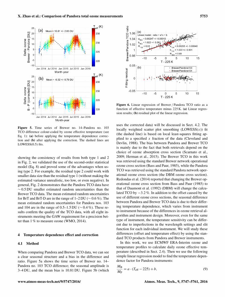
Figure 5. Time series of Brewer no. 14–Pandora no. 103TCO difference colour-coded by ozone effective temperature (seeEq. 1): (a) before applying the temperature dependence correc-tion and (b) after applying the correction. The dashed lines areLOWESS(0.5) fits.
showing the consistency of results from both type 1 and 2in Fig. 2, we validated the use of the second-order statisticalmodel (Eq. 8) and proved some of the advantages when us-ing type 2. For example, the residual type 2 could work withsmaller data size than the residual type 1 (without making theestimated variance unrealistic, too low, or even negative). Ingeneral, Fig. 2 demonstrates that the Pandora TCO data have∼ 0.5 DU smaller estimated random uncertainties than theBrewer TCO data. The mean estimated random uncertaintiesfor BrT and BrT-D are in the range of 1–2 DU (∼ 0.6 %). Themean estimated random uncertainties for Pandora nos. 103and 104 are in the range of 0.5–1.5 DU (∼ 0.4 %). These re-sults confirm the quality of the TCO data, with all eight in-struments meeting the GAW requirement for a precision bet-ter than 1 % to measure ozone (WMO, 2014).
4 Temperature dependence effect and correction
4.1 Method
When comparing Pandora and Brewer TCO data, we can seea clear seasonal structure and a bias in the difference andratio. Figure 5a shows the time series of Brewer no. 14–Pandora no. 103 TCO difference; the seasonal amplitude is3–4 DU, and the mean bias is 10.81 DU. Figure 5b (which
Figure 6. Linear regression of Brewer /Pandora TCO ratio as afunction of effective temperature minus 225 K. (a) Linear regres-sion results; (b) residual plot of the linear regression.
uses the corrected data) will be discussed in Sect. 4.2. Thelocally weighted scatter plot smoothing (LOWESS(x)) fit(the dashed line) is based on local least-squares fitting ap-plied to a specified x fraction of the data (Cleveland andDevlin, 1988). The bias between Pandora and Brewer TCOis mainly due to the fact that both retrievals depend on thechoice of ozone absorption cross section (Scarnato et al.,2009; Herman et al., 2015). The Brewer TCO in this workwas retrieved using the standard Brewer network operationalozone cross section (Bass and Paur, 1985), while the PandoraTCO was retrieved using the standard Pandora network oper-ational ozone cross section (the DBM ozone cross section).Redondas et al. (2014) reported that changing the Brewer op-erational ozone cross section from Bass and Paur (1985) tothat of Daumont et al. (1992) (DBM) will change the calcu-lated TCO by −3.2 %. In addition to the offset caused by theuse of different ozone cross sections, the seasonal differencebetween Pandora and Brewer TCO data is due to their differ-ing temperature dependence, which varies from instrumentto instrument because of the differences in ozone retrieval al-gorithm and instrument design. Moreover, even for the sametype of instrument, the temperature sensitivity can be differ-ent due to imperfections in the wavelength settings and slitfunction for each individual instrument. We will study thesedifferences (offset and temperature effect) by using the stan-dard TCO products from Pandora and Brewer instruments.
In this work, we use ECMWF ERA-Interim ozone andtemperature profiles to calculate daily ozone effective tem-perature (described in Sect. 2.4). Then we use the followingsimple linear regression model to find the temperature depen-dence factor for Pandora instruments:
5754 X. Zhao et al.: Comparison of Pandora total ozone measurements
where a is the temperature dependence factor for Pandora, bis the (systematic) multiplicative bias between Pandora andBrewer, and 225 refers to effective temperature of 225◦ K forozone cross sections used in the Pandora retrievals. Here, theMB and MP are TCO daily means measured by the Brewerand Pandora respectively. To increase the number of coin-cident data points, the MB dataset is formed by merging allmeasurements from the six Brewers (see Table 1). A success-fully merged MB data point has coincident measurementsfrom at least two Brewers, to avoid domination by a singleinstrument. The coincident time period of theMB andMP103datasets is from October 2013 to December 2015 with 272coincident days (points). Figure 6 shows the linear regres-sion results for Pandoras nos. 103 and 104. We found the“relative temperature dependence factor” (RTDF) for Pan-dora no. 103 to be 0.247± 0.013 % K−1 (from the term a
in Eq. 9), with a 2.2± 0.1 % multiplicative bias (from theterm b in Eq. 9). Although Pandora no. 104 only has mea-surements from January to April 2014 (53 coincident days),the linear regression still results in a similar temperature de-pendence factor (0.255± 0.040 % K−1) and the same bias asPandora no. 103. The correlation coefficients for those twolinear regressions are 0.91 and 0.89 respectively.
We applied the Pandora temperature dependence factors tothe Pandora TCO to remove its bias and seasonal differencerelative to Brewer TCO data. Similar to the correction func-tion used in Herman et al. (2015) for Pandora no. 34, we usedthe following function to correct Pandora TCO data:
Mcorr =MP · (a · (Teff− 225)+ b), (10)
where Mcorr is corrected Pandora TCO, and other terms areas defined for Eq. (9). For the Pandora no. 103 dataset, thisbecomes
where MP103 is the TCO data from Pandora no. 103. Thetemperature dependence factor (0.247± 0.013 % K−1) andthe multiplicative bias (1.022) are found in Fig. 6. The sameregression model and method give a 0.255± 0.040 % K−1
temperature dependence factor with a 2 % multiplicative biasto Pandora no. 104, and hence
where MP104 is the Pandora no. 104 TCO. For comparison,Herman et al. (2015) derived the correction function for Pan-dora no. 34 as
Mcorr =MP34 · (0.00333 · (Teff− 225)+ 1) , (13)
where the 0.00333 (0.333 % K−1) is the temperature depen-dence factor for Pandora no. 34. Note that this value was de-termined by applying retrievals using ozone cross sectionsfrom 215 to 240 K and then obtaining a linear fit to the per-cent change (Herman et al., 2015). However in this work, the
Figure 7. Pandora relative temperature dependence factors derivedfrom 13 sensitivity tests (shown in Table 3). (a) RTDFs, (b) multi-plicative biases, (c) correlation coefficients (R), and (d) number ofdata points in sensitivity tests. The error bars show the 95 % confi-dence bounds.
factors for Pandora nos. 103 and 104 were found by statis-tical analysis (comparison) of the Pandora and Brewer TCOdatasets. Thus our temperature dependence factor combinesthe temperature sensitivity from both Pandora and Brewer in-struments, and describes the relative temperature sensitivitybetween the Pandora and Brewer standard TCO products. Wecall it a “relative temperature dependence factor” (RTDF),while that from Herman et al. (2015) is an absolute tem-perature dependence factor (ATDF). Although the RTDF isa non-linear combination of ATDF from both Pandora andBrewer (note that the Pandora used an ozone cross sectionat an effective temperature of 225 K, while the Brewer usedthat at 223.8 K), we can still make a simple linear estima-tion of the RTDF from reported ATDFs. In fact, the reportedATDF for Pandora no. 34 (0.333 % K−1; Herman et al., 2015)minus the reported ATDF for Brewer nos. 8 and 14 (0.07and 0.094 % K−1; Kerr et al., 1988; Kerr, 2002) gives rel-ative numbers (0.26 and 0.24 % K−1) that are close to ourmodel-calculated RTDF (∼ 0.25 % K−1). In our correctionfunctions (Eqs. 11–12), we have a constant b term of 1.022given 0.001 uncertainty, which indicates a multiplicative biasof ∼ 2 % (not caused by the temperature effect) between thePandora and Brewer instruments due to their different selec-tion of ozone cross sections.
Merging data from all six Brewers could lead to variationof the Brewer temperature dependence, so we performed sen-sitivity tests on the dataset. Table 3 summarizes the tests;the combined Brewer data are merged from all availableBrewer data during the data period indicated in the table.Figure 7 shows the RTDFs, multiplicative bias, correlationcoefficient, and number of data points for the 13 sensitivitytests. Tests 1 and 2 are the results adapted from Fig. 6. Due
to the small data size, the RTDF for test 2 has larger errorbars than test 1. Test 3 shows Pandora no. 103 RTDF usingcombined Brewer data for the same time period as Pandorano. 104. Pandora no. 103 has a measurement gap from Au-gust to December 2014 due to instrument failure (see Fig. 1);hence, tests 4 and 5 use combined Brewer data for 2013–2014 (∼ 1-year coverage, before the instrument failure ofPandora no. 103) and 2015 (1-year coverage, after Pandorano. 103 was repaired) separately. Brewer no. 191 was oneof the most reliable Brewer instruments during the compar-ison period. Thus tests 6–8 use only Brewer no. 191 data;test 6 uses all available data (2013–2015), test 7 uses only2013–2014 data (before the instrument failure of Pandorano. 103), and test 8 uses 2015 data (after Pandora no. 103 wasrepaired). Tests 9–13 use individual Brewer data (all avail-able data for each individual Brewer). For the 13 tests, theRTDFs (see Fig. 7a) are in the range of 0.24–2.9 %, and themultiplicative biases (see Fig. 7b) are in the range of 1.7–2.5 %. The correlation coefficients (see Fig. 7c) for most testsare above 0.8. In general, the RTDFs found for the Pandorainstruments are stable when derived from combined Brewerdata or reliable individual Brewer data. For this 2-year dataperiod, the derived RTDFs from BrT-D instruments are lower(0.241–0.246 % K−1) than the ones from BrT instruments(0.262–0.290 % K−1). However, with the large uncertaintieson the estimated RTDFs and the bias, we could not concludewhether this is due to the different instrument designs or asampling issue.
5 Results
5.1 Pandora TCO correction
As an example, Fig. 5 shows the time series of Brewerno. 14–Pandora no. 103 TCO differences, before and afterapplying the Pandora correction (Eq. 11). A clear seasonalsignal is seen due to the variation of Teff before we apply
Figure 8. Scatter plots of Pandora no. 103 vs. Brewer no. 14 TCO,colour-coded by ozone effective temperature: (a) before applyingthe correction and (b) after applying the correction. The red lineis a simple linear fit, the green line is the linear fit weighted bythe calculated standard uncertainty from Pandora and Brewer TCOdata, the blue line is the linear fit with intercept set to 0, and theblack line is the one-to-one line.
the temperature dependence correction (see Fig. 5a). Figure 8shows scatter plots of Pandora no. 103 versus Brewer no. 14TCO. In Fig. 8a, the linear regression (green line, weightedaccounting for uncertainties from both measurements; Yorket al., 2004) between Pandora no. 103 and Brewer no. 14gives a slope of 1.023, an offset of −18.486 DU, and strongcorrelation (R = 0.9954). Forcing the intercept to 0 gives a
5756 X. Zhao et al.: Comparison of Pandora total ozone measurements
Figure 9. Effective ozone temperature: (a) Teff calculated usingECMWF ERA-Interim data (18:00 UTC over Toronto) and NASAclimatology data (monthly mean for 40–50◦ N), and (b) the differ-ence between these two.
slope of 0.969, indicating −3.1 % mean bias. This is consis-tent with the work of Redondas et al. (2014), which showedthat changing the Brewer ozone cross section from Bassand Paur to DBM changed the Brewer TCO by −3.2 %.By colour coding the scatter points, it is obvious that thisnon-ideal slope and offset are related to Teff . After applyingthe correction, the seasonal Brewer–Pandora difference dis-appears as seen in Fig. 5b, and the linear regression (greenline) gives a slope of 1.008, an offset of −2.678 DU, and animproved correlation (R = 0.9982) (see Fig. 8b). Linear fit-ting with zero intercept gives a slope of 1.001, indicating thatthe correction improves the mean bias between Pandora andBrewer TCO from −3.1 to 0.1 %.
To calculate the effective temperature, we use daily tem-perature and ozone profiles from ECMWF ERA-Interim dataat 18:00 UTC for Toronto, but Herman et al. (2015) usedmonthly averaged temperature and ozone climatology data(interpolating the climatological ozone profile to the ob-served TCO in order to capture day-to-day variability; seeftp://toms.gsfc.nasa.gov/pub/ML_climatology) for latitudesof 30–40 and 40–50◦ N to form an average suitable for Boul-der (40◦ N). To understand the difference due to the selectionof Teff, we adapted the climatology data used in Herman etal. (2015) and used the data from 40 to 50◦ N to calculateeffective ozone temperature for Toronto (44◦ N). Figure 9shows the comparison between the ECMWF daily Teff andthe NASA monthly climatology Teff. A sudden cooling eventhappened at Toronto on 29–30 January 2014, for which thedifference between the daily and monthly Teff was −10 K.Figure 10 shows the time series of TCO difference (com-bined Brewer–Pandora no. 103) before and after applying thetemperature dependence correction using both the monthlyclimatology Teff and daily Teff. Because the monthly clima-tology Teff does not reflect the low temperature during thosetwo days, the correction function (see Eq. 11) overcompen-sated for the temperature effect (the minimum delta ozonevalue on 29 January changed from −8 DU in Fig. 10a to−14 DU in Fig. 10b). The low-temperature event was cap-
Figure 10. Time series of combined Brewer–Pandora no. 103 TCOdifference colour-coded by ozone effective temperature: (a) beforeapplying the temperature dependence correction, (b) after applyingthe correction using NASA monthly climatology Teff, and (c) afterapplying the correction using ECMWF EAR-Interim daily Teff. Thesudden cooling event on 29–30 January 2014 is marked by a blackbox. The dashed lines are LOWESS(0.5) fits.
tured by the daily Teff; thus the compensation from the tem-perature effect was reasonably small when using ECMWFdaily Teff (the minimum value was −7 DU; see Fig. 10c).In general, the ECMWF daily Teff can better capture someozone variation events that are associated with rapid temper-ature changes.
Figure 11 shows time series of the monthly average TCOdifference in percentage before and after applying the tem-perature dependence correction for eight pairs of instru-ments (six individual Brewers vs. Pandora no. 103, com-bined Brewer vs. Pandora no. 103, and combined Brewervs. Pandora no. 104). Figure 11a shows that both Pandoranos. 103 and 104 have similar offsets relative to the Brewersbefore applying the correction to Pandora data. In addition,the seasonal variations are consistent when comparing Pan-dora no. 103 to six individual Brewers (see Fig. 11a). After
X. Zhao et al.: Comparison of Pandora total ozone measurements 5757
Figure 11. Monthly mean time series of the(Brewer−Pandora) /Brewer % TCO difference: (a) beforeapplying the Pandora temperature dependence correction and(b) after applying the correction. The shaded regions represent 1σuncertainty.
applying the TCO corrections (Fig. 11b), the seasonal differ-ences decreased from±1.02 to±0.25 % for Pandora no. 103and from ±0.40 to ±0.25 % for Pandora no. 104, as did theoffset which decreased from 2.92 to −0.04 % for Pandorano. 103 and from 2.11 to −0.01 % for Pandora no. 104. The1σ uncertainty in Fig. 11b shows that, statistically, the cor-rected Pandora datasets have no significant seasonal differ-ences or offsets compared to the Brewer datasets.
5.1.1 Comparison with OMI
To further validate the temperature dependence correctionfor the Pandora data, we used OMI ozone data (versionOMTO3e). Pandora data are averaged within ±10 min ofOMI overpass times. In Fig. 12, scatter plots of OMI vs.Pandora TCO are shown in panels a and b; OMI vs. cor-rected Pandora TCO (using Eqs. 11 and 12 with the correc-tion functions found from our statistical model) is shown inpanels c and d; and OMI vs. corrected Pandora TCO (us-ing Eq. 13 with the correction function from Herman et al.,2015) is shown in panels e and f. All the Pandora TCO cor-rections shown in Fig. 12 used the same Teff calculated withthe ECMWF ERA-Interim daily ozone data.
Figure 12a and c show that, after applying the TCO cor-rection (Eq. 11) to Pandora no. 103, the slope of the lin-ear regression improved from 0.987 to 0.990, the offset im-proved from 14.84 to −3.59 DU, the correlation coefficientimproved from 0.987 to 0.991, and the mean bias between
Figure 12. Scatter plots of OMI TCO vs. Pandora TCO for (a) Pan-dora no. 103 without TCO correction, (b) Pandora no. 104 withoutTCO correction, (c) Pandora no. 103 with correction using Eq. (11),(d) Pandora no. 104 with correction using Eq. (12), (e) Pandorano. 103 with correction using Eq. (13), and (f) Pandora no. 104 withcorrection using Eq. (13).
OMI and Pandora improved from 3.1 to 0.02 %. Similarimprovement is seen in the comparison between Pandorano. 104 and OMI (see Fig. 12b and d), although the size ofthe coincident measurement dataset is smaller, with the meanbias improving from 1.5 to −0.6 %. In addition, Fig. 12eand f show that, by using the correction function from Her-man et al. (2015), the comparisons also improve, although1.9 % (1.4 %) bias remains for Pandora no. 103 (no. 104) (in-dicated by the slop of linear fit with force the intercept to 0;see the green lines in Fig. 12). Note that the ATDF in Hermanet al. (2015) is only 0.08 % K−1 higher than our RTDF.
Figure 13a and b shows the monthly mean time series ofthe OMI–Pandora TCO percentage difference, before andafter applying the three correction functions. All three cor-rection models reduced the difference between Pandora andOMI. Our relative correction model (Eqs. 11 and 12) reducesthe seasonal difference (indicated by the δ of the percent-age monthly delta ozone) between Pandora no. 103 and OMIfrom ±1.68 to ±1.00 %, with the mean bias decreasing from2.65 to −0.19 % (the mean of the percentage monthly deltaozone). Pandora no. 104 has a similar improvement. The ab-solute correction model (Eq. 13) reduces the seasonal dif-ference between Pandora no. 103 and OMI to 0.87 %, withthe mean bias decreased to 1.71 %. The reduction in the
5758 X. Zhao et al.: Comparison of Pandora total ozone measurements
Figure 13. Monthly mean time series of the(OMI−Pandora) /OMI % TCO difference: (a) before applying thecorrection, (b) after applying the correction using Eqs. (11)–(13),and (c) the difference between the corrections. The shaded regionsrepresent the 1σ uncertainty.
mean bias between Pandora and OMI is better for the relativecorrection model. This result (−0.19± 1.00 % mean bias)is consistent with Balis et al. (2007), who showed that theglobal average difference between OMI–TOMS and Brewerinstruments is within 0.6 %, and that the difference in the40–50◦ N band (Toronto is at 44◦ N) is close to 0 (see theirFig. 1).
Balis et al. (2007) reported that the time series of glob-ally averaged differences between OMI–TOMS and Brewerinstruments shows almost no annual variation, and the OMI–TOMS data theoretically have no temperature dependence(McPeters and Labow, 1996; Bhartia and Wellemeyer, 2002).By using our relative correction, the corrected Pandora TCOshould have similar performance to the Brewer TCO. Fig-ure 13c shows the difference between the absolute correctionmethod and the relative correction method. Although bothmethods removed some of the seasonal signal (reduced from
1.68 to 1.00 % for the relative correction and to 0.87 % forthe absolute correction), Fig. 13c shows that there is stilla weak seasonal signal residual (0.39 %) left between thesetwo methods.
6 Stray-light effect
It is well known that direct-sun UV spectrometers are af-fected by stray light when the solar zenith angle (SZA) istoo large. In general, when the ozone AMF is larger than3 (SZA> 70◦), the retrieved TCO will show an unrealis-tic decrease with increasing SZA (thus this effect is alsoknown as the air mass dependence effect). In general, thestray light from longer wavelengths results in overestimationof the UV signal at short wavelengths and makes the mea-sured UV signal in that part of the spectrum less sensitiveto TCO. The double Brewer spectrometer was introduced in1992, which uses two spectrometers in series to reduce thestray light (Bais et al., 1996; Wardle et al., 1996; Fioletov etal., 2000). The BrT-D has the advantage of very low internalstray-light fraction (10−7, stray-light signal divided by totalsignal) compared to BrT (10−5) in the 300–330 nm spectralrange (Fioletov et al., 2000; Tzortziou et al., 2012). For Pan-dora instruments, a UV340 filter is used to remove most ofthe stray light that originates from wavelengths longer than380 nm (Herman et al., 2015). A typical UV340 filter has asmall leakage (5 %) at ∼ 720 nm, which misses the detectorand hits the internal baffles. Further stray-light correction isdone by subtracting the signal of pixels corresponding to 280to 285 nm (which contain almost zero direct illumination)from the rest of the spectrum. However, a very small (butunknown) amount of this stray light may scatter onto the de-tector (Herman et al., 2015). Tzortziou et al. (2012) tested thestray-light effect for Pandora no. 34 and Brewer no. 171 andconcluded that the Pandora stray-light fraction (∼ 10−5) wascomparable to the single Brewer. Pandora ozone retrievalsare accurate up to a slant column between 1400 and 1500 DUor 70 and 80◦ SZA, depending on the TCO amount (Hermanet al., 2015).
In this work, to assess the air mass dependence, we com-pared Brewer TCO to the corrected Pandora TCO data. Fig-ure 14 shows an example of the Brewer /Pandora ratio as afunction of ozone AMF (reported value in Brewer data) be-fore and after applying the TCO correction (Eq. 11), withthe data points grouped by effective temperature. Before ap-plying the correction (Fig. 14a), the linear fits show con-sistently low (−0.1 to 0.5 %) relative AMF dependence be-tween Brewer and Pandora (defined as the slope of the linearfit) for each Teff group. However, the linear fit to the wholedataset (all effective temperatures, black line) shows that therelative AMF dependence is −0.007. Figure 14b shows thatthe correction changed the slope of the black line to −0.001;removing the temperature effect for the Pandora dataset thusreduces the relative AMF dependence from −0.7 to −0.1 %.
X. Zhao et al.: Comparison of Pandora total ozone measurements 5759
Figure 14. Brewer no. 14 /Pandora no. 103 TCO ratio vs. ozone airmass factor: (a) before and (b) after applying the Pandora temper-ature dependence correction. The points are grouped by effectivetemperature (from 215 to 240 K, in 5 K bins), and the linear fits foreach group are colour-coded. The black line and linear fit are for thewhole dataset.
Figure 15. Percentage difference between Pandoras (nos. 103and 104) and Brewers (grouped as BrT and BrT-D) as a functionof ozone air mass factor. On each box, the central mark is the me-dian, the edges of the box are the 25th and 75th percentiles, andthe whiskers extend to the most extreme data points not consideredoutliers.
To characterize only the air mass dependence, we thereforeremoved the temperature dependence effect from the Pan-dora dataset.
To show how the different instrument designs affectthe stray-light performance, we merged the six Brewerdatasets into two groups (BrT and BrT-D) to compare
with the corrected Pandora data. Figure 15 shows the(Brewer−Pandora) /Brewer percentage difference as afunction of ozone AMF. In Sects. 3 and 4, the TCO datawith ozone AMF> 3 were discarded. The purpose of this fil-ter was to ensure that only the best direct-sun measurements(with low air mass dependence) from both instruments wereused. However, to study the instrument performance for largeAMFs, and also to characterize the performance of Brewerand Pandora instruments, we changed the AMF thresholdfrom 3 to 6. Figure 15 indicates that Pandora, BrT, and BrT-D instruments have similar air mass dependence for ozoneAMF< 3 (∼ 71◦ SZA), consistent with the result reportedby Tzortziou et al. (2012). Pandora and BrT-D have similarAMF dependence up to ozone AMF of 5.5–6 (80.6–81.6◦
SZA), but Pandora and BrT diverge above AMF of 3–4 (71–76◦ SZA). In general, these results indicate the Pandora andBrT-D instruments have very good stray-light control.
7 Conclusions
The instrument random uncertainty, TCO temperature de-pendence, and ozone air mass dependence have been de-termined using two Pandora and six Brewer instruments. Ingeneral, Pandora and Brewer instruments both have very lowrandom uncertainty (< 2 DU) in the total column ozone mea-surements, with that for Pandora being ∼ 0.5 DU lower thanBrewer. This indicates that Pandora instruments could pro-vide more precise measurements than the Brewer for thestudy of small-scale (temporal and magnitude) atmosphericchanges. This work confirms the quality of the TCO data,with all eight instruments meeting the GAW requirementfor a precision better than 1 % (WMO, 2014); however, theBrewer instruments have smaller ozone temperature depen-dence than the Pandoras.
By using the ECMWF ERA-Interim and Brewer ozonedata in the statistical method, we successfully correctedthe Pandora TCO to decrease its temperature depen-dence. We found relative temperature dependence factors of0.247 % K−1 for Pandora no. 103 and 0.255 % K−1 for Pan-dora no. 104 against the Brewer instruments. This relativetemperature dependence factor is comparable to the abso-lute temperature dependence factors previously found forPandora (0.333 % K−1, by applying retrievals with differ-ent ozone cross sections, Herman et al., 2015) and Brewers(0.07–0.094 % K−1; Kerr et al., 1988; Kerr, 2002). In addi-tion, a 2 % multiplicative bias was found between the Pan-dora and Brewer standard TCO products, which is due tothe different ozone cross sections used in the retrievals. Af-ter applying the corrections, the annual seasonal differencebetween Pandora and Brewer instruments decreased from±1.02 to ±0.25 %, and the mean bias decreased from 2.92to 0.04 %. In addition to using model ozone data (ECMWFERA-Interim for our case) to calculate the effective ozonetemperature, it could also be estimated from Brewer or Pan-
5760 X. Zhao et al.: Comparison of Pandora total ozone measurements
dora measurements (Kerr, 2002; Tiefengraber et al., 2016),albeit at a cost of decreased TCO measurement precision. Aneffective ozone temperature algorithm is under developmentfor the Pandora. The future operational Pandora ozone re-trieval algorithm will use this derived effective ozone temper-ature to minimize the temperature dependence of the ozoneproduct (Tiefengraber et al., 2016).
This study confirmed that the Pandora and Brewer TCOdata have negligible air mass dependence when the ozoneAMF< 3. The Pandora and BrT instruments have similar airmass dependence (relative air mass dependence <± 0.1 %)up to 71◦ SZA (AMF< 3); the Pandora and BrT-D instru-ments have very good stray-light control, and their AMF de-pendence is comparably low up to 81.6◦ SZA (within 1 % upto AMF= 5.5 and within 1.5 % up to AMF= 6).
8 Data availability
Data from the BrT, BrT-D, and Pandora instrumentsare available through Environment and Climate ChangeCanada (contact Vitali Fioletov, [email protected]).The final version of the Brewer data is (or will be)available from the World Ozone and UV Data Centre(doi:10.14287/10000001). OMTO3e data are available fromthe GES DISC: doi:10.5067/Aura/OMI/DATA3002 (GESDISC, 2004). Any additional data may be obtained from Xi-aoyi Zhao ([email protected]).
Acknowledgements. X. Zhao was partially supported by theNSERC CREATE Training Program in Arctic AtmosphericScience. We thank ECMWF for providing the ERA-Interim modeldata and the NASA OMI ozone retrieval team for providing theOMTO3e data.
Edited by: M. Van RoozendaelReviewed by: three anonymous referees
References
Bais, A., Zerefos, C., and McElroy, C.: Solar UVB measurementswith the double-and single-monochromator Brewer ozone spec-trophotometers, Geophys. Res. Lett., 23, 833–836, 1996.
Balis, D., Kroon, M., Koukouli, M., Brinksma, E., Labow, G.,Veefkind, J., and McPeters, R.: Validation of Ozone MonitoringInstrument total ozone column measurements using Brewer andDobson spectrophotometer ground-based observations, J. Geo-phys. Res., 112, D24S46, doi:10.1029/2007JD008796, 2007.
Bass, A. and Paur, R.: The ultraviolet cross-sections of ozone: I. Themeasurements, in: Atmospheric Ozone, Springer, the Nether-lands, 606–610, 1985.
Bhartia, P. and Wellemeyer, C.: OMI TOMS-V8 Total O3 algorithm,algorithm theoretical baseline document: OMI ozone products,NASA Goddard Space Flight Cent, Greenbelt, Md, 2002.
Bhartia, P.: OMI/Aura TOMS-Like Ozone and Radiative CloudFraction Daily L3 Global 0.25×0.25 deg, NASA Goddard SpaceFlight Center, doi:10.5067/Aura/OMI/DATA3002, 2012.
Brion, J., Chakir, A., Daumont, D., Malicet, J., and Parisse,C.: High-resolution laboratory absorption cross section ofO3, Temperature effect, Chem. Phys. Lett., 213, 610–612,doi:10.1016/0009-2614(93)89169-I, 1993.
Brion, J., Chakir, A., Charbonnier, J., Daumont, D., Parisse, C.,and Malicet, J.: Absorption Spectra Measurements for the OzoneMolecule in the 350–830 nm Region, J. Atmos. Chem., 30, 291–299, doi:10.1023/a:1006036924364, 1998.
Cleveland, W. S. and Devlin, S. J.: Locally weighted regression:an approach to regression analysis by local fitting, J. Am. Stat.Assoc., 83, 596–610, 1988.
Daumont, D., Brion, J., Charbonnier, J., and Malicet, J.: Ozone UVspectroscopy I: Absorption cross-sections at room temperature,J. Atmos. Chem., 15, 145–155, doi:10.1007/bf00053756, 1992.
Dee, D. P., Uppala, S. M., Simmons, A. J., Berrisford, P., Poli,P., Kobayashi, S., Andrae, U., Balmaseda, M. A., Balsamo, G.,Bauer, P., Bechtold, P., Beljaars, A. C. M., van de Berg, L., Bid-lot, J., Bormann, N., Delsol, C., Dragani, R., Fuentes, M., Geer,A. J., Haimberger, L., Healy, S. B., Hersbach, H., Hólm, E. V.,Isaksen, L., Kållberg, P., Köhler, M., Matricardi, M., McNally,A. P., Monge-Sanz, B. M., Morcrette, J. J., Park, B. K., Peubey,C., de Rosnay, P., Tavolato, C., Thépaut, J. N., and Vitart, F.: TheERA-Interim reanalysis: configuration and performance of thedata assimilation system, Q. J. Roy. Meteor. Soc., 137, 553–597,doi:10.1002/qj.828, 2011.
Dobson, G. M. B.: Exploring the atmosphere, 2nd Edn., ClarendonPress, Oxford, XV, 209 pp., 1968.
Dunn, G.: Statistical evaluation of measurement errors: Design andanalysis of reliability studies, John Wiley & Sons, 2009.
Farman, J. C., Gardiner, B. G., and Shanklin, J. D.: Large losses oftotal ozone in Antarctica reveal seasonal ClOx /NOx interaction,Nature, 315, 207–210, 1985.
Fioletov, V., Kerr, J., Wardle, D., and Wu, E.: Correction of straylight for the Brewer single monochromator, Proceedings of theQuadrennial Ozone Symposium, Sapporo, Japan, 3–8 July 2000,369–370, 2000.
Fioletov, V., Kerr, J., McElroy, C., Wardle, D., Savastiouk, V., andGrajnar, T.: The Brewer reference triad, Geophys. Res. Lett., 32,L20805, doi:10.1029/2005GL024244, 2005.
Fioletov, V., Tarasick, D., and Petropavlovskikh, I.: Esti-mating ozone variability and instrument uncertainties fromSBUV (/2), ozonesonde, Umkehr, and SAGE II measure-ments: Short-term variations, J. Geophys. Res., 111, D02305,doi:10.1029/2005jd006340, 2006.
GES DISC: OMTO3e: OMI/Aura TOMS-Like Ozone and Ra-diative Cloud Fraction L3 1 day 0.25◦× 0.25◦ V3, NASAGoddard Earth Sciences (GES) Data and Information ServicesCenter (DISC), doi:10.5067/Aura/OMI/DATA3002 (last access:November 2016), 2004.
Grubbs, F. E.: On estimating precision of measuring instrumentsand product variability, J. Am. Stat. Assoc., 43, 243–264, 1948.
Herman, J., Cede, A., Spinei, E., Mount, G., Tzortziou, M., andAbuhassan, N.: NO2 column amounts from ground-based Pan-dora and MFDOAS spectrometers using the direct-Sun DOAStechnique: Intercomparisons and application to OMI validation,
X. Zhao et al.: Comparison of Pandora total ozone measurements 5761
J. Geophys. Res., 114, D13307, doi:10.1029/2009JD011848,2009.
Herman, J., Evans, R., Cede, A., Abuhassan, N., Petropavlovskikh,I., and McConville, G.: Comparison of ozone retrievals fromthe Pandora spectrometer system and Dobson spectrophotome-ter in Boulder, Colorado, Atmos. Meas. Tech., 8, 3407–3418,doi:10.5194/amt-8-3407-2015, 2015.
Kerr, J.: New methodology for deriving total ozone andother atmospheric variables from Brewer spectropho-tometer direct sun spectra, J. Geophys. Res., 107, 4731,doi:10.1029/2001JD001227, 2002.
Kerr, J., McElroy, C., and Olafson, R.: Measurements of ozone withthe Brewer ozone spectrophotometer, Proceedings of Quadren-nial International Ozone Symposium, 4–9 August 1980, Boulder,CO, 74–79, 1980.
Kerr, J., Asbridge, I., and Evans, W.: Intercomparison of totalozone measured by the Brewer and Dobson spectrophotometersat Toronto, J. Geophys. Res., 93, 11129–11140, 1988.
Kerr, J., McElroy, C., and Wardle, D.: The Brewer instrumentcalibration center 1984–1996, Proceedings of the QuadrennialOzone Symposium, 12–21 September 1996, L’Aquila, Italy,915–918, 1996.
Kroon, M., Veefkind, J. P., Sneep, M., McPeters, R. D., Bhar-tia, P. K., and Levelt, P. F.: Comparing OMI–TOMS and OMI–DOAS total ozone column data, J. Geophys. Res., 113, D16S28,doi:10.1029/2007jd008798, 2008.
Levelt, P. F., Hilsenrath, E., Leppelmeier, G. W., Van den Oord, G.H., Bhartia, P. K., Tamminen, J., De Haan, J. F., and Veefkind, J.P.: Science objectives of the ozone monitoring instrument, IEEET. Geosci. Remote, 44, 1199–1208, 2006.
McPeters, R. D. and Labow, G. J.: An assessment of the accuracy of14.5 years of Nimbus 7 TOMS version 7 ozone data by compar-ison with the Dobson network, Geophys. Res. Lett., 23, 3695–3698, doi:10.1029/96gl03539, 1996.
Noxon, J.: Nitrogen dioxide in the stratosphere and tropospheremeasured by ground-based absorption spectroscopy, Science,189, 547–549, 1975.
Platt, U. and Stutz, J.: Differential Optical Absorption Spec-troscopy: Principles and Applications, Springer, Berlin, 597 pp.,2008.
Ramaswamy, V., Schwarzkopf, M. D., and Shine, K. P.: Radiativeforcing of climate from halocarbon-induced global stratosphericozone loss, Nature, 355, 810–812, 1992.
Redondas, A., Evans, R., Stuebi, R., Köhler, U., and Weber, M.:Evaluation of the use of five laboratory-determined ozone ab-sorption cross sections in Brewer and Dobson retrieval algo-rithms, Atmos. Chem. Phys., 14, 1635–1648, doi:10.5194/acp-14-1635-2014, 2014.
Roscoe, H. K., Van Roozendael, M., Fayt, C., du Piesanie, A.,Abuhassan, N., Adams, C., Akrami, M., Cede, A., Chong, J.,Clémer, K., Friess, U., Gil Ojeda, M., Goutail, F., Graves, R.,Griesfeller, A., Grossmann, K., Hemerijckx, G., Hendrick, F.,Herman, J., Hermans, C., Irie, H., Johnston, P. V., Kanaya, Y.,Kreher, K., Leigh, R., Merlaud, A., Mount, G. H., Navarro, M.,Oetjen, H., Pazmino, A., Perez-Camacho, M., Peters, E., Pinardi,G., Puentedura, O., Richter, A., Schönhardt, A., Shaiganfar, R.,Spinei, E., Strong, K., Takashima, H., Vlemmix, T., Vrekoussis,
M., Wagner, T., Wittrock, F., Yela, M., Yilmaz, S., Boersma, F.,Hains, J., Kroon, M., Piters, A., and Kim, Y. J.: Intercomparisonof slant column measurements of NO2 and O4 by MAX-DOASand zenith-sky UV and visible spectrometers, Atmos. Meas.Tech., 3, 1629–1646, doi:10.5194/amt-3-1629-2010, 2010.
Scarnato, B., Staehelin, J., Peter, T., Gröbner, J., and Stübi, R.:Temperature and slant path effects in Dobson and Brewertotal ozone measurements, J. Geophys. Res., 114, D24303,doi:10.1029/2009JD012349, 2009.
Solomon, S., Garcia, R. R., Rowland, F. S., and Wuebbles, D. J.: Onthe depletion of Antarctic ozone, Nature, 321, 755–758, 1986.
Solomon, S., Schmeltekopf, A., and Sanders, R.: On the interpreta-tion of zenith sky absorption measurements, J. Geophys. Res., 2,8311–8319, 1987.
Stolarski, R. S., Krueger, A. J., Schoeberl, M. R., McPeters, R. D.,Newman, P. A., and Alpert, J. C.: Nimbus 7 satellite measure-ments of the springtime Antarctic ozone decrease, Nature, 322,808–811, doi:10.1038/322808a0, 1986.
Stolarski, R. S., Bloomfield, P., McPeters, R. D., and Herman, J. R.:Total Ozone trends deduced from Nimbus 7 Toms data, Geophys.Res. Lett., 18, 1015–1018, doi:10.1029/91gl01302, 1991.
Tiefengraber, M., Cede, A., and Cede, K.: ESA Ground-BasedAir-Quality Spectrometer Validation Network and UncertaintiesStudy: Report on Feasibility to Retrieve Trace Gases other thanO3 and NO2 with Pandora, LuftBlick, 32, 17–19, 2016.
Toohey, M. and Strong, K.: Estimating biases and error variancesthrough the comparison of coincident satellite measurements, J.Geophys. Res., 112, D13306, doi:10.1029/2006JD008192, 2007.
Tzortziou, M., Herman, J. R., Cede, A., and Abuhassan, N.: Highprecision, absolute total column ozone measurements from thePandora spectrometer system: Comparisons with data from aBrewer double monochromator and Aura OMI, J. Geophys. Res.,117, D16303, doi:10.1029/2012JD017814, 2012.
Van Roozendael, M., Peeters, P., Roscoe, H., De Backer, H., Jones,A., Bartlett, L., Vaughan, G., Goutail, F., Pommereau, J.-P., andKyro, E.: Validation of ground-based visible measurements oftotal ozone by comparison with Dobson and Brewer spectropho-tometers, J. Atmos. Chem., 29, 55–83, 1998.
Veefkind, J. P., Haan, J. F. d., Brinksma, E. J., Kroon, M., andLevelt, P. F.: Total ozone from the ozone monitoring instrument(OMI) using the DOAS technique, IEEE T. Geosci. Remote., 44,1239–1244, doi:10.1109/tgrs.2006.871204, 2006.
Wardle, D., McElroy, C., Kerr, J., Wu, E., and Lamb, K.: Labora-tory tests on the double Brewer spectrophotometer, Proceedingsof the Quadrennial Ozone Symposium, L’Aquila, Italy, 12–21September, 1996, 997–1000, 1996.
WMO: Scientific Assessment of Ozone Depletion: 2014, GlobalOzone Research and Monitoring Project-Report No. 55, 416,2014.
York, D., Evensen, N. M., Martınez, M. L., and Delgado, J. D. B.:Unified equations for the slope, intercept, and standard errors ofthe best straight line, Am. J. Phys., 72, 367–375, 2004.