Speed and Expertise in Stock Picking: Older, Slower, and Wiser?

Romain Boulland

ESSEC Business School

Chay Ornthanalai

University of Toronto

Kent L. Womack

University of Toronto

For helpful comments, we thank Daniel Bradley, Jonathan Clarke, Lily Fang, Jose Guedes, Heiko Jacobs, Jennifer Jordan, Ohad Kadan, Stefan Lewellen, Roger Loh, Jay Ritter, Maria Rotundo, Richard Thaler, David Veenman, and Frank Zhang. We especially thank Alok Kumar and Kelvin Law for providing us with data on analysts’ gender, and thank Lily Fang and Ayako Yasuda for providing us with Institutional Investor’s all-star analyst data. This paper has benefited from comments by conference and seminar participants at AFA 2017, EFA 2015, ESSEC, MIT-Asia 2015, NFA 2015, FMA 2015, NTU, HKUST, Singapore Management University, University Paris-Dauphine, University of Alberta, University of Arizona, University of Oklahoma, and University of Florida. Romain Boulland is at ESSEC Business School. Chay Ornthanalai is at the Rotman School of Management, University of Toronto. Kent Womack was affiliated with the Rotman School of Management, University of Toronto. We thank Valerie Zhang, Ching Tse Chen, Talha Irshad, and Yang (Karl) Qu for their excellent research assistance on this paper. Ornthanalai gratefully acknowledges financial support from the Social Science and Humanities Research Council (SSHRC). Please send correspondence to Chay Ornthanalai at 105 St. George Street, Toronto, ON, M5S 3E6, Canada; chay.ornthanalai@rotman.utoronto.ca. We are responsible for all inadequacies.

0

Speed and Expertise in Stock Picking: Older, Slower, and Wiser?

Abstract

There are significant differences among sell-side analysts in how frequently they revise recommendations. We show that much of this variation is an analyst-individual trait. Analysts who change their recommendations more slowly make recommendations that are more influential and generate better portfolio returns. Examining the sources of differing investment value, we find that recommendations of slower-revising analysts are more likely to “lead the pack,” and revised following corporate disclosures that are harder to assess by non-stock experts. Analysts tend to change recommendations less frequently as their career progresses; however, recommendation speed-style is the only robust predictor of their recommendation value.

1

1. Introduction“All of us would be better investors if we just made fewer decisions.”

–— Daniel Kahneman1

Two decades of academic research support the view that sell-side analysts play an

important role in collecting, digesting, and disseminating value-relevant market

knowledge to investors.2 As information processing agents who are surely monitored

by their own firms and their clients, these analysts have incentives to be accurate

and to predict the future corporate activities and stock prices of their target firms.

And, as documented in an important stream of the literature, analysts’ attention to

their own reputations and career concerns affect their decisions (Hong and Kubik,

2003; Clement and Tse, 2005; Hilary and Hsu, 2013).

This study examines speed as an important decision-making-process choice

of individual analysts. All else equal, one might hypothesize that reputation

would be enhanced by “getting there first,” i.e. beating industry competitors

by reacting quicker to new information. Even in more traditional information-

based investing, virtually all event-based trading rules are less profitable if

the decision maker’s reaction to the event is delayed. But there is another

side to the speed story. Warren Buffet’s famous line, “Wait for the fat pitch,”

is a decision maxim urging investors not to be in a hurry because there are

many investment opportunities, but not many good ones. There may also be

other cogent reasons for slower decision-making. If an analyst is really

talented, his previous recommendations will remain accurate longer. Thus, a

truly talented analyst should have less need to change them frequently.

Several factors could affect when analysts revise their recommendations.

1 Nobel laureate in economics, in Jason Zweig, “Do You Sabotage Yourself?” Money Magazine, May, 2001, p. 78.

2 For some evidences, see Womack (1996), Clement (1999), Barber et al. (2001), Frankel, Kothari and Weber (2006), and Fang and Yasuda (2009). For a survey, see Bradshaw (2011).

2

Intuitively, an analyst would change a stock recommendation when his

assessment of the stock value (V) sufficiently deviates from the current share

price (P). If the ratio of an analyst’s stock valuation to price (V/P) exceeds or

falls below a certain threshold, then a recommendation is triggered. Under

this framework, variations in the timing of recommendation changes can

come through four channels. The first is the arrival of new information that

alters an analyst’s assessment of the stock value (V). This new information

could be in the form of public news about the company (e.g., earnings

announcements) or news about the industry. Also, the information that

analysts acquire need not be publicly observable but arrive through private

channels such as their interaction with firm managers. The second channel for

which variations in the recommendation speed can arise is through the

publicly traded share price (P). For instance, a sudden stock price jump can

trigger a recommendation change which can occur with news arrival, as well

as in its absence. The third channel that can explain variations in

recommendation-change speed relates to the nature of a new

recommendation that the analyst is evaluating. This includes the magnitude

of recommendation changes that the analyst is contemplating, as well as the

current recommendation level.

Finally, the fourth channel that can explain variations in the

recommendation-speed is the analyst-person characteristic. This may be due

to the speed at which some analysts collect and absorb information, as well

as the difference in their valuation approaches (Kahneman, 2011). The speed

at which analysts revise their recommendations may also be a strategic

choice. As shown in Bernhardt, Wan and Xiao (2016), frictions in

recommendation revisions can arise through the threshold in the valuation-to-

3

price ratio (V/P) that an analyst requires to exceed or fall below before a new

recommendation is warranted. This “revision threshold” is likely to differ

across analysts.

In this paper, we show that variations in the speed at which analysts revise

their recommendations is substantially explained by the “speed-style” of

individual analysts. After, we analyze the investment value of the differing,

inherent, decision-speed styles employed by stock experts.

We introduce a methodology to identify an analyst’s propensity to update

his recommendations on the spectrum of fast to slow, relative to his

competitors covering a similar portfolio of firms. We denote this speed-style

as the “recommendation turnover,” representing how often the analyst

overturns his recommendation opinions. The method builds on a simple

Binomial test and accounts for firm characteristics that may influence the

revision frequency, and the number of stocks that the analyst covers. At the

beginning of each calendar year, we use detailed recommendation history up

until the end of the previous year to classify analysts into three

recommendation turnover groups: (1) Slow, (2) Average, (3) Fast. We repeat

this process yearly from 1996 to 2013. As a result, our method provides an

out-of-sample estimate of analysts’ recommendation decision-speed types

from 1996 to 2013. On average, we find that fast-turnover analysts change

their recommendations every 6 months, while slow-turnover analysts typically

change their recommendations every 20 months.

We provide strong evidence that much of the variation in the speed at

which analysts revise their recommendations is an inherent-individual trait.

We illustrate this by estimating a hazard rate model for the probability that

each recommendation will be revised in relation to analysts’ recommendation

4

speed-styles identified from the previous year. We control for a host of

observable signals that may trigger or delay recommendation revisions and

our modeling approach allows for unobserved heterogeneity across analysts

(i.e., private information) that may affect their revision speed. Estimation

results indicate that analysts’ past recommendation speed-style strongly

predicts the speed at which they will revise their next recommendations. The

economic magnitude is large. The model estimates imply that on any given

week, fast-turnover analysts are about 2 times more likely to revise their

recommendations relative to slow-turnover analysts.

We next examine the value of recommendations made by analysts with

different decision-speed styles. We find that recommendation changes made

by slow-turnover analysts significantly outperform recommendation changes

by fast-turnover analysts. The immediate stock market reaction to

recommendation changes of slow-turnover analysts is 46–76 basis points

greater in magnitude relative to those of fast-turnover analysts. This

magnitude difference is after controlling for various analyst and firm

characteristics that have been shown to affect the stock price reaction to

recommendation revisions.

We further confirm the differing investment values between fast- and slow-

turnover analysts by forming investable real-calendar-time portfolios in the

style of Barber et al. (2001). We form a portfolio that invests (and sells) one

dollar on the upgraded (downgraded) stock at the closing-day price after the

recommendation change. This method makes the strategy implementable for

ordinary investors. Overall, we find 5–10% differences in annualized portfolio

alphas from investing following slow- versus fast-turnover analysts’

recommendation changes.

5

We examine analyst characteristics that are associated with different

recommendation speed-styles. An important aspect we observe is that during

the course of a career, there is a strong tendency for all surviving analysts to

change their recommendations less frequently. In fact, results from the logit

model show that analysts’ career tenure, i.e., experience, is the most

significant determinant of their decision-speed style. Other aspects that are

highly associated with slower-revising analysts include their likelihood of

being awarded the All-star status by the Institutional Investor magazine and

the size of their brokerage house. These aforementioned characteristics,

however, do not explain the investment value of slower decision-speed style.

At this point, we reemphasize that our method of identifying analysts’

recommendation speed-style is an out-of-sample approach, and importantly,

the investment value identified through the speed-style classification

dominates those identified through other analysts’ ex-ante characteristics

such as their career tenure, All-star status, prior earnings forecasts precision,

and brokerage house size.

The above results beg the following important questions: Why are analysts

who make less-frequent recommendations better stock pickers? What do cues

they use? Obviously, it is difficult, if not impossible, to see into the mind of

these decision makers, but we do observe valuable clues. First, we find that

slower (faster) recommendation-revising analysts are more likely to lead

(follow) others in recommendation changes as measured by the leader-

follower ratio of Cooper, Day and Lewis (2001). In other words, slow-turnover

analysts tend to issue recommendations that “lead the pack” even though

they revise them less frequently. Second, we find that analysts with different

decision-speed styles take cues from different news types when updating

6

their recommendations. Recent studies find that analysts’ recommendations

are valuable because they help investors interpret the contents of corporate

disclosures.3 Motivated by these studies, we examine the value of fast- versus

slow-turnover analysts in facilitating the price discovery of corporate

disclosures.

We obtain a comprehensive news database from Capital IQ that provides a

very fine classification of news categories and uncover distinct patterns in the

type of news that fast- vs. slow-turnover analysts tend to follow. We find that

fast-revising analysts are likely to update their recommendations following

verifiable and less ambiguous corporate disclosures such as scheduled

earnings announcements, or security issuances (e.g., debt issuance). On the

other hand, analysts who revise their recommendations more slowly tend to

do so following corporate news with potentially ambiguous price impact such

as news about the product market competition, operation strategy,

management forecasts, and legal issues. These news announcements are

mostly unscheduled and tend to carry forward-looking information about their

underlying firm value, which we believe are harder to intepret by non-stock

experts. We further corroborate this finding by manually reading 2,052

recommendation reports downloaded from Investext and reach a similar

conclusion.

This paper contributes to the sell-side analyst literature by identifying the

decision speed-style of stock experts based on the recommendations they

change, and by considering the differing investment value implications

thereof. Our work relates to studies that estimate models for how analysts

make recommendation changes. For instance, Conrad et al. (2006) models

3 See for examples, Livnat and Zhang (2012), and Rubin, Segal, and Segal (2017).7

how analysts change recommendations after large stock movements and find

that they are “sticky” in one direction, with analysts more reluctant to

downgrade.

A recent study by Bernhardt, Wan and Xiao (2016), which estimates the

model for how an analyst revises recommendations is perhaps the closest to

ours. Their study finds that analysts strategically introduce frictions when

updating their recommendations to avoid frequent revisions, and as argued

by the authors, this is because customers would question the ability of an

analyst who repeatedly revises recommendations. Our study differs from

Bernhardt, Wan and Xiao (2016) on several aspects. Their study documents

frictions in the recommendation decision of a representative analyst in the

sell-side industry. We show that there are significant differences among

analysts in the degree of frictions they apply to their recommendations and

that this variation is an analyst characteristic. Importantly, our method is

designed to identify analysts who are predictably quicker (or slower) to revise

their recommendations in an out-of-sample fashion. This enables us to study

their differing investment-value implications and implement them in practice.

We also provide evidence that reputation concern influences analysts to make

less frequent recommendation changes. Specifically, we show characteristics

that are associated with the slower speed-style are those that reflect

positively on analysts’ reputation such as All-star status, employment at a top

brokerage (Hong and Kubik, 2003), and career longevity (Prendergast and

Stole, 1996).

Hobbs, Kovacs and Sharma (2012) find superior portfolio performance

formed following recommendations of faster-revising analysts, suggesting

that quantity trumps quality; a conclusion that differs from ours. However,

8

their study measures analysts’ recommendation frequency using only

recommendations that are revised within 12 months. This approach would

eliminate about half of recommendation changes from the sample because

the median time between revisions is 11.2 months. This implies that their

study focuses on analysts who are already in the faster-extreme of

recommendation speed-style, or on a subset of stocks that require frequent

recommendation changes.4

This paper is organized as follows. Section 2 describes the data and the

methodology we use to identify analysts’ decision-speed style. Section 3

provides evidence that the decision-speed style is an analyst individual trait.

Section 4 discusses the investment value of differing decision-speed styles.

Section 5 examines the sources behind superior value of slower

recommendation-speed style. Finally, Section 6 concludes.

2. Data and methodology

2.1. Data and filters

We obtain analyst recommendations and earnings forecasts data from I/B/E/S. We

restrict our attention to equity analysts that appear in both the detailed

recommendation and forecast I/B/E/S files from 1993 to 2013.5 This initial sample

contains 629,400 recommendations made by 14,242 unique analysts. Security

returns data and firm-level information are obtained from CRSP and COMPUSTAT,

respectively. We identify “star analysts” based on Institutional Investor’s annual

4 We reconcile the difference between our finding and their study in the Online Appendix.

5 Ljungqvist, Malloy, and Marston (2009) document a significant number of additions, deletions, and alterations between snapshots of the I/B/E/S recommendation history on different dates. According to Wharton Research Data Services, the data distributor of I/B/E/S, the issues have been corrected as of September 2007.

9

ranking of All-American team (see Fang and Yasuda, 2009, 2013).6 The gender of

analysts is identified using their full names collected from the Institutional Investor

magazine and verified against multiple sources (see Kumar, 2010; and Law, 2013).7

We apply various filters to the I/B/E/S recommendation data file. We require

that firms in our sample have records on the CRSP daily database and have

CRSP share code of 10 or 11. We remove 19,809 anonymous

recommendations in I/B/E/S since it is not possible to track which analysts

issue these recommendations. We require that an analyst issues at least one

forecast and one recommendation change on a given stock for the analyst-

stock pair to be in our sample. Each recommendation in the I/B/E/S database

is coded with the rating scale between 1 and 5, ranging from “strong buy” to

“strong sell”, respectively.8 We characterize each revision as an upgrade or

downgrade. We do not consider initiations and reiterations in our empirical

analysis.

Kadan et al. (2009) document a significant number of mechanical

recommendation changes due to the migration of a five-tier rating system to

a three-tier rating system in 2002 following the National Association of

Securities Dealers (NASD) Rule 2711. We follow the method described in Loh

and Stulz (2011) for identifying these mechanical recommendation changes

and remove them from the sample. Up to this point, our recommendation

change sample contains 204,874 observations over 20 years, where 92,341

are upgrades.

6 We thank Lily Fang and Ayako Yasuda for sharing with us their Institutional Investor’s analyst ranking data.

7 We thank Alok Kumar and Kelvin Law for providing us with data on analyst gender.

8 Some brokerage firms use a 3-tier rating system instead of a 5-tier rating system.10

We define a recommendation as outstanding according to Ljungqvist,

Malloy, and Marston (2009). We remove recommendations that have been

dropped by each broker using I/B/E/S Stopped File. We further remove stale

recommendations that have been neglected by analysts without being

officially dropped by their broker. If an analyst’s recommendation has been

outstanding for more than one year without a reiteration and if this analyst

also makes less than one earnings forecast per year on the stock, we consider

his outstanding recommendation to be stale. We find 54,226

recommendations to have been outstanding for more than one year, and we

classify 3,533 of them as stale.

For each recommendation revision, we calculate the time a

recommendation is in place defined as the number of days between the

current and prior recommendation revision. Our final sample contains

196,074 recommendation changes made by 8,185 distinct analysts, where

88,248 are upgrades.

2.2 Sample descriptive

We focus on analysts who actively issue recommendations during the period 1996–

2013. Although I/B/E/S recommendation file begins in 1993, we start our analysis in

1996 in order to allow analysts’ recommendation history file to sufficiently develop.

In each year from 1996 to 2013, we calculate various characteristics for

each analyst. The number of analysts in our sample is updated yearly. We

require that an analyst provides active recommendation coverage on at least

three stocks. We consider that an analyst has initiated an active coverage of a

stock if he has issued at least two recommendation changes on the firm. The

final sample consists of 4,563 unique analysts who provide active

11

recommendation coverage during 1996–2013, resulting in 25,678 analyst-

year observations.

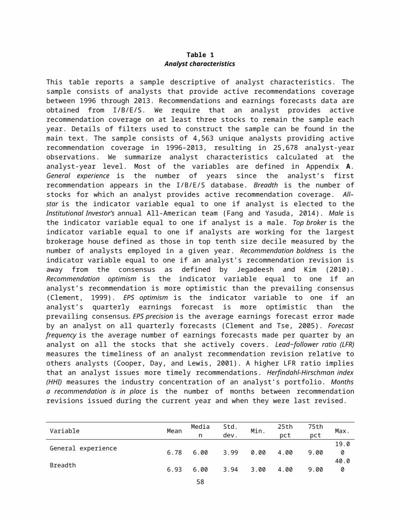
Table 1 summarizes characteristics of analysts that are in the final sample.

All variables are defined in Appendix A. We provide explanation for the

construction of selected variables in the Online Appendix, Section A. The

mean general experience for analysts in our sample is 6.78 years, while the

median is 6 years. The variable Breadth measures the number of stocks that

an analyst actively provides recommendations. On average, the number of

stocks in an analyst recommendation portfolio is 6.93. The descriptive

statistics of analyst characteristics reported in Table 1 are in line with the

literature.

The average Months recommendation is in place is 11.92 months, with a

median of 11.19 months. This key variable reflects the time that a

recommendation by an analyst remains outstanding in monthly units.

Importantly, we find the standard deviation and the percentile distribution of

this key variable shows a significant variation.

2.3 Methodology for identifying analysts’ recommendation speed-style

We classify analysts into different recommendation speed-style groups on a yearly

basis from 1996 to 2013. The method is an out-of-sample classification. For

instance, when classifying the speed of analysts in the year 2000, we use I/B/E/S

recommendations history only up until December 1999. As for the year 2001, we

extend the history file to include an additional year of recommendation-change

12

records.9 The methodology for classifying analysts into different speed-style groups

consists of the following three steps, which we discuss next.

Step 1: Estimating the time between revisions for each analyst-stock pair

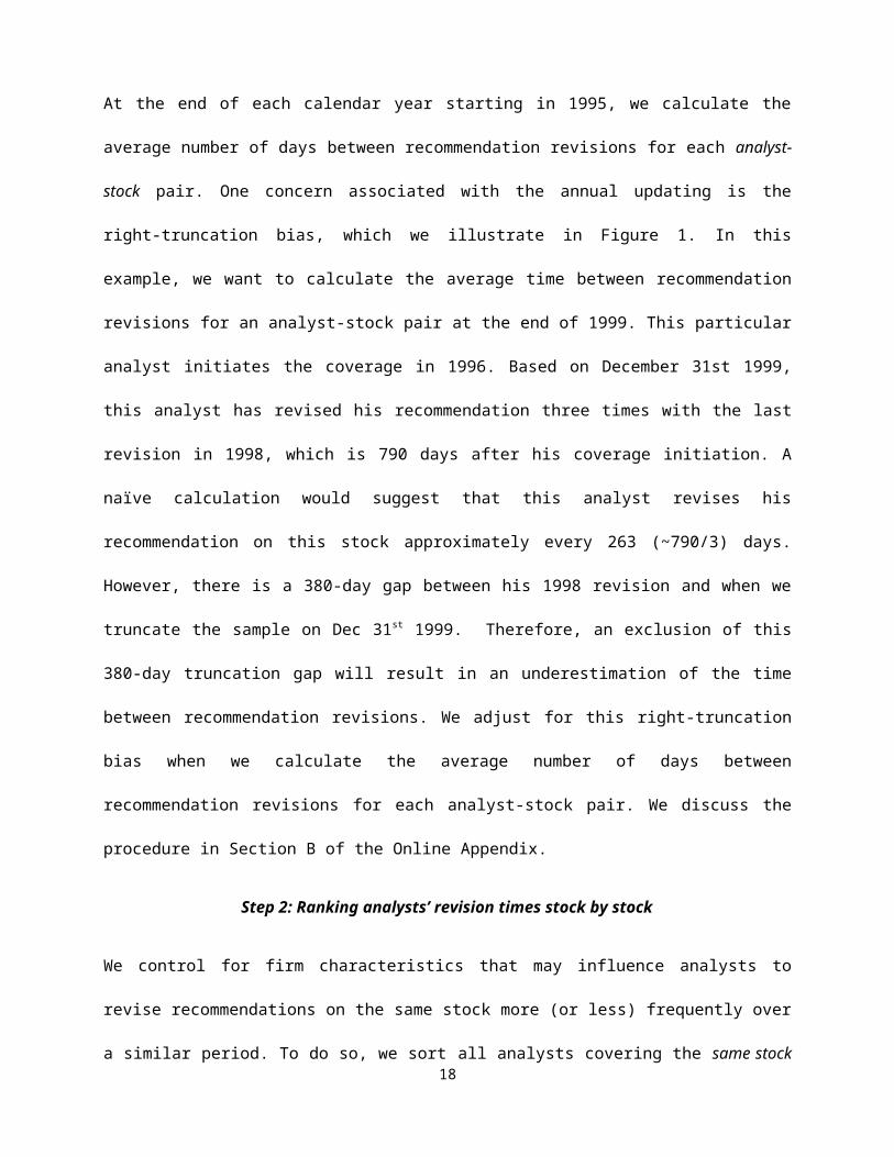
At the end of each calendar year starting in 1995, we calculate the average number

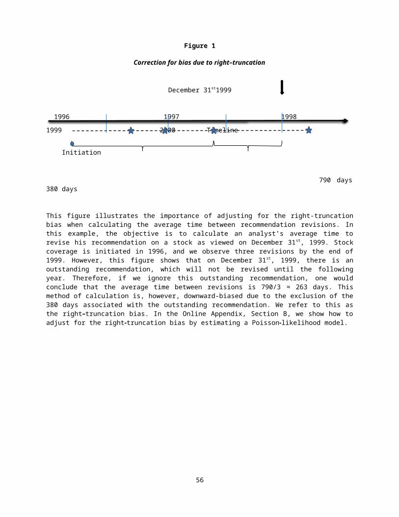
of days between recommendation revisions for each analyst-stock pair. One concern

associated with the annual updating is the right-truncation bias, which we illustrate

in Figure 1. In this example, we want to calculate the average time between

recommendation revisions for an analyst-stock pair at the end of 1999. This

particular analyst initiates the coverage in 1996. Based on December 31st 1999, this

analyst has revised his recommendation three times with the last revision in 1998,

which is 790 days after his coverage initiation. A naïve calculation would suggest

that this analyst revises his recommendation on this stock approximately every 263

(~790/3) days. However, there is a 380-day gap between his 1998 revision and

when we truncate the sample on Dec 31st 1999. Therefore, an exclusion of this 380-

day truncation gap will result in an underestimation of the time between

recommendation revisions. We adjust for this right-truncation bias when we

calculate the average number of days between recommendation revisions for each

analyst-stock pair. We discuss the procedure in Section B of the Online Appendix.

Step 2: Ranking analysts’ revision times stock by stock

We control for firm characteristics that may influence analysts to revise

recommendations on the same stock more (or less) frequently over a similar period.

To do so, we sort all analysts covering the same stock into quartiles based on their

average revisions time, i.e. from fastest (top 25th percentile) to slowest (bottom 25th

9 Our main conclusions are unaffected when using a 7-year, 5-year, or 3-year rolling window of recommendation history, instead of all past history, to classify our analysts. Section D in the Online Appendix reports robustness-check results using different rolling windows of recommendation history.

13

percentile). The sorting is done annually using the biased-adjusted time between

revisions that we calculated in Step 1.

More formally, consider the ranking of analysts’ revision speed on stock j

in year 2000. Here, we use analysts’ biased-adjusted time between

recommendation revisions that were calculated in December 1999. Letτ a , j

denote the bias-corrected average revision time of analyst a on stock j, and

assuming that there are Aj analysts covering this stock j. We sort τ a , jacross Aj

analysts into four equal groups from smallest (fastest) to largest (slowest). We

repeat this procedure for all the stocks j annually from 1996 to 2013. As we

move forward each year, an additional year of recommendation-change

records is added to the ranking method. As a result, we have out-of-sample

revision-speed rankings (from fastest to slowest quartiles) of all analyst-stock

pairs in the sample.

Step 3: Identifying the speed-style of each analyst

Using the revision-speed ranking results from Step 2, we statistically test, for each

analyst, whether he exhibits a distinct recommendation-speed pattern (i.e., fast or

slow) across all the stocks that he covers. The logic of our test is as follows: If an

analyst does not exhibit a distinct recommendation-revision speed, he should be

equally represented in all four speed quartiles. In other words, the likelihood that his

revision speed on any particular stock falls in the first (or the fourth) speed quartile

should be one-fourth. This is the null hypothesis that we test.

For instance, consider an analyst covers 8 stocks and does not have an

extreme speed-style preference, we expect probabilistically that 1/48 = 2 of

his stock-revision speeds are equally observed in one of the four quartiles

from the first (fastest) to the fourth (slowest). However, if we find 7 out of 8 14

stocks in his portfolio are ranked in the fastest revisions quartile, it is likely

that this analyst has a revision speed-style that is faster than the average

analyst. But according to this example, is 7 out of 8 a sufficient cut-off to

confidently classify that this analyst is “fast”? Importantly, analysts do not

usually cover the same number of stocks. What if this analyst covers 12

stocks instead of 8? What should the cut-off for the minimum number of

stocks that are in the fastest quartile be before we can decidedly classify him

as a “fast” analyst? We address this issue by applying the standard Binomial

test. This method helps us define the cut-offs that we can use to conclusively

classify an analyst as being distinctly “fast” or “slow” using the same

statistical criteria (0.05 p-value) regardless of the number of stocks that he

covers. Specifically, we test each of the following null hypotheses:

H0 (fast): The probability that stocks in an analyst’s portfolio are ranked in the

fastest revisions quartile is not greater than 25%.

H0 (slow): The probability that stocks in an analyst’s portfolio are ranked in the

slowest revisions quartile is not greater than 25%.

A rejection of the above hypothesis H0 (fast) at the 5 percent significant

level allows us to confidently classify an analyst as faster at revising

recommendations relative to peers.10 Similarly, a rejection of H0 (slow) at the

5 percent significant level would lead us to conclude that the analyst is slower

at revising recommendations relative to peers. Finally, we assign analysts into

three groups: (1) Slow-turnover analyst, (2) Average-turnover analyst, and (3)

Fast-turnover analyst. Analysts for whom we can reject neither of the two null

hypotheses are classified as average-turnover analysts. Figure 2 illustrates

10 Consider our prior example, where 7 out of 8 stocks in an analyst’s portfolio are in the fastest revisions quartile. According to a Binomial distribution, the probability that 7 or more stocks (out of 8) are in the fastest revision quartile, given that the null probability is 25% is less than 0.001.

15

examples of slow- versus fast-turnover analysts’ recommendation patterns on

Bank of New York Mellon Corporation (top panel), and Sunoco (bottom panel).

Here, we pick two analysts with different recommendation turnover groups

who revise their recommendations on the same stock over a similar period.

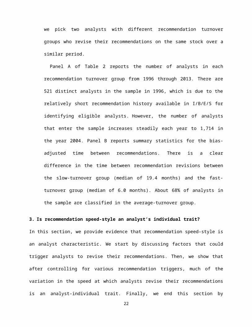
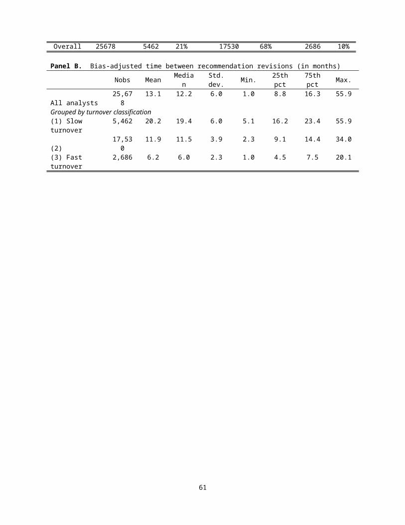
Panel A of Table 2 reports the number of analysts in each recommendation

turnover group from 1996 through 2013. There are 521 distinct analysts in

the sample in 1996, which is due to the relatively short recommendation

history available in I/B/E/S for identifying eligible analysts. However, the

number of analysts that enter the sample increases steadily each year to

1,714 in the year 2004. Panel B reports summary statistics for the bias-

adjusted time between recommendations. There is a clear difference in the

time between recommendation revisions between the slow-turnover group

(median of 19.4 months) and the fast-turnover group (median of 6.0 months).

About 68% of analysts in the sample are classified in the average-turnover

group.

3. Is recommendation speed-style an analyst’s individual trait?

In this section, we provide evidence that recommendation speed-style is an analyst

characteristic. We start by discussing factors that could trigger analysts to revise

their recommendations. Then, we show that after controlling for various

recommendation triggers, much of the variation in the speed at which analysts

revise their recommendations is an analyst-individual trait. Finally, we end this

section by examining analyst characteristics that are associated with slower and

faster recommendation-speed styles.

3.1. Triggers of recommendation revisions

16

Intuitively, we expect an analyst to upgrade (or downgrade) a stock when the ratio

of his own stock valuation to its current price (V/P) exceeds (or falls below) a certain

threshold. In this framework, several factors can speed up or delay analysts from

issuing a new recommendation. We group them into the following four channels.

These channels need not be mutually exclusive.

The first channel is the arrival of new information, which affects analysts’

assessment of the stock value (V), and thereby, can trigger recommendation

revisions. The information that analysts uncover may be public, such as

corporate disclosures. Analysts may also acquire information privately

through their interactions with firm managers or from their own research. In

the latter case, the new information that analysts uncover is not publicly

observable and hence is unknown to econometricians. We expect that the

speed at which analysts revise their recommendations is increasing with the

intensity of information arrival.

The second channel that affects the ratio of an analyst’s valuation-to-price

ratio is through the publicly traded share price (P). An increase (or fall) in the

share price lowers (raises) analysts’ own valuation-to-price ratio (V/P), which

may trigger an upgrade (or a downgrade) stock recommendation. Changes in

stock price can occur gradually or suddenly (i.e., price jumps). Such price

changes may be due to the arrival of news, and thus in this case, the price

channel is not mutually exclusive from the arrival of new information (Conrad

et al. 2006). However, sudden price changes can occur without the arrival of

news. This out-of-the-blue price adjustment can be transitory, e.g., a short-

term liquidity-related shock, or permanent, e.g., a delayed market response to

an existing information. A recommendation revision also needs not depend

17

only on the price of a security under which an analyst is evaluating. Analysts

may benchmark their stock recommendations against share prices of other

firms in the industry (i.e., the industry benchmark) or the aggregate stock

market; see Kadan et al. (2012). Relatedly, fluctuations in the share price can

affect analysts’ recommendations. When the stock price is highly volatile,

analysts’ estimates of their valuation-to-price ratio (V/P) are less precise and

could potentially delay their recommendations.

Third, the speed at which analysts revise their recommendation may

depend on the type of recommendation that analysts are evaluating. For

instance, a recommendation change by multiple notches may take longer

time to execute (i.e., from “sell” to “buy”) than a one-notch upgrade (i.e.,

from “hold” to “buy”) because a multiple-notch change would reflect a more

drastic update in the analysts’ valuation-to-price ratio. Additionally, the

current recommendation level that an analyst places on the firm can affect

the speed that he will revise it. An analyst may be more reluctant to put a firm

on a “strong sell” for an extensive period in fear of being shunned by the

firm’s management. On the other hand, an analyst may be more comfortable

with leaving his stock recommendation on “hold” for an extended period until

he uncovers fresh-new information to warrant a “buy” or “sell”

recommendation.

Finally, the fourth channel that can explain variations in the speed of

analysts’ recommendations is the analyst-person characteristic. One can

expect certain analysts to make their decisions more quickly, while others are

slower and more methodic in their valuation approaches; see Kahneman

(2011) for a summary of literature on the speed of human decision-making.

Further, variations in the speed at which analysts update their 18

recommendations may be a strategic choice. As shown in Bernhardt, Wan and

Xiao (2016), sell-side analysts strategically introduce frictions in their

recommendation decisions in order to avoid frequent revisions because

investors would otherwise question their ability.

3.2. Predicting the time to the next recommendation change

We next provide evidence that much of the variations in the speed at which analysts

revise their recommendations is an analyst-level characteristic. To demonstrate this,

we show that the recommendation speed-style that we identified using analysts’

past recommendation patterns can predict the speed at which they will revise future

recommendations after controlling for various recommendation triggers.

We estimate the Cox Proportional Hazard (Cox PH) model for the hazard

rate at which an analyst will revise his future recommendations in any given

week. The Cox PH model is commonly used in survival analysis and we prefer

it over the logistic model because it can handle censored outcome variables

(e.g., right-truncation bias as shown in Figure 1).

Let λ (t ) denote the hazard ratethat an outstanding recommendation on

stock j by an analyst a will be revised in week t, we assume that λ (t ) follows a

log-linear model:

λ ( t )=λ0 , j (t ) exp(❑Slow Slowa+❑Fast Fast a+Σi❑❑i X i , j ( t )+ηa ) . (1)

We estimate the above model at the recommendation-week level, and separately for

upgrades and downgrades. For each recommendation, we create a weekly panel

where each observation corresponds to a distinct week t, starting from when this

recommendation became outstanding until when it is revised. The weekly (rather

than daily) frequency choice is motivated by computational practicality and because

a recommendation change that occurs within one week is extremely rare, i.e., 0.06%

19

of all revisions. There are about 8.5 million weekly panel observations created from

158,210 recommendation revisions over the 1996−2013 period, where

approximately 3.5 million of them are upgrades. We estimate the model using

maximum likelihood.11

Our independent variables of interests are the two dummy variables Slow

and Fast, indicating the recommendation speed-style of each analyst that was

identified from the previous year. Slow (Fast) is equal to 1 if the analyst was

classified as the slow-turnover (fast-turnover) type in the previous year, and 0

otherwise. Year-fixed effects and previous recommendation-level fixed effects

are included in the model.

We include a series of firm-level, industry-level, and recommendation-

level controls in the Cox PH model. They are represented by Σi❑❑iX i , j(t ) in

equation (1). The baseline hazard rate function in equation (1) is assumed to

be firm specific and denoted by λ0 , j ( t ) for firm j. We allow for unobserved

heterogeneity across analysts in the Cox PH model by including analyst-

random effects. This is represented by the term ηa in equation (1). This

modeling approach is known as the frailty model, which helps control for

unobserved analyst characteristics that may affect recommendation speed

such as their private information about the firms that they cover.

A. Baseline estimation results

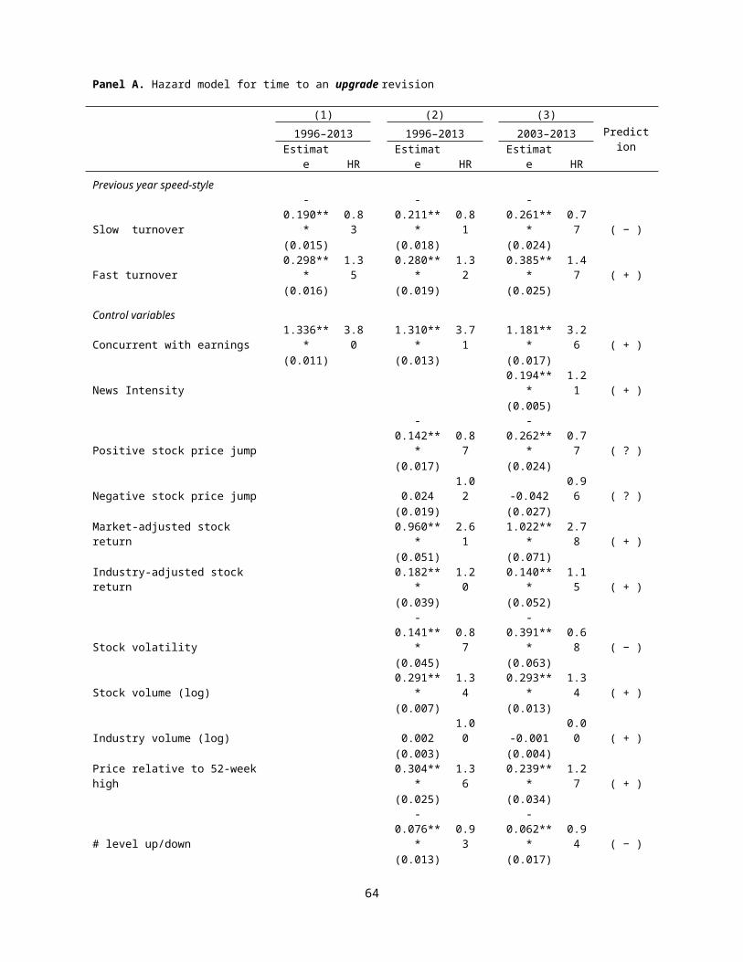
Table 3 reports the results. Panels A and B report estimates for the hazard-

rate model that the current recommendation will be upgraded and

downgraded, respectively. A positive value on the coefficient estimate

indicates that an increase in the corresponding independent variable will

11 It can take up to 24 hours to estimate each Cox PH model specification on the SAS WRDS-Cloud server with this weekly panel data over the 1996–2013 period.

20

increase the rate at which a recommendation will be revised, while a negative

coefficient estimate would indicate the otherwise.

Column (1) in Panel A and Column (4) in Panel B report the baseline model

estimates for upgrades and downgrades, respectively. Here, we include an

indicator variable Concurrent with earnings, which controls for the well-known

fact that analysts often revise their recommendations around earnings

announcements, and fixed effects that control for the previous

recommendation level.

We find that the coefficient estimate on Slow is negative, while the

coefficient estimate on Fast is positive. This finding indicates that an analyst

with a history of slow (fast) recommendation-revising pattern is likely to

revise his next recommendation more slowly (quickly) than an average-

turnover analyst, which is the reference group. We can interpret the economic

magnitude of each coefficient estimate by looking at its corresponding hazard

ratio, which is the exponent of each estimate. The hazard ratios are reported

under the column titled “HR” next to their estimates. Each hazard ratio

represents the relative increase (or decrease) in the likelihood that a

recommendation will be revised for a one-unit change in the independent

variable.

Column (1) shows the hazard ratio for Fast is 1.35, and for Slow is 0.83.

This implies that on any given week, a fast-turnover analyst is 1.35 times

more likely to upgrade a stock, on any given week, relative to an average-

turnover analyst, while for a slower-turnover analyst, the likelihood is 0.83

times lower. We can also compare the speed of recommendation changes

between slow- vs. fast-turnover analysts using their hazard ratios, i.e.,

1.35/0.83 ≈ 1.62. This suggests that on any given week, a fast-turnover

21

analyst is 1.62 times more likely to upgrade his recommendation relative to

that of a slow-turnover analyst. We find a similar economic magnitude for

downgrades. Column (4) suggests that a fast-turnover analyst is 1.41/0.82 ≈

1.72 times more likely than a slow-turnover analyst to downgrade a stock on

any given week.

The statistical importance of including the two Slow and Fast indicator

variables in the Cox PH model is large. We illustrate this by reporting the log-

likelihood ratio (LLR) comparing the likelihood of the unrestricted model that

includes the two speed-style indicators versus the likelihood of the null model

that does not. The LLR for each model specification is reported near the

bottom of Panels A and B. Columns (1) and (4) show the LLR are 688 and 916,

respectively. These values are extremely large as the critical cut-off for

rejecting the null model at the 0.001 p-value is 13.82.12

As expected, we find the estimate on Concurrent with earnings to be

positive and highly significant. We find that the probability that an analyst will

revise a recommendation is almost four times higher when there is a

concurrent earnings announcement in the same week. We include previous-

recommendation fixed effects in Table 3 using indicator variables Last recom.

The reference level for the previous-recommendation fixed effects is “hold.”

Panel A shows the coefficients on Last recom for upgrades are mostly

positive. This suggests that upgrades out of a “hold” recommendation are

stickier than upgrades out of a “strong sell” or a “sell.” In Panel B, we find

that downgrades out of a “strong buy” recommendation takes a longer time

than downgrades out of other recommendation levels.

B. Speed-style under various controls for recommendation triggers

12 The log-likelihood ratio (LLR) converges to a Chi-squared distribution with two degree of freedoms.

22

We next show that our main regression results hold after including various sets of

control variables for recommendation triggers. For brevity, we leave discussions on

how coefficient estimations on these control variables are related to analysts’

recommendation speed-style in relation to the framework that we outlined in Section

3.1 to the Online Appendix.

Columns (2) and (5) of Table 3 report the estimation results with a more

extensive set of control variables. Where applicable, all control variables are

lagged by one week, as they are potential triggers of future recommendation

revisions. We include a large set of controls for changes in the publicly traded

share prices (P). This includes an upward or a downward stock price

momentum relative to the aggregate market, i.e., Market-adjusted stock

return, or to an industry benchmark, i.e. Industry-adjusted stock return. Large

changes in share price can also occur abruptly, and they are often referred to

as jumps. We therefore include two indicator variables Positive stock price

jump and Negative stock price jump.13 We also include Stock Volatility as a

control because high volatility may lower analysts’ ability to precisely

estimate their stock valuation-to-price ratio (V/P). Finally, we include the stock

price ratio relative to its 52-week high because previous research has shown

that the 52-week high price serves as a reference point for the decisions of

traders (e.g., George and Huang, 2004). This control is represented by Price

relative to 52-week high.

In Columns (3) and (6) of Table 3, we introduce an additional variable

News intensity, which is the number of firm-specific news observed in the

13 We apply the method of Loh and Stulz (2011) to detect daily stock returns that are outliers, in a sense that they cannot be explained by the firm’s current volatility level. For each day t, we flag the security as experiencing a positive (or negative) jump if its 1-day buy-and-hold adjusted return exceeds 1.96 × σ ε (or falls below −1.96 × σ ε), where σ ε is the idiosyncratic volatility calculated using the Carhart 4-factor model over the [−60, −5] days relative to day t. We use 1.96 as the cut-off value in detecting return outliers, which corresponds to the 5 percent detection rate for a standard normal distribution.

23

previous week. It proxies for the arrival of new information that affects an

analyst’s stock valuation (V). We obtain data on news releases from Capital

IQ, a comprehensive database of company-specific news collected from over

20,000 public news sources. They include firm- and non-firm initiated news

found in newswire services. News coverage in the Capital IQ database was

relatively thin until the end of 2002. As a result, the sample that we use to

estimate the Cox PH model in Columns (3) and (6) is from 2003 to 2013.14

The time it takes an analyst to revise his recommendation can depend on

the magnitude of the recommendation change that he is evaluating. We

control for this effect in Table 3 using # level up/down, which is defined as the

absolute value of the difference between the new and previous

recommendation levels.

Overall, we find that the coefficient estimates on Slow and Fast remain

strongly significant and are in the expected direction after more controls for

recommendation triggers are added to the model. Importantly, these

estimates are similar in magnitude relative to their baseline estimates in

Columns (1) and (4). For instance, the proportion of hazard ratios for Slow and

Fast in Column (6) is 1.47/0.77 ≈ 1.9. This implies that on any given week, a

fast-turnover analyst is almost twice more likely to revise his recommendation

relative to a slow-turnover analyst. These findings indicate that analysts’ past

revision-speed patterns is a robust predictor of the rate at which they will

revise future recommendation.

3.3. Recommendation speed-style and analyst characteristics

14 See Section 5.1 for a detailed description of the Capital IQ database

24

We next examine which analyst characteristics are associated with

different recommendation speed-styles. We estimate three logit models. In

the first model, the dependent variable is an indicator function that is equal to

1 if the analyst in year t belongs to the Slow-turnover group, and 0 otherwise.

Similarly, in the second and third specifications, the dependent variable is an

indicator function that is equal to 1 if the analyst on year t belongs to the

Average-turnover and Fast-turnover group, respectively, and zero otherwise.15

Table 4 reports the results. All independent variables are analyst-level

characteristics and are defined in Appendix A. We first examine the set of

variables that are related to analysts’ career outcomes. Looking at Column

(1), we find that General Experience (the number of years since an analyst’s

first recommendation), All-star (a dummy equal to one if the analyst is

currently elected to the Institutional Investor’s All-American annual ranking),

and Top Broker (a dummy equal to if the analyst’s brokerage ranks in the top

decile by size in a given year) are positively and significantly associated with

the probability that an analyst is identified with the slow-turnover group. This

finding indicates that slow-turnover analysts tend to have better career

outcomes in the sense that they have a longer career, more likely to attain

the All-star status, and work for a top brokerage firm. Among these three

career-outcome variables, General Experience has the strongest association

with slow-turnover analysts with a t-statistic of 27. Looking at the results in

Columns (2) and (3) for the average- and fast-turnover group, we find the

coefficients on the three variables General Experience, All-star, and Top

Broker become negative. In particular, the magnitude of the coefficients and

15 We opt for this approach rather than an ordered-logit (or an ordered-probit) model because the log-likelihood-ratio test rejects the parallel regression assumption (see Long and Freese, 2014).

25

their statistical significance are the largest and strongest for the fast-turnover

group. Put together, those results show that slower decision-speed style is

associated with positive outcomes.

We next turn to the characteristics of stock recommendations that analysts

with different recommendation-speed styles make. Columns (1) and (3) of

Table 4 show the Leader-follower ratio (LFR), which measures the average

timeliness of an analyst’s recommendation change, to be positively

associated with slow-turnover analysts, but negatively with fast-turnover

analysts.16 This implies that recommendation changes of slower-revising

analysts tend to “lead the pack,” in the sense that they often front-run

recommendation changes of faster-revising analysts. Relatedly, we find that

recommendations of fast-turnover analysts tend to be less bold, i.e., they

herd more towards the consensus. This is seen in Column (3) which shows

that Recommendation boldness is negative and significant at the 5 percent

level. Overall, these findings lead to two important insights on the type of

recommendations that less frequent updaters issue; they are timelier and less

likely to herd.

We find the number of forecasts per quarter, Forecast frequency, to be

negatively associated with the probability of being classified as a fast-

turnover analyst. Thus, even though fast-turnover analysts make more

frequent recommendation changes, they tend to revise their forecasts less

frequently. This finding suggests that the decision-making of slow- and fast-

turnover analysts are inherently different. An interpretation that one can

16 We measure the timeliness of recommendation change in the spirit of Cooper, Day, and Lewis (2001) who developed the LFR to quantify the timeliness of an analyst’s forecasts. We apply their method to analysts’ recommendation revisions. A larger value of LFR value indicates the analyst, on average, issues more timely recommendation changes. See Appendix A in the Online Appendix for details.

26

make from these results is that slower-revising analysts are more reluctant to

revise their recommendations despite being more active at updating their

stock valuation-to-price ratio (V/P), on which they base their decisions. This is,

perhaps, due to the difference in thresholds that slow- vs. fast-turnover

analysts require their stock valuation-to-price ratio to exceed (or fall below)

before a new recommendation is warranted.

Finally, controlling for all other characteristics, we find Breadth —the

number of stocks covered–to be negatively associated with slow-turnover

analysts but positively correlated with fast-turnover analyst. However, in the

univariate analysis (untabulated), we find that slow-turnover analysts cover

more stocks than fast-turnover analysts do, although the difference is

economically small.

4. Investment value implications

4.1. Stock price reaction to recommendation revision

Our objective is to quantify the difference in immediate market reactions

to recommendation changes made by slow- versus fast-turnover analysts

after controlling for various factors. We estimate the following regression

model:

BHAR [−1 ;+1 ]s ,i ,t=Slowanalyst i+βAnalyst Control si , t +γRevisionControl ss , t

+δStockControl ss ,t+εs , i ,t ,

(2

)

where BHAR [−1 ;+1 ]s ,i ,t is the buy-and-hold abnormal return (BHAR) centered on the

recommendation revision made by analyst i on stock s at time t.17 The BHAR from

days t−1 to day t+1relative to the recommendation date t is calculated as follows:

17 We obtain similar conclusions if we measure the immediate price impact using the event windows [0, +1] or [0, 0] relative to the recommendation change date.

27

BHAR[−1 ,+1]=∏τ=t−1t+1 (1+R s ,τ )−∏τ=t−1

t+1 (1+RDGTW , τ) ,

whereR s ,τ is the raw return on stock s on day τ , and RDGTW , τ is the return of a

benchmark portfolio with the same size, book-to-market (B/M), and momentum

characteristics as the stock defined following Daniel, Grinblatt, Titman, and Wermers

(1997), DGTW hereafter.

Table 5 reports the results. For this analysis, we include only

recommendation changes that are made by slow- and fast-turnover analysts.

Our variable of interest here is Slow Analyst i, which is an indicator variable

equal to 1 if analyst i is a slow-turnover type, and 0 if he is otherwise a fast-

turnover type. Therefore, Slow Analyst i measures the difference in market

reaction to recommendation changes of slow-turnover analysts relative to

those of fast-turnover analysts. We include various characteristics of the

stocks on which the recommendations are issued, as well as analyst-level

characteristics (All–star, Male, and Breadth). We also include firm brokerage,

industry and year-fixed effects in the regression, and cluster standard errors

at the firm level.

Column 1 of Table 5 presents results for upgrade recommendations. We

find that, on average, an upgrade made by a slow-turnover analyst generates

a 45 basis points higher immediate market reaction than that of a fast-

turnover analyst. Column 2 presents results for downgrade recommendations.

Similarly, we find the market reacts significantly more to a recommendation

downgrade made by a slow-recommendation revising analyst; the difference

in magnitude is about 76 basis points.

Interestingly, we find that General Experience positively affects market

reaction to downgrades and that the coefficient on upgrades is not significant. 28

Therefore, all else equal, we find that the market does not react more strongly

to recommendation changes of more experienced analysts. Among various

analyst characteristics, we find that an analyst’s earnings forecast precision

predicts the immediate price impact of his recommendation changes. This is

seen from the statistically significant estimate on High EPS precision for both

upgrades and downgrades. Consistent with prior literature (e.g., Jackson,

2005; Loh and Mian, 2006), we find that analysts who previously issued more

precise earnings forecasts have greater ability to move prices. Nevertheless,

High EPS precision does not erode the strong predictability of the

recommendation speed-style.

Additionally, we find that our main conclusion holds after controlling for

characteristics that are specific to each recommendation revision. We include

dummies for recommendation revisions that occur one week before (Pre-

earnings), one week after (Earnings-related), and around the day of an

earnings announcement (Concurrent with earnings) because the timing of the

recommendation revision relative to earnings news conveys information

(Ivkovic and Jegadeesh, 2004). We include a dummy variable for revisions

that herd toward the consensus (Away from consensus) ad defined in

Jegadeesh and Kim (2010). We also control for the magnitude of the

recommendation change (# level up/down), and the recommendation level

before it is revised (Initial level). Overall, we find the predictive ability of

recommendation speed-style is economically large and significant, and more

importantly, it dominates other ex-ante analyst characteristics that have been

linked to analysts’ ability to move prices.18

18 Appendix Table A1 further verifies our results in a univariate setting by directly comparing stock price reactions to recommendations of different analysts’ speed-style groups against their experience, as well as against their All-star status.

29

4.2. Real-calendar-time portfolio strategy

We examine real-time investment value of recommendation revisions made by fast-

vs. slow-turnover analysts. We build a trading strategy that follows recommendations

issued by different analyst turnover groups. Specifically, in the spirit of Barber,

Lehavy and Trueman (2007), we design a trading strategy that invests $1 on

upgraded stocks and sells $1 on downgraded stocks.

We assume that the stock is transacted at the closing-day price after the

recommendation change. This ensures that the strategy is implementable by

ordinary investors without private access to analysts’ recommendations, i.e.,

before recommendation changes are made public. We carefully adjust for

after-trading-hour recommendation releases using their timestamps recorded

in the I/B/E/S database. For instance, a recommendation change recorded

after the market closes on Friday is pushed to the next trading day, and the

strategy is to buy/sell the stock using the Monday’s closing-day price.  We

also assume that if the recommendation is released in the last 15 minute of

the current trading day (after 3:45pm EST), it is pushed to the next trading

day. This is because IBES recommendation timestamps are often delayed

(Bradley et al., 2014), and such consideration helps make the strategy more

implementable for ordinary investors.

We create a daily portfolio that invests one dollar in each upgraded stock

and sells one dollar in each downgraded stock. Once added to the portfolio,

the stock is held for a fixed number of trading days: 30, 60, and 120. Two

distinct long-short portfolios are formed separately for the strategy that

follows fast-turnover and slow-turnover analysts. For each portfolio, we

compute the value-weighted portfolio return following Barber, Lehavy and

30

Trueman (2007). We calculate the risk-adjusted returns using the CAPM, the

Fama-French three-factor model, and the Carhart four-factor model.

Table 6 presents our results with annualized alphas. For the 30-day holding

period, the difference in alphas is between 8.5–9.5% per year, and statistically

significant at the one percent level. This confirms that analysts in the slow-

turnover group generate a greater investment value in spite of issuing fewer

recommendations. The difference in alphas generated from the long-short

trading strategy that follows fast-turnover and the slow-turnover analysts’

recommendations remains stable for 60-trading day holding period, and

decrease to about 5% for the 120-trading day holding period. Nevertheless,

the difference in alphas is statistically significant at the one percent level.

Appendix Table A2 provides detailed results on the long (“buy”) and short

(“sell”) sides of the portfolio strategy at the daily level. We find that the

strategy based on slow-turnover analysts dominates on both long and short

sides, suggesting that the superior value of recommendations made by

slower-revising analysts is not a result of short-sell constraint. In the Online

Appendix Table IA3, we provide a comparison of our real-calendar time

portfolio alphas against prior studies. Here, we find that our strategy yields

excess returns with magnitude that are comparable with those previously

documented.19 Overall, we conclude that slow-turnover analysts are able to

generate investment returns for ordinary investors that are well beyond

analysts who make more frequent recommendation revisions.

5. Understanding the source of differing investment values

19 For instance, Barber et al. (2006) finds annualized alpha from a four-factor model in the [4.03; 10.08] range for the long side and [-11.09; -5.54] for the short side.

31

We approach this in two ways. First, we ask, what types of corporate news do fast-

versus slow-turnover analysts react to when they make recommendations? Second,

we examine the contents of analysts’ recommendation reports and distinguish

between different rationales on which they base their decision.

5.1. Reaction to news and recommendation speed-style

Analysts often update their recommendations following corporate news (Ivkovic and

Jegadeesh 2004, Li et al. 2015). In this case, recommendation revisions can add

value by facilitating price discovery of the publicly observed information signal,

consistent with the general idea that sell-side analysts play an important role of

information interpreter in the financial markets (Livnat and Zhang 2012, Rubin,

Segal, and Segal 2017).

Given that the majority of recommendations are made after corporate news

releases (Li et al. 2015), the value of a recommendation revision depends on its

incremental information beyond what market participants could learn from the

preceding disclosure. In particular, news that are not based on hard figures or those

containing forward-looking information about a company (e.g., merger and

acquisitions, corporate strategy, management forecasts) are harder to interpret by

investors who do not follow the firm professionally. Thus, recommendations that are

made following these new releases are more likely to be valuable to investors

because they significantly facilitate price discovery. In other words, these

recommendations carry greater investment value because they simplify the news

contents into an unambiguous signal — “Buy”, “Hold”, or “Sell.”

On the other hand, recommendations that are revised after less ambiguous–

verifiable corporate disclosures (e.g., earnings announcements) should be less

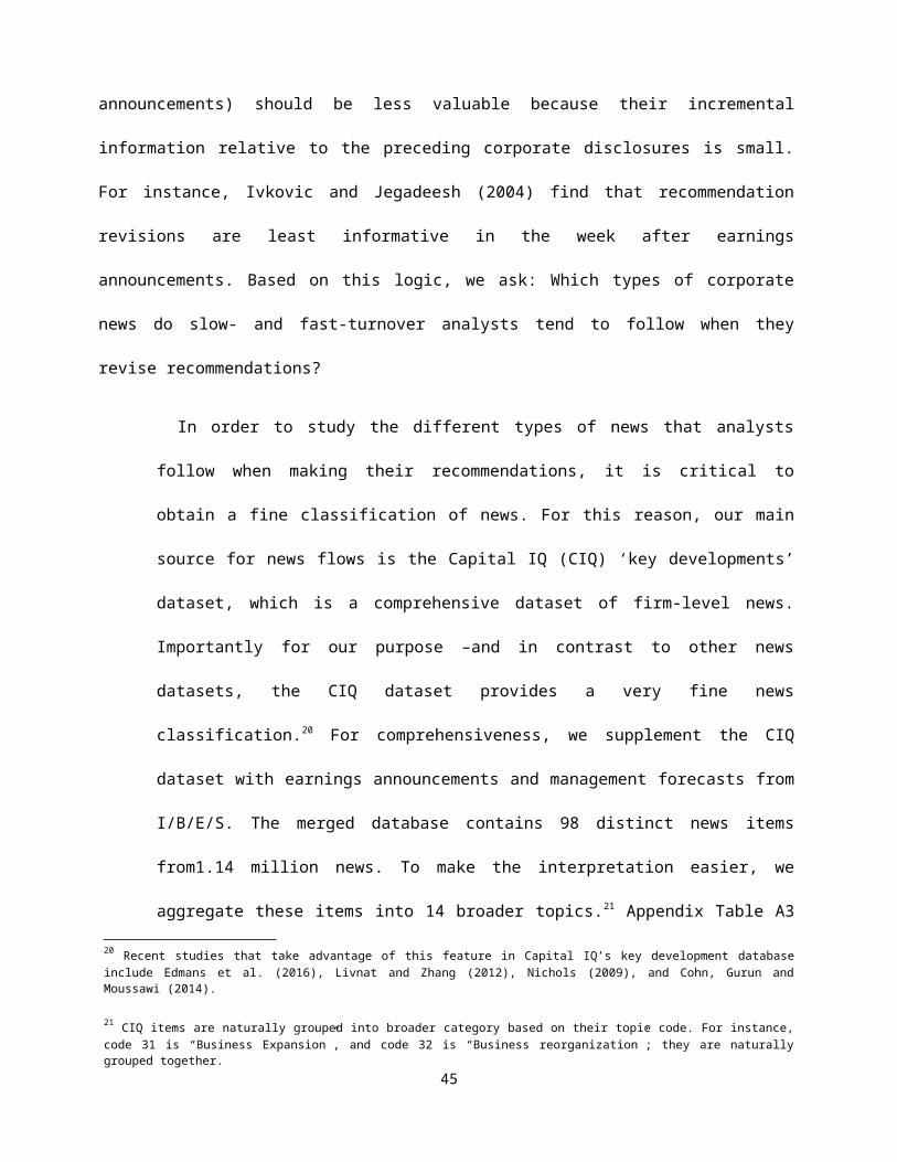
valuable because their incremental information relative to the preceding corporate 32

disclosures is small. For instance, Ivkovic and Jegadeesh (2004) find that

recommendation revisions are least informative in the week after earnings

announcements. Based on this logic, we ask: Which types of corporate news do slow-

and fast-turnover analysts tend to follow when they revise recommendations?

In order to study the different types of news that analysts follow when

making their recommendations, it is critical to obtain a fine classification of

news. For this reason, our main source for news flows is the Capital IQ (CIQ)

‘key developments’ dataset, which is a comprehensive dataset of firm-level

news. Importantly for our purpose –and in contrast to other news datasets,

the CIQ dataset provides a very fine news classification.20 For

comprehensiveness, we supplement the CIQ dataset with earnings

announcements and management forecasts from I/B/E/S. The merged

database contains 98 distinct news items from1.14 million news. To make the

interpretation easier, we aggregate these items into 14 broader topics.21

Appendix Table A3 provides the mapping of news items into the 14 news

topics. After removing topics that make up less than 1% of the dataset, there

are 9 news topics that we consider: Earnings announcements; Product market

& Operation; Management forecasts; Executive turnover; M&A; Payout policy;

Security trading; Securities issuance; and Legal issues. 22

We denote a recommendation change as being related to a specific news if

it occurs within a [0; +15] day-window after the news release. For instance,

we consider a recommendation change to be potentially triggered by a new 20 Recent studies that take advantage of this feature in Capital IQ’s key development database include Edmans et al. (2016), Livnat and Zhang (2012), Nichols (2009), and Cohn, Gurun and Moussawi (2014).

21 CIQ items are naturally grouped into broader category based on their topic code. For instance, code 31 is “Business Expansion”, and code 32 is “Business reorganization”; they are naturally grouped together.

22 Section F of the Online Appendix provides details about the database construction.

33

product announcement if it occurs within 15 days after its announcement

date. We choose the 15-day window because some news may take analysts

longer to distill their contents as well as channel checking their sources.23

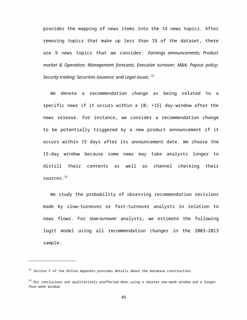
We study the probability of observing recommendation revisions made by

slow-turnover or fast-turnover analysts in relation to news flows. For slow-

turnover analysts, we estimate the following logit model using all

recommendation changes in the 2003–2013 sample:

Pr (Slow i=1 )=α+β1 .Earningsi+β2 . Product Market i+β3 .M∧A i+⋯+εi , (3)

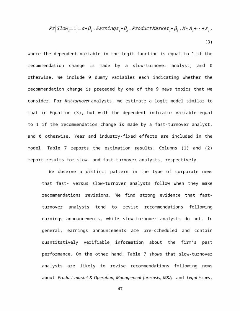
where the dependent variable in the logit function is equal to 1 if the

recommendation change is made by a slow-turnover analyst, and 0 otherwise. We

include 9 dummy variables each indicating whether the recommendation change is

preceded by one of the 9 news topics that we consider. For fast-turnover analysts,

we estimate a logit model similar to that in Equation (3), but with the dependent

indicator variable equal to 1 if the recommendation change is made by a fast-

turnover analyst, and 0 otherwise. Year and industry-fixed effects are included in the

model. Table 7 reports the estimation results. Columns (1) and (2) report results for

slow- and fast-turnover analysts, respectively.

We observe a distinct pattern in the type of corporate news that fast-

versus slow-turnover analysts follow when they make recommendations

revisions. We find strong evidence that fast-turnover analysts tend to revise

recommendations following earnings announcements, while slow-turnover

analysts do not. In general, earnings announcements are pre-scheduled and

contain quantitatively verifiable information about the firm’s past

performance. On the other hand, Table 7 shows that slow-turnover analysts 23 Our conclusions are qualitatively unaffected when using a shorter one-week window and a longer four-week window.

34

are likely to revise recommendations following news about Product market &

Operation, Management forecasts, M&A, and Legal issues, while fast-turnover

analysts do not. These four news types are often unscheduled and tend to

convey information about the firm’s future performance.

We believe that the contents of news that tend to precede

recommendations of slow-turnover analysts are not as easily interpretable by

non-stock experts. For instance, the change in product market strategy (e.g.,

new product launch, new corporate alliance) can affect the firm’s value in

different ways over the long run. Similarly, certain companies issue

management forecasts. While these forecasts help guide investors about the

firm’s future earnings or sales, they are estimates and made at the discretion

of the management team. On the contrary, the contents of earnings

announcements (i.e., EPS), which fast-turnover analysts tend to follow, can be

easily compared against analysts’ prior consensus, therefore making their

impact on stock valuation easier to quantify.

Overall, the findings in this section shed light on why analysts who revise

their stock recommendation less frequently tend to make better stock picks.

That is, recommendations of slower-revising analysts are more likely revised

following harder-to-interpret corporate disclosures. This pattern in the type of

information that slower-revising analysts take cue from allows their

recommendations to greater facilitate price discovery, and thus have better

investment value.

5.2. Rationales behind stock recommendations: Evidence from Investext

35

We provide further evidence to support the conclusion in Table 7 by analyzing

the contents in analysts’ recommendation reports downloaded from Thomson One’s

Investext.

For this analysis, we construct a matched sample of fast-turnover and slow-

turnover analysts and study their recommendation reports. The main objective for

constructing the matched sample is to mitigate potential biases that could arise due

to coverage choice of analysts and brokerage houses in Investext. Additionally, the

matched sample helps reduce the number of recommendation reports. This is

advantageous because we employ a labor-intensive approach of reading analysts’

reports, and identifying rationales and information sources behind each report. In

particular, all reports are cross-read by three researchers in order to mitigate errors

from misidentifying their contents. The final sample consists of 2,052 reports from 50

fast-turnover analysts and 50 slow-turnover analysts. These reports cover 310

distinct firms. Due to space consideration, we summarize our findings below and

leave details about the methodology and further discussions to Section G of the

Online Appendix.

The results from reading analyst recommendation reports are supportive

of our findings in Table 7, which suggest that fast- versus slow-turnover

analysts tend to follow different information signals when making their

recommendations. That is, faster-revising analysts are more likely to use

earnings based valuation to make their recommendations. On the other hand,

slower-revising analysts are more likely to base their recommendations on

news that reflect changes in the firm’s operating strategy, and product

market competition.

36

Finally, we examine whether the superior recommendation value of

slower-turnover analysts derive from their better access to management, and

thus, their ability to discover novel information. To test this, we identify the

source of information that sell-side analysts reference in their report to

support each of their recommendation rationales. While we find that slow-

turnover analysts are more likely to acquire new information through private

interactions with the firm’s senior managers, the result is not statistically

significant. We provide further discussions of this analysis in Section G of the

Online Appendix.

6. Concluding remarks

We document significant variation in how frequently sell-side security analysts

change their recommendation opinions. We develop a simple method for identifying

analysts who revise their recommendation distinctly more frequently (versus more

slowly) than their peers. We find that recommendations issued by fast-revising

analysts are heavily discounted by investors and generate significantly less risk-

adjusted investment return. Less frequent recommendation revisers are more likely

to be elected to All-star status, work at top brokerage house, and have better career

longevity.

Albeit updating their stock picks less frequently, we find that slower-

revising analysts tend to issue new recommendations that lead those of

others, i.e., “lead the pack.” Further, recommendations of slower-revising

analysts are often revised after corporate disclosures with harder-to-interpret

information, suggesting that they play a greater role in facilitating price

discovery. While we find a strong evidence that sell-side analysts are slower

to change their recommendations as their career tenure increases, decision-

37

speed is the only characteristic that predicts the investment value of analysts’

recommendations. In other words, older and more experienced analysts are

“wiser” only if they are willing to stand by to their recommendations longer.

38

References

Bae, K. H., R. M. Stulz, and H. Tan. 2008. Do Local Analysts Know More? A Cross–Country Study of the Performance of Local Analysts and Foreign Analysts. Journal of Financial Economics 88:581–606.

Barber, B., R. Lehavy, M. McNichols, and B. Trueman. 2001. Can Investors Profit from the Prophets? Security Analyst Recommendations and Stock Returns. The Journal of Finance 56:531–63.

Barber, B. M., R. Lehavy, M. McNichols, and B. Trueman. 2006. Buys, Holds, and Sells: The Distribution of Investment Banks’ Stock Ratings and the Implications for the Profitability of Analysts’ Recommendations. Journal of Accounting and Economics 41:87–117.

Barber, B., R. Lehavy, and B. Trueman. 2007. Comparing the Stock Recommendation Performance of Investment Banks and Independent Research Firms. Journal of Financial Economics 85:490–517.

Bernhardt, D., C. Wan, and Z. Xiao. 2016. The Reluctant Analyst. Journal of Accounting Research 54:987–1040.

Bradley, D., J. Clarke, S. Lee, and C. Ornthanalai. 2014. Are Analysts' Recommendations Informative: Intraday Evidence on the Impact of Timestamp Delay. The Journal of Finance 69: 645–673.

Bradshaw, M. 2011. Analysts’ Forecasts: What Do We Know After Decades of Work? Working paper, Boston College.

Clement, M. B. 1999. Analyst Forecast Accuracy: Do Ability, Resources, and Portfolio Complexity Matter? Journal of Accounting and Economics 27:285–303.

Clement, M. B., and S. Y. Tse. 2005. Financial Analyst Characteristics and Herding Behavior in Forecasting. The Journal of Finance 60:307–41.

Cohn, J. B., U. G. Gurun, and R. Moussawi. 2014. Micro-Level Value Creation Under CEO Short-Termism. Working Paper, University of Texas at Austin.

Conrad, J., B. Cornell, W.R. Landsman, and B.R. Rountree. 2006. How do analyst recommendations respond to major news? Journal of Financial and Quantitative Analysis, 41: 25-49.

Cooper, R. A., T. E. Days, and C. M. Lewis. 2001. Following the leader: a study of individual analysts' earning forecasts. Journal of Financial Economics 61: 383–416.

Daniel, K., M. Grinblatt, S. Titman, and R. Wermers. 1997. Measuring Mutual Fund Performance with Characteristics–Based Benchmarks. The Journal of Finance 52:1035–58.

Edmans, A., L. Goncalves-Pinto, Y. Wang, and M. Xu. 2016. Strategic News Releases in Equity Vesting Months. Working Paper, London Business School.

39

Fang, L. H., and A. Yasuda. 2009. The Effectiveness of Reputation as a Disciplinary Mechanism in Sell–Side Research. Review of Financial Studies 22:3735–77.

Fang, L. H., and A. Yasuda. 2013. Are Stars’ Opinions Worth More? The Relation Between Analyst Reputation and Recommendation Values. Journal of Financial Services Research :1–35.

Frankel, R., S. P., Kothari, and J. Weber. 2006. Determinants of the Informativeness of Analysts Research. Journal of Accounting and Economics 41: 29–54.

George, T.J., Hwang, C.-Y., 2004. The 52-week high and momentum investing. Journal of Finance 59, 2145-2176.

Hilary, G., and C. Hsu. 2013. Analyst Forecast Consistency. The Journal of Finance 68:271–97.

Hobbs, J., T. Kovacs, and V. Sharma. 2012. The Investment Value of the Frequency of Analyst Recommendation Changes for the Ordinary Investor. Journal of Empirical Finance 19:94–108.

Hong, H., and J.D. Kubik. 2003. Analyzing the Analysts: Career Concerns and Biased Earnings Forecasts. The Journal of Finance 58:313–51.

Ivković, Z., and N. Jegadeesh. 2004. The Timing and Value of Forecast and Recommendation Revisions. Journal of Financial Economics 73:433–63.

Jackson, A. R. 2005. Trade Generation, Reputation, and Sell–Side Analysts. The Journal of Finance 60:673–717.

Jegadeesh, N., and W. Kim. 2010. Do Analysts Herd? An Analysis of Recommendations and Market Reactions. Review of Financial Studies 23:901–37.

Kadan, O., L. Madureira, R. Wang, and T. Zach. 2009. Conflicts of Interest and Stock Recommendations: The Effects of the Global Settlement and Related Regulations. Review of Financial Studies 22:4189–4217.

Kadan, O., L. Madureira, R. Wang, and T. Zach. 2012. Analysts’ Industry Expertise. Journal of Accounting and Economics 54:95–120.

Kahneman, D. 2011. Thinking, Fast and Slow. Macmillan.

Kumar, A. 2010. Self–Selection and the Forecasting Abilities of Female Equity Analysts. Journal of Accounting Research 48:393–453.

Law, K. 2013. Career Imprinting: The Influence of Coworkers in Early Career. Working paper, Tilburg University.

Li, E. X., K. Ramesh, M. Shen, and J. S. Wu. 2015. Do Analyst Stock Recommendations Piggyback on Recent Corporate News? An Analysis of Regular‐Hour and After‐Hours Revisions. Journal of Accounting Research 53:821–61.

40

Livnat, J., Y. Zhang. 2012. Information interpretation or information discovery: which role ofanalysts do investors value more? Review of Accounting Studies 17: 612-641.

Ljungqvist, A., C. Malloy, and F. Marston. 2009. Rewriting History. The Journal of Finance 64:1935–60.

Loh, R. K., G. M. Mian. 2006. Do Accurate Earnings Forecasts Facilitate Superior Investment Recommendations? Journal of Financial Economics 80: 455–483.

Loh, R. K., and R. M. Stulz. 2011. When Are Analyst Recommendation Changes Influential? Review of Financial Studies 24:593–627.

Long, J. S., and J. Freese. 2014. Regression Models for Categorical Dependent Variables Using Stata, Third Edition. Stata Press.

Nichols, D. C. 2009. Proprietary Costs and Other Determinants of Nonfinancial Disclosures. Working Paper, Cornell University.

Prendergast, C., and L. Stole.1996. Impetuous Youngsters and Jaded Old–Timers: Acquiring a Reputation for Learning. Journal of Political Economy 104: 1105–1134.

Rubin, A., B. Segal, and D. Segal. 2017. The Interpretation of Unanticipated News Arrival nd Analysts’ Skill. Journal of Financial and Quantitative Analysis, 52:1491-1518.

Sonney, F. 2009. Financial Analysts' Performance: Sector Versus Country Specialization. Review of Financial Studies 22: 2087–131.

Womack, K. 1996. Do Brokerage Analysts’ Recommendations Have Investment Value? The Journal of Finance 51:137–67.

41

Figure 1

Correction for bias due to right–truncation December 31st1999

1996 1997 1998 1999 2000 Timeline

Initiation

790 days 380 days

This figure illustrates the importance of adjusting for the right-truncation bias when calculating the average time between recommendation revisions. In this example, the objective is to calculate an analyst’s average time to revise his recommendation on a stock as viewed on December 31st, 1999. Stock coverage is initiated in 1996, and we observe three revisions by the end of 1999. However, this figure shows that on December 31st, 1999, there is an outstanding recommendation, which will not be revised until the following year. Therefore, if we ignore this outstanding recommendation, one would conclude that the average time between revisions is 790/3 ≈ 263 days. This method of calculation is, however, downward-biased due to the exclusion of the 380 days associated with the outstanding recommendation. We refer to this as the right–truncation bias. In the Online Appendix, Section B, we show how to adjust for the right-truncation bias by estimating a Poisson-likelihood model.

42

Figure 2

Slow vs. Fast recommendation turnover analysts: Examples

This figure illustrates an example of recommendation revision made on two stocks by two different types of analysts: (1) slow-turnover analyst (solid line), and (2) fast-turnover analyst (dashed line). Slow (fast) turnover analysts are those that revise their recommendations significantly less (more) often than their comparable peers do. We classify analysts in our sample at the end of the calendar year from 1996 through 2013. See text for more details. The x-axis represents the number of years elapsed since an analyst made his first recommendation on that stock.

43

Underperform

Hold

Buy

Strong Buy

0 1 2 3

The Bank of New York Mellon Corporation

Sell

Underperform

Hold

Buy

Strong Buy

0 2 4 6Number of years since the first recommendation

Slow turnover analysts Fast turnover analysts

Sunoco

Table 1Analyst characteristics

This table reports a sample descriptive of analyst characteristics. The sample consists of analysts that provide active recommendations coverage between 1996 through 2013. Recommendations and earnings forecasts data are obtained from I/B/E/S. We require that an analyst provides active recommendation coverage on at least three stocks to remain the sample each year. Details of filters used to construct the sample can be found in the main text. The sample consists of 4,563 unique analysts providing active recommendation coverage in 1996–2013, resulting in 25,678 analyst-year observations. We summarize analyst characteristics calculated at the analyst-year level. Most of the variables are defined in Appendix A. General experience is the number of years since the analyst’s first recommendation appears in the I/B/E/S database. Breadth is the number of stocks for which an analyst provides active recommendation coverage. All–star is the indicator variable equal to one if analyst is elected to the Institutional Investor’s annual All-American team (Fang and Yasuda, 2014). Male is the indicator variable equal to one if analyst is a male. Top broker is the indicator variable equal to one if analysts are working for the largest brokerage house defined as those in top tenth size decile measured by the number of analysts employed in a given year. Recommendation boldness is the indicator variable equal to one if an analyst’s recommendation revision is away from the consensus as defined by Jegadeesh and Kim (2010). Recommendation optimism is the indicator variable equal to one if an analyst’s recommendation is more optimistic than the prevailing consensus (Clement, 1999). EPS optimism is the indicator variable to one if an analyst’s quarterly earnings forecast is more optimistic than the prevailing consensus. EPS precision is the average earnings forecast error made by an analyst on all quarterly forecasts (Clement and Tse, 2005). Forecast frequency is the average number of earnings forecasts made per quarter by an analyst on all the stocks that she actively covers. Lead−follower ratio (LFR) measures the timeliness of an analyst recommendation revision relative to others analysts (Cooper, Day, and Lewis, 2001). A higher LFR ratio implies that an analyst issues more timely recommendations. Herfindahl-Hirschman index (HHI) measures the industry concentration of an analyst’s portfolio. Months a recommendation is in place is the number of months between recommendation revisions issued during the current year and when they were last revised.

Variable Mean

Median

Std. dev. Min. 25th

pct75th pct Max.

General experience 6.78 6.00 3.99 0.00 4.00 9.0019.0

0Breadth 6.93 6.00 3.94 3.00 4.00 9.00

40.00

All-Star 0.16 0.00 0.36 0.00 0.00 0.00 1.00Male 0.89 1.00 0.31 0.00 1.00 1.00 1.00Top broker 0.40 0.00 0.49 0.00 0.00 1.00 1.00Recommendation boldness 0.51 0.50 0.20 0.00 0.39 0.63 1.00Recommendation optimism 0.42 0.42 0.22 0.00 0.28 0.56 1.00EPS optimism 0.49 0.49 0.15 0.00 0.39 0.58 1.00EPS precision 0.00 0.03 0.26 -9.08 -0.10 0.14 1.00Forecast frequency 1.79 1.84 0.36 1.00 1.60 2.05 2.50Leader-follower ratio (LFR) 2.18 1.07 2.55 0.04 0.51 2.50 8.00Industry concentration (HHI) 6.45 1.88 13.07 0.22 1.00 5.06

85.00

44

Months a recommendation is in place

11.92 11.19 5.38 0.83 7.94 14.97 46.3

0

45

Table 2

Descriptive of Recommendation Turnover Classification

This table summarizes the distribution of analysts after their speed-style classification. We classify analysts by how fast they revise their recommendations relative to their peers. The classification is done at the analyst-year level. The sample consists of analysts that provide active recommendations coverage in 1996–2013. For each year from 1996 through 2013, we assign analysts into three groups: (1) Slow-turnover analyst, (2) Average-turnover analyst, and (3) Fast-turnover analyst. Slow (fast) turnover analysts are those that revise their recommendations distinctly slower (faster) than their comparable peers. Average-turnover analysts are those that cannot be distinctly classified as either a fast- or slow-turnover type. We use analysts’ past recommendation patterns up to the previous year to identify their current-year recommendation speed-style. Panel A reports the number (and percentage) of analysts in each recommendation turnover group. Panel B reports summary statistics for the time between recommendations revisions for the overall sample, as well as for each analyst turnover group. We express time between revisions in unit months corrected for the right-truncation bias. See text for more details.

Panel A. Distribution of analysts across three recommendation-turnover groups  

Year Total(1) Slow-turnover (2) Average-

turnover (3) Fast-turnover

# % # % # %1996 521   69 13% 391 75% 61 12%1997 816   138 17% 591 72% 87 11%1998 934   193 21% 651 70% 90 10%1999 1106   241 22% 765 69% 100 9%2000 1297   293 23% 868 67% 136 10%2001 1327   281 21% 909 69% 137 10%2002 1336   269 20% 942 71% 125 9%2003 1602   285 18% 1104 69% 213 13%2004 1714   282 16% 1204 70% 228 13%2005 1692   306 18% 1186 70% 200 12%2006 1704   348 20% 1175 69% 181 11%2007 1699   365 21% 1184 70% 150 9%2008 1650   411 25% 1113 67% 126 8%2009 1638   374 23% 1117 68% 147 9%2010 1654   377 23% 1091 66% 186 11%2011 1650   390 24% 1094 66% 166 10%2012 1702   423 25% 1101 65% 178 10%2013 1636 417 25% 1044 64% 175 11%

Overall 25678   5462 21%   17530 68%   2686 10%

Panel B. Bias-adjusted time between recommendation revisions (in months)  Nobs Mean Media

nStd. dev. Min. 25th

pct75th pct Max.

All analysts 25,678 13.1 12.2 6.0 1.0 8.8 16.3 55.9Grouped by turnover classification            (1) Slow 5,462 20.2 19.4 6.0 5.1 16.2 23.4 55.9

46

turnover(2) 17,530 11.9 11.5 3.9 2.3 9.1 14.4 34.0(3) Fast turnover

2,686 6.2 6.0 2.3 1.0 4.5 7.5 20.1

47

Table 3Hazard model for predicting time to the next recommendation change

This table reports results from estimating the Cox proportional hazard model for predicting time to the next recommendation change. The model is estimated for upgrade and downgrade revisions, separately. Panel A reports results for upgrade revisions, while Panel B reports results for downgrade revisions. The rate at which each outstanding recommendation on stock j by an analyst a will be revised in week t is determined by the hazard rateλ (t ). We assume the hazard rate at which each recommendation will be revised follows a log-linear model:

λ ( t )=λ0 , j ( t ) exp(❑Slow Slowa+❑Fast Fast a+Σi❑❑i X i , j(t)+ηa ) .

The model is estimated at the recommendation-week level. We report the hazard ratio next to each estimated under the column labeled “HR”. The main variable of interests are indicator variables Slow and Fast, indicating the recommendation speed-style of the analyst obtained from the previous year. For instance, Slow (Fast) is equal to 1 if the analyst was classified as the slow-turnover (fast-turnover) type in the previous year, and 0 otherwise. We let the baseline hazard be firm specific, and denoted by λ0 , j ( t ) for firm j. We include firm-level, industry-level, and recommendation-level controls in the model; they are represented by Σi

❑❑iX i , j(t ) in the log-linear hazard rate model. We allow for unobserved heterogeneity in the hazard-rate model at the analyst level by including analyst-random effects. This is represented by ηa, which is normally distributed. Year-fixed effects are included in all regressions. Concurrent with earnings is an indicator variable equal to 1 if there is an earnings announcement in the current week t, and 0 otherwise. All other independent variables are lagged by one period. News intensity is the number of firm-specific news observed in the previous week. We obtain news database from the Capital IQ’s Key developments database and the sample period begins in 2003. Therefore, regression specifications with News intensity, i.e., Columns (3) and (6), are estimated using recommendation observations from 2003 through 2013. All other regression specifications are estimated using observations from 1996 through 2013. Positive stock price jump (Negative stock price jump) is equal to 1 if there is a positive (negative) stock price change in the previous week, and 0 otherwise. We follow the method in Loh and Stulz (2011) and define jump as a visibly large stock price change that cannot be explained by the current stock volatility level. Market-adjusted stock return is the cumulative one-month buy-and-hold stock return relative to that of the CRSP value-weighted index return observed in the previous week. Industry-adjusted stock return is the cumulative one-month buy-and-hold stock return relative to that of the industry portfolio return observed in the previous week. We classify firms into different industries following the Global Industry Classification Standard (GICS). Stock volatility is the standard deviation of daily stock return calculated over each week. Stock volume and Industry volume are log of total trading volumes on the stock and on the industry observed over the week, respectively. Price rel. to 52-week high is the ratio of the stock price to its 52-week high price. # level up/down is the absolute magnitude of the recommendation scale change as defined in IBES. Previous-recommendation-level fixed effects are represented by indicator variables Last recom. The estimate and the hazard ratio for Last recom variables are relative to the reference “hold” recommendation level, i.e., 3 in the I/B/E/S code. No observations report the number of recommendation-week observations used in the estimation. No recomm changes report the number of recommendation revisions present in the estimation. Near the end of each column, we report the log-likelihood ratio comparing the unrestricted model (reported model) against to the null model that restrict Slow and Fast indicators to be 0.

48

Standard error is reported in parentheses below each estimate. ***, **, and * correspond to statistical significance at the 1, 5, and 10 percent levels, respectively.

49

Panel A. Hazard model for time to an upgrade revision         

  (1)   (2)   (3)Predictio

n  1996–2013   1996–2013   2003–2013

 Estimat

e HR  Estimat

e HR  Estimat

e HRPrevious year speed-style                  

Slow turnover

-0.190**

*0.83  

-0.211***

0.81  

-0.261**

*0.77 ( − )

  (0.015)     (0.018)     (0.024)    

Fast turnover0.298**

*1.35   0.280***

1.32  

0.385***

1.47 ( + )

  (0.016)     (0.019)     (0.025)    

Control variables                  

Concurrent with earnings1.336**

*3.80   1.310***

3.71  

1.181***

3.26 ( + )

  (0.011)     (0.013)     (0.017)    

News Intensity            0.194**

*1.21 ( + )

              (0.005)    

Positive stock price jump      -

0.142***0.87  

-0.262**

*0.77 ( ? )

        (0.017)     (0.024)    

Negative stock price jump       0.0241.02   -0.042

0.96 ( ? )

        (0.019)     (0.027)    

Market-adjusted stock return       0.960***2.61  

1.022***

2.78 ( + )

        (0.051)     (0.071)    

Industry-adjusted stock return       0.182***1.20  

0.140***

1.15 ( + )

        (0.039)     (0.052)    

Stock volatility      -

0.141***0.87  

-0.391**

*0.68 ( − )

        (0.045)     (0.063)    

Stock volume (log)       0.291***1.34  

0.293***

1.34 ( + )

        (0.007)     (0.013)    

Industry volume (log)       0.0021.00   -0.001

0.00 ( + )

        (0.003)     (0.004)    

Price relative to 52-week high       0.304***1.36  

0.239***

1.27 ( + )

        (0.025)     (0.034)    

# level up/down      -

0.076***0.93  

-0.062**

*0.94 ( − )

        (0.013)     (0.017)    

Previous recommendation level                  

Last recom. = 2 ("Buy")0.112**

*1.12   0.103***

1.11   0.037

1.04  

  (0.013)     (0.014)     (0.027)    Last recom. = 4 ("Sell") 0.362** 1.4   0.298*** 1.3   0.343** 1.4  

50

* 4 5 * 1  (0.015)     (0.015)     (0.021)    

Last recom. = 5 ("Strong sell")0.432**

*1.54   0.507***

1.66  

0.539***

1.71  

  (0.019)     (0.020)     (0.028)    

Year-fixed effects Yes Yes YesAnalyst-random effects Yes Yes YesLog-like ratio: unrestricted vs. null 688   592   502  No observations 3,514,094   2,771,067   1,669,989  No of recomm changes 71,533   62,327   36,011  

51

Panel B. Hazard model for time to a downgrade revision

  (4)   (5)   (6)Predictio

n  1996–2013   1996–2013   2003–2013

 Estimat

e HR  Estimat

e HR  Estimat

e HRPrevious year speed-style                  

Slow turnover-

0.204***0.82  

-0.204***

0.82  

-0.285***

0.75 ( − )

  (0.013)     (0.017)     (0.023)    

Fast turnover 0.347***1.41   0.350***

1.42   0.484***

1.62 ( + )

  (0.014)     (0.018)     (0.024)    

Control variables                  

Concurrent with earnings 1.343***3.83   1.291***

3.64   1.212***

3.36 ( + )

  (0.010)     (0.012)     (0.017)    

News Intensity             0.214***1.24 ( + )

              (0.005)    

Positive stock price jump       -0.0180.98   -0.032

0.97 ( ? )

        (0.016)     (0.023)    

Negative stock price jump      -

0.213***0.81  

-0.283***

0.75 ( ? )

        (0.017)     (0.025)    

Market-adjusted stock return      -

1.844***0.16  

-1.496***

0.22 ( − )

        (0.049)     (0.075)    

Industry-adjusted stock return      -

0.235***0.79  

-0.424***

0.65 ( − )

        (0.030)     (0.046)    

Stock volatility      -

0.338***0.71  

-0.373***

0.69 ( − )

        (0.036)     (0.056)    

Stock volume (log)       0.301***1.35   0.319***

1.38 ( + )

        (0.007)     (0.012)    

Industry volume (log)       -0.007**0.99   -0.007

0.99 ( + )

        (0.003)     (0.004)    

Price relative to 52-week high      -

0.504***0.60  

-0.355***

0.70 ( − )

        (0.026)     (0.039)    

# level up/down      -

0.088***0.92   -0.013

0.99 ( − )

        (0.012)     (0.018)    

Previous recommendation level                  

Last recom. = 1 ("Strong buy")-

0.059***0.94  

-0.048***

0.95   -0.016

0.99  

  (0.013)     (0.016)     (0.022)    

Last recom. = 2 ("Buy") 0.042***1.04   0.097***

1.10   0.016

1.02  

  (0.013)     (0.016)     (0.021)    

Last recom. = 4 ("Sell") 0.394***1.48   0.441***

1.56   0.449***

1.57  

52

  (0.056)     (0.066)     (0.079)    

Year-fixed effects Yes Yes YesAnalyst-random effects Yes Yes YesLog-like ratio: unrestricted vs. null 916 690 607No observations 4,982,311 3,785,808 2,154,161No of recomm changes 86,677 73,793 39,706

53

Table 4Analyst characteristics and recommendation speed-style

We report estimation results from a logistic model examining characteristics that are associated with an analyst being classified into each of the three speed-style groups (1) Slow to (2) Average to (3) Fast. The logit model is estimated at the analyst-year level. For each year from 1996 through 2013, we assign analysts into three groups: (1) Slow-turnover analyst, (2) Average-turnover analyst, and (3) Fast-turnover analyst. The dependent indicator variables in Columns (1), (2), and (3) are equal to 1 if the analyst is identified with the slow-, average-, and fast-turnover group, respectively, in that year. All analyst characteristics are calculated yearly for each analyst; see Appendix A for definitions. Year fixed effects are included in the estimation. Robust standard error clustered at the brokerage-year level is reported in parenthesis below each estimate. Each regression model contains 25,678 analyst-year observations. ∗, ∗∗, ∗∗∗ indicate significance at the 10%, 5%, and 1% level, respectively.

Logit model for the likelihood that the analyst is related with the following recommendation speed-style

  (1) Slow

(2) Average

(3) Fast

General experience 0.188*** −0.035*** −0.304***(0.007) (0.006) (0.013)

All-star 0.506*** −0.204*** −0.858***(0.056) (0.050) (0.107)

Top broker 0.265*** −0.017 −0.388***(0.052) (0.038) (0.058)

Breadth −0.031*** 0.007 0.060***(0.005) (0.005) (0.007)

Recomm optimism −0.154* 0.044 0.243**(0.093) (0.073) (0.104)

Recomm boldness 0.002 0.130 −0.417***(0.108) (0.084) (0.108)

EPS optimism 0.012 0.015 −0.068(0.123) (0.102) (0.146)

EPS precision 0.045 0.046 −0.178**(0.077) (0.056) (0.074)

Lead/follow ratio (LFR) 0.026*** 0.006 −0.064***(0.007) (0.006) (0.011)

Forecast frequency 0.102 0.086 −0.383***(0.067) (0.056) (0.086)

Male 0.023 −0.019 0.009(0.055) (0.046) (0.072)

Industry concentration (HHI) −0.001 0.000 0.000

(0.001) (0.001) (0.002)Year-fixed effects Yes Yes YesBroker-year clustering Yes Yes YesNobs. 25,678 25,678 25,678

54

Table 5Stock Price Reaction to Recommendation Changes: Regression analysis

The sample consists of recommendation changes issued by slow-turnover and fast-turnover analysts from 1996 through 2013. All control variables are defined in Appendix A. Standard errors are clustered at the firm level. ∗, ∗∗, and∗∗∗ indicate significance at the 10%, 5%, and 1% level, respectively.

  Dependent Variable: BHAR( −1,+1)  (1) Upgrade (2) DowngradeRecommendation turnover    

Slow Analyst 0.464** −0.758***  (0.218) (0.205)Stock-level characteristics    

Size −0.799*** 0.454***  (0.093) (0.065)Volatility 0.250*** −0.239***  (0.071) (0.060)Institutional investor (quartiles) −0.591*** −0.547***  (0.222) (0.145)Stock return −2.021** 0.999***  (0.999) (−2.020)Market return 6.356*** 2.062***

  (2.062) (3.080)Analyst characteristic    

General experience 0.003 0.100***  (0.025) (0.032)All-star 0.551 −0.012  (0.556) (0.258)Male 0.154 0.297  (0.223) (0.293)Breadth −0.009 0.015  (0.012) (0.014)High EPS precision 0.396** −0.269  (0.179) (0.177)High EPS optimism −0.162 0.219

  (0.207) (0.174)Recommendation-level characteristic    

# level up/down 1.124*** −1.226***  (0.195) (0.231)Initial level −0.372*** 0.168  (0.122) (0.156)Concurrent with earnings announ. 0.987*** −2.491***  (0.281) (0.308)Earnings-related revision −0.830*** 0.694**  (0.251) (0.297)Pre-earnings revision 0.584 0.773  (0.382) (0.605)Away from consensus 0.462** −1.279***

  (0.186) (0.234)Industry, Year, and Broker-fixed effects Yes YesFirm-level clustering Yes YesNobs 15,328 17,657Adjusted R-squared 13.6% 14.5%

55

Table 6

Real-calendar time Portfolio Results

This table presents annualized risk-adjusted returns of calendar-time portfolios earned by investors trading on analyst recommendations. We report annualized alphas of 30, 60, and 120-day holding period returns earned by an investor who invests $1 on a stock at the closing-day price after the recommendation upgrade and sells $1 on a stock at the closing-day price after the recommendation downgrade. The sample consists of recommendation changes issued by slow and fast-turnover analysts in our classification sample (see Table 2) from 1996 through 2013. Portfolios are formed over the 1996–2013 period and their returns are calculated daily. We report results for three holding periods: 30, 60, and 120 trading days. We report portfolio alphas from the trading strategy that follows two groups of analysts: Slow-turnover analyst, and Fast-turnover analyst. Abnormal returns are calculated using three benchmarks: CAPM, the Fama-French three-factor model, and the Carhart four-factor model. For each model, we report the constant alpha expressed in annualized percentage terms together with its t–stat. The rows labeled “Slow vs. Fast” report the difference in annualized alphas from portfolios earned by investing following recommendation changes of slow-turnover analysts minus fast-turnover analysts.

Analyst turnover type

 Holding period (trading days)

Annualized portfolio alpha (%)

   CAPM t-

stat  Fama-French

three-factort-

stat  Carhart

four-factor

t-stat

Slow   30   27.9 9.95   27.7 7.32   25.8 7.57Fast   30   18.4 7.48   18.5 7.51   17.3 7.14Slow vs. Fast 30   9.5 2.54   9.2 2.47   8.5 2.35                       

Slow   60   22.010.4

5   21.910.3

9   20.110.0

9Fast   60   9.9 7.15   13.1 7.14   11.9 6.68Slow vs. Fast 60   12.2 4.35   8.8 3.14   8.3 3.09                       Slow   120   14.7 9.47   14.7 9.50   13.2 9.19Fast   120   9.9 7.25   9.8 7.21   8.7 6.73Slow vs. Fast 120   4.8 2.35   5.0 2.42   4.6 2.36                       

56

Table 7Analyst Reaction to News

We report estimation results from a logistic model for the probability that a recommendation change is issued by a Slow-turnover analyst (Column (1)) or a Fast-turnover analyst (Column (2)). The sample consists of recommendation changes by analysts across different recommendation speed-style from 2003–2013. The dependent variable is equal to 1 when the recommendation change is from a slow-turnover analyst (or fast-turnover analyst). All independent variables are indicator functions for various news type. Each independent variable is equal to 1 if its corresponding news was issued in the [−15, 0] calendar-day window before the recommendation change, and 0 otherwise. We consider 9 different types of news leading to a recommendation change: Earnings announcement; Product market & Operation; Management forecasts; M&A; Payout policy; Securities issuance; Legal issues; Security trading; Executive turnover. Earnings announcements and earnings guidance are from the I/B/E/S actual and guidance files, respectively. All other news events are from the Capital IQ “key development” dataset. See Appendix Table A3 for a definition of news from Capital IQ. Industry and year-fixed effects are included in the estimation. Robust standard error clustered at the firm level is reported in parenthesis below each estimate. ∗, ∗∗, ∗∗∗ indicate significance at the 10%, 5%, and 1% level, respectively.

News leading recommendation Probability that the recommendation change is from:Slow-turnover analyst Fast-turnover analyst

(1) (2)Earnings announcement −0.079*** 0.045**

(0.027) (0.022)Product market & Operation 0.097*** −0.065**

(0.025) (0.033)Management forecasts 0.067** −0.124***

(0.028) (0.034)M&A 0.046* −0.084** (0.028) (0.035)Legal issues 0.122*** −0.116**

(0.044) (0.057)Executive turnover 0.057* −0.002

(0.031) (0.036)Payout policy −0.095*** 0.028

(0.031) (0.034)Securities issuance 0.025 0.201***

(0.049) (0.051)Security trading −0.016 0.072

(0.063) (0.069)Industry & Year-fixed effects Yes YesFirm-level clustering Yes YesNobs. 76,229 76,229No. of dependent var. = 1 11,650 10,499Pseudo R-squared 2.02% 4.54%

57

Appendix A: List of Variables

Variable Definition SourceAnalyst–level variablesGeneral experience The number of years since an analyst’s first recommendation

in the database to the current recommendation.I/B/E/S

Recommendation optimism

Recommendation boldness

Average annual number of an analyst’s new recommendation changes that are above, i.e. more optimistic than, the consensus. See Clement (1999), and Hong and Kubik (2003). For more details, see Online Appendix, Section A.

The average number of recommendation changes that move away from the consensus. The recommendation consensus is calculated as the mean of outstanding recommendations issued on each stock, excluding the analyst’s own recommendation. See Jegadeesh and Kim (2010). For more details, see Online Appendix, Section A.

I/B/E/S

I/B/E/S

All–star Dummy variable equal to one if an analyst is currently elected to the Institutional Investor’s All-American team annual rankings. This dummy is updated annually as the new ranking is announced.

Fang and Yasuda (2014)

Male Dummy variable equal to one if the analyst is a male and zero otherwise.

Law (2013), Kumar (2010)

Forecast frequency Number of earnings forecasts made by an analyst per stock per quarter, averaged across all stocks an analyst covers in a given year. See Clement and Tse (2005).

I/B/E/S

Top broker Dummy variable equal to one if the analyst’s brokerage house in a given year is in the top tenth size-percentile measured by the number of analysts employed in a given year. See Clement (1999).

I/B/E/S

Breadth Number of stocks an analyst provides active recommendation coverage in a given year.

I/B/E/S

EPS optimism The average number of quarterly earnings forecasts that is above the consensus, excluding the analyst’s own previous forecast level. For more details, see Appendix B.

I/B/E/S

EPS precision The difference between the absolute forecast error of analyst i forecasting firm j’s fiscal quarter Q earnings and the average absolute forecast error across all analyst forecasts of firm j’s fiscal quarter Q earnings, divided by the average absolute forecast error across all analyst forecasts of firm j’s fiscal quarter Q earnings. This figure is multiplied by (−1) and averaged across all stocks an analyst covers in a given year. a higher value of this variable indicates higher precision of an analyst’s forecasts. See Clement and Tse (2005) and Bae, Stulz and Tan (2008). For more details, see Online Appendix, Section A.

I/B/E/S

58

Appendix A: List of Variables (Continued…)

Variable Definition Source

Analyst–level variables (continued…)Leader–follower ratio (LFR)

The ratio of expected arrival times of other analysts’ recommendations during the pre- and post-recommendation periods issued by an analyst. This ratio measures the average timeliness of an analyst recommendation relative to others. A higher value of LFR indicates that the analyst is a leader in revising recommendations. See Cooper, Day, and Lewis (2001). See Online Appendix, Section A for further details.

I/B/E/S

Industry concentration (HHI)

Herfindahl–Hirschman index (HHI) measuring industry concentration of an analyst’s portfolio. A higher value of HHI indicates that the analysts’ coverage is more dispersed across industries. The first digit of SIC code is used for industry classification (see Sonney, 2007). See Online Appendix, Section A for further details.

CRSP

Stock–level variablesSize The logarithm of market capitalization CRSP

Volatility Standard deviation of residuals from the Cahart 4–factor model estimated using daily returns over [−60,−5] period relative to event date.

CRSP

Recommendation–level variables

Days a recommendation is in place

Log (#days since last recommendation)

Number of calendar days between the current recommendation revision and when it was last revised.

Log of number of calendar days since the recommendation was revised to the current date.

I/B/E/S

I/B/E/S

Initial level The level of the recommendation before the revision. I/B/E/S

# level up/down The difference between the final and the initial recommendation level

I/B/E/S

Concurrent with earnings

Dummy variable equal to one for a recommendation change that occurs on days [−1,+1] relative to earnings announcement.

I/B/E/S

Earnings–following revision

Dummy variable equal to one for a recommendation change that occurs on days [+2, +7] relative to earnings announcement.

I/B/E/S

Earnings–leading revision

Dummy variable equal to one for a recommendation change that occurs on days [−7, −2] relative to earnings announcement.

I/B/E/S

Away from consensus Dummy variable equal to one for a recommendation change that moves away from the consensus. Recommendation consensus is calculated as the mean of outstanding recommendations issued on each stock, excluding the

I/B/E/S

59

analysts’ own recommendation level.

60

Appendix Table A1

Recommendation turnover Vs. Other ex-ante measures of analyst ability

This table reports immediate stock price reactions to recommendation changes. We sorted the results with respect to recommendation turnover groups, analysts’ career tenure (i.e., general experience), and their All-star status in the annual Institutional Investor’s ranking. We measure immediate price reaction using cumulative buy-and-hold abnormal returns (BHAR) from day −1 to +1 relative to the recommendation change date. The sample consists of recommendation changes issued by analysts in our classification sample (see Table 2) from 1996 through 2013. BHAR is calculated relative the DGTW benchmark. Panels A and B report average BHAR(−1, +1) for upgrades and downgrades, respectively. Within each panel, we report two sets of double-sorted results: (1) Recommendation turnover vs. General experience, and (2) Recommendation turnover vs. All-star status. General experience is the number of years since the analyst’s first recommendation appears in the I/B/E/S database. We sort analysts annually into three equal groups based on their general experience, i.e. number of years in their career tenure: Low, Mid-career, and High. All–star is the indicator variable equal to one if an analyst is elected to the Institutional Investor’s annual All-American team (Fang and Yasuda, 2014). Recommendation turnover corresponds to our classification of analysts’ recommendation speed-style, which is based on how quickly (or slowly) they revise their recommendations relative to their peers (speed-style turnover status). Heteroscedasticity-adjusted standard error and the number of observation are reported below each estimate. The last row in each panel reports the difference and p–value of BHAR(−1, +1) between slow turnover and fast turnover. The column labeled “Older – Younger” (“All-star – Non-star”) reports the difference and p–value of BHAR(−1,+1) between older versus younger (All-star versus non-All-star) analysts. ∗, ∗∗, and ∗∗∗ indicate significance at the 10%, 5%, and 1% level, respectively.

61

Appendix Table A1. Recommendation turnover Vs. Other ex-ante measures of analyst abilityturnover (continued…)

Panel A. Upgrades: Buy-and-hold abnormal returns (BHAR) from day −1 to +1  Sorted by General experience   Sorted by All-star status

  Low Mid-career High High – Low   Non-star All-star All-star – Non-star  p–value   p–value

All analysts 2.82%*** 3.17%*** 2.91%*** 0.08%   2.90%*** 3.32%*** 0.42%***Std. error (0.001) (0.001) (0.001) 0.397   (0.000) (0.001) 0.000

Nobs. 16,788 14,625 15,826     40,412 6,827  Sorted by analysts' turnover              (1) Slow-turnover 3.64%*** 3.70%*** 3.14%*** −0.50%   3.33%*** 3.56%*** 0.23%

Std. error (0.002) (0.002) (0.002) 0.182   (0.001) (0.004) 0.2748Nobs. 1,431 1,811 3,746     2,727 1,840  

(2) Average-turnover 3.22%*** 3.17%*** 2.92%*** −0.30%***   3.06%*** 3.31%*** 0.25%**Std. error (0.001) (0.001) (0.001) 0.007   (0.000) (0.001) 0.0112

Nobs. 10,126 11,169 10,928     27,648 4,575  (3) Fast-turnover 1.84%*** 2.62%*** 2.01%*** 0.17%   1.98%*** 2.59%*** 0.60%

Std. error (0.001) (0.002) (0.002) 0.447   (0.001) (0.003) 0.116Nobs. 5,231 1,645 1,152     7,497 531  

Slow − Fast 1.80%*** 1.08%*** 1.13%***     1.34%*** 0.97%**  p–value 0.001 0.005 0.001     0.001 0.049  

Panel B. Downgrades: Buy-and-hold abnormal returns (BHAR) from day −1 to +1  Sorted by General experience   Sorted by All-star status

  Low Mid-career High High– Low   Non-star All-star All-star – Non-star  p–value   p–value

All analysts −3.28%*** −3.54%*** −3.16%*** 0.12%   −3.28%*** −3.55%*** −0.27%**  (0.001) (0.001) (0.001) 0.219   (0.000) (0.001) 0.012

  19,477 16,355 17,227     45,516 7,543  Sorted by analysts' turnover              (1) Slow-turnover −4.18%*** −3.87%*** −3.39%*** 0.79%**   −3.61%*** −3.97%*** −0.36%***

Std. error (0.003) (0.002) (0.001) 0.026   (0.001) (0.002) 0.005Nobs. 1,853 2,170 4,165     6,137 2,051  

(2) Average-turnover −3.76%*** −3.58%*** −3.18%*** 0.58%***   −3.51%*** −3.48%*** 0.04%Std. error (0.001) (0.001) (0.001) 0.00   (0.001) (0.001) 0.320

Nobs. 11,964 12,322 11,804     31,151 4,939  (3) Fast-turnover −1.97%*** −2.87% −2.20% −0.23%   −2.16%*** −2.69% −0.53%

Std. error (0.001) (0.002) (0.002) 0.341   (0.001) (0.003) 0.482Nobs. 5,660 1,863 1,258     8,228 553  

Slow − Fast −2.21%*** −1.00%*** −1.19%***     −1.44%*** −1.27%***  p–value 0.001 0.0015 0.001     0.001 0.001  

62

Appendix Table A2Real-calendar time Portfolio Strategy: Detailed Results

This table presents risk-adjusted returns of real-calendar time portfolios earned by investors trading following analyst recommendations. We report daily portfolio returns and alphas earned by buying (selling) $1 on a stock at the closing -day price after the recommendation upgrade (downgrade). We report results for three holding periods: 30, 60, and 120 trading days. Panels A and B report results for the portfolio strategy that follows recommendation changes issued by slow-turnover analysts and fast-turnover analysts, respectively, from 1996 through 2013. Analyst turnover classification are shown in Table 2. Portfolios are formed over the 1996–2013 period and their returns are calculated daily. For each holding period, we report results for a long only, short only, and a long-short portfolio strategy. For a long (short) only strategy, only recommendation upgrades (downgrades) are considered. We report t-statistic next to each alpha estimate. Abnormal returns are calculated using three benchmarks: CAPM, Fama-French three-factor model, and Carhart four-factor model.

Holding period

 Portfolio

type

  Average daily

number of firms

Number of daily return observations

Raw return (%)

  Daily portfolio alpha (%)

 CAPM t-

stat

Fama French three-factor

t-stat

Carhart four-factor

t-stat

Panel A. Slow-turnover analyst30 days Long 62 4,280 0.072 0.047 5.17 0.040 5.09 0.044 5.57

Short 79 4,280 −0.038−0.06

4−5.8

0 −0.070−6.8

4 −0.059−6.3

3Long−Shor

t 141 4,280 0.1110.11

1 9.95 0.110 9.89 0.102 9.53

60 days Long 124 4,280 0.046 0.020 2.58 0.013 2.12 0.016 2.60

Short 156 4,280 −0.041−0.06

7−7.1

3 −0.074−8.8

9 −0.064−8.6

7Long−Shor

t 279 4,280 0.0880.08

710.4

5 0.08710.3

9 0.08010.0

9

120 days Long 245 4,280 0.032 0.005 0.74 0.002 0.32 0.001 0.10

Short 304 4,280 −0.027−0.05

3−6.3

6 −0.060−8.8

6 −0.052−8.6

4Long−Shor

t 549 4,280 0.0580.05

8 9.47 0.059 9.50 0.053 9.19Panel B. Fast-turnover analyst30 days Long 71 4,279 0.058 0.031 2.98 0.022 2.48 0.027 3.07

Short 81 4,280 −0.016−0.04

2−3.8

8 −0.051−5.2

6 −0.042−4.6

2Long−Shor

t 152 4,279 0.0730.07

3 7.48 0.073 7.51 0.069 7.14

60 days   Long   142 4,279 0.025   0.012 1.27   0.003 0.38   0.007 0.95    Short   159 4,280 −0.014   −0.04 −4.1   −0.049 −5.8   −0.040 −5.1

63

1 2 0 9

   Long−Shor

t   301 4,279 0.039  0.05

2 7.15   0.052 7.14   0.047 6.68                               

120 days   Long   280 4,279 0.025  −0.00

2−0.2

8   −0.011−1.6

4   −0.008−1.2

5

    Short   312 4,280 −0.014  −0.04

1−4.5

8   −0.050−6.6

0   −0.043−6.0

7

   Long−Shor

t   593 4,279 0.039  0.03

9 7.25   0.039 7.21   0.034 6.73

64

Appendix Table A3. Capital IQ–I/B/E/S News Dictionary

This table provides the mapping between the Capital IQ’s Key Development items and I/B/E/S news to our 14 news categories. The Capital IQ dataset classifies news into various items with a label and numeric code. We supplement the Capital IQ database with I/B/E/S earnings announcements and management forecasts data. We group various news items into 14 categories: Earnings announcement; Management forecasts; Product market & Operations; Payout policy; Executive turnover; Securities issuance; M&A; Restatement and auditing; Agenda communication; Legal issues; Shareholder activism; Bankruptcy; Security trading; and Other.

News Category Sources: I/B/E/S datasets and Capital IQ’s Key development labels

Earnings announcements

I/B/E/S actual file anndats_act variableAnnouncements of Earnings (28)

Management forecasts

I/B/E/S global estimates file announce_dt variableCorporate Guidance - Lowered (26), Corporate Guidance - Raised (27), Corporate Guidance - New/Confirmed (29)

Product market & Operation

Discontinued Operations/Downsizings (21), Strategic Alliances (22), Client Announcements (23), Business Expansions (31), Business Reorganizations (32), Product-Related Announcements (41), Labor-related Announcements (44), Considering Multiple Strategic Alternatives (63), Announcements of Sales/Trading Statement (138)

Payout policy Buybacks (36), Dividend Affirmations (45), Dividend Increases (46), Dividend Decreases (47), Special Dividend Announced (94), Dividend Cancellation (213), Dividend Initiation (214), Preferred Dividend (215), Buyback Update (151), Potential Buyback (152)

Executive turnover Executive/Board Changes - Other (16), Executive Changes - CEO (101), Executive Changes - CFO (102)

Securities issuance Debt Financing Related (42), Private Placements (83), IPOs (85), Follow-on Equity Offerings (86), Fixed Income Offerings (87), Derivative/Other Instrument Offerings (88), Structured Products Offerings (135), Public Offering Lead Underwriter Change (136)

M&A Seeking to Sell/Divest (1), Seeking Acquisitions/Investments (3), M&A Calls (52), M&A Rumors and Discussions (65), M&A Transaction Announcements (80), M&A Transaction Closings (81), M&A Transaction Cancellations (82), Spin-Off/Split-Off (137)

Restatement & Auditing

Restatements of Operating Results (43), Impairments/Write Offs (73), Auditor Going Concern Doubts (59), Auditor Changes (150)

65

Appendix Table A3. (Continued…)

News Category Sources: I/B/E/S datasets and Capital IQ’s Key development label

Agenda communication

Notification of Earnings Calls (48), Notification of Guidance/Update Calls (49), Notification of Shareholder/Analyst Calls (50), Notification of Company Conference Presentations (51), Notification of Earnings Release Date (55), Notification of Delayed Earnings Announcements (61), Notification of Special/Extraordinary Shareholders Meeting (97), Notification of Sales/Trading Statement Calls (139), Notification of Sales/Trading Statement Release Date (140), Announcements of Conferences (149), Announcements of Analyst/Investor Day (192), Announcements of Special Calls (194), Notification of Annual General Meeting (62), Notification of Board Meeting (78)

Legal issues Regulatory Agency Inquiries (24), Lawsuits & Legal Issues (25), Legal Structure Changes (76), Changes in Company Bylaws/Rules (77), Regulatory Authority - Regulations (205), Regulatory Authority - Compliance (206), Regulatory Authority - Enforcement Actions (207)

Shareholder activism

Investor Activism - Proposal Related (156), Investor Activism - Activist Communication (157), Investor Activism - Target Communication (160), Investor Activism - Proxy/Voting Related (163), Investor Activism - Agreement Related (164), Investor Activism - Nomination Related (172), Investor Activism - Financing Option from Activist (177), Investor Activism - Supporting Statements (187)

Bankruptcy Bankruptcy - Filing (89), Bankruptcy - Conclusion (90), Bankruptcy - Emergence/Exit (91), Bankruptcy - Asset Sale/Liquidation (153), Bankruptcy - Financing (154), Bankruptcy - Reorganization (155), Bankruptcy - Other (7), Debt Defaults (74)

Security trading Delayed SEC Filings (11), Delistings (12), Exchange Changes (57), Ticker Changes (58), Index Constituent Drops (75), Index Constituent Adds (95), End of Lock-Up Period (92), Shelf Registration Filings (93)

Other Seeking Financing/Partners (5), Name Changes (56), Address Changes (60), Fiscal Year End Changes (79), Potential Privatization of Government Entities (99), Composite Units Offerings (134)

66