ACI MATERfALS JOURNAL .) .. -- _ TECHNICAL PAPER Title no. 84·M41 Determination of Fracture Energy from Size Effect and Brittleness Number by P. 8ClZant and Phillip A. Pfeiffer A series of tests on the size effect due to blunt fracture is reported and analyzed. It is proposed to define the fracture energy as the specific energy required for crack growth in an infinitely large specimen. Theoretically, this definition eliminates the effects of specimen size, shape, and the type of loading on the fracture energy values. The problem is to identify the correct size-effect law to be used for ex- trapolation to infinite size. It is shown that Bazant's recently pro- posed simple size-effect law is applicable for this purpose as an ap- proximation. Indeed, very different types of specimens, including three-point bent, edge-notched tension, and eccentric compression specimens, are found to yield approximately the same fracture en- ergy values. Furthermore, the R-curves calculated from the size ef- fect measured for various types of specimens are found to have ap- proximately the same final asymptotic values for very long crack lengths, although they differ very much for short crack lengths. The fracture energy values found from the size effect approximately agree with the values of fracture energy for the crack band model when the rest results are fitted by finite elements. Applicability of Bazant's brittleness number, which indicates how close the behavior of speci- men or structure of any geometry is to linear elastic fracture mechan- ics and to plastic limit analysis, is validated by test results. Compari- sons with Mode II shear fracture tests are also reported. Keywords: concretes; eraeldng (fracturing); crack propagation; dimensional analysis; energy; finite element method; measurement; specimeRs; tests. The fracture energy of concrete is a basic material characteristic needed for a rational prediction of brittle failures of concrete structures. The method of experi· mental determination of concrete's fracture energy, and even its definition, has recently been the subject of in· tensive debate. Although in principle the fracture en- ergy as a material property should be a constant, and its value should be independent of the method of mea- surement, various test methods, specimen shapes, and sizes yield very different results-sometimes differing even by several hundred percent. )·7 The crux of the matter is that the fracture of con- crete, as well as brittle heterogeneous materials in gen- eral, is not adequately described by the classical ideali- zation of a line crack with a sharp tip. In this idealiza- tion, which has been introduced for fracture with small- scale yielding in metals,8 the fracture process is as- ACI Materials Journal I November-December 1987 sumed to be concentrated in a zone that is so small compared to the body dimensions that it can be treated as a point. In concrete, the fracture process takes place over a relatively large fracture process zone whose size is, for the usual laboratory specimens, of the same or- der of magnitude as the size of the specimen itself. In other words, concrete is a material characterized by blunt fracture. The tip of the large visible crack is blunted by a zone of microcracking that lies ahead of the crack tip and is certainly rather long and possibly also quite wide relative to the size of material inhomo- geneities. The material behavior in the fracture process zone may be described by a strain-softening stress-strain re- lation or, to some extent equivalently, by a stress-dis- placement relation with softening that characterizes the fracture process zone over its full width. These mathe- matical models indicate that the fracture energy is not the only controlling parameter and that the size and shape of the fracture process zone as well as the shape of the softening stress-strain diagram have a significant influence. This is no doubt the source of difficulties and raises a basic question: can the fracture energy, the most important fracture characteristic of the material, be defined and measured in a way that is unaffected by the other influences? The purpose of the paper is to show that this ques- tion can be answered in the affirmative. The key is the size effect-the simplest and most fundamental mani- festation of the fracture mechanics aspect of failure. As we will see, if geometrically similar specimens are con- sidered and the failure load is correctly extrapolated to a specimen of infinite size, the fracture energy obtained must be unique and independent of specimen type, size, Received Oct. 1, 1986, and reviewed under Institute publication policies. Copyright @ 1987, American Concrete Institute. All rights reserved, including the making oi copies unless permission is obtained from the copyright proprio etors. Pertinem discussion will be published in the September·October 1988 A Cl Materials Journal if received by June 1, 1988. 463
Transcript
ACI MATERfALS JOURNAL .) .. -~ - _ TECHNICAL PAPER Title no. 84·M41
Determination of Fracture Energy from Size Effect and Brittleness Number
by Zden~k P. 8ClZant and Phillip A. Pfeiffer
A series of tests on the size effect due to blunt fracture is reported and analyzed. It is proposed to define the fracture energy as the specific energy required for crack growth in an infinitely large specimen. Theoretically, this definition eliminates the effects of specimen size, shape, and the type of loading on the fracture energy values. The problem is to identify the correct size-effect law to be used for extrapolation to infinite size. It is shown that Bazant's recently proposed simple size-effect law is applicable for this purpose as an approximation. Indeed, very different types of specimens, including three-point bent, edge-notched tension, and eccentric compression specimens, are found to yield approximately the same fracture energy values. Furthermore, the R-curves calculated from the size effect measured for various types of specimens are found to have approximately the same final asymptotic values for very long crack lengths, although they differ very much for short crack lengths. The fracture energy values found from the size effect approximately agree with the values of fracture energy for the crack band model when the rest results are fitted by finite elements. Applicability of Bazant's brittleness number, which indicates how close the behavior of specimen or structure of any geometry is to linear elastic fracture mechanics and to plastic limit analysis, is validated by test results. Comparisons with Mode II shear fracture tests are also reported.
The fracture energy of concrete is a basic material characteristic needed for a rational prediction of brittle failures of concrete structures. The method of experi· mental determination of concrete's fracture energy, and even its definition, has recently been the subject of in· tensive debate. Although in principle the fracture energy as a material property should be a constant, and its value should be independent of the method of measurement, various test methods, specimen shapes, and sizes yield very different results-sometimes differing even by several hundred percent. )·7
The crux of the matter is that the fracture of concrete, as well as brittle heterogeneous materials in general, is not adequately described by the classical idealization of a line crack with a sharp tip. In this idealization, which has been introduced for fracture with smallscale yielding in metals,8 the fracture process is as-
ACI Materials Journal I November-December 1987
sumed to be concentrated in a zone that is so small compared to the body dimensions that it can be treated as a point. In concrete, the fracture process takes place over a relatively large fracture process zone whose size is, for the usual laboratory specimens, of the same order of magnitude as the size of the specimen itself. In other words, concrete is a material characterized by blunt fracture. The tip of the large visible crack is blunted by a zone of microcracking that lies ahead of the crack tip and is certainly rather long and possibly also quite wide relative to the size of material inhomogeneities.
The material behavior in the fracture process zone may be described by a strain-softening stress-strain relation or, to some extent equivalently, by a stress-displacement relation with softening that characterizes the fracture process zone over its full width. These mathematical models indicate that the fracture energy is not the only controlling parameter and that the size and shape of the fracture process zone as well as the shape of the softening stress-strain diagram have a significant influence. This is no doubt the source of difficulties and raises a basic question: can the fracture energy, the most important fracture characteristic of the material, be defined and measured in a way that is unaffected by the other influences?
The purpose of the paper is to show that this question can be answered in the affirmative. The key is the size effect-the simplest and most fundamental manifestation of the fracture mechanics aspect of failure. As we will see, if geometrically similar specimens are considered and the failure load is correctly extrapolated to a specimen of infinite size, the fracture energy obtained must be unique and independent of specimen type, size,
Received Oct. 1, 1986, and reviewed under Institute publication policies. Copyright @ 1987, American Concrete Institute. All rights reserved, including the making oi copies unless permission is obtained from the copyright proprio etors. Pertinem discussion will be published in the September·October 1988 A Cl Materials Journal if received by June 1, 1988.
463
Zdenek. P. Ba1.ant, FACT, is a professor at Northwestern University, Evanston, 1Il., where he recently served a five-year term as director of the Center for Concrete and Geomaterials. Dr. Batant is a registered structural engineer and is on the editorial boards of a number of journals. He is Chairman of ACI Committee 446, Fracture Mechanics; a member of ACI Committees 209, Creep and Shrinkage in Concrete; and 348, Structural Safety; and a fellow of ASCE, RTLEM, and the American Academy of Mechanics; and Chairman of RILEM's Creep Committee and of SMiRT's Concrete Structures Division.
Phillip A. Pfeiffer is a civil engineer at Argon"e National Laboratory in the Reactor Analysis and Safety-Engineering Mechanics Program. Dr. Pfeiffer was formerly a graduate research assistant at Northwestern University, conducting both theoretical and experimental research in fracture mechanics applications and size effect in failure of concrete and aluminum.
NORMAL SIZE INFINITE SIZE
r---- 1) ELASTIC FIELD r\' ........ """-<'''''-.---<-<:'
2) ASYMPTOTIC \ \ ELASTIC FIELD
~*~~!7,\« \\'\ 3) NONLINEAR ~ HARDENING ZONE
''-'--'-'----''-14) FRACTURE PROCESS ZONE (=NONLINEAR SOFTENING ZONE)
Fig. I-Fracture process zone for normal size laboratory specimens and for extrapolation to infinity
and shape because the fracture process zone in the limit becomes vanishingly small compared to the specimen or structure dimensions.
With this asymptotic approach, the argument is reduced to finding and applying the correct size-effect law, Difficult as the precise answer to this question might seem, satisfactory results may nevertheless be achieved with an approximate size-effect law that was recently derived by Bazant on the basis of dimensional analysis and similitude arguments.9
•15 BaZant's law was
approximately confirmed by comparisons with test data from fracture specimens,II.16 as well as certain brittle failures of concrete structures. 17.22 Due to its approximate nature, the applicability range of Bazant's law is limited to a size range of perhaps 1 :20, while for a much larger size range, e.g., 1 :200, a more accurate and more complicated size-effect law would no doubt be required.
Since determination of fracture energy is of interest for finite element programs, we need to demonstrate also that approximately the same values of fracture energy are obtained when the fracture energy value is optimized to achieve the best fit of fracture test data with a finite element prograr.1.
DEFINITION OF FRACTURE ENERGY BY INFINITE SIZE EXTRAPOLATION
The size effect can be isolated from other influences if we consider geometrically similar specimens or structures. As mentioned, for normal-size fracture specimens, the fracture process zone is of the same order of
464
magnitude as the specimen size (see Fig. I). As already established theoretically as well as experimentally, the fracture process zone size is essentially determined by the size of material inhomogeneities, e.g., the maximum aggregate size. Therefore, the fracture process zone must become infinitely small compared to the specimen if an extrapolation to an infinite size is made, as shown in Fig. 1. (This in fact achieves conditions for which the small-scale yielding approximation used for metals8.23 becomes valid.) Furthermore, due to the rather limited plasticity of concrete under tensile loadings, the hardening nonlinear zone surrounding the fracture process zone in concrete is rather small, and the boundary of the nonlinear zone lies very close to the boundary of the fracture process zone (see Fig. 1). Under this condition, the failure of an infinitely large specimen must follow linear elastic fracture mechanics. Based on this fact, it was shown l6 (see Appendix) that the fracture energy of concrete may be calculated as
(1)
in which Ee = Young's elastic modulus of concrete; A = slope of the size effect regression plot for failure of geometrically similar specimens of very different sizes,I6 which will be explained later; and g.,(ao} = nondimensional energy release rate calculated according to linear elastic fracture mechanics, which is found for typical specimen ·shapes in various handbooks and textbooks8.23.24 and can always be easily determined by linear elastic finite element analysis; ao = relative notch length = aol d where ao = notch length and d = crosssection dimension.
Since the fracture energy is determined in this method from the size-effect law, its value is, by definition, size independent. This overcomes the chief obstacle of other methods, e.g., the RILEM work of fracture method,4.25 which are plagued by a strong dependence of the measured values on the specimen size. However, another question arises in the size-effect approach: are the Gf values independent of the specimen type or geometry?
They must be independent. When the structure is infinitely large and the fracture process zone as well as the nonlinear zone are negligibly small compared to the specimen or structure size, nearly all the specimen is in an elastic state. Now it is well known from classical fracture mechanics that the asymptotic elastic stressstrain field near the crack tip is the same regardless of specimen geometry and the type of loading. This field is known to have the form au = ,- <>, CPu (6) in which au = stress components, r = radial coordinate from the crack tip, 6 = polar angle, and CPu = certain functions listed in textbooks.8
•23 Therefore, the nonlinear zones in
infinitely large specimens of all types are exposed on their entire boundary to exactly the same boundary stresses. It follows (assuming uniqueness of response) that the entire stress-strain field within the nonlinear zone, including the fracture process zone, must be the
y ... AX+C A= 0.1383 C= 0.2559 r c"" 0.9897 "YIX= 0.1252
0- Concrete, d.=O.5in.
a - Mortar, d a "'-O.l9in.
10 20 30 40 50 60
X = dlda
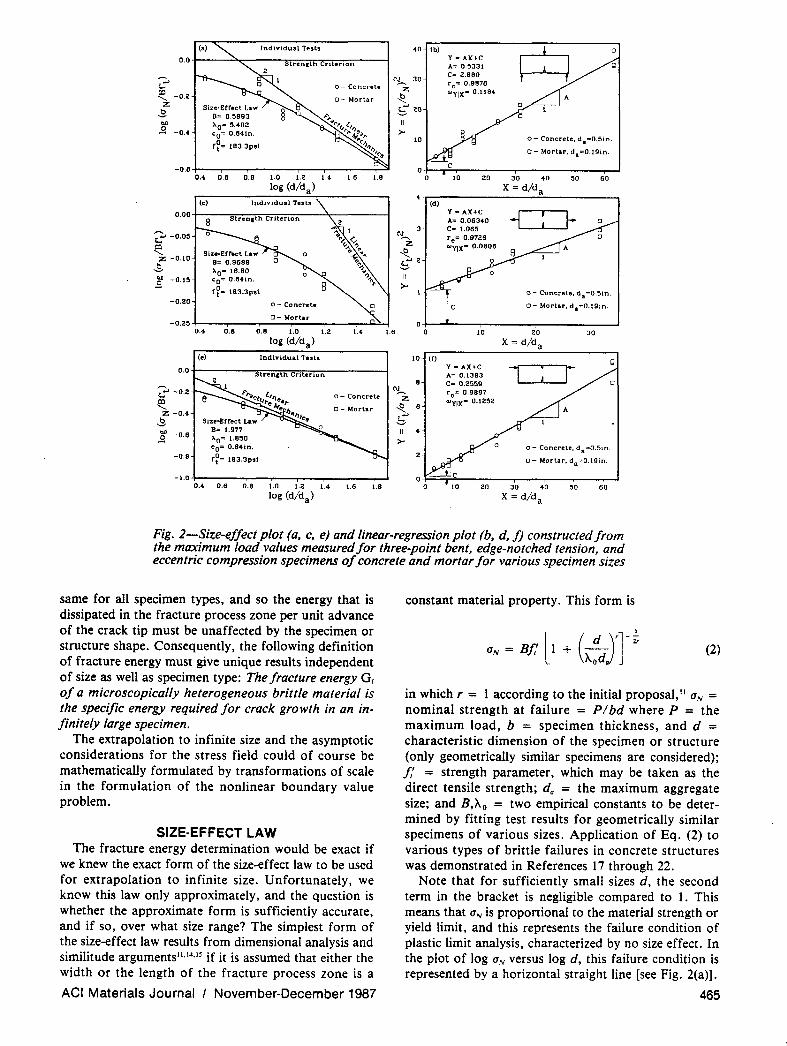
Fig. 2-Size-effect plot (a, c, e) and linear-regression plot (b, d, f) constructed from the maximum load values measured for three-point bent, edge-notched tension, and eccentric compression specimens of concrete and mortar for various specimen sizes
same for all specimen types, and so the energy that is dissipated in the fracture process zone per unit advance of the crack tip must be unaffected by the specimen or structure shape. Consequently, the following definition of fracture energy must give unique results independent of size as well as specimen type: The fracture energy Gr of a microscopically heterogeneous brittle material is the specific energy required for crack growth in an infinitely large specimen.
The extrapolation to infinite size and the asymptotic considerations for the stress field could of course be mathematically formulated by transformations of scale in the formulation of the nonlinear boundary value problem.
SIZE·EFFECT LAW The fracture energy determination would be exact if
we knew the exact form of the size-effect law to be used for extrapolation to infinite size. Unfortunately, we know this law only approximately, and the question is whether the approximate form is sufficiently accurate, and if so, over what size range? The simplest form of the size-effect law results from dimensional analysis and similitude argumentsll ,I4,IS if it is assumed that either the width or the length of the fracture process zone is a
ACI Materials Journal I November·December 1987
constant material property. This form is
[ ( d )r]- ~
UN = Bf: 1 + 'J\od. (2)
in which r = 1 according to the initial proposal, II UN = nominal strength at failure = Plbd where P = the maximum load, b = specimen thickness, and d = characteristic dimension of the specimen or structure (only geometrically similar specimens are considered); j,' = strength parameter, which may be taken as the direct tensile strength; da = the maximum aggregate size; and B,'J\o = two empirical constants to be determined by fitting test results for geometrically similar specimens of various sizes. Application of Eq. (2) to various types of brittle failures in concrete structures was demonstrated in References 17 through 22.
Note that for sufficiently small sizes d, the second term in the bracket is negligible compared to 1. This means that UN is proportional to the material strength or yield limit, and this represents the failure condition of plastic limit analysis, characterized by no size effect. In the plot of log UN versus log d, this failure condition is represented by a horizontal straight line [see Fig. 2(a)].
465
(0)
+ H r I -I>" I '~ ~(+)
Fig. 3-Specimen geometry and loading detail jor (a) three-point bent, (b) edge-notched tension, and (c) eccentric-compression specimens
As another limiting case when size d is extremely large, the number 1 in the bracket is negligible compared to the second term, and then UN is proportional to d- v,. This represents the strongest possible size effect and corresponds to the classical linear elastic fracture mechanics. In the plot of log UN versus log d, this limiting case projects itself as a straight line of downward slope - Y2. The plot of the size-effect law [Eq. (2)] consists of a gradual transition between these two limiting cases-plastic limit analysis for very small structures and lineF elastic fracture mechanics for very large structures. The limiting cases are known exactly, and the question is the shape of the transition, which is the purpose of Eq. (2).
The size-effect law in Eq. (2) results by dimensional analysis from the hypothesis that the total energy release W of the structure caused by fracture is a function of: (1) the length a of the fracture, and (2) the area nd. of the cracking zone, such that nd. = width of the front of the cracking zone = constant (d. = maximum aggregate size and n = 1 to 3 = empirical number). The original derivation II was simplified by truncation of the Taylor series expansion of a certain function. If this truncation is not made, a more general size-effect law is obtainedI2.1
'
in which B, Co, CI, Cz, ... , r = empirical constants. In practice, however, no case where this more general form would be needed has yet been found. It appears, and our analysis of test results will confirm it, that Eq. (2) can fit quite well any existing data with r = 1. The size range of the existing test data is at most 1: 10. Coefficient r might be needed for a broader size range, but this would be meaningful only if the statistical scatter were smaller than it normally is for concrete,
466
since otherwise coefficient r cannot be determined unambiguously. Note that Eq. (1) is valid only for r :::: 1; for other r, see the Appendix.
Scatter-free values of maximum loads for geometrically similar structures of different sizes can be generated with a finite element program based on fracture mechanics. In Reference 13 it was shown that for a certain r-value, Eq. (2) can fit such results even if the size range is as broad as 1:500. However, this range is much broader than feasible to test in a laboratory and needed in practice. Alternatively, scatter-free results can be calculated for the line crack model of Hillerborg if the method of Green's function is used (private communication by Planas and Elices, June 1986). Such calculations, as well as similar calculations made by Rots,27.28 Darwin, Hillerborg and others,26 show that the response in general, and the shape of the size-effect curve in particular, are sensitive to the precise shape of the softening stress-strain diagram or stress-displacement diagram. Various possible shapes of this diagram yield different extrapolations to infinite size. From the practical viewpoint, though, this fact does not seem to pose a serious problem. We do not need to extrapolate to infinity in the mathematically true' sense of the word. We need only to extrapolate to a specimen size that is sufficiently larger than the fracture process zone, and Eq. (1) seems sufficient for that.
Eq. (2), as well as Eq. (3), is valid for geometrically similar structures of specimens made of the same material. This implies the use of the same maximum aggregate size d •. When da is also variable, one needs to introduce the following adjustment of strength lw.26
(4)
in which fl and Co are empirical constants.
TEST RESULTS As already mentioned, the validity of fracture energy
determination through the size-effect law [Eq. (1)] requires that different types of specimens must yield roughly the same results if made from the same concrete. In the previous studyl6 where Of was first determined from the size effect, test results for only one specimen type-the three-point bent specimen-were used. Therefore, the testing has been expanded to include also other specimen types such as the doublenotched direct tension specimen sketched in Fig. 3(b) and the eccentric compression specimen shown in Fig. 3(c).
Fig. 3(d) shows the stress distribution across the ligament cross section drawn according to the bending theory. Although such stress distributions are unrealistic, they nevertheless reveal the great differences in the type of loading for the ligament cross section. For the notched tension specimen, the entire ligament is subjected to tension, which causes the fracture process zone to become very large. The opposite extreme is obtained for the eccentric compression specimen, for which the major part of the ligament is subjected to
ACI Materials Journal I November-December 1987
~omp'nsion a nd only. small p.n 10 I~n>;on IFi,. 3(d)!. In Ihis ~=. lit< <:OmfH"ts»on ahead of tho . ,ad th31 fom .. in tit< tensile zelne p,...-e"t, tM fraau~ proens wne from "",,ominl ,~ry la.lt". The bent specimen is a n'.dium Si, u' lion. in " 'hieh .ou,hl y half of the trOU 5«1;0" is ,ubj.cted 10 le"sion an d half '0 comp.e" ion, and Ihe fraClu •• proce", ,on, i, of medium , i,e.
Thul .... , .. that the choi.e of th."" three , >",cimen, co'·.rs ,he emi re broad ranliC of poSsibilil ies for the ,yflt of loadin, in Ihe lil a men, ero ...... ion. PIC,·i· ou.ly. ralhu diffuenl relul .. for Ihe fraClu te ."e' IY have been found for II>ese SpecirnfIU ... !>en ,Ite con,'enlion.;lI m ... ho,b ",-.crc used.
Phot<>(fllph. of tlte 1 .. 1 specim .... s ate .hown in Fig. 4(a). (b), and (0). Despi t. ,h. very diff"'nl Iyp<:> of loadini for Ihe ligament croSS section, i, ... as poMible to use spedmens of the same ,eo",clly e"ept for tI,e nOlchC!l. All the specimen, wcr. of [he same extcm ~1 .hape A, pr .. iously U.N in II sr..or f, acturo st udy.' Th. crOll setlioM of ,'''' specimens "'01. rC<"langular. aoo tM len,[ b"<Kiepih ralio was 8:l for all specim.n. (Fil. ll. Tl>c Cfoss ...... ionaJ hC"iShl$ of lhe specim.n. _.e d _. U. l. 6. and 12 in. (38.1, 76.2. 132.4. and JOoI.S mm) (see Fig. 3). The thic knell o f Ih. bendin, and comprC!lsion specim ..... was b .. I.S in. (38 mm) and !h'l of the t.nsion spc<:imcns b .. O.7S (19 mm), a$ shown in Fii. 3(1:» . For each Ipedme n .ize and . a"h t~po . thro. ,pecimen, were produced.
ThC!le three 'pe<:i.n." .. w<le from differe nt balCh .. ; however, from e:>c~ b~teh of COOCrCl. Or mon.r OM
specimen of each siu "':oJ ctit. N01C~ of dCplh d/ 6 and [hickn ... of 0.1 in. (2.S mm) (same .hickn ... fo, ,11 specimen sitts) " ...... cuI ..,i,h a diamond saw intO the ha.dmed specimens. The specim<IU ,,·.,.c ca. .. ,,·ith rite side of Mplh d in a ¥enkal poSil;o". n.. concrCle mix had a ",.t .. <emem rado of 0.6 and cemon, ·und· 1"'01 r.lio of 1:2:2 (.11 b~ ",eianl). The ma.<imUnI sr~v.1 si~. "'a$ d • .. O. S in . 02.7 mm). and the ma..i· mum la nd grain ,iz. w .. 0.19 in. (4.8J mm) . Mineral· olica lly. the aurOa-al. <o",is,ed of crushed limestone and siliceous ri,·u ",nd. Austill[. and ",nd "'Cle .ir· dried priof to mixi",. pOfdand ~menl C I~O, ASTM Type I. wilb no admixtures. """ used.
To ICI information on [M .freer of au!"C1"' •• iu," 1CC0nd "'-;cs of ,pecim~n. "'" mad<: of monar ..... hose w.t.r--cemem ""io "':oJ 0.$ .nd ~ment·sand .... Iio Wa\
1:2. Th.sam~ ,.nd .. for the co ncrete 'pe<:imcns ... u used w;lh lh. grav.1 ",nilled, ond 10 the maximum all' areaa[. size w",d • .. 0.19 in. (4. 83 mm) . nre water ... ·•· ment ,~,io di ffer.d from that for cOn, rett ,pecimens [0
:a<:hiove 'PPfo,imately tlte . amo wo. kability. To detClmine Ihe SlrOIli[h. com",,"ion cylinckrs of 3
in. diam.[er n 6 .2 mm) and 6 in . knllth (152.4 mm) ... ·cre caSt from cach batch of COncrc1e or monaro After ,h. Standard 28-day mOill curin •• the mean compr .. • ,ion Wtnlltk was /: _ 4865 psi OJ.S ~IPa) .... ·i,h a 5landard d •• iation (S.D.) _ SSO Pli 0.79 \ IPa) for the eoncr.te ,pecimens and 6910 pli ( ~7. 6 \IPa) with S.D. • "07 psi (1.43 ,\lPa) for the mOrtar ,pecim.n,. Each
ACI MaterialS Journal I No_ember·Oecember 1987
fi • . 4(o)-Th~'PO;nI ~nI sp«in~II Q/6-ill. (HZ'mm) f/fplh
of th ••• ,·.ht., was determined fmm thr.e cylind.r. for .ach ,pecimen lYpe I'ec T.b le 1) . The tensH. 5lren~t h wa, <"ima[e<! a.sj: _ 6.f.1{ I"i and Young's mod ul u, .. E, .. 57,000.;r; poi, with F. in psi ( I I"i - 689$ Pal.
The , pecimen ........ r.moved from tbe;r ply"'ood forms One d a )' aft.r Call1''l and ,,'.f< .ub'rquen[ly curod for T1 days (± I day) unlil,h. tQ[ in a mo;" room of 9:1 percent relalive humidity and 78 F O:S.6 C) temperatur •. AU tbe .pccimen . .... f. testod in a Io.ton (89.k N) [Fig . 4(b)! or 6O-Ion (S!4·I;N) [Fig. 4( d)!se",ocontrolled clo,ed.loop ).ITS [e" ing machine. The lab· Olalory cn"ironm ent l,.d a rela[ive humidity of oll<.>ul .. ,
Fir. 4(~)_£Nenlric.CQmpresslon loadinlS sp.:dml:l1 of 6-in. (lJl·mm) .uplll
6's Pf'"Ct"nt ~nd '~mJ>Cf1I'ur~ or ~I)out 78 F (25.6 C). and Ihe specimens w~re e~po$ed to Ibi. environmenl ap· pro. ima ldy three hour, b~for. Ihe . t3<1 of , h. ICIt.
Th. load ing for Ihe Ihr •• ·poin l ~nt sp«imens. as show" in Fig. 4{a l .• pplied Ih ree <Xl n,entra,ed loads on· to 'he .pocime n- one I()ad throlllln • hinge and two thr()~lh roU,,,. The "..,1 lurf'«1 ... cre ca",fully m.· ellint<:!.ro as to minimize the frklion of Ille '0Il .... The =entric compr ... i"" .peclm ..... wore loaded in a '..,r· tie:ll poIilion by t""O hing<$, a, .00 .. ,"" in FiS. 4{c). Tno loads .... er. applied Ihrou,h 11«1 plales 0.5 in. (1:.1 mm) Ihkk and gJUN 10 the "pe<imCII . For Ihe ecccn<ric comp, .. ,ion ,po,imen •. the load W", placed as <10K to Ihespecimen eorn er ~. fe~,iblc bu, "'" '0 d ose thaI Ihe spec im en wou ld rail by . hoorin g off it> torno r , alher
<e.
than by cn.ding frOm Ih. nOlch; by •• perimenlinl. the minimum """,i ble di".,,,,,, wa. found ' 0 b.< dIS ,
A sp.-oial lo"dinll , ri p was produced for tho tensile 5pe<imon, . It <Xlnsi" ed (Fill. 4(b) and 3(b)) ot" a icl of IwO aluminum pla,e. con,p .... ed toselher by I:>oIU. ShcOlJl of hard rubb.<r of I·m m thic~n<$$ ....... plal:ed bet ... ·«tIlhe sp«imen surf.~n and the plales t" dill rib· ul~ the clampinl .... 01Ily. The aluminum plat .. we", de· !i&ne<l so they could pro_ide , rips for the .pe<imo.., of all the . izes. For the lension specimen. 'he lar,o>1 ,;,e was om iuN. i.e., only ,peclm.n. of d _ 1.5, 3, .nd 6 in. (38.1. 76.2. and 152A mm) were used . A unlvcrY I joint \\,a. provid ed a, the top 3nd bottom connection, to the teSlilli machine to minimize in .plane and o ut·of. plonc hendill~ eff"",,,.
The .pecimen . we"" loadtd . , constant di .p laccmenl rate. For e~ch opc:cimc" lize lhe di.placemen, ~te " '1$
.. Ieeted to a chiev. t he maximum load in abou, ~ mint '" 30 sec).
ANALYSIS OF TEST RESULTS BY SIZE·EFFECT CAW
The les' r •• ul lS are ploued as Ihe square and drcu lar dala points ;n Fig. 2. The jlraph. o f log~, v."". 10il U. nond imenlion.li .cd " 'ith ... peet to J: and d •• • re on the left [Fig. 2(3), (e) •• nd (0)]. Al Ih. right (Ea:. lIb). (d), and lOt. the <arne lest result. are .ho..-n in linnr r..,..,..ion plou. based on the fact tha, Eq . (2) can boo alaebraically rurran;ed to. linear form. I""ead of Ih. plol Y _ A X .. C wllh X • d', Y _,,;~ . A _ C\V.)·· . C _ (B t: )·~. il i. mote conveni .... t to UloC the noodimeruional plot of Y' • A ' X ' + C" in which
Th. value of T _ I i, used in Fig. 2. If Eq _ (l) was fol. lowed ~ctly. the plot of Y' ,· ... u. X' ,houid be. uraiJIh' line of slope ,I ' at>d Y' .[nlO=t C ' (Fi,. 21. ... hi~h is why ,he dc~ia'ions hom Ihi, lide rep .. Knl Sllli"ical "'211". The plOI or Y' • ..,,-sus X' h.u 'he ad· vantage that one can apply linea. ".I["k.1 ,q;' <$$ion. yi<:td ina the .ize·effecl law IEq. (1) and (5)1 '$ the roafOss ion line. The ,·.rt ie.1 dc yia,ions from Iho reirel· si()n line may b. ~ha rn 'I ~r ll.~d by Ihc coeffi cie", of
ACI MaterialS Jou rnal I November·Decembe r 1987
Table 2-0ptimum values obtained by (a) linear regression and by (b) Levenberg-Marquardt algorithm
C, A, w. , -psi-' in. -. psi C/, W Y1X ,
, Wr'.n W" "'x, WO'
Loading Material x 10' x 10 ' Ib/in. 11,10 11,10 11,10 11,10 1110
a) Three-point bent Concrete 22.34 7.253 0.219 10.90 5.56 6.81 14.60 7.07
Table 3-Results of least-square optimization when specimens with concrete and mortar are analyzed simultaneously
Cf
Concrete, Loading C' A' Ib/in.
Three-point bent 2.880 0.5331 0.229
Notched tension 1.065 0.0634 0.210
Eccentric compression 0.2559 0.1383 0.233
variation WYIX and the correlation coefficient re, both indicated in Fig. 2. The value of A in Eq. (1) represents the slope of the regression line in the plot of Y = u:;/' versus X = dr, and from Eq. (5) it is readily found that A = A' /,' -2, d;;'.
By plotting the test results for concrete specimens and mortar specimens in the same diagram (Fig. 2), we are able to extend the size range of the data. Due to this fact, the plots are based on the generalized Eq. (2), which includes the effect of maximum aggregate size [Eq. (4)].
As for the value of exponent r, the overall optimum was found to be 0.954. However, for r = 1 the coefficient of variation of the deviations was only slightly larger. Therefore the value r = 1 is used for the sake of simplicity in all the plots as well as the numerical tables below.
Numerically, the test results are summarized in Tables 2 and 3. Tables 2(a) and (b) show the statistical results in which the concrete specimens and mortar specimens are treated separately, i.e., Eq. (2) is used without Eq. (4). Table 3 shows the statistical results when the data for all concrete as well as mortar specimens are treated collectively using both Eq. (2) and (4).
Table 2(a) shows the statistical results calculated separately for concrete specimens and mortar specimens
ACI Materials Journal I November-December 1987
Cf Mortar, w,"\ -Ib/in. wy,x w;'x W, W, We;
0.129 0.1184 0.0982 0.0338 0.1283 0.0537
0.118 0.0806' 0.0375 0.0597 0.1060 0.0728
0.132 0.1252 0.0844 0.0309 0.1356 0.0519
and also separately for each speCimen type. The optimization, based on linear regression, minimizes the sum EA(UN2
) where A stands for the difference between the measured value and the value according to the equation. The coefficient of variation of these deviations is WYIX' The table also lists the coefficient of variation w~x, which refers to the deviations in terms of UN'
Another possibility is to optimize the fit in terms of the deviations in UN, in which case the optimization problem is nonlinear. The fits, however, can be easily obtained with the standard computer library subroutine based on the Levenberg-Marquardt algorithm. The results are shown in Table 2(b).
The objective of our analysis is the value of Gf ,
which can ~e found by Eq. (1). Values of gf(cxO) for the present three-point bent, notched tension, and eccentric compression geometries are 6.37, 0.693, and 1.68, respectively, as calculated by linear elastic finite element analysis. The Ec value is listed in Table 1 for each loading case for concrete and mortar. The Gf values in Table 2(a) for concrete, i.e., 0.219, 0.205, and 0.2541bl in. (38.4, 35.9, and 44.5 N/m), show statistical scatter with a coefficient of variation of 11 percent. In Table 2(b), the resulting Gf values for concrete for the three specimen types are 0.192, 0.211, and 0.279Ib/in. (33.6, 37.0, and 48.9 N/m), and their coefficient of variation
469
Table 4-Measured maximum loads Maximum load P, Mean
12.0 2992 3010 3308 3103 Note: I Ib = 4.448 N; I m. = 25.4 mm.
is 20 percent. We see that the optimization by linear regression gives somewhat less scattered results, and therefore we will prefer it from now on.
It is hard to decide whether the differences in the Gj
values are purely random or whether they represent systematic differences between various specimen types. By extending the size range of the tests, random scatter can be minimized much more effectively than by increasing the number of specimens. Due to the cost of testing very large specimens, it has been decided to extend the size range in relative terms, Le., in terms of did., by analyzing simultaneously the results for concrete and mortar specimens. The results of such statistical analysis, based on minimizing again the sum I:A (q,v2), are shown in Table 3. In carrying out the statistical regression, parameter Co, governing solely the effect of aggregate size, has been required to be the same for all three specimen types; its value came out to be Co
= 0.64 in. (16.3 m). The coefficient of variation WY'X in Table 3 characterizes the deviations in terms of the variable Y' = [J,0 (1 + .j Col d.)1 aN ]2, and the coefficient of variation w~x characterizes the deviations in terms of the variable Y = aN' In the absence of a direct tensile test, the values of /" for concrete and mortar were estimated from the ACI formula /" :::};4 = 6JJ; where f: = average compressive strength = 4865 psi (33.5 MPa) and 6910 psi (1,120 MPa) for concrete and mortar, respectively. Then /,0 was determined so that the sum of squares of the difference of /,0 (1 + .jeold.) -f~ for concrete and mortar be minimized; this yielded J,D = 183.3 psi (1.26 MPa). Also, Ec was estimated for
470
concrete and mortar from ACl formula E, = 57,000 JJ; as 3976 ksi (27.4 MPa) and 4738 ksi (32.7 MPa), respectively.
The principal results in Table 3 are the Gf values. For concrete they are 0.229, 0.210, and 0.233 lb/in. (40.1, 36.8, and 40.8 N/m), which gives the coefficient of variation of 5.5 percent. We see that these results are indeed less scattered than those obtained for the size range of concrete specimens alone. For mortar, the Gj
values are 0.129, 0.118, and 0.132 lb/in. (22.6, 20.7, and 23.1 N/m), which give the coefficient of variation of 5.8 percent. Since the extension of the range of relative sizes reduces the relative scatter of results, it appears that the scatter is probably indeed of random origin, rather than due to omission of some unknown systematic influence, so the three types of specimens appear to give indeed approximately the same fracture energy value. This is of course to be expected theoretically, but only if the correct size-effect law is known. Thus we may conclude that Eq. (2) with Eq. (4), where r = 1, seems to be an acceptable approximate form of the size-effect law.
The measured maximum load values for all the individual specimens from which the present results were calculated are summarized in Table 4.
Our finding that the three fundamentally different specimen types yield roughly the same fracture energy is the principal result of the present study. Nevertheless, these results should eventually be subjected to a closer scrutiny using a much broader size range (much larger funds, of course, would also be needed).
It is interesting to determine the optimum fits of the data under the restriction that the Gj value be the same for all three specimen types. For this purpose, Eq. (1) with Gj from Eq. (2) may be algebraically rearranged to the linear plot
Y" = X"IGf + C" (6)
in which Y" = q,v2/gAcxo), X" = dlEc , and C" = CIgAcxo)(with r = I), Since for these variables the slope of the regression line is Gf-I (Fig. 5) and the fracture energy is a material constant independent of the specimen type, the test results for the three specimen types should be fitted by regression lines with arbitrary vertical intercepts but with the same slope. The test results have been analyzed collectively for all the specimen types under this restriction, and they are shown for concrete and mortar in Fig. 5(a) and (b). Due to the scatter of the test data apparent in these figures, we cannot say that the test results prove that the slope (and thus the fracture energy) is the same for all the three specimen types; however, we must also admit that these plots do not reveal any systematic deviation from the constant common slope Gj I. To illustrate the scatter more clearly we may shift the data for each specimen type vertically so that the regression lines coincide (the shift being indicated by the vertical intercepts C, for specimen types i = 1, 2, 3). The resulting plot is shown in Fig. 5(c) and (d) for concrete and mortar, and it is
Fig. 5-Plots demonstrating independence of fracture energy from specimen type, (a, c) concrete and (b, d) mortar
seen again that although the large scatter prevents us from concluding that all three specimen types yield the same slope, no systematic deviations from a common slope are apparent.
Comparing the size-effect plots in Fig. 2(a), (c), and (e), we may note that in the case of the eccentric compression specimen the curve is quite close to the .. asymptote of slope - Yz for linear elastic fracture mechanics, while for the case of tension specimen the curve is quite remote from this asymptote, and for the three-point bent specimen an intermediate situation occurs. From comparisons of these graphs, we may observe that the size range of the tension specimens would have to be increased about 20 times to approach the asymptote as closely as the compression specimen. Obviously, the tension specimen is by far the best for exploring, with relatively small specimen sizes, the behavior near the horizontal asymptote for the strength criterion, and the eccentric compression specimen is best for finding the linear fracture mechanics asymptote, and through it the value of Of. What is the reason for these differences in behavior?
It is the difference in the size of the fracture process zone that causes these behavioral differences, as we will demonstrate by simplified analysis as well as finite elements. The difference can be understood intuitively by considering (according to the bending theory) linearized stress distributions across the ligament as shown in Fig. 3(d). Even though these stress distributions are no doubt far from the real ones, they make it clear that for the eccentric compression specimen the crack as it extends from the tension notch soon runs into a compression zone, and so the fracture process zone for the eccentric compression specimen can occupy only a small fraction of the ligament. The smaller the relative size of the fracture process zone, the closer the behavior
ACI Materials Journal I November-December 1987
. should be to the limit of linear elastic fracture mechan-ics. For the tension specimen, on the other hand, the entire ligament is under tensile stress, and so nothing prevents the fracture process zone from being as long as the entire ligament itself. For such a large fracture process zone, the behavior should be close to the strength criterion limit, as corroborated by Fig. 2(c). For the three-point bent specimen, the size of the fracture process zone is also limited by the compression field of the top side of the ligament [Fig. 3(d)], but the tension part of the ligament is larger than it is for the eccentric compression specimen, and so the fracture process zone should be of medium length. This explains why the sizeeffect plots for this type of specimens are intermediate between the tension and eccentric compression specimens of the same exterior dimensions.
It must be emphasized that the size-effect method fails if the size range is insufficient compared to the width of the scatter band of the test results. The relevant data scatter is characterized by the standard deviation A of the regression line slope A and the corresponding coefficient of variation WA> which are defined as
(7)
where n is the number of all the data points in the linear regression, s< is the coefficient of variation of the X values for all the points, and Sy!X is the standard deviation of the vertical deviations from the regression line. The values of WA are listed in Tables 2 and 3.
If the size range were so narrow that it would be approximately equal to the width of the scatter band, the data points would fill roughly a circular region (Fig. 6). One could still obtain a unique regression line, but its
471
y (a) y (b) Y (e) / 0
o~ A o 0
_0 80 o 0- --=t....
0 0 0
A 0 0
/ No! O.K. O.K
X X X
Fig. 6-(a) Size-effect method is inapplicable when the size range is too small compared to scatter; (b, c) size range is sufficient
slope would be highly uncertain and could even come out negative. To prevent this from happening, it is necessary that the value of "'A would not exceed about 0.1. Even then, by testing very many specimens (large n) one could make "'A sufficiently low even when the data points fiII roughly a circular region rather than an elongated band. To prevent this from happening, one needs to require further that, for any n, the value of "'l1xl",x would not exceed about 0.15.
Obviously, if the test results are consistent, with a low scatter, one can do with a narrower size range than if the test results are highly scattered.
From "'A one can approximately estimate the coefficient of variation "'0, of the fracture energy Gj == gAcxo)/ AEe• If Gj is assumed to be perfectly correlated to Ee , then "'Of = "'A' If Gf is assumed to be uncorrelated to Ee then, as a second-order approximation, "'Of = "'0 where ",b = "'~ + "'} and "'E is the coefficient of variation of Ee. In reality one may expect "'A ~ "'Of ~ "'0'
It needs to be pointed out also that the size-effect approach can be destroyed by other size effects. Theymay arise from diffusion phenomena, e.g., the heating (and microcracking) caused by hydration heat, which may be significant for very large specimens, or the drying of the specimen, which is more severe for thinner or smaller specimens.
BRITTLENESS NUMBER Our finding that the size-effect law yields approxi
mately unique Gj values regardless of size and geometry makes it meaningful to base on this law a. nondimensional characteristiclS,30 that indicates whether the behavior of a given specimen or structure is closer to limit analysis or to linear elastic fracture mechanics. The relative structure size ~ = did. cannot serve as an objective indicator of this behavior. This is clear from the present tests. For ~ = 4, e.g., the behavior of the tensile specimen is (according to Fig. 2) closer to plastic limit analysis based on the tensile strength, while the behavior of the eccentric compression specimen for ~ == 4 is closer to linear elastic fracture mechanics. An objective indicator is the recently proposed Bazant'sll,JO brittleness number /3. It is defined as
472
(8)
and can be calculated after ~o has been determined either experimentally or by finite element analysis. The value of (3 == 1 indicates the relative size did at the point where the horizontal asymptote for the ;trength criterion intersects the inclined straight-line asymptote for the energy failure criterion of linear elastic fracture mechanics (Fig. 2). So /3 == 1 represents the center of the transition between these two elementary failure criteria.
For /3 < 1, the behavior is closer to plastic limit analysis, and for /3 > 1 it is closer to linear elastic fracture mechanics. For (3 ~ 0.1, the plastic limit analysis may be used as an approximation, and for /3 ~ 10, linear elastic fracture mechanics may be used as an approximation. For 0.1 < /3 < 10, nonlinear fracture analysis must be used.
To find the brittleness number, one needs to calculate the coefficient Ao, which represents the value of did. at the point of intersection of the horizontal straight line and the inclined straight line in Fig. 2. The inclined straight line is given by the equation UN = [GjElgj(cxo)d)'\ which is valid according to linear elastic fracture mechanics for any two-dimensional structure. The horizontal line is given by the equation UN == Bf: when coefficient B is obtained by plastic limit analysis. By equating both expressions for UN' BaZantJ1
obtained the following expressions for the transition value do of the characteristic dimension d of the structure and of the corresponding transition value of the relative structure size did.
(9)
Therefore31
(10)
Practical calculations may generally proceed as follows: First solve the structure by plastic limit analysis,
ACI Materials Journal/November-December 1987
which yields the value of B. Second, solve the structure by linear elastic fracture mechanics, which yields the value of g,. Third, calculate {3 from Eq. (10). This method of calculating {3 requires no laboratory tests. Alternatively of course, the brittleness number of a certain type of structure of a given size can be determined by fitting the size-effect law either to test results or to finite element results for ultimate loads of structures of similar geometry but sizes that differ from the given size. (These finite element results must be based on a softening stress-strain or stress-displacement relation.)
It must be emphasized that the value of B must be calculated by plastic limit analysis rather than an allowable elastic stress formula. For example, for an unreinforced beam of span L, rectangular cross section of width b and net depth d in the middle, with concentrated load P at midspan, we have M~ = PL/4 = /" bd2/4 = plastic ultimate bending moment at midspan. From this we get UN = Plbd =/,' dlL or UN =BI: where B = dlL = constant (for geometrically similar beams). It would be of course incorrect to use the elastic formula M~ = I: bd2/6 which would yield B = 2d/ 3L.
The brittleness number can serve as a basic qualitative indicator of the type of response. In this sense it is in fact analogous to the nondimensional characteristics used, e.g., in fluid mechanics, such as the Reynolds number.
Some re~archers have tried to characterize the effects of structure size on the qualitative fracture behavior by means of some nondimensional combination of 0" /,', and Ec. This is, however, insufficient because these parameters cannot reflect differences in structure geometry. For example, CarpinterP2 characterized the effect of structure size on its brittleness by the nondimensional ratio s = 0/ b I: and Hillerborg2l by the nondimensional ratio of some structural dimension to the characteristic length Ich = Ec all,'2, defined in the same manner as the size of the small-scale yielding zone in metals. 8
•23 However, these nondimensional ratios,
i.e., the Carpinteri's and Hillerborg's brittleness numbers, are objective only for comparisons of different sizes of structures of the same geometry. For the same value of either Carpinteri's or Hillerborg's brittleness number, the failure of a structure of one geometry can be quite brittle, i.e., close to linear elastic fracture mechanics, while the failure of a structure of another geometry can be quite ductile, i.e., close to limit analysis.
The effect of structure size on the brittleness of its response is manifested not only in the maximum load but also in the post-peak shape of the load-deflection diagram. As graphically illustrated in Fig. 6 of Reference 15, the total deflection is a sum of the deflections due to the fracture process zone and to elastic strains. As the size is increased, the former remains about the same while the latter increases, causing the post-peak diagram to become steeper and steeper and eventually reverse to a snapback-type load-deflection diagram that . is unstable under both load and displacement controls.
ACI Materials Journal I November-December 1987
R·CURVES FOR DIFFERENT SPECIMEN TYPES According to classical linear elastic fracture mechan
ics, the specific energy required for crack growth R is constant and equal to the fracture energy 0,. For materials that do not follow linear elastic fracture mechanics, R varies with the length of crack extension from the notch. This variation is described by the socalled resistance or R-curve. When the R-curves were first observed for ductile fracture of metals, it was proposed33.34 that the shape of the R-curve may be considered to be approximately a material property. For concrete, this concept was introduced by Wecharatana and Shah,3l and further refined by Bazant and Cedolin.36 Analysis of extensive test data from the literature showed that, as a crude approximation, the R-curve may be considered unique for a certain limited range of specimen geometries,36 but it can be very different for some very different specimen geometries. 16 Nevertheless, even though the R-curve is not a unique material property in general, it represents a simple, convenient way to reduce nonlinear fracture analysis to a linear one.
For a specified specimen geometry and type of load. ing, there is a one-to-one relatio,nship between the sizeeffect law and the R-curve. 16 If one is known, the other can be easily calculated. The method described previouslyl6 has been used to calculate the corresponding R-curves from the size-effect curves in Fig. 2. They are shown in Fig. 7. Fig. 7(a) and (c) give the plots of the specifia energy required for crack growth R as a functio'n of the crack length c measured from the notch. Fig. 7(b) and (d) show (for the same crack lengths c) the relative values defined as R for the given specimen divided by R for the three-point bent specimen taken as a reference (by definition, for the threepoint bent specimen the relative values are all 1).
From Fig. 7 we may observe that for the three-point bent specimens and the eccentric compression specimens the R-curves are not too far apart. Therefore, their mean could be used as a material property for a crude approximation. For the tension specimen, however, the R-curve is very different. This proves that in general the R-curve of concrete cannot be considered to be a unique material property. This conclusion, however, does not apply to the asymptotic values.
The asymptotic value of the R-curve (c-+oo) corresponds to the limiting case of elastic fracture mechanics and is determined by the straight-line asymptote of slope - Y2 in Fig. 2. While the R-curves are very different for small crack lengths, the asymptotic values are nearly the same, up to a reasonable scatter range that is inevitable for a material such as concrete. This conclusion, which is particularly conspicuous from the relative curves in Fig. 7(b) and (d), is a basic result of this study. Since the final asymptotic value of the R-curve represents the fracture energy 0, as defined in this paper, this conclusion agrees with the previous conclusion that the fracture energies are approximately the same for various specimen types, with a reasonable scatter that appears to be random rather than systematic.
473
0.3~-------------' (al
~ 0.2 It! ........................ : ... . ~ 0.1 I .. / .. , .... a: t.,., .... " •••• - Gr = 0229 Ih 1m • R(c)3PB
•..•. Gr = 0 ZlO Ib lin. R(c)NT
...... d
'" .c .:::. S c::
_. Gr = 0.233 Ib./In .. R(c)EC O.O-f----r---i----.---'---i
Fig. 7-R-curves for three-point bent, edge-notched tension, and eccentriccompression specimens of (a) concrete and (c) mortar, and (b, d) relative R-curves
~:"':-----T---}With
without
size-effect law
c, Crack Length
Fig. 8-Extrapolation of R-curves with and without size-effect law
With the help of the R-curves it may be explained why the methods currently used to define and measure the fracture energy do not lead to unique results and exhibit a large spurious dependence on the specimen size. These existing methods generally use the same specimen geometry and dimensions (size) and rely on measurements at various crack lengths or notch lengths. The work of fracture method recently adopted by RILEM2s is of that type, as is the ASTM method for the measurement of R-curve. Because the specimens are of one size, the results correspond to a short segment of the size-effect curve, which in turn corresponds to a relatively short segment of the R-curve. This is so, even if the measurements are done at various crack lengths or various notch lengths, as demonstrated by finite element results in Fig. 7 of Reference 16. Thus one obtains for the R-curve a set of measured points occupying only a small part of the R-curve, as illustrated in Fig. 8. Obviously, extrapolation to c- 00 from such data for a limited size range is ambiguous. Due to in-
474
evitable statistical scatter, the extrapolated dashed or solid curves in Fig. 8 yield almost equally good fits of the measured data. It must be concluded that the existing methods that do not use specimens of very different sizes are inherently incapable of giving consistent results for the fracture energy as defined here. They yield fracture energy values illustrated by the asymptote of the dashed curves in Fig. 8, which are usable in the analysis of structures that are not much larger than the specimens tested, but are inapplicable to structures that are much larger.
These difficulties in determination of R-curve from scattered data for a limited size range are further compounded by the fact that the R-curve has to be determined as an envelope of a family of fracture equilibrium curves. 16
,36 When these curves are scattered, an envelope simply cannot be constructed. 16
FINITE ELEMENT ANALYSIS OF TEST RESULTS The size effect in fracture can also be described by
finite elements. 16,37 By optimizing the material fracture
parameters so as to obtain the finite element fit of the present test data, it is possible to obtain the fracture energy_ Is this result approximately the same as the fracture energy value obtained directly from the sizeeffect law?
To answer this question, the present test specimens were analyzed by finite elements in exactly the same manner as described on pages 302 to 303 of Reference 16. The analysis utilizes the crack band model with a square mesh of four-node quadrilateral elements in the fracture region. The fracture is simulated by a band of cracking elements of a single-element width. The cracking is described by gradual strain-softening in the elements of the crack band. To explore the effect of the shape of the stress-strain diagram for strain softening in
ACI Materials Journal I November-December 1987
the crack band, the analyses are carried out both for linear softening [Fig. 9(a)], as in Reference 37, and for strain-softening given as an exponential passing through the same peak point [Fig. 9(b)]. The fracture energy in this approach is given by the area under the uniaxial tensile stress-strain diagram, multiplied by the width We
of the crack band front. This width must be considered to be a material property independent of the element size and represents a certain small multiple of the aggregate size. The finite element solutions are obtained by step-by-step loading. They yield the maximum loads to which the size-effect law can be matched.
The results of the finite element calculations are compared with the direct analysis of test data by the size-effect law in Table 5 and Fig. 10. The size-effect law results are listed in the first column for Gf in Table 5. The finite element results obtained with linear and exponential strain-softening are listed in the last two columns of Table 5. These values were obtained by fitting the size-effect law to the finite element results for specimens of various sizes, and then matching the sizeeffect law to the curve [Eq. (2)] that optimally describes the test data. The fracture energy may then be obtained either from the asymptotic slope for the sizeeffect curve that fits the finite element results (Table 5), or directly from the area under the stress-strain curve (Fig. 9) considered in the finite element analysis, times width We (Table 6). For the three types of specimens used, the results are given in the last two columns of Table 5, separately for concrete and mortar. Since all the specimens were cast from the same concrete, the Gf values from finite elements with linear softening were forced to be the same for all the three types of tests (0.230 lb/in. or 40.3 N/m). The exponential softening is always introduced in such a manner that the areas under the stress-strain diagram, and thus also Gf , would be the same as for linear strain softening. The results for exponential strain softening (material parameters given in Table 6) are different, but only marginally so, and are close to the Gf values calculated directly from the size-effect law for each specimen type - for concrete as well as mortar. Compare the columns of Table 5.
Generally, the finite element calculations indicate relatively good agreement between the Gf values that give optimum fits of the measured maximum loads by the finite element program and those obtained by fitting the size-effect law to the measured maximum loads for various specimen sizes. The finite element results in Fig. 10 are compared directly with the test data and the size-effect law fits from Fig. 2 based on both the log (aNI!,') versus log (did.) plot (a, c, and e) and the linear regression plot (b, d, and f). The finite element meshes used to obtain these results are drawn in Fig. 11. The coefficient of variation WYIX for the linear regression plots is given for each loading case and for both linear and exponential softening. Among these fits, the best that one could hope to obtain is the sizeeffect law, which has an average coefficient of variation of wYlx = 0.11 where wYlX = {[w2
Y1X (3PB) + w~ IX
(ND + w~x (EC)]!3} 112; 3PB, NT, and EC stand for
ACI Materials Journal I November-December 1987
(0)
(b)
f' t
€
-o€ a = C e (softening)
f' C = _t_
-o€ e
0= Gf
we
f' t f'2 t
2 Ee
Fig. 9-Uniaxial stress-strain curves for (a) linear and (b) exponential softening
Table 5-Comparison of fracture energy from size-effect law and finite element results
Size-effect Linear Exponential
law 0/, softening softening Loading Material Ib/in. O/,Ib/in. O/,Ib/in.
the three-point bent, notched tension, and eccentric compression specimens, respectively. For linear softening WYlX = 0.14 and for exponential softening wYIX = 0.20. Linear softening seems to match the test data somewhat better than exponential softening, for this particular set of data.
The finite element crack band model can also be used to obtain the R-curves. 16
•37 The results of such calcula
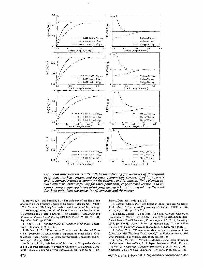
tions are shown in Fig. 12. The finite element R-curves obtained for both linear and exponential softening follow the general trend of the R-curves obtained by the size-effect law from the measured maximum loads (Fig. 7). The linear softening seems to give a slightly better agreement than the exponential softening when compared to the R-curves deduced directly from the test data.
475
-0.3
~
~ 'Z -0.0
..3-.. o
- -0.7
(a) 0- Concrete
a - Mortar
-- Size-Effect Law ••• _- F.E.M. Linear Softening -. F.E.N. Exponential Softemng
Fig. lO-Comparison of finite element results for three-point bent, edge-notched tension, and eccentric-compression specimens in (a, c, e) size-effect plot and (b, d, f) linear regression plot
SHEAR FRACTURE (MODE II) All of our analysis thus far dealt with the opening
fracture mode (Mode I). According to test results in a recent paper, 29 the size-effect law is also applicable to shear fracture (Mode II). Shear fracture can be produced on the same specimen as used here for tension and compression, although with a different type of loading, shown in Reference 29. For this loading the fracture energy for Mode II can be calculated from Eq. (I) using gf (ao) = 2.93, as indicated by linear elastic fracture mechanics. 8
,23,24 In finite element modeling, the crack band model is applicable to shear fracture as well, provided the smeared cracks within the finite elements are allowed to be inclined with regard to the crack band, letting them form with the orientation normal to the maximum principal stress. The compression stiffness and strain-softening of the concrete between the cracks, loaded in the direction parallel to the cracks, is taken into account. 29
Tests for shear fracture, comparable with the preceding results, were conducted with the same type of concrete. Therefore, the results for shear fracture are also listed in Tables 7 and 8. The Mode II fracture energy GV is found to be far larger than the Mode I frac-
476
ture energy Gf = Gj. This may be explained by compressional resistance to conCI<ete between the cracks in the inclined direction parallel(,to the cracks. 29 The sizeeffect regression plots for Mode II are shown in Fig. 13(a) and (b) and the finite eleinent results in Fig. 13(c) and (d).
Recently, Bazant and Prat38 applied the size-effect law to Mode III fracture tests of cylindrical specimens with circumferential notches, subjected to torsion, and used again Eq. (1) to determine the Mode III fracture energy of concrete.
CONCLUSIONS 1. Fracture energy of a brittle heterogeneous mate
rial such as concrete may be defined as the specific energy required for fracture growth when the specimen or structure size tends to infinity. In this definition the fracture energy is a unique material property, independent of specimen size, shape, and type of loading.
2. The foregoing definition reduces the problem to the question as to which form of the size-effect law should be used for extrapolating the test results to infinite size. Although the exact size-effect law is not known, the present test results indicate that Bazant's
ACI Materials Journal I November-December 1987
approximate size-effect law [Eq. (2)], with a correction for the maximum aggregate size [Eq. (4)], may be acceptable for practical purposes.
3. When the present method is used, different types of fracture specimens - such as the edge-notched tension specimen, three-point bent specimen, and notched eccentric compression specimen - yield approximately the same values of fracture energy. The observed scatter range is about the same as the usual range of inevitable scatter for concrete. Thus, the present method of defining and measuring the fracture energy appears to be approximately independent of both the specimen size and type - a goal not yet achieved with other methods.
4. Bazant'sIS.30 brittleness number {3 [Eq. (8) and (10)], based on the size-effect law, may be used as a nondimensional characteristic of fracture similitude, which indicates how close the structure behavior is to linear elastic fracture mechanics or to limit analysis. Bazant's brittleness number, in contrast to Carpinteri's or Hillerborg's, is independent of the shape of specimen or structure, and so it can be used to compare the brittleness of structures of different shapes. For {3 ~ 0.1, the response of a structure of any shape is essentially ductile and plastic limit analysis applies, for {3 ;;?: 10 it is essentially brittle and obeys linear elastic fracture mechanics, and for 0.1 < {3 < 10 the brittle and ductile responses mix and a nonlinear fracture analysis is required.
5. R-curves for various specimen types, calculated on the basis of the size effect from the maximum loads of specimens of different sizes, are very different for short crack lengths but approach a common asymptotic value for large crack lengths.
6. The present test results can be described by the finite element crack band model. The fracture energy values determined from the size effect approximately agree with the fracture energy value. used in the finite element code, which represents the area under the tensile stress-strain diagram multiplied by the width of the cracking element at fracture fronL
ACKNOWLEDGMENTS Partial financial support under Air Force Office of Scientific Re
search Grant No. 83-00092 and contract No. F49620-87-C-00300EF with Northwestern University is gratefully acknowledged.
Further financial support has been obtained under a cooperative research program with Universidad Politecnica de Madrid, funded under U.S.-Spanish Treaty (Grant CCA-8309071.)
REFERENCES 1. Shah, S. P., Editor, Application of Fracture Mechanics to Ce
mentitious Composites, Martinus Nijhoff Publishers, Dordrecht, 1985, 714 pp.
2. Bazant, Z. P.; Kim, J. K.; and Pfeiffer, P., "Determination of Nonlinear Fracture Parameters from Size Effect Tests," NATO Advanced Research Workshop on Application of Fracture Mechanics to Cementitious Composites," Northwestern University, Evanston, Sept. 1984, pp. 143-169.
ACI Materials Journal I November-December 1987
(e)
~~. "-~
!.-- d -I
(g)
l-2d
I -'-
-! l--wc :d/~2
(i)
4d
1 Fig. lI-Finite element meshes jor (a, b, c) three-point bent, (d, e, f) edge-notched tension, and (g, h. i) eccentric-compression specimens
Table 7 -Comparison of fracture energy from size-effect law and finite element results for shear fracture
Size-effect Linear Exponential law softening softening
3. Wittmann, F. H., Editor, "Fracture Toughness and Fracture Energy of Concrete," Proceedings, RILEM International Conference on Fracture Mechanics of Concrete, EPFL, (held in Lausanne, 1985), Elsevier, Amsterdam, 1986,699 pp.
4. RILEM Committee 50-FMC, "Determination of the Fracture Energy of Mortar and Concrete by Means of Three-Point Bend Tests on Notched Beams," RILEM Draft Recommendation, Materials and Structures, Research and Testing (RILEM, Paris), V. 18, No. 106, July-Aug. 1985, pp. 285-290.
5. Hilsdorf, H. K., and Brameshuber, W., "Size Effects in the Experimental Determination of Fracture Mechanics Parameters," Application of Fracture Mechanics to Cementitious CompOsites, Martinus Nijhoff Publishers, Dordrecht, 1985, pp. 361-397.
477
~
c::
" ..ci 0
~ a:
~
c::
" g $ a:
~
c::
" ..ci 0
$ a:
~
c::
" g $ a:
0.3 T':""(a):----------------,
0.2
0.1 ~ ....... .
I / ....... .
1"".:"//" .... --- Gr = 0230 Ib lin, R(c)3PO
Gr = 0230 Ib lin , R(c)NT
- Gr = 01230 Ib 1m, R(C)cC 0.0+----.,........---~ __ __,--...::..:.--1
0.0 0.5 1.0 1.5 2.0
Crack Length, c (in.) O.l~-r.-(C"':")--------------,
0.10
O.O~
--- Gr = 0.130 Ib./in., R(c)3PB
--.-- Gf = 0.130 lb./tn., R(c)NT
-' Gr = 0.130 Ib./in .. R(c)EC 0.00+----....,..--:.-:.-..-___ ..,.....::.:.-'
0.0 0.2 0.4 O.B
Crack Length. c (in.) 0.3-r.-(e"':")--------------,
0.2
0.1
-.-.-.--:::------..,..,.,~--I ~- .... .. '
..-
"',
.. ,"/."/.,
.' -- Gr =- O.Z49 lb./in., R(c)3PB
••••• Gr = 0.249 Ib./in., R(C)NT
-. Gr = 0.249 Ib·/tn .• R(c)EC 0.0+---....,.---.,........:...--....,..---.,.::..::.--1
Fig. 12-Finite element results with linear softening for R-curves of three-point bent, edge-notched tension, and eccentric-compression specimens of (a) concrete and (c) mortar; relative R-curves for (b) concrete and (d) mortar; finite element results with exponential softening for three-point bent, edge-notched tension, and eccentric compression specimens of (e) concrete and (g) mortar; and relative R-curves for three-point bent specimens for (f) concrete and (h) mortar
6. Horwath, R., and Persson, T., "The Influence of the Size of the Specimen on the Fracture Energy of Concrete," Report No. TVBM· 5005, Division of Building Materials, Lund Institute of Technology.
7. Hillerborg, Arne, "Results of Three Comparative Test Series for Determining the Fracture Energy Gf of Concrete," Materials and Structures, Research and Testing (RILEM, Paris), V. 18, No. 107, Sept.·Oct. 1985, pp 407·413.
9. Bazant, Z. P., "Fracture in Concrete and Reinforced Con· crete," Pre prints, IUTAM Prager Symposium on Mechanics of Geomaterials: Rocks, Concretes, Soils, Northwestern University, Evans· ton, Sept. 1983, pp. 281·316.
10. Bazant, Z. P., "Mechanics of Fracture and Progressive Crack· ing in Concrete Structures," Fracture Mechanics oj Concrete: Struc· tural Application and Numerical Calculation, Martinus Nijhoff Pub·
478
lishers, Dordrecht. 1985, pp. 1·93. 11. Bazant, Zdenek P., "Size Effect in Blunt Fracture: Concrete,
Rock, Metal," Journal of Engineering Mechanics, ASCE, V. 110, No.4, Apr. 1984, pp. 518-535.
12. Bazant, Zdenek P., and Kim, Jin·Keun, Authors' Closure to Discussion of "Size Effect in Shear Failure of Longitudinally Reinforced Beams," ACI JOURNAL, Proceedings V. 82, No.4, July·Aug. 1985, pp. 579-583. Also, "Effects of Aggregate and Structure Sizes on Concrete Failure," correspondence to J. K. Kim, May 1985.
13. Bazant, Z. P., "Comment on Hillerborg's Comparison of Size Effect Law with Fictitious Crack Model," dei Poli Anniversary Vol· ume, Politecnico di Milano, Oct. 1985, pp. 335·338.
14. Bazant, Zdenek P., "Fracture Mechanics and Strain·Softening of Concrete," Proceedings, U .S.·Japan Seminar on Finite Element Analysis of Reinforced Concrete Structures (Tokyo, May, (985), American Society of Civil Engineers, New York, 1986, pp. 121·150.
Fig. 13-(a) Size-effect plot, (b) linear-regression plot constructed from maximum load values measured for shear fracture specimens of concrete and mortar, for various specimen sizes, and (c) finite-element results in size-effect plot, (d) linear-regression plot
15. Bdant, Z. P., "Fracture Energy of Heterogeneous Material and Similitude," Pre prints, RILEM-SEM International Conference on Fracture of Concrete and Rock (Houston, June 1987), Society for Experimental Mechanics, Bethel, pp. 390-402.
16. Balant, Zdenek P.; and Kim, Jin-Keun; and Pfeiffer, Phillip A., "Nonlinear Fracture Properties from Size Effect Tests," Journal oj Structural Engineering, ASCE, V. 112, No.2, Feb. 1986, pp. 289-307.
17. Batant, Zdenek P., and Kim, Jin-Keun, "Size Effect in Shear Failure of Longitudinally Reinforced Beams," ACI JOURNAL, Proceedings V. 81, No.5, Sept.-Oct. 1984, pp. 456-468.
18. Batant, Zdenek P., and Cao, Zhiping, "Size Effect in Shear Failure of Prestressed Concrete Beams," ACI JOURNAL, Proceedings V. 83, No.2, Mar.-Apr. 1986, pp. 260-268.
19. Batant, Zdenek P., and Cao, Zhiping, "Size Effect in Brittle Failure of Unrein forced Pipes," ACI JOURNAL, Proceedings V. 83, No.3, May-June 1986, pp. 369-373.
20. Batant, Zdenek P., and Cao, Zhiping, "Size Effect in Punching Shear Failure of Slabs," Report No. 85-8/428s, Center for Concrete and Oeomaterials, Northwestern University, Evanston, May 1985. Also, ACI Structural Journal, V. 84, No. I, Jan.-Feb. 1987, pp. 44-53.
21. Batant, Z. P., and Sener, S., "Size Effect in Torsional Failure of Longitudinally Reinforced Concrete Beams," Journal oj Structural Engineering, ASCE, V. 113, No. 10, Oct. 1987, pp. 2125-2136.
22. Bdant, Z. P.; Sener, S.; and Prat, P. C., "Size Effect Tests of Torsional Failure of Concrete Beams," Report No. 86-12/428s, Center for Concrete and Geomaterials, Northwestern University, Evanston, Dec. 1986, 18 pp.
23. Broek, D., Elementary Engineering Fracture Mechanics, Sijthoff and Noordnoff International Publishers, Leyden, 1978,408 pp.
24. Tada, H.; Paris, P. C.; and Irwin, O. R., The Stress Analysis oj Cracks Handbook, 2nd Edition, Paris Productions, Inc., St. Louis, Mo. 1985.
25. Hillerborg, A., "The Theoretical Basis of a Method to Determine the Fracture Energy Gr of Concrete," Materials and Structures. Research and Testing (RILEM, Paris), V. 18, No. 106, July-Aug. 1985, pp. 291-296.
ACI Materials Journal I November·December 1987
26. Balant, Z. P., "Mechanics of Distributed Cracking," Applied Mechanics Reviews. V. 39. No.5. May 1986. pp. 675-705.
27. Rots. J. G.; Nauta, P.; Kusters, G. M. A.; and Blaauwen· draad, J., "Smeared Crack Approach and Fracture Localization in Concrete," Heron (Delft), V. 30, No. I, 1985.48 pp.
28. Rots, J. G., "Strain·Softening Analysis of Concrete Fracture Specimens," Proceedings, RILEM International Conference on Fracture Mechanics of Concrete, EPFL, Lausanne, 1985, pp. 115-126.
29. Batant, Z. P., and Pfeiffer, P. A .• "Shear Fracture Tests of Concrete," Materials and Structures. Research and Testing (RILEM, Paris), V. 19, No. 110, Mar.·Apr. 1986, pp. 111-121.
30. Batant, Z. P., Seminar, Rensselaer Polytechnic Institute, Troy, Jan. 31, 1986.
32. Carpinteri, A., "Notch Sensitivity in Fracture Testing of Ag· gregative Materials," Engineering Fracture Mechanics, V. 16, 1982, pp.467-481.
33. Irwin, O. R., "Fracture Testing of High Strength Sheet Mate· rial," ASTM Bulletin. Jan. 1960, p. 29. Also. "Fracture Testing of High Strength Sheet Materials under Conditions Appropriate for Stress Analysis," Report No. 5486, Naval Research Laboratory, July 1960.
34. Krafft, 1. M.; Sullivan, A. M.; and Boyle, R. W., "Effect of Dimensions on Fast Fracture Instability of Notched Sheets," Cran· field Symposium 1961. V. I, pp. 8-28.
35. Wecharatana, Methi, and Shah, Surendra P., "Slow Crack Growth in Cement Composites," Journal oj Structural Engineering. ASCE. V. 108, ST6, June 1982, pp. 1400-1413.
36. BaZant, Zdenek P., and Cedolin, Luigi, "Approximate Linear Analysis of Concrete Fracture by R-Curves," Journal oj Structural Engineering, ASCE, V. 110, No.6, June 1984, pp. 1336-1355.
37. BaZant, Zdenek P., and Oh, B. H., "Crack Band Theory for Fracture of Concrete," ]v[aterials and Structures. Research and Test· ing (RILEM, Paris), V. 16, No. 93, May·June 1983, pp. 155-177.
38. BaZant, Z. P., and Prat, P., "Measurement of Mode III Fracture Energy of Concrete," Nuclear Engineering and Design. in press.
479
39. Fran~ois, Dominique, "Fracture and Damage Mechanics of Concrete," Application 0/ Fracture Mechanics to Cementitious Composites, Martinus Nijhoff Publishers, Dordrecht, 1985, pp. 141-156.
APPENDIX - SIZE DEPENDENCE OF CRITICAL STRESS INTENSITY FACTOR AND DERIVATION
OF Ea. (1)
The size-effect law IEq. (2») yields
aN = Bf,' (x., d,lrft for d > > do (II)
where do = M. and (], = Plbd. This must be equivalent to linear elastic fracture mechanics, whose formulas. given for various specimen or structure geometries in textbook and handbooks,'''''' may always be written in the form
(12)
for plane stress (for plane strain replace E with E' = EI(I - v') where v = Poisson's ratio). Eq. (II) and (12) must be equivalent. and equating them one gets
480
o = gr(ao) B'I"" \ d f Ec Jt''o II
(any r) (13)
Then, noting that B' f,'2 x., d. = A'" IEq. (5)] one gets Or = gj (ao)/(E,A "'), and for r = lone has Eq, (I). A slightly different derivation of Eq. (I) was originally given on p. 293 in Reference 16. Expressing B/: from Eq. (13) and substituting for it in Eq. (2), one may write the size-effect law in the alternative form
(14)
which is based on fracture parameters Or and g/ (010) instead of plastic limit analysis parameters f,' and B.
Eq. (12) may further be used to determine the effect of size on the value of the critical stress intensity factor K" which is obtained when fracture tests are evaluated according to linear elastic fracture mechanics. From Eq. (12). Of = a,'g/ (ao)dl E,. From this, using the wellknown' relation K; = 0/ E, and substituting EG. (2) for aN' Batant" obtained
= ( glao) d I' B ' = ( dido (Koo K, l[l + (dido)']"') tt; III + (dido)')'!') ,
(15)
where K~ = Bf,' [g/ (a,)dol' = limiting value of Kc for d -+ 00, This equation agrees well with the test data reported by Francois (Fig. I of Reference 39) and others.