Meta-heuristics Development Framework:

Design and Applications

Wan Wee Chong (B.Eng (Computer Engineering) (Honours II Upper), NUS)

A THESIS SUBMITTED

FOR THE DEGREE OF MASTER OF SCIENCE

SCHOOL OF COMPUTING

NATIONAL UNIVERSITY OF SINGAPORE

2004

ACKNOWLEDGEMENTS

As with other projects, I am greatly indebted to many people, but more so

with this than most other works I have undertaken. Meta-Heuristics Development

Framework (MDF) started off in year 2001 with only Professor Lau Hoong Chuin

and myself. At that point of time, MDF only has a single meta-heuristic. Realizing

the potential of a software tool that could facilitate the Meta-heuristics

Community in rapidly prototyping their imagination into reality, MDF is designed

with the intention to condense efforts in research and development and

consequently redirect these resources onto the algorithmic aspect. With time, the

team expanded with more research engineers and project students, each

participating in various roles with invaluable contributions. Many thanks are owed

to the persons from this incomplete list:

• Dr Lau Hoong Chuin (Assistant Professor, School of Computing, NUS):

for his vision on the project. His insight has given precise objectives and

inspiration on the potential growth of MDF. Throughout the project, his

zeal and faith are the indispensable factors that drive MDF to its success.

• Mr Lim Min Kwang (Master in Science by Research), School of

Computing, NUS): for his contribution to the design of the Ants Colony

Framework (ACF). In addition, his timely counsel and active participation

have assisted the team in countering various obstacles and pitfalls.

• Mr Steven Halim (Bachelor in Computer Science, School of Computing,

NUS): for his programming skill in optimizing the framework codes and his

constructive suggestions to the improvement of MDF design.

i

• Mr Neo Kok Yong (Research Engineer, The Logistics Institute – Asia

Pacific): for his contribution to the MDF editor, which regrettably is

beyond the scope of this thesis and is only credited briefly.

• Miss Loo Line Fong (Administrative Officer, School of Computing, NUS):

for her diligent efforts in ensuring a smooth and hassle-free administration.

And finally, I would like to express my thanks to my family for their

unremitting supports and the rest of teammates who have contributed to the project

directly or indirectly. Their feedbacks and suggestions have been the tools that

shaped MDF to what it is today.

ii

TABLE OF CONTENTS

Acknowledgements i Table of Contents iii Summary v List of Figures vii List of Tables ix Chapter 1 Introduction 1

1.1 Meta-heuristics Backgrounds 5 1.1.1 Tabu Search 6 1.1.2 Ants Colony Optimization 11 1.1.3 Simulated Annealing 17 1.1.4 Genetic Algorithm 19

1.2 Software Engineering Concepts 26

1.2.1 Framework 26 1.2.2 Software Library 27

Chapter 2 Design Concepts 28

2.1 Fundamental Interfaces 31 2.1.1 Solution 31 2.1.2 Move 32 2.1.3 Constraint 33 2.1.4 Neighborhood Generator 34 2.1.5 Objective Function 35 2.1.6 Penalty Function 36

2.2 Proprietary Interfaces 37

2.2.1 Tabu List 37 2.2.2 Aspiration Criteria 39 2.2.3 Pheromone Trail 39 2.2.4 Local Heuristic 42 2.2.5 Annealing Schedule 43 2.2.6 Recombination 44 2.2.7 Population 45

2.3 Engine and its components 46

2.3.1 Engine Interface 46 2.3.2 Switchbox Interface 47 2.3.3 TS Engine 47 2.3.4 TS Switchbox 49 2.3.5 ACO Engine 50

iii

2.3.6 ACO Switchbox 51 2.3.7 SA Engine 52 2.3.8 SA Switchbox 54 2.3.9 GA Engine 55

2.3.10 GA Switchbox 56

2.4 Control Mechanism 56 2.4.1 Event Interface 60 2.4.2 Handler Interface 60 2.4.3 Event Controller 61 2.4.4 Further Illustrations 62

2.5 Software Strategies Library 65

2.5.1 General tools illustration: The Elite Recorder 65 2.5.2 Specific tools illustration: Very Large Scaled Neighborhood 65

Chapter 3 Applications Survey 66

3.1 Traveling Salesman Problem 66 3.1.1 Design Issue 67 3.1.2 Experimental Observations and Discussion 75

3.2 Vehicle Routing Problem with Time Windows 80

3.2.1 Design Issue 82 3.2.2 Experimental Observations and Discussion 85

3.3 Inventory Routing Problem with Time Windows 87

3.3.1 Design Issue 90 3.3.2 Experimental Observations and Discussion 91

Chapter 4 Related Works 94

4.1 Open TS 94 4.2 Localizer ++ 95 4.3 Easy Local ++ 96 4.4 HotFrame 97 4.5 Frameworks Comparison 98

Chapter 5 Conclusion 102

5.1 Thesis Contributions 102 5.2 Current Developments 103

5.2.1 Parallel Computing 103 5.2.2 Human Guided Visualization 104 5.2.3 Scholasticism 104

Reference: 105

iv

SUMMARY

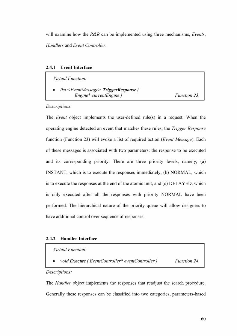
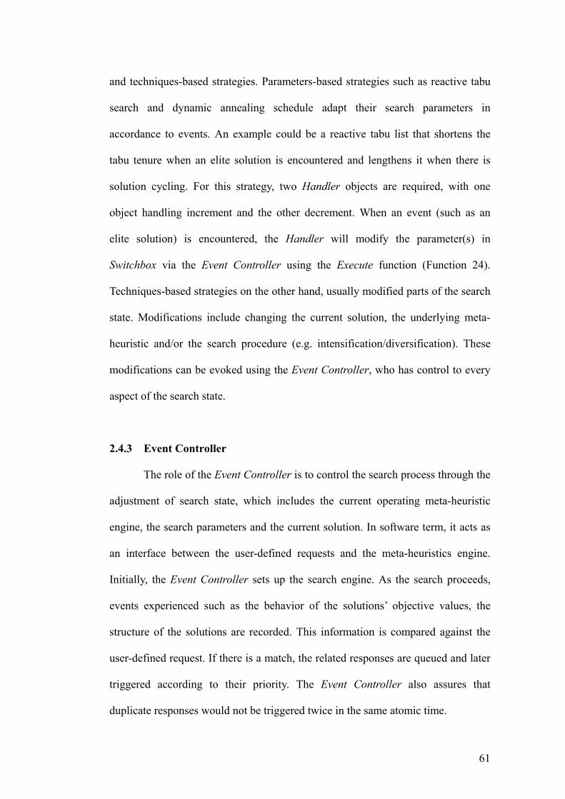
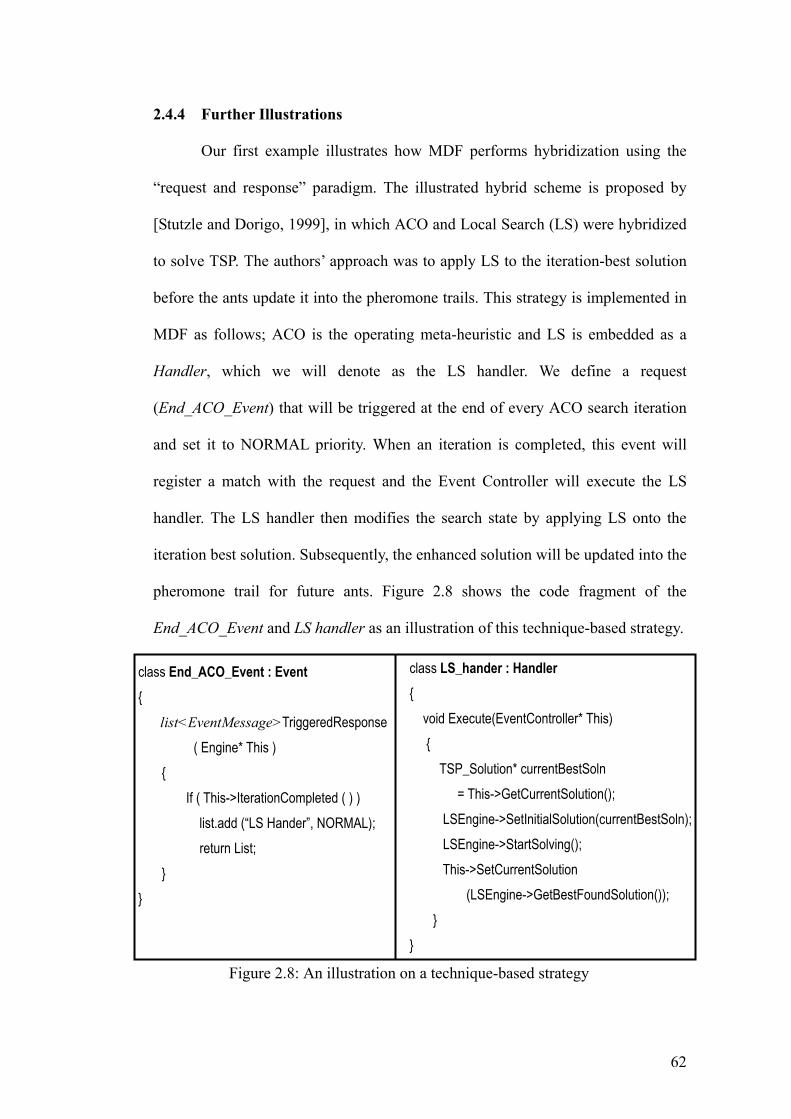
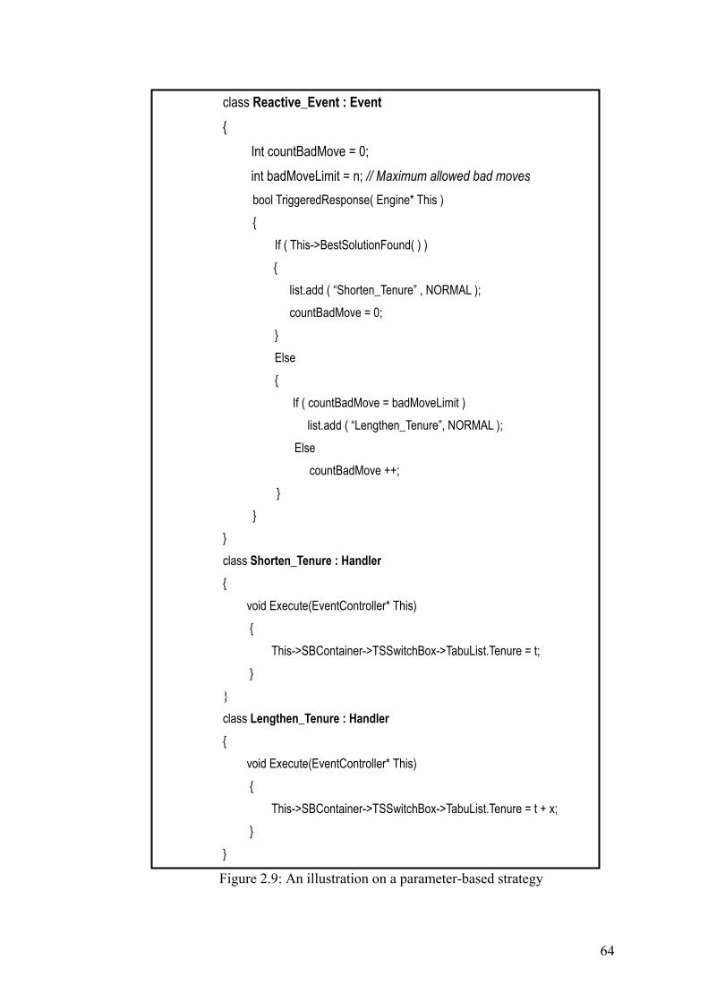
Recent computational surveys and tutorials have reported a trend whereby

meta-heuristic applications are successful in solving optimization problems, all of

which surpassed the results from traditional search methods. These promising

reports naturally captivated the attention of the research committees, especially in

the field of logistics optimization. While meta-heuristics are effective in solving

large-scale combinatorial optimization problems, in general, they result from an

extensively manual trial-and-error algorithmic design tailored to specific problems.

This leads to a diversion of resources in developing each trial algorithm, which

consequently delays the progress. Hence, the demand for a rapid prototyping tool

for fast algorithm development became a necessity. We propose Meta-Heuristics

Development Framework (MDF), a generic meta-heuristics framework that

reduces development time through abstract classes and code reuse, and more

importantly, aids design through the support of user-defined strategies and

hybridization of meta-heuristics. In this thesis, we examine two different aspects in

MDF research. First we examine the Design Concepts, which analyze the blueprint

of MDF. In this aspect, we will investigate the rationale behind the architecture of

MDF such as the interaction between the abstract classes and the meta-heuristic

engines. More interestingly, we will examine a novel way of redefining

hybridization in MDF through the “request-and-response” metaphor, which form

an abstract concept for hybridization. Different hybridization schemes can now be

formulated with relative ease, which give the proposed framework its uniqueness.

The second aspect of the thesis covers the applications of MDF, in which we take a

more “critic” role by investigating some MDF’s applications, and examining their

v

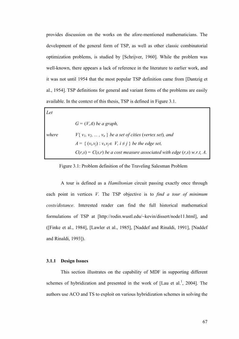
strengths and weaknesses. We begin with the Traveling Salesman Problem (TSP)

as a “walk-through” in exploring the various facets of MDF, particularly

hybridization. As TSP is a single objective, single constraint problem, the reduced

complexity makes it an ideal candidate for a comprehensive illustration. We then

extend the complexity of the TSP by increasing it into a multiple objectives,

multiple constraints problems, with potentially larger search space. The extension

results in solving the Vehicle Routing Problem with Time Windows (VRPTW), a

logistic problem that deals with finding optimal routes for serving a given number

of customers. This problem is later extended to become the Inventory and Routing

Problem with Time Windows (IRPTW), which adds inventory planning over a

defined period to the routing problem. Using the various hybridized schemes

supported by MDF, quality results can be obtained in good computational time

within relatively short developmental cycle, as presented in the experimental

results.

vi

LIST OF FIGURES 1.1 The Tabu Search (TS) Procedure 7 1.2 The pseudo code of Ants Colony Optimization (ACO) 13 1.3 The pseudo code of Simulated Annealing (SA) 18 1.4 The pseudo code of Genetic Algorithm (GA) 21 1.5 Relationships between a software library, an implementer

and a framework 27

2.1 The architecture of Meta-heuristics Development Framework 30 2.2 The relationship of Meta-heuristics behavior and MDF’s

fundamental interfaces 31

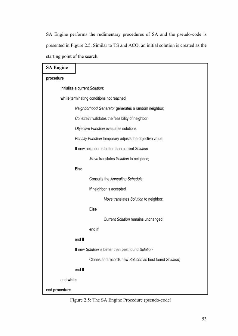
2.3 The TS Engine Procedure (pseudo-code) 48 2.4 The ACO Engine Procedure (pseudo-code) 50 2.5 The SA Engine Procedure (pseudo-code) 53 2.6 The GA Engine Procedure (pseudo-code) 55 2.7 Illustration on a feedback control mechanism 57 2.8 An illustration on a technique-based strategy 62 2.9 An illustration on a parameter-based strategy 64 3.1 Problem definition of the Traveling Salesman Problem 67 3.2 The four derived models of HASTS 69 3.3 The pseudo-code of HASTS-EA 70 3.4 Crossings and Crossing resolved by a swap operation 73 3.5 Approximation of development time 76 3.6 Result of test case KROA150 77 3.7 Result of test case LIN318 78

vii

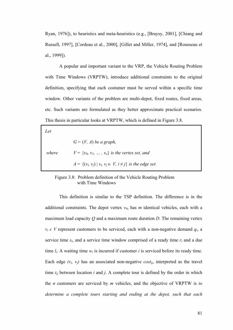
3.8 Problem definition of the Vehicle Routing Problem with Time Windows

81

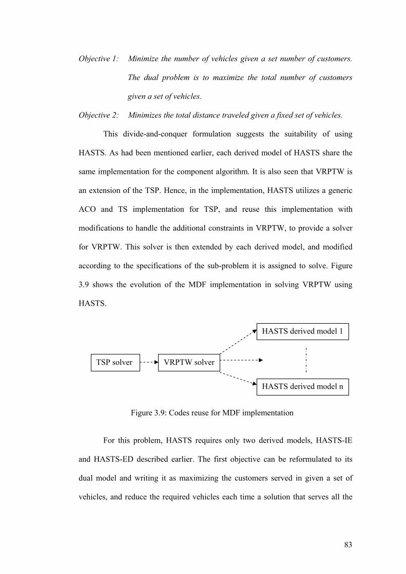
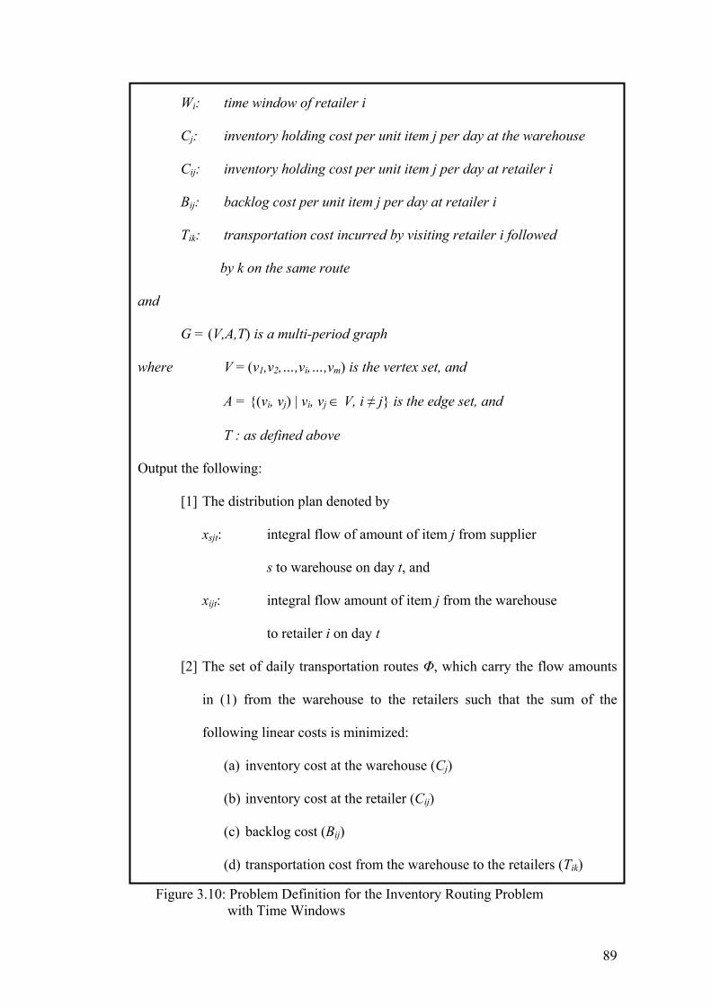
3.9 Codes reuse for MDF implementation 83 3.10 Problem Definition for the Inventory Routing Problem with

Time Windows

88

viii

LIST OF TABLES 1.1 Allegory of GA components and their evolutionary

counterparts 21

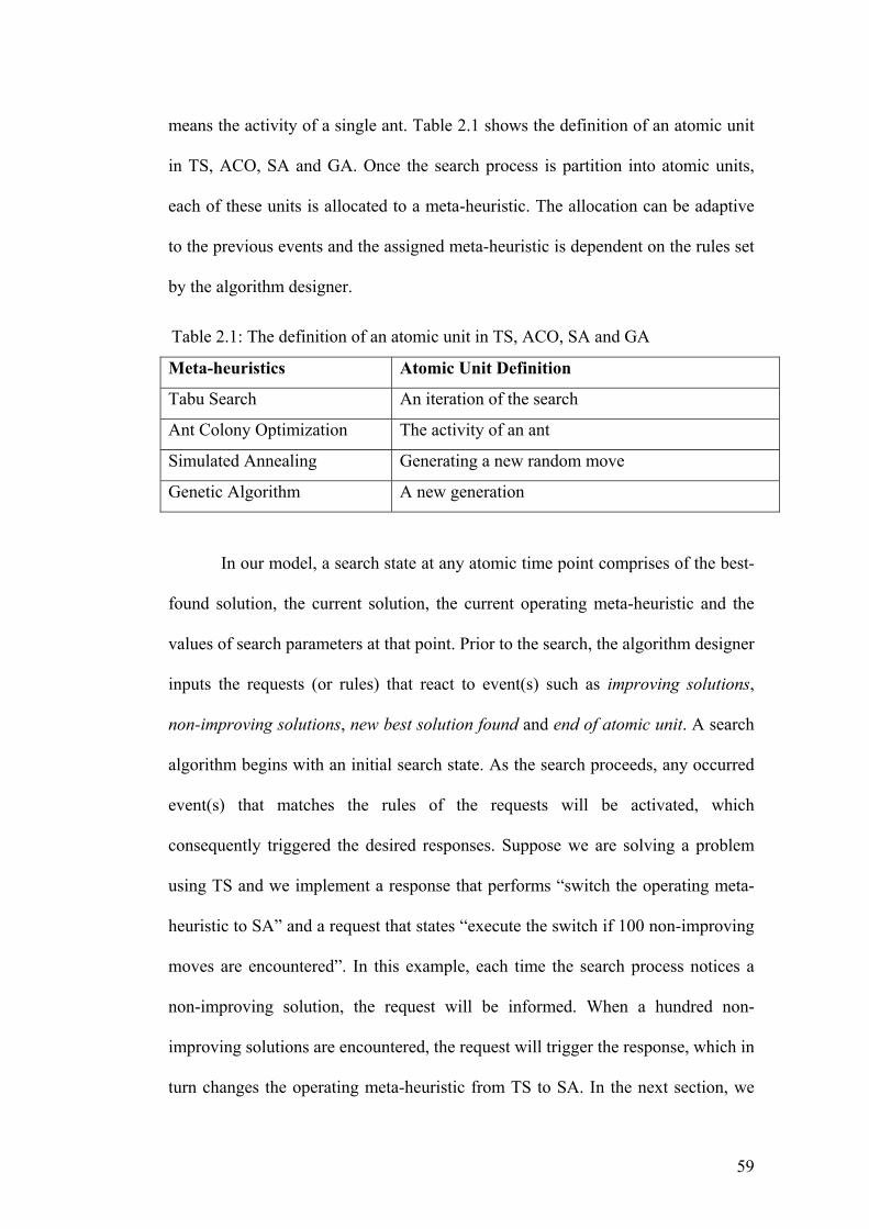
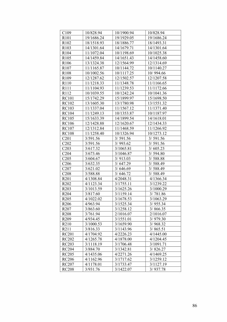
2.1 The definition of an atomic unit in TS, ACO, SA and GA 59 3.1 Results of TSP from the TSPLIB test cases 79 3.2 Results for VRPTW from the Solomon’s original test cases

(n=100) 85

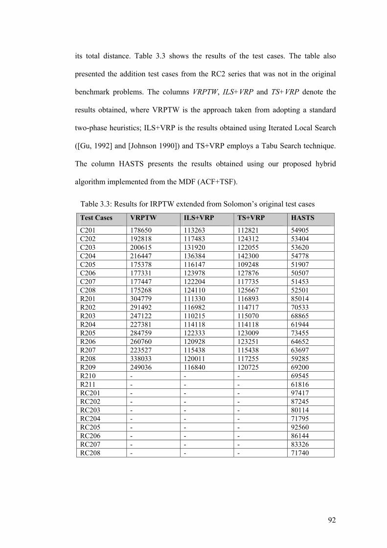
3.3 Results for IRPTW extended from Solomon’s original test

cases 92

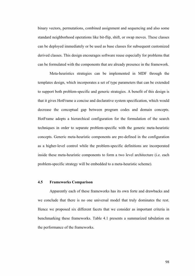
4.1 A summary of comparisons between MDF and the four

reviewed frameworks 99

ix

CHAPTER 1

INTRODUCTION

When Garey and Johnson [Garey and Johnson, 1979] revealed the

existence of non-deterministic polynomial (NP)-hard optimization problems whose

solutions are easy to verify in polynomial time, but computationally intractable to

find the optimum, it opened a new notion of NP completeness in complexity theory.

Exhaustive search is no longer a valid option as it is not only operationally

infeasible, but also impractical for finding high-quality solutions. This motivates

the development of intelligent search methods that is able to achieve good results

efficiently. Meta-heuristics matured rapidly in the recent years and becomes an

excellent replacement to exact methods, due to their effectiveness and efficiency.

On the contrary to exact methods, meta-heuristics do not guarantee the optimality

of the solution. Rather, meta-heuristics seek to obtain quality solution within a

reasonably time. As such, fast heuristics such as greedy are highly desirable as

their underlying algorithm. The basic role of meta-heuristics is then to “guide” the

heuristic from its tendency of trapping in local optimal. Each meta-heuristic has its

own unique stratagems in compensating this weakness and will be discussed in the

following sections. While the compensation may not truly offset the ineptitude, it

nevertheless yields significant improvement over the results of the greedy heuristic.

Meta-heuristic approaches has been shown to achieve promising results for

solving NP-hard problems in record time, making industry applications,

particularly in the field of logistics, very efficient. For decades, meta-heuristics

such as Tabu Search (TS), Simulated Annealing (SA), and Genetic Algorithms (GA)

have been studied in the literature for obtaining quality results from previously

1

intractable problems. Following the success of these classical meta-heuristics, there

has been an explosive growth of new techniques in line with natural and biological

observations, such as Ant Colony Optimzation (ACO) [Dorigo & Di Caro, 1999],

Squeaky Wheel [Joslin & Clements, 1999], Particle Swarm [Parsopoulos &

Vrahatis, 2002] and even mammals like lab rats [Yufik and Sheridan, 2002]. This

diffusion, while healthy for seeding new ideas into the community, is met with

such numerous and diversity that renders finding the best meta-heuristic intricate.

Till the date of this thesis, there has been no work in the literature that shows one

meta-heuristic that could truly dominate the rest for every kind of problems.

Consequently, this implies the challenge of finding the right meta-heuristic for the

right problem. The challenge is further heighten by the observation that the search

strategies used within a meta-heuristic have a considerable influence on the

effectiveness and efficiency. For example, by determining when to perform

exploitation or exploration during an ACO search can yield significant differences

in results [Dorigo & Di Caro, 1999]. As such, developers have to face the

insurmountable task of trying out different meta-heuristics with varying strategies,

and algorithmic parameters, on their problem(s).

Surprisingly, many researchers actually meet this challenge by building

meta-heuristics applications from scratch. As such, an enormous amount of

resources, in both man and machines, has to be invested for each redevelopment

that apparently is uncalled for. Ironically, the process of optimizing problems is not

optimized at all! One effective solution is to incorporate a framework that would

enable fast development through generic software design. This recycling of design

and code conserves the unnecessary wastage of resource, thus allowing researchers

to focus on the algorithmic aspects and meaningful experiments rather than

2

mundane implementation issues. However, certain criteria must be imposed to the

framework and we list three vital decisive factors.

1. It must be generic.

2. It is able to benchmark fairly on different algorithmic designs.

3. It has an unambiguous object-oriented design.

Generic has two different meanings in this context. First, the framework

must be able to work with most if not all of the combinatorial optimization

problem. Naturally, this is subjected to many criticisms as it is not viable to justify

the claim. The most convincing proof will then be providing illustration on

different applications, which in the scope of this thesis, is restricted to Routing

related problems. Secondly, generic also signifies that the framework can support

various meta-heuristics as well their strategies. This is especially important, as with

the diverse growth of meta-heuristics, we see the potential for advancing the field

further if there is provision for algorithm designers to hybridize one technique with

another. As expected, each meta-heuristic has its own forte and shortcomings and

logically leads to hybrid schemes that could exploit the strengths and cover the

weaknesses of one technique with its collaborator(s). Results from the literature

have supported the claim that such hybrid methods usually out-perform their

predecessors, e.g. [Bent & Hentenryck 2001].

The second point stresses on the role as an unbiased platform for

benchmarking, which typically refers to the comparisons of solution quality and

computational time. Although effectiveness is likely to be attributed to search

stratagems, the computational time is more often than not a controversy issue.

Aside from algorithmic efficiency, it is obvious that the technical skill of an

implementer has a considerable impact on the overall competency. A framework

3

should therefore provide a developmental platform that neglects the impact of

programming proficiency. This achieves a more precise comparison on the

algorithms’ efficiency. Bearing this in mind, the framework should reduce the

development efforts to minimal by off-loading the routine of meta-heuristics, as

well as incorporating a software library for rapid development. Finally, the last

point states a software engineering requirement, which may not seem essential but

is highly sought-after. Object-Oriented Programming (OOP) is adopted because of

its clarity in design and ease of integration and extension. As the framework is

likely to be a complex tool, each abstract class should be unambiguous and clearly

defined for its role. Advantages of a well-designed architecture could give

implementers fewer frustrating development hours and is also less prone to

programming errors.

By now it is apparent that there is a powerful motivation for a meta-

heuristics framework. We propose the Meta-heuristics Development Framework

(MDF) as an aspirant to compete with other works in the literature. Powered by

four different meta-heuristics, MDF provides a platform for both rapid prototyping

as well as unbiased benchmarking. The potency of MDF lies in its unique control

mechanism, which allows hybridization to be formed effortlessly. In addition, the

control mechanism follows the “request-and-response” analogy, which enhances

comprehension and easily adopted. The framework also bridges the algorithm

designers and the program implementers by having no constraint on the

formulation of strategies, thus giving liberty to the designers’ imagination and yet

easily accommodated by the implementers. In short, MDF is a generic, flexible

framework that is constrained only by the developers’ mind rather than the

restrictions in framework.

4

The following two sections in this chapter will give a short account on the

meta-heuristics’ background and some software engineering concepts. For readers

who are more concerned with MDF issues, these sections can be skipped without

affecting the rest of the thesis. Chapter 2 will be examining the design concepts of

MDF, which we termed as fundamental research and development. In this chapter,

we will be exploring the conceptual design and appreciate the rationale leading to

its architecture. Illustrations and pseudo-codes can be found throughout the chapter

to enhance its comprehension. Chapter 3 focuses on the applications of MDF,

particularly to illustrate the flexible design and reuse capability. The chapter will

start off with Traveling Salesman Problem (TSP), whose simplicity makes it an

excellent illustration on the various formulations of hybridization scheme. It is then

demonstrated how instance implementations for the Vehicle Routing Problem with

Time Windows (VRPTW), using TSP implementations, are solved, and further

extended to solve the Inventory Routing Problem with Time Windows (IRPTW)

with promising results. Results from solving these problems (TSP, VRPTW and

IRPTW) are also presented to prove the case. Through these applications, it is

demonstrated how the framework allowed reuse and recycle, which reduces

development time and yet provides excellent results. The experimental results have

shown the effectiveness of the proposed framework. Competitors of MDF in the

literature are reviewed in Chapter four, which gives an account on their pros and

cons. Finally, Chapter five concludes the thesis by reporting the current

development and proposing some future extension that is insightful for the growth

of MDF.

1.1 Meta-heuristics Background

5

Meta-heuristics are as flexible as the ingenuity of the algorithm designer,

and they can be inspired from physics, biology, nature and any other fields of

science. This section provides some backgrounds on the four meta-heuristics that

are incorporated in MDF and they are Tabu Search (TS), Ant Colony Optimization

(ACO), Simulated Annealing (SA) and Genetic Algorithm (GA). Important concepts

are introduced to enhance the readers’ comprehension on the stratagems discussed

in the later chapters of this thesis.

1.1.1 Tabu Search (TS)

History

The roots of TS can be traced back to the 1970's and was first formally introduced

in its present form by [Glover, 1986]. Incidentally, the basic ideas had also been

sketched in the works of [Hansen, 1986]. Additional efforts of formalization are

later reported in [Glover, 1989], [de Werra & Hertz, 1989], [Glover, 1990]. Many

computational experiments have shown TS to be competitive against most known

techniques and through its flexibility, could out-perform many classical

procedures. Surprisingly till today, there is yet a formal explanation of this good

behavior. Theoretical aspects of TS have been investigated in the works of ([Faigle

& Kern, 1992], [Fox, 1993]). A didactic presentation of tabu search and a series of

applications have also been collected in a book [Glover, Taillard, Laguna & de

Werra, 1993]. Its interest lies in the fact that success with tabu search often implies

that a serious effort of modeling was done from the beginning. The applications in

[Glover and Laguna, 1997] provide many such examples together with a collection

of references.

6

Basic Concept

Formally let us consider an optimization problem in the following way: Given a set

S of feasible solutions and a function f : S → ℜ, find some solution i* in S such

that f(i*) is acceptable subjected to some constraints. Generally the acceptability

for a solution i* is to have f(i*) ≤ f(i) for every i in S. In such a situation TS would

be an exact minimization algorithm provided the exploration process can guarantee

that after a finite number of steps such an i* would be reached. However in most

situation, there is no guarantee on an i* and therefore TS could simply be viewed

as an extremely general heuristic procedure. The general procedure of TS is

presented in Figure 1.1.

Tabu Search

Step 1. Choose an initial solution i in S. Set i* = i and k = 0.

Step 2. Set k = k+1 and generate a subset V* of solution in N(i,k) such

that either one of the tabu conditions is violated or at least one

of the aspiration conditions holds.

Step 3. Choose a best j = i Å m in V* (with respect to f )

and set i = j.

Step 4. If f(i) < f(i*) then set i* = i.

Step 5. Update tabu and aspiration conditions.

Step 6. If a stopping condition is met, then stop. Else go to Step 2.

s

Figure 1.1: The Tabu Search (TS) Procedure

Generally V* = N(i), which indicates the complete neighbor

the current solution i. However this neighborhood is often lar

time-consuming to search each individual. Hence an appropri

be a substantial improvement. The iterative exploration pr

Notation

S: Available Search Space i: Current Solution i*: Best Found Solution k: Current iteration N(i,k): Neighborhood

hood generated from

ge and it may be too

ate size of V* would

ocess (local search)

7

should accept non-improving moves from i to j in V* (i.e. f(j) > f(i)) if one would

like to escape from a local minimum. However, as soon as non-improving moves

are possible, the risk of re-visiting a solution (cycling) becomes a serious concern.

TS reduces this likelihood through the use of memory, which forbids moves that

might lead to recently visited solutions. If such a memory is introduced, the

structure of N(i) will depend upon the iteration k and so the neighborhood becomes

N(i,k) instead of N(i). It is important to realize that the definition of N(i, k) at each

iteration k and the choice of V* are crucial. The definition of N(i, k) implies that

some recently visited solutions are removed from N(i). These removed solutions

are known as “tabu-ed” solutions and should be avoided in some future iterations.

Such usage of recency-based memory will prevent cycling for the length of “tabu-

ed” duration (tabu tenure). For instance, keeping at iteration k a tabu list of the last

T solutions visited will prevent cycles of size at most T. However, keeping a tabu

list of the last T solutions is sometimes cumbersome and it is often simplified to

keep track of the last T moves associated with the translation of i to j (j = i ⊕ m). It

is clear that this restriction has a loss of information and hence will have no

guarantee that there is no cycling for a length of T. The drawback of the

simplification (replacement of solutions by moves) could result in giving a “tabu-

ed” status to solutions which may be unvisited so far. As such, it is compelled to

have a relaxation on the tabu status when the tabu-ed solutions will look attractive.

This relaxation is known as aspiration criterion. For example, a tabu-ed move m

applied to a current solution i may appear attractive because it results in a solution

that is better than the best found so far. Finally the stopping conditions also assert

certain influence on the search procedure and some immediate stopping conditions

could be the following:

8

• N(i, k+1) = NULL

• k is larger than the maximum number of iterations allowed

• The number of iterations since the last improvement of i* is larger than a

specified number

• Evidence can be given than an optimum solution has been obtained.

Stratagems

Most of the TS stratagems are associated the memory. So far the described usage

of memory is an essential part of TS and is considered as a short term memory that

prevents cycling to some extent. On the other hand, long term memory often

involves collecting information from the search and applied strategies in response

to these information. Among these strategies, there are three distinctive tactics,

variable (reactive) tabu list size, intensification and diversification.

Reactive tabu list

The basic role of the tabu list is to prevent cycling. Ideally, the tabu tenure should

be small as a lengthy list affects both the search efficiency as well as the memory

consumption. However, if the length of the list is too small, the role might not be

achieved. Given an optimization problem it is often difficult or even impossible to

determine a value that prevents cycling and does not excessively restrict the search

for all instances of the problem of a given problem size. An effective way for

circumventing this difficulty is to use a tabu list with variable size. The size of the

list would response to the search information based on the instance it is solving and

changes accordingly. To prevent extreme sizes being used, it is often bounded by

given maximal and minimal values.

9

Intensification

Intensifying strategies are based on the assumption that better solutions can be

found by exploring the search space around elite solutions. In order to intensify the

search in promising regions, a preliminary search is performed to collect a list of

elite solutions (mostly local optimal). Each elite solution is then “examined”

closely by decreasing the size of the tabu list for a small number of iterations. In

some cases, more elaborate techniques may be used. Another strategy inspired

from the classic divide-and-conquer paradigm consists of partitioning an

optimization problem into sub-problems, solving them (optimally) and finally

combining the partial solutions. A post-optimization phase may sometimes be

performed on the combined solution. Obviously, the difficulty lies in finding a

good partitioning technique. Other ways for intensifying the search are the use of

more elaborate heuristics or even exact methods, or the enlargement of the

neighborhood around elite solutions. It is also possible to perform an

intensification based on long term memory. As each solution or move can be

characterized by certain components for their "goodness", these components are

memorized for future selection of neighbors. This usage of long term memory can

be viewed as a kind of learning process.

Diversification

As oppose to intensification, diversifying strategies focus on searching the

unexplored regions. While intensification attempts to improve on the solution

quality, it is not necessary for a solution to diversify to a better neighbor. The

underlying notion is to “jump” away from the current solution structure. The

simplest diversification is to perform random restarts. A different approach which

10

ensures the exploration of unvisited regions is to penalize frequently performed

moves or certain component(s) presence in the neighbors. Some diversifications

involve oscillating between feasible and infeasible solutions. This is achieved by

relaxing the constraints for a small number of iteration before repairing the

feasibility. However, there are times in which the solution is beyond repair and it is

then necessary to “backtrack” to the original solution or to restart the search again.

1.1.2 Ants Colony Optimization (ACO)

History

Ant Colony Optimization (ACO) is a recently proposed meta-heuristic approach,

which is inspired from the foraging behavior of real ants using pheromones as a

communication medium. In analogy to the biological example, ACO is based on

the indirect communication of a colony of simple agents, called (artificial) ants,

mediated by (artificial) pheromone trails. The pheromone trails in ACO serve as

distributed, numerical information, in which individual ants use to probabilistically

construct solutions. The ants adapt by “depositing” different amount of pheromone

to reflect their search experience. The first ACO algorithm proposed was Ant

System (AS) [Dorigo et al., 1991]. At the early stage, AS was applied to some

rather small instances of the TSP with the problem size of up to 75 cities.

Experimental results show that it was more than a match in performance compared

to other meta-heuristics such as evolutionary computation ([Dorigo, 1992], [Dorigo

et al., 1996]). Despite the initial encouraging results, AS loses its edges for large

instances in TSP. Since then, a substantial amount of research has been invested on

ACO algorithms. The more recent algorithms are direct extensions of AS with

added advanced features, and have established their creditability in obtaining good

11

results ([Dorigo and Gambardella, 1997], [Dorigo and Di Caro, 1999]). Ironically,

while these features improve on the effectiveness, they also render the behaviors of

ACO to draft away from the resemblance of its biological counter-parts.

Basic Concept

While TS is considered as an enhancement to the local search technique, ACO can

be interpreted as an extension of traditional construction heuristics. Informally, the

ACO algorithm can be summarized as follows: A colony of ants is concurrently

and asynchronously moving through adjacent states of the problem, which

incrementally build up a solution to the optimization problem. Each “chosen” state

depends on a stochastic local decision policy that uses a combination of

pheromone trails and heuristic information. During the construction of a solution,

the ant evaluates the (partial) solution and deposits pheromone trails on the

components or connections it used. This pheromone information is used later to

direct the search of the future ants. Beside the ants’ activity, there are two other

concurrent events, pheromone trail evaporation and daemon actions. Pheromone

evaporation is the process in which the pheromone trail intensity on the

components decreases over time. This phenomenon is necessary to avoid a rapid

convergence towards a sub-optimal region. Analogically, it can be seen as

“forgetting” the previously favored paths and begins the exploration of new areas

of the search space. Daemon actions are used to implement centralized actions

which cannot be performed by a single ant. For example, a daemon action can be

the collection of global information that can be used to decide whether it is useful

to deposit additional pheromone to guide the search process away from local

optimum. A pseudo code of ACO is presented in Figure 1.2.

12

Ants Colony Optimization

procedure ACO

ScheduleActivities

ManageAntsActivity()

EvaporatePheromone()

DaemonActions()

end ScheduleActivities

end ACO

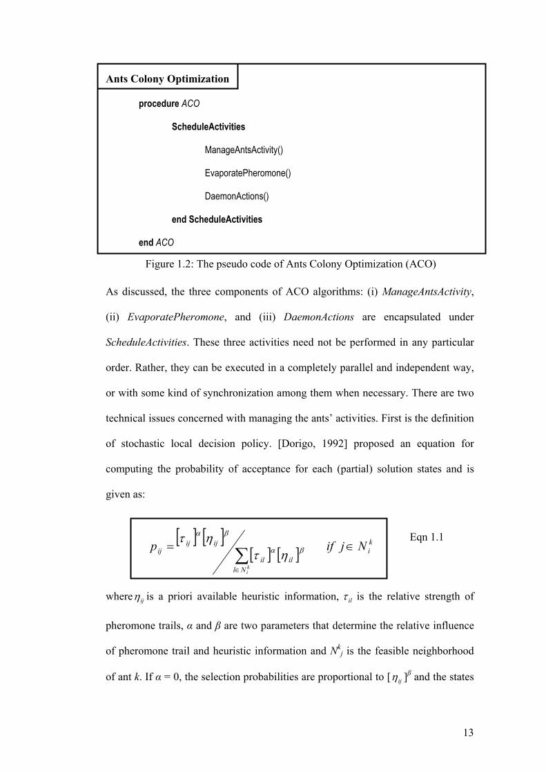
Figure 1.2: The pseudo code of Ants Colony Optimization (ACO)

As discussed, the three components of ACO algorithms: (i) ManageAntsActivity,

(ii) EvaporatePheromone, and (iii) DaemonActions are encapsulated under

ScheduleActivities. These three activities need not be performed in any particular

order. Rather, they can be executed in a completely parallel and independent way,

or with some kind of synchronization among them when necessary. There are two

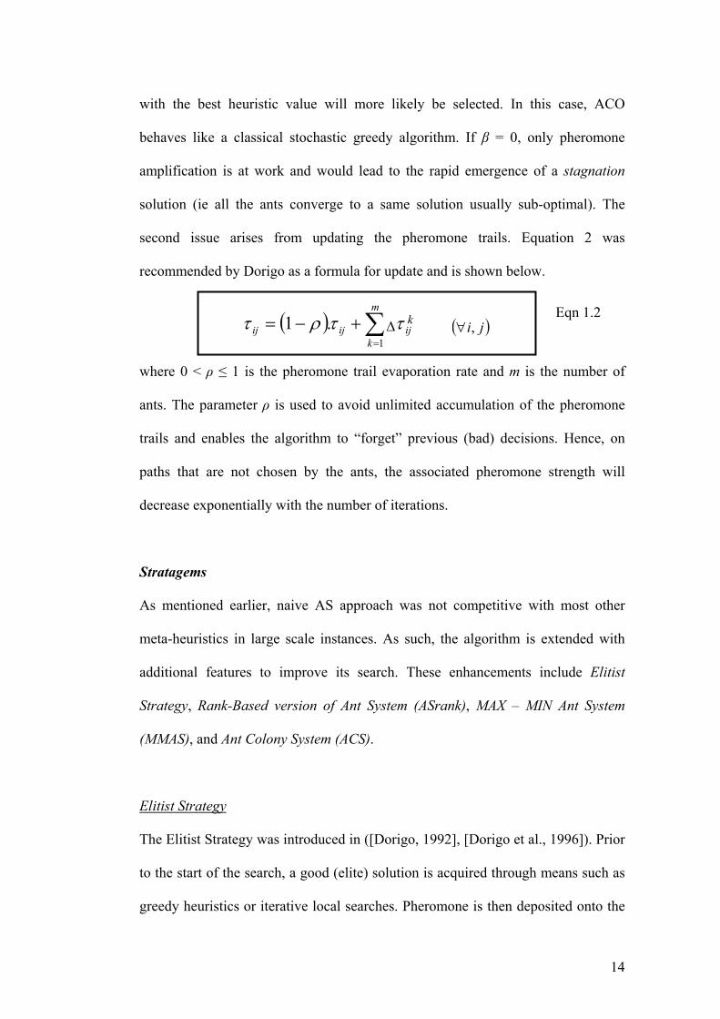
technical issues concerned with managing the ants’ activities. First is the definition

of stochastic local decision policy. [Dorigo, 1992] proposed an equation for

computing the probability of acceptance for each (partial) solution states and is

given as:

[ ] [ ][ ] [ ]

ki

Nlilil

ijijij Njifp

ki

∈=∑∈

βα

βα

ητητ Eqn 1.1

where ijη is a priori available heuristic information, ilτ is the relative strength of

pheromone trails, α and β are two parameters that determine the relative influence

of pheromone trail and heuristic information and Nkj is the feasible neighborhood

of ant k. If α = 0, the selection probabilities are proportional to [ ijη ]β and the states

13

with the best heuristic value will more likely be selected. In this case, ACO

behaves like a classical stochastic greedy algorithm. If β = 0, only pheromone

amplification is at work and would lead to the rapid emergence of a stagnation

solution (ie all the ants converge to a same solution usually sub-optimal). The

second issue arises from updating the pheromone trails. Equation 2 was

recommended by Dorigo as a formula for update and is shown below.

( )ji,∀( ) ∑=

+−=m

kijijij

1

.1 τρτ τ∆ k Eqn 1.2

where 0 < ρ ≤ 1 is the pheromone trail evaporation rate and m is the number of

ants. The parameter ρ is used to avoid unlimited accumulation of the pheromone

trails and enables the algorithm to “forget” previous (bad) decisions. Hence, on

paths that are not chosen by the ants, the associated pheromone strength will

decrease exponentially with the number of iterations.

Stratagems

As mentioned earlier, naive AS approach was not competitive with most other

meta-heuristics in large scale instances. As such, the algorithm is extended with

additional features to improve its search. These enhancements include Elitist

Strategy, Rank-Based version of Ant System (ASrank), MAX – MIN Ant System

(MMAS), and Ant Colony System (ACS).

Elitist Strategy

The Elitist Strategy was introduced in ([Dorigo, 1992], [Dorigo et al., 1996]). Prior

to the start of the search, a good (elite) solution is acquired through means such as

greedy heuristics or iterative local searches. Pheromone is then deposited onto the

14

“path” contained in the elite solution. When the search begins, the additional

pheromone will render the ants to favor taking the “good” paths. Hence, this

strategy can be also viewed as intensifying the ants to search around the elite

solution.

Rank-Based Ants System (ASrank)

Following the same concept of intensification, ASrank [Bullnheimer et. al., 1999]

can be seen as an extension of the Elitist Strategy. For each round of optimization

(iteration), the solutions constructed by the ants are sorted according to their

quality. The best w solution is then selected to be updated into the pheromone

trails. In addition, the strength of the updated pheromone depends on the quality of

the solution. For example, the r best ant will be updated with (w – r) amount of

pheromone onto its trail. An advantage of this strategy is that it removes the false

trails left by poorly constructed solutions, and hence reduces the probability of

constructing poor solutions.

MAX –MIN Ant System (MMAS)

In MMAS ([Stutzle et al., 1997], [Stutzle, 1999], [Stutzle et al., 2000]), upper and

lower bounds are enforced to the values of the pheromone trails, as well as a

different initialization of their values. This helps to avoid sudden convergence to

stagnation solution and promote a higher degree of exploration. For each round of

optimization, MMAS only update the best ants’ trail (the global-best or the

iteration-best ant). Similar to the ASrank, the idea is to prevent deposition of

pheromone in false trails. Computational results have shown that best results are

15

obtained when pheromone updates are performed using the global-best solution

with increasing frequency during the algorithm execution.

Ants Colony System (ACS)

ACS ([Gambardella and Dorigo, 1996], [Dorigo and Gambardella, 1997]) focuses

more on the exploitation of information collected by previous ants than the

exploration of the search space. There are three mechanisms involved. Firstly, a

pseudo-random proportional rule [Dorigo and Gambardella, 1997] is used to guide

the ants in choosing their “paths”. This rule uses a parameter q0 to determine

whether an ant is performing exploitation or exploration. In exploitation, the ants

are stimulated to intensify their search on paths with stronger pheromone whereas

in exploration, the ants are encouraged to diversify their search on unexplored

ground. When the value q0 is set to a value close to 1, the ants will favor

exploitation over exploration. Conversely, when q0 is set to 0, the probabilistic

decision rule becomes the same as in AS. Secondly, ACS follows the concepts of

MMAS by only updating the trails of the best ants with pheromone. The best ants

could be the global-best or the iteration-best ants. Thirdly, to counter the effect of

over-exploitation, the last mechanism (known as the local evaporation), is used to

lessen the pheromone on a trail whenever an ant moves through it. The local

evaporation can be imagined as ants “absorbing” some of the pheromone as they

move along the trails. The effect is to encourage subsequent ants to explore new

regions rather than to follow previous ants’ paths. In addition to the three

mechanisms, some ACS algorithms also incorporate local search to enhancement

their results.

16

1.1.3 Simulated Annealing (SA)

History

In 1983 three IBM researchers [Kirkpatrick et al., 1983] published a paper in

Science magazine called Optimization by Simulated Annealing. The authors

described a computational intensive algorithm for finding solutions to general

optimization problems. Their method is based on the way nature performs an

“optimization of energy” of a crystalline solid when it is annealed to remove

defects in the atomic arrangement. As an analogy to this physical process,

Simulated Annealing (SA) uses the objective function of an optimization problem

instead of the energy level of a real material. The simulated thermal fluctuations

are changes in the adjustable parameters of the problem rather than atomic

positions. If the annealing schedule achieves effective thermal equilibrium at each

temperature (i.e., enough accepted random moves), then the objective function

reaches its global minimum when the simulated temperature reaches the vicinity of

zero.

Basic Concept

SA is a global optimization method that distinguishes between different local

optimal. Starting from an initial point, the algorithm generates a random neighbor

and the objective function is evaluated on the neighbor. Any improving move is

accepted and the process repeats from this new point. However, a non-improving

move may be accepted in order to allow the search to escape from local optimal.

This “anti-greedy” decision is made by the Metropolis criteria [Metropolis et al.

1953]. Generally, as the optimization process proceeds, the probability of

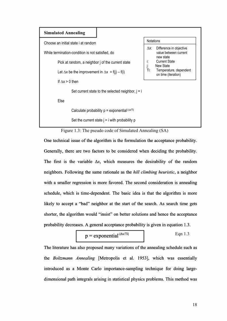
acceptance declines. The complete pseudo code is presented in Figure 1.3.

17

Simulated Annealing

Choose an initial state i at random

While termination-condition is not satisfied, do

Pick at random, a neighbor j of the current state

Let ∆x be the improvement in ∆x = f(j) – f(i)

If ∆x > 0 then

Set current state to the selected neighbor, j = i

Else

Calculate probability p = exponential-|∆x/Ti|

Set the current state j = i with probability p

s

Figure 1.3: The pseudo code of Simulated An

One technical issue of the algorithm is the formulation

Generally, there are two factors to be considered wh

The first is the variable ∆x, which measures the

neighbors. Following the same rationale as the hill cli

with a smaller regression is more favored. The secon

schedule, which is time-dependent. The basic idea is

likely to accept a “bad” neighbor at the start of the

shorter, the algorithm would “insist” on better solution

probability decreases. A general acceptance probability

One technical issue of the algorithm is the formulation

Generally, there are two factors to be considered wh

The first is the variable ∆x, which measures the

neighbors. Following the same rationale as the hill cli

with a smaller regression is more favored. The secon

schedule, which is time-dependent. The basic idea is

likely to accept a “bad” neighbor at the start of the

shorter, the algorithm would “insist” on better solution

probability decreases. A general acceptance probability

p = exponential-|∆x/Ti|

The literature has also proposed many variations of the

the Boltzmann Annealing [Metropolis et al. 195

introduced as a Monte Carlo importance-sampling

dimensional path integrals arising in statistical physics

The literature has also proposed many variations of the

the Boltzmann Annealing [Metropolis et al. 195

introduced as a Monte Carlo importance-sampling

dimensional path integrals arising in statistical physics

p = exponential-|∆x/Ti|

Notation

∆x: Difference in objective value between current new state i: Current State j: New State Ti: Temperature, dependent on time (iteration)

nealing (SA)

the acceptance probability.

en deciding the probability.

desirability of the random

mbing heuristic, a neighbor

d consideration is annealing

that the algorithm is more

search. As search time gets

s and hence the acceptance

is given in equation 1.3.

the acceptance probability.

en deciding the probability.

desirability of the random

mbing heuristic, a neighbor

d consideration is annealing

that the algorithm is more

search. As search time gets

s and hence the acceptance

is given in equation 1.3.

annealing schedule such as

3], which was essentially

technique for doing large-

problems. This method was

annealing schedule such as

3], which was essentially

technique for doing large-

problems. This method was

Eqn 1.3

18

later generalized to apply on non-convex cost-functions arising from a variety of

optimization problems. Fast Annealing [Szu and Hartley, 1987] was later extended

from the Boltzmann Annealing, by replacing the Boltzmann forms with the

Cauchy distribution.

Stratagems

In most optimization, SA is rarely used alone. This is because of the lengthy

computational time involved before the algorithm could obtain quality results. On

the other hand, SA excellent capability in escaping from local optimal made it too

valuable to be ignored. As such, modern techniques often hybridize SA (or its

variations) as a mechanism to escape local entrapment. For example, a simple

hybrid scheme can be formed with the hill-climbing heuristic. The hill-climbing

heuristic is an iterative improvement technique that adopted a greedy approach to

increase the solution quality. When the heuristic is ensnared in local optimal, SA

could then be applied as a “kick” to diversify the search to a new region. In such

stratagem, SA acts as a probabilistic diversifier and has been known to obtain good

results when hybridize in similar fashion with many other meta-heuristics.

1.1.4 Genetic Algorithm (GA)

History

GA originated from the studies of cellular automata, conducted by Holland

[Holland, 1992], and his colleagues at the University of Michigan. Holland’s book

that was published in 1975 is generally acknowledged as the beginning of the

research of GA. Until the early 1980s, the research in genetic algorithms was

mainly theoretical [Davidor, 1991], with few real applications. From the early

19

1980s the community of genetic algorithms has experienced an abundance of

applications which spread across a large range of disciplines. Each and every

additional application gave a new perspective to the theory. Furthermore, in the

process of improving performance, new and important findings regarding the

generality, robustness and applicability of genetic algorithms became available.

Following the last decades of rapid development, GA, in various guises has been

successfully applied to various optimization problems.

Basic Concept

Genetic algorithm is a model of machine learning that derives its behavior from a

metaphor of the processes of evolution in nature. A population of individuals can

be represented by their chromosomes. Nature compels each individual to go

through a process of evolution which, according to [Darwin, 1979], is made up of

the principles of selection and mutation. The selection process allows only the

“fittest” to survive and consequently passed down their genes to their offspring.

Natural mutation on the other hand, “alters” the individuals’ chromosomes, usually

to improve survivability. Allegory, an optimization can be formulated as an

evolutionary process. For example, a solution can be represented as a set of

characters or byte/bit strings, which corresponds to the chromosomes. The

selection criterion then becomes the objective function. Table 1.1 gives a list of

GA components with its evolutionary counterparts. With these components in

place, the pseudo-code of GA is presented in Figure 1.4.

20

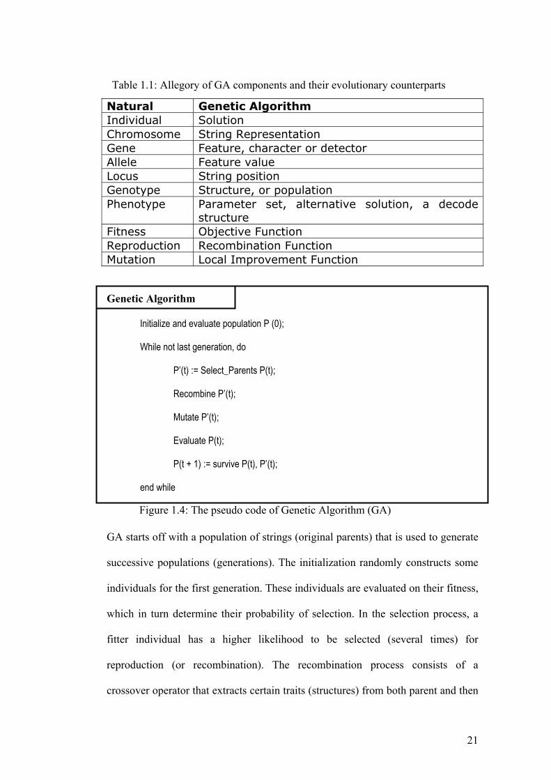
Table 1.1: Allegory of GA components and their evolutionary counterparts

Natural Genetic Algorithm Individual Solution Chromosome String Representation Gene Feature, character or detector Allele Feature value Locus String position Genotype Structure, or population Phenotype Parameter set, alternative solution, a decode

structure Fitness Objective Function Reproduction Recombination Function Mutation Local Improvement Function

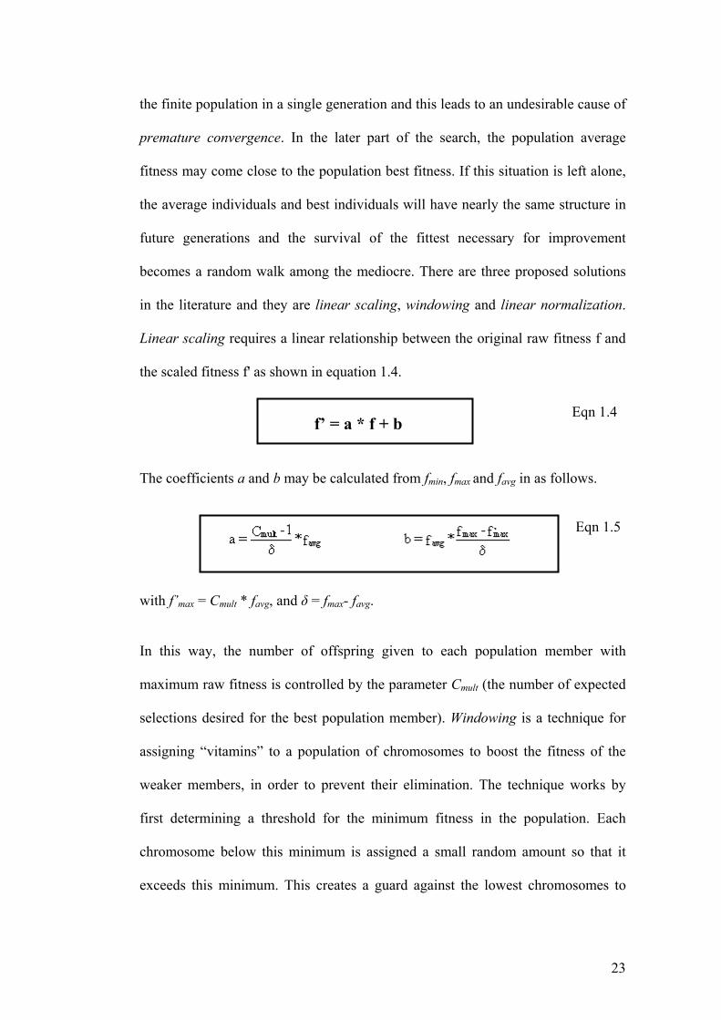
Genetic Algorithm

Initialize and evaluate population P (0);

While not last generation, do

P’(t) := Select_Parents P(t);

Recombine P’(t);

Mutate P’(t);

Evaluate P(t);

P(t + 1) := survive P(t), P’(t);

end while

Figure 1.4: The pseudo code of Genetic Algorithm (GA)

GA starts off with a population of strings (original parents) that is used to generate

successive populations (generations). The initialization randomly constructs some

individuals for the first generation. These individuals are evaluated on their fitness,

which in turn determine their probability of selection. In the selection process, a

fitter individual has a higher likelihood to be selected (several times) for

reproduction (or recombination). The recombination process consists of a

crossover operator that extracts certain traits (structures) from both parent and then

21

recombines them to form a new offspring. Each offspring then undergoes a

mutation process, in which some fast heuristics are used to improve on its fitness.

Sometimes, these new offspring are evaluated and mixed with their parents. Finally

a new generation is obtained through sampling of the combined population to

remove away the individuals who are considered as “unfit”. The algorithm is then

repeated for a pre-determined number of generations. It is essential for the solution

to be formulated as characters or byte strings before GA can be applied. This

restriction demands some ingenuity from the algorithm designers when they devise

their approaches. In addition, the modeling of GA does not take into account the

possibility of infeasible solutions. In GA, infeasible solutions are often treated as

“unfit” individual and eventually discarded. However, there is no mechanism that

prevents producing infeasible individual and thus renders the algorithm to be less

suitable for problems with tight constraints.

Stratagem

Aside from hybridization (which will be discussed further in Chapter 2), there are

several strategies that improve the effectiveness and efficiency of GA search.

Usually these strategies involve one or more GA components collaborating

together. Among these strategies, we introduce Fitness Techniques, Elitism, Linear

Probability Curve and Steady Rate Reproduction.

Fitness Techniques

At the start of GA search, it is common to have a few elite individuals in a

population of mediocre contemporaries. If left to the normal selection rule of the

simple GA, the elite individuals would soon take over a significant proportion of

22

the finite population in a single generation and this leads to an undesirable cause of

premature convergence. In the later part of the search, the population average

fitness may come close to the population best fitness. If this situation is left alone,

the average individuals and best individuals will have nearly the same structure in

future generations and the survival of the fittest necessary for improvement

becomes a random walk among the mediocre. There are three proposed solutions

in the literature and they are linear scaling, windowing and linear normalization.

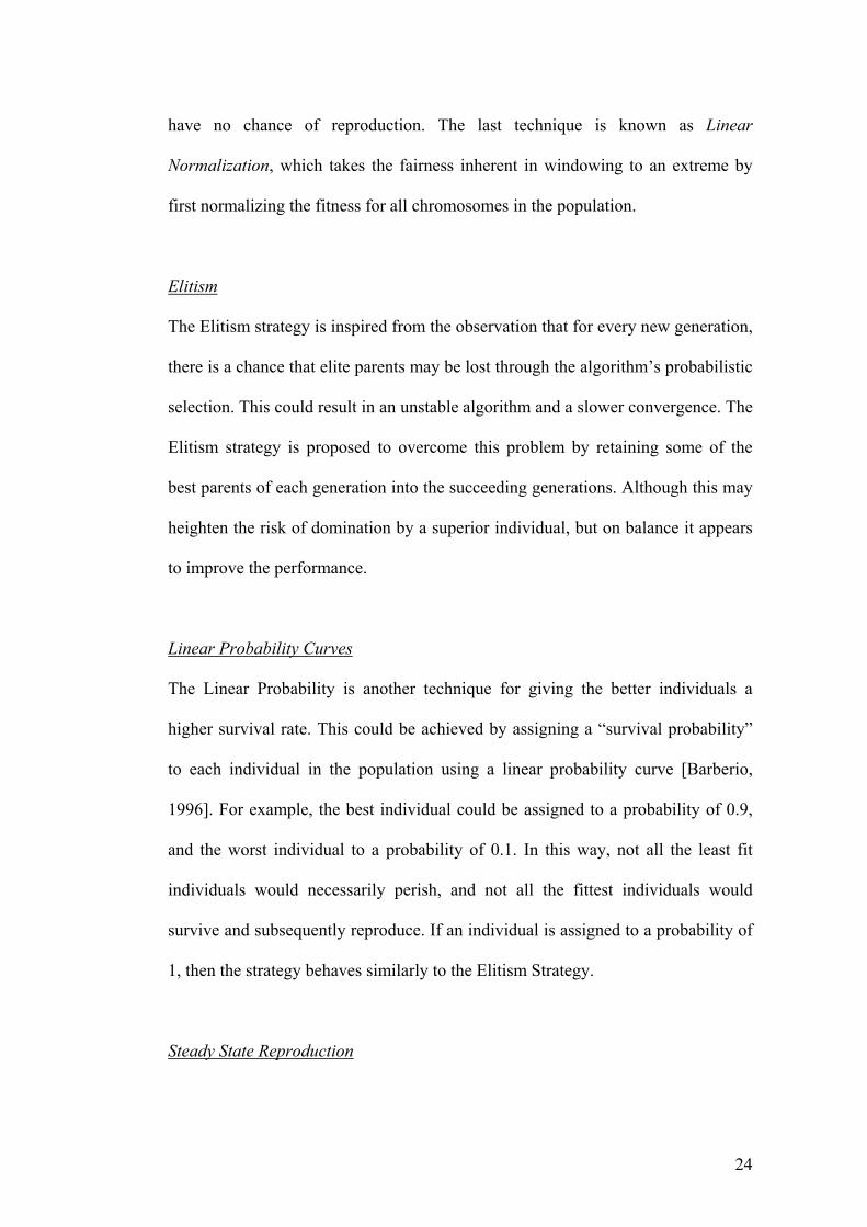
Linear scaling requires a linear relationship between the original raw fitness f and

the scaled fitness f' as shown in equation 1.4.

f’ = a * f + b Eqn 1.4

The coefficients a and b may be calculated from fmin, fmax and favg in as follows.

Eqn 1.5

with f’max = Cmult * favg, and δ = fmax- favg.

In this way, the number of offspring given to each population member with

maximum raw fitness is controlled by the parameter Cmult (the number of expected

selections desired for the best population member). Windowing is a technique for

assigning “vitamins” to a population of chromosomes to boost the fitness of the

weaker members, in order to prevent their elimination. The technique works by

first determining a threshold for the minimum fitness in the population. Each

chromosome below this minimum is assigned a small random amount so that it

exceeds this minimum. This creates a guard against the lowest chromosomes to

23

have no chance of reproduction. The last technique is known as Linear

Normalization, which takes the fairness inherent in windowing to an extreme by

first normalizing the fitness for all chromosomes in the population.

Elitism

The Elitism strategy is inspired from the observation that for every new generation,

there is a chance that elite parents may be lost through the algorithm’s probabilistic

selection. This could result in an unstable algorithm and a slower convergence. The

Elitism strategy is proposed to overcome this problem by retaining some of the

best parents of each generation into the succeeding generations. Although this may

heighten the risk of domination by a superior individual, but on balance it appears

to improve the performance.

Linear Probability Curves

The Linear Probability is another technique for giving the better individuals a

higher survival rate. This could be achieved by assigning a “survival probability”

to each individual in the population using a linear probability curve [Barberio,

1996]. For example, the best individual could be assigned to a probability of 0.9,

and the worst individual to a probability of 0.1. In this way, not all the least fit

individuals would necessarily perish, and not all the fittest individuals would

survive and subsequently reproduce. If an individual is assigned to a probability of

1, then the strategy behaves similarly to the Elitism Strategy.

Steady State Reproduction

24

When the simple GA reproduces, it replaces its entire set of parents by their

children. This technique has some potential drawbacks and even with an Elitism

Strategy, there is no guarantee that the best individuals would reproduce and hence

their genes may be lost. It is also possible that mutation or crossover may alter the

best chromosomes' genes such that their “good” traits are lost. The steady-state

reproduction can be used to resolve this problem. The strategy work as follows: As

pairs of solutions are produced, they replace the two worst individual in the

population. This is repeated until the number of new offspring added to the

population since the last generation is equal to the original number of individuals

in the population [Parker, 1992]. The steady-state without duplicates [Davis, 1991]

improves this strategy by discarding the children that are the duplicates of current

chromosomes in the population.

Other Advanced Techniques

In addition to the discussed GA stratagems, some strategies improve on the GA

components. For example, the works of [Davis, 1991, Goldberg, 1989,

Starkweather et al., 1991] showed that advanced recombination methods such as

two-point crossover, uniform crossover, partially mixed crossover and uniform

order-based crossover have several advantages over the original one-point

crossover. One apparent drawback of the one-point crossover is that it cannot

merge certain combinations of features encoded on chromosomes and hence

schemata with a large defining length are easily disrupted. Beside the

recombination methods, the works of [Davis, 1991, Grant, 1995] have also shown

some advanced improvements made for the mutation operator.

25

1.2 Software Engineering Concepts

Well-engineered software does not only provide clarity in design, but also

gives the ease of integration and extension. While the drawback of obligatory

overheads may cause slight degrade in performance, the overall benefits are often

much greater. Among the numerous design standards and practices offered by

software engineering, two useful major concepts are adopted in MDF and they are

Framework and Software library. The following materials provide brief

introductions to these concepts.

1.2.1 Framework

Frameworks are reusable designs of all or part of a software system

described by a set of abstract classes and the way instances of those classes

collaborate. A good framework can reduce the cost of developing an application by

an order of magnitude because it allows the reuse of both design and codes. They

do not require new technology, because they can be implemented with existing

object-oriented programming languages. Unfortunately, developing a good

framework is time consuming. A framework must be simple enough to be

understood yet provides enough features to be used quickly and accommodates for

the features that are likely to change. It must embody a theory of the problem

domain, and is always the result of domain analysis, whether explicit and formal,

or hidden and informal. Therefore, frameworks are developed only when many

applications are going to be developed within a specific problem domain, allowing

the timesaving from reuse to recoup the time invested in development.

26

1.2.2 Software Library

Often a framework can be viewed as a top-down approach as it supplies the

architectural structure for an implementer to complete by “filling” in the necessary

components (interfaces). As opposed to the concept of frameworks, a software

library supplies “ready-codes” to the implementer to speed up his progress. Figure

1.5 shows the relationship between the roles of a software library, an implementer

and a framework.

Framework Implementer Software Library

Figure 1.5: Relationships between a software library, an implementer and a framework

The two software engineering concepts when utilized could form a powerful

coalition. For example, the framework could guide the implementer in building his

applications through the abstract classes. In addition, it also handles the routines of

the underlying algorithm. Such design gives the advantage of clarity in program

flows, which in turn prevents coding errors and results in less developing and

debugging hours for the implementer. On the other hand, the software library

provides the implementer with building blocks to construct the interfaces in the

framework. Hence, the tasks of the implementer can be reduced to devising the

algorithmic aspects of the problem and coordinating the sequence of events in the

framework.

27

CHAPTER 2

DESIGN CONCEPTS

In this chapter, we discuss the general concepts of MDF [Lau et al1, 2004].

MDF works on a “higher level” than the individual algorithm frameworks in the

literature (see Chapter 4 for a more in-depth discussion), and guides the

development of both new and existing techniques. In particular, MDF extends the

work of [Lau et al 1, 2003], by working on a higher level where TSF++ serves as a

component algorithm. MDF is able to:

a) Act as a development tool to swiftly create solvers for various optimization

problems;

b) Benchmark fairly the performance of new algorithm implementations

against any existing technique, or other hybridized techniques; and

c) Create hybrid algorithms of any existing technique in the framework, or

allow others to adapt their algorithm through reuse;

In short, MDF presents a model to facilitate multi-algorithm inter-

operability. MDF uses abstraction and inheritance as the primary mechanism to

build adaptable components or interfaces. The architecture of MDF can be

categorized into four collections. The fundamental interfaces are a collection of

generic interfaces that have factored and grouped from the general behavior of

meta-heuristics, thus rendering the framework to be robust yet flexible. They

include Solution, Move, Constraint, Neighborhood Generator, Objective Function,

and Penalty Function. These fundamental interfaces do not deal with the actual

algorithm, but provides a common medium in which different algorithms share

information and collaborate. An example can be illustrated through the Move

28

interface. In TS, a move is defined as a translation from current solution to its

neighbor. For ACO, a move is defined as a transition while constructing a partial

solution to a complete solution. GA treats a move as a solution “mutation” while

simulated annealing defines the move as a probabilistic operation to its next state.

Although each of these operators exhibits a different behavior, their underlying

algorithmic concept is the same. Such realization of common interfaces allows

implementation to be easily switched across different meta-heuristics and enables

the formation of hybridized models. For example, a common solution interface

will allow both TS and GA to modify the solution-inherited object easily.

Extended or proprietary interfaces are a collection that built above the

fundamental interfaces to support unique behaviors exhibited by each meta-

heuristic. In ACO, the proprietary interfaces are the local heuristic and pheromone

trail. In the case of TS, these are tabu list and aspiration criteria interfaces. SA

requires the annealing schedule interface and GA has population and

recombination interfaces. Although each proprietary interface is exclusive to its

meta-heuristic, the designs and codes can be shared across different problems. For

example, the tabu list for TSP can be easily recycled to be applied on VRPTW. The

third collection shows the engines that are currently available in MDF; TS, ACO,

SA and GA. MDF uses a generic Engine interface as a base class for each meta-

heuristic to describe the common rudimentary controls. Some of these controls

include recording of solutions and specifying the stopping criteria. Like engine in

reality, a Switch Box is incorporated as a container for the tuning parameters, such

as number of iterations and tabu tenure. This centralization design allows fast

access and easy modification on the parameters, either manually or through the

Control Mechanism.

29

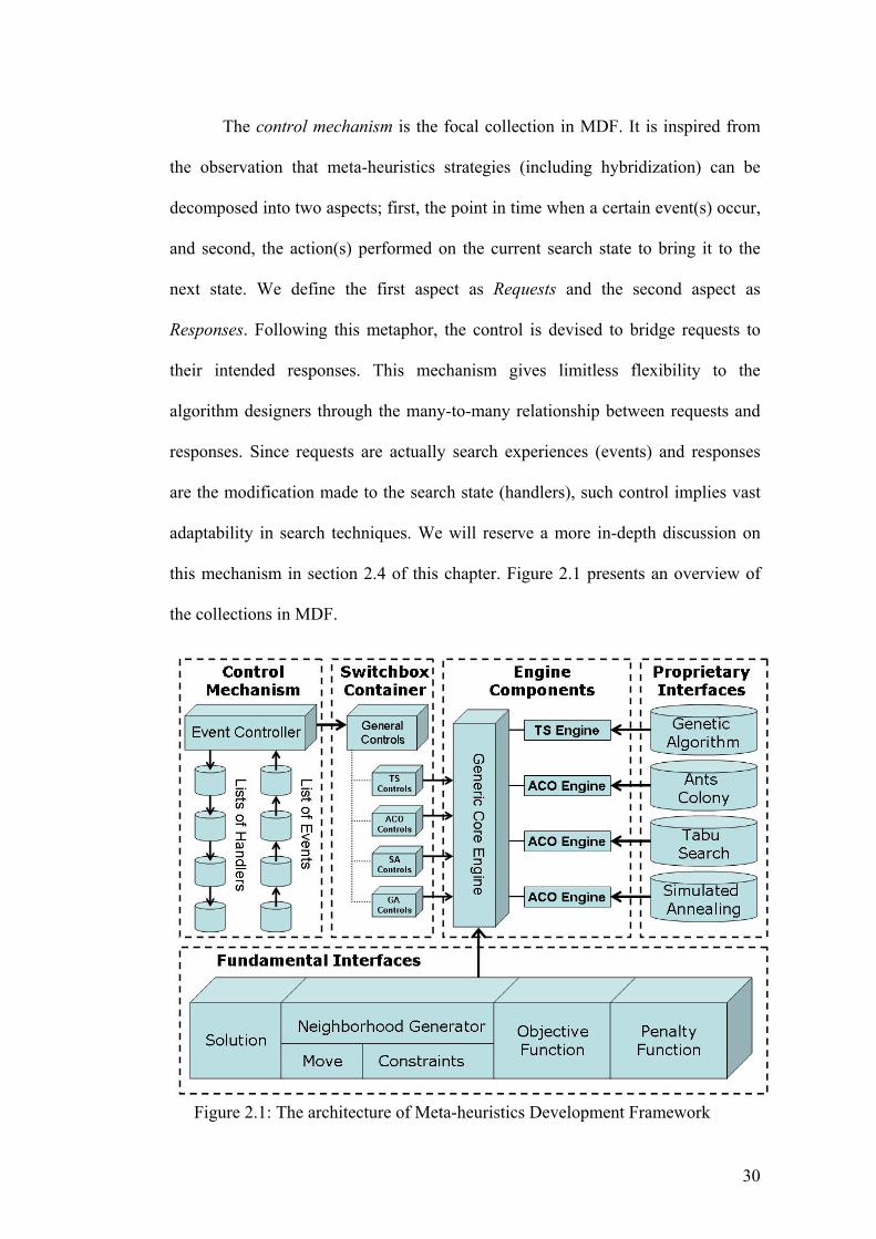
The control mechanism is the focal collection in MDF. It is inspired from

the observation that meta-heuristics strategies (including hybridization) can be

decomposed into two aspects; first, the point in time when a certain event(s) occur,

and second, the action(s) performed on the current search state to bring it to the

next state. We define the first aspect as Requests and the second aspect as

Responses. Following this metaphor, the control is devised to bridge requests to

their intended responses. This mechanism gives limitless flexibility to the

algorithm designers through the many-to-many relationship between requests and

responses. Since requests are actually search experiences (events) and responses

are the modification made to the search state (handlers), such control implies vast

adaptability in search techniques. We will reserve a more in-depth discussion on

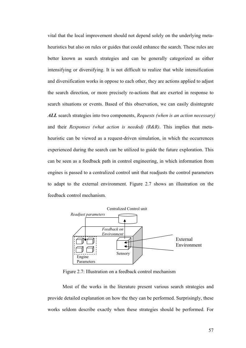
this mechanism in section 2.4 of this chapter. Figure 2.1 presents an overview of

the collections in MDF.

Figure 2.1: The architecture of Meta-heuristics Development Framework

30

MDF also incorporates a built-in software library that facilitates developing

selected strategies. While these generic strategies are not as powerful as some

specific methods that are tailored to a problem type, these components provide a

quick and easy means for fast prototyping. In the following sections, we will

explain and discuss each of these collections.

2.1 Fundamental Interfaces

The fundamental interfaces are intended to classify the common behaviors

of meta-heuristics into distinctive abstract classes. Figure 2.2 illustrates how this

common behavior can be formulated into the interfaces. For each interface, we will

present the virtual functions that are essential for the objects and a description of

their uses.

New State [Solution]

Evaluate State [Objective Function]

Apply Penalty [Penalty Function]

Generate Next State [Neighborhood Generator]

Check Feasibility [Constraint]

Translate to New State [Move]

Figure 2.2: The relationship of Meta-heuristics behavior and MDF’s fundamental interfaces

2.1.1 Solution Interface

Virtual Function:

• Solution* Clone ( void ); Function 1

Descriptions:

31

The Solution class provides a representation to the result of problem. MDF

imposes no restriction on the solution formulation or the type of data structures

used because the search engine never manipulates the Solution objects directly.

Instead, the engine relies on the Move object to translate the Solution, the Objective

Function object to evaluate the Solution and the Solution itself for cloning. The

Solution interface has one virtual function, Clone (Function 1), which returns a

cloned instance of the solution object. A pitfall for unaware programmer is the

common mistake of using shallow cloning (copy references of the data) instead of

deep cloning (copying the data itself) and by doing so, loses valuable results.

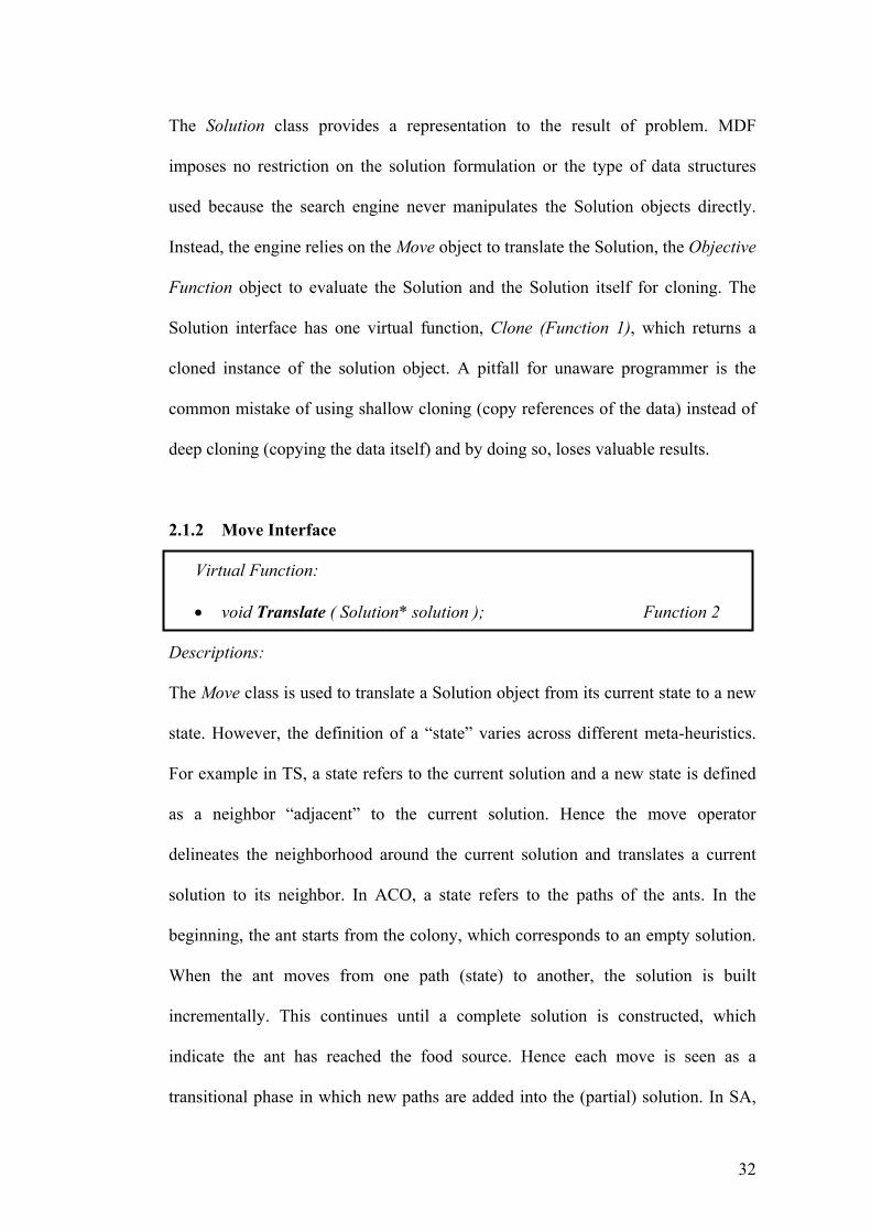
2.1.2 Move Interface

Virtual Function:

• void Translate ( Solution* solution ); Function 2

Descriptions:

The Move class is used to translate a Solution object from its current state to a new

state. However, the definition of a “state” varies across different meta-heuristics.

For example in TS, a state refers to the current solution and a new state is defined

as a neighbor “adjacent” to the current solution. Hence the move operator

delineates the neighborhood around the current solution and translates a current

solution to its neighbor. In ACO, a state refers to the paths of the ants. In the

beginning, the ant starts from the colony, which corresponds to an empty solution.

When the ant moves from one path (state) to another, the solution is built

incrementally. This continues until a complete solution is constructed, which

indicate the ant has reached the food source. Hence each move is seen as a

transitional phase in which new paths are added into the (partial) solution. In SA,

32

the move operator is a probabilistic operation that generates a random neighbor.

This definition of a state is similar to TS except that rather than a neighborhood,

only one neighbor in generated in each iteration. Finally in GA, the move operator

acts as a mutation to evolve the individuals (solutions). In this way, the current

state refers to the current generation and the new state is their offspring.

Surprisingly, there is no rule that prevents one meta-heuristic from using another’s

move. For example, TS could use ACO incremental move to build up a solution

and at the same time, tabu-ing the past constructed solution’s components to

prevent assembling the same solution (cycling) again. By adopting this view, it

becomes probable to assault problems at different angles and even instigate a new

technique. In addition, the interface also allows the multiple types of move for a

problem through inheritance. In VRPTW for example, both exchange and replace

moves can inherited the same Move interface. Beside moves that perform different

operation, it also implies that complex moves such as an adaptive k-opt can be

implemented to generate Very Large Scaled Neighborhood (VLSN). The Translate

function (Function 2) modifies the solution in its argument to its next state.

Programmer should be aware that the translate operation is permanent and cloning

should be done to prevent loss of solutions.

2.1.3 Constraint Interface

Virtual Function:

• int DegreeOfViolation ( Solution* solution, Move* move ); Function 3

Descriptions:

The Constraint class is usually used to ensure the feasibility of a solution. The

Degree of Violation function (Function 3) takes in two arguments, a solution and a

33

move objects and return an integer. The return parameter indicates “how much”

violation is presented in the candidate neighbor (i.e. neighbor = current solution ⊕

proposed move). A zero value signifies a feasible solution and any integer above

zero indicates infeasibility. It is possible to apply some relaxation criteria so that

violated solution can be accepted. This is extremely useful in oscillating strategies,

in which constraints are sometimes violated to explore previously inaccessible

regions and subsequently repaired. However, such tactics often run into the danger

of over-violation (solution can no longer to be repaired to feasibility) and a

restraint degree of violation can help to confine the risk.

2.1.4 Neighborhood Generator Interface

Virtual Function:

• Neighborhood* GenerateMove ( Solution* solution ); Function 4

Descriptions:

The Neighborhood Generator class generates the desired next states from the

current solution using the Generate Move function as shown in Function 4. When

the Neighborhood Generator is called, it will use the move objects to generate a list

of possible next states. It is possible to control the type of moves that is used to

generate the current neighbors. For example, if the search result is stagnant, the

Neighborhood Generator can be adjusted to generate drastic moves. This kind of

adaptive selection of moves can be easily programmed using MDF’s control

mechanism and hence guarantees a more controlled search process. After the

neighborhood is generated, the constraint objects select the candidates that satisfy

their criteria and these chosen candidates are recorded. The resultant neighborhood

is sent back for processing.

34

Each meta-heuristic has a different contextual meaning for the Neighborhood

Generator. For TS, the neighborhood generator produces a list of desired neighbor

with respect to the current solution. In ACO, the Neighborhood Generator

determines the possible subsequent paths that can be linked from the partial

solution. When no new path is constructed, it implies that the solution has been

completed built. In SA, the Neighborhood Generator acts as a generator for

generating the random moves and in GA, it performs the selection routine of

choosing the individuals for recombination. In short, the functionality of

Neighborhood Generator is to generate new candidates so that the meta-heuristics’

selection process could continue.

2.1.5 Objective Function Interface

Virtual Function:

• ObjectiveValueType Evaluate ( Solution* solution, Move* move ); Function 5

• boolean IsProposedBetterThanOriginal ( ObjectiveValueType proposed,

ObjectiveValueType original ); Function 6

Descriptions:

The Objective Function evaluates the quality of a solution. It uses a user-defined

metric called ObjectiveValueType to dictate favorableness of the solution. With

this design, implementer can now define their objective value type to an integer, a

double (floating point number) or even a vector of integer or double. This is

especially useful for goal programming optimization, in which there are several

objectives to be considered and inconvenient to be projected into a single

dimension. VRPTW for example has two objectives, which are to minimize the

number of vehicle used and the distance traveled. Sometimes, it is impractical to

35

project these two objectives of different dimension together (i.e. how much

distance is equivalence to the cost of a vehicle). In MDF, both objective values are

stored and compared independently, which allows a case-by-case evaluation.

In order to improve the performance of search, the Objective Function object also

supports incremental calculation. Absolute calculation should be done for the

initial solution and subsequently switched to incremental calculation for efficiency

reasons. An example on absolute and incremental calculation can be illustrated

using the Knapsack Problem (KSP). For the initial solution, the objective value is

calculated by adding up all the items’ values contained in the knapsack. This

method is known as the absolute calculation. Subsequent addition and removal can

be computed using incremental calculation from the original objective value by

adding or subtracting the targeted item value. The Evaluate function (Function 5)

is designed for this purpose and Is Proposed Better Than Original function

(Function 6) determines whether a proposed next state is better than current state.

2.1.6 Penalty Function Interface

Virtual Function:

• ObjectiveValueType ApplyPenalty ( Solution* solution, Move* move ObjectiveValueType NeighborObjectValue ); Function 7

Descriptions:

The Penalty Function gives a temporary penalty to the objective value. This is

extremely useful in implementing soft constraints. Typically soft constraints are

employed by the algorithm designer to incline the search toward preferred

solutions. For example in KSP, bricks and cements are encouraged to be packed

together unless the cost is very high and this user-constraint can be easily

36

implemented by applying a “bonus” (negative penalty) to solution value if such

arrangement occurred.

2.2 Proprietary Interfaces

This section addresses the interfaces that describe the behaviors exclusive

to each meta-heuristic. Interestingly, by formulating these unique behaviors into

abstract classes, it gives us valuable insights in forming innovative hybrids. For

example, a tabu list can be added to ACO to empower the ants with memory and

the annealing schedule can be added to GA as a breeding criterion. In addition,

algorithm designers can define their own proprietary interfaces that may mature

into a new technique.

Tabu Search

2.2.1 Tabu List Interface

Virtual Function:

• boolean IsTabu ( Solution* solution, Move* move ); Function 8 • void SetTabu ( Solution* solution, Move* move ); Function 9

Descriptions:

The Tabu List reduces the tendency of solution cycling through the use of memory.

The most straightforward implementation is to use a list that stored previously

visited solutions for the tenured duration. While this approach looks simplistic,

there are a few concerned issues. We consider the case of a solution size of l, a

tabu tenure t and running for k iterations and analyze the computational time. In

every iteration, each neighbor has to be verified with every element in the tabu list

37

and this requires Ο(l * t). Suppose there is an average of m neighbors in each

iteration, then the total computational time spent in validating the tabu status is O(l

* t * m * k). Apparently, the efficiency of the tabu list could be improved if one or

more of the four parameters is/are reduced. Since t and k directly affect the

algorithm effectiveness, they should be tuned optimality. As for m, it is sometimes

possible to reduce the size without sacrificing the quality (such as using a

candidate list strategy), but it is generally done heuristically and thus could not be

guaranteed. l is the best parameter to cut down as it is usually unnecessary to

record the complete solution. A possible approach is to record the hash of the

solution rather than the solution itself.

Unfortunately for some problems, it is sometimes impossible or very costly to

validate the tabu status even if the solutions are stored. For example in TSP,

solution A consisting of a tour of 1-2-3-4 and solution B of a tour of 2-3-4-1 can

only be detected as the same solution if rotational comparison is supported. Hence,

rather than tabu-ing the solutions, sometimes the move applied can be tabu-ed.

Typically, moves only affect some portions of a solution and thus occupy lesser

space then the solution. To reduce cycling, subsequent moves are verified to ensure

the reverse moves would not be applied. Apparently such technique does not

strictly prevent all forms of solution cycling in its tenure. Nevertheless it is

effective and generic to problems.

As oppose to tabu-ing the move, a more restrictive approach is to tabu the

objective value. This is based on the assumption that most solutions have an

unique objective value and thus tabu-ing the objective value is almost as good as

tabu-ing the solution itself. The drawback of this approach is that elite solutions

that have the same objective value would be missed.

38

The Tabu List interface supported various kind of tabu techniques (including those

that are not mentioned in this thesis) by manipulating the list indirectly through the

virtual functions Is Tabu (Function 8) and Set Tabu (Function 9). The Is Tabu

verifies if the neighbor is tabu-ed and Set Tabu sets accepted neighbors into the list.

2.2.2 Aspiration Criteria Interface

Virtual Function:

• boolean OverrideTabu ( Solution* solution, Move* move, ObjectiveValueType neighborObjectiveValue, SwitchBox* switchbox ); Function 10

Descriptions:

The aspiration criterion is used to override the tabu status of a neighbor if it meets

some criteria. For example, when the tabu list is used to tabu the move applied,

there is a possibility that good neighbors may be mistaken as tabu-ed solutions.

The aspiration criterion could then override the tabu status of a neighbor if its

objective value is better than the best-found solution. A virtual function Override

Tabu (Function 10) is used to perform the exemption.

Ants Colony Optimization

2.2.3 Pheromone Trail Interface

Virtual Function:

• double ExtractPheromone ( Solution* solution, Move* move ) Function 11

• void UpdateLocalPheromone ( Solution* localSolution ); Function 12 • void UpdateGlobalPheromone ( Solution* currentSolution,

Solution* localSolution ); Function 13

39

• void PheromoneEvaporation ( void ); Function 14

Descriptions:

The Pheromone Trail object is used to record the pheromone density on the paths.

The pheromone trails is one of the two parameters used to determine the

transitional probability of ants in choosing their paths. While the local heuristics

can be seem as the ant’s natural judgment in taking a trail, it is the pheromone

density on the trails that influences the ant to change its direction. Each of these

factors is assigned a weight, α and β for the pheromone trail and local heuristic

respectively. In particular, the probability of moving from node r to node s is given

generally by

⎪⎩

⎪⎨

⎧∈

= ∑∈

otherwise

rJsifsrsr

srsr

srpk

rJuk

k

0

)()],(.[)],([

)],(.[)],([

),()(

βα

βα

ητητ

Eqn 2.1

where τ(r,s) = pheromone for moving from node r to node s η(r,s) = local heuristics for moving from node r to node s

The pheromone trail τ is usually initialized to a fixed value across of the trails prior

to being used (Elitism Strategy), and the value it is initialized to, τ0, is usually

given by a generic “baseline” solution to the problem. This solution can be

evaluated using any constructing algorithm likes Greedy Algorithm, or even ACO

itself (using a generic pheromone trail initialized to any arbitrary value). τ0 is a

function of this initial solution. The value of τ(r,s) is retrieved using the Extract

Pheromone function (Function 11).

After each move is completed, the ant may choose to perform a local pheromone

decay or deposit. If no such action is performed, each of the ants in the iteration

40

will be non-collaborative and use only the pheromone trail at the beginning of the

iteration. While there are implementations without local pheromone updates with

good results, it was generally found that local pheromone update improves solution

quality. The logic is that unlike real-ants, the solver of an optimization problem

needs to traverse the best path once to record it, and implement other ways to

enforce this knowledge (global pheromone update). Meanwhile, it is necessary to

search as much of the solution space as possible, and in most cases, it is better to

lower the pheromone concentration from a taken trail, so that other ants may try

the less trodden paths, which leads to a more aggressive search around the

neighborhood as well as to prevent solution cycling. There are many formulas (if

implemented) for local pheromone update, but generally,

0.),().1(),( τρτρτ ll srsr +−← Eqn 2.2

where τ0 represents the default pheromone level ρl represents the local decay factor

Local pheromone update can be performed in two ways. The first, step-by-step

update is performed as each ant takes a move. The nature of this process makes it

more suited for a parallel implementation. The second, online-delayed pheromone

update, is performed as each ant completes a solution build, and is more suited for

a serial implementation. This process is updated by the ACO search indirectly

through the Update Local Pheromone function (Function 12).

While the local pheromone update may be optional, the global pheromone update

that occurred at the end of iteration is compulsory. The justification for such an

action is by counter-intuition. Suppose there is no pheromone update. Then, each

ant will repeatedly find the same probabilities on all the moves. The only variable

then is the random choice. While this progresses the solution, it does so very

41

gradually. Furthermore, there tend to be an excessive amount of solution cycling

due to the constant nature of the probabilities. This completes the intuition that the

pheromone trail should be updated. Global pheromone update can be performed in

several ways. Some implementations proposed using the trail from all the ants in

the iteration (AS, ASrank), others advocate using only the best route in the iteration

(MMAS, ACO), and most suggest using the best route found so far. Generally,

),(.),().1(),( srsrsr gg τρτρτ ∆+−← Eqn 2.3

where ρg represents the global decay factor

The global update on the pheromone trails is performed via the Update Global

Pheromone function (Function 13). In synch with global pheromone update is the

optional pheromone evaporation, which is updated with the Pheromone

Evaporation (Function 14). One idea is to use additional reinforcement for unused

movements, with equation 2.4, while other approaches perform a simple

evaporation on all trails with equation 2.5, for all i and j:

0.),(),( τρττ ejiji +← Eqn 2.4

),().1(),( jiji e τρτ −← Eqn 2.5

where ρe represents the evaporation factor

2.2.4 Local Heuristic Interface

Virtual Function:

• double ComputeLocalHeuristic ( Solution* solution, Move* move ) Function 15

Descriptions:

The Local Heuristic interface is used to incorporate the underlying heuristic in

solving the problem. Generally a single greedy heuristic is used for its speed and

42

performance. However there are instances of problems, especially those of

increased complexity that a single local heuristic does not suffice. For example,

there had been implementations of VRPTW with multiple combined local

heuristics [Bullnheimer et al., 1997]. In such instances, η(r,s) can be formulated as

∑=

=n

jj

jsrsr1

)],([),( αηη Eqn 2.6

where αj ≥ 0 and symbolize the weights of the local heuristics

The function Compute Local Heuristics (Function 15) is used to compute the value

of η(r,s), which is later used together with τ(r,s) as shown in Eqn 2,1 to give the

transitional probability.

Simulated Annealing

2.2.5 Annealing Schedule Interface

Virtual Function:

• double RetrieveCoolingTemperature ( Solution* solution, ObjectiveValueType neighborObjectiveValue SwitchBox* switchbox ) Function 16

Descriptions:

In SA, the probability of transition is a function of the objective values difference

between the two states and a global time-dependent parameter called the

temperature. Suppose δE is the difference in objective values of the current

solution and its neighbor, and T is the temperature. If δE is negative (i.e., the new

neighbor has a better objective value) then the algorithm moves to the new

neighbor with probability 1. If not, it does so with probability e-δE/T. This rule is

deliberately similar to the Maxwell-Boltzmann distribution governing the

distribution of molecular energies. It is clear that the behavior of the algorithm is

43

crucially dependent on the T. If T is 0, the algorithm is reduced to greedy, and will

always be moving toward a neighbor with a better objective value. If T is ∞, it

moves around randomly. In general, the algorithm is sensitive to coarser objective

variations for large T and finer variations for small T. This is exploited in designing

the annealing schedule, which is the procedure for varying T with time (the number

of iterations). At first T is set to infinity, and is gradually decreased to zero

("cooling"). This enables the algorithm to initially get to the general region of the

search space containing good solutions, and later hone in on the optimum. The

Annealing Schedule Object is catered for algorithm designer to devise their cooling

function. The Retrieve Cooling Temperature function (Function 16) retrieves the

time-dependent T, when a non-improving neighbor is encountered.

Genetic Algorithm

2.2.6 Recombination Interface

Virtual Function:

• void Crossover ( Solution * parentA, Solution* ParentB Solution* offSpring1, Solution * offSpring2) Function 17

Descriptions:

The Recombination object combines the selected individuals to produce their

offspring. It incorporates a single tunable variable probability of crossover (P )c ,

which encodes the probability that two selected individual will actually breed.

Generally the value is set between 0.6 and 1.0. For each pair of parent, a random

number between 0 and 1 is generated. If the number falls under the crossover

threshold, the organisms are reproduced or otherwise, they are propagated into the

next generation unchanged. Crossover results in two new child individuals, which

44

are added to the next generation pool. The Crossover function shown in Function

17 is dictated for this purpose. During the crossover, the chromosomes of the

parents are mixed typically by simply swapping a portion of the underlying data

structure, although other more complex merging mechanisms have proved useful

for certain types of problems. This process is known as one-point crossover and is

repeated with different parent individuals until there are an appropriate number of

candidate solutions in the next generation pool.

2.2.7 Population Interface

Virtual Function:

• void InitializeFirstGeneration ( void ) Function 18 • void DiscardUnfitIndividuals ( void ) Function 19

Descriptions:

GA solution is usually represented as simple strings of data in a manner not unlike

instructions for a von Neumann machine, although a wide variety of other data

structures for storing chromosomes have also been tested, with varying degrees of

success in different problem domains. The Population object is used to keep a

collection of such individuals, with each new population (generation) created at the

end of every iteration. Initially a first generation population is seeded unto the

gene pool. This function is implemented in the Initialize First Generation function

(Function 18) and is used by the Population object to initialize the individuals prior

to the start of the algorithm. The first generation can be created randomly or by

heuristics such as randomized greedy. However, it is vital that the implementer

ensures the diversity of the first generation to prevent rapid convergence of similar

individuals. To prevent over-population, GA employs various strategies in

45

selecting the individuals for the next generation (Fitness Techniques, Elitism,

Linear Probability Curve, Steady Rate Reproduction). To cater for these strategies,

the Population object uses the Discard Unfit Individuals (Function 19) that mixes

parents and their children together and consequently discards some of these

individuals in accordance to the user-specific strategies.

2.3 Engine and its Component

Section 2.1 and 2.2 has illustrated the various abstract classes in MDF. In

this section, we observe how the MDF search engines put these classes together

and then discuss on the issues arising from the integration. This section also

provides the opportunity to examine the search parameters (contained in the engine

switch box) and analyze their effects on the search process.

2.3.1 Engine Interface

Virtual Function:

• void StartSolving (void ) Function 20 • void StopSolving ( void ) Function 21

• Solution* GetBestFoundSolution ( void ) Function 22

Descriptions:

The Engine Interface contains the general operations that are subsequently

inherited by the meta-heuristics engines. There are three operations, Start Solving

(Function 20) that begins the search sequences, Stop Solving (Function 21) that

terminates the search and Get Best Found Solution (Function 22) that returns the

best found solution in the search. These virtual functions prevent unnecessary

46

amendment to application codes when an implementer changes the underlying

meta-heuristic, thus giving a more generic design.

2.3.2 Switchbox Interface

Parameter:

• NumberOfIteration Parameter G1

Descriptions:

The Switchbox interface complement the Engine interface as a container that stores

the generic parameter presented in meta-heuristics. The Number Of Iteration

(parameter G1) indicates the amount of time the meta-heuristics is allowed to run

and is often used as a termination criterion. Typically, the quality of solutions

improves with the increasing number of iterations, which follows the law of

diminishing returns. As such, it is important to determine a value that gives

sufficiently well results and yet be computed in a reasonable time. Unfortunately,

there are many factors that affects this variable and they include the problem size,

the meta-heuristics’ parameters (such as tabu tenure, pheromone density), the

strategies involved (internsification/diversification) and even instances of the

problem. Hence it is a challenge for an algorithm designer to devise an

optimization scheme that could produce the best results in the fastest possible time.

2.3.3 TS Engine

TS Engine performs the rudimentary procedures of TS and the pseudo-code

is presented in Figure 2.3. Prior to the search, TS Engine initializes a solution

usually from a problem-specified constructing heuristic.

47

TS Engine

procedure

Initialize a current Solution

while terminating criteria not reached

Neighborhood Generator generates a new neighborhood;

Constraint discards any undesired neighbors;

Objective Function evaluates selected neighbors;

Penalty Function applied to neighbors;

Tabu List and Aspiration Criteria are consulted;

Move translates current Solution to best neighbor;

if new Solution is better than best found Solution

Clones and records new Solution as best found Solution;

end if

Tabu List is updated;

end while

end procedure

Figure 2.3: The TS Engine Procedure (pseudo-code)

Based on this solution, the Neighborhood Generator creates a list of neighbors

using the Move object(s). The Constraint object(s) then validate each of these

created neighbors to select a subgroup of accepted neighbors, which are also

known as candidates. These candidates are then evaluated using the Objective

Function. The Penalty Function is applied to the objective value of the candidates

and the best non-tabu neighbor is selected after consulting the Tabu List and

Aspiration Criteria. At this point, a new state is selected and the selected Move

object translates the current solution to the chosen neighbor. The objective value of

the new solution is compared against the best-found solution and if the value is

48

better, the new solution will be cloned and then recorded. Finally the Tabu List will

be updated to prevent reoccurrence of solutions. If the terminating condition is not

reached at this time, a new neighborhood will be generated and the iterative search

continues.

2.3.4 TS Switchbox

Parameter:

• Tabu Tenure Parameter TS1 • First Accept Parameter TS2

Descriptions:

The Tabu Tenure (Parameter TS1) determines the tabu-ed duration of visited

solution. Apparently a short tenure is ineffective in preventing solution cycling and

a long tenure requires a greater validating time. In fact it is almost impossible to

find an optimal tenure value even for instances of a same problem. Hence a

popular approach is to vary the tenure in accordance to the search events. This

strategy is known as reactive tabu list and is illustrated in Control Mechanism.

There are several ways to implement the tabu tenure. An effectual implementation

is to set up the tabu list is a circular array with size equals to the tenure. In this way,

when the list is filled, the first inserted solution will be replaced. Beside the tenure,

TS Engine also uses First Accept (Parameter TS2). Typically, TS will examine

each candidate in the neighborhood to determine the best neighbor to move to.

However, when time is crucial (such as real-time optimization), it is possible to

speed up the search by accepting the first encountered neighbor with an improving

objective value. This strategy is known as first-accept and can be activated by

setting the First Accept parameter to true.

49

2.3.5 ACO Engine

ACO Engine performs the rudimentary procedures of ACO and the pseudo-code is

presented in Figure 2.4. Using the Elitism Strategy, the pheromone trail is first

updated with pre-constructed solution(s).

ACO Engine

procedure

Initialize the Pheromone Trail

while terminating conditions not reached

while there is still ants in colony and

while the solution is not completed

Neighborhood Generator generates a set of new trails;

Constraint discards any impassible trails;

Trail chosen by consulting Local Heuristic and Pheromone Trail

Move translates the Solution with selected trail;

Local Pheromone Trail Updated

End while

end while

Objective Function evaluates solutions constructed by ants;

Penalty Function is applied to determine the quality of solutions;

Global Pheromone Trail is updated;

If new Solution is better than best found Solution

Clones and records new Solution as best found Solution;

end If

Pheromone Evaporation Occurred;

end while

end procedure

Figure 2.4: The ACO Engine Procedure (pseudo-code)

50

ACO Engine then uses a triple nested loop to carry out the ACO routines. The

main procedure performs the iterative improvement steps bounded by the number

of iteration or user-defined criteria. The colony procedure (second loop) spawns

the activity of each ant in the colony and updates the global pheromone trails in

accordance to the defined strategies (such as ASrank, MMAS or ACO). In addition

to the global pheromone update, the colony procedure also executes the pheromone

evaporation. The innermost loop describes the ant activity in constructing a

solution. The Neighborhood Generator generates the ant’s trails with respect to the

ant current position (partial solution). The Constraint objects then obstruct the

trails that would lead to infeasible solution. The transitional probability of each

trail is computed by consulting the Local Heuristic and Pheromone Trail, and the

ant randomly chooses a path with this probability. When a trail is selected, the

Move object adds the new trail into the partial solution. Optional local pheromone

update strategies such as ACO, is applied to improve the search and the activity

continues until the solution is completely built.

2.3.6 ACO Switchbox

Parameter:

• Number of Ants Parameter ACO1 • α (Pheromone Trail weight) Parameter ACO2 • β (Local Heuristic weight) Parameter ACO3 • ρ (Decay factors) Parameter ACO4 • q0 (Exploitation/Exploration factor) Parameter ACO5

Descriptions:

There are many arguments on the optimal number of ants and the two most agreed

value for this parameter (Parameter ACO1) is a constant value (e.g., 10) or n

51

(problem size) [Bullnheimer et al., 1997; Dorigo et al., 1996]. The impact of a

choosing n will increase the computational complexity of the problem by another

factor of n. Based on x iterations and n2 for the probability calculation, choosing a

constant number of ants give O(xn2), whereas n ants gives O(xn3). However more

ants could mean better exploration. Hence, both arguments are valid, and the

decision on the value should be up to the implementer. Another two important

parameters are the weights value of α (Parameter ACO2) and β (Parameter ACO3).

[Dorigo, 1992] found from experimental results that good values of α and β (for

TSP at least) are 1 and 5 respectively. A greater weight is usually placed on the

local heuristics (affected by β) to prevent fast convergence to local optimal.

Another key parameters are the decay factors ρ (Parameter ACO4). These factors

are generally set between 0 and 1, to signify the percentage of decay/evaporation

(0 means no decay, 1 means complete decay). Decay factors can be subdivided into

three separate parameters (local decay, global decay, and evaporation), although

most classic ACO uses the same value for them. Exploration or exploitation factor

is another important factor in the ACO algorithm. A complete exploitation reduce

the algorithm simply to the power of the local heuristics, in most cases just a

greedy approach. Exploration allows an opportunity to search around the best-

found solution, a technique that works often in non-linear problems. The decision

of exploration or exploitation is defined by the factor q0 (Parameter ACO5) the

exploitation factor, which has a domain of 0 to 1. When q0 is 0, the ants explore all

the time; when q0 is 1, exploitation occurs all the time.

2.3.7 SA Engine

52

SA Engine performs the rudimentary procedures of SA and the pseudo-code is

presented in Figure 2.5. Similar to TS and ACO, an initial solution is created as the

starting point of the search.

SA Engine

procedure

Initialize a current Solution;

while terminating conditions not reached

Neighborhood Generator generates a random neighbor;

Constraint validates the feasibility of neighbor;

Objective Function evaluates solutions;

Penalty Function temporary adjusts the objective value;

If new neighbor is better than current Solution

Move translates Solution to neighbor;

Else

Consults the Annealing Schedule;

If neighbor is accepted

Move translates Solution to neighbor;

Else

Current Solution remains unchanged;

end if

end If

If new Solution is better than best found Solution

Clones and records new Solution as best found Solution;

end If

end while

end procedure

Figure 2.5: The SA Engine Procedure (pseudo-code)

53

The Neighborhood Generator then generates a random Move and this neighbor is

evaluated with the Objective Function. The Penalty Function is the applied to the

neighbor’s objective value and the adjusted value is then compared against the

current solution. If the objective value of the neighbor is better, the Move object

translates the current solution to its neighbor. Otherwise, the annealing schedule is

speculated to see if the non-improving neighbor could be accepted. If the neighbor

is accepted, the Move object will translate the solution; otherwise, the current

solution will remain unchanged. This procedure is repeated until the any of the

terminating criteria is reached.

2.3.8 SA Switchbox

Parameter:

• Temperature Parameter SA1

Descriptions:

There are various approaches in modeling the temperature and can be classified as

either static or dynamic. In a static annealing schedule, the parameters are fixed

and cannot be changed during the execution. In this category, there are two simple

static annealing schedules. The first schedule is the exponential cooling scheme

(ECS), which has the form of Tk+1 = αTk, where α is some constant that satisfies 0

< α < 1, k is the annealing schedule index starting from 0, and T0 is the initial

temperature. This cooling is first proposed by [Kirkpatrick et al., 1983] with α =

0.95. Another cooling scheme is the linear cooling scheme (LCS) [Randel and

Grest, 1986], which has the form of Tk+1 = Tk - ∆T (i.e. T is reduced for every L

trials).

54

2.3.9 GA Engine

GA Engine performs the rudimentary procedures of GA and the pseudo-code is

presented in Figure 2.6.

GA Engine

procedure

Initialize the first generation Population;

while terminating conditions not reached

Neighborhood Generator selects Solutions for mating;

Recombination crosses selected Solutions to form new children

Constraint discards infeasible children;

Move mutates feasible children;

Objective Function evaluates children;

Children are mixed into the parent Population;

Penalty Function adjusts the objective value of all Solutions in Population;

Population discards unfit individuals until the population is balanced;

If any Solution in Population is better than best found Solution

Clones and records new Solution as best found Solution;

end If

end while

end procedure

Figure 2.6: The GA Engine Procedure (pseudo-code)

Initially, the Population object creates the first generation pool. From this gene

pool, the Neighborhood Generator selects the individuals (Solutions) for crossover.

The developer specifies the type of crossover and implements in the

Recombination object. When the crossover is performed, the Constraint objects

validate the offspring to ensure their feasibility. The Move objects

55

translates/mutates the qualified Solutions so as to improve their fitness, which is

evaluated by the Objective Function. The mutated children are mixed with their

parents and the Penalty Function is applied to the whole population. The

Population is now over-populated and some of the solutions are discarded based

on the modified objective value until the number of solutions is the same as the

original population. Subsequently the new population is used to generate the next

generation and this procedure is repeated until any of the terminating conditions is

reached.

2.3.10 GA Switchbox

Parameter:

• Pc (probability of crossover) Parameter GA1

Descriptions:

Pc (Parameter GA1) is an optional parameter that determines the probability in

which two selected individuals are combined. For most GA application, Pc is often

set as 1 (i.e. all selected individuals are mated successfully). However, this implies

that elite individuals (which have high selection probability) may lose their “good”

traits during the crossover or mutation. Hence the primarily function of Pc is to

probabilistically preserve some elite parents for each successive generations. It is

also possible to model this parameter in accordance to the SA annealing schedule.

2.4 Control Mechanism

The objective of the Control Mechanism is to allow the meta-heuristic to

adapt itself with the various situations that occurred during a search process. As

meta-heuristics suffer from the inability of performing global optimization, it is

56

vital that the local improvement should not depend solely on the underlying meta-

heuristics but also on rules or guides that could enhance the search. These rules are

better known as search strategies and can be generally categorized as either

intensifying or diversifying. It is not difficult to realize that while intensification

and diversification works in oppose to each other, they are actions applied to adjust

the search direction, or more precisely re-actions that are exerted in response to

search situations or events. Based of this observation, we can easily disintegrate

ALL search strategies into two components, Requests (when is an action necessary)

and their Responses (what action is needed) (R&R). This implies that meta-

heuristic can be viewed as a request-driven simulation, in which the occurrences

experienced during the search can be utilized to guide the future exploration. This

can be seen as a feedback path in control engineering, in which information from

engines is passed to a centralized control unit that readjusts the control parameters

to adapt to the external environment. Figure 2.7 shows an illustration on the

feedback control mechanism.

Centralized Control unit

Feedback on Environment

Readjust parameters

Engine Parameters

Sensory

External Environment

Figure 2.7: Illustration on a feedback control mechanism

Most of the works in the literature present various search strategies and

provide detailed explanation on how the they can be performed. Surprisingly, these

works seldom describe exactly when these strategies should be performed. For

57

example in the work of [Stutzle and Dorigo, 1999], the importance of exploitation

and exploration is illustrated together with a recommended value for q0. The

authors also proposed how q0 can be dynamically changed but failed to provide

exact details on the factors affecting q0. The same predicament surfaced in [Battiti

and Tecchiolli, 1994], in which the authors could not present accurate rules that

could guide the behavior of the reactive tenure. Obviously, these authors could not

be faulted as we realize the considerable efforts involved in coming up with precise

rules, especially when some of these rules are problem-specified. However, it

would be interesting if we could input different rules into their works and observe

their effects. The control mechanism facilitates this by providing an experimental

“playground” that could readily convert user-defined rules into program codes.

Rules are turned into search events (Requests) and the techniques are converted

into handlers (Responses) and a “multiple-to-multiple” relationship can be

established between these components.

Most interestingly, the R&R concept provides a suitable platform for

forming hybridized models. Most meta-heuristic hybrids are either loosely coupled

such as the two phase approach (e.g. [Maa and Shanblatt, 1992], [Gehring and

Homberger, 2001]) or with one meta-heuristic embedded on another [Stutzle and

Dorigo, 1999]. We observe that in these hybrids, each meta-heuristic occupies a

certain time phase in the search. These phases can be rotated (loosely coupled

hybrids) or interpolated (embedded hybrids). We define an atomic unit as the

smallest unit time for a meta-heuristic to perform a completed set of routine and

assign each phase as an atomic unit. Due to the diverse nature of meta-heuristics,

the definition of an atomic unit varies across them. In most cases, an atomic unit is

equivalent to one search iteration but in techniques like ACO, an atomic unit

58

means the activity of a single ant. Table 2.1 shows the definition of an atomic unit

in TS, ACO, SA and GA. Once the search process is partition into atomic units,

each of these units is allocated to a meta-heuristic. The allocation can be adaptive

to the previous events and the assigned meta-heuristic is dependent on the rules set

by the algorithm designer.

Table 2.1: The definition of an atomic unit in TS, ACO, SA and GA

Meta-heuristics Atomic Unit Definition

Tabu Search An iteration of the search

Ant Colony Optimization The activity of an ant

Simulated Annealing Generating a new random move

Genetic Algorithm A new generation

In our model, a search state at any atomic time point comprises of the best-

found solution, the current solution, the current operating meta-heuristic and the

values of search parameters at that point. Prior to the search, the algorithm designer

inputs the requests (or rules) that react to event(s) such as improving solutions,

non-improving solutions, new best solution found and end of atomic unit. A search

algorithm begins with an initial search state. As the search proceeds, any occurred

event(s) that matches the rules of the requests will be activated, which

consequently triggered the desired responses. Suppose we are solving a problem

using TS and we implement a response that performs “switch the operating meta-

heuristic to SA” and a request that states “execute the switch if 100 non-improving

moves are encountered”. In this example, each time the search process notices a

non-improving solution, the request will be informed. When a hundred non-

improving solutions are encountered, the request will trigger the response, which in

turn changes the operating meta-heuristic from TS to SA. In the next section, we

59

will examine how the R&R can be implemented using three mechanisms, Events,

Handlers and Event Controller.

2.4.1 Event Interface

Virtual Function:

• list <EventMessage> TriggerResponse ( Engine* currentEngine ) Function 23

Descriptions:

The Event object implements the user-defined rule(s) in a request. When the

operating engine detected an event that matches these rules, the Trigger Response

function (Function 23) will evoke a list of required action (Event Message). Each

of these messages is associated with two parameters: the response to be executed

and its corresponding priority. There are three priority levels, namely, (a)

INSTANT, which is to execute the responses immediately, (b) NORMAL, which

is to execute the responses at the end of the atomic unit, and (c) DELAYED, which

is only executed after all the responses with priority NORMAL have been

performed. The hierarchical nature of the priority queue will allow designers to

have additional control over sequence of responses.

2.4.2 Handler Interface

Virtual Function:

• void Execute ( EventController* eventController ) Function 24

Descriptions:

The Handler object implements the responses that readjust the search procedure.

Generally these responses can be classified into two categories, parameters-based

60

and techniques-based strategies. Parameters-based strategies such as reactive tabu

search and dynamic annealing schedule adapt their search parameters in

accordance to events. An example could be a reactive tabu list that shortens the

tabu tenure when an elite solution is encountered and lengthens it when there is

solution cycling. For this strategy, two Handler objects are required, with one

object handling increment and the other decrement. When an event (such as an

elite solution) is encountered, the Handler will modify the parameter(s) in

Switchbox via the Event Controller using the Execute function (Function 24).

Techniques-based strategies on the other hand, usually modified parts of the search

state. Modifications include changing the current solution, the underlying meta-

heuristic and/or the search procedure (e.g. intensification/diversification). These

modifications can be evoked using the Event Controller, who has control to every

aspect of the search state.

2.4.3 Event Controller

The role of the Event Controller is to control the search process through the

adjustment of search state, which includes the current operating meta-heuristic

engine, the search parameters and the current solution. In software term, it acts as

an interface between the user-defined requests and the meta-heuristics engine.

Initially, the Event Controller sets up the search engine. As the search proceeds,

events experienced such as the behavior of the solutions’ objective values, the

structure of the solutions are recorded. This information is compared against the

user-defined request. If there is a match, the related responses are queued and later

triggered according to their priority. The Event Controller also assures that

duplicate responses would not be triggered twice in the same atomic time.

61

2.4.4 Further Illustrations

Our first example illustrates how MDF performs hybridization using the

“request and response” paradigm. The illustrated hybrid scheme is proposed by

[Stutzle and Dorigo, 1999], in which ACO and Local Search (LS) were hybridized

to solve TSP. The authors’ approach was to apply LS to the iteration-best solution

before the ants update it into the pheromone trails. This strategy is implemented in

MDF as follows; ACO is the operating meta-heuristic and LS is embedded as a

Handler, which we will denote as the LS handler. We define a request

(End_ACO_Event) that will be triggered at the end of every ACO search iteration

and set it to NORMAL priority. When an iteration is completed, this event will

register a match with the request and the Event Controller will execute the LS

handler. The LS handler then modifies the search state by applying LS onto the

iteration best solution. Subsequently, the enhanced solution will be updated into the

pheromone trail for future ants. Figure 2.8 shows the code fragment of the

End_ACO_Event and LS handler as an illustration of this technique-based strategy.

class End_ACO_Event : Event {

list<EventMessage>TriggeredResponse ( Engine* This )

{ If ( This->IterationCompleted ( ) )

list.add (“LS Hander”, NORMAL); return List;

} }

class LS_hander : Handler { void Execute(EventController* This) {

TSP_Solution* currentBestSoln = This->GetCurrentSolution(); LSEngine->SetInitialSolution(currentBestSoln); LSEngine->StartSolving(); This->SetCurrentSolution (LSEngine->GetBestFoundSolution()); } }

Figure 2.8: An illustration on a technique-based strategy

62

Our next illustration is on reactive tabu search, in which we show how

parameter-based strategies can be implemented using MDF. Reactive tabu search

refers to strategies that adaptively adjusting tabu search parameters according to

the search trajectory. Many complex heuristics have been proposed with this

strategy, each with its own assumptions on the solution space. In fact a popular

analogy is to visualize the solution space as a multi-dimensional terrain. The

factors include objective value, similarity in the solution structure and time. Based

on these factors, the reactive tabu search attempts to navigate along the terrain

toward new local optima. In order to simplify our illustration, we only consider

two factors, time and objective value and the parameter adjusted is limited to the

tabu tenure. Time simply refers to number of iterations performed. Our simplified

strategy works as follows. When we encounter a series of non-improving we

lengthen our tabu tenure so as to prevent solution cycling. On the other hand, when

we encounter a new best solution, we shorten our tenure in order to perform

intensification. We implement an event called Reactive_Event which trigger two

handlers, Lengthen_Tenure and Shorten_Tenure. The first handler

(Lengthen_Tenure) will increase the tabu tenure by some x amount when the search

encounters a series of non-improving moves. On the other hand, when a new best

solution is encountered, we will revert back the tenure, discarding any move that

have been kept for more than n iterations using the Shorten_Tenure handler. The

code fragment for this implementation is shown in Figure 2.9.

63

class Reactive_Event : Event {

Int countBadMove = 0; int badMoveLimit = n; // Maximum allowed bad moves

bool TriggeredResponse( Engine* This ) { If ( This->BestSolutionFound( ) ) {

list.add ( “Shorten_Tenure” , NORMAL ); countBadMove = 0; } Else { If ( countBadMove = badMoveLimit ) list.add ( “Lengthen_Tenure”, NORMAL );

Else countBadMove ++; } } } class Shorten_Tenure : Handler { void Execute(EventController* This) { This->SBContainer->TSSwitchBox->TabuList.Tenure = t; } } class Lengthen_Tenure : Handler { void Execute(EventController* This) { This->SBContainer->TSSwitchBox->TabuList.Tenure = t + x; } }

Figure 2.9: An illustration on a parameter-based strategy

64

2.5 Software Strategy Library (SSL)

SSL provides a list of tools that facilitates some of the more popular

strategies. For example, the two static annealing schedules (exponential and linear)

are incorporated. These tools can be classified as tools for general strategies and

for specific meta-heuristics such as the discussed annealing schedules. SSL

remains an on-going work due to the numerous strategies (both existing and new)

that can and would be included. Sections 2.5.1 and 2.5.2 provides more

illustrations on the SSL components.

2.5.1 General Tools Illustration: Elite Recorder

SSL supports this strategy by storing a list of elite solutions during the

search in the Elite Recorder. Each of these elite solutions can be used as a new

initial solution for another meta-heuristic. The rationale is to search these elite

solutions more intensively and perhaps differently across various meta-heuristics.

The Elite Recorder is embedded as a Handler and is triggered when a new best

solution is found.

2.5.2 Specific Tools Illustration: Very Large Scaled Neighborhood (VLSN)

VLSN [e.g. Ahuja et al., 2003] works on the principle that by generating a larger

neighborhood, it increases the chances of obtaining better solutions. One approach is to

repetitively apply the Move operator “k times” on all the neighbors generated in each move.

However, to prevent the neighborhood from expanding exponentially, it is often useful to

select only the elite neighbors to narrow down the size. SSL provides a Candidate List

class that inherits from the Constraint Interface. It selects the best n neighbors from those

generated by each k-opt moves.

65

CHAPTER 3

APPLICATIONS SURVEY

This chapter reviews some of the MDF applications published in the

literature. These applications include the Traveling Salesman Problem (TSP), the

Vehicle Routing Problem with Time Window (VRPTW) and the Inventory Routing

Problem with Time Window (IRPTW). The choice of TSP, VRPTW, and IRPTW is

a generalization of many real-world routing problems, which tend to have multiple

objectives and constraints. For instance, the IRPTW considers inventory costs

across multiple period of VRPTW, which in turn is the VRP extended with time

window, which in turn is extended with optimal fleet (vehicles) size objective from

the classic and NP-hard TSP. The extensions of NP-hard problems with more

constraints and objectives provide increasing approximate analogy to practical

application, increasing the value of solving these problems optimally. As such,

these problems are chosen to demonstrate the power of re-use in the framework in

solving similar or extended instances of a problem. By logic of induction, the MDF

framework would be applicable for re-use in other problems as long as a solution

can be formulated for the base problem.

3.1 Traveling Salesman Problem (TSP)

The Traveling Salesman Problem is a classic NP-hard problem, and the

mathematical basis related to TSP was treated as earlier as the 1800s by the Irish

mathematician Sir William Rowan Hamilton and the British mathematician

Thomas Penyngton Kirkman. [Held and Karp, 1969] provides a look at the TSP

and the related Capacited Minimum Spanning Tree, while [Biggs et al., 1976]

66

provides discussion on the works on the afore-mentioned mathematicians. The

development of the general form of TSP, as well as other classic combinatorial

optimization problems, is studied by [Schrijver, 1960]. While the problem was

well-known, there appears a lack of reference in the literature to earlier work, and

it was not until 1954 that the most popular TSP definition came from [Dantzig et

al., 1954]. TSP definitions for general and variant forms of the problems are easily

available. In the context of this thesis, TSP is defined in Figure 3.1.

Let

G = (V,A) be a graph,

where V{ v1, v2, ... , vn } be a set of cities (vertex set), and

A = { (vi,vj) : vi,vj ∈ V, i ≠ j } be the edge set,

C(r,s) = C(s,r) be a cost measure associated with edge (r,s) w.r.t. A.

Figure 3.1: Problem definition of the Traveling Salesman Problem

A tour is defined as a Hamiltonian circuit passing exactly once through

each point in vertices V. The TSP objective is to find a tour of minimum

costs/distance. Interested reader can find the full historical mathematical

formulations of TSP at [http://rodin.wustl.edu/~kevin/dissert/node11.html], and

([Finke et al., 1984], [Lawler et al., 1985], [Naddef and Rinaldi, 1991], [Naddef

and Rinaldi, 1993]).

3.1.1 Design Issues

This section illustrates on the capability of MDF in supporting different

schemes of hybridization and presented in the work of [Lau et al.1, 2004]. The

authors use ACO and TS to exploit on various hybridization schemes in solving the

67

TSP. Their implementation, denoted as Hybrid Ant System and Tabu search

(HASTS), is a flexible hybrid method that spawns derived models that utilize the

strength of meta-heuristics adept at solving certain problems. Particularly, HASTS

takes advantage of the ACO for its nature capability as a constructing heuristic and

TS as a local improvement heuristic. By varying the degree of importance of the

inherent algorithms, various derived models are easy formed and formulated with

MDF.

The intrinsic flexibility and potential for collaboration allows HASTS to

vary the importance of the component meta-heuristics. ACO and TS are argued to

be good complements to each other, as ACO works using a preference list, given

by the pheromone trail, while TS operates using a forbidden (or tabu) list. The

algorithmically opposite techniques offered a high potential that when one

algorithm reaches a local optimal, the other algorithm has a higher chance of bring

it out and improving the solution henceforth.

HASTS improves results by adjusting the importance level and degree of

collaboration of the component meta-heuristics in the hybrid technique, via the

framework provided by MDF. Each variant of HASTS has a set of algorithms as

the core algorithm, while the other algorithm(s) serves as the aide algorithm(s).

Each of these variant becomes a derived model of HASTS. The advantage of the

derived models lies in the ability to adapt search to exploit the strength and cover

the weakness of the meta-heuristics under the scheme. As such, HASTS is

especially suitable for solving complex problems through the use of a divide-and-

conquer approach, by first breaking down and identifying the objectives of the sub-

problems, and solving them using the best approach optimally. This aptitude will

be illustrated in the next two sections, VRPTW and IRPTW. For this section, we

68

focus on illustrating the effects of different hybrids on TSP and observe the efforts

required to construct each of them. Figure 3.2 showed four possible derived

models of HASTS.

(A) HASTS-EA (B) HASTS-IE

(C) HASTS-ED (D) HASTS-CC

Figure 3.2: The four derived models of HASTS

The four derived models are respectively Empowered Ants (HASTS-EA)

(Figure 3.2(A)), Improved Exploitation (HASTS-IE) (Figure 3.2(B)), Enhanced

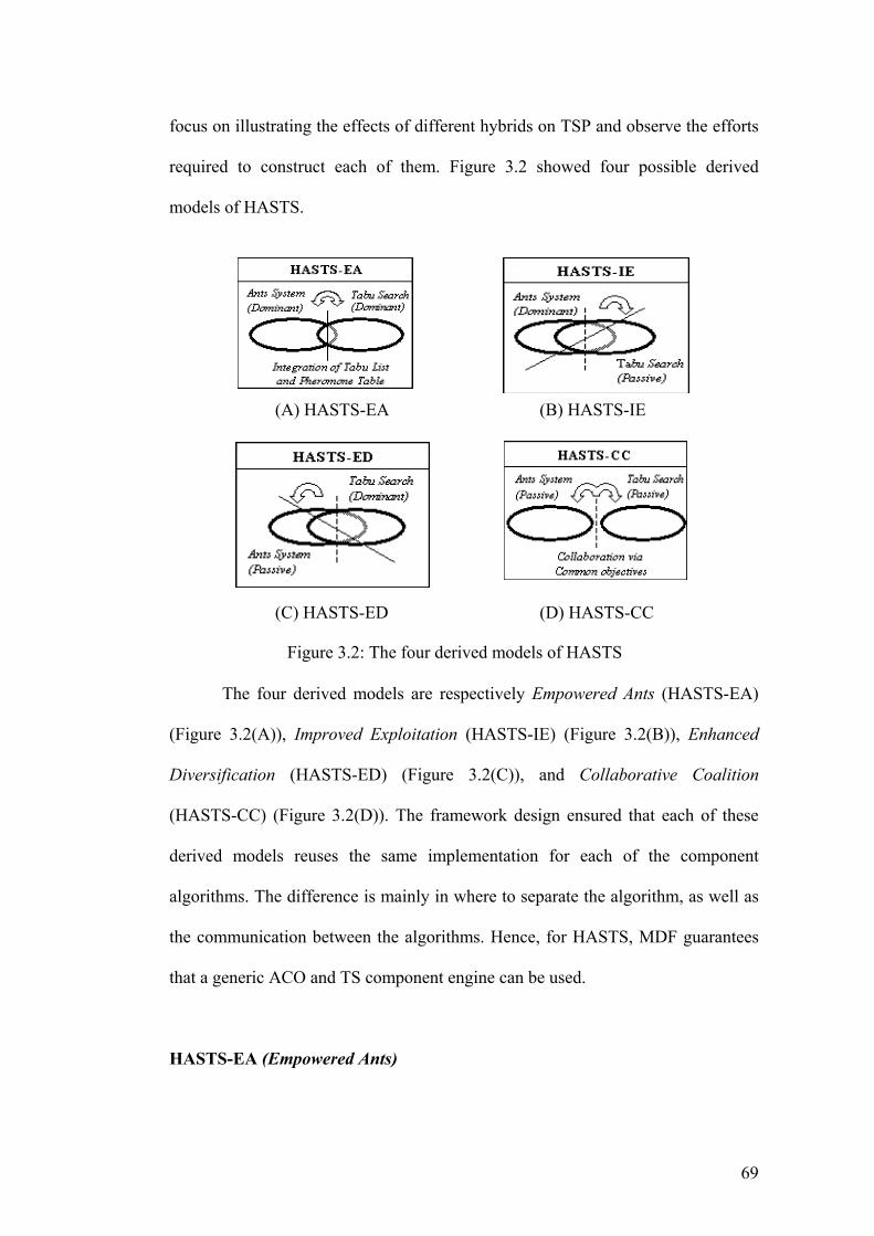
Diversification (HASTS-ED) (Figure 3.2(C)), and Collaborative Coalition

(HASTS-CC) (Figure 3.2(D)). The framework design ensured that each of these

derived models reuses the same implementation for each of the component

algorithms. The difference is mainly in where to separate the algorithm, as well as

the communication between the algorithms. Hence, for HASTS, MDF guarantees

that a generic ACO and TS component engine can be used.

HASTS-EA (Empowered Ants)

69

This derived model arises from the observation that when ACO reaches

local optimal solutions, it suffers from a tendency of solution cycling in the near

optimum region due to their emphasis on the strong pheromone trails. By

empowering the ants with memory, it reduces the chances of reconstructing the

same solution. An analogy can be drawn where each ant becomes more intelligent

to find a better trail by not following false tracks laid by previous ants. Following

this metaphor, ACO optimizes the solution based on its pheromone trails as a

“preference” memory, while solution cycling is reduced via the tabu list.

Furthermore, TS can be applied to diversify the solutions radically, hence

encouraging exploration that helps to escape from local optimality. The tabu list

also eliminates the need for local pheromone decay, which reduces one of the

parameters. This implementation, however, suffers from a slight increase in

computational needs, as well as more computational memory for the additional

tabu list. This tradeoff however, is often justified by the increase in performance,

especially over large iterations. From an implementation viewpoint, HASTS-EA

modifies ACO to include a tabu list, which records the solution made by each ant

in a single iteration. Subsequently, each ant in the iteration would check if the next

move is tabu-ed. If it is, the move will be dropped and a new move will be

generated. The tabu list is reset at the end of the iteration. Figure 3.3 shows the

pseudo-code of HASTS-EA.

70

71

procedure: HASTS – EA () while (termination-criterion-not-satisfied) while (Max_Ant_Not_Reached) Ants_generation_and_activity Pheromone_Evaporation Reset_Tabu_List Daemon_actions end Schedule_activities end while

end procedure

procedure: Ants_generation_and_activity () while (available_resources) Schedule_creation_of_new_ant New_Solution = New_active_ant update_Tabu_List (New_Solution)

end while end procedure procedure: New_active_ant () Initialize_ant; M = read_Pheromone Trail T = read_Tabu_List while (current_state != target_state) A = read_local_ant_routing_table P = compute_transitional_probabilities (A, M) for Next_state do Next_state = apply_ant_decision_policy(P) end for while (check_Tabu_List (Next_state) == non-tabued) Move_to_next_state (next_state) if (online_step-by-step_pheromone_update) Deposit pheromone Update M end if end while

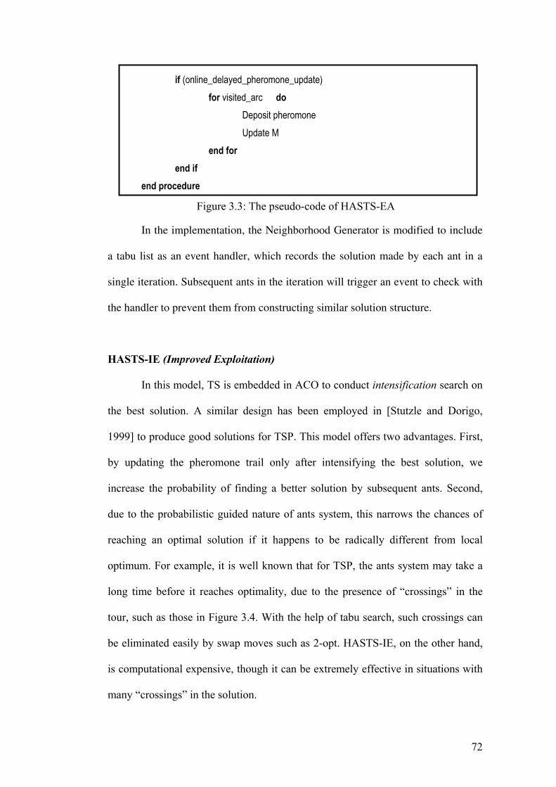
if (online_delayed_pheromone_update) for visited_arc do Deposit pheromone Update M end for end if end procedure

Figure 3.3: The pseudo-code of HASTS-EA

In the implementation, the Neighborhood Generator is modified to include

a tabu list as an event handler, which records the solution made by each ant in a

single iteration. Subsequent ants in the iteration will trigger an event to check with

the handler to prevent them from constructing similar solution structure.

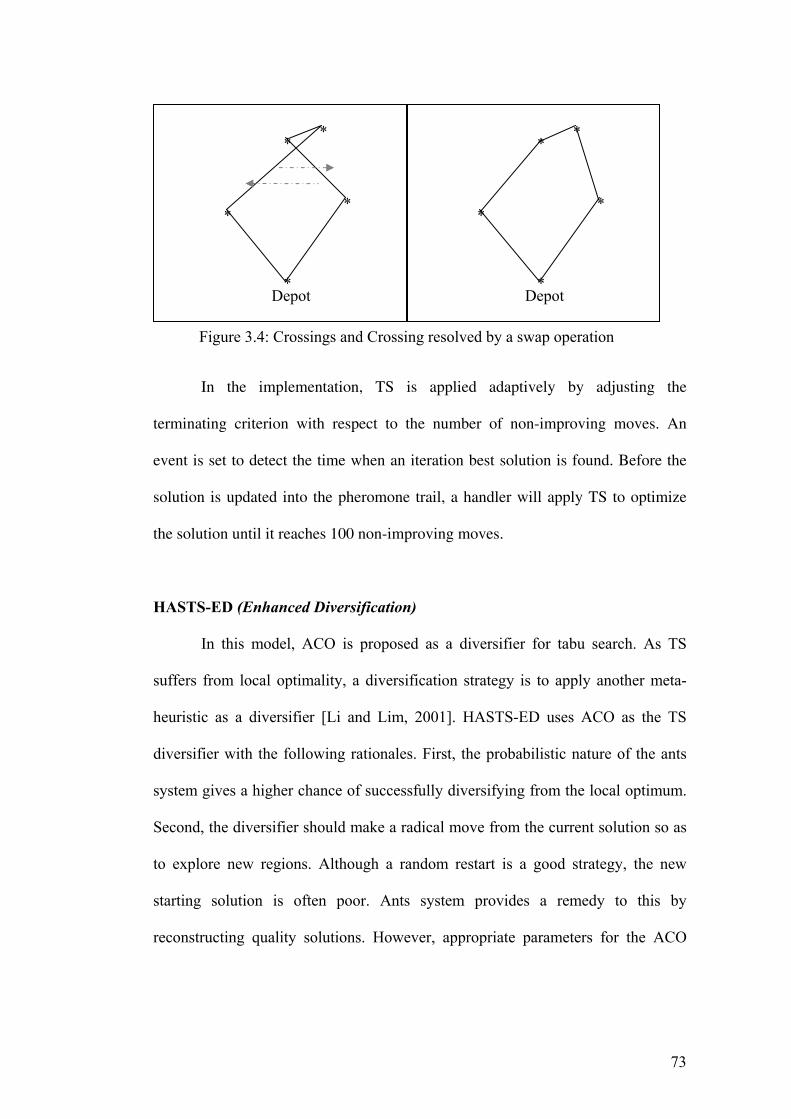
HASTS-IE (Improved Exploitation)

In this model, TS is embedded in ACO to conduct intensification search on

the best solution. A similar design has been employed in [Stutzle and Dorigo,

1999] to produce good solutions for TSP. This model offers two advantages. First,

by updating the pheromone trail only after intensifying the best solution, we

increase the probability of finding a better solution by subsequent ants. Second,

due to the probabilistic guided nature of ants system, this narrows the chances of

reaching an optimal solution if it happens to be radically different from local

optimum. For example, it is well known that for TSP, the ants system may take a

long time before it reaches optimality, due to the presence of “crossings” in the

tour, such as those in Figure 3.4. With the help of tabu search, such crossings can

be eliminated easily by swap moves such as 2-opt. HASTS-IE, on the other hand,

is computational expensive, though it can be extremely effective in situations with

many “crossings” in the solution.

72

* ** *

In the implementation, TS is applied adaptively by adjusting the

terminating criterion with respect to the number of non-improving moves. An

event is set to detect the time when an iteration best solution is found. Before the

solution is updated into the pheromone trail, a handler will apply TS to optimize

the solution until it reaches 100 non-improving moves.

HASTS-ED (Enhanced Diversification)

In this model, ACO is proposed as a diversifier for tabu search. As TS

suffers from local optimality, a diversification strategy is to apply another meta-

heuristic as a diversifier [Li and Lim, 2001]. HASTS-ED uses ACO as the TS

diversifier with the following rationales. First, the probabilistic nature of the ants

system gives a higher chance of successfully diversifying from the local optimum.

Second, the diversifier should make a radical move from the current solution so as

to explore new regions. Although a random restart is a good strategy, the new

starting solution is often poor. Ants system provides a remedy to this by

reconstructing quality solutions. However, appropriate parameters for the ACO

*Depot

**

*

**

Depot

Figure 3.4: Crossings and Crossing resolved by a swap operation

73

diversifier should be set, such as a low q0 that is unusually in most other effective

ACO implementation.

In the implementation, a counter event is used to adaptively apply ants to

diversify as a non-linear function of non-improving moves. A recommended

function is to cumulatively increment the number of non-improved move tolerated

for every diversification applied. The diversification technique is embedded into

the handler, which reconstructs the part of best-found solution in TS using ACO.

HASTS-CC (Collaborative Coalition)

HASTS-CC proposes a collaborative coalition between the ACO and TS.

This model offers the least coupling between the two meta-heuristics but allows

great flexibility in the formulation of the problem. One configuration of HASTS-

CC is to espouse the two-phase approach as advocated by [Schulze and Fahle,

1997]. This approach consists of a construction phase follow by an optimization

phase. ACO work extremely well for the construction phase as it could be used

independently to obtain quality solutions. Being an optimization heuristic, tabu

search fit naturally into the second phase of the approach. Such collaboration

exploits the natural heritage of each meta-heuristic.

For the implementation, an event is set to switch from ACO to TS when

ACO has completed its intended iterations.

Hyper-hybrid models

In addition to the four hybrid schemes, [Lau et al.1, 2004] also illustrates

the ability of MDF in combining hybrid to hyper-hybrid. The authors introduce

two hyper-hybrid schemes, HASTS-CCED and HASTS-IEEA. HASTS-CCED

74

replaces the TS in HASTS-CC to HASTS-ED. This aims to enhance the optimizing

phase. For HASTS-IEEA, it fuses the tabu list strategy in HASTS-EA to HASTS-

IE, thus allowing HASTS-IE to develop a more aggressive diversifying capability.

HASTS-CCED and HASTS-IEEA are simple illustrations of how hyper-hybrids

can be easily formed from previously constructed hybrids when MDF is applied.

Initial experimentation of these hyper-hybrids has shown promising results with

low additional development cost.

3.1.2 Experimental Observations and Discussion

We demonstrate experimentally the cost-effectiveness of MDF in

hybridization. The TSP test problems are obtained from TSPLIB [Reinelt, 1991].

Development Cost of Hybrids

The most obvious and necessary incentive for using a framework is cost-

savings in development time. However, it is difficult to measure accurately the

amount of resources required as it is subject to numerous factors. The metric used

in [Lau et al.1, 2004] is to record the lines of code, which reveals partially the

programming efforts. Unfortunately, the number of lines of code alone is often

inadequate to reflect exact development time, as some programmers are known to

write condensed codes. In addition, this metric only considers the implementation

time and not the validation time. Intuitionally, if each hybrid scheme were

developed independently, they would have to be validated separately. An implicit

benefit of MDF is the reduction in validation cost. Usually the time required to

validate an application increases non-linearly with the amount of code. Hence the

savings could be considerable especially in complex applications such as meta-

heuristic hybridization. Figure 3.5 approximates the metric for each model. From

75

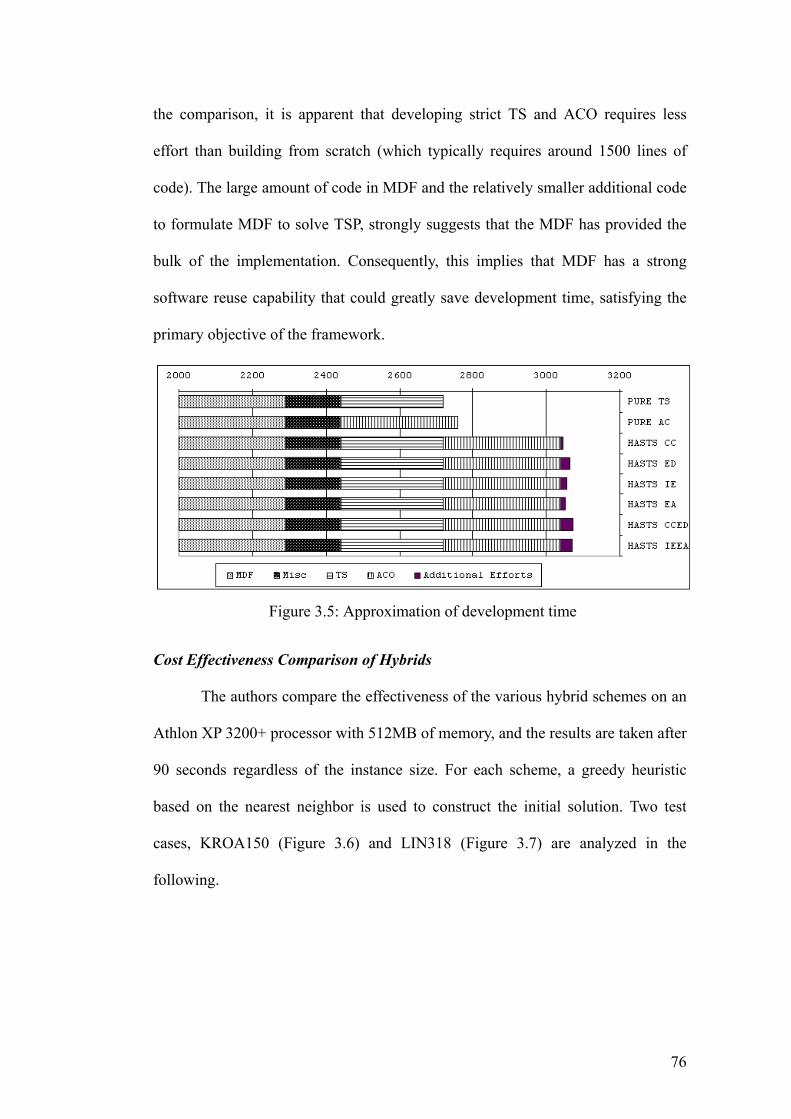
the comparison, it is apparent that developing strict TS and ACO requires less

effort than building from scratch (which typically requires around 1500 lines of

code). The large amount of code in MDF and the relatively smaller additional code

to formulate MDF to solve TSP, strongly suggests that the MDF has provided the

bulk of the implementation. Consequently, this implies that MDF has a strong

software reuse capability that could greatly save development time, satisfying the

primary objective of the framework.

Figure 3.5: Approximation of development time

Cost Effectiveness Comparison of Hybrids

The authors compare the effectiveness of the various hybrid schemes on an

Athlon XP 3200+ processor with 512MB of memory, and the results are taken after

90 seconds regardless of the instance size. For each scheme, a greedy heuristic

based on the nearest neighbor is used to construct the initial solution. Two test

cases, KROA150 (Figure 3.6) and LIN318 (Figure 3.7) are analyzed in the

following.

76

Figure 3.6: Result of test case KROA150

In test case KROA150, we observed that Pure TS converged faster then

Pure AC. However the solution quality of TS stops improving at around 10

seconds while Pure AC continued to improve on its solution. HASTS-CC, HASTS-

ED and HASTS-CCED produced the same result at 90 seconds although HASTS-

ED converged the fastest. Although HASTS-CCED appeared to be slowest to reach

the local optimum, we observe a rapid improvement from 22nd seconds to the 26th

seconds. The winner of this instance is HASTS-IEEA where the local optimum is

77

reached at 88 seconds. HASTS-EA has the weakest result showing the unsuitability

of the scheme in this instance.

Figure 3.7: Result of test case LIN318.

In test case LIN318, Pure AC could not improve significantly on the initial

solution. This phenomenon has been observed by the authors in [Stützle and

Dorigo, 1999], which comments that Pure AC does not solve TSP well for large

instances. Due to the weakness of Pure AC, HASTS-CC and HASTS-CCED are

rendered ineffective. Fortunately, the TS component compensates the weakness to

78

produce results that are comparable with Pure TS. HASTS-ED also produces result

close to Pure TS due to the ineffectiveness of the diversifier. The HASTS-IEEA

emerged as the winner although HASTS-IE is only a step behind. Again, we see

that HASTS-EA has little improvement as it was greatly affected by the limitation

of Pure AC.

In addition, another 13 test cases from the TSPLIB are recorded in Table

3.1. The “Bound” column shows the best-published results to date. Each column

gives the objective value and the percentage gap when compared with best-

published results. In summary, the table shows that HASTS-IEEA produces the

best results and has the best standard deviation. Although it is not conclusive, we

have a strong belief that hybrids usually out-perform their parents. Hence, with

MDF, complex hybridized schemes are now possible to be developed in much less

development time, allowing hybridization to become a practical solution for

algorithm improvement.

Table 3.1: Results for TSP from TSPLIB test cases Name Bound Pure TS Pure ACO HASTS-EA HASTS-IE Att48 10628 10755 1.19 10847 2.06 10860 2.18 10628 0.00ei151 426 427 0.23 430 0.94 430 0.94 427 0.23Pr76 108159 109186 0.95 111994 3.55 111435 3.03 108159 0.00kroA100 21282 21296 0.07 21559 1.30 22092 3.81 21282 0.00kroB100 22141 22235 0.42 23145 4.53 22936 3.59 22220 0.36Wil101 629 629 0.00 649 3.18 638 1.43 629 0.00Ch130 6110 6196 1.41 6492 6.25 6492 6.25 6124 0.23kroA150 26524 27125 2.27 27682 4.37 27621 4.14 26550 0.10kroB150 26130 26178 0.18 27909 6.81 28499 9.07 26132 0.01d198 16780 15909 0.82 17397 10.25 17213 9.08 15780 0.00kroA200 29368 29487 0.41 34087 16.07 35859 22.10 29565 0.67kroB200 29437 30121 2.32 36980 25.62 36980 25.62 29813 1.28a280 2579 2669 3.49 3157 22.41 3157 22.41 2598 0.74Lin318 42029 43123 2.60 52156 24.10 50053 19.09 42777 1.78pcb442 50778 52025 2.46 61979 22.06 61979 22.06 51873 2.16STD Deviation 1.11 9.15 9.13 0.70

79

Name Bound HASTS-ED HASTS-CC HASTS-CCED HASTS-IEEA Att48 10628 10628 0.00 10653 0.24 10628 0.00 10628 0.00ei151 426 426 0.00 426 0.00 426 0.00 426 0.00Pr76 108159 108159 0.00 108159 0.00 108159 0.00 108159 0.00kroA100 21282 21282 0.00 21282 0.00 21292 0.05 21282 0.00kroB100 22141 22210 0.31 22200 0.27 22271 0.59 22141 0.00wil101 629 629 0.00 629 0.00 629 0.00 629 0.00ch130 6110 6128 0.29 6150 0.65 6113 0.05 6113 0.05kroA150 26524 26767 0.92 26727 0.77 26762 0.90 26525 0.00kroB150 26130 26152 0.08 26860 2.79 26391 1.00 26130 0.00d198 16780 16876 0.61 15796 0.10 15799 0.12 15781 0.01kroA200 29368 29668 1.02 29487 0.41 29603 0.80 29479 0.38kroB200 29437 30121 2.32 30121 2.32 30121 2.32 29543 0.36a280 2579 2658 3.06 2669 3.49 2654 2.91 2579 0.00lin318 42029 42938 2.16 43123 2.60 43083 2.51 42665 1.51pcb442 50778 51860 2.13 52025 2.46 51955 2.32 51654 1.73STD Deviation 1.05 1.26 1.07 0.56

3.2 Vehicle Routing Problem with Time Windows (VRPTW)

The Vehicle Routing Problem [Toth and Vigo, 2002] is a generic class of

complex combinatorial optimization problems extended from the TSP and the Bin

Packing Problem (BPP), and was first formulated by [Dantzig and Ramser, 1959].

The VRP is a generalization of the TSP, with additional m constraints, the m-TSP,

inductively making VRP NP-hard. Inversely, the TSP is the VRP with one un-

capacitated vehicle (which is the elementary version of VRP, the Capacitated

Vehicle Routing Problem – CVRPT), no depot, and customers with no demand.

Such observation inspired some approach to solving VRP using a divide and

conquer method to break VRP into several Multiple TSP (MTSP, a TSP with m

identical duplicated origin and m salesman) (e.g., [Bullnheimer et al., 1997]). VRP

and its variations had been well examined and solved using various techniques

from exact methods (e.g., [Baldacci et al., 1999], [Balinski and Quandt, 1964],

[Christofides and Eilon, 1969], [Christofides et al., 1981], [Cook and Rich, 1999],

[Cullen et al., 1981], [Fisher, 1988], [Fisher and Jaikumar, 1981], and [Foster and

80

Ryan, 1976]), to heuristics and meta-heuristics (e.g., [Braysy, 2001], [Chiang and

Russell, 1997], [Cordeau et al., 2000], [Gillet and Miller, 1974], and [Rousseau et

al., 1999]).

A popular and important variant to the VRP, the Vehicle Routing Problem

with Time Windows (VRPTW), introduce additional constraints to the original

definition, specifying that each costumer must be served within a specific time

window. Other variants of the problem are multi-depot, fixed routes, fixed areas,

etc. Such variants are formulated as they better approximate practical scenarios.

This thesis in particular looks at VRPTW, which is defined in Figure 3.8.

Let

G = (V, A) be a graph,

where V = {v0, v1, … , vn} is the vertex set, and

A = {(vi, vj) | vi, vj ∈ V, i ≠ j} is the edge set.

Figure 3.8: Problem definition of the Vehicle Routing Problem with Time Windows

This definition is similar to the TSP definition. The difference is in the

additional constraints. The depot vertex v0, has m identical vehicles, each with a

maximum load capacity Q and a maximum route duration D. The remaining vertex

vi є V represent customers to be serviced, each with a non-negative demand qi, a

service time si, and a service time window comprised of a ready time ri and a due

time li. A waiting time wi is incurred if customer i is serviced before its ready time.

Each edge (vi, vj) has an associated non-negative costij, interpreted as the travel

time tij between location i and j. A complete tour is defined by the order in which

the n customers are serviced by m vehicles, and the objective of VRPTW is to

determine a complete tours starting and ending at the depot, such that each

81

customer is visited exactly once within its time window, the total demand of any

vehicle route does not exceed Q, the duration of any vehicle route does not exceed

D and the total cost of all routes is minimized.

Due to the number of constraints in the problem, there are many definitions

on the problem optimality. A widely debated factor is whether to consider distance

or number of vehicles as the primal optimality factor, with more researchers

focusing on the latter as the primary factor with the former as the secondary factor,

due in part to the challenge among the community in solving [Solomon, 1987]

benchmark test cases. ([Larsen, 1999], [Mester, 2002], and [Mester and Braysy,

2002]) provides further references on the VRPTW.

3.2.1 Design Issues

The problem being solved in this instance, the VRPTW, is an NP-hard

multi-objective optimization problem. Traditional approach in solving VRPTW

involves projecting all objectives into a single dimension. However, the correlation

between these various objectives are usually weak and difficult to express using a

common aspect. In addition, during the search, the optimizer has no insight to

which objective it is improving. This resulted in redundancy spent in optimizing

the secondary objectives while the primary objective is being optimized. To

resolve this, an approach is to optimize the problem by independently considering

each of its objectives, allowing precise strategies to be employed. In solving this

problem, a decision can be made to decompose the problem into the following

objectives:

82

Objective 1: Minimize the number of vehicles given a set number of customers.

The dual problem is to maximize the total number of customers

given a set of vehicles.

Objective 2: Minimizes the total distance traveled given a fixed set of vehicles.

This divide-and-conquer formulation suggests the suitability of using

HASTS. As had been mentioned earlier, each derived model of HASTS share the

same implementation for the component algorithm. It is also seen that VRPTW is

an extension of the TSP. Hence, in the implementation, HASTS utilizes a generic

ACO and TS implementation for TSP, and reuse this implementation with

modifications to handle the additional constraints in VRPTW, to provide a solver

for VRPTW. This solver is then extended by each derived model, and modified

according to the specifications of the sub-problem it is assigned to solve. Figure

3.9 shows the evolution of the MDF implementation in solving VRPTW using

HASTS.

HASTS derived model 1

HASTS derived model n

VRPTW solver TSP solver

Figure 3.9: Codes reuse for MDF implementation

For this problem, HASTS requires only two derived models, HASTS-IE

and HASTS-ED described earlier. The first objective can be reformulated to its

dual model and writing it as maximizing the customers served in given a set of

vehicles, and reduce the required vehicles each time a solution that serves all the

83

customers is found with the lesser fleet size. The HASTS-EA derived model is

appropriate for this sub-problem. ACO is a good meta-heuristic for this objective

as it optimizes the solution quality through reconstruction. TS, although possible,

is not a suitable candidate as it tries to ‘pull’ the solution to feasibility through

optimizing the customers’ sequence in the tour, which is a slow process. Instead,

tabu search is used to empower the ant system by intelligently rupturing the

pheromone trails left by the ants, and in doing so, helped the ants from being

ensnared in a local optimum. Initially m vehicles are obtained by applying a greedy

heuristic to serve all customers. The algorithm then reduces the value of m by 1

and seeks to construct a feasible solution that services all the customers. Once a

feasible solution is found, the number of vehicles is reduced to the best-found

number of vehicles and the process is repeated for a new feasible solution. This

sub-problem requires the search to find a configuration where the customers can fit

into the pre-set vehicles. HASTS-EA performs well since the tabu list assists each

ant in an iteration to construct a radically different solution. Although other derived

models can also be used, they lack of the intensified exploration that HASTS-EA

provides.

Objective 2 is attempted after Objective 1 had been optimized, and as a

result, this sub-problem will consist of a tighter solution space. In spite of the

success by HASTS-EA in optimizing the number of vehicles, this derived model is

not very effective for this objective because of the difficulties involved in

constructing different feasible solutions on an allowed number of vehicles due to

the nature of ACO. Instead, another derived model, HASTS-ED, is employed to

minimize the total distance on a fixed set of vehicles. HASTS-ED uses tabu search

as the core heuristic with ants system acting as the diversifier. Tabu search is

84

effective in solving this sub-problem as it optimizes the route distance rather than

reconstructs the solutions. However, tabu search still faces the danger of being

entrapped in a local optimum during its search. To address this issue, when tabu

search encounters a local optimum, it randomly selects some of the routes to be

reconstructed by ACO, which assists tabu search by radically re-configuring the

selected partial routes. Details on this objective relies mainly on the operations of

Tabu Search and is examined in further detail in [Lau et al.2, 2003].

3.2.2 Experimental Observations and Discussion

VRPTW, as mentioned, as extended from the TSP. The classical and most

common comparison for VRPTW solvers in the literature is with the Solomon’s

VRPTW benchmark [Solomon, 1987], consisting of a total of 56 test cases

covering different scenarios. These test cases included a set of problems consisting

of Clustered nodes (C101-C109, and C201-208), which generally is best solved by

assigning vehicles to service the same or nearby clusters in the problem; a set of

problems consisting of Random nodes (R101-R112, and R201-R211), which has

nodes randomly assigned, and solving it optimally will be problem specific; and a

set of problems consisting of a combination of Random and Clustered nodes

(RC101-108, and RC201-208). Table 3.2 tabulates the results obtained.

Table 3.2: Results for VRPTW from the Solomon’s original test cases (n=100)

Test cases TS ACO HASTS

C101 10/828.94 10/855.07 10/828.94 C102 10/852.97 10/1072.24 10/845.61 C103 10/858.62 10/1435.26 10/840.88 C104 10/856.87 10/1182.64 10/857.57 C105 10/828.94 10/936.47 10/828.94 C106 10/828.94 10/958.91 10/828.94 C107 10/828.94 10/877.99 10/828.94 C108 10/828.94 10/1033.81 10/828.94

85

C109 10/828.94 10/1900.94 10/828.94 R101 19/1686.24 19/1929.05 19/1686.24 R102 18/1518.93 18/1886.77 18/1493.31 R103 14/1301.64 14/1679.71 14/1301.64 R104 11/1072.04 10/1198.69 10/1025.38 R105 14/1459.84 14/1651.43 14/1458.60 R106 13/1324.38 12/1564.99 12/1314.69 R107 11/1165.87 10/1144.72 10/1140.27 R108 10/1002.56 10/1117.25 10/ 994.66 R109 12/1287.62 12/1502.57 12/1207.58 R110 11/1218.33 11/1348.78 11/1166.65 R111 11/1104.93 11/1239.53 11/1172.66 R112 10/1039.55 10/1242.24 10/1041.36 RC101 15/1742.29 15/1899.97 15/1698.50 RC102 13/1605.30 13/1780.98 13/1551.32 RC103 11/1337.04 11/1567.12 11/1371.40 RC104 11/1249.13 10/1353.87 10/1187.97 RC105 15/1633.39 14/1899.54 14/1618.01 RC106 12/1428.88 12/1620.67 12/1434.33 RC107 12/1312.84 11/1468.59 11/1266.92 RC108 11/1258.40 10/1326.94 10/1273.12 C201 3/591.56 3/ 591.56 3/ 591.56 C202 3/591.56 3/ 993.62 3/ 591.56 C203 3/617.32 3/1065.81 3/ 605.23 C204 3/673.46 3/1046.87 3/ 594.80 C205 3/604.67 3/ 913.03 3/ 588.88 C206 3/632.35 3/ 647.29 3/ 588.49 C207 3/621.02 3/ 646.69 3/ 588.49 C208 3/588.88 3/ 646.72 3/ 588.49 R201 4/1308.84 4/2048.31 4/1366.34 R202 4/1123.34 3/1755.11 3/1239.22 R203 3/1013.59 3/1625.26 3/1000.29 R204 3/817.60 3/1159.14 3/ 781.86 R205 4/1022.02 3/1678.53 3/1063.29 R206 4/963.94 3/1525.34 3/ 955.34 R207 3/863.60 3/1258.12 3/ 866.35 R208 3/761.94 2/1016.07 2/1016.07 R209 4/934.45 3/1551.01 3/ 979.30 R210 3/1000.53 3/1659.90 3/ 968.32 R211 3/816.33 3/1143.96 3/ 865.51 RC201 4/1704.92 4/2226.23 4/1445.00 RC202 4/1265.78 4/1878.00 4/1204.45 RC203 3/1118.19 3/1706.48 3/1091.71 RC204 3/884.70 3/1342.81 3/ 826.27 RC205 4/1435.06 4/2271.26 4/1469.25 RC206 4/1162.96 3/1717.62 3/1259.12 RC207 4/1178.01 3/1733.47 3/1127.19 RC208 3/931.76 3/1422.07 3/ 937.78

86

Table 3.2 is read as follows: TS refers to the results obtained using a

standard Tabu Search implementation on MDF-TSF. ACO refers to the results after

passing the data through derived model HASTS-EA, a predominantly ACO

technique implemented with MDF-ACF that focus on solving the first objective

(minimizing the fleet size of vehicles). Finally, the HASTS column tabulates the

results obtained after the entire HASTS process mentioned earlier – in effect after a

combination of HASTS-EA and HASTS-ED.

Note the effectiveness of the hybrid HASTS compared against TS and

ACO, which adequately showed the effectiveness of MDF and a divide and

conquer hybrid approach. Also, the results from TS are generally better than ACO

in this instance due to the different objectives of the approach. TS has an objective

of minimizing distance, and perform it so well that for some instances, such as

R202, it performs better in terms of distance, but is worse off by the problem

definition specifying the fleet size as primary priority, while the ACO results

focuses mainly on reducing the fleet size of vehicles. It should also be further

noted that the development of the TS implementation takes about 3 months man-

hours, while the ACO implementation takes a lesser amount of time at about 2

months, due to its simpler nature. Meanwhile, with the availability of MDF,

HASTS requires only less than a week man-hours to develop.

3.3 Inventory Routing Problem with Time Window (IRPTW)

The Inventory Routing Problem with Time Window (IRPTW) follows as a

natural extension from the VRPTW, with the additional constraint over multiple

time-periods, which better reflect practical scenarios of a known future period

planning. Despite the complexity, literature survey showed that IRPTW can be

87

solved optimally if major restrictions are imposed. [Carter et al., 1996] proposed a

Lagrangean heuristic to solve a single-supplier, single-warehouse instance of the

problem, but it is sensitive to the values of several parameters where there are no

good heuristics for setting them, and is unable to guarantee feasibility. [Chan et al.,

1998] modeled a single-item, constant demand distribution system and presented

worst case as well as probabilistic bounds. However, it is doubtful that any of the

asymptotically optimal heuristic proposed will perform well for realistic problems

with time-varying demand due to the unrealistic assumption on demand. [Campbell

et al., 1998] proposed a computationally intensive integer programming approach

to a similar problem. [Lau et al., 2000; Lau et al., 2002] proposed a divide and

conquer approach of decomposing IRPTW into two sub-problems, then defined an

interface to allow the two corresponding algorithms to collaborate in a master-

slave fashion and provided a proof of convergence. This approach is unable to

guarantee feasibility, when the output of the first module is infeasible for the

second; and the quality of solution is necessarily low, since there is no provision

for an iterative improvement heuristics. IRPTW is defined as in Figure 3.10.

Given

S: set of suppliers

R: set of retailers

J: set of items

T: consecutive days in the planning period {1,2,…,n}

Dijt: demand of retailer I for item j on day t

Qv: vehicle capacity

Qw: warehouse storage capacity

Qi: storage capacity of retailer i

88

89

Wi: time window of retailer i

Cj: inventory holding cost per unit item j per day at the warehouse

Cij: inventory holding cost per unit item j per day at retailer i

Bij: backlog cost per unit item j per day at retailer i

Tik: transportation cost incurred by visiting retailer i followed

by k on the same route

and

G = (V,A,T) is a multi-period graph

where V = (v1,v2,…,vi,…,vm) is the vertex set, and

A = {(vi, vj) | vi, vj ∈ V, i ≠ j} is the edge set, and

T : as defined above

Output the following:

[1] The distribution plan denoted by

xsjt: integral flow of amount of item j from supplier

s to warehouse on day t, and

xijt: integral flow amount of item j from the warehouse

to retailer i on day t

[2] The set of daily transportation routes Φ, which carry the flow amounts

in (1) from the warehouse to the retailers such that the sum of the

following linear costs is minimized:

(a) inventory cost at the warehouse (Cj)

(b) inventory cost at the retailer (Cij)

(c) backlog cost (Bij)

(d) transportation cost from the warehouse to the retailers (Tik)

Figure 3.10: Problem Definition for the Inventory Routing Problem with Time Windows

3.3.1 Design Issues

The design of the IRPTW solver is presented in [Lau et al.2, 2003].

Following the similar concept proposed in [Lau et al., 2000], the algorithm works

by decomposing this complex problem into the relatively simpler VRPTW and

DLP. Since VRPTW can be further broken down using its separate objectives as

described in the previous sub-section, IRPTW then can be formulated to the

following three sub-objectives:

Objective 1: Minimize the number of vehicle used subject to customer time

windows of the given set of customers.

Objective 2: Minimize the total distance traveled, subject to customer time

windows and the given fleet of vehicles.

Objective 3: Minimize the inventory holding and backlog costs, subject to the

vehicle capacity and retailer holding capacity constraints.

It can be seen that objectives 1 and 2 forms the VRPTW part of the

problem, while objective 3 specifies the DLP sub-problem. Having previously used

HASTS to solve VRPTW, it become logical to reuse this implementation to solve

IRPTW once it was apparent IRPTW can be broken down into the VRPTW and

DLP.

In order to reduce inventory or backlog, more frequent deliveries have to be

made, hence increasing the transportation cost. Hence, the goal for objective 3 is to

minimize the number of retailers (or customers) served each day without

increasing the total cost. That is, the objective is to delete retailers from routes in a

manner that does not incur additional costs. Many techniques are available to

handle this objective, but in line with reusing HASTS, which is already used to

solve the problem involving the other two objectives, it is a straightforward matter

90

to reuse the same ACO and TS engines by employing another derived model

catered to the problem, HASTS-IE, such as in Figure 6.6. HASTS-IE uses ACO to

construct different solutions. It then uses tabu search to improve its exploitation to

reduce missing elite solutions. The tabu search uses the standard “add”, “remove”

and “swap” moves that attempt to improve the solution quality found by the ACO.

The output is a distribution plan that induces the set of customers to be served for

objective 1, to facilitate iterative improvement.

3.3.2 Experimental Observations and Discussion

The results for IRPTW are obtained from an implementation that reuses the

implementation for the VRPTW. There are no well-known sets of test cases for the

IRPTW, but there are implementations in the literature that extends the set of test

cases from the Solomon’s benchmark for the VRPTW with additional constraints.

As such, the MDF application was experimented on the set of problems in [Lau et

al., 2002], which provided a good set of test cases for IRPTW.

Specifically, the planning period is 10 days. The vehicle capacity, locations

and time-windows of the customers and depot are as specified in the corresponding

Solomon instances. The demand dit of customer i for day t (t=1,…,10) is equal to

the demand di of the Solomon instance, by partitioning the value 10*di into 10

parts, i.e. di1, di2,…,di,10 randomly such that dit is within the range [0.5*di, 1.5*dj].

The capacities of consumers and warehouse are the vehicle capacity and infinity

respectively. As for cost coefficients, the inventory cost and backlog cost for each

customer are 1 and 2 respectively, symbolizing a preference to holding a unit of

inventory over a day than suffer a lost of customer trust on a backlog of a

corresponding unit of inventory. The transportation cost of each route is 10 times

91

its total distance. Table 3.3 shows the results of the test cases. The table also

presented the addition test cases from the RC2 series that was not in the original

benchmark problems. The columns VRPTW, ILS+VRP and TS+VRP denote the

results obtained, where VRPTW is the approach taken from adopting a standard

two-phase heuristics; ILS+VRP is the results obtained using Iterated Local Search

([Gu, 1992] and [Johnson 1990]) and TS+VRP employs a Tabu Search technique.

The column HASTS presents the results obtained using our proposed hybrid

algorithm implemented from the MDF (ACF+TSF).

Table 3.3: Results for IRPTW extended from Solomon’s original test cases

Test Cases VRPTW ILS+VRP TS+VRP HASTS

C201 178650 113263 112821 54905 C202 192818 117483 124312 53404 C203 200615 131920 122055 53620 C204 216447 136384 142300 54778 C205 175378 116147 109248 51907 C206 177331 123978 127876 50507 C207 177447 122204 117735 51453 C208 175268 124110 125667 52501 R201 304779 111330 116893 85014 R202 291492 116982 114717 70533 R203 247122 110215 115070 68865 R204 227381 114118 114118 61944 R205 284759 122333 123009 73455 R206 260760 120928 123251 64652 R207 223527 115438 115438 63697 R208 338033 120011 117255 59285 R209 249036 116840 120725 69200 R210 - - - 69545 R211 - - - 61816 RC201 - - - 97417 RC202 - - - 87245 RC203 - - - 80114 RC204 - - - 71795 RC205 - - - 92560 RC206 - - - 86144 RC207 - - - 83326 RC208 - - - 71740

92

Results for the VRPTW, ILS+VRP, and TS+VRP columns are obtained on

a Pentium 666MHz machine, while the results from the HASTS column is

obtained on a Pentium 1.13GHz machine, which is estimated to perform at twice

the power. As such, for comparison, the HASTS implementation is obtained under

90 seconds, to compensate for the 180 seconds upper bound used for the other

implementations.

With the objective being to minimize the cost, Table 3.3 amply showed that

HASTS offers a set of superior results compared to previous works. While this

could be due in part to the originality of IRPTW in the literature, and hence not

well studied as yet, it can still be claimed that the effectiveness when solving

VRPTW is not lost when reused to solve IRPTW. Furthermore, it can be seen that

the framework provided generality and flexibility for reuse, which enabled

development to take minimal effort and implementation to be achieved in less than

2 weeks man-hours.

Beside the applications illustrated in this chapter, other publications of

MDF include the Multi-Periods Multi-dimension Knapsack problems (MPMKP)

[Lau et al.2, 2004] and Quadratic Assignment Problems [Lau et al.1, 2003].

93

CHAPTER 4

RELATED WORKS

This chapter examines some of the software frameworks in the literature

that share similar design goals with MDF, and yet differ in their structurally

designs. These frameworks include OpenTS [Harder, 2003], Localizer ++ [Michel

and Van Hentenryck, 2001], EasyLocal ++ [Gaspero and Schaerf, 2001], and

HotFrame [Fink and Voß, 2002], and will be introduced respectively in the

following sections.

4.1 OPENTS

OpenTS is one of the project initialized by Computational Infrastructure

for Operations Research (COIN-OR) to spur the development of open-source

software for the operations research community. It is a java-based tabu search

framework that has a well-defined, object-oriented design. The generic aspect of

the framework is achieved through inheritance, using well-structured interfaces,

which includes Solution, Move, Move Manager, Objective Function, Tabu List and

Aspiration Criteria. This unambiguous decomposition defined clearly the

collaborative role of each interface in the algorithm. In addition, the author

presumes that most TS applications adopt the “tabu-ing the move” strategy and

hence provides “helper” classes such as SimpleTabuList, ComplexMove and

ComplexTabuList classes to assist the implementation.

OpenTS also supports the implementation of TS strategies through the use

of the EventListener objects. These objects can be embedded into any of the

interface-inherited objects so as adjust their parameters. However OpenTS only

94

support a static set of search events and does not cater for user-defined events such

as the presence (or absence) of certain component(s) in solutions. This causes

difficulties in implementing strategies that are based on the solution structures

(such as recency and frequency based strategies). The absence of a centralized

control mechanism also poses a limitation to the framework capability. For

example, when two EventListeners are triggered in the same iteration, their order

of execution follows a First-In-First-Out (FIFO) sequence, thus giving no control

to the algorithm designer. It is also probable for two conflicting EventListener

objects (such as intensification and diversification) to be performed together.

4.2 LOCALIZER ++

The literature presented another framework known as the Localizer ++ that

incorporates Constraint Local Search (CLS) in C++. The framework is structured

into a two-level architecture, which composes of Declarative and Search

components. The Declarative components are the core of the architecture and are

used to maintain the complex data structure in local search. In addition, it also

incorporates a Constraint Library that provides a set of frequently used constraints,

such as the alldiff which verifies that every element in the data structure has a

different value. The Search component on the other hand, operates around the

Declarative component and is procedural in nature. Generally, this component

implements the general procedure of local search and thus could be used to

implement any meta-heuristics that follow to this general behavior (i.e. such as

iterative local search and tabu search).

Before Localizer ++ can be deployed, it requires the algorithm designer to

formulate the problem into its mathematical equivalence form in order for the

95

framework to recognize and subsequent manage the variables. Algorithm designers

are required to implement the routines of the local search such as the local moves

and the selection criteria, and together with the Constraint Library, to construct the

solver. Due to the numerous possible types of constraint, it is improbable for the

Constraint Library to provide all forms of constraint and thus Localizer ++ copes

with this limitation by supporting the extension to the library through the addition

of invariants. The framework also supports user-defined search strategies that are

triggered at static points of the search (such as at the start or the end of the search)

rather than dynamically in response to search events. New search procedures can

be extended from Localizer ++ through inheritance.

4.3 EASYLOCAL ++

EasyLocal ++ is another object-oriented framework that can be used as a

general tool for the development of local search algorithms in C++. EasyLocal ++

relies on programming techniques such as the “Template Method” that specifies

and implements the invariant parts of various search algorithms, and the “Strategy

Method” for the communication between the main solver and its component

classes, in order to achieve the generic aspect. The classes in EasyLocal ++ can be

classified into four categories, Basic Data, Helpers, Runners and Solvers. The

Basic Data is a group of data structure with their managers and is used to maintain

the states of the search space, the moves, and the input/output data. The Basic Data

classes are supplied to the other classes of the framework by means of template

instantiation. The local search problem is embodied in the Helpers classes, which

perform actions that are related to some specific aspects of the search, such as

maintaining the states or exploring the neighborhood of a solution. The Runners

96

represent the algorithmic core of the framework and are responsible for performing

the routine of the meta-heuristic. Currently, EasyLocal ++ supports several

common meta-heuristics such as Hill Climbing heuristic, SA and TS.

EasyLocal ++ can be easily deployed by first defining the data classes and

the derived helper classes, which encode the specific problem description. These

classes are then “linked” with the required Runners and Solvers and the application

is ready to run. EasyLocal ++ also supports diversification techniques through the

Kickers classes. The Kickers objects are incorporated into the Solver and triggered

at specific iteration of the search. Hence, this mechanism relies on the knowledge

of the algorithm designer to determine the best moment to trigger the

diversification. While this may be achievable for most experience designer, it may

be a bit demanding for unfamiliar implementer coping in a new problem.

Hybridization is also very restricted as the framework only supports three meta-

heuristics. In addition, TS can be seen as a Hill-Climbing heuristic with memory

and hence the most probable candidates for hybridization are TS and SA. Hence

very limited hybridized schemes can formed with Easy Local++.

4.4 HOTFRAME

HotFrame is a meta-heuristics framework implemented in C++, which

provides adaptable components to incorporate different meta-heuristics and

common problem-specific complements. Currently HotFrame includes meta-

heuristics such as basic and iterated local search, SA and their variations, different

variants of tabu search, evolutionary methods, variable depth neighborhood search,

candidate list approaches and some hybrid methods. HotFrame provides several

reusable data structure classes to incorporate common solution spaces such as

97

binary vectors, permutations, combined assignment and sequencing and also some

standard neighborhood operations like bit-flip, shift, or swap moves. These classes

can be deployed immediately or be used as base classes for subsequent customized

derived classes. This design encourages software reuse especially for problems that

can be formulated with the components that are already presence in the framework.

Meta-heuristics strategies can be implemented in MDF through the

templates design, which incorporates a set of type parameters that can be extended

to support both problem-specific and generic strategies. A benefit of this design is

that it gives HotFrame a concise and declarative system specification, which would

decrease the conceptual gap between program codes and domain concepts.

HotFrame adopts a hierarchical configuration for the formulation of the search

techniques in order to separate problem-specific with the generic meta-heuristic

concepts. Generic meta-heuristic components are pre-defined in the configuration

as a higher-level control while the problem-specific definitions are incorporated

inside these meta-heuristic components to form a two level architecture (i.e. each

problem-specific strategy will be embedded to a meta-heuristic scheme).

4.5 Frameworks Comparison

Apparently each of these frameworks has its own forte and drawbacks and

we conclude that there is no one universal model that truly dominates the rest.

Hence we proposed six different facets that we consider as important criteria in

benchmarking these frameworks. Table 4.1 presents a summarized tabulation on

the performance of the frameworks.

98

Table 4.1: A comparison of MDF and the four reviewed frameworks

MDF OpenTS Localizer++ EasyLocal++ HotFrame Programming Language?

C++

Java

C++

C++ C++

Number of meta-heuristics supported?

04 01 02 03 04

Support for Hybridization?

Supported None None Limited Supported

Adaptive control?

Yes Yes No No No

Usage Friendliness?

Easy Easy Moderate Easy Moderate

Extended library included?

Yes No Yes No Yes

The first aspect compares the programming language platform among these

frameworks. OpenTS appears to be the only framework that is implemented in

Java, which is well-known for its “across platform” capability. However, both

MDF and EasyLocal ++ can be used with Windows, Linux and Solaris, and

although not explicitly mentioned, we believe Localizer ++ and HotFrame could be

deployed in these platforms as well. We consider C++ to be a better candidate for

writing framework due to its efficiency (since C++ is a native language, it occurs a

smaller overheads than Java, which requires additional interpretation from the

virtual machine) and also the supports of templates design (static polymorphism).

Implicitly, the evidence of more number of frameworks written in C++ also

implies that the committees are more inclined toward C++.

The second aspect considers the number of meta-heuristics supported,

which implicitly measures the extensiveness of the framework. We consider only

the fundamental meta-heuristics (excluding any variations). MDF and HotFrame

both support four different core algorithms, EasyLocal ++ three algorithms,

Localizer ++ two algorithms and OpenTS supporting only TS. Hence in this aspect,

MDF and HotFrame offer more varieties to the algorithm designer.

99

The third aspect is very much related to the second as it examines the

supporting mechanism provided for hybridization, which is deemed as a vital

consideration for modern meta-heuristics framework. Having only a single meta-

heuristic, OpenTS does not perform very well in this criterion. The EventListener

provides an awkward means for hybridization and added to the absence of reusable

codes, the merging of multiple meta-heuristics could be an inconvenient if not

intricate task. Similarly Localizer ++ suffers from this aspect as it provides no

mechanism for hybridization and. Only limited hybridization can be achieved

through overriding some of the abstract classes. EasyLocal++ offers a Kickers

classes as the mechanism to support hybridization (i.e. TS as the core algorithm

and SA as the diversifier). However, this provides very limited hybridized schemes

and is generally not considered as very flexible. HotFrame offers a greater amount

of flexibility and convenience by providing deployable codes as that can be readily

inherited to form hybrids. Unfortunately, we observe that the framework does not

facilitate the formation of hyper-hybrids (hybridizing hybrids) nor encourages the

recycling of derived hybrids codes (i.e. once the hybrid is formed from the base

class, the derived hybrid’s codes cannot be easily recycled onto another hybridized

scheme). These two issues are easily resolved in MDF. Firstly the Event Controller

provides a centralized scheme that facilitates the merging of hybrids (see Section

3.1.1). In addition, every hybridized scheme is formulated into Event and Handler

objects that could be easily recycled from one scheme to another, which solve the

second issue. Hence MDF is more prominent when hybridization is concerned.

The fourth aspect regards the adaptability of the frameworks to the search

events. Localizer ++, EasyLocal ++ and HotFrame have no mechanism to support

adaptive controls and usually the task for reactively adjusting the search direction

100

is fallen onto the algorithm designers’ shoulder. MDF and OpenTS incorporates a

feedback mechanism that links the search engine with a decision unit. This forms a

learning environment for their applications. Algorithm designer can generalize

their decisions on when to perform a strategy into rules rather than specifying a

time to trigger the strategy. This results in more dynamism in directing the search.

The fifth aspect looks at the user friendliness in deploying the framework.

Localizer ++ requires implementer to formulate the problem into its mathematical

forms and this may cause difficulties to unfamiliar implementer. EasyLocal ++ and

HotFrame relies on templates to offload the routine behaviors of meta-heuristics

from the implementer. In addition EasyLocal ++ also provides a Testers class that

facilitate implementers on their debugging process. MDF and OpenTS on the other

hand, relies more on inheritance for its generic aspect and handle the derived

objects indirectly through the routine in the search engine(s). This provides the

additional advantage of design clarity as the interfaces specify clearly the role of

the inherited classes, which is often less confusing than using template classes.

The last aspect complements the fifth by observing if the framework

provides any additional tools to facilitate development. These tools are often

grouped together to form a software library. MDF provides tools that facilitate

general and meta-heuristics strategies implementation (Section 2.5). HotFrame has

a more matured library that contains general data storage classes and standard

neighborhood operators. Localizer ++ offers a constraints library that provides

general constraints to the implementers. There is no report of a library in OpenTS

and EasyLocal ++.

101

CHAPTER 5

CONCLUSION

This thesis presented the designs and architecture of MDF, which is an

overseer framework capable of integrating any number of separate heuristics to aid

algorithmic collaboration and performance comparisons. The primary objectives of

the thesis are to demonstrate MDF as a versatile platform for strategy development,

particularly hybridization, as well as to exemplify the potential of reuse, which can

decrease developmental resources and increase productivity. These aptitudes are

illustrated with implemented examples, which include TSP and the extended

VRPTW and IRPTW. The TSP and VRPTW implementations obtained good

results, even when compared against state-of-the-art techniques in the literature,

and when reused for IRPTW, the excellent results achieved clearly show the value

of software reuse in this instance. By induction, it is logical to state that as long as

a good implementation is found for a base problem, it is simple to reuse that

implementation for similar or extended scenarios of that base problem. In the next

few sections, we list the contributions of this thesis and report the current

development as well as future goal of MDF.

5.1 Thesis Contributions

This thesis is a contribution to the study of meta-heuristics. It describes a

new meta-heuristics framework that is a paradigm of a software solution for

combinatorial optimization problems. This thesis in itself is a commendable

research work with the following main contributions:

102

1. It presents a wide discussion on the current state-of-art in meta-

heuristics and their techniques.

2. It proposes a novel approach of characterizing different meta-

heuristics into common behavior, which consequently enables codes

reuse across different meta-heuristics.

3. It describes the design and realization on how meta-heuristics can

adopts a Request and Response (R&R) scheme that facilitates the

formation hybridized schemes and related strategies

The results of this thesis have been published in the proceedings of 28th

Annual International Computer Software and Applications Conference (CompSac),

2004. Previous works can be found in the proceedings of 5th Meta-heuristics

International Conference (MIC), 2003.

5.2 Current Development

MDF is currently undergoing an enhancement phase. Areas of interest in

which development is in progress include those listed in section 5.2.1, 5.2.2 and

5.2.3.

5.2.1 Parallel Computing

Works in literature [e.g. Perry, 1990] have shown parallel computing does

not only reduced computation time but produced better solutions for several

problems. However, an obstacle in this approach is the difficulty in implementing

the multi-processes application. This is further hindered by the fact that each new

application usually demands re-implementation, which is both tedious and prone to

103

errors. MDF is viewed as a potential candidate to reduce this hazard through

extending the framework to support parallel computing.

5.2.2 Human-guided Visualization

Manual or adaptive tuning of search parameters could be a demanding task

for either the algorithm designer or machine. A logical solution is then to bridge

human instinct with artificial intelligence. A collaborative venture can be formed

with a visualizer that provides information to the algorithm designer, which in turn

devises new rules to guide the machine. This technique is currently investigated as

a possible extension to MDF.

5.2.3 Scholasticism

Meta-heuristics are often applied on deterministic problems even if their

underlying techniques are scholastic. This is due to the difficulty in computing the

objective value of a scholastic problem analytically. Simulation on the other hand,

excels at handling scholastic problems but usually has no means of optimization.

Apparently there is no rule that prevents their collaboration and this initiates

another extension that could be made to the MDF architecture.

104

REFERENCES

[Ahuja et al., 2003] R. K. Ahuja, K. C. Jha, J. B. Orlin, D. Sharma. Very Large-Scale

Neighborhood Search for the Quadratic Assignment Problem, MIT Working paper, 2003.

[Baldacci et al., 1999] R. Baldacci, A. Mingozzi, and E. Hadjiconstantinou. Exact Algorithm for

the Capacitated Vehicle Routing Problem Based on a two-commodity network flow formulation,

Technical Report 16, Department of Mathematics, University of Bologna, 1999.

[Balinski and Quandt, 1964] M.L. Balinski, and R.E. Quandt. On an Integer Program for a

Delivery Problem, Operations Research 12 (1964), 300, 1964.

[Barberio, 1996] Barberio-Corsetti, P. Technical Assistence for Genetic Optimization of Trellis

Codes, Final report for the Communications System Section (XRF) of ESTEC. EUROSPACETECH

FREQUENCY 94.02, Rev.1, 1996.

[Battiti and Tecchiolli, 1994] Battiti, R. and Tecchiolli, G. The reactive tabu search. ORSA Journal

on Computing, 6(2):126-140, 1994.

[Bent and Hentenryck, 2001] R. Bent and P. Van Hentenryck. A Two-Stage Hybrid Local Search

for the Vehicle Routing Problem with Time Windows, Technical Report CS-01-06, Department of

Computer Science, Brown University, 2001.

[Biggs et al., 1976] N.L.Biggs, E.K.Lloyd, and R.J. Wilson. Graph Theory 1736-1936, Clarendon

Press, Oxford, 1976.

[Braysy, 2001] O. Braysy. A Reactive Variable Neighborhood Search Algorithm for the Vehicle

Routing Problem with Time Windows, Working Paper, University of Vaasa, Finland, 2001.

[Bullnheimer et al., 1997] B. Bullnheimer, R. F. Hartl, C. Strauss. Applying the Ant System to the

Vehicle Routing Problem, Proceedings of the 2nd Metaheuristics International Conference (MIC-

97), Sophia-Antipolis, France, 1997

[Bullnheimer et. al., 1999] B. Bullnheimer, R. F. Hartl, and C. Strauss. A new rank-based version

of the Ant System: A computational study, Central European Journal for Operations Research and

Economics, 7(1):25–38, 1999.

[Campbell et al., 1998] A. Campbell, L. Clarke, A. J. Kleywegt, and M. W. P. Savelsbergh. The

Inventory Routing Problem, in T.G. Crainic, and G. Laporte, (eds), Fleet Management and

Logistics, Kluwer Academic Publishers, pp. 95-113, 1998.

105

[Chan et al., 1998] L. M. Chan, A. Federgruen and D. Simchi-Levi. Probabilistic Analysis and

Practical Algorithms for Inventory-Routing Models, Ops Res, Vol. 46:1. pp. 96-106, 1998.

[Carter et al., 1996] M. W. Carter, J. M. Farvolden, G. Laporte, J. Xu, Solving an Integrated

Logistics Problem Arising in Grocery Distribution, INFOR, Vol 34:4, pp. 290-306, 1996.

[Chiang and Russell, 1997] W. Chiang and R. A. Russell, A Reactive Tabu Search Metaheuristic

for Vehicle Routing Problem with Time Windows, INFORMS Journal on Computing, Vol 8, No 4,

1997.

[Christofides and Eilon, 1969] N. Christofides and S. Eilon. An Algorithm for the Vehicle

Dispatching Problem, Operational Research Quarterly 20, 309, 1969.

[Christofides et al., 1981] N. Christofides, A. Mingozzi, and P. Toth. Exact Algorithms for

Solving the Vehicle Routing Problem Based on Spanning Trees and Shortest Path Relaxations,

Mathematical Programming 20, 255, 1981.

[Cook and Rich, 1999] W. Cook, J. L. Rich. A parallel cutting-plane algorithm for the vehicle

routing problem with time windows, Department of Computational and Applied Mathematics

Technical Report TR99-04, Rice University, 1999.

[Cordeau et al., 2000] J. F. Cordeau, G. Laporte, and A. Mercier. A Unified Tabu Search Heuristic

for Vehicle Routing Problems with Time Windows, Centre for Research on Transportation,

Montreal, Canada, 2000.

[Cullen et al., 1981] F.H. Cullen, J.J. Jarvis, and H.D. Ratliff. Set Partitioning Based Heuristic for

Interactive Routing, Networks 11, 125, 1981.

[Dantzig et al., 1954] G.B. Dantzig, D.R. Fulkerson, and S.M. Johnson. Solution of a large scale

traveling salesman problem, Operations Research, 2:393-410, 1954.

[Dantzig and Ramser, 1959] G.B. Dantzig and J.H. Ramser. The Truck Dispatching Problem,

Management Science 6, 80, 1959.

[Darwin, 1979] C. Darwin. Origin of Species, Avenel Books, Crown Publishers, 1979.

[Davidor, 1991] Y.Davidor. Epistasis variance: a viewpoint on GA-hardness, In G.J.E.Rawlins

(Ed.) Foundations of Genetic Algorithms. pp. 23-35, 1991.

[Davis, 1991] Davis, L. Handbook of Genetic Algorithms, New York: Van Nostrand Reinhold,

1991.

106

[Dorigo et al., 1991] M. Dorigo, V. Maniezzo, and A. Colorni. The Ant System: An Autocatalytic

Optimizing Process. Technical Report No. 91-016 Revised, Politecnico di Milano, Italy, 1991.

[Dorigo, 1992] M. Dorigo. Optimization, Learning and Natural Algorithms (in Italian), PhD thesis,

Dipartimento di Elettronica, Politecnico di Milano, Italy, pp.140, 1992.

[Dorigo et. al., 1996] M. Dorigo, V. Maniezzo, and A. Colorni. The Ant System: Optimization by a

colony of cooperating agents. IEEE Transactions on Systems, Man, and Cybernetics – Part B,

26(1):29–41, 1996.

[Dorigo and Gambardella, 1997] M. Dorigo and L.M. Gambardella. Ant Colony System: A

Cooperative Learning Approach to the Traveling Salesman Problem, IEEE Trans on Evolutionary

Computation, Vol. 1, No. 1, 1997.

[Dorigo and Di Caro, 1999] M. Dorigo, G. Di Caro. Ant Colony Optimization: A New Meta-

Heuristic, Proc. 1999 Congress on Evolutionary Computation, July 6-9, pp. 1470-1477, 1999.

[Faigle and Kern, 1992] Faigle U., Kern W. Some Convergence Results for Probabilistic Tabu

Search, ORSA Journal on Computing 4, pp. 32-37, 1992.

[Fink and Voß, 2002] A. Fink, S. Voß: HotFrame: A Heuristic Optimization Framework. In: S.

Voß, D.L. Woodruff (Eds.), Optimization Software Class Libraries, Kluwer, Boston, 81-154, 2002.

[Finke et al., 1984] G. Finke, A. Claus, and E. Gunn. A two-commodity network flow approach to

the traveling salesman problem, Congress Numerantium 41, 167, 1984.

[Fisher, 1988] M.L. Fisher. Optimal Solution of Vehicle Routing Problems Using Minimum k-

Trees, Operations Research 42, 141, 1988.

[Fisher and Jaikumar, 1981] M.L. Fisher and R. Jaikumar. A Generalized Assignment Heuristic

for Solving the VRP, Networks 11, 109, 1981.

[Foster and Ryan, 1976] B.A. Foster and D.M. Ryan. An Integer Programming Approach to the

Vehicle Scheduling Problem, Operational Research Quarterly 27, 367, 1976.

[Fox, 1993] Fox B.L. Integrating and accelerating tabu search, simulated annealing and genetic

algorithms, Annals of Operations Research 41, (1993) pp. 47-67, 1993.

[Gambardella and Dorigo, 1996] L. M. Gambardella and M. Dorigo. Solving symmetric and

asymmetric TSPs by ant colonies. In Proceedings of the 1996 IEEE International Conference on

Evolutionary Computation (ICEC’96), pages 622–627. IEEE Press, 1996.

107

[Gambardella et al.1, 1999] L.M. Gambardella, E. Taillard, G. Agazzi. MACS-VRPTW: A

Multiple Colony System For Vehicle Routing Problems With Time Windows, Technical Report

IDSIA, IDSIA-06-99, 1999,

[Garey and Johnson, 1979] M.R. Garey and D.S. Johnson. Computers and Intractability: A Guide

to the Theory of NP-Completeness, Freeman, San Francisco, CA, 1979.

[Gaspero and Schaerf, 2001] Di Gaspero, L. and Schaerf, A. EASYLOCAL++: an object-oriented

framework for the flexible design of local search algorithms and metaheuristics. In Proceedings of

the 4th Metaheuristics International Conference, 2001.

[Gehring and Homberger, 2001] H. Gehring and J. Homberger. A Parallel Two-phase

Metaheuristic for Routing Problems with Time Windows, Asia-Pacific Journal of Operational

Research, 18, 35-47, (2001).

[Gillet and Miller, 1974] B.E. Gillet, L.R. Miller. A Heuristics Algorithm for the Vehicle Dispatch

Problem, Operations Research, 22:340-349, 1974.

[Glover, 1986] Glover F. Future Paths for Integer Programming and Links to Artificial Intelligence,

Computers and Operations Research 13, pp. 533-549, 1986.

[Glover, 1989] Glover F. Tabu Search, Part I, ORSA Journal on Computing 1, pp. 190-206, 1989.

[Glover, 1990] Glover F. Tabu Search, Part II, ORSA Journal on Computing 2, pp. 4-32, 1990.

[Glover, Taillard, Laguna and de Werra., 1993] Glover F., Taillard E., Laguna M., de Werra D.

Tabu Search, Volume 41 of the Annals of Operations Research, 1993.

[Glover and Laguna, 1997] F. Glover and M. Laguna. Tabu Search, Readings, Kluwer Academic

Publishers, Boston/Dorderecht/London, 1997.

[Goldberg, 1989] Goldberg, D.E. Genetic Algorithms in Search, Optimization & Machine

Learning. Reading: Addison-Wesley, 1989.

[Grant, 1995] Grant, K. An Introduction to Genetic Algorithms, C/C++ Users Journal, 45-58,

1995.

[Gu, 1992] J. Gu. Efficient Local Search for Very Large-Scale Satisfiability Problem, SIGART

Bulletin, 3, 8-12, 1992.

[Hansen, 1986] Hansen P. The Steepest Ascent Mildest Descent Heuristic for Combinatorial

Programming, Presented at the Congress on Numerical Methods in Combinatorial Optimization,

1986.

108

[Harder, 2003] R.Hearder, IBM OpenTS Homepate, http://opents.iharder.net, 2003

[Held and Karp, 1969] M. Held, and R.M. Karp. The Traveling Salesman Problem and Minimal

Spanning Trees, Operations Research 18, 1138, 1969.

[Holland, 1992] Holland, J. H. Adaptation in Natural and Artificial Ecosystems, 2nd ed, 1st ed

1975 MIT Press, Cambridge, MA, 1992.

[Homberger and Gehring, 1999] J. Homberger and H. Gehring. Two Evolutionary Metaheuristics

for the Vehicle Routing Problem with Time Windows, INFOR, VOL. 37, 297-318, 1999.

[Johnson, 1990] D.S. Johnson, Local Optimization and the Traveling Salesman Problem, Procs of

the 17th Colloquium on Automata, Languages and Programming, 446-461, 1990.

[Joslin and Clements, 1999] D. E. Joslin and D. P. Clements. Squeaky Wheel Optimization,

Proceedings of the Fifteenth National Conference on Artificial Intelligence, 1999.

[Kirkpatrick et al., 1983] S. Kirkpatrick, C. D. Gerlatt Jr., and M.P. Vecchi. Optimization by

Simulated Annealing, Science 220, 671-680, 1983.

[Larsen, 1999] J. Larsen. Vehicle Routing with Time Window – Finding optimal solutions

efficiently, DORSnyt (engl.), no. 116, Sep 15, 1999.

[Lau et. al., 2000] H. C. Lau, A. Lim, and Q. Z. Liu. Solving a Supply Chain Optimization

Problem Collaboratively. Proc. 17th National Conf. on Artificial Intelligence, 780-785, 2000

[Lau et. al., 2002] H. C. Lau, H. Ono, and Q. Z. Liu. Integrating Local Search and Network Flow

to Solve the Inventory Routing Problem. Proc. 19th National Conf. on Artificial Intelligence, 9-14,

2002

[Lau et. al.1, 2003] H. C. Lau, W. C. Wan and X. Jia, A "Generic Object-Oriented Tabu Search

Framework", Metaheuristics International Conference, 2003.

[Lau et. al.2, 2003] H. C. Lau, M.K. Lim, W. C. Wan, H. Wang and X. Wu. Solving Multi-

Objective Multi-Constrained Optimization Problems using Hybrid Ants System and Tabu Search,

Metaheuristics International Conference, 2003.

[Lau et. al.1, 2004] H. C. Lau, M. K. Lim, W. C. Wan and S. Halim. A Development Framework

for Rapid Meta-heuristics Hybridization, Proc. 28th ACM Annual International Computer Software

and Applications Conference (COMPSAC), 2004.

109

[Lau et. al.2, 2004] H. C. Lau and M. K. Lim. Multi-Period Multi-Dimensional Knapsack Problem

and Its Application to Available-to-Promise, Proc. 2nd Int'l Symp. on Scheduling (ISS), 94-99,

2004.

[Lawler et al., 1985] E.L. Lawler, J.K. Lenstra, A.H.G. Rinnooy Kan, and D.B. Shmoys. The

Traveling Salesman Problem: A Guided Tour of Combinatorial Optimization, Wiley, New York,

1985.

[Li and Lim, 2001] H. Li and A. Lim. A Metaheuristic for the Pickup and Delivery Problem with

Time Windows. 13th IEEE Int’l Conf on Tools with Artificial Intelligence, 2001.

[Maa and Shanblatt, 1992] Maa, C. and M. Shanblatt. A two-phase optimization neural network,

IEEE Transactions on Neural Networks 3(6), 1003—1009, 1992.

[Metropolis et. al., 1953] N. Metropolis, A.W. Rosenbluth, M.N. Rosenbluth, A.H. Teller, and E.

Teller, Equation of state calculations by fast computing machines, J. Chem. Phys. 21 (6), 1087-

1092, 1953.

[Mester, 2002] D. Mester. An Evolutionary Strategies Algorithm for Large Scale Vehicle Routing

Problem with Capacitate and Time Windows Restrictions, Working Paper, Institute of Evolution,

University of Haifa, Israel (2002).

[Mester and Braysy, 2002] D. Mester and O. Braysy. Guided Evolution Strategies for Large Scale

Vehicle Routing Problem with Time Windows, Working Paper, Institute of Evolution, University of

Haifa, Israel (2002).

[Michel and Hentenryck, 2001] Michel, L. and Van Hentenryck, P. 2001. Localizer++: An Open

Library for Local Search, Technical Report, CS-01-03, Brown University.

[Naddef and Rinaldi, 1991] D. Naddef, and G. Rinaldi. The Symmetric Traveling Salesman

Polytope and its Graphical Relaxation: Composition of Valid Inequalities, Mathematical

Programming 51, 359, 1991.

[Naddef and Rinaldi, 1993] D. Naddef, and G. Rinaldi. The Graphical Relaxation: A New

Framework for the Symmetric Traveling Salesman Polytope, Mathematical Programming 58, 53,

1993.

[Parker, 1992] Parker, B.S. Demonstration of Using Genetic Algorithm Learning, Information

Systems Teaching Laboratory, Manual of DOUGAL, 1992.

110

[Parsopoulos and Vrahatis, 2002] Konstantinos E. Parsopoulos, Michael N. Vrahatis. Particle

Swarm Optimization Method for Constrained Optimization Problems, Intelligent Technologies -

Theory and Applications: New Trends in Intelligent Technologies, pp. 214-220, IOS Press

(Frontiers in Artificial Intelligence and Applications series, Vol. 76), 2002.

[Perry, 1990] E. L. Perry. Solution of Time Constrained Scheduling Problems with Parallel Tabu

Search. Proceedings of the 1990 Workshop on Innovative Approaches to Planning, Scheduling and

Control, pp. 231--239, 1990.

[Randelman and Grest, 1986] R.E. Randelman and G.S. Grest. N-City Traveling Salesman

Problem, Optimization by Simulated Annealings. J. of Stat. Phys., 45:885-890, 1986.

[Reinelt, 1991] Reinelt, G. TSPLIB - A Traveling Salesman Problem Library. ORSA Journal on

Computing 3, 376-384, 1991.

[Rochat and Taillard, 1995] Y. Rochat, and E.D. Taillard. Probabilistic Diversification and

Intensification in Local Search for Vehicle Routing, Journal of Heuristics 1, 147-167, 1995.

[Rousseau et al., 1999] L.M. Rousseau, M. Gendreau and G. Pesant. Using Constraint-Based

Operators to Solve the Vehicle Routing Problem with Time Windows, Journal of Heuristics, 1999.

[Schrijver, 1960] A. Schrijver. On the history of combinatorial optimization (till 1960),

http://www.cwi.nl/~lex/files/histco.ps.

[Schulze and Fahle, 1999] J. Schulze, and T. Fahle. A Parallel Algorithm for the Vehicle Routing

Problem with Time Window Constraints, Combinatorial Optimization: Recent Advances in Theory

and Praxis, J.E. Beasley, Y.M. Sharaha (eds.), Baltzer, Special Volumn of Annals of Operations

Research, 86, 1999, 585-607, 1999.

[Solomon, 1987] M. M. Solomon. Algorithms for Vehicle Routing and Scheduling Problem with

Time Window Constraints, Operation Research Vol. 35, pp. 254 – 265, 1987.

[Starkweather et. al., 1991] Starkweather, T., McDaniel, S., Mathias, K., Whitley, D. and C.

Whitley, A Comparison of Genetic Sequencing Operators. Proceedings of the Fourth International

Conference on Genetic Algorithms, 69-76, 1991.

[Stutzle et.al., 1997] T. Stutzle and H. H. Hoos. The MAX-MIN Ant System and local search for

the traveling salesman problem. Proceedings of the 1997 IEEE International Conference on

Evolutionary

Computation (ICEC’97), pages 309–314. IEEE Press, 1997.

111

[Stutzle and Dorigo, 1999] T. Stutzle and M. Dorigo. ACO Algorithms for the Traveling Salesman

Problem, In Evolutionary Algorithms in Engineering and Computer Science, pp. 163-183, Wiley,

1999 [Stutzle, 1999] T. Stutzle. Local Search Algorithms for Combinatorial Problems: Analysis,

Improvements, and New Applications, Infix, 1999.

[Stutzle et. al., 2000] T. Stutzle and H. H. Hoos. MAX-MIN Ant System, Future Generation

Computer Systems, 16(8):889–914, 2000.

[Szu and Hartley, 1987] H. Szu and R. Hartley, Fast simulated annealing, Phys. Lett. A 122 (3-4),

157-162, 1987.

[Taillard et al., 1997] E. Taillard, P. Badeau, M. Gendreau, F. Geurtin, and J. Y. Potvin. A Tabu

Search Heuristic for the Vehicle Routing Problem with Time Windows, Transportation Science, 31,

170-186, 1997.

[Toth and Vigo, 2002] P. Toth, and D. Vigo. The Vehicle Routing Problem, SIAM Monographs on

Discrete Mathematics and Applications, 2002.

[de Werra & Hertz, 1989] de Werra D., Hertz A. Tabu Search Techniques: A tutorial and an

application to neural networks, OR Spektrum, pp. 131-141, 1989.

[Yufik and Sheridan, 2002] Y. M. Yufik and T. B. Sheridan. Swiss Army Knife and Ockham’s

Razor: Modeling and Facilitating Operator’s Comprehension in Complex Dynamic Tasks, IEEE

Transactions on Systems, Man, and Cybernetics – Part A: Systems and Humans, Vol. 32, No. 2,

March, 2002.

112