Article Acoustic emission detection in concrete specimens: Experimental analysis and lattice model simulations I Iturrioz 1 , G Lacidogna 2 and A Carpinteri 2 Abstract In civil engineering, a quantitative evaluation of damage in materials subjected to stress or strain states is of great importance due to the critical character of these phenomena, which may suddenly give rise to catastrophic failure. From an experimental point of view, an effective damage assessment criterion is provided by the statistical analysis of the amplitude distribution of the acoustic emission signals generated by growing microcracks. A classical way to work out the amplitude of acoustic emission signals distribu- tion is the Gutenberg-Richter law, characterized by the b-value parameter, which systematically decreases with damage growth. The damage process is also characterized by a progressive localization that can be modeled through the fractal dimension 2b ¼ D of the damaged domain. In the framework of continuum damage mechanics, the progressive deterioration of the material that causes formation of macro-cracks is described by means of phenomenological damage variables usually introduced in classical constitutive relationships. Nevertheless, taking into account discrete damage mechanics, lattice models are particularly suitable to reproduce the generation of acoustic emission events, arising from the materials, during the different stages of damage growth. These models are also fundamental for the application of advanced statistical methods and non-standard mathematical methods, e.g. fractal theory. Starting from these con- siderations, in this work a b-value analysis was conducted in laboratory on two concrete specimens loaded up to failure. One was a prismatic specimen subjected to uniaxial compressive loading and the other was a pre-cracked beam subjected to a three-point bending test. The truss-like discrete element method was used to perform numerical simulations of the testing processes. The test results and the results of the numerical analyses, in terms of load vs. time diagram and acoustic emission data, as determined through b-value and signal frequency variations, are compared and are seen to be in good agreement. Keywords Concrete, lattice model, acoustic emission technique, b-value, damage parameter International Journal of Damage Mechanics 2014, Vol. 23(3) 327–358 ! The Author(s) 2013 Reprints and permissions: sagepub.co.uk/journalsPermissions.nav DOI: 10.1177/1056789513494232 ijd.sagepub.com 1 Department of Mechanical Engineering, Federal University of Rio Grande do Sul, Porto Alegre, RS, Brazil 2 Politecnico di Torino, Department of Structural, Geotechnical and Building Engineering, Torino, Italy Corresponding author: G Lacidogna, Politecnico di Torino, Corso Duca degli Abruzzi, 24, Torino, 10129, Italy. Email: [email protected]
Transcript
Article
Acoustic emission detectionin concrete specimens:Experimental analysis and latticemodel simulations
I Iturrioz1, G Lacidogna2 and A Carpinteri2
Abstract
In civil engineering, a quantitative evaluation of damage in materials subjected to stress or strain states is
of great importance due to the critical character of these phenomena, which may suddenly give rise to
catastrophic failure. From an experimental point of view, an effective damage assessment criterion is
provided by the statistical analysis of the amplitude distribution of the acoustic emission signals generated
by growing microcracks. A classical way to work out the amplitude of acoustic emission signals distribu-
tion is the Gutenberg-Richter law, characterized by the b-value parameter, which systematically decreases
with damage growth. The damage process is also characterized by a progressive localization that can be
modeled through the fractal dimension 2b¼D of the damaged domain. In the framework of continuum
damage mechanics, the progressive deterioration of the material that causes formation of macro-cracks is
described by means of phenomenological damage variables usually introduced in classical constitutive
relationships. Nevertheless, taking into account discrete damage mechanics, lattice models are particularly
suitable to reproduce the generation of acoustic emission events, arising from the materials, during the
different stages of damage growth. These models are also fundamental for the application of advanced
statistical methods and non-standard mathematical methods, e.g. fractal theory. Starting from these con-
siderations, in this work a b-value analysis was conducted in laboratory on two concrete specimens
loaded up to failure. One was a prismatic specimen subjected to uniaxial compressive loading and the
other was a pre-cracked beam subjected to a three-point bending test. The truss-like discrete element
method was used to perform numerical simulations of the testing processes. The test results and the
results of the numerical analyses, in terms of load vs. time diagram and acoustic emission data, as
determined through b-value and signal frequency variations, are compared and are seen to be in good
1Department of Mechanical Engineering, Federal University of Rio Grande do Sul, Porto Alegre, RS, Brazil2Politecnico di Torino, Department of Structural, Geotechnical and Building Engineering, Torino, Italy
Corresponding author:
G Lacidogna, Politecnico di Torino, Corso Duca degli Abruzzi, 24, Torino, 10129, Italy.
From a physical point of view, damage phenomena consist either of surface discontinuities in theform of cracks or of volume discontinuities in the form of cavities (Lemaitre et al., 1990;Krajcinovic, 1996). Macroscopically, it is difficult to tell a highly damaged volume element apartfrom an undamaged one since the depth of the cracks or interior defects cannot be determined.It therefore becomes necessary to identify internal variables that reflect the damage level in thematerial and are directly accessible to measurement (Krajcinovic, 1996; Lemaitre et al., 1990;Turcotte et al., 2003).
The most advanced method for a non-destructive quantitative evaluation of damage progressionis the acoustic emission (AE) technique. Physically, AE is a phenomenon caused by a structuralalteration in a solid material, in which transient elastic-waves due to a rapid release of strain energyare generated. AEs are also known as stress-wave emissions.
AE waves, whose frequencies typically range fromkHz to MHz, propagate through the materialtowards the surface of the structural element, where they can be detected by sensors that turn thereleased strain energy packages into electrical signals (Carpinteri et al., 2006, 2008, 2009c; Colomboet al., 2003; Kurz et al., 2006; Lu et al., 2005; Ohtsu, 1996; Pollock, 1973; Rao and Lakshmi, 2005;Shiotani et al., 1994). In this study, USAM resonant sensors (accepting signals in the 50–800 kHzrange) were used, since concrete strongly attenuates the emissions and maximum sensitivity wasrequired to properly analyze the actual energy content. More details about this subject could befounded in Carpinteri et al. (2006, 2008, 2009c). Traditionally, in AE testing, a number of param-eters are recorded from the signals, such as arrival time, velocity, amplitude, duration and frequency.From these parameters, damage conditions and localization of AE sources in the specimens aredetermined (Carpinteri et al., 2009a).
Using the AE technique, an effective damage assessment criterion is provided by the stat-istical analysis of the amplitude distribution of the AE signals generated by growing micro-cracks. The amplitudes of such signals are distributed according to the Gutenberg-Richter (GR)law, N(�A)/ A�b, where N is the number of AE signals with amplitude �A. The exponent bof the GR law, the so-called b-value, changes with the different stages of damage growth: whilethe initially dominant microcracking generates a large number of low-amplitude AE signals, thesubsequent macrocracking generates fewer signals of higher amplitude. As a result, the b-valueprogressively reduces as the specimen approaches impending failure: this is the core of the so-called ‘‘b-value analysis’’ used for damage assessment (Carpinteri et al., 2006, 2008, 2009b,2009c; Colombo et al., 2003; Kurz et al., 2006; Ohtsu, 1996; Rao and Lakshmi, 2005;Shiotani et al., 1994).
On the other hand, the damage process is also characterized by a progressive localization that canbe modeled, according to the author‘s prior works, through the fractal dimension D of the damageddomain. It may be proved that 2b¼D (Aki, 1967; Carpinteri, 1994; Turcotte et al., 2003; Rundleet al., 2003; Carpinteri et al., 2008). Therefore, by determining the b-value it becomes possible toidentify the energy release modalities in a structural element during the AE monitoring process.According to that approach, the extreme cases envisaged are D¼ 3.0, which corresponds to b¼ 1.5,a critical condition in which the energy release takes place through small defects evenly distributedthroughout the volume, and D¼ 2.0, which corresponds to b¼ 1.0, when energy release takes placeon a fracture surface. In the former case diffused damage is observed, whereas in the latter case two-dimensional (2D) cracks are formed leading to the separation of the structural element.
Moreover, in seismology, the energy released during an earthquake can be linked with seismo-gram amplitude, thanks to the classical expression proposed by Richter (1958), Es / Ac, where: A is
328 International Journal of Damage Mechanics 23(3)
the earthquake amplitude and c¼ [1.5, 2] is an exponent obtained experimentally from earthquakesmeasurements. Another expression appearing in a seismological context, in Chakrabarti andBenguigui (1997), is N 4 ¼ Esð Þ / E�ds , where N is the cumulative distribution of released energyand d¼ [0.8,1.1] is an exponent obtained from earthquakes observations.
The similarity between AE monitoring of laboratory tests and seismic events was well explainedby Scholz (1968). Scholz demonstrated that the statistical behaviour of the micro-fracturing activ-ity observed in AE laboratory tests was similar in many respects to that observed in earthquakes,and hence the same power law applies, as long as we consider the signal trace amplitude meas-urements obtained by means of AE devices, rather than seismogram instrumental magnitudemeasures.
In this work, we used AE monitoring and numerical simulations to analyze the relationshipsbetween Es, A and N, and to verify the fundamental relationship mentioned above.
As regards the numerical simulation, it is important to note that an alternative set of computa-tional methods particularly suitable for the simulation of the AE, introduced during the 1960s, didnot use a set of differential or integral equations to describe the model to be studied in the spacedomain. Different methods were invented as a function on the individual elements considered, e.g.,particles or bars. The process is called by Munjiza (2009) ‘‘Computational Mechanics ofDiscontinua,’’ and it is now an integral part of cutting-edge research in different solid modellingfields. As examples of this new type of approach we can cite:
– Models obtained with a discrete particles method, originally proposed by Cundall and Hart(1989) and applied in Munjiza et al. (2004), Brara et al. (2001), Rabczuk and Belytscko (2004,2007) and Rabczuk et al. (2007).
– Models made of bars linked at their nodes, which are known as lattice models. Amongothers, we should mention the works of Chiaia et al. (1997), Chakrabarti and Benguigui(1997), Krajcinovic (1996), Rinaldi and Lai (2007), Rinaldi et al. (2008) and Mastilovic (2011a,b), whose approach constitutes a very interesting way to simulate the continuum and providesqualitative information that sheds light on the fracture behaviour of quasi-brittle materials suchas concrete and rocks.
The lattice model used in this work is a version particularly suitable for AE simulationoriginally proposed by Riera (1984) using the equivalent properties developed for a regulartruss-like lattice model by Nayfeh and Hefzy (1978). Riera and other researchers extended theapplications of the truss-like discrete element method (DEM) to model shells subjected toimpulsive loading (Riera and Iturrioz, 1995, 1998); fracture of elastic foundations on softsand beds (Schnaid et al., 2004); dynamic fracture (Miguel et al., 2010); earthquake generationand spread (Dalguer et al., 2001); scale effect in concrete (Rios and Riera, 2004) and rockdowels (Miguel et al., 2008 and Iturrioz et al., 2009); the determination of static and dynamicfracture mechanics parameters and crack growth simulation (Kosteski et al., 2008, 2009, 2011,2012).
In this paper, the basic relationships between released energy (Es), signal amplitude (A) andnumber of AE events (N) are presented, followed by a brief description of the lattice method(DEM). Then, the tests conducted on a prismatic concrete specimen subjected to uniaxial compres-sive loading (‘‘Example 1’’) and a concrete beam subjected to a three-point bending test(‘‘Example 2’’) are presented and the relative numerical models are described. Finally, the experi-mental results are compared with the results obtained on a lattice model.
Iturrioz et al. 329
Released energy, signal amplitude and AE events
Relationship between signal amplitude and the number of AE events
Magnitude (m) is a geophysical log-scale quantity which is often used to measure the amplitude of anelectrical signal generated by an AE event. Magnitude is related to amplitude (A), expressed in volts(V), by the following equation (Shiotani et al., 1994; Colombo et al., 2003; Carpinteri et al., 2006,2008, 2009b):
m ¼ Log A ð1Þ
The widely accepted GR law, initially proposed for seismic events, describes the statistical dis-tribution of AE signal amplitudes (Shiotani et al., 1994; Colombo et al., 2003; Carpinteri et al., 2006,2008, 2009b):
Nð� AÞ ¼ zA�b ð2Þ
where z and exponent b are coefficients that characterize the behavior of the model. We shall focusour attention on coefficient b.
By rewriting equation (2) as a logarithmic equation:
Log N � Að Þ ¼ Log z� bm ð3Þ
where N is the number of AE peaks with magnitude greater than m, and coefficient b, referred to as‘‘b-value,’’ is the negative slope of the Log N vs. m diagram. Microcracks release low-amplitude AEs,while macrocracks release high-amplitude AEs. This intuitive relationship is confirmed by theexperimental observation that the area of crack growth is proportional to the amplitude of therelative AE signal Pollock (1973).
From equation (3), we find that a regime of microcracking generates weak AEs, and thereforeleads to relatively high b-values (raising the threshold m, gives rise to a fast decline in the number ofsurviving signals). When macrocracks start to appear, instead, lower b-values are observed.
Therefore, the analysis of the b-value, which changes systematically with the different stages offracture growth (Carpinteri et al., 2006, 2008, 2009b, 2009c; Colombo et al., 2003; Kurz et al., 2006;Ohtsu, 1996; Rao and Lakshmi, 2005; Shiotani et al., 1994), has been recognized as a useful tool fordamage level assessment. In general terms, the fracture process moves from micro to macrocrackingas the material approaches impending failure and the b-value decreases. While testing the materialsundergoing brittle failure, the b-value is found to be around 1.5 in the initial stages. It then decreaseswith increasing stress level to&1.0 and even less as the material approaches failure (Carpinteri et al.,2006, 2008, 2009b, 2009c; Colombo et al., 2003; Rao and Lakshmi, 2005).
Furthermore, as pointed out in Carpinteri et al. (2009b), the statistical analysis of b-values isclosely correlated with the fractal geometry approach in the damage and fracture mechanics ofheterogeneous materials. Fractal geometry is the natural tool to characterize self-organized pro-cesses, emphasizing their universality and the scaling laws arising at the critical points.
Relationship between released energy and signal amplitude
For the purposes of this study, the dynamic energy balance is defined with reference to single crackembedded in a generic tridimensional solid. For the sake of simplicity, assuming that the material
330 International Journal of Damage Mechanics 23(3)
has a linear elastic behavior up to crack propagation and ignoring gravitational energy, wecan write:
U ¼ �Wþ Eeleð Þ þ Ed þ Ek ð4Þ
where W is the work done by external forces, Eele is the change in internal strain energy, Ed is theenergy dissipated during the fracture process and Ek is the kinetic energy released during the process.
As observed by Scholz (2002), in dynamic conditions, the equilibrium energy balance is:
_U ¼ 0 ¼ � _Wþ _Eele
� �þ _Ed þ _Ek ð5Þ
When an AE signal � due to the opening of a small crack in a solid domain � is detected by asensor applied to the surface of the solid body, by integrating equation (5) we can write:
Es � �Ek ¼ ��Eele ��Ed ð6Þ
To obtain equation (6) from equation (5), we consider that some cracks occur without the exter-nal load being increased, and therefore DW¼ 0. Equation (6) defines the energy released, Es. Inseismology. Es represents the energy released from an earthquake; while in the case of laboratory testpieces and small-sized structures, Es stands for the energy produced by mechanical waves capturedby the AE sensors applied to the outer surface of the structure in question.
It is also possible to write a relationship between the energy released during a damage process, Es,and the amplitude, A, of the AE signals. Es and A are correlated by the following formula:
Es ¼ �Ac ð7Þ
or, by rewriting equation (7) in logarithmic form, we get:
Log Es ¼ Log � þ c Log A ð8Þ
where � and c are adjustment coefficients.Considering that the signal amplitudes observed during a fracture process in a body are propor-
tional to the acceleration field, and hence to the state of stress, it may be assumed that c ¼ 2. In thiscase we can write:
Es ¼ ��2 ð9Þ
where � is a coefficient that takes into account the elastic material property and � is the stress in theanalyzed domain.
By adjusting the parameters of equation (7) with the experimental results recorded from severalearthquakes (for greater details see Richter (1958) and Aki and Richard (2002)), we obtained thefollowing expression:
Es ¼ 11:4 A1:5 ð10Þ
or, by rewriting equation (10) in logarithmic form:
Log Es ¼ 11:4þ 1:5 Log A ð11Þ
Iturrioz et al. 331
Based on equation (10), Scholz (1968) developed a scale-independent analytical model that can beapplied both to laboratory tests and to seismic events. This model uses strong but plausible assump-tions: (i) it works with anisotropic linear elastic material; (ii) all the cracks are considered to bepenny-shape type, and, although they can be of different sizes, to be similar to each other; (iii) themean stress applied to the domain is constant. This analytical model allows us to reach interestingconclusions about the b-value as defined above; for instance, the model predicts the tendency of theb-value to decrease as the fracturing process increases.
In Kanamori and Anderson (1975), different global parameters commonly applied in seismologyare reviewed. The authors analyze the relationship between the elastic energy released in earthquakes,Es, and signal amplitude, A, and point out that not all the energy dissipated is correlated with signalamplitudeA; they define an efficiency factor, �e, to compute released energyEs as a portion of the dropin potential energy (DEele) that occurs during AE events. For this reason, we can write (Es¼ �e Eele),where �e is a coefficient referred to as seismic efficiency coefficient in seismology.
Moreover, in Carpinteri et al. (2007), the authors indicate that mechanical wave signal magni-tude, A, is directly correlated with the energy released, Es, during the damage process.
Relationship between released energy and number of AE events
In Chakrabarti and Benguigui (1997), the relationship between number of events N (�Es) andreleased energy Es was also written in the following form:
N � Esð Þ ¼ �E�d
s ð12Þ
or, by rewriting equation (12) in logarithmic form:
Log N � Esð Þ ¼ Log �� d Log Esð Þ ð13Þ
As mentioned in Chakrabarti and Benguigui (1997), (the expected d value in a seismology contextmust fall between 0.8 and 1.1. Moreover, it is easy to verify that by combining equations (2) and (13)we obtain equation (8), where c¼ b/d.
The fundamental relationships discussed in section ‘‘Released energy, signal amplitude and AEevents’’ are in perfect agreement with the results obtained from the DEM lattice model simulationpresented in this article, in which the correlations between the AE signals amplitude, A, the numberof events, N, and the measurement of the energy released during the simulation, Es, are analyzed.
The DEM
The version of the truss-like DEM proposed by Riera (1984) which is used in this paper is based onthe representation of a solid by means of an arrangement of elements, which is only able to carryaxial loads. The discrete elements representation of the orthotropic continuum was adopted to solvestructural dynamic problems by means of explicit direct numerical integration of the equations ofmotion, assuming the mass to be lumped at the nodes. Each node has three degrees of freedom,corresponding to the nodal displacements in the three orthogonal coordinate directions. The equa-tions that relate the properties of the elements to the elastic constants of an isotropic medium are
� ¼9�
4� 8�, EAn ¼ EL2 9þ 8�ð Þ
2 9þ 12�ð Þ, Ad ¼
2ffiffiffi3p
3An ð14Þ
332 International Journal of Damage Mechanics 23(3)
in which E and n denote Young’s modulus and Poisson’s ratio, respectively, while An and Ad are theareas of the normal and the diagonal elements. The resulting equations of motion may be written inthe well-known form:
M~€xþ C~_xþ ~Fr tð Þ � ~P tð Þ ¼ ~0 ð15Þ
in which ~x is the vector of generalized nodal displacements, M is the diagonal mass matrix, C is thedamping matrix, also assumed diagonal, ~Fr tð Þ is the vector of the internal forces acting on the nodalmasses and ~P tð Þ is the vector of external forces. The dots denote time derivatives. If M and C arediagonal, equation (15) is not coupled and therefore the explicit central finite difference scheme maybe used to integrate equation (15) in the time domain. Since the nodal coordinates are updated withevery time step, large displacements can be accounted for in a natural and efficient manner. Thisarticle adopts a relationship between axial force and axial strain in the uniaxial elements, the bars,which is based on the bilinear law proposed by Hillerborg (1971). It should be noted that specificfracture energy, Gf, is directly proportional to the area below the bilinear elemental constitutive law.Another important feature of this approach is the assumption that Gf is a 3D random field with aWeibull probability distribution.
The local strain associated with maximum loading in each bar is called critical strain (ep). Thisvalue is also a random variable and its variability, which is measured using the coefficient of vari-ation CV, is related to the Gf parameter by the following equation
CV "p� �¼ 0:5CV Gf
� �ð16Þ
The minimum value of ep determined in all the specimen bars is associated with the global strainfor which a specimen loses linearity.
More exhaustive explanations of this version of the lattice model may be found in Kosteski (2011,2012). Applications of the DEM in studies involving non-homogeneous materials subjected to frac-ture, such as concrete and rock, may be found in Dalguer et al. (2003), Iturrioz et al. (2009), Miguelet al. (2008), Miguel et al. (2010) and Riera and Iturrioz (1998).
Example 1: Concrete prismatic specimen subjected to uniaxial compression
Description of the testing set-up
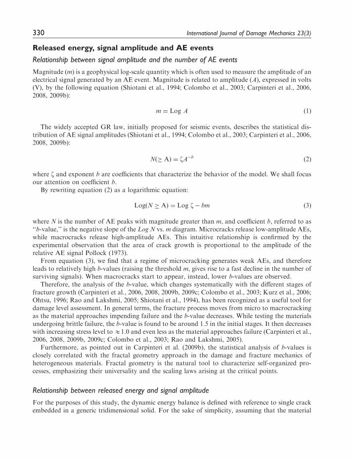
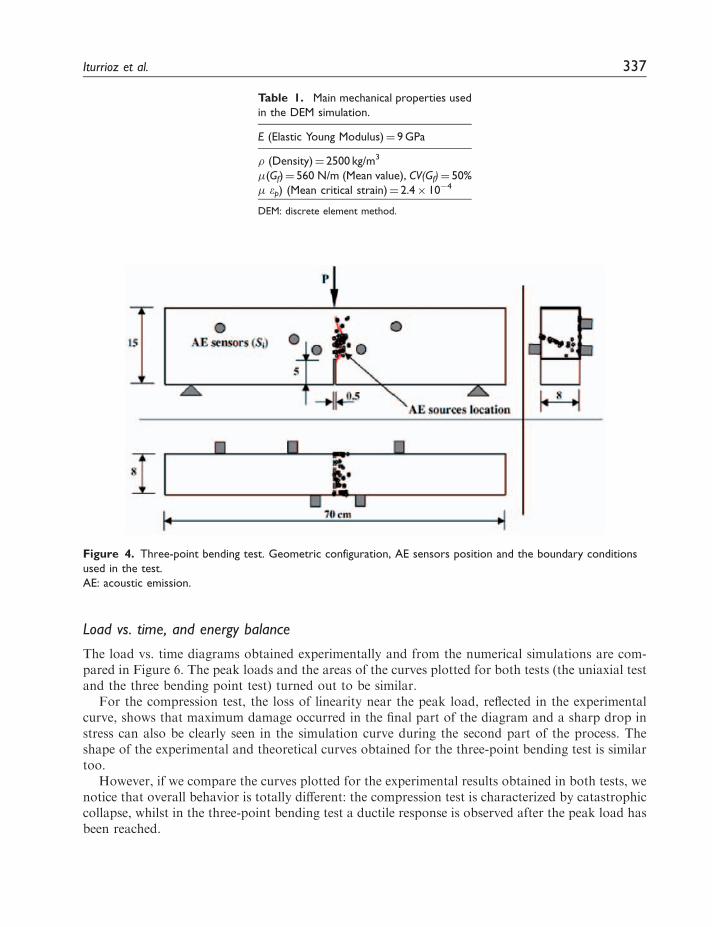
A concrete specimen in compression was investigated through AE monitoring in a laboratory test.Six AE transducers (denoted by SAE 1 to SAE 6) were applied to the surface of the specimen, a prismmeasuring 160� 160� 500mm3 (see Figure 1) Carpinteri et al. (2009b).
The test was performed under displacement control using an electronically controlled servo-hydraulic material testing system (MTS 311,31 model) with a capacity of 1800 kN, by imposing aconstant rate of displacement on the upper loading platen: the displacement rate was d�/dt¼ 10�5mm/s during the first 104 seconds and after that it was increased to 10�4mm/s up to failure.
This kind of machine is controlled by an electronic closed-loop servo-hydraulic system(Figure 2(b)). It is therefore possible to perform tests under load or displacement control.Displacement values are recorded by means of four strain gauges (HBM 1-LY41-50/120 model)placed on the specimen surface. In spite of the low value chosen for the displacement rate, thespecimen failed in a brittle manner, as can be seen in the load vs. time (strain) diagram in Figure 2(a),where the linear branch is seen to extend almost throughout the entire duration of the test.
Iturrioz et al. 333
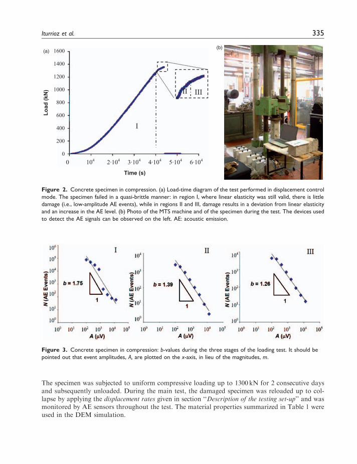
The characterization of the fracture process was carried out using the b-value analysis. Theloading test was divided into three stages: a first stage, where linear elasticity was still valid, andtwo subsequent stages characterised by deviations from linear elasticity and the existence of damage.The b-value calculated at the earliest stage of the loading test, where linear elasticity was still valid,was 1.75, an index reflecting a low damage level. The b-values calculated in the two following stagesof the damage region were 1.39 and 1.26, respectively, confirming the decreasing trend of the b-valueas the damage grows (Figure 3). The final configuration of the specimen after testing is shown inFigure 8.
Description of the numerical model
The numerical model of the specimen was made from 27� 27� 86 cubic modules. Each cubicmodule has a side length of L¼ 6mm, and hence the model contains 13� 104 nodes and 88� 104
elemental bars. Using the load vs. time diagram, and the information described in section‘‘Description of the testing set-up,’’ an initial elastic modulus of E¼ 9GPa was obtained. Thisvalue of E is lower than the classical value for concrete (normally 35�40GPa). This is due to thefact that the specimen had been subjected to a pre-damage process prior to conducting the main test.
Figure 1. Concrete specimen in compression. (a) Cross-section of the specimen. (b) Axonometric projection
showing the arrangement of the AE sensors. (c) Front views of the four specimen faces.
AE: acoustic emission.
334 International Journal of Damage Mechanics 23(3)
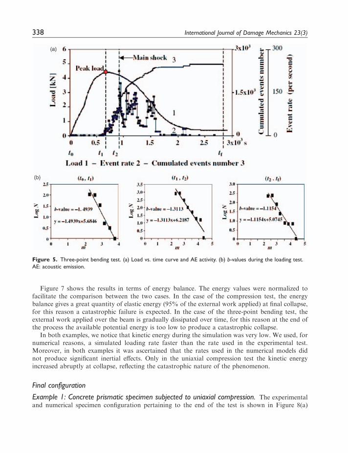
The specimen was subjected to uniform compressive loading up to 1300 kN for 2 consecutive daysand subsequently unloaded. During the main test, the damaged specimen was reloaded up to col-lapse by applying the displacement rates given in section ‘‘Description of the testing set-up’’ and wasmonitored by AE sensors throughout the test. The material properties summarized in Table 1 wereused in the DEM simulation.
(b)(a)
I
II III
0 104 2·104 3·104 4·104 5·104 6·104
Time (s)
1600
1400
1200
1000
800
600
400
200
0
Load
(kN
)
Figure 2. Concrete specimen in compression. (a) Load-time diagram of the test performed in displacement control
mode. The specimen failed in a quasi-brittle manner: in region I, where linear elasticity was still valid, there is little
damage (i.e., low-amplitude AE events), while in regions II and III, damage results in a deviation from linear elasticity
and an increase in the AE level. (b) Photo of the MTS machine and of the specimen during the test. The devices used
to detect the AE signals can be observed on the left. AE: acoustic emission.
Figure 3. Concrete specimen in compression: b-values during the three stages of the loading test. It should be
pointed out that event amplitudes, A, are plotted on the x-axis, in lieu of the magnitudes, m.
Iturrioz et al. 335
Model configuration and applied boundary conditions are shown in Figure 8(d). Parameter Gf isdefined as a random field with the mean value and the variation coefficient given in Table 1, using aprobability Weibull density distribution, and a correlation length equal to the level of discretization(L¼ 6mm).
A virtual sensor was placed in the position shown in Figure 1 (SAE 1). The acceleration perpen-dicular to the sensor surface was captured by the same virtual sensor and interpreted as a measure ofthe AE signals.
Example 2: Three-point bending test
Description of the testing set-up
In this example, a specimen was subjected to a three-point bending test and the AEs generated bygrowing microcracks were monitored. The specimen was a prism measuring 8� 15� 70 cm, with acentral 5-cm notch cut into it beforehand to produce a central crack, and with a fiber content of40 kg/m3 resulting in a Young’s modulus of 35GPa. The test was performed under displacementcontrol by imposing a constant displacement rate of 103mm/s.
Five AE transducers were secured to the specimen at the points shown in Figure 4(a). The load vs.time curve obtained for the specimen, with its softening branch characterizing the AE activity, isshown in Figure 5(a).
In order to investigate the behavior of the specimen by means of the b-value analysis, the load vs.time diagram was broken down into three stages: a first stage [t0,t1] extending from the initial time topeak load, a second stage [t1,t2] going from peak load to the peak of AE activity, or mainshock, anda third stage [t2,tp] going from the mainshock to the end of the process.
The b-values are shown for each stage in Figure 5(b): the values exhibited a decreasing trend,ranging from 1.49 to 1.11, as the specimen approached failure. The minimum value was obtained inthe softening branch of the load vs. time curve, and it became very close to the lower limit of 1theoretically predicted by Carpinteri et al. (1994, 2006, 2008, 2009c), as confirmed by the b-valuesobserved in most of specimens tested up to the failure.
Description of the numerical model
The numerical model was made from 140� 16� 30 cubic modules. Each cubic module has a sidelength of L¼ 5mm, and therefore the model contains 14� 104 nodes and 95� 104 elemental bars.Using the load vs. time diagram shown in the Figure 5(a), and the information given in section‘‘Description of the testing set-up,’’ we obtained E¼ 35GPa. The other parameters adopted aresummarized in Table 2.
Boundary conditions are shown in Figure 4(a). The excitation was applied to the model byintroducing a predetermined displacement at a velocity that did not give rise to significant inertialeffects in the model. The pre-crack was simulated so as to attenuate the strength of the bar in the pre-cracked zone.
Numerical results and comparison with the test results
Below are the numerical results obtained from the lattice model calculations and their comparisonwith the experimental values. The results obtained for the two cases described above are shown sideby side, whenever feasible, to facilitate their evaluation.
336 International Journal of Damage Mechanics 23(3)
Load vs. time, and energy balance
The load vs. time diagrams obtained experimentally and from the numerical simulations are com-pared in Figure 6. The peak loads and the areas of the curves plotted for both tests (the uniaxial testand the three bending point test) turned out to be similar.
For the compression test, the loss of linearity near the peak load, reflected in the experimentalcurve, shows that maximum damage occurred in the final part of the diagram and a sharp drop instress can also be clearly seen in the simulation curve during the second part of the process. Theshape of the experimental and theoretical curves obtained for the three-point bending test is similartoo.
However, if we compare the curves plotted for the experimental results obtained in both tests, wenotice that overall behavior is totally different: the compression test is characterized by catastrophiccollapse, whilst in the three-point bending test a ductile response is observed after the peak load hasbeen reached.
Figure 4. Three-point bending test. Geometric configuration, AE sensors position and the boundary conditions
used in the test.
AE: acoustic emission.
Table 1. Main mechanical properties used
in the DEM simulation.
E (Elastic Young Modulus)¼ 9 GPa
� (Density)¼ 2500 kg/m3
(Gf)¼ 560 N/m (Mean value), CV(Gf)¼ 50%
ep) (Mean critical strain)¼ 2.4� 10�4
DEM: discrete element method.
Iturrioz et al. 337
Figure 7 shows the results in terms of energy balance. The energy values were normalized tofacilitate the comparison between the two cases. In the case of the compression test, the energybalance gives a great quantity of elastic energy (95% of the external work applied) at final collapse,for this reason a catastrophic failure is expected. In the case of the three-point bending test, theexternal work applied over the beam is gradually dissipated over time, for this reason at the end ofthe process the available potential energy is too low to produce a catastrophic collapse.
In both examples, we notice that kinetic energy during the simulation was very low. We used, fornumerical reasons, a simulated loading rate faster than the rate used in the experimental test.Moreover, in both examples it was ascertained that the rates used in the numerical models didnot produce significant inertial effects. Only in the uniaxial compression test the kinetic energyincreased abruptly at collapse, reflecting the catastrophic nature of the phenomenon.
Final configuration
Example 1: Concrete prismatic specimen subjected to uniaxial compression. The experimentaland numerical specimen configuration pertaining to the end of the test is shown in Figure 8(a)
Figure 5. Three-point bending test. (a) Load vs. time curve and AE activity. (b) b-values during the loading test.
AE: acoustic emission.
338 International Journal of Damage Mechanics 23(3)
and (b), respectively. In these charts it is possible to appreciate that the upper sections of thespecimen are the most damaged and that cone-shaped ruptures have occurred near the specimenends. This is due to the confinement of transverse displacements at both ends (see Figure 8(d)).
In a configuration close to collapse, the transverse strain map shows (light grey portions inFigure 8(c)) the most badly damaged regions of the specimen subjected to high strains. From thisfigure it is also possible to understand how the main fracture mechanism occurs when ultimatestrength is reached with the transverse bars (perpendicular to the direction of loading) subjectedto tension.
Example 2: Three-point bending test. Two photographs of the beam in its final configuration anda detail of the DEM final configuration are given in Figure 9. In the DEM model, the fractured barsare denoted in dark grey, while light grey denotes bars only partially damaged. Undamaged barshave been omitted to improve the visualization.
In Figure 9(d) and (e), two lateral views of the damage configuration are shown, one at t¼ 1200 s(close to the peak load) and the other at t¼ 2800 s (close to the final collapse). The general config-urations obtained from the numerical and experimental results are similar.
Figure 6. Load vs. time, comparison between experimental results (continuous line) and numerical simulation
In Figure 10(a) and (b), the transverse sections of the beam in x¼L/2, at t¼ 1200 s and t¼ 2800 s,show the bars damaged and fractured during the loading process. In Figure 10(c), we see a detail ofthe lateral view close to the central crack. The information shown in these pictures could be used tocompute the fractal dimension of the fractured area, and this issue will be addressed in a futurework.
Figure 8. (a) Experimental rupture configuration. (b) Numerical rupture configuration, plotting of the nodes.
(c) Map of damage (severe damage is denoted in light grey). (d) Initial configuration in which the applied boundary
conditions are shown.
Figure 7. Normalized energy balance vs. time (Eele: elastic energy, Ek: kinetic energy, Ed: dissipated energy; Emax
EeleþEkþEd at tmax). (a) Uniaxial compression test (Emax¼ 4888 Nm). (b) Three-point bending test (Emax¼ 0.65 Nm).
340 International Journal of Damage Mechanics 23(3)
AE and N vs. time, b-value analysis
The AE event amplitudes vs. time charts obtained by DEM simulations are shown for both exam-ples (Figure 11(a) and (b)). In these figures, the coordinate scales are normalized to facilitate thecomparison between the two examples. The load variation obtained in the numerical simulation isplotted in light grey.
In Figure 12(a) and (b), the results are shown in terms of cumulated number of AE events, N, andAE event rate, Ninst, vs. time. In this figure too, the load vs. time curve is shown in light grey.
Finally, in Figure 13(a) and (b), the curves that link the cumulated number of AE event and theirmagnitudes are presented in logarithm scale. By using these curves it is possible to compute theb-value for each selected time-period.
To represent these diagrams, relative signal amplitudes were computed (we defined A¼ h/ho,where ho¼ 100mm/s2). Then, only signals of amplitudes greater than the predetermined thresholdwere taken into account. We set a fixed threshold Athres¼ h/ho¼ 30,000 for the first example andAthres¼ h/ho¼ 1500 for the second. For this reason, the number of events analyzed in the simulationswas limited (fewer than 200 in each example).
In general, to carry out a consistent analysis from a statistical point of view we need as a min-imum a thousand events per example. By applying a lower imposed displacement rate and consider-ing a lower value for the fixed threshold, Athres, it would be possible to identify more AE peaks.However, in order to increase the number of events by considering A>Athres, it would be necessaryto increase the discretization level. For this reason, the simulations performed should be regarded aspreliminary, nevertheless they are useful to capture the general trends.
Figure 9. (a) and (b) Details of the final experimental configuration. (c) Detail of the final numerical configuration.
(d) Lateral view of the damage configuration at t¼ 1200 s. (e) Lateral view of the damage configuration at t¼ 2800 s.
In the numerical configuration obtained by DEM simulations, the bars that have exhausted their strength are shown in
dark grey, while light grey denotes the bars only partially damaged. Undamaged bars are omitted to improve the
visualization. DEM: discrete element method.
Iturrioz et al. 341
(a) (t=1200s) (b) (c)
(a) (t=2800s) (b) (c)
z
y
z
x
Figure 10. (a) Central crack for x¼ L/2, only the fractured and damaged bars are shown. (b) Central crack for x¼ L/
2, only the fractured bars are shown. (c) Detail of the side view of the beam with only the fractured bars shown. The
three figures at the top were plotted at t¼ 1200 s, the three figures below were plotted at t¼ 2800 s. The bars that
have exhausted their strength are denoted in dark grey, while light grey indicates bars only partially damaged.
Undamaged bars have been omitted to improve the visualization.
342 International Journal of Damage Mechanics 23(3)
Figure 12. Cumulated number of AE events, N, AE events rate, Ninst, and load vs. time diagrams. (a) Uniaxial test.
(b) Three-point bending test.
AE: acoustic emission.
Figure 11. Load vs. time (continuous line) and AE events amplitude vs. time (vertical bars). Both coordinate axes
were normalized to the maximum value. (a) Uniaxial test. (b) Three-point bending test.
Iturrioz et al. 343
By comparing the two examples we find that:
(i) AE event amplitudes in the uniaxial compression test are shown in Figure 11(a). Event amp-litude is seen to increase smoothly throughout the loading process up to the catastrophiccollapse, which is characterized by the highest amplitude AE event, labeled (a1) in thisfigure. The amplitude of this last AE event is four times as high as the amplitude of the AEpeak event that occurs immediately before specimen collapse, and is labeled (a2) in the figure.
(ii) AE event amplitudes in the three-point bending test are shown in Figure 11(b). In this case,mechanical behavior is completely different than in the first test: here a high-amplitude event(labeled (b1) in the figure) occurs at the beginning of the process. This AE peak event occursdue to a premature advance of the existing macro-crack. A second high-amplitude event,labeled (b2), appears in the proximity of the maximum load. After this characteristic event,the other events are of lesser amplitude and maintain the same level until the end of the test.
(iii) The clearly different behavior observed in the uniaxial test for cumulated AE events, N, andAE rate, Ninst, makes it possible to define two time intervals for the analysis of the b-value: [0,18000] s and [18000, tf] s, where tf is the time of the final collapse. The dashed vertical line inFigure 12(a) indicates the point of separation between these two intervals.
(iv) The cumulated AE events, N, and AE rate, Ninst, curves obtained from the three-point bendingtest are shown in Figure 12(b). In this case, two time intervals for the b-value analysis are alsodefined: [0, 1200] s and [1200, tf] s. The dashed vertical line in Figure 12(b) indicates the pointof separation between these two intervals.
(v) By comparing Figure 12(b) with Figure 5(a), showing the experimental results, we notice thatin the latter AE events do not occur until peak load, then a concentration of events emerges inthe post-peak region; finally the number of AE events abruptly decreases. This last behavior isevidenced in the numerical simulation.
However, the main differences between experimental and numerical results are concentrated atthe beginning of the two diagrams, where, in the experimental case, very few events are detected untilthe peak load is reached and, in the numerical simulation, great AE activity is observed. Thisdiscrepancy could be justified by the mechanical properties adopted in the DEM simulation, i.e.the same distribution for all the elements (see Table 2); in this manner, the stress concentration at the
b[0,18000]= 1.47
b[18000,tf]= 1.16
0
0.5
1
1.5(a) (b)
4.0 4.5 5.0 5.5 6.0
m
Log(
Nac
um)
b[0,1200] =1.10
b[1200,tf]= 1.03
0
0.4
0.8
1.2
1.6
2
3 3.4 3.8 4.2 4.6m
Log
(Nac
um)
Figure 13. b-values obtained from the numerical simulation of the damage process. (a) Uniaxial test.
(b) Three-point bending test.
344 International Journal of Damage Mechanics 23(3)
tip of the pre-existing crack shows, as it should, an intense AE activity at the beginning ofthe loading process, while in the real specimen the local mechanical properties may be lower inthe vicinity of the pre-existing crack (damaged region near the crack tip produced during specimenmanufacture) than in the rest of the specimen. This event, especially at the beginning of the loadingprocess, may have given rise to a lower AE activity.
(vi) The b-values obtained in the two time intervals defined for the compression test are shown inFigure 13(a). The b-values obtained in the numerical simulation show a decreasing trendduring the evolution of the damage process and are compatible with the experimentalvalues. Moreover, the numerical b-values fall between the limits [1.5,1] indicated byCarpinteri et al. (2009a). In this case, we have b¼ 1.47 for the first interval and b¼ 1.16 forthe second, this means that the damage process is characterized by a progressive localizationidentified through the fractal dimension 2b¼D of the damage domain.
(vii) The b-values obtained in the two time intervals defined for the three-bending point test are shownin Figure 13(b). In this case, the b-values are close to 1.0 from the start of the process. This meansthat the propagating crack is close to a preferential surface throughout the test duration.
AE events and energy parameters
The relationship between the energy released during the fracture process, Es, and signal amplitude,A, is analyzed. Considering Chakrabarti and Benguigui (1997), Es is linked with the drops in poten-tial energy taking place during the damage process. With the aim of capturing the energy released,Es, in the DEM context, we propose to compute the increments in kinetic energy between twosuccessive integration times, using the following expression:
�Ek tið Þ ¼ Ek tið Þ � Ek ti�1ð Þ ð17Þ
where Ek is the kinetic energy in the discretized time during the simulation.Using the equation (6) and the discussion carried out by Scholz (2002), briefly commented in the
section ‘‘Relationship between released energy and signal amplitude,’’ we can assume the validity ofthe following relationship:
�EkðtFaÞ
�EkkðtFbÞ¼
EsðtFaÞ
EsðtFbÞð18Þ
where tFa and tFb are the times at which the potential energy drops during the simulation.In this way, equation (8) can be written in terms of DEk:
Log �EkðtFÞð Þ ¼ Log þ cEkLog AðtFÞ ð19Þ
where is a coefficient, and cEk is an estimate of the c coefficient in the Richter law presented inequations (7) and (8).
In a similar way, we propose rewriting equation (13), which links the number of events N (�Es) toreleased energy Es. Using increments DEk we can write:
LogN 4 ¼ �EkðtFÞð Þ ¼ Log � þ dEk Log�EkðtFÞ ð20Þ
where � is a coefficient and dEk is an estimate of the d coefficient in equation (13).
Iturrioz et al. 345
The variations taking place during the damage process in elastic (or potential) kinetic energy anddissipated energy are illustrated in Figure 7(a) and (b).
It is also possible to compute the increments in dissipated energy between two successive inte-gration times using the following expression:
�Ed tið Þ ¼ Ed tið Þ � Ed ti�1ð Þ ð21Þ
In Figure 14(a), the increments in dissipated energy, DEd, are plotted, and Figure 14(b) shows thevariations in DEk determined from equation (17). In these figures, time tF is the time when the dropin potential energy typically occurred during the simulation process.
A typical AE event is superposed with the DEd and DEk increments during the simulation processin Figure 15(a). A zoom of the beginning of this AE event is shown in Figure 15(b), where it can beclearly seen that the AE signal undergoes a certain delay in time with respect to the DEk and DEd
increments. This is due to the fact that when a localized fracture occurs in the specimen, the energyvalues are immediately computed, while the mechanical waves, which spread due to localized frac-ture in the specimen, need some additional time to reach the AE sensor.
Notice that when a drop in potential energy occurs, part of this potential energy is dissipated andpart becomes kinetic energy. In Figure 16, the increments in elastic, dissipated and kinetic energy inthe vicinity of a typical AE event illustrate the complex interaction between these quantities.
Finally, Figure 17(a) and (b) show the cumulative distributions in equation (20) represented in abi-logarithmic scale. For both examples, the same intervals used in the b-values computationwere used. The b, c and d coefficients computed by means of the numerical simulation are summar-ized in Table 3.
From Table 3 we can see that:
(i) The c¼ b/d ratios are close to the theoretical value 1.5 indicated by Richter (1958) as describedin section ‘‘Released energy, signal amplitude and AE events.’’
Figure 14. (a) Variations of dissipated energy increments Ed, dissipated energy Ed and elastic energy Eele during the
entire simulation process. (b) Variations of kinetic energy increment Ek and kinetic energy Ek during the entire
simulation process.
346 International Journal of Damage Mechanics 23(3)
(ii) From the evaluation of released energy, it is possible to say that coefficients d are also sensitiveto the evolution of damage, and hence d-values decrease with increasing damage and cracklocalization.
(iii) From the Table it is also evident that coefficient c increases with damage, but its value does notexceed the limit of 2.
Relationship between Es, N and A and time
Below, we extend the idea expressed in Carpinteri et al. (2007) where AE results are expressed interms of an accumulated parameter (N, A or a measure of Es) normalized to its maximum value vs.
Figure 16. Increments in elastic energy (dark grey line), kinetic energy (black line) and dissipated energy (light grey
line) vs. time in the vicinity of a typical AE event. The units on the vertical axis are arbitrary.
AE: acoustic emission.
Figure 15. (a) The three types of signals overlapped. Signal amplitudes were modified to be able to put them in the
same scheme. (b) Details of the beginning of the peak event. Increment in dissipated energy Ed(t), increment in kinetic
energy Ek (t) and the AE signal produced. AE: acoustic emission.
Iturrioz et al. 347
(t/tmax). The behaviors of these functions give us useful information about the specimen damagetime-scaling.
We propose here the following relations:
Nacum
Nacumð Þmax
/t
tmax
� ��Nð22Þ
Aacum
Aacumð Þmax
/t
tmax
� ��Að23Þ
�Ek acum
�Ek acumð Þmax
/t
tmax
� ��Kð24Þ
In the previous equations, Nacum/(Nacum)max is the number of cumulated AE events normalized totheir maximum value; Aacum/(Aacum)max the normalized number of cumulated AE signals ampli-tudes and DEk_acum/(DEk_acum)max the normalized number of cumulated kinetic energy incrementsrelated to the AE events. All the expressions are related to normalized time t/tmax.
These relationships are illustrated in bi-logarithmic scale in Figures 18(a) and 19(b) for the uni-axial compression test and the three-points bending test, respectively. In this way, the values ofcoefficients �N, �A and �K are obtained. The same relationships are plotted on a linear scale in
d[18000,tf] = 0.59
d[0,18000]= 0.96
0
0.4
0.8
1.2
1.6
2(a) (b)
2 2.8 3.6 4.4 5.2
log Ek
Log
(Nac
um)
d[1200,tf]= 0.64
d[0,1200] = 0.750
0
0.4
0.8
1.2
1.6
2
2.4 2.8 3.2 3.6 4Log Ek
Log
(Nac
um)
Figure 17. The d coefficients obtained in (a) uniaxial test and (b) three-point bending test.
Table 3. b, d and c¼ b/d coefficients for the two specimens analyzed.
Compression test Bending test
[0,18000]s [18000,tf]s [0,1200]s [1200,tf]s
b¼ 1.47 b¼ 1.16 b¼ 1.1 b¼ 1.01
d¼ 0.96 d¼ 0.59 d¼ 0.75 d¼ 0.64
c¼ 1.53 c¼ 1.97 c¼ 1.47 c¼ 1.58
348 International Journal of Damage Mechanics 23(3)
Figures 18(b) and 19(b). Finally, the values of the � coefficients computed for both tests are sum-marized in Table 4.
It should be noted that only values greater than t/tmax¼ 0.4 were used to perform the regression inthe bi-logarithmic diagrams. In Carpinteri et al. (2007) this point was discussed. The authorsjustified using only this part of the process because in the first part, t/tmax[0, 0.4], the resultscould be highly influenced by the specific boundary conditions of the tests.
By analyzing the results presented in Figures 18, 19 and in Table 4, we find that the � coefficientsgive us useful information about the last part of the damage process.
Specifically, we observe that:
(i) �N¼ 0.98 indicates that in the compression test the AE events number grows at a constant ratethroughout the loading process. The same information appears in the linear branch of theNacum vs. time curve, shown in Figure 18(b). On the other hand, AE events amplitudes increaseby a factor of �A¼ 2.02, while the cumulated number of kinetic energy increments, corres-ponding to each AE event, increases by a higher factor: �K¼ 3.2.
(ii) Coefficients �N and �A have virtually the same values in the three-points bending test. Thevalues of these coefficients indicate that not only the AE events number but also event amp-litudes have a tendency to diminish as the damage process advances. The relationship betweenthe kinetic energy and the damage process is characterized by the coefficient �K¼ 1.36, whichimplies a smoother increase than in the compression test example.
(iii) If we compare the � coefficients of the two examples, we find that the larger values recordedfor the compression test characterize a catastrophic collapse. This information is not includedin the b-values analysis that measures the damage localization process throughout the testsduration.
AE event frequency variations during the damage process
In this section, the simulation results are analyzed in terms of AE signal frequency variations. InSchiavi et al. (2011), in which a test similar to the one analyzed in this paper was discussed, AEfrequency variation was proposed as a parameter to evaluate the damage process. The resultsobtained in the numerical simulations of both tests are given in Figures 20 and 21.
Some remarks on the results are shown above in Figures 20 and 21:
(i) The frequency spectrums of the AE events that occur during the damage processes in both testsare shown in Figures 20(a) and 21(a). As regards the uniaxial compression test, the energyspectrum is close to 70 kHz at the beginning of the test, while it shifts to 120 kHz at the end ofthe process (see Figure 20(a)). Moreover, signal energy distribution is broader in the final stageof the damage process. The same tendency was observed in Schiavi et al. (2011). In the three-point bending test, the shape of the spectrum does not show a clear tendency to change duringthe damage process (see Figure 21(a)).
(ii) The highest peak frequencies (see (VII) in Figures 20(a) and 21(a)) are correlated with thediscretization level. Remembering that L stands for the elemental cube side, E is Young’smodulus and � material density, it is possible to compute the p-wave velocity in each baras c� ¼ (E/�)0�5. On the other hand, the natural vibration frequency of vibration of the normalbars of the lattice model is fc¼ 1/Tc, where Tc¼ 2�L/c�. By substituting the parameters cor-responding to both examples, we obtain: for the uniaxial compression test fc¼ 160 kHz, and for
Iturrioz et al. 349
the three-point bending test fc¼ 374 kHz. Peaks around these frequencies appear in Figures 20and 21 and are marked with a label (VII).
(iii) The evolution during the damage process of the two lower peak frequencies, f1 and f2, and themaximum peak frequency, fp, is shown for both examples in Figures 20(b) and 21(b). Time andfrequency values are normalized to facilitate the comparison. The f1, f2 and fp frequencies are
-1.6
-1.4
-1.2
-1
-0.8
-0.6
-0.4
-0.2
0-0.6 -0.5 -0.4 -0.3 -0.2 -0.1 0
Log(t/tmax)(a)
(b)
Log(
X/X
max
)
0
0.2
0.4
0.6
0.8
1
0 0.2 0.4 0.6 0.8 1
t/tmax
X/X
max
98.0
maxmax
)()( t
t
N
N
acum
acum ∝
02.2
maxmax
)()( t
t
A
A
acum
acum ∝
2.3
maxmax_
_ )()( t
t
E
E
acumk
acumk ∝Δ
Δ
)(Log98.0)(
Logmaxmax t
t
N
N
acum
acum ∝
R2=0.97
)(Log02.2)(
Logmaxmax t
t
A
A
acum
acum ∝
R2=0.99
)(Log20.3)(
Logmaxmax_
_
t
t
E
E
acumk
acumk ∝Δ
Δ
R2=0.99
Figure 18. Nacum/(Nacum)max, Aacum/(Aacum)max and (Ek_acum)/(Ek_acum)max vs. t/tmax diagrams obtained from the com-
pression test. (a) Bi-logarithm scale. (b) Linear scale. The R value measures the linear correlation of these adjustments.
350 International Journal of Damage Mechanics 23(3)
-0.6
-0.5
-0.4
-0.3
-0.2
-0.1
0-0.5 -0.4 -0.3 -0.2 -0.1 0
Log(t/tmax)
Log(
X/X
max
)0
0.2
0.4
0.6
0.8
1
0 0.2 0.4 0.6 0.8 1
t/tmax
X/X
max
)(Log59.0)(
Logmaxmax t
t
N
N
acum
acum ∝
R2=0.96
)(Log60.0)(
Logmaxmax t
t
A
A
acum
acum ∝
R2=0.98
)(Log36.1)(
Logmaxmax_
_
t
t
E
E
acumk
acumk ∝Δ
Δ
R2=0.99
59.0
maxmax
)()( t
t
N
N
acum
acum ∝
60.0
maxmax
)()( t
t
A
A
acum
acum ∝
36.1
maxmax_
_ )()( t
t
E
E
acumk
acumk ∝Δ
Δ
(a)
(b)
Figure 19. Nacum/(Nacum)max, Aacum/(Aacum)max and (Ek_acum)/(Ek_acum)max vs. t/tmax diagrams obtained from the bending
test. (a) Bi-logarithm scale. (b) Linear scale.
Table 4. � coefficients for the two specimens analyzed.
�N �A �K
Compr. test 0.98 2.02 3.2
Bending test 0.59 0.6 1.36
Iturrioz et al. 351
also marked with small circles in the spectrums shown in Figures 20(a) and 21(a), and markedwith labels (I) to (VI). In the uniaxial compression test, Figures 20 and 21(b) show a cleartendency of the f1 and f2 peak frequencies to decrease with increasing damage growth. Thesame tendency was also observed by Schiavi et al. (2011). The values of the highest frequenciesfp does not change significantly during the damage process. Only at the final collapse theirvalues change abruptly. Moreover, in the case of the three-point bending test, the peakfrequencies, f1 f2 and fp, do not show a clear tendency to decrease during the damage process(see Figure 20(b)).
0.0
0.2
0.4
0.6
0.8
1.0
1.2
0.0 0.2 0.4 0.6 0.8 1.0t/tmax
f/fm
ax
f1/f1max
f2/f2max
fp/fpmax
(VII)
(III)
(I) (II)(IV)
(V)
(VI)
t/tmax =0.08t/tmax =1
f[kHz]
(a)
(b)
Figure 20. Frequency variations during the damage process in the compression test. (a) Two frequency spectrums
were computed, at the beginning and at the end of the damage process. (b) Variations of the first (f1), second (f2) and
maximum peak (fp) frequencies during the damage process (in each case time and frequencies were normalized to the
maximum value).
352 International Journal of Damage Mechanics 23(3)
Finally, the AE events vs. time diagrams obtained experimentally and numerically in the three-point bending test are shown in Figure 22. Notice that the time duration of the AE events is similar.In Figure 23, the AE events spectrums are compared and it can be seen that the numerical resultspresent a wider spectrum. The maximum peak frequencies of the signals obtained experimentallyand numerically do not match. However, for other AE events, the maximum peak values obtainednumerically were in close agreement with the experimental ones.
0.0
0.2
0.4
0.6
0.8
1.0
1.2
(a)
(b)
0.0 0.2 0.4 0.6 0.8 1.0t/tmax
f/fm
ax
f1/f1max
f2/f2max
fp/fpmax
t/tmax=0.09 t/tmax=1
(I)
(II)
(III)
(IV)
(V)
(VI)
(VII)
f[kHz]
Figure 21. Frequency variations during the damage process in the three-point bending test. (a) Two frequency
spectrums were computed, at the beginning and at the end of the damage process. (b) Variations of the first (f1),
second (f2) and maximum peak (fp) frequencies during the damage process (in each case time and frequencies were
normalized to the maximum value).
Iturrioz et al. 353
Conclusions
In this work, two experimental tests carried out on concrete specimens loaded up to failure areanalyzed. One was a prismatic specimen subjected to uniaxial compressive loading, the other was apre-cracked beam subjected to the three-point bending test. For both examples, experimental andnumerical results are presented. The numerical simulations were performed using a version of thetruss-like DEM. During the tests, the AE technique was used to monitor the damage process takingplace in the specimens. The numerical and experimental results obtained in the two examples arecompared, and their intrinsic differences are identified.
Figure 23. Comparison between the experimental and numerical spectrums obtained in the three-point bending
test for a typical AE event.
AE: acoustic emission.
Figure 22. Typical AE signal vs. time diagrams. (a) Experimental signal. (b) Numerical signal from the three-point
bending test example.
AE: acoustic emission.
354 International Journal of Damage Mechanics 23(3)
From these analyses, the following conclusions may be drawn.
– The comparison between the experimental and numerical results shows reasonable correlations,for both examples, in terms of conventional results, such as load vs. time and final configurations.
– In terms of the distribution of AE event amplitudes in time, the results were seen to be consistent,and any differences observed between the experimental and numerical results were accounted for.It is important to point out that the numerical b-values obtained are compatible with the experi-mental values and in good agreement with damage theories (Carpinteri et al., 2009b), showing atendency to decrease during the damage process.
– The low number of AE events analyzed in the numerical simulations (fewer than 200 events inboth cases) compared with the number determined by AE monitoring is an issue to be discussedin detail in relation to the results obtained. However, the aim of these numerical simulations, asmentioned above, was to identify the general trends on a preliminary base. To increase thenumber of AE events analyzed in the numerical simulations you need a finer discretization,something we shall do after this initial exploration of the applicability of DEM simulations tothis kind of process.
– Using the AE data calculated by the numerical models, the results in terms of released energy arevery useful to gain a better understanding of damage evolution of each example analyzed. Thecorrelations between the b-values and the analogous d-values, which describe the scaling ofreleased energy in terms of DEk increments, are shown according to the fundamental law pro-posed by Richter (1958). On the basis of this evaluation, the numerical d-values, as well as theb-values, appear sensitive to the evolution of damage: they decrease with increasing damage andcrack localization.
– The variations in time of the cumulated AE events number, AE amplitudes and cumulatedincrements in kinetic energy were computed, by means of the � coefficients, using the numericalmodels of both examples. The � coefficients made it possible to compare damage evolution ineach example, showing that they are precursors of the final modalities of structural collapse.
– The numerical results obtained for the AE signal frequencies in the uniaxial compression testshow variations that are consistent with the experimental data obtained by Schiavi et al. (2011).In the three-point bending test, no substantial changes in AE peak frequencies were observedinstead. For this reason, it may be concluded that the clear tendency exhibited by peak frequen-cies to decrease during the damage process indicates that a catastrophic collapse is taking place inthe specimen subjected to uniaxial compression.
– This study has shown the potential applications of the truss-like DEM not only to simulate AEmonitoring analysis but also to provide a better understanding of the relationships between thebasic AE parameters.
– Finally, in the application of the AE technique and the numerical approach here presented, specialattention will be taken in future research to study the damage evolution in fiber-reinforced quasi-brittle materials. Three new references by Tarantino (2013) and by Nobili et al. (2012, 2013) will betaken into account for this approach: the first one about the aspects related to damage and theremaining ones with regard to the applications of the AE technique to fiber-reinforced concrete.
Acknowledgements
The financial support provided by the Regione Piemonte (Italy) through the RE-FRESCOS Project is gratefullyacknowledged. The authors also thank the Brazilian agency CNPq – National Council for Scientific andTechnological Development for funding this research.
Iturrioz et al. 355
References
Aki K (1967) Scaling law of seismic spectrum. Journal of Geophysical Research 72: 1217–1231.Aki K and Richards PG (2002) Quantitative Seismology, 2nd ed. University Sciences Books.
Brara A, Camborde F, Klepaczko JR, et al. (2001) Experimental and numerical study of concrete at high strain
rates in tension. Mechanics of Material 33: 33–45.
Carpinteri A (1994) Scaling laws and renormalization groups for strength and toughness of disordered mater-
ials. International Journal of Solids and Structures 31: 291–302.
Carpinteri A, Lacidogna G and Pugno N (2007) Structural damage diagnosis and life-time assessment by
Colombo S, Main IG and Forde MC (2003) Assessing damage of reinforced concrete beam using ‘‘b-value’’
analysis of acoustic emission signals. Journal of Materials in Civil Engineering 15: 280–286.Cundall PA and Hart RD (1989) Numerical modelling of discontinua. In: Proc 1st US Conference Discrete
Element Method, Golden, CO, 1-17.Dalguer LA, Irikura K and Riera JD (2003) Simulation of tensile crack generation by three-dimensional
dynamic shear rupture propagation during an earthquake. Journal of Geophysical Research 108(B3): 2144.Dalguer LA, Irikura K, Riera JD, et al. (2001) The importance of the dynamic source effects on strong ground
motion during the 1999 Chi-Chi, Taiwan, earthquake: Brief interpretation of the damage distribution on
buildings. Bulletin of the Seismological Society of America 91: 1112–1127.
Hillerborg A (1971) A model for fracture analysis. Cod LUTVDG/TVBM 300: 51–81.Iturrioz I, Miguel LFF and Riera JD (2009) Dynamic fracture analysis of concrete or rock plates by means of
the Discrete Element Method. Latin American Journal of Solids and Structures 6: 229–245.Kanamori H and Anderson DL (1975) Theoretical basis of some empirical relations in seismology. Bulletin of
the Seismological Society of America 5: 1073–1095.Kosteski L, Barrios R and Iturrioz I (2008) Determinacion de Parametros Fractomecanicos Estaticos y
Dinamicos utilizando el Metodo de los Elementos Discretos compuestos por barras. Revista
Internacional Metodos Numericos para Calculo y Diseno en Ingenierıa. Cimne 24: 323–343.
Kosteski L, Barrios R and Iturrioz I (2009) Fractomechanics parameter calculus using the Discrete Element
Method. Latin American Journal of Solids and Structures 6: 301–321.
Kosteski LE, Barrios R and Iturrioz I (2012) Crack propagation in elastic solids using the truss-like discrete
element method. International Journal of Fracture 174: 139–161.
Kosteski L, Iturrioz I, Batista RG, et al. (2011) The truss-like discrete element method in fracture and damage
mechanics. Engineering Computations 6: 765–787.
Krajcinovic D (1996) Damage Mechanics. Elsevier, Amsterdam.Kurz JH, Finck F, Grosse CU, et al. (2006) Stress drop and stress redistribution in concrete quantified over
time by the b-value analysis. Structural Health Monitoring 5: 69–81.Lemaitre J and Chaboche JL (1990) Mechanics of Solid Materials. Cambridge: University Press.
356 International Journal of Damage Mechanics 23(3)
Lu C, Mai YW and Xie H (2005) A sudden drop of fractal dimension: a likely precursor of catastrophic failure
in disordered media. Philosophical Magazine Letters 85: 33–40.
Mastilovic S (2011a) Some observations regarding stochasticity of dynamic response of 2D disordered brittle
lattices. International Journal of Damage Mechanics 20: 245–265.
Mastilovic S (2011b) Further remarks on stochastic damage evolution of brittle solids under dynamic tensile
loading. International Journal of Damage Mechanics 20: 900–992.
Miguel LFF, Riera JD and Iturrioz I (2008) Influence of size on the constitutive equations of concrete or rock
dowels. International Journal for Numerical and Analytical Methods in Geomechanics 32: 1857–1188.
Miguel LFF, Iturrioz I and Riera JD (2010) Size effects and mesh independence in dynamic fracture analysis of
Munjiza A (2009) Special issue on the discrete element method: aspects of recent developments in computa-
tional mechanics of discontinua. Engineering Computations 26: 6.
Munjiza A, Bangash T and John NWM (2004) The combined finite-discrete element method for structural
failure and collapse. Engineering Fracture Mechanics 71: 469–483.
Nayfeh AH and Hefzy MS (1978) Continuum modeling of three-dimensional truss-like space structures. AIAA
Journal 8: 779–787.
Nobili A, Lanzoni L and Tarantino AM (2012) Performance evaluation of a polypropylene-based draw-wired
fibre for concrete structures. Construction and Building Materials 28: 798–806.
Nobili A, Lanzoni L and Tarantino AM (2013) Experimental investigation and monitoring of a Polypropylene-
based fiber reinforced concrete road pavement. Construction and Building Materials 38: 491–496.
Ohtsu M (1996) The history and development of acoustic emission in concrete engineering. Magazine of
Concrete Research 48: 321–330.
Pollock AA (1973) Acoustic emission-2: acoustic emission amplitudes. Non-Destruct Test 6: 264–269.Rabczuk T and Belytschko T (2004) Cracking particles: a simplified meshfree method for arbitrary evolving
cracks. International Journal for Numerical Methods in Engineering 61(13): 2316–2343.Rabczuk T and Belytschko T (2007) A three-dimensional large deformation meshfree method for arbitrary
evolving cracks. Computer Methods in Applied Mechanics and Engineering 196(29–30): 2777–2799.Rabczuk T, Bordas S and Zi G (2007) A three-dimensional meshfree method for continuous multiplecrack
initiation, nucleation and propagation in statics and dynamics. Computational Mechanics 40(3): 473–495.Rao MVMS and Lakshmi KJP (2005) Analysis of b-value and improved b-value of acoustic emissions accom-
panying rock fracture. Current Science 89: 1577–1582.Richter CF (1958) Elementary Seismology. San Francisco and London: W. H. Freeman.Riera JD (1984) Local effects in impact problems on concrete structures. In: Proceedings, conference on struc-
tural analysis and design of nuclear power plants, Porto Alegre, RS, Brazil, Vol. 3, CDU
264.04:621.311.2:621.039.Riera JD and Iturrioz I (1995) Discrete element dynamic response of elastoplastic shells subjected to impulsive
loading. Communications in Numerical Methods in Engineering 11: 417–426.Riera JD and Iturrioz I (1998) Discrete element model for evaluating impact and impulsive response of
reinforced concrete plates and shells subjected to impulsive loading. Nuclear Engineering and Design 179:
135–144.
Rinaldi A and Lai YC (2007) Statistical damage theoryof 2D lattices: Energetics and physical foundations of
damage parameter. International Journal of Plasticity 23: 1769–1825.
Rinaldi A, Krajcinovic D, Peralta P, et al. (2008) Lattice models of polycrystalline microstructures: A quan-
titative approach. Mechanics of Materials 40: 17–36.
Rios RD and Riera JD (2004) Size effects in the analysis of reinforced concrete structures. Engineering
Structures 26: 1115–1125.
Rundle J, Turcotte D, Shcherbakov R, et al. (2003) Statistical physics approach to understanding the multiscale
dynamics of earthquake fault systems. Reviews of Geophysics 4: 8755–81209.
Schiavi A, Nicolini G, Tarizzo P, et al. (2011) Acoustic emissions at high and low frequencies during compres-
sion tests in brittle materials. Strain 47(Suppl 2): 105–110.
Iturrioz et al. 357
Schnaid F, Spinelli L, Iturrioz I, et al. (2004) Fracture mechanics in ground improvement design. GroundImprovement 8: 7–15.
Scholz CH (1968) The frequency-magnitude relation of microfracturing in rock and its relation to earthquakes.Bulletin of the Seismological Society of America 58: 99–415.
Scholz CH (2002) The Mechanics of Earthquakes and Faulting, 2nd ed. New York, US: Cambridge UniversityPress.
Shiotani T, Fujii K, Aoki T, et al. (1994) Evaluation of progressive failure using AE sources and improved
b-value on slope model tests. Progress in Acoustic Emission 7: 529–534.Tarantino AM (2013) Equilibrium paths of a hyperelastic body under progressive damage. Journal of Elasticity.
DOI: 10.1007/s10659-013-9439-0.
Turcotte DL, Newman WI and Shcherbakov R (2003) Micro and macroscopic models of rock fracture.Geophysical Journal International 152: 718–728.
358 International Journal of Damage Mechanics 23(3)


![Engineering Failure Analysis - polito.it...The process is called by Munjiza [25] “Computational Mechanics of Discontinua” and it is now as an integral part of cutting-edge research](https://static.documents.pub/doc/80x56/5f79caf9310aeb01da0b065b/engineering-failure-analysis-the-process-is-called-by-munjiza-25-aoecomputational.jpg)


