Acoustic holography as a metrological tool for characterizingmedical ultrasound sources and fields

Oleg A. Sapozhnikov,a) Sergey A. Tsysar, and Vera A. Khokhlovaa)

Department of Acoustics, Physics Faculty, Moscow State University, Leninskie Gory, Moscow 119991, Russia

Wayne Kreiderb)

Center for Industrial and Medical Ultrasound, Applied Physics Laboratory, University of Washington,1013 Northeast 40th Street, Seattle, Washington 98105, USA

(Received 21 April 2015; revised 26 July 2015; accepted 30 July 2015; published online 16September 2015)

Acoustic holography is a powerful technique for characterizing ultrasound sources and the fields

they radiate, with the ability to quantify source vibrations and reduce the number of required

measurements. These capabilities are increasingly appealing for meeting measurement stand-

ards in medical ultrasound; however, associated uncertainties have not been investigated sys-

tematically. Here errors associated with holographic representations of a linear, continuous-

wave ultrasound field are studied. To facilitate the analysis, error metrics are defined explicitly,

and a detailed description of a holography formulation based on the Rayleigh integral is pro-

vided. Errors are evaluated both for simulations of a typical therapeutic ultrasound source and

for physical experiments with three different ultrasound sources. Simulated experiments explore

sampling errors introduced by the use of a finite number of measurements, geometric uncertain-

ties in the actual positions of acquired measurements, and uncertainties in the properties of the

propagation medium. Results demonstrate the theoretical feasibility of keeping errors less than

about 1%. Typical errors in physical experiments were somewhat larger, on the order of a few

percent; comparison with simulations provides specific guidelines for improving the experimen-

tal implementation to reduce these errors. Overall, results suggest that holography can be imple-

mented successfully as a metrological tool with small, quantifiable errors.VC 2015 Acoustical Society of America. [http://dx.doi.org/10.1121/1.4928396]

[CCC] Pages: 1515–1532

I. INTRODUCTION

Holography in optics was made famous by Dennis

Gabor, who won a Nobel Prize for related work in 1971.1

The principle underlying holography is that a three-

dimensional (3D) wave field can be reconstructed from a 2D

distribution of the wave amplitude and phase along some

surface transverse to the wave propagation. The difficulty in

measuring optical phase directly poses a challenge for re-

cording optical holograms. To solve this problem, fringe pat-

terns created by interference between the optical field of

interest and a reference beam are typically recorded. The 3D

field is then reconstructed by projecting the reference beam

through the recorded hologram. Because sound fields com-

prise pressure waves and thus possess basic features of wave

physics, holography can also be used in acoustics. However,

acoustics generally involves much lower frequencies such

that phase can be measured directly with common instru-

ments like microphones and hydrophones. Accordingly,

acoustic holograms can be easily recorded as a set of num-

bers; moreover, reconstruction of the full 3D field need not

involve a reference beam but can be performed based on

straightforward numerical calculations. Such a version of

holography was described in detail by Maynard et al.2

The utility of a fundamental formulation of holography

is quite broad. Given a hologram measured within a 3D

region of interest, the complete sound field within that

region can be reconstructed if it is generated by a set of

sources distributed over a bounding surface. With a basic

assumption that the wave field inside the region satisfies the

wave equation, there are no theoretical limitations on the

resolution that can be achieved in the reconstructed field.

More specifically, Maynard et al.2 present a formulation for

near-field acoustic holography (NAH) in which linear

acoustic propagation is described by the Helmholtz equa-

tion. This approach presumes that a suitable Green’s func-

tion is known and the spatial processing needed for field

reconstruction is efficiently accomplished by propagating

the angular spectrum of the field in the frequency domain.

For NAH, sub-wavelength inhomogeneities in the source

can be reconstructed if the corresponding evanescent waves

are measured. Such capabilities are often of interest in air

acoustics involving structural vibrations and audible

frequencies.3

Efforts to characterize ultrasound fields by holography

have employed the same angular spectrum formulation uti-

lized for NAH.4–8 In this work, filtering techniques typically

were implemented to remove evanescent waves from the

field prior to backward propagation calculations. Such

a)Also at Center for Industrial and Medical Ultrasound, Applied Physics

Laboratory, University of Washington, 1013 Northeast 40th Street, Seattle,

WA 98105.b)Electronic mail: wkreider@uw.edu

J. Acoust. Soc. Am. 138 (3), September 2015 VC 2015 Acoustical Society of America 15150001-4966/2015/138(3)/1515/18/$30.00

filtering was needed in practice to avoid the amplification of

noise introduced by (relatively) coarse sampling of the

field.4,5 Although this approach to backpropagation was

driven by practical necessity, we note that it is particularly

appropriate for applications involving medical ultrasound

and nondestructive testing. For such applications at mega-

hertz frequencies, characteristic dimensions d such as the

source aperture and the measurement distance are generally

on the order of centimeters, while the acoustic wavelength kis on the order of a millimeter or less. Such applications

are similar to optics in that d � k, all waves of interest prop-

agate away from the source, and evanescent waves can be

neglected.

When d � k, it is convenient to consider an alternative

holography formulation. Rather than reconstructing the

source using a direct solution based on the angular spec-

trum of the measured field, the inverse diffraction problem

can be solved by evaluating an integral over the measure-

ment surface or some other approximate technique.9 Such

an approach based on Rayleigh integrals was presented by

Sapozhnikov et al.10,11 for ultrasound transducers and pos-

sesses two useful attributes: First, field reconstructions are

inherently well posed in that originally evanescent waves

that grow during backprojection are replaced by evanescent

waves that decay when backprojected.12 Second, whereas

the approach presented by Maynard et al.2 assumes that the

source and the measured hologram reside on level surfaces

of a prescribed coordinate system, reconstructions based on

Rayleigh integrals are more readily adapted to accommo-

date arbitrary surface geometries—e.g., measurements in a

plane in conjunction with a curved transducer surface.

Although Rayleigh integrals are exact only for forward pro-

jections from flat surfaces,13 they provide very accurate sol-

utions for moderately curved surfaces in the d � kregime.14–18

Here we are interested in the holographic characteriza-

tion of medical ultrasound fields at megahertz frequencies.

These fields are generated by centimeter-sized transducers

and are projected into tissue at depths also on the order of

centimeters. Because evanescent waves in these conditions

decay almost completely within a few millimeters from the

source, they have no practical significance in medical ultra-

sound. Consequently, we implement acoustic holography

using Rayleigh integrals to perform field reconstructions,

thereby taking advantage of the inherent stability and

simplicity of the associated calculations.

Medical ultrasound transducers have various shapes,

sizes, frequencies, operation modes, and output intensities.

Many transducers comprise multi-element arrays that can

operate in both continuous-wave and pulsed modes. The cor-

responding acoustic fields can possess complex 3D struc-

tures, including focal regions, parasitic foci, and grating

lobes. Such ultrasound fields are created inside the patient’s

body and thus should be known with the highest accuracy

possible, especially for therapeutic applications. Toward this

end, measurement standards exist for both diagnostic19 and

high-intensity therapeutic20 fields. The basic approach

in these standards is to rely on measurements in water,

comprising direct hydrophone measurements of the pressure

field and radiation force measurements that determine acous-

tic power over a range of output levels.21–23 Pressures and

intensities inferred from these measurements are then

derated to estimate in situ values that account for acoustic

propagation in tissue rather than water.24,25

In practice, this basic approach can produce incomplete

or erroneous results. Collecting measurements throughout a

3D volume is often impractical, making hydrophone meas-

urements at the high-pressure focus may not be feasible, and

using typical derating schemes may not adequately account

for nonlinear propagation effects. A more complete approach

for characterizing medical ultrasound fields combines acous-

tic holography with modeling of nonlinear propagation.26–28

With holography, low-amplitude pressure measurements

made in water over some surface transverse to the incident

beam can be used to reconstruct a hologram of the source.

Such a source hologram provides a realistic boundary condi-

tion for the wave equation and is therefore an important

characteristic of any ultrasound source. The radiated field

can then be calculated not only in water but also in tissue if

representative values of the physical properties have been

estimated.29–32

A holography-based approach holds particular appeal

both for quantifying the expected in situ pressure field for a

given treatment and for tracking the performance character-

istics of a specific transducer over time. Recognizing the

utility of holography, the IEC standard for characterizing

high-intensity fields includes a normative annex on acoustic

projection methods.20 Implementation of this approach has

been reported for a single-element transducer26 and a clinical

therapy array with 256 elements.28 These studies demon-

strate that many details of the field, including shock forma-

tion, are captured quantitatively; however, a detailed study

of the uncertainties associated with the technique has not

been performed. The purpose of this effort is to analyze the

errors associated with acoustic holography to advance it as a

metrological tool for medical ultrasound.

The scope of this effort involves the simplest holograms

representing linear, steady-state fields with a single temporal

frequency. These holograms comprise a single pressure

magnitude and phase value at each measurement location.

Beyond such continuous-wave (CW) fields, more general

transient and nonlinear fields containing many temporal fre-

quencies can be represented by a set of CW holograms.11

Accordingly, the approach presented here for analyzing

holography errors could be extended to these more general

cases. The sections in the following text describe the meth-

ods used to quantify errors in the CW regime with results

from both theoretical and experimental implementations.

Section II describes a specific holography formulation with

details of the Rayleigh integrals and their numerical evalua-

tion included in Appendixes A and B. Explicit error metrics

are also defined in Sec. II with ensuing results presented in

terms of these metrics.

II. METHODS

The basic configuration of interest is depicted in Fig. 1,

which shows a source radiating an ultrasound beam aligned

1516 J. Acoust. Soc. Am. 138 (3), September 2015 Sapozhnikov et al.

with the z axis of a coordinate system. The radiated beam is

characterized from a set of pressure measurements made

within a transverse plane at z ¼ zh; the aperture of this meas-

ured hologram is defined as 2ah. Backward projection of the

measured hologram is then performed to reconstruct the

source; in turn, forward projection from the source hologram

is used to calculate the field at a collection of points in the

focal plane at z ¼ zf and/or in other regions of interest. The

accuracy of the holography technique can then be evaluated

by comparing the reconstructed field at these points with

some independent measure of the “true” field.

In broad terms, we can identify several types of error:

Field sampling errors that are inherent in the technique,

errors caused by uncertainties in the timing and position at

which measurements are made, and additional measurement

uncertainties pertinent to a specific experimental arrange-

ment. Here we investigate these errors using both idealized

simulations and experiments. First, virtual experiments were

conducted in which hydrophone measurements were simu-

lated to generate a hologram representing the ultrasound

field radiated by idealized transducers. With this approach,

the field reconstructed from hologram projections was com-

pared to the original simulated field. In this way, simulated

experiments were used to assess the impacts of field discreti-

zation and systematic errors in the position/timing of

measurements.

Additional uncertainties associated with actual experi-

mental measurements—e.g., oscilloscope digitization error,

noise caused by acoustic reflections in the test tank, etc.—

were neglected in the simulations. However, several experi-

mental studies were also conducted, including both

measured holograms and independent hydrophone measure-

ments in the focal region. These independent measurements

were then used as reference data for comparison with

holographically reconstructed fields. In these studies, all ex-

perimental measurements for a given source used the same

hydrophone over the course of a few days; therefore these

comparisons largely neglect the absolute calibration uncer-

tainty of a given hydrophone.

In the following text, we describe details for a practical

implementation of holography, including the definition of a

hologram from measurements, forward and backward pro-

jections of the acoustic field represented by a hologram, and

metrics for quantifying the differences between two fields.

In addition, details are presented for the virtual and physical

experiments conducted in this effort.

A. Holography formulation

1. Definition of notation

To facilitate the description and comparison of meas-

ured and calculated fields, it is helpful to define notation. We

consider acoustic waves that propagate with a single tempo-

ral frequency x in a medium with uniform density q0 and

sound speed c0. Accordingly, the propagation is character-

ized by wavenumber k ¼ x=c0 and wavelength k ¼ 2p=k.

To define the acoustic variables as a function of position r

and time t, we assume that the pressure p varies in time and

space as follows:

p r; tð Þ ¼ Ap cos xt� /p

� �¼ 1

2Ap e�ixtþi/p þ c:c: ¼ 1

2Pe�ixt þ c:c:; (1)

where “c.c.” denotes the complex conjugate. Here the ampli-

tude Ap and the phase delay /p are functions of the spatial

coordinate r. Moreover, P ¼ Ap ei/p is the complex pressure

magnitude. In an analogous way, we express the component

of acoustic velocity normal to a given surface as

v r; tð Þ ¼ Av cos xt� /vð Þ

¼ 1

2Av e�ixtþi/v þ c:c: ¼ 1

2Ve�ixt þ c:c:; (2)

where V ¼ Av ei/v is the complex velocity magnitude. Note

that we have assumed a time dependence represented by

e�ixt rather than eþixt. As noted by Pierce33 and

Bouwkamp,34 e�ixt is advantageous for describing traveling

waves, whereas eþixt is generally adopted in electrical engi-

neering where time derivatives are of more concern than

spatial derivatives. While either representation of the time

dependence can be used, it is important to recognize the

choice and apply it consistently.

In practical terms, a hologram based on hydrophone meas-

urements in the CW regime is defined by a set of complex

magnitudes P distributed over some surface. Considering the

notation defined in the preceding text in Eq. (1), it is evident

that the choice of e�ixt determines the sign of the phase /p. To

define a hologram from a set of measured waveforms based on

the e�ixt convention, the pressure modulus Ap at each location

FIG. 1. (Color online) Schematic of the relevant geometry. A source with its

apex located at the z-axis origin radiates a beam in the þz direction. From

this beam, a planar hologram with aperture 2ah is measured at z ¼ zh. This

measured hologram is then backprojected to a source surface that comprises

the surface of the physical transducer in conjunction with a plane that

extends outward from the transducer aperture D. Forward projection from

the source hologram can then reconstruct the full 3D field.

J. Acoust. Soc. Am. 138 (3), September 2015 Sapozhnikov et al. 1517

is readily determined as the waveform amplitude at frequency

x, while /p is the corresponding phase in the frequency do-

main. Although the complex value P is readily obtained using

commercial hardware/software to numerically evaluate the

Fourier transform of the measured waveform, care should be

taken regarding the aforementioned sign convention. For

example, many Tektronix oscilloscopes (Beaverton, OR) rely

on the e�ixt convention, while the “fft” function in MATLAB

(MathWorks, Natick, MA) utilizes the eþixt convention.

2. Numerical projection calculations

Implementation of acoustic holography inherently

involves the use of an acoustic propagation model to project

the field forward or backward from a given hologram.

Common projection methods include both the Rayleigh inte-

gral and angular spectrum formulations. Here we use the

Rayleigh integral formulation for several reasons: (1) calcu-

lations are inherently well posed in that evanescent waves

can be neglected without losing information of practical

importance; (2) Rayleigh integrals are well suited for the

projection of fields onto curved surfaces; and (3) this

approach is naturally capable of accounting for the practical

conditions under which acoustic measurements are made for

recording holograms.

Regarding this last reason, holograms are typically

recorded sequentially using a miniature hydrophone that

approximates a point receiver. In backprojection calculations

based on the Rayleigh integral, the hydrophone measurement

at each location in the hologram participates independently

in the form of a spherical wave radiated backward to the

source. This means that the source’s vibrations can be recon-

structed even under conditions in which the properties of the

propagation medium varied among the different measure-

ment locations. Such conditions may occur if a hologram is

recorded by a raster scan that lasts several hours during

which the medium temperature changes due to heating from

the source transducer or ambient temperature variations in

the room. If temperature is measured during the scan, it can

be used to correct for sound speed and density variations in

the backward propagation calculations. Such compensation

can be done only through the Rayleigh integral approach;

the angular spectrum approach cannot make such corrections

because calculations for each spectral component use hydro-

phone signals measured at different times.

As noted in the preceding section, the exact mathemati-

cal formulations used to define and project acoustic fields is

dependent upon the convention chosen for defining harmonic

time variations. Using the e�ixt convention, the explicit

equations used in this effort for forward and backward prop-

agation are presented as Eqs. (A7)–(A10) in Appendix A. In

particular, we consider a measured hologram as a time-

reversal mirror and project measured pressures backward to

reconstruct normal velocities on the surface of the source.

We also consider the reverse process, forward projection

from normal velocity to pressure. For completeness, rela-

tions are also provided for forward and backward projection

to field pressures from measured pressures.

While Appendix A provides the relevant integral equa-

tions, a complete description of the projection calculations

should identify how the integrals are numerically evaluated.

Toward this end, Appendix B demonstrates that Rayleigh inte-

grals can be evaluated to exactly represent the acoustic field in

the absence of evanescent waves by using a discrete summa-

tion with a step size equal to one-half wavelength or less. Such

an approach is used here to implement acoustic holography in

the regime where propagation distances are much greater than

a wavelength and evanescent waves can be neglected.

3. Evaluation of uncertainties: Error metrics

Existing standards for characterizing medical ultrasound

fields involve quantification of pressure amplitudes and/or

acoustic intensities,19,20 which are typically calculated from

pressure values under the assumption of plane waves.

Accordingly, appropriate metrics for the errors associated

with holography can be defined in terms of differences in the

modulus of complex pressure between a “true” reference

field and a field represented by a hologram. Dropping the

subscript for convenience, let A ¼ Ap ¼ jPj be the pressure

amplitude as a function of position in the field. Then the

deviation from a reference value at the jth point in a collec-

tion can be expressed as DAj ¼ Aj � Arefj . With this notation,

we propose two error metrics to be evaluated over a collec-

tion of N field points as follows:

�max ¼max

jjDAjj

maxjðAref

j Þ; (3)

�rms ¼

ffiffiffiffiffiffiffiffiffiffiffiffiffiffiffiffiffiffiffiffiffiffiffiffiffiffi1

N

XN

j¼1

DAj

� �2

vuutmax

jAref

j

� � : (4)

As implied by the subscripts, �max describes the maximum

error in pressure at any field point and �rms describes the

error over all points in a root-mean-square (RMS) sense.

Note that both metrics are normalized by the maximum

reference pressure over the collection of all comparison

points. While these metrics can be applied to any collection

of points, we identify points of particular interest along the

acoustic axis of the transducer and in the focal plane (or the

transverse plane containing the maximum pressure for a

non-focused source). Beyond such comparisons of pressures,

we also note the importance of knowing the 3D structure of

fields that may contain foci and side lobes. If we define L as

the �6 dB beamwidth of the field along a given axis, then

another useful error metric can be expressed as the maxi-

mum relative error in the beamwidth over all three Cartesian

axes passing through the focus,

�bw ¼ maxm¼x;y;z

jLm � Lrefm j

Lrefm

: (5)

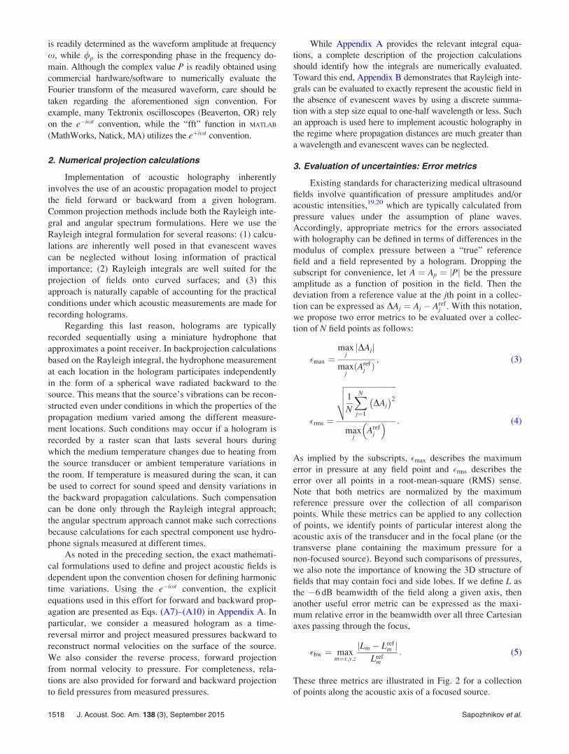
These three metrics are illustrated in Fig. 2 for a collection

of points along the acoustic axis of a focused source.

1518 J. Acoust. Soc. Am. 138 (3), September 2015 Sapozhnikov et al.

B. Test configurations for virtual experiments

Simulations were used to conduct virtual experiments to

quantify the errors associated with field sampling and sys-

tematic uncertainties in the position/timing of measurements.

Considering a known source boundary condition, forward

projection was performed to determine the pressure field

available for measurement. By sampling this “true” field in

different ways, measured holograms were recorded and used

to reconstruct the field in two steps (see Fig. 1): First the

field was projected backward from the measured hologram

to a source surface. Then this source hologram was used to

project the field forward to some set of points

of interest. Finally, the error in the reconstructed field

was evaluated at these points in terms of the metrics from

Eqs. (3) to (5), using the original “true” field to define the

reference values.

To describe a virtual test configuration, it is necessary to

define both the “true” reference field and the method used to

sample this field to simulate a measured hologram. The first

two test configurations explore field sampling effects by

varying the aperture and axial position of the measured holo-

gram. For these simulations, two idealized sources were

considered to represent transducers used to generate intense

ultrasound for medical applications. Both transducers oper-

ate at 1 MHz and vibrate uniformly over a diameter of

10 cm. One transducer is a flat disk and the other is a spheri-

cal bowl with a 10 cm radius of curvature. Because the flat

disk and spherical bowl generate beams with different

shapes, consideration of both provides insight for selecting

the aperture and position of a measured hologram given

some presumed beam shape. For other test configurations,

only the spherically focused transducer was considered

because it represents the more complicated and interesting

case.

In all test configurations, beam propagation occurred

along the z axis (see Fig. 1), and the measured hologram was

defined from a square grid of measurements in a transverse

plane centered at z ¼ zh. The step size between measure-

ments in the grid was always k=2. As noted before, this sam-

pling is sufficient to fully represent the field in the absence

of evanescent waves. Source holograms were reconstructed

using a slightly smaller step size equal to k=3 to provide

improved visual resolution in images of the source. Beyond

the configurations that explicitly varied measurement

aperture and axial position, measured holograms were

evaluated in the plane zh ¼ 50 mm using an aperture of

2ah ¼ 150 mm. As determined from the initial simulations,

this relatively large aperture captured the full width of the

focused beam at zh ¼ 50 mm. Except for explicit simulations

of temperature uncertainties, all projection calculations used

the following properties for the propagation medium: density

q0 ¼ 1000 kg/m3 and sound speed c0 ¼ 1500 m/s. In the

following text, the methods used to simulate hologram

recording in different test configurations are described in

further detail.

1. Aperture and axial position of the measuredhologram

To assess the role of hologram aperture 2ah on accuracy,

simulations were performed for both the flat and focused

transducers. The measured hologram was recorded at

zh ¼ 50 mm for apertures ranging from 10 to 150 mm. Given

the transducer aperture D, hologram apertures ranged from

0.1D to 1.5D. In addition, simulations for both transducers

were conducted to evaluate the impact of the axial location

of the measured hologram. Using apertures of both 50 and

150 mm, the measured hologram was recorded at positions

zh ranging from 40 to 160 mm, thereby covering pre-focal

through post-focal positions for the spherically focused

transducer.

2. Hydrophone size

When a pressure field is measured by a hydrophone of

finite size, the measured signal is proportional the average

normal velocity of fluid particles impinging on the hydro-

phone’s measuring surface. Accordingly, the hydrophone

will possess different sensitivities for plane waves arriving

from different directions. Such behavior can affect hologra-

phy measurements. To investigate these effects, we utilize

the reciprocity theorem for acoustic waves. This theorem

states that the hydrophone sensitivity to waves arriving from

different directions can be inferred from the directivity

pattern of the hydrophone when it is used as a source. Thus

measured hydrophone signals can be simulated by multiply-

ing the complex amplitude of each incoming wave by the

relevant directivity value.

Let us consider a hydrophone with a flat, circular sens-

ing element of radius a0. If we assume that the hydrophone

FIG. 2. Definition of holographic reconstruction errors for a collection of

points. The top plot shows the axial distribution of pressure magnitude for a

uniform, focused source as determined by reference calculations and field

reconstruction from a hologram. The �6 dB “beamwidth” corresponding to

each field is labeled; these values are used to calculate the error metric �bw.

The bottom plot shows the deviation between the two fields in terms of both

a peak value �max and an average value �rms. Both of these error metrics are

normalized by the maximum reference pressure magnitude over the collec-

tion of points considered.

J. Acoust. Soc. Am. 138 (3), September 2015 Sapozhnikov et al. 1519

radiates as a circular piston source, the corresponding direc-

tivity pattern is known to be

D hð Þ ¼ 2 J1 ka0 sin hð Þka0 sin h

: (6)

Here J1ð�Þ is the first-order Bessel function, k ¼ x=c0 is the

wavenumber, and h is the angle between the hydrophone’s

axis of symmetry and the direction from which the plane

wave arrives. To account for the hydrophone directivity in

the angular spectrum approach, the measured field can be

simulated by multiplying the angular spectrum amplitudes

by DðhÞ, where sin h ¼ffiffiffiffiffiffiffiffiffiffiffiffiffiffiffik2

x þ k2y

q=k and the notation defin-

ing spatial frequencies kx, ky is given in Appendix B.

When holography is based on the Rayleigh integral,

hydrophone directivity can also be simulated in a simple

way if the ultrasound source points are in the far field of the

hydrophone (i.e., the propagation distance to the hydro-

phone is much larger than the near-field scale ka20=2). This

condition is usually met especially for hydrophones with

small sensing elements. Here we use the directivity factor

to simulate how the true field would be measured by a

hydrophone of finite size. Then directivity effects are

neglected in subsequent field reconstructions. More specifi-

cally, forward projection from an idealized source based on

Eq. (A7) or (A8) in Appendix A is performed by multiply-

ing the relevant integrand by DðhÞ. Note that sin h and DðhÞcan be evaluated directly as a function of the position vec-

tors r1 and r2 for each point inside the surface integral (see

Fig. 13). Using Cartesian coordinates ðx1; y1; z1Þ and

ðx2; y2; z2Þ to describe points on surfaces R1 and R2, respec-

tively, we have

sin h ¼

ffiffiffiffiffiffiffiffiffiffiffiffiffiffiffiffiffiffiffiffiffiffiffiffiffiffiffiffiffiffiffiffiffiffiffiffiffiffiffiffiffiffiffiffiffiffix2 � x1ð Þ2 þ y2 � y1ð Þ2

qffiffiffiffiffiffiffiffiffiffiffiffiffiffiffiffiffiffiffiffiffiffiffiffiffiffiffiffiffiffiffiffiffiffiffiffiffiffiffiffiffiffiffiffiffiffiffiffiffiffiffiffiffiffiffiffiffiffiffiffiffiffiffiffiffiffiffiffiffiffix2 � x1ð Þ2 þ y2 � y1ð Þ2 þ z2 � z1ð Þ2

q : (7)

This approach was used to simulate directivity effects in

recorded holograms for hydrophones with sensing diameters

up to 2 mm.

It is instructive to note that errors associated with hydro-

phone directivity can be accounted for in subsequent recon-

structions if the directivity pattern is known. The integrand

used in backprojection calculations is simply divided by

DðhÞ. However, for hydrophones that are large relative to the

propagation wavelength, averaging over the face of the

hydrophone will limit the amount of information that can be

recorded. In other words, the directivity pattern will include

values near zero for large hydrophones, thereby limiting the

ability to record holograms from which the full field can be

reconstructed.

3. Non-orthogonality between scan axes

Holography measurements are typically made by mov-

ing a single hydrophone in a plane with the help of an auto-

mated 3D positioner. If the positioner axes used to move the

hydrophone are not exactly orthogonal, then the locations

of the measurements will be systematically incorrect. To

explicitly describe these conditions, it is convenient to intro-

duce two sets of Cartesian coordinates: (x, y, z) coordinates

aligned to the source transducer and ðx0; y0; z0Þ coordinates

aligned to the axis of a 3D positioner. We take the z axis to

coincide with beam propagation as in Fig. 1 with the origin

at the transducer apex. In contrast, we naturally assign the

origin of the primed positioner coordinates to correspond to

some reference point along the beam axis such as the acous-

tic focus. Here we assume that the z and z0 axes are perfectly

aligned and consider the impact of a lack of orthogonality

between the x0 and y0 axes. We simulate the case in which

the recorded hologram assumes that the scan axes x0 and y0

are orthogonal to one another even though the actual angle

between them is 90� þ axy. Accordingly, we consider a scan

over some desired range of ðx0; y0Þ coordinates and sample

the true field at the locations actually accessed by the posi-

tioner: x ¼ x0 � y0 sin axy and y ¼ y0 cos axy. Simulations

were performed for 0� � axy � 3�.

4. Non-orthogonality between the scan planeand the beam propagation axis

Another situation of practical interest occurs when none

of the positioner axes are perfectly aligned with the z axis,

which is defined to coincide with the direction of beam prop-

agation. If we consider the same coordinates aligned to the

transducer (x, y, z) and the positioner ðx0; y0; z0Þ, these condi-

tions can be described by a nonzero angle az between the zand z0 axes. In this case, the scan plane defined by the

ðx0; y0; z0 ¼ 0Þ plane that intersects the beam axis at z ¼ zh

will not be orthogonal to beam propagation in the zdirection.

To simulate such a coordinate misalignment, the meas-

ured hologram is determined by sampling the true field over

a desired range of positioner coordinates in the x0y0 plane.

For an axisymmetric transducer, the orientation of the tilt

angle az does not matter. For convenience, we consider the

misalignment as a rotation of the scan plane around the yaxis,

xy

z� zh

24

35 ¼ cos az 0 sin az

0 1 0

�sin az 0 cos az

0@

1A x0

y0

z0 ¼ 0

24

35: (8)

In this way, angular misalignment of the scan plane was

simulated for 0� � az � 3�. The errors associated with this

misalignment were then evaluated by assuming az ¼ 0 in

field reconstruction calculations. Although this type of mis-

alignment causes errors, we note that the measured hologram

still captures the correct 3D field structure; this structure is

simply rotated. Accordingly, errors caused by this misalign-

ment can be corrected if the rotation is known.

5. Constant temperature errors

In holography, field reconstruction calculations rely on

known characteristics of the propagation medium, namely,

the density q0 and sound speed c0. Although these properties

are well known for water, they vary with temperature.

For any measured hologram, the temperature of the water

1520 J. Acoust. Soc. Am. 138 (3), September 2015 Sapozhnikov et al.

should therefore be measured to facilitate accurate field

reconstructions. However, temperature measurements may

be inaccurate or even omitted from the data collection. In

such cases, we seek to quantify how field reconstructions are

affected when the temperature used for projection calcula-

tions differs by a constant amount from the actual tempera-

ture during measurement acquisition.

To simulate such conditions, forward projections of the

“true” field were performed with default properties q0 ¼1000 kg/m3 and c0 ¼ 1500 m/s; subsequent projection calcu-

lations then presumed an erroneous temperature described

by the constant shift DT0, using corresponding shifts in den-

sity and sound speed. For water between 20 �C and 30 �C,

variations of these properties with temperature are approxi-

mately linear.35–37 Accordingly, modified properties were

calculated as q0½kg=m3� ¼ 1000� 0:25DT0 and c0½m=s�¼ 1500þ 2:5DT0, where DT0 is expressed in degrees

Celsius. Simulations considered temperature errors over the

range �4�C � DT0 � 4�C.

6. Temperature drift during a raster scan

Another consideration related to temperature uncer-

tainty in the propagation medium is the potential for

temperature changes during the acquisition of holography

measurements, which can take several hours. To simulate

such conditions, we assume that measurements are acquired

by making a raster scan and that the temperature changes the

same amount between consecutive measurement points. For

total temperature drift DTd, the temperature change for the

nth measurement point in a scan containing N total points is

then DTd � ðn� 1Þ=N; the temperature shift at each point

was used to determine the corresponding density and sound

speed from the linear relations given in the preceding text.

Errors due to temperature drift were assessed by considering

the temperature changes in the forward projection of the

“true” field, while subsequent reconstruction calculations

used the default values q0 ¼ 1000 kg/m3 and c0 ¼ 1500 m/s.

Simulations covered the range �4�C � DTd � 4�C.

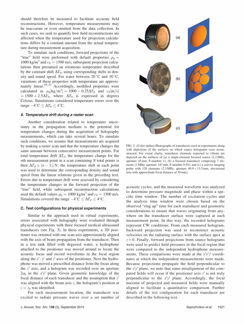
C. Test configurations for physical experiments

Similar to the approach used in virtual experiments,

errors associated with holography were evaluated through

physical experiments with three focused medical ultrasound

transducers (see Fig. 3). In these experiments, a 3D posi-

tioner was oriented with one scan axis approximately aligned

with the axis of beam propagation from the transducer. Then

in a test tank filled with degassed water, a hydrophone

attached to the positioner was moved around to locate the

acoustic focus and record waveforms in the focal region

along the x0; y0 and z0 axes of the positioner. Next the hydro-

phone was moved a prescribed distance from the focus along

the z0 axis, and a hologram was recorded over an aperture

2ah in the x0y0 plane. Given geometric knowledge of the

focal distance of each transducer and the assumption that z0

was aligned with the beam axis z, the hologram’s position at

z ¼ zh was identified.

For each measurement location, the transducer was

excited to radiate pressure waves over a set number of

acoustic cycles, and the measured waveform was analyzed

to determine pressure magnitude and phase within a spe-

cific time window. The number of excitation cycles and

the analysis time window were chosen based on the

observed “ring up” time for each transducer and geometric

considerations to ensure that waves originating from any-

where on the transducer surface were captured at each

measurement point. In this way, the recorded holograms

represent CW conditions. From each measured hologram,

backward projection was used to reconstruct acoustic

velocities on the radiating surface with the surface apex at

z¼ 0. Finally, forward projections from source holograms

were used to predict field pressures in the focal region that

were compared to the independent hydrophone measure-

ments. These comparisons were made at the x0y0z0 coordi-

nates at which the independent measurements were made.

Because projections propagate the field perpendicular to

the x0y0 plane, we note that some misalignment of the com-

pared fields will occur if the positioner axis z0 is not truly

perpendicular to the x0y0 plane. Accordingly, the focal

maxima of projected and measured fields were manually

aligned to facilitate a quantitative comparison. Further

details of the test configuration for each transducer are

described in the following text.

FIG. 3. (Color online) Photographs of transducers used in experiments along

with depictions of the surfaces on which source holograms were recon-

structed. For visual clarity, transducer elements expected to vibrate are

depicted on the surfaces of (a) a single-element focused source (2.2 MHz,

aperture 45 mm, F-number 1); (b) a focused transducer comprising 7 ele-

ments (1 MHz, aperture 147 mm, F-number 0.95); and (c) a convex imaging

probe with 128 elements (2.3 MHz, aperture 49.9� 13.5 mm, elevational

lens with approximate focal distance of 50 mm).

J. Acoust. Soc. Am. 138 (3), September 2015 Sapozhnikov et al. 1521

1. Single-element transducer

One test transducer comprised a single, spherically

curved ceramic element operating frequency of 2.2 MHz. All

measurements were made at Moscow State University using

a capsule hydrophone (GL-0150-1 A, Specialty Engineering

Acoustics, Soquel, CA) with a sensitivity at 2.2 MHz of

0.21 lV/Pa and a sensing region with diameter 0.15 mm. The

scan was executed using a Velmex (Bloomfield, NY) posi-

tioning system comprising stepper motors and linear slides

with a combined positioning resolution of 2.5 lm/step along

each axis. At each measurement location, the pressure wave-

form was recorded by a digital oscilloscope (Tektronix

TDS520A, Beaverton, OR). Additional details describing the

transducer, the measured hologram, and projection calcula-

tions are listed under transducer (a) in Table I. Although the

water temperature was not measured directly during measure-

ments, sound speed was measured as c0 ¼ 1495:7 m/s, imply-

ing temperature T0 ¼ 24:7 �C and density q0 ¼ 996:9 kg/m3.

These values were used in all projection calculations.

2. Seven-element therapy array

The second test transducer was an array of seven flat

disks, each 50 mm in diameter. The disks were bonded to a

plastic shell, which was shaped to provide an integral acous-

tic lens for each disk. The lenses focused the field generated

by each disk at a distance of 140 mm, and the overall contour

of the shell aligned the foci of all seven disks to overlap.

Overall geometric details of the transducer and measure-

ments are given under transducer (b) in Table I. All measure-

ments were made at the University of Washington using a

capsule hydrophone (HGL-0200, Onda Corp., Sunnyvale,

CA) with a sensitivity at 1 MHz of 0.42 lV/Pa and a sensing

region with diameter 0.2 mm. The scan was executed using a

Velmex positioning system with stepper motors and linear

slides that provided a resolution of 6 lm per step. The pres-

sure waveform at each location was recorded using a digital

oscilloscope (DSO-X 3034A, Keysight Technologies, Inc.,

Santa Rosa, CA). For holography measurements, the trans-

ducer output level was 1.95 times higher than that used for

the independent focal measurements; this elevated output

level was used to improve signal-to-noise without the need

for waveform averaging at each location. The water proper-

ties were not measured directly; instead, a temperature

near 20 �C was assumed, with values c0 ¼ 1485 m/s and

q0 ¼ 998 kg/m3 used in all projection calculations.

3. Convex imaging probe

The third test transducer was a convex imaging probe

driven at 2.3 MHz. The transducer is a phased array consist-

ing of 128 elements with a convex radius of curvature of

about 38.5 mm. Elements were phased to generate a beam

focused along the central axis of the transducer, 53 mm

beyond its apex. Further geometric details of the transducer

and measurements are given under transducer (c) in Table I.

All measurements were made at the University of

Washington using the same instrumentation as described in

the preceding text for the seven-element (b) transducer with

a hydrophone sensitivity of 0.40 lV/Pa at 2.3 MHz. Again, a

higher transducer output level (22.3 times higher) was used

for holography measurements to increase the relative signal

amplitude without averaging.

III. RESULTS

A. Virtual experiments

The results from virtual experiments are presented in

Figs. 4–10, which show how various parameters affect the

accuracy of holographic field reconstructions. Each figure

plots one or more error metrics as a function of a parameter

that quantifies the amount of uncertainty introduced by a

practical implementation of acoustic holography. Field

points included in the error evaluations are as follows:

Points in the xy plane for �75 � x; y � 75 mm with a step

size of 0.75 mm; points along the z axis from 40 to 160 mm

with a step size of 0.075 mm. Each figure also includes

reconstructed source holograms for two specific parameter

values to provide some physical insight into the ways in

which the associated errors distort the effective source and

the field it radiates.

1. Field sampling errors

A fundamental approximation related to practical imple-

mentations of acoustic holography is representation of the

whole field by a discrete set of measurements. As noted in

Sec. I and in Sec. II A 2, we neglect evanescent waves and

therefore can discretize the field without loss of information

using a step size between measurements of one-half wave-

length. However, because the measurement aperture 2ah

must be finite, sampling errors are introduced that depend on

this aperture and the relative position zh of the measured

hologram.

In Fig. 4, accuracy as a function of measurement aper-

ture at zh ¼ 50 mm is depicted for the flat transducer

described in Sec. II B. As expected, the error metrics �max

and �rms decrease as the measurement aperture gets larger.

TABLE I. Experimental holography parameters.

Transducer from Fig. 3

(a) (b) (c)

Frequency (MHz) 2.2 1 2.3

Transducer aperture (mm) 45 147 49:9� 13:5

Focal distance (mm) 45 140 53

zh (mm) 30 85 38

Measurement aperture 2ah (mm) 30� 30 120� 120 199:5� 40:6

step size (mm) 0.30 0.75 0.35

No. scan points 10 201 25 921 66 807

No. excitation cycles 120 60 160

Time window (ls) 42–44 104–114 88–98

Hydrophone size 2a0 (mm) 0.15 0.2 0.2

q0 (kg/m3) 997 998 998

c0 (m/s) 1496 1485 1485

Source surface aperture (mm) 58:8� 58:8 176:8� 176:8 62:8� 26:4

Source step size (mm) 0.2 0.4 0.2

1522 J. Acoust. Soc. Am. 138 (3), September 2015 Sapozhnikov et al.

Considering the more sensitive metric �max and a target error

level of 1% (which is about an order of magnitude less than

the uncertainty of hydrophone calibration), a hologram aper-

ture greater than 130 mm is sufficient. Although not shown,

a comparable plot for the spherically focused transducer

demonstrates that a hologram at zh ¼ 50 mm requires an

aperture greater than 68 mm to keep �max less than 1%.

Considering the respective beam geometries of these two

sources as a cylinder and a cone, we note that a hologram

aperture of about 1.3 times the beam diameter is sufficient to

achieve sampling error less than 1%. While this rule of

thumb can be useful at axial positions relatively close to the

source, it loses meaning elsewhere. For example, it is

unclear how the rule might apply in the focal plane of a

spherically curved source where the geometric beam diame-

ter vanishes.

To explore the impact of the axial measurement position

zh, Fig. 5 shows �max and �bw for the focused source for both

a small measurement aperture (2ah ¼ 50 mm, solid lines)

and a large one (2ah ¼ 150 mm, dashed lines). If measure-

ments are made near the focus where the beam is narrow, it

is clear that even a small measurement aperture can accu-

rately capture details in the focal plane. However, corre-

sponding errors on axis grow significantly because waves

emanating from the edge of the source are missed by a small

scan plane, and these edge waves interfere constructively/

destructively to cause peaks/nulls on axis. This result dem-

onstrates that a hologram should capture as much energy as

possible from the incident beam to accurately represent the

field. Because some waves always diverge from the source,

measurements should generally be made fairly close to the

source. Indeed analogous simulations for the flat transducer

show that errors remain less than 1% only when the large

measurement aperture (2ah ¼ 150 mm) is positioned at zh �75 mm. For both transducers, results suggest that as long as

the hologram is large enough to capture most of the radiated

wave energy, its exact position is not critical.10 For a focused

source, Fig. 5 demonstrates that a hologram positioned about

halfway between the source and focus is useful to achieve

small field reconstruction errors with a minimal number of

measurements; however, the axial position of measurements

can be selected to accommodate a given experimental

arrangement if the measurement aperture is also adjusted.

A final aspect of field sampling is the finite size of the

hydrophone used to record measurements. Although such

errors can be corrected by including reciprocal directivity

effects in subsequent projection calculations, such

FIG. 4. (Color online) Field reconstruction errors (top) for the flat source

(100 mm aperture) as a function of the size of the measurement region. This

region is a square 2ah � 2ah with its center placed on the acoustic axis at

zh ¼ 50 mm. Bottom images illustrate the reconstructed source hologram in

terms of velocity magnitude and phase distributions for two possible sizes of

the measurement region (corresponding measurement apertures are circled).

FIG. 5. (Color online) Field reconstruction errors (top) for the focused

source (100 mm aperture) as a function of the axial position zh of the mea-

surement region. Solid lines correspond to a measurement region with aper-

ture 2ah ¼ 50 mm; dashed lines correspond to a region with aperture

2ah ¼ 150 mm. Bottom images illustrate source holograms reconstructed

using the smaller measurement aperture at the indicated axial measurement

positions.

J. Acoust. Soc. Am. 138 (3), September 2015 Sapozhnikov et al. 1523

corrections are neglected here. Simulation results are pre-

sented in Fig. 6, demonstrating that errors remain less than

1% if the hydrophone diameter remains less than about a

quarter wavelength (k=4). As depicted in the reconstructed

source holograms, uncorrected directivity effects diminish

the relative contributions from peripheral regions of the

transducer.

Given the results presented in Figs. 4 and 5, simulations

to explore the impact of other parameters were conducted

for measurements with aperture 2ah ¼ 150 mm and axial

location zh ¼ 50 mm for the focused transducer. In addition,

virtual measurements were simulated for the idealized case

of an infinitesimally small hydrophone.

2. Geometrical errors

Additional errors associated with holography can be

attributed to uncertainties in the positions at which measure-

ments are made. In most experimental configurations, a holo-

gram is recorded by a scan over two linear axes that define the

x0y0 plane. Although it is typically assumed that the scan axes

are perpendicular in defining the coordinate locations of meas-

urements, there will be some error in practice. The impact of

such errors is quantified in Fig. 7 as a function of axy, the

angular deviation from perpendicularity. Results show that

errors are less than 1% if the scan axes remain within about

0.4� of perpendicularity. Note that even if such alignment is

not achieved, errors can be corrected as long as the actual

angle between scan axes is known. Although positioners

designed for optics often specify axis alignment tolerances

much smaller than 0.4�, other industrial positioners lack such

specifications and rely on end users to assemble two or more

linear stages. In such cases, alignment error is likely governed

by the clearance tolerances for the bolts and holes used in as-

sembly. Based on typical designs for linear stages and stand-

ard machining practices for clearances,38 it is plausible that

alignment errors on the order of 0.5� could occur.

Another source of geometric uncertainty is the orienta-

tion of the x0y0 scan plane relative to the beam axis. Figure 8

illustrates the errors caused by rotation of the scan plane

relative to the beam axis when this rotation is neglected in

subsequent projection calculations. As is clear from the

reconstructed source holograms, the primary effect of mis-

alignment is to make the phase non-uniform at the radiating

surface, effectively steering the beam off axis. Although

calculated errors are quite sensitive to this type of axial mis-

alignment, such error values are somewhat artificial in that

transducer-aligned coordinates were explicitly substituted

for positioner-aligned coordinates. Such confusion can be

FIG. 6. (Color online) Field reconstruction errors (top) for the focused

source as a function of the diameter of the hydrophone’s sensing element.

The measurement region is located at zh ¼ 50 mm with aperture 2ah ¼ 150

mm. Bottom images illustrate reconstructed source holograms for the indi-

cated hydrophone diameters.

FIG. 7. (Color online) Field reconstruction errors (top) for the focused

source as a function of the skew angle relative to 90� of the transverse x0y0

coordinate axes used in capturing measurements within the scan plane. The

measurement region is at zh ¼ 50 mm with aperture 2ah ¼ 150 mm. Bottom

images illustrate reconstructed source holograms for the indicated skew

angles.

1524 J. Acoust. Soc. Am. 138 (3), September 2015 Sapozhnikov et al.

readily avoided in practice given that the measured hologram

contains the full 3D beam structure.

As noted by Kreider et al.,28 the orientation of the beam

axis relative to measurement coordinates can be inferred from

the position of the focus as determined by forward projection

from the measured hologram. If the focus does not lie along the

positioner’s z0 axis, then the beam and positioner are not aligned

and the alignment angle can be determined. Moreover, for both

focused and unfocused sources, the angular orientation of the

source hologram can be estimated by reconstructing acoustic

phase on source surfaces with different orientations relative to

the hologram. The true source orientation can then be identified

as the one that yields a distribution of phase over the transducer

surface that is uniform or follows the transducer’s geometric

symmetry (e.g., see Fig. 11). These approaches were used in

Ref. 28 to verify the relative orientation of the measured

hologram within about 0.2�. We conclude that the actual

alignment of the scan plane is not critical in practice as long as

the scanned region is approximately transverse to the beam and

large enough to “catch” most of the radiated energy (see Fig. 5).

3. Temperature errors

Because holography implicitly relies on projection cal-

culations, a final type of error in the reconstructed fields is

related to uncertainties in the acoustic properties of the prop-

agation medium (i.e., water). The relevant properties are

sound speed and density, which vary as a function of temper-

ature under practical measurement conditions. If a hologram

is recorded at one temperature and subsequent projection

calculations utilize a different temperature, the reconstructed

field will differ from the original one. Beyond such a static

temperature bias, other errors can accrue if the temperature

drifts during measurements and projection calculations uti-

lize a single temperature. Errors associated with these types

of temperature uncertainties are plotted in Figs. 9 and 10,

which show that the temperature uncertainty should remain

within 61 �C to keep errors less than about 1%.

B. Physical experiments

To evaluate the accuracy of holography in practice,

physical experiments were conducted with the three trans-

ducers depicted in Fig. 3. Measurement and reconstruction

parameters are listed in Table I; the reconstructed fields for

each transducer were compared to independent hydrophone

measurements acquired as line scans through the focus. As

such, comparisons were made at the following field points

along the z0 axes:

FIG. 8. (Color online) Field reconstruction errors (top) for the focused

source as a function of the angular misalignment between the source’s

acoustic axis and the direction normal to the scan plane. The measurement

region is at zh ¼ 50 mm with aperture 2ah ¼ 150 mm. Bottom images illus-

trate reconstructed source holograms for the indicated misalignment angles.

FIG. 9. (Color online) Field reconstruction errors (top) for the focused

source as a function of the uncertainty in temperature at which the field

measurements were made. This uncertainty is presumed to comprise a con-

stant bias in the sound speed used in reconstructing the source hologram.

The measurement region is located at zh ¼ 50 mm with aperture 2ah ¼ 150

mm. Bottom images illustrate reconstructed source holograms for the indi-

cated temperature biases.

J. Acoust. Soc. Am. 138 (3), September 2015 Sapozhnikov et al. 1525

(a) Single-element transducer: 20 � z0 � 90 mm, 0.5 mm

step size,

(b) Seven-element therapy array: 109 � z0 � 169 mm,

0.1 mm step size,

(c) Convex imaging probe: 33 � z0 � 73 mm, 0.2 mm step

size.

Reconstructed source holograms are shown in Fig. 11.

For transducers (a) and (b), surface waves are clearly evident

in the form of concentric rings on each ceramic element. For

transducer (c), the phase plot shows the effects of both a

cylindrical lens for focusing in the elevation direction and

element phasing for on-axis focusing in the azimuthal direc-

tion. In addition, the magnitude plot shows reduced vibration

amplitudes off-axis in the azimuthal direction. This result

can be explained by phase averaging: The reconstruction has

a spatial resolution on the order of k=2, which is larger than

the actual width of each array element. Accordingly, when

adjacent elements vibrate with different phases, averaging of

these phases across the elements yields an apparent reduc-

tion in magnitude. Despite this phase averaging, the source

hologram has sufficient resolution to accurately represent the

field that is radiated more than a few wavelengths away from

the transducer.

FIG. 10. (Color online) Field reconstruction errors (top) for the focused

source as a function of the amount of temperature drift that occurs during

the acquisition of measurements by a raster scan. Temperature is assumed to

change linearly with the scan point number. The measurement region is at

zH ¼ 50 mm with aperture 2ah ¼ 150 mm. Bottom images illustrate recon-

structed source holograms for the indicated temperature changes.

FIG. 11. (Color online) Source holograms reconstructed from experimental

measurements for the three sources depicted in Fig. 3. Note that velocity

magnitudes are normalized relative to the maximum value in the hologram.

FIG. 12. (Color online) Comparison of axial fields measured directly versus

those projected from a measured hologram for the three sources depicted in

Fig. 3.

1526 J. Acoust. Soc. Am. 138 (3), September 2015 Sapozhnikov et al.

Direct comparisons of holographic projections with

independent measurements along the z0 axis are plotted in

Fig. 12. These plots show that the measured holograms

capture on-axis field structures with a high level of detail. To

quantify the accuracy, the values of error metrics �max; �rms,

and �bw are provided in Table II for points along the z0 axis.

For comparison, the table also reports errors from simulated

experiments in which the size and axial location of the

measured hologram are considered (note that in all cases, the

largest simulated errors occur along the z axis).

The largest holography errors along the z0 axis in physi-

cal experiments occurred for transducer (a) with �max 5%.

For the other transducers, the values of �max were smaller at

2%–3%. We note that the simulated errors follow the same

trend with the largest �max of 3.5% for transducer (a).

Plausible uncertainties of 1� C–2 �C in water temperature

may have contributed several percent error to �max, espe-

cially because neither temperature nor sound speed was

measured directly for transducers (b) and (c). Moreover,

uncertainty in the angle between scan axes axy may have also

contributed to experimental error.

Although the holographically reconstructed and inde-

pendently measured axial fields agree very well, it is instruc-

tive to note that field reconstructions in the transverse x0 and

y0 directions can be more sensitive to sources of error not

considered in the simulations. For instance, positioning

errors can occur due to “dropped” steps when motion is

driven by stepper motors without feedback from position

encoders. Such errors are particularly likely during trans-

verse scans that comprise a large number of points. We

noticed such a problem during transverse scans with trans-

ducer (a) for which �max in the focal plane rose as high as

about 20% for points in regions of steep field gradients. This

experience demonstrates that special attention should be

given to positioner reliability in the test configuration.

IV. CONCLUSIONS

Holography is a technique that permits a steady-state 3D

wave field to be collapsed to pressure measurements of mag-

nitude and phase made in 2D. Accordingly, a hologram is an

important characteristic of any source because it directly

reflects the vibratory behavior of the radiating surface of the

transducer. In this effort, we have presented a detailed for-

mulation of acoustic holography that relies on the Rayleigh

integral to perform field projection calculations. This formu-

lation neglects evanescent waves, utilizing the typical condi-

tions in medical ultrasound where holograms are measured

more than a few wavelengths from the source and projection

calculations involve similarly long propagation distances.

This formulation has several explicit benefits: Arbitrary

geometries, including curved surfaces, can be handled trans-

parently; projection calculations are inherently stable; and

point-by-point corrections are possible for temperature

changes in the propagation medium.

Beyond the basic holography formulation, we have

defined explicit metrics for comparing two ultrasound fields.

By comparing holographically reconstructed fields to corre-

sponding reference fields, we have used the metrics to quan-

tify holography errors in both simulated and physical

experiments. Simulated experiments demonstrate that meas-

ured holograms can represent reference ultrasound fields

with maximum errors on the order of 1%. These results

provide useful guidance on the selection of fundamental

measurement parameters: The measurement aperture should

be about 30% wider than the geometric width of the acoustic

beam, and measurements should be made with a relatively

small hydrophone (sensing diameter less than about k=4) to

avoid the need for directivity corrections. Other errors

related to uncertainties in the timing and position of meas-

urements can be larger than 1% in practice; however, such

errors can be minimized by measurement of the water

temperature during experiments and/or calibration of the

alignment of the 3D positioner axes.

For physical experiments, fields reconstructed from

measured holograms were compared with independent

hydrophone measurements for three different ultrasound

transducers. The maximum error on axis was 3% for two of

the transducers and 5% for the third. Although it is beyond

the scope of this effort to fully trace the sources of experi-

mental error, it is plausible that errors of 5% can be

explained by experimental details not fully taken into

account, including changes in the water temperature and

misalignment of positioner axes in the scan plane. Overall,

these experimental errors associated with holography are

comparable to those reported by Clement and Hynynen.8

Although Clement and Hynynen used a different normaliza-

tion for their error metric, we find their metric to be compa-

rable to �max for our data.

Future work will aim to further identify sources of

experimental error. Our results suggest that reconstruction

errors in the focal plane can be particularly sensitive to hard-

ware positioning errors, thereby demonstrating the impor-

tance of ensuring consistent hardware performance during

large scans. However, even for the case with the largest

errors, Figs. 11 and 12 demonstrate that the measured holo-

gram captures many details of the source vibrations and the

corresponding radiated field. In total, the results of the physi-

cal experiments validate the two main assumptions behind

the holography formulation: the neglecting of evanescent

waves and the adaptation of calculations to non-flat surfaces.

TABLE II. Holography errors associated with physical experiments.

From experiments From simulations

(z0 axis) (z axis)

(a) Single-element transducer

�max 0.053 0.035

�rms 0.018 0.005

�bw 0.003 <0.001

(b) Seven-element array

�max 0.024 <0.001

�rms 0.011 <0.001

�bw 0.018 <0.001

(c) Convex imaging probe

�max 0.033 0.013

�rms 0.014 0.004

�bw 0.017 0.007

J. Acoust. Soc. Am. 138 (3), September 2015 Sapozhnikov et al. 1527

A basic goal of this work was to develop a methodology

for designing holography measurements that meet specified

error criteria. By presenting such an approach along with

practical implementation guidelines, this work advances

acoustic holography as a metrological tool. In medical ultra-

sound, such capabilities can simplify the characterization of

therapeutic fields,20 which can otherwise involve an extraor-

dinary number of measurements. Beyond field characteriza-

tion per se, holography provides unique functionality in that

it permits reconstruction of the vibrations at the transducer

surface. Quantifying these vibrations can be useful for opti-

mizing and/or monitoring transducer performance as well as

for defining a boundary condition for forward projection

models that include nonlinear propagation in tissue.

ACKNOWLEDGMENTS

The authors thank our collaborators at the Center for

Industrial and Medical Ultrasound. In particular, we thank Mr.

Bryan Cunitz, Dr. Adam Maxwell, Dr. Michael Bailey, and

Dr. Yuri Pishchal’nikov for efforts related to the acquisition of

experimental data. This work was supported by the National

Institutes of Health (R21EB016118, R01EB007643,

P01DK43881) and the National Space Biomedical Research

Institute through NASA NCC 9-58. Experimental

measurements performed at Moscow State University were

supported by the Russian Science Foundation (14-15-00665).

APPENDIX A: RAYLEIGH INTEGRAL FORMULAS

Here we describe explicitly the expressions that were

used in reconstructing acoustic fields from holograms. We

begin by assuming linear, lossless acoustic propagation in a

medium with density q0 and sound speed c0. Then the prob-

lem can be formulated by considering a source located on a

boundary surface R1 as depicted in Fig. 13. The outgoing

wave field satisfies the Helmholtz equation

r2Pþ k2P ¼ 0; (A1)

where P denotes the complex pressure magnitude as defined

in Eq. (1), k ¼ x=c0 is the wavenumber, and x is the angular

frequency. Note that we have already introduced the e�ixt

convention, which affects the equations that follow. Use of

the eþixt convention instead would yield equivalent equa-

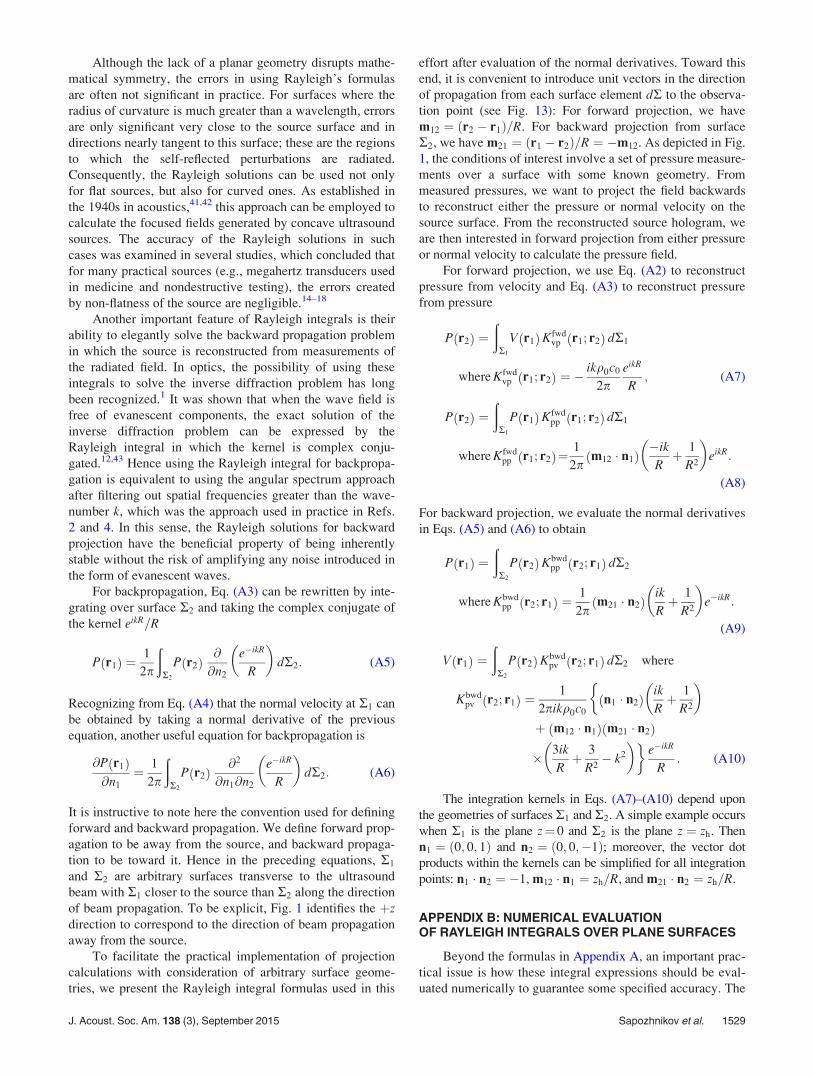
tions in which i is replaced by – i.If R1 denotes a plane surface with outward unit normal

n1 oriented in the direction of wave propagation, the exact

solution can then be expressed by Rayleigh’s integral formu-

las that follow from the Kirchhoff–Helmholtz integral,13

P r2ð Þ ¼ �1

2p

ðR1

@P r1ð Þ@n1

eikR

RdR1; (A2)

P r2ð Þ ¼1

2p

ðR1

P r1ð Þ@

@n1

eikR

R

� �dR1: (A3)

Here R ¼ jr2 � r1j is the distance between a given observa-

tion point at r2 and each surface element dR1 at position r1.

As such, R varies over the integrating surface R1 and the

normal derivative (@=@n1 ¼ n1 � rÞ denotes spatial differen-

tiation with respect to the outward normal n1 at the location

of each surface element dR1. Bouwkamp termed Eqs. (A2)

and (A3) the “Rayleigh solutions” and “Rayleigh’s first and

second formulas.”13 Note that in linear acoustics the normal

derivative of pressure is proportional to the component of

velocity in the same direction

@P

@n¼ ikq0c0V; (A4)

where V is a complex magnitude as defined in Eq. (2). At the

surface of a source, it is the normal velocity (not pressure)

that characterizes the surface vibrations. To match this phys-

ical interpretation, the term “Rayleigh integral” in the acous-

tics literature typically refers only to Eq. (A2), which is

written explicitly in terms of the normal velocity V.

For forward propagating waves, it can be shown that the

Rayleigh formulas are equivalent to the angular spectrum so-

lution of Eq. (A1).13,39 While the angular spectrum approach

is readily understood as a direct solution of the homogeneous

Helmholtz equation, the Rayleigh solutions have a clear

physical interpretation: They provide a rigorous mathemati-

cal foundation for the Huygens–Fresnel principle.40

Specifically, Eq. (A2) represents the radiated field as a super-

position of monopole sources emitting spherical waves

inside a bounded half space. Equation (A3) does the same as

a sum of dipole sources. Note that the Rayleigh solutions are

mathematically exact only for acoustic sources arranged on

a plane surface. Considering the Huygens–Fresnel interpreta-

tion, it is easy to understand this restriction: The original

spherical wave radiated by each differential source element

over the surface will “feel” the physical curvature, either

reflecting from other parts of a concave surface or diffracting

in the shadow of a convex surface.

FIG. 13. (Color online) As used for field projection calculations, two surfa-

ces R1 and R2 are depicted schematically relative to a coordinate system

with origin O. Each surface corresponds to the locus of points represented

by position vectors r1 or r2, respectively. R1 represents a boundary surface

with an acoustic source that radiates waves into the half-space region that

includes R2. This surface is further described by the outward facing unit nor-

mal n1 and differential area elements dR1. R2 is described by analogous

notation and represents a non-physical surface at which field measurements

are made.

1528 J. Acoust. Soc. Am. 138 (3), September 2015 Sapozhnikov et al.

Although the lack of a planar geometry disrupts mathe-

matical symmetry, the errors in using Rayleigh’s formulas

are often not significant in practice. For surfaces where the

radius of curvature is much greater than a wavelength, errors

are only significant very close to the source surface and in

directions nearly tangent to this surface; these are the regions

to which the self-reflected perturbations are radiated.

Consequently, the Rayleigh solutions can be used not only

for flat sources, but also for curved ones. As established in

the 1940s in acoustics,41,42 this approach can be employed to

calculate the focused fields generated by concave ultrasound

sources. The accuracy of the Rayleigh solutions in such

cases was examined in several studies, which concluded that

for many practical sources (e.g., megahertz transducers used

in medicine and nondestructive testing), the errors created

by non-flatness of the source are negligible.14–18

Another important feature of Rayleigh integrals is their

ability to elegantly solve the backward propagation problem

in which the source is reconstructed from measurements of

the radiated field. In optics, the possibility of using these

integrals to solve the inverse diffraction problem has long

been recognized.1 It was shown that when the wave field is

free of evanescent components, the exact solution of the

inverse diffraction problem can be expressed by the

Rayleigh integral in which the kernel is complex conju-

gated.12,43 Hence using the Rayleigh integral for backpropa-

gation is equivalent to using the angular spectrum approach

after filtering out spatial frequencies greater than the wave-

number k, which was the approach used in practice in Refs.

2 and 4. In this sense, the Rayleigh solutions for backward

projection have the beneficial property of being inherently

stable without the risk of amplifying any noise introduced in

the form of evanescent waves.

For backpropagation, Eq. (A3) can be rewritten by inte-

grating over surface R2 and taking the complex conjugate of

the kernel eikR=R

P r1ð Þ ¼1

2p

ðR2

P r2ð Þ@

@n2

e�ikR

R

� �dR2: (A5)

Recognizing from Eq. (A4) that the normal velocity at R1 can

be obtained by taking a normal derivative of the previous

equation, another useful equation for backpropagation is

@P r1ð Þ@n1

¼ 1

2p

ðR2

P r2ð Þ@2

@n1@n2

e�ikR

R

� �dR2: (A6)

It is instructive to note here the convention used for defining

forward and backward propagation. We define forward prop-

agation to be away from the source, and backward propaga-

tion to be toward it. Hence in the preceding equations, R1

and R2 are arbitrary surfaces transverse to the ultrasound

beam with R1 closer to the source than R2 along the direction

of beam propagation. To be explicit, Fig. 1 identifies the þzdirection to correspond to the direction of beam propagation

away from the source.

To facilitate the practical implementation of projection

calculations with consideration of arbitrary surface geome-

tries, we present the Rayleigh integral formulas used in this

effort after evaluation of the normal derivatives. Toward this

end, it is convenient to introduce unit vectors in the direction

of propagation from each surface element dR to the observa-

tion point (see Fig. 13): For forward projection, we have

m12 ¼ ðr2 � r1Þ=R. For backward projection from surface

R2, we have m21 ¼ ðr1 � r2Þ=R ¼ �m12. As depicted in Fig.

1, the conditions of interest involve a set of pressure measure-

ments over a surface with some known geometry. From

measured pressures, we want to project the field backwards

to reconstruct either the pressure or normal velocity on the

source surface. From the reconstructed source hologram, we

are then interested in forward projection from either pressure

or normal velocity to calculate the pressure field.

For forward projection, we use Eq. (A2) to reconstruct

pressure from velocity and Eq. (A3) to reconstruct pressure

from pressure

P r2ð Þ ¼ð

R1

V r1ð ÞKfwdvp r1; r2ð Þ dR1

where Kfwdvp r1; r2ð Þ ¼ �

ikq0c0

2peikR

R; (A7)

P r2ð Þ ¼ð

R1

P r1ð ÞKfwdpp r1; r2ð Þ dR1

where Kfwdpp r1; r2ð Þ¼

1

2pm12 � n1ð Þ

�ik

Rþ 1

R2

� �eikR:

(A8)

For backward projection, we evaluate the normal derivatives

in Eqs. (A5) and (A6) to obtain

P r1ð Þ ¼ð

R2

P r2ð ÞKbwdpp r2; r1ð Þ dR2

where Kbwdpp r2; r1ð Þ ¼

1

2pm21 � n2ð Þ

ik

Rþ 1

R2

� �e�ikR:

(A9)

V r1ð Þ ¼ð

R2

P r2ð ÞKbwdpv r2; r1ð Þ dR2 where

Kbwdpv r2; r1ð Þ ¼

1

2pikq0c0

n1 � n2ð Þik

Rþ 1

R2

� �þ m12 � n1ð Þ m21 � n2ð Þ

� 3ik

Rþ 3

R2� k2

� �e�ikR

R: (A10)

The integration kernels in Eqs. (A7)–(A10) depend upon

the geometries of surfaces R1 and R2. A simple example occurs

when R1 is the plane z¼ 0 and R2 is the plane z ¼ zh. Then

n1 ¼ ð0; 0; 1Þ and n2 ¼ ð0; 0;�1Þ; moreover, the vector dot

products within the kernels can be simplified for all integration

points: n1 � n2 ¼ �1, m12 � n1 ¼ zh=R, and m21 � n2 ¼ zh=R.

APPENDIX B: NUMERICAL EVALUATIONOF RAYLEIGH INTEGRALS OVER PLANE SURFACES

Beyond the formulas in Appendix A, an important prac-

tical issue is how these integral expressions should be eval-

uated numerically to guarantee some specified accuracy. The

J. Acoust. Soc. Am. 138 (3), September 2015 Sapozhnikov et al. 1529

first question that naturally arises is where measurements

should be acquired: If a measured hologram comprises a set

of discrete measurements made by scanning a hydrophone

over a plane, then what step size h between measurement

points should be used to enable accurate reconstruction of

the full field? Again using the geometry illustrated in Fig. 1,

we consider a measurements within the plane z ¼ zh, and use

x and y as the transverse coordinates that span the plane.

These measurements then define the complex magnitudes

Pðx; y; zhÞ, which can be used in the Rayleigh formulas.

Because we are using a version of holography in which

the region of interest is located many wavelengths away

from the source where evanescent waves are negligible,

there is no need for h to be less than a half wavelength. This

well-known result is based on the sampling theorem (i.e., the

Whittaker–Nyquist-Kotelnikov–Shannon theorem) as

applied to the angular spectrum of the field. The angular

spectrum can then be written in terms of the spatial sampling

frequencies kx and ky

Sðkx; ky; zhÞ ¼ð ðþ1�1

Pðx; y; zhÞe�iðkxxþkyyÞ dx dy : (B1)

In the absence of evanescent waves, a field with wavenum-

ber k ¼ 2p=k is fully represented by the portion of the

angular spectrum in the kx-ky plane that lies within the

circle k2x þ k2

y � k2. Consequently, the sampling theorem

can be applied to conclude that the field can be exactly

discretized with h � k=2 if evanescent waves are

neglected.

Although the sampling theorem guarantees that the

measurement spacing h ¼ k=2 is sufficient to fully cap-

ture the relevant part of the angular spectrum, it is still

not clear what spatial resolution should be used in the nu-

merical evaluation of Rayleigh integrals. It is instructive

to remember how a discretized data set can fully repre-

sent a continuous function. We assume that pressure P is

measured at discrete points in the xy plane with step size

h in both directions. As such, the coordinates (xm, yn) of

measurement locations can be expressed as xm¼mh,

yn¼ nh for m; n ¼ 0;61;62;…. While the number of

points is in practice limited, we assume negligible pres-

sure amplitudes beyond the measurement locations so

that an infinite number of points can be defined. Then

from the discretized pressure values Pmn ¼ Pðmh; nh; zhÞ,any value between the measured locations can be

obtained exactly by from the Whittaker–Shannon interpo-

lation formula,

P x; y; zhð Þ ¼X1

m¼�1

X1n¼�1

Pmn sinc px� mh

h

� �

� sinc py� nh

h

� �; (B2)

where sincðaÞ ¼ sin a=a.

In general, the continuous hologram Pðx; y; zhÞ may be

projected either backward to reconstruct the physical source

or forward to quantify the radiated field in three

dimensions. Here we model the diffraction behavior in

terms of forward projection to locations with z > zh.

Considering the form presented in both Eqs. (A3) and (A8),

Pðr1Þ is Pðx; y; zhÞ, and we seek to understand what discreti-

zation step size h0 should be used for numerical evaluation

of the integral. The answer depends on the proximity of the

observation point to the holography plane z ¼ zh. If it is

very close, the integration step h0 should be very small to

properly account for variation in the value of the kernel

[Eq. (A8)] over surface R1. However, using integration

steps h0 that are much smaller than the hologram step size his not a problem because Eq. (B2) allows exact resampling

wherever needed.

In the following text we explore when it is necessary to

use h0 h in the evaluation of Rayleigh integrals. When a

hologram is used to project the field over distances much

larger than a wavelength, we conclude that it is sufficient to

evaluate the integral as a summation with step size h0 ¼ h,

where h � k=2. As noted in Sec. I, the applications of

interest here do not involve evanescent waves or projection

distances on the order of a wavelength; hence, all integrals

were evaluated as simple summations with the step size

h0 ¼ h.

To prove this result regarding h0, we begin with a pres-

sure distribution Pðx; y; zhÞ that is represented by the angular

spectrum Sðkx; ky; zhÞ. Introducing Eq. (B2) into (B1), the

angular spectrum can be expressed as

S kx; ky; zhð Þ ¼X1

m¼�1

X1n¼�1

Pmn

ð1�1

sinc px� mh

h

� �

� e�ikxx dx

ð1�1

sinc py� nh

h

� �e�ikyy dy:

(B3)

Given that the integrals in the previous relation are Fourier

transforms, we note that a sinc function in the spatial domain

equates to a rectangular function in the frequency domain.

From this understanding, it is convenient to consider the

inverse transform

1

2p

ðp=h

�p=h

e�ikxmheikxx dkx

¼ 1

2peip x�mhð Þ=h � e�ip x�mhð Þ=h

ix¼ 1

hsinc p

x� mh

h

� �;

(B4)

from which we conclude that

ð1�1

sinc px� mh

h

� �e�ikxx dx

¼he�ikxmh for jkxj �

ph

0 for jkxj >ph:

8>><>>: (B5)

Now, we can rewrite Eq. (B3) as follows:

1530 J. Acoust. Soc. Am. 138 (3), September 2015 Sapozhnikov et al.

S kx; ky; zhð Þ ¼X1

m¼�1

X1n¼�1

h2Pmn e�i kxmhþikynhð Þ for jkxj �ph

and jkyj �ph

0 otherwise:

8><>: (B6)

At this point, it is convenient to remember that we are

only interested in fields that are free from evanescent

waves; in such cases, only spatial frequencies within the

circle k2x þ k2

y � k2 need to be considered. If p=h � k(i.e., h � k=2) as was originally assumed, then the angu-

lar spectrum within the circle is given by the top line in

Eq. (B6).

It is well known that an exact projection of the angular

spectrum to an arbitrary axial position z is readily accom-

plished through the following transform:4

P x; y; zð Þ ¼1

2pð Þ2ð ð

k2xþk2

y�k2

S kx; ky; zhð Þ ei kxxþkyyð Þ

� eiffiffiffiffiffiffiffiffiffiffiffiffiffiffiffik2�k2

x�k2y

pz�zhð Þ dkx dky ; (B7)

where we have limited the integration to the circle of interest

k2x þ k2

y � k2. However, it is convenient to rewrite this inte-

gral as an integral over all space less an integral over the

region outside the circle. Substituting the resampled spec-

trum from Eq. (B6), we obtain

P x; y; zð Þ ¼X1

m¼�1

X1n¼�1

h2Pmn1

2pð Þ2ð ðþ1�1

ei kx x�mhð Þþky y�nhð Þþ

ffiffiffiffiffiffiffiffiffiffiffiffiffiffiffik2�k2

x�k2y

pz�zhð Þ

� �dkx dky

�X1

m¼�1

X1n¼�1

h2Pmn1

2pð Þ2ð ð

k2xþk2

y>k2

ei kx x�mhð Þþky y�nhð Þ½ �e�ffiffiffiffiffiffiffiffiffiffiffiffiffiffiffik2

xþk2y�k2

pz�zhð Þ dkx dky: (B8)

So far, this equation is exact. At observation points

far from the plane at z ¼ zh, the exponential

exp �ffiffiffiffiffiffiffiffiffiffiffiffiffiffiffiffiffiffiffiffiffiffiffiffiffik2

x þ k2y � k2

qðz� zhÞ

�effectively vanishes, which is

to say, that evanescent waves decay to negligible amplitudes

at such distant locations. Hence Pðx; y; zÞ can be approxi-

mated by keeping only the first set of summations on the

right-hand side of this equation.

Next we recognize that the remaining double integral

has a known form that can be represented in terms of a nor-

mal derivative over the surface where the angular spectrum

is known (see Ref. 40)

1

2p

ð ðþ1�1

ei kx x�x0ð Þþky y�y0ð Þþ

ffiffiffiffiffiffiffiffiffiffiffiffiffiffiffik2�k2

x�k2y

pz�z0ð Þ

� �dkx dky

¼ @

@z0eikjr�r0 j

jr� r0j

!: (B9)

For distant observation points, we can now approximate Eq.

(B8) by keeping only the first set of summations and substi-

tuting the previous relation

P x;y;zð Þ1

2p

X1m¼�1

X1n¼�1

h2 Pmn@

@n

eikjr�rmnj

jr�rmnj

!: (B10)

Here rmn ¼ ðmh; nh; zhÞ are the measurement points. This

equation can be compared directly to Eq. (A3) to see that it

is simply a discretized approximation of the continuous

Rayleigh integral. Therefore numerical evaluation of the

Rayleigh integral as a summation over a set of measurement

points with step size h � k=2 does not introduce additional

errors for observation points positioned many wavelengths

away from the measurement plane.

1D. Gabor, “Light and information,” in Progress in Optics, edited by

E. Wolf (North Holland, Amsterdam, 1961), Vol. 1, pp. 109–153.2J. D. Maynard, E. G. Williams, and Y. Lee, “Nearfield acoustic hologra-

phy: I. Theory of generalized holography and the development of NAH,”

J. Acoust. Soc. Am. 78(4), 1395–1413 (1985).3E. G. Williams, Fourier Acoustics: Sound Radiation and NearfieldAcoustical Holography (Academic, San Diego, CA, 1999), Chaps. 3, 5, 7.

4P. R. Stepanishen and K. C. Benjamin, “Forward and backward projection

of acoustic fields using FFT methods,” J. Acoust. Soc. Am. 71(4),

803–812 (1982).5M. E. Schafer and P. A. Lewin, “Transducer characterization using the

angular spectrum method,” J. Acoust. Soc. Am. 85(5), 2202–2214 (1989).6R. Reibold and F. Holzer, “Complete mapping of ultrasonic fields from

optically measured data in a single cross-section,” Acustica 58, 11–16

(1985).7G. T. Clement, R. Liu, S. V. Letcher, and P. R. Stepanishen, “Forward

projection of transient signals obtained from a fiber-optic pressure sensor,”

J. Acoust. Soc. Am. 104(3), 1266–1273 (1998).8G. T. Clement and K. Hynynen, “Field characterization of therapeutic

ultrasound phased arrays through forward and backward planar projec-

tion,” J. Acoust. Soc. Am. 108(1), 441–446 (2000).9S. F. Wu, “Techniques for implementing near-field acoustical hol-

ography,” Sound Vib. 44(2), 12–16 (2010).10O. A. Sapozhnikov, Y. A. Pishchal’nikov, and A. V. Morozov,

“Reconstruction of the normal velocity distribution on the surface of an ul-

trasonic transducer from the acoustic pressure measured on a reference

surface,” Acoust. Phys. 49(3), 354–360 (2003).11O. A. Sapozhnikov, A. E. Ponomarev, and M. A. Smagin, “Transient

acoustic holography for reconstructing the particle velocity of the surface

of an acoustic transducer,” Acoust. Phys. 52(3), 324–330 (2006).

J. Acoust. Soc. Am. 138 (3), September 2015 Sapozhnikov et al. 1531

12J. R. Shewell and E. Wolf, “Inverse diffraction and a new reciprocity theo-

rem,” J. Opt. Soc. Am. 58(12), 1596–1603 (1968).13C. J. Bouwkamp, “Diffraction theory,” Rep. Prog. Phys. 17, 35–100

(1954).14F. Coulouvrat, “Continuous field radiated by a geometrically focused

transducer—numerical investigation and comparison with an approximate

model,” J. Acoust. Soc. Am. 94(3), 1663–1675 (1993).15D. Cathignol, O. A. Sapozhnikov, and J. Zhang, “Lamb waves in piezo-

electric focused radiator as a reason for discrepancy between O’Neil’s for-

mula and experiment,” J. Acoust. Soc. Am. 101(3), 1286–1297 (1997).16D. Cathignol, O. A. Sapozhnikov, and Y. Theillere, “Comparison of

acoustic fields radiated from piezoceramic and piezocomposite focused

radiators,” J. Acoust. Soc. Am. 105(5), 2612–2617 (1999).17D. Cathignol and O. A. Sapozhnikov, “On the application of the Rayleigh

integral to the calculation of the field of a concave focusing radiator,”

Acoust. Phys. 45(6), 735–742 (1999).18O. A. Sapozhnikov and T. V. Sinilo, “Acoustic field produced by a con-

cave radiating surface with allowance for the diffraction,” Acoust. Phys.

48(6), 720–727 (2002).19AIUM/NEMA UD 2-2004, “Acoustic output measurement standard for

diagnostic ultrasound equipment,” revision 3 (National Electrical

Manufacturers Association, Rosslyn, VA, 2009).20IEC/TS62556, “Ultrasonics—field characterization—specification and

measurement of field parameters for high intensity therapeutic ultrasound

(HITU) transducers and systems” (International Electrotechnical

Commission, Geneva, Switzerland, 2014), ed. 1.0.21B. Zeqiri and M. Hodnett, “Measurements, phantoms, and stand-

ardization,” Proc. Inst. Mech. Eng. Part H-J. Eng. Med. 224(H2, SI),

375–391 (2010).22G. R. Harris, “Progress in medical ultrasound exposimetry,” IEEE Trans.

Ultrason. Ferroelectr. Freq. Control 52(5), 717–736 (2005).23G. Harris, “FDA regulation of clinical high intensity focused ultrasound

(HIFU) devices,” in Engineering in Medicine and Biology Society, 2009.EMBC 2009. Annual International Conference of the IEEE, edited by

G. Worrell, X. Pan, Y. Kim, and B. He (Institute of Electrical and

Electronics Engineers, Piscataway, NJ, 2009), pp. 145–148.24O. V. Bessonova, V. A. Khokhlova, M. S. Canney, M. R. Bailey, and

L. A. Crum, “A derating method for therapeutic applications of high

intensity focused ultrasound,” Acoust. Phys. 56(3), 354–363 (2010).25S. A. R. Dibaji, R. K. Banerjee, J. E. Soneson, and M. R. Myers,

“Nonlinear derating of high-intensity focused ultrasound beams using

Gaussian modal sums,” J. Acoust. Soc. Am. 134(5), 3435–3445 (2013).26M. S. Canney, M. R. Bailey, L. A. Crum, V. A. Khokhlova, and

O. A. Sapozhnikov, “Acoustic characterization of high intensity

focused ultrasound fields: A combined measurement and modeling

approach,” J. Acoust. Soc. Am. 124(4), 2406–2420 (2008).

27P. V. Yuldashev and V. A. Khokhlova, “Simulation of three-dimensional

nonlinear fields of ultrasound therapeutic arrays,” Acoust. Phys. 57(3),

334–343 (2011).28W. Kreider, P. V. Yuldashev, O. A. Sapozhnikov, N. Farr, A. Partanen,

M. R. Bailey, and V. A. Khokhlova, “Characterization of a multi-

element clinical hifu system using acoustic holography and nonlinear

modeling,” IEEE Trans. Ultrason. Ferroelectr. Freq. Control 60(8),

1683–1698 (2013).29T. D. Mast, L. P. Souriau, D.-L. D. Liu, M. Tabei, A. I. Nachman, and

R. C. Waag, “A k-space method for large-scale models of wave propaga-

tion in tissue,” IEEE Trans. Ultrason. Ferroelectr. Freq. Control 48(2),

341–354 (2001).30R. J. Zemp, J. Tavakkoli, and R. S. Cobbold, “Modeling of nonlinear ultra-

sound propagation in tissue from array transducers,” J. Acoust. Soc. Am.

113(1), 139–152 (2003).31B. E. Treeby, J. Jaros, A. P. Rendell, and B. T. Cox, “Modeling nonlinear

ultrasound propagation in heterogeneous media with power law absorption

using a k-space pseudospectral method,” J. Acoust. Soc. Am. 131(6),

4324–4336 (2012).32P. V. Yuldashev, S. M. Shmeleva, S. A. Ilyin, O. A. Sapozhnikov,

L. R. Gavrilov, and V. A. Khokhlova, “The role of acoustic nonlinear-

ity in tissue heating behind a rib cage using a high-intensity focused

ultrasound phased array,” Phys. Med. Biol. 58(8), 2537–2559 (2013).33A. D. Pierce, Acoustics: An Introduction to its Physical Principles and

Applications (Acoustical Society of America, New York, 1994), pp. 24–25.34C. J. Bouwkamp, “A contribution to the theory of acoustic radiation,”

Philips Res. Rep. 1(4), 251–277 (1946).35N. Bilaniuk and G. S. K. Wong, “Speed of sound in pure water as a func-

tion of temperature,” J. Acoust. Soc. Am. 93(3), 1609–1612 (1993).36N. Bilaniuk and G. S. K. Wong, “Erratum: Speed of sound in pure water

as a function of temperature,” J. Acoust. Soc. Am. 99(5), 3257 (1996).37W. Wagner and A. Pruß, “The IAPWS formulation 1995 for the thermody-

namic properties of ordinary water substance for general and scientific

use,” J. Phys. Chem. Ref. Data 31(2), 387–535 (1999).38E. Oberg, F. D. Jones, H. L. Horton, and H. H. Ryffel, Machinery’s

Handbook, 26th ed. (Industrial Press, New York, 2000), pp. 1716–1739, 1900.39G. C. Sherman, “Application of the convolution theorem to Rayleigh’s in-

tegral formulas,” J. Opt. Soc. Am. 57(4), 546–547 (1967).40M. Born and E. Wolf, Principles of Optics, 7th ed. (Cambridge University

Press, New York, 1999), pp. 633–672.41A. O. Williams, “Acoustic intensity distribution from a “piston” source: II.

The concave piston,” J. Acoust. Soc. Am. 17(3), 219–227 (1946).42H. T. O’Neil, “Theory of focusing radiators,” J. Acoust. Soc. Am. 21(5),

516–526 (1949).43A. Yariv, “Phase conjugate optics and real-time holography,” IEEE J.

Quantum Electron 14(9), 650–660 (1978).

1532 J. Acoust. Soc. Am. 138 (3), September 2015 Sapozhnikov et al.