Acoustics in Porous Media. - Purdue Universitysantos/research/corbino_2013/corbino.pdfAcoustics in...

Acoustics in Porous Media.JUAN E. SANTOS †

work in collaboration with

J. M. Carcione, S. Picotti, P. M. Gauzellino and R. Martinez Corredor.

† Department of Mathematics, Purdue University, W. Lafayette, Indiana, and CONICET, Instituto

del Gas y del Petroleo, Facultad de Ingenierıa Universidad de Buenos Aires, and Universidad

Nacional de La Plata, Argentina

Institute of Acoustics Orso Mario Corbino July 19th, 2013

Acoustics in Porous Media. – p. 1

Introduction.

The acoustics of fluid-saturated porous media is an activearea of research in many fields, such as seismic exploration,petroleum reservoir characterization and monitoring, CO2

sequestration and nondestructive testing of materials byultrasonic methods.

M. A. Biot (JASA, 1956; J. Appl. Physics, 1962) developped atheory for wave propagation in a porous medium saturated bya single-phase fluid, showing the existence of twocompressional waves (P1, P2 waves) and one shear wave.Plona (Appl. Phys. Lett., 1980) was the first to observe theP2 wave in the laboratory.

Numerical simulation based on Biot’s theory is a useful tool tocharacterize this multiphasic materials.


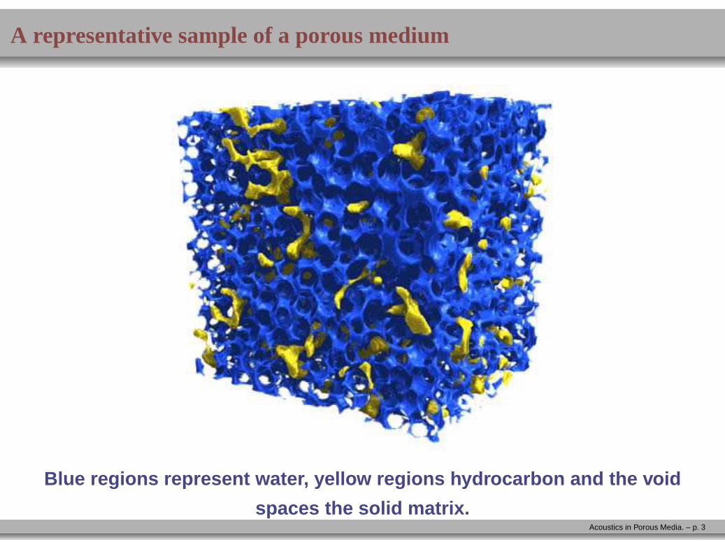
A representative sample of a porous medium

Blue regions represent water, yellow regions hydrocarbon a nd the void

spaces the solid matrix.Acoustics in Porous Media. – p. 3

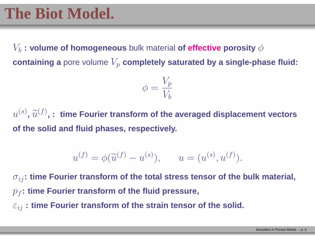
The Biot Model.

Vb : volume of homogeneous bulk material of effective porosity φ

containing a pore volume Vp completely saturated by a single-phase fluid:

φ =Vp

Vb

u(s), u(f), : time Fourier transform of the averaged displacement vect ors

of the solid and fluid phases, respectively.

u(f) = φ(u(f) − u(s)), u = (u(s), u(f)).

σij : time Fourier transform of the total stress tensor of the bul k material,

pf : time Fourier transform of the fluid pressure,

εij : time Fourier transform of the strain tensor of the solid.


Constitutive Relations.

σij(u) = 2µ εij(u(s)) + δij(λc∇ · u(s) + αKav ∇ · u(f)),

pf (u) = −αKav ∇ · u(s) − Kav ∇ · u(f),

where

α = 1 −Km

Ks

, Kav =

[α − φ

Ks

+φ

Kf

]−1

.

KG = Km + α2Kav λG = KG −2

3µ,

µ: shear modulus of the dry matrix,

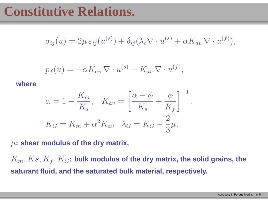
Km, Ks,Kf , KG: bulk modulus of the dry matrix, the solid grains, the

saturant fluid, and the saturated bulk material, respective ly.


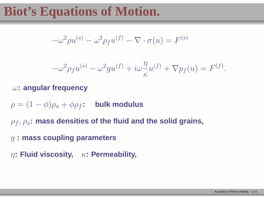
Biot’s Equations of Motion.

−ω2ρu(s) − ω2ρfu(f) −∇ · σ(u) = F (s)

−ω2ρfu(s) − ω2gu(f) + iω

η

κu(f) + ∇pf (u) = F (f).

ω: angular frequency

ρ = (1 − φ)ρs + φρf : bulk modulus

ρf , ρs: mass densities of the fluid and the solid grains,

g : mass coupling parameters

η: Fluid viscosity, κ: Permeability,


Plane Wave Analysis

In these type of media, two compressional waves ( P1, P2) and oneshear wave (or S)-wave) can propagate.

P1 and S waves: analogues of the classical fast waves propagatingin elastic or viscoelastic isotropic solids.

P2 wave: slow diffusion type wave in the low frequency range anda truly propagating mode in the ultrasonic range.

The P2 wave is due to the motions out of phase of the solid and fluidphases.

P2 waves are generated by conversion of the fast P1 and S waves atinterfaces within heterogeneous poroelastic materials, c ausingattenuation and dispersion on the fast modes.


A Variational Formulation. 2D Case.

Ω : rectangular domain , V = [H1(Ω)]2× H(div ; Ω).

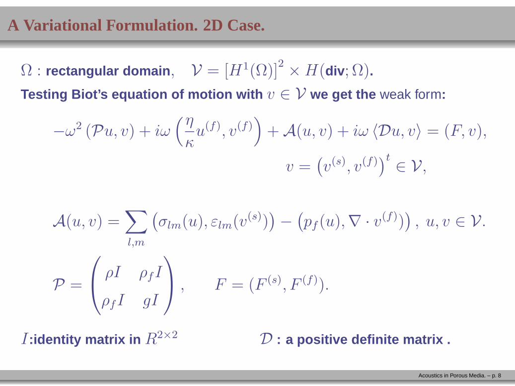
Testing Biot’s equation of motion with v ∈ V we get the weak form:

−ω2 (Pu, v) + iω(η

κu(f), v(f)

)+ A(u, v) + iω 〈Du, v〉 = (F, v),

v =(v(s), v(f)

)t∈ V,

A(u, v) =∑

l,m

(σlm(u), εlm(v(s))

)−

(pf (u),∇ · v(f))

), u, v ∈ V.

P =

ρI ρfI

ρfI gI

, F = (F (s), F (f)).

I :identity matrix in R2×2 D : a positive definite matrix .


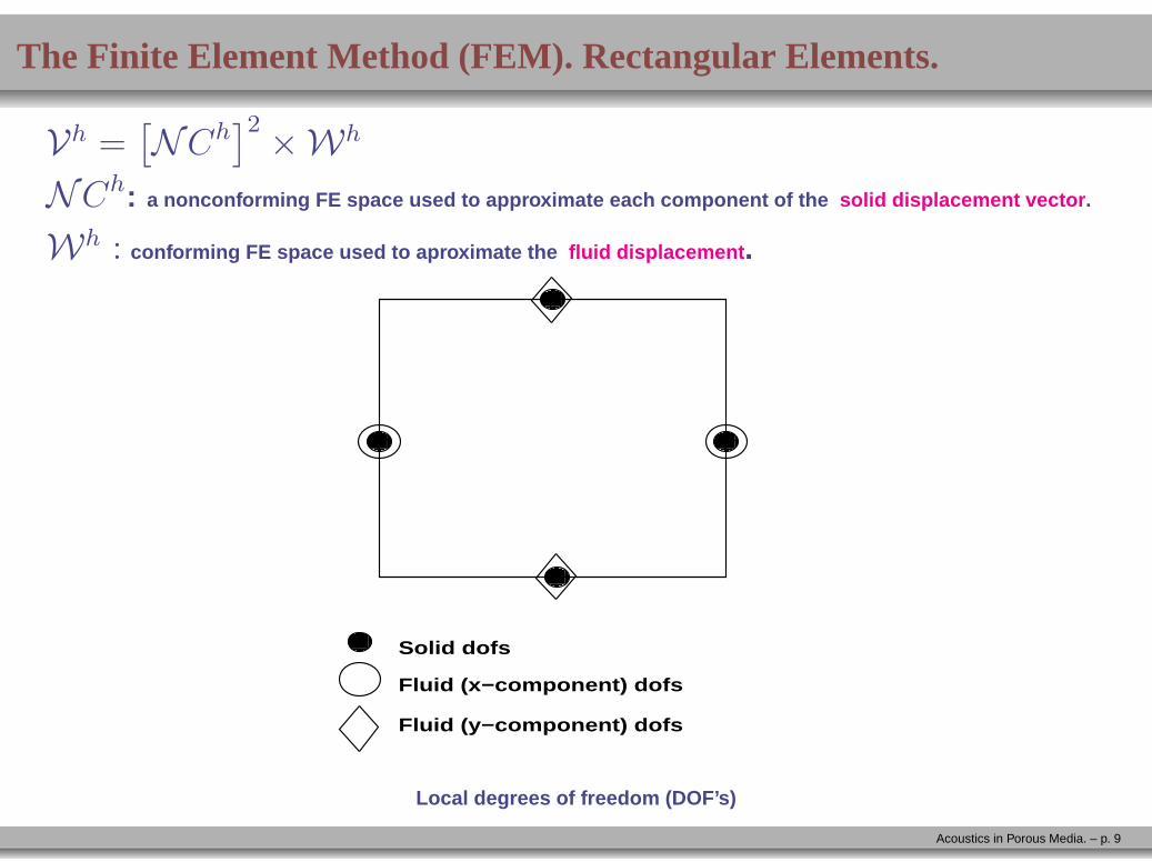
The Finite Element Method (FEM). Rectangular Elements.

Vh =[NCh

]2×Wh

NCh: a nonconforming FE space used to approximate each component of the solid displacement vector .

Wh : conforming FE space used to aproximate the fluid displacement .

Solid dofs

Fluid (x−component) dofs

Fluid (y−component) dofs

Local degrees of freedom (DOF’s)


Applications. The Mesoscopic Loss Mechanism. I

A major cause of seismic attenuation in porous media iswave-induced fluid flow , which occurs at mesoscopic scales.

A fast P1 wave induces a fluid-pressure difference atmesoscopic-scale inhomogeneities (larger than the pore si zebut smaller than the wavelength, typically tens of cen- time tres),generating fluid flow and slow (diffusion) P2 Biot waves

White (1975) was the first to show that mesoscopic loss can beobserved in the seismic range in a sandstone with partial gassaturation.

Next we show a numerical verification of the mesoscopic lossmechanism using the FEM.


Numerical Simulations to illustrate the mesoscopic loss mechanism.

The computational domain is a square of side length 800 m representing a

poroelastic rock alternately saturated with gas and water.

The perturbation F = (F (s), F (f)) is a compressional point source

applied to the matrix, located inside the region at (xs, ys) = (400 m, 4 m)

with (dominant) frequency 20 Hz.

Biot’s equations of motion were solved for 110 temporal freq uencies in

the interval (0, 60Hz) employing a FE domain decomposition iterative

procedure.

The domain was discretized into square cells of side length h = 40 cm.

The time domain solution was obtained performing an approxi mate

inverse Fourier transform.


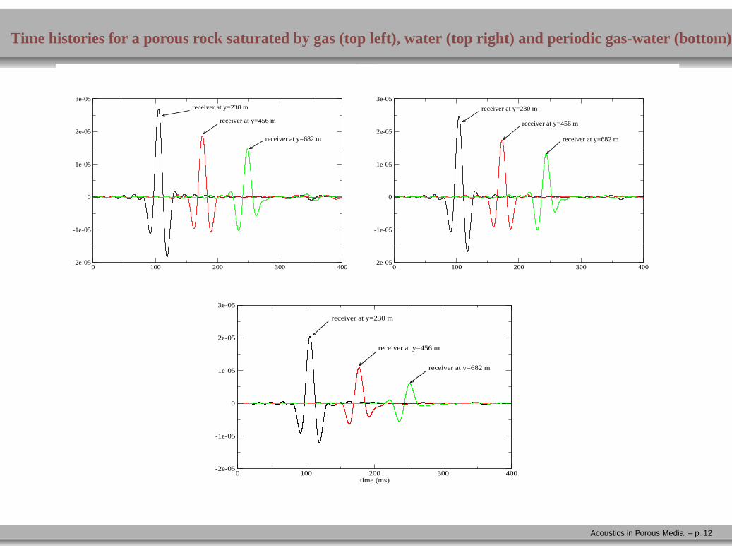
Time histories for a porous rock saturated by gas (top left),water (top right) and periodic gas-water (bottom)

0 100 200 300 400time (ms)

-2e-05

-1e-05

0

1e-05

2e-05

3e-05receiver at y=230 m

receiver at y=456 m

receiver at y=682 m

0 100 200 300 400time (ms)

-2e-05

-1e-05

0

1e-05

2e-05

3e-05

receiver at y=230 m

receiver at y=456 m

receiver at y=682 m

0 100 200 300 400time (ms)

-2e-05

-1e-05

0

1e-05

2e-05

3e-05

receiver at y=230 m

receiver at y=456 m

receiver at y=682 m


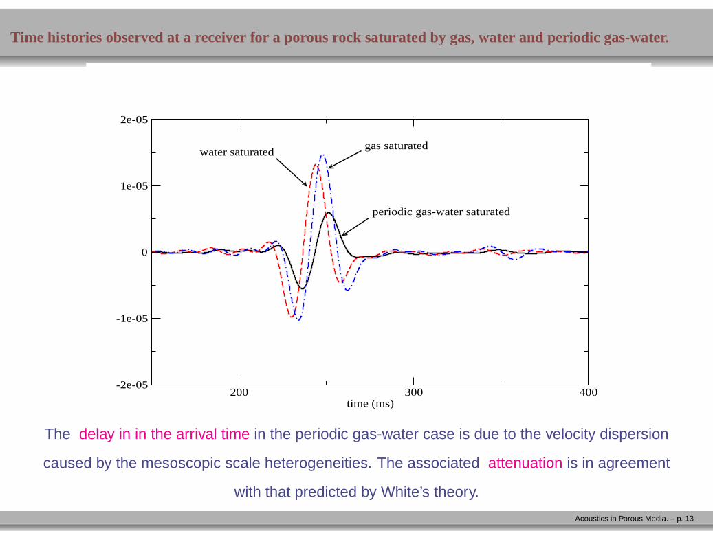
Time histories observed at a receiver for a porous rock saturated by gas, water and periodic gas-water.

200 300 400time (ms)

-2e-05

-1e-05

0

1e-05

2e-05

periodic gas-water saturated

gas saturatedwater saturated

The delay in in the arrival time in the periodic gas-water case is due to the velocity dispersion

caused by the mesoscopic scale heterogeneities. The associated attenuation is in agreement

with that predicted by White’s theory.


Extensions of Biot theory.

A porous medium saturated by immiscible fluids. The theory wa s

presented by Santos et al. (J. Acoust. Soc. Am., 1990a, b).

In these type of media, three compressional waves ( P1, P2, P3 waves)

and one shear wave ( S wave) can propagate.

A porous composite matrix saturated by a single-phase fluid. The

theory was developped by Leclaire et al. (J. Acoust. Soc. Am. , 1995)

for the uniform porosity case and then extended to the more re alistic

variable porosity case by Carcione et al. (J. Appl. Physics, 2003) and

Santos et a. (J. Acoust. Soc. Am., 2004).

In this case 3 compressional waves ( P1, P2, P3 waves) and 2 shear

waves (S1, S2 waves) can propagate. Observation of the slow waves

were presented in Leclaire et al. (J. Acoust. Soc. Am., 1995) .


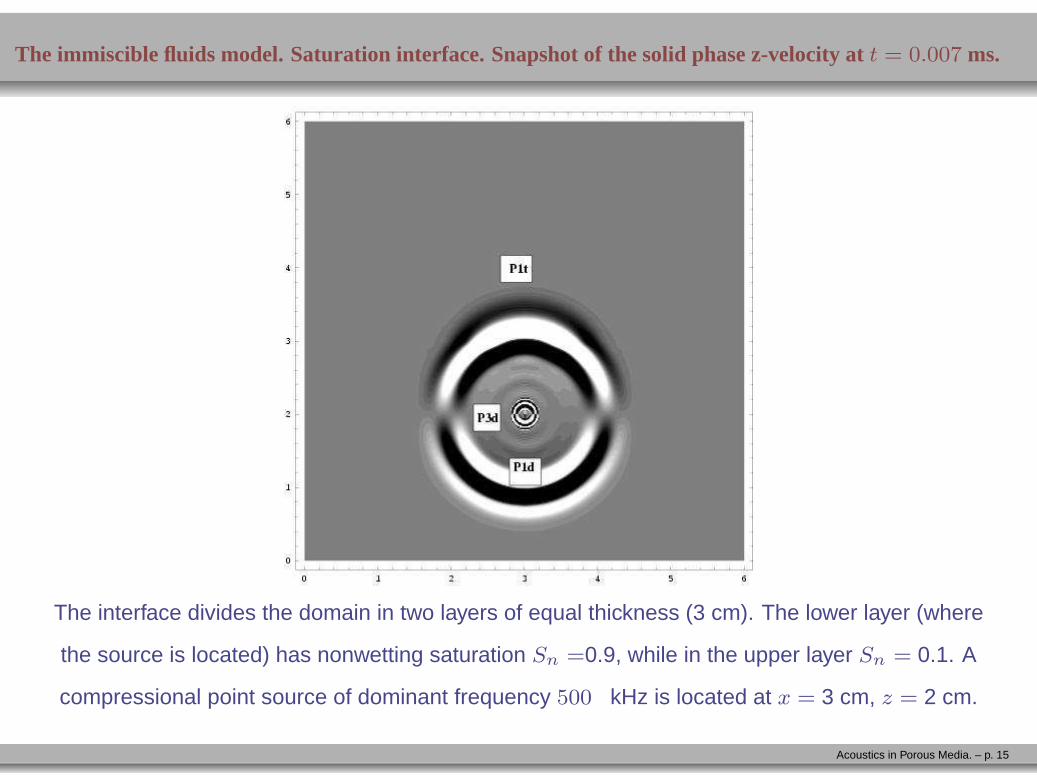
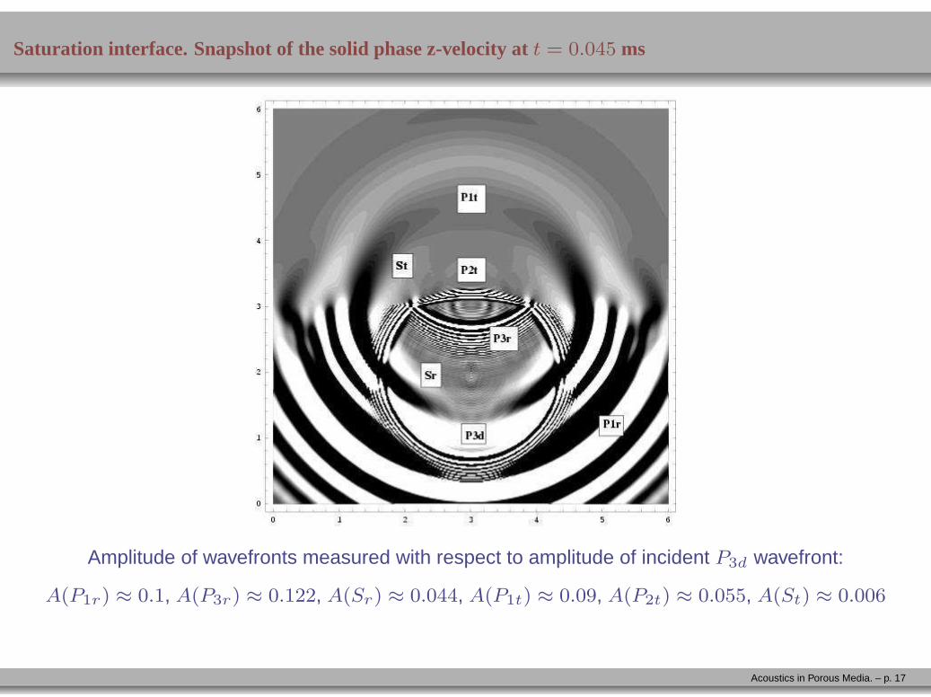
The immiscible fluids model. Saturation interface. Snapshot of the solid phase z-velocity att = 0.007 ms.

The interface divides the domain in two layers of equal thickness (3 cm). The lower layer (where

the source is located) has nonwetting saturation Sn =0.9, while in the upper layer Sn = 0.1. A

compressional point source of dominant frequency 500 kHz is located at x = 3 cm, z = 2 cm.


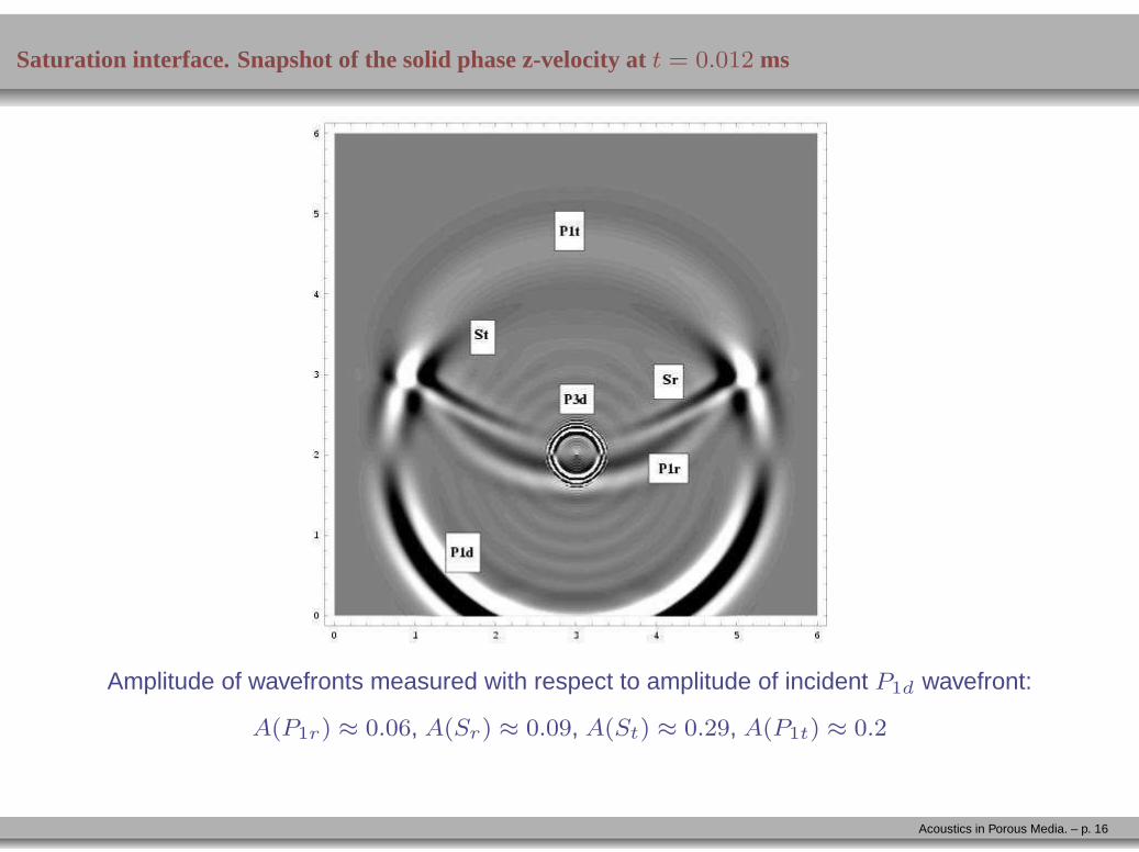
Saturation interface. Snapshot of the solid phase z-velocity at t = 0.012 ms

Amplitude of wavefronts measured with respect to amplitude of incident P1d wavefront:

A(P1r) ≈ 0.06, A(Sr) ≈ 0.09, A(St) ≈ 0.29, A(P1t) ≈ 0.2


Saturation interface. Snapshot of the solid phase z-velocity at t = 0.045 ms

Amplitude of wavefronts measured with respect to amplitude of incident P3d wavefront:

A(P1r) ≈ 0.1, A(P3r) ≈ 0.122, A(Sr) ≈ 0.044, A(P1t) ≈ 0.09, A(P2t) ≈ 0.055, A(St) ≈ 0.006


Patchy saturation map. White regions correspond to almost full gas saturation.

Macroscopic nonwetting saturation Sn = 0.1


Patchy saturation. Snapshot of the solid phase z-velocity at t = 0.007 ms

Irregular wavefronts are associated with compressional an d shear waves

generated at the gas patches. Thin wavefronts are associate d with slow

P2, P3 waves.Acoustics in Porous Media. – p. 19

Patchy saturation. Curl of the velocity of the solid phase att = 0.007 ms

Shear waves are generated at the gas-water interfaces by mod e

conversion.


The composite matrix model. Application to wave propagation in gas hydrate bearing sediments.

Gas hydrates (GH) are crystalline molecular complexes composed of

water and natural gas, mainly methane. They form under condi tions

of low temperature, high pressure and gas concentration and are

observed in permafrost regions and seaflor sediments along t he

continental margins.

GH are ice-like structures within the pore space that cause str ong

changes in the physical and mechanical properties of the roc k,

making possible to detect its presence using seismic data.

The interest in GH bearing sediments GH is mainly due to their

potential as future energy resources.


Wave Propagation in GH Bearing Sediments.

Borehole sonic log and cross-hole tomography data from the M allik

field (Mackenzie Delta, Canada), indicate that attenuation increases

with GH content .

Slow-waves energy conversions take place when a fast (class ical)

seismic wave strikes an heterogeneity within the GH bearing

sediments, generating slow compressional ( P2, P3) and shear ( S2)

waves.

These scattering-type effects can explain the observed lev els of

attenuation in GH-bearing sediments , which is tested using

numerical simulations.


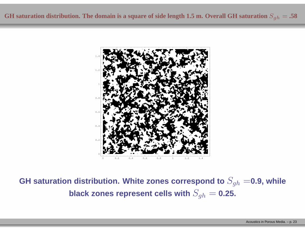
GH saturation distribution. The domain is a square of side length 1.5 m. Overall GH saturation Sgh = .58

0 0.2 0.4 0.6 0.8 1 1.2 1.4

0

0.2

0.4

0.6

0.8

1

1.2

1.4

GH saturation distribution. White zones correspond to Sgh =0.9, while

black zones represent cells with Sgh = 0.25.


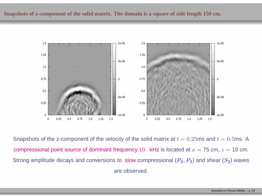
Snapshots of z-component of the solid matrix. The domain is asquare of side length 150 cm.

-1e-05

-5e-06

0

5e-06

1e-05

0 0.25 0.5 0.75 1.0 1.25 1.5

0

0.25

0.5

0.75

1.0

1.25

1.5

-1e-05

-5e-06

0

5e-06

1e-05

0 0.25 0.5 0.75 1.0 1.25 1.5

0

0.25

0.5

0.75

1.0

1.25

1.5

Snapshots of the z-component of the velocity of the solid matrix at t = 0.25ms and t = 0.5ms. A

compressional point source of dominant frequency 10 kHz is located at x = 75 cm, z = 10 cm.

Strong amplitude decays and conversions to slow compressional (P2, P3) and shear (S2) waves

are observed.


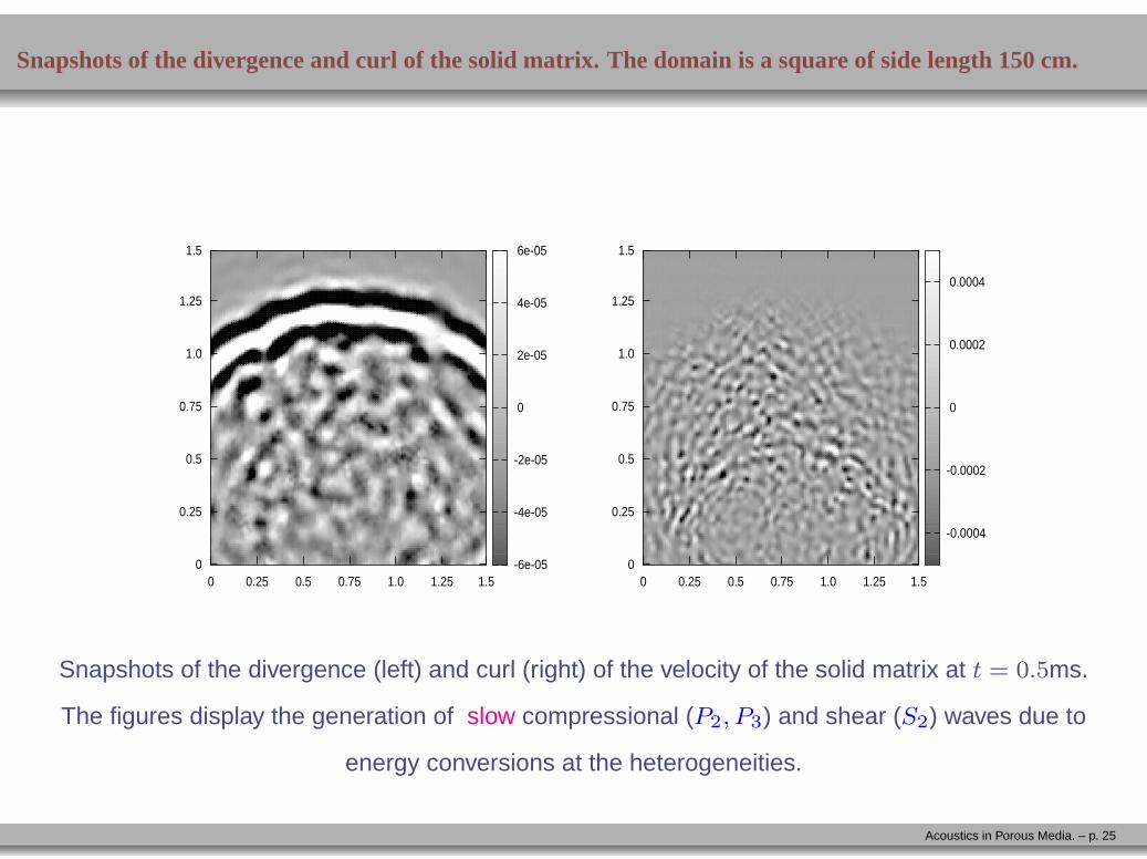
Snapshots of the divergence and curl of the solid matrix. Thedomain is a square of side length 150 cm.

-6e-05

-4e-05

-2e-05

0

2e-05

4e-05

6e-05

0 0.25 0.5 0.75 1.0 1.25 1.5

0

0.25

0.5

0.75

1.0

1.25

1.5

-0.0004

-0.0002

0

0.0002

0.0004

0 0.25 0.5 0.75 1.0 1.25 1.5

0

0.25

0.5

0.75

1.0

1.25

1.5

Snapshots of the divergence (left) and curl (right) of the velocity of the solid matrix at t = 0.5ms.

The figures display the generation of slow compressional (P2, P3) and shear (S2) waves due to

energy conversions at the heterogeneities.


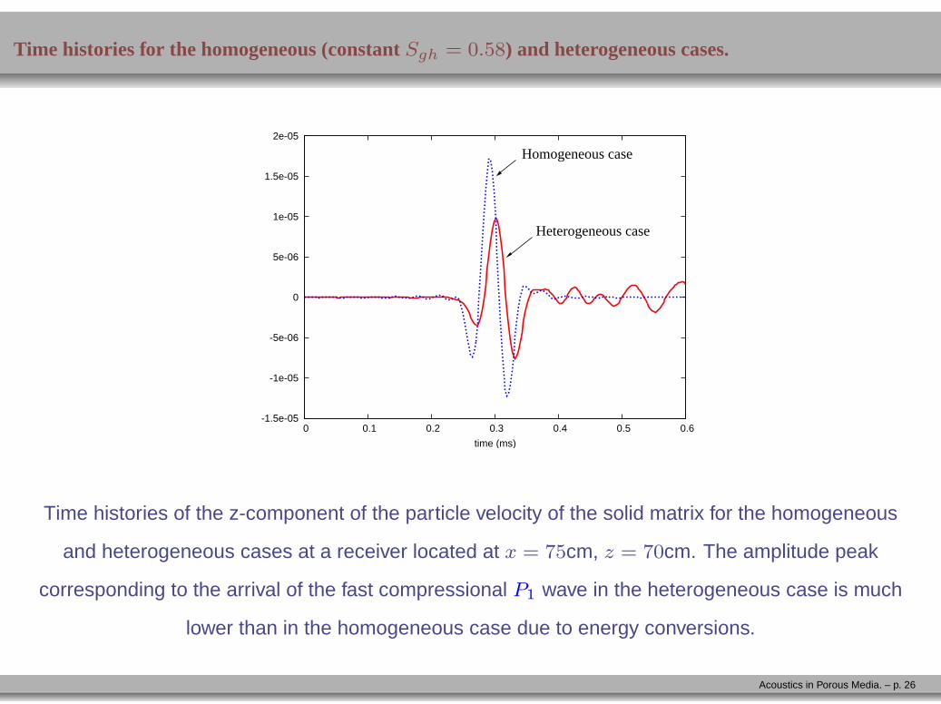
Time histories for the homogeneous (constantSgh = 0.58) and heterogeneous cases.

-1.5e-05

-1e-05

-5e-06

0

5e-06

1e-05

1.5e-05

2e-05

0 0.1 0.2 0.3 0.4 0.5 0.6

time (ms)

Homogeneous case

Heterogeneous case

Time histories of the z-component of the particle velocity of the solid matrix for the homogeneous

and heterogeneous cases at a receiver located at x = 75cm, z = 70cm. The amplitude peak

corresponding to the arrival of the fast compressional P1 wave in the heterogeneous case is much

lower than in the homogeneous case due to energy conversions.


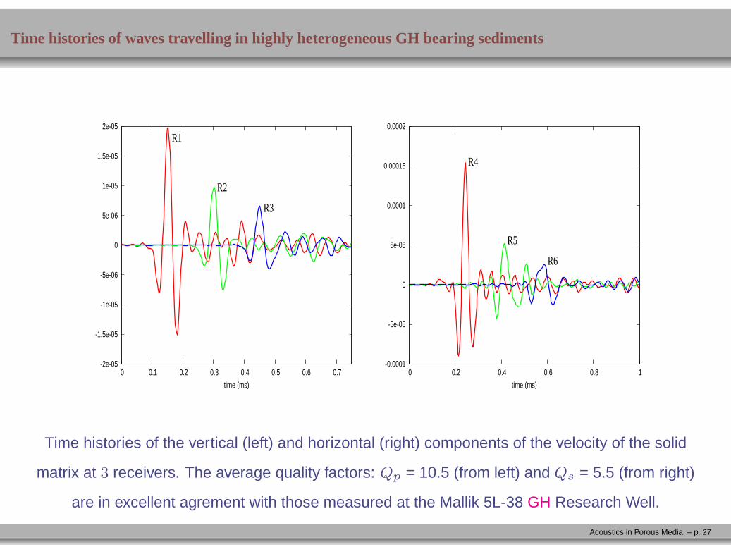
Time histories of waves travelling in highly heterogeneousGH bearing sediments

-2e-05

-1.5e-05

-1e-05

-5e-06

0

5e-06

1e-05

1.5e-05

2e-05

0 0.1 0.2 0.3 0.4 0.5 0.6 0.7

time (ms)

R1

R2

R3

-0.0001

-5e-05

0

5e-05

0.0001

0.00015

0.0002

0 0.2 0.4 0.6 0.8 1

time (ms)

R6

R5

R4

Time histories of the vertical (left) and horizontal (right) components of the velocity of the solid

matrix at 3 receivers. The average quality factors: Qp = 10.5 (from left) and Qs = 5.5 (from right)

are in excellent agrement with those measured at the Mallik 5L-38 GH Research Well.


Numerical simulations at the Mesoscale. I

Due to the extremely fine meshes needed to properly represent very

thin layers and other type of mesoscopic-scale heterogenei ties,

numerical simulations at the macroscale using Biot’s equat ions are

very expensive or even not feasible.

In the contex of Numerical Rock Physics , we use a numerical

upscaling procedure to determine the complex and frequency

dependent stiffness of an equivalent TIV medium at the macroscale

including the mesoscopic-scale effects.

The methodology is illustrated for the case of a fluid-satura ted

porous rock containing parallel fractures.


Fractured induced anisotropy in porous media. The Mesoscale. II

Seismic wave propagation through fractures is an important subject

in hydrocarbon exploration geophysics, mining and reservo ir

characterization and production.

Naturally fractured reservoirs have received interest in r ecent years,

since, generally, natural fractures control the permeabil ity of the

reservoir.

In geophysical prospecting and reservoir development, kno wledge of

fracture orientation, densities and sizes is essential sin ce these

factors control hydrocarbon production.

This is also important in CO 2 storage in geological formations to

monitor the injected plumes as faults and fractures are gene rated,

where CO 2 can leak to the surface.


Fractured induced anisotropy in porous media. The Mesoscale. III.

A planar fracture embedded in a fluid-saturated poroelastic

background is a particular case of the thin layer problem , when one

of the layers is very thin and compliant .

A dense set of horizontal fractures in a fluid-saturated poro elastic

medium behaves as a Transversely Isotropic Viscoelastic (TIV)

medium when the average fracture distance is much smaller than the

predominant wavelength of the traveling waves.

Wave anelasticity and anisotropy are significant in fractur ed

poroelastic rocks due to conversion of fast compressional w aves into

diffusion-type Biot slow waves.

This leads to frequency and angular variations of velocity a nd

attenuation of seismic waves.


The constitutive relations of a TIV media.

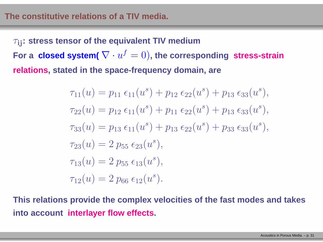
τij: stress tensor of the equivalent TIV medium

For a closed system( ∇ · uf = 0), the corresponding stress-strain

relations , stated in the space-frequency domain, are

τ11(u) = p11 ǫ11(us) + p12 ǫ22(u

s) + p13 ǫ33(us),

τ22(u) = p12 ǫ11(us) + p11 ǫ22(u

s) + p13 ǫ33(us),

τ33(u) = p13 ǫ11(us) + p13 ǫ22(u

s) + p33 ǫ33(us),

τ23(u) = 2 p55 ǫ23(us),

τ13(u) = 2 p55 ǫ13(us),

τ12(u) = 2 p66 ǫ12(us).

This relations provide the complex velocities of the fast mo des and takes

into account interlayer flow effects .


The harmonic experiments to determine the stiffness coeffic ients. I

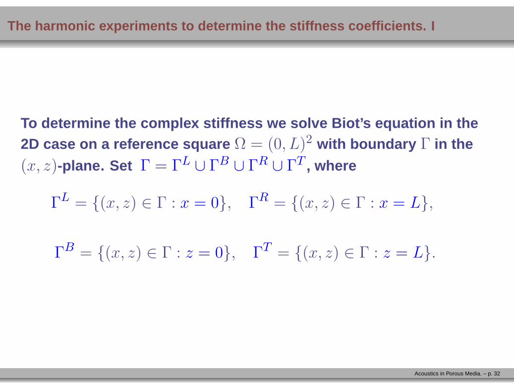
To determine the complex stiffness we solve Biot’s equation in the2D case on a reference square Ω = (0, L)2 with boundary Γ in the

(x, z)-plane. Set Γ = ΓL ∪ ΓB ∪ ΓR ∪ ΓT , where

ΓL = (x, z) ∈ Γ : x = 0, ΓR = (x, z) ∈ Γ : x = L,

ΓB = (x, z) ∈ Γ : z = 0, ΓT = (x, z) ∈ Γ : z = L.


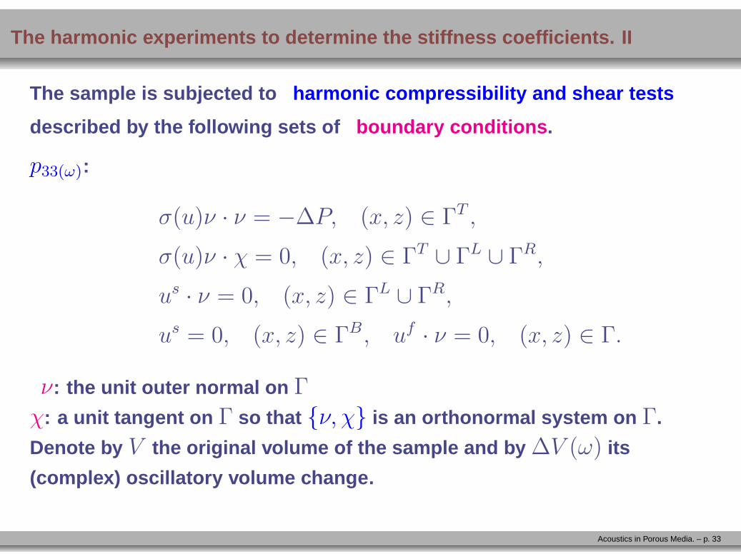
The harmonic experiments to determine the stiffness coeffic ients. II

The sample is subjected to harmonic compressibility and shear tests

described by the following sets of boundary conditions .

p33(ω):

σ(u)ν · ν = −∆P, (x, z) ∈ ΓT ,

σ(u)ν · χ = 0, (x, z) ∈ ΓT ∪ ΓL ∪ ΓR,

us · ν = 0, (x, z) ∈ ΓL ∪ ΓR,

us = 0, (x, z) ∈ ΓB, uf · ν = 0, (x, z) ∈ Γ.

ν: the unit outer normal on Γ

χ: a unit tangent on Γ so that ν, χ is an orthonormal system on Γ.

Denote by V the original volume of the sample and by ∆V (ω) its

(complex) oscillatory volume change.


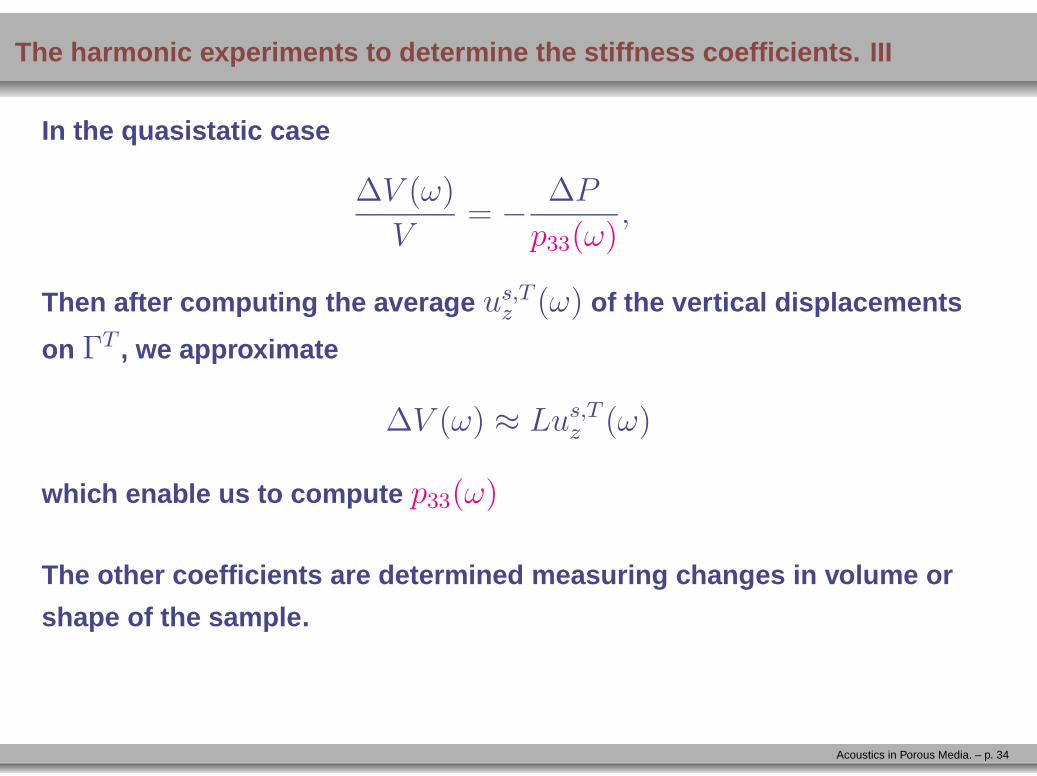
The harmonic experiments to determine the stiffness coeffic ients. III

In the quasistatic case

∆V (ω)

V= −

∆P

p33(ω),

Then after computing the average us,Tz (ω) of the vertical displacements

on ΓT , we approximate

∆V (ω) ≈ Lus,Tz (ω)

which enable us to compute p33(ω)

The other coefficients are determined measuring changes in v olume or

shape of the sample.


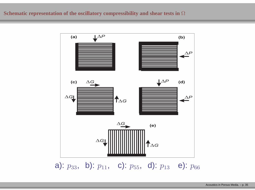
Schematic representation of the oscillatory compressibility and shear tests inΩ

DP

DG DP

DP

(a) (b)

(c) (d)

DG

DG

(e)

DG

DG

DG

DP

a): p33, b): p11, c): p55, d): p13 e): p66


Examples . I

A set of numerical examples consider the following cases for asquare poroelastic sample of 160 cm side length and 10 period s of 1cm fracture, 15 cm background:

Case 1: A brine-saturated sample with fractures.

Case 2: A brine-CO 2 patchy saturated sample without fractures.

Case 3: A brine-CO 2 patchy saturated sample with fractures.

Case 4: A brine saturated sample with a fractal frame andfractures.


Examples . II

The discrete BVP’s to determine the complex stiffnesses pIJ (ω)

were solved for 30 frequencies using a public domain sparsematrix solver package.

Using relations not included for brevity, the pIJ (ω)’s determinein turn the energy velocities and dissipation coefficients s hownin the next figures.


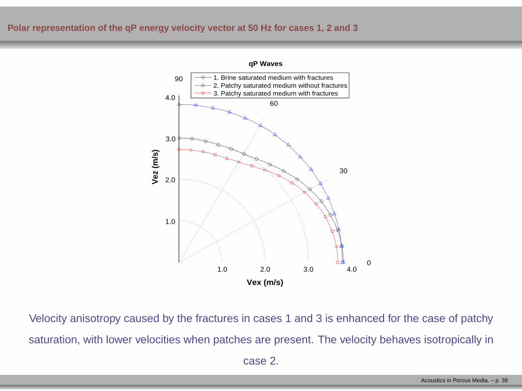
Polar representation of the qP energy velocity vector at 50 H z for cases 1, 2 and 3

1.0

2.0

3.0

4.0

30

60

90

0

qP Waves

Vex (m/s)

Vez

(m/s

)

1. Brine saturated medium with fractures2. Patchy saturated medium without fractures 3. Patchy saturated medium with fractures

1.0 2.0 3.0 4.0

Velocity anisotropy caused by the fractures in cases 1 and 3 is enhanced for the case of patchy

saturation, with lower velocities when patches are present. The velocity behaves isotropically in

case 2.


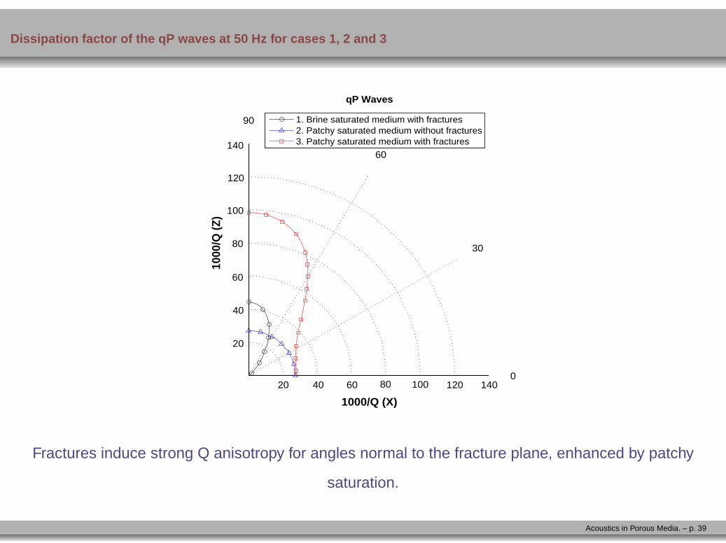
Dissipation factor of the qP waves at 50 Hz for cases 1, 2 and 3

20

40

60

80

100

120

140

30

60

90

0

qP Waves

1000/Q (X)

1000

/Q (Z

)


10080604020 120 140

Fractures induce strong Q anisotropy for angles normal to the fracture plane, enhanced by patchy

saturation.


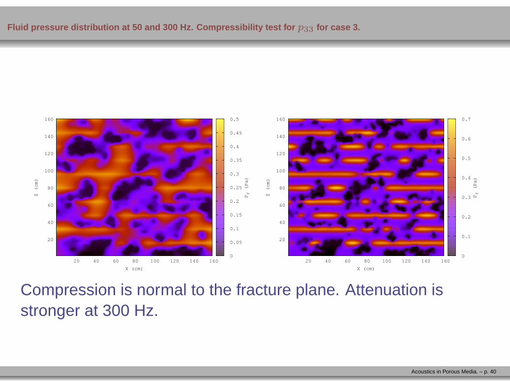
Fluid pressure distribution at 50 and 300 Hz. Compressibili ty test for p33 for case 3.

20

40

60

80

100

120

140

160

20 40 60 80 100 120 140 160

Z (cm)

X (cm)

’Salida_presion_p33’

0

0.05

0.1

0.15

0.2

0.25

0.3

0.35

0.4

0.45

0.5

Pf (Pa)

20

40

60

80

100

120

140

160

20 40 60 80 100 120 140 160

Z (cm)

X (cm)

’Salida_presion_p33’

0

0.1

0.2

0.3

0.4

0.5

0.6

0.7

Pf (Pa)

Compression is normal to the fracture plane. Attenuation isstronger at 300 Hz.


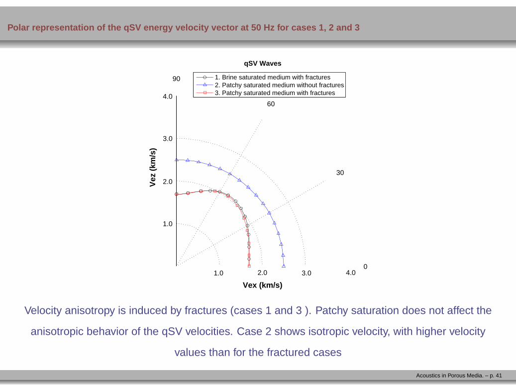
Polar representation of the qSV energy velocity vector at 50 Hz for cases 1, 2 and 3

1.0

2.0

3.0

4.0

30

60

90

0

qSV Waves

Vex (km/s)

Vez

(km

/s)


1.0 2.0 3.0 4.0

Velocity anisotropy is induced by fractures (cases 1 and 3 ). Patchy saturation does not affect the

anisotropic behavior of the qSV velocities. Case 2 shows isotropic velocity, with higher velocity

values than for the fractured cases


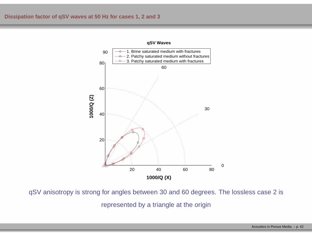
Dissipation factor of qSV waves at 50 Hz for cases 1, 2 and 3

20

40

60

80

30

60

90

0

qSV Waves

1000/Q (X)

1000

/Q (Z

)


60 8020 40

qSV anisotropy is strong for angles between 30 and 60 degrees. The lossless case 2 is

represented by a triangle at the origin


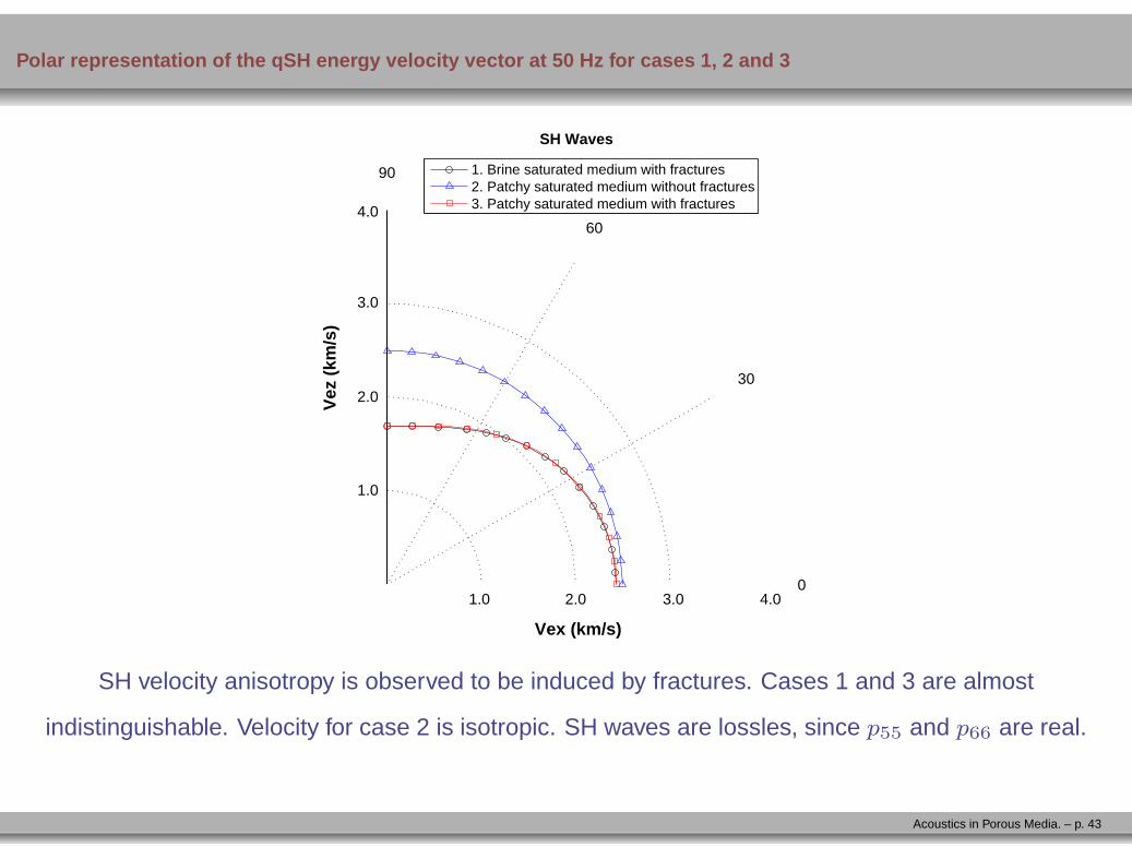
Polar representation of the qSH energy velocity vector at 50 Hz for cases 1, 2 and 3

1.0

2.0

3.0

4.0

30

60

90

0

SH Waves

Vex (km/s)

Vez

(km

/s)


1.0 2.0 3.0 4.0

SH velocity anisotropy is observed to be induced by fractures. Cases 1 and 3 are almost

indistinguishable. Velocity for case 2 is isotropic. SH waves are lossles, since p55 and p66 are real.


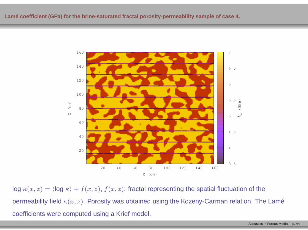
Lame coefficient (GPa) for the brine-saturated fractal porosit y-permeability sample of case 4.

20

40

60

80

100

120

140

160

20 40 60 80 100 120 140 160

Z (cm)

X (cm)

’lambda_global_gnu_2.dat’

3.5

4

4.5

5

5.5

6

6.5

7

λ G (GPa)

log κ(x, z) = 〈log κ〉 + f(x, z), f(x, z): fractal representing the spatial fluctuation of the

permeability field κ(x, z). Porosity was obtained using the Kozeny-Carman relation. The Lamé

coefficients were computed using a Krief model.Acoustics in Porous Media. – p. 44

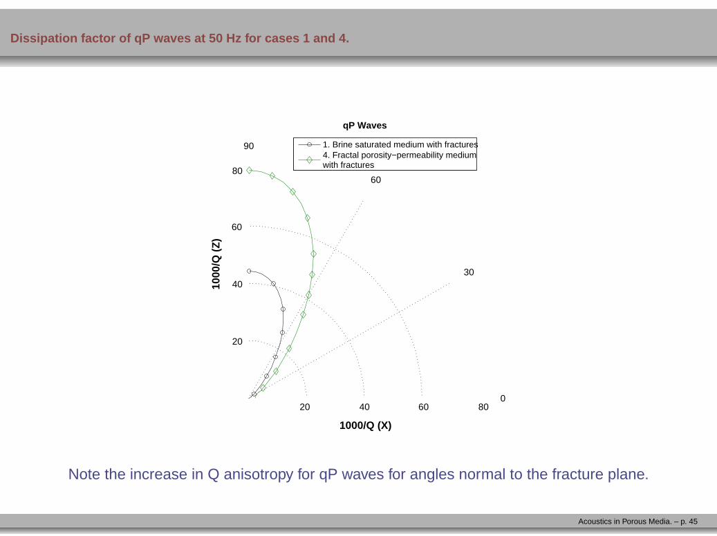
Dissipation factor of qP waves at 50 Hz for cases 1 and 4.

20

40

60

80

30

60

90

0

qP Waves

1000/Q (X)

1000

/Q (

Z)

1. Brine saturated medium with fractures4. Fractal porosity−permeability mediumwith fractures

20 60 8040

Note the increase in Q anisotropy for qP waves for angles normal to the fracture plane.


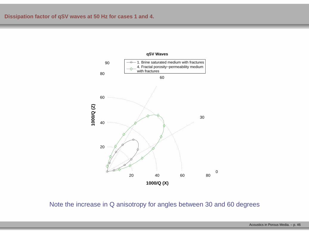
Dissipation factor of qSV waves at 50 Hz for cases 1 and 4.

20

40

60

80

30

60

90

0

qSV Waves

1000/Q (X)

1000

/Q (

Z)

1. Brine saturated medium with fractures 4. Fractal porosity−permeability mediumwith fractures

20 60 8040

Note the increase in Q anisotropy for angles between 30 and 60 degrees


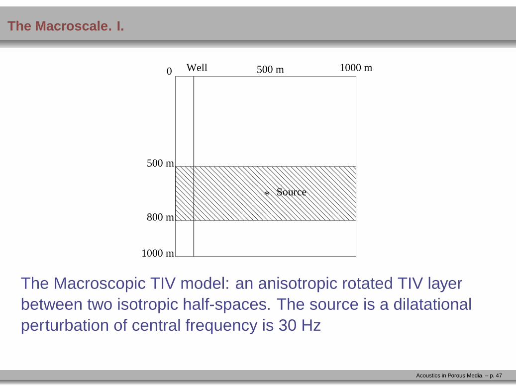
The Macroscale. I.

*

0 1000 m

1000 m

800 m

500 m

Source

Well 500 m

The Macroscopic TIV model: an anisotropic rotated TIV layerbetween two isotropic half-spaces. The source is a dilatationalperturbation of central frequency is 30 Hz


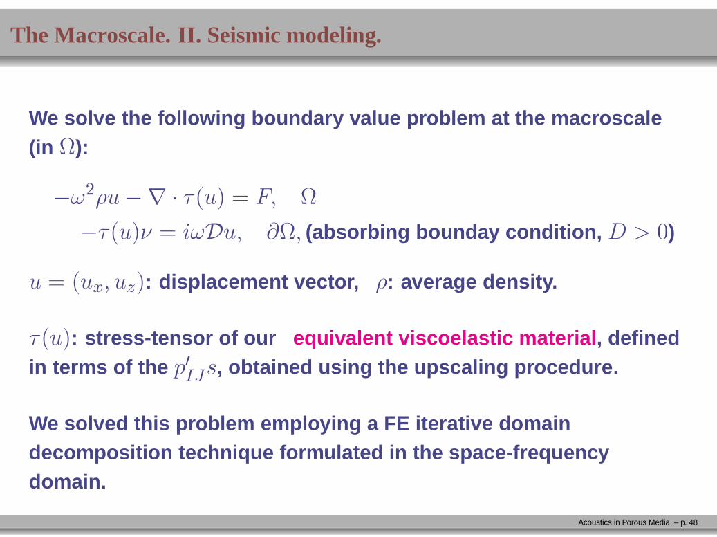
The Macroscale. II. Seismic modeling.

We solve the following boundary value problem at the macrosc ale(in Ω):

−ω2ρu −∇ · τ(u) = F, Ω

−τ(u)ν = iωDu, ∂Ω, (absorbing bounday condition, D > 0)

u = (ux, uz): displacement vector, ρ: average density.

τ(u): stress-tensor of our equivalent viscoelastic material , definedin terms of the p′IJs, obtained using the upscaling procedure.

We solved this problem employing a FE iterative domaindecomposition technique formulated in the space-frequenc ydomain.


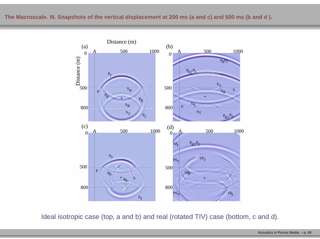
The Macroscale. III. Snapshots of the vertical displacemen t at 200 ms (a and c) and 500 ms (b and d ).

*

S

S

S

S

S

SR

R

T

T

P

P

PRPT

R2

R2

P

P

T

T

*

P

P

P

T

T

SP

PR

R *

PS

PS

T

T

PR2 TP

S

SPT

SPT

PT

SPR

*

P

P

PP

P

T

T

RR

S

S

SR

R

T

A A

A A

(a)

(d)

(b)

(c)

Distance (m)

Dis

tanc

e (m

)

0

0

0

0

500

500

500

500

500 500

500 500

800

800 800

800

1000 1000

1000 1000

Ideal isotropic case (top, a and b) and real (rotated TIV) case (bottom, c and d).


ConclusionsNumerical simulation is a useful tool in hydrocarbon explor ation

geophysics, mining and reservoir characterization and pro duction.

The FEM allows to analyze and represent mesoscopic scale

heterogeneities in the solid frame and saturant fluids, frac tures and

craks affecting observations at the macroscale.

Wave propagation at the macroscale can be efficiently perfor med

employing the FEM combined with iterative domain decomposi tion

techniques formulated in the space-frequency domain.

The ideas presented here to model acoustics of porous media c an be

extended to other fields, like ultrasound testing of quality of foods,

groundwater flow and contamination among others.

Thanks for your attention !!!!!.


Date post:	10-May-2018
Category:	Documents
Upload:	vuongdat
View:	216 times
Download:	0 times

Acoustics in Porous Media. - Purdue Universitysantos/research/corbino_2013/corbino.pdfAcoustics in...

Documents