Acousto-optical interaction and its
advanced applications
By:
Phys. Adán Omar Arellanes Bernabe
A dissertation Submitted to the program in Optics.
Optics department.
In partial fulfillment of the requirements for the degree of
MASTER IN SCIENCES WITH SPECIALITY
OF OPTICS
At:
National Institute for Astrophysics,
Optics, and Electronics.
August 2013
Tonantzintla, Puebla.
Advisor:
Dr. Alexander S. Shcherbakov
INAOE Researcher
Optics Department
©INAOE 2013
All rights reserved
The author hereby grants to INAOE permission
to reproduce and to distribute copies of this
thesis in whole or in part.
1
Contents 1. Acousto-Optics 15
1.1. Light Propagation in Anisotropic Media 15
1.1.1. Index Ellipsoid and Surfaces. 15
1.1.2. Crystals; Optically Isotropic, Uniaxial and Biaxial 17
1.2. Ultrasound Propagation in Anisotropic Media 18
1.2.1. Pure Longitudinal Waves 19
1.2.2. Pure Shear Waves 20
1.3. Acousto-Optical Interactions 20
1.3.1. Wave Vector Diagrams; Normal and Anomalous Light
Scattering 21
1.3.2. Collinear Interaction 23
1.3.3. Non-Collinear Interaction 23
1.4. The Formal Approach (Differential Equation Method) 24
1.5. Applications of Modulation, Filtering and Deflection 27
1.6. Acousto-Optic Properties of Materials 29
1.7. Formulation of Problems 33
2. Acousto-Optical Version of Optical Spectrometer for Guillermo
Haro Observatory 35
2.1. Introduction 35
2.2. Guillermo Haro Observatory Spectrograph Performances 38
2.2.1. Calculations for the Spectral Resolution 40
2.3. Acousto-Optical Cell 41
2.3.1. The nature of Acousto-optical dynamic diffraction grating 41
2.3.2. Requirements and Design 43
2.3.3. Material Selection 43
2.4. Diffraction of the light beam of finite width by a harmonic acoustic
wave at low acousto-optic efficiency 46
2.5. Conclusions 50
3. Transmission Function of Advanced Collinear Acousto-Optical
Filter 51
3.1. Theory and Operation 51
3.2. Three Wave Collinear Interaction 52
3.3. Efficiency of Collinear Interaction in CaMoO4 54
3.4. Resolution of CaMoO4 Filter 57
3.4.1. Traditional Approach 57
3.4.2. Loss-Less Medium Case 58
3.5. Some Estimations For The CaMoO4 AOTF 62
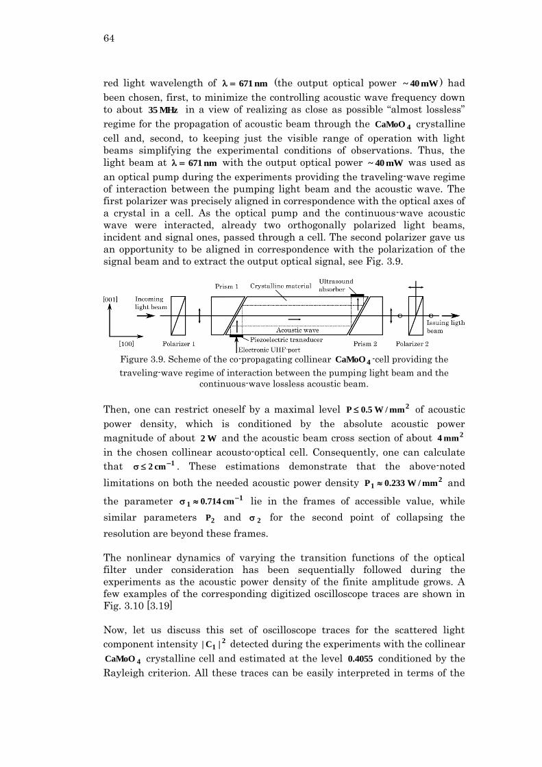
3.6. Scheme for the experiments with a CaMoO4 cell 63
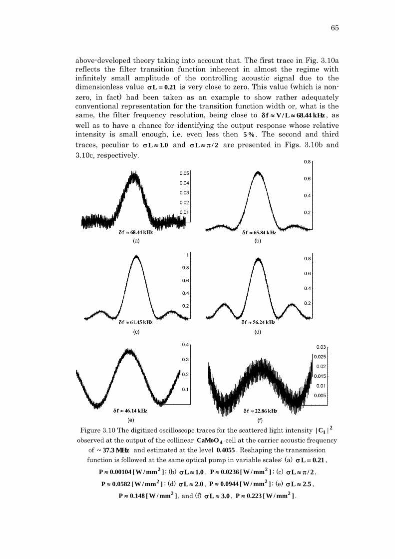
3.7. Conclusions 66
2
4. Acousto-Optical Triple Product Processor for Astrophysical
Applications 67
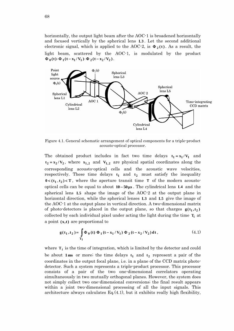
4.1. Introduction 67
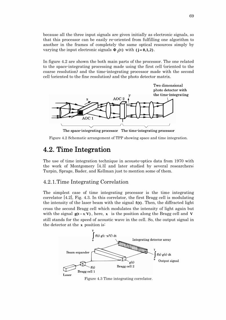
4.2. Time Integration 69
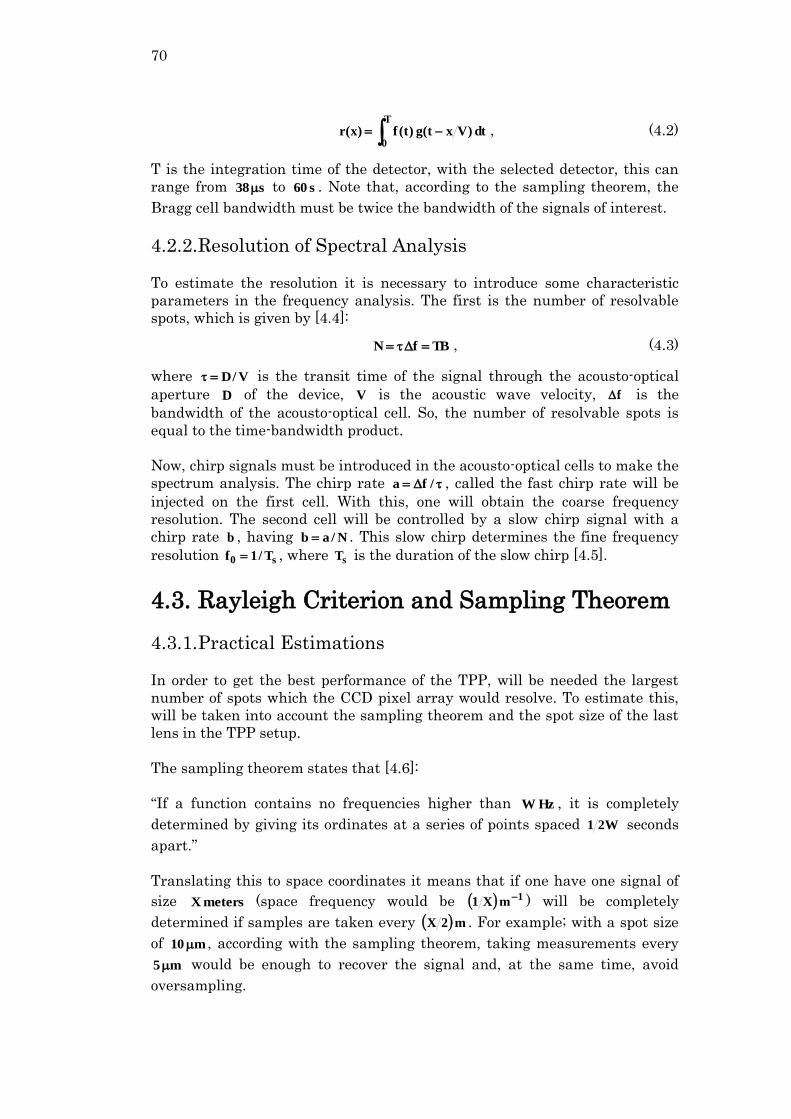
4.2.1. Time Integrating Correlation 69
4.2.2. Resolution of Spectral Analysis 70
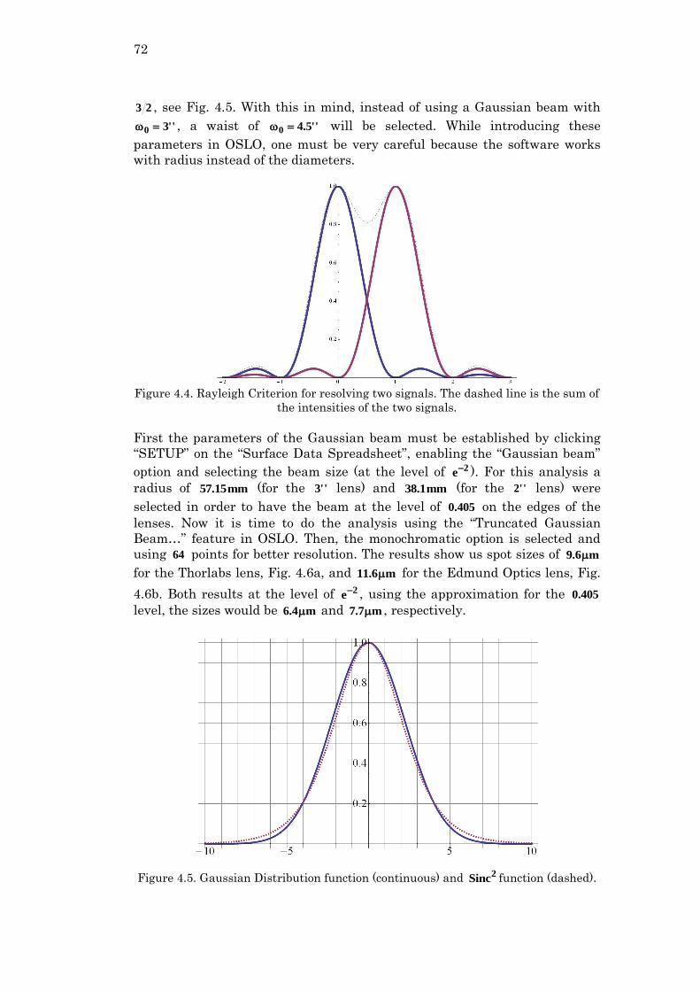
4.3. Rayleigh Criterion and Sampling Theorem 70
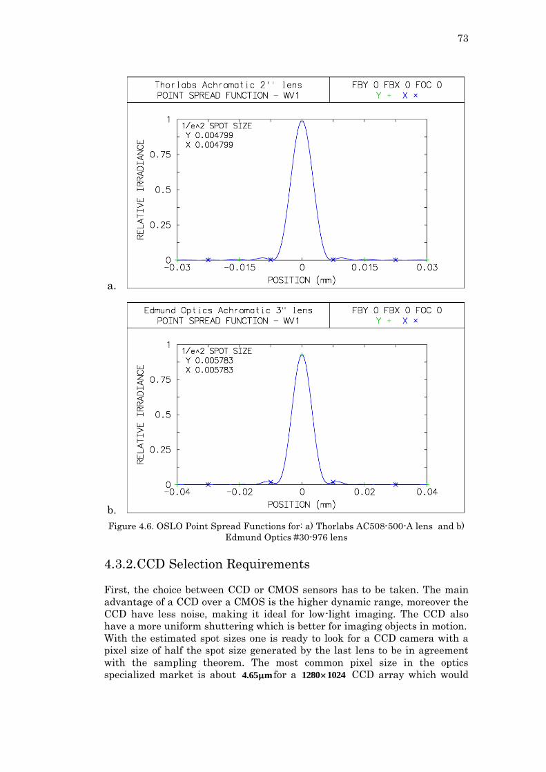
4.3.1. Practical Estimations 70
4.3.2. CCD Selection Requirements 73
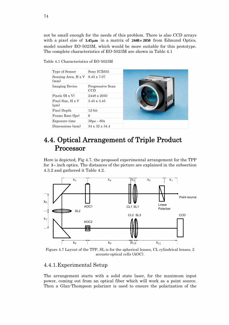
4.4. Optical Arrangement of Triple Product Processor 74
4.4.1. Experimental Setup 74
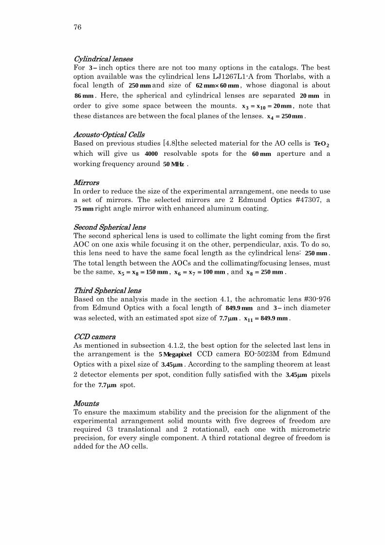
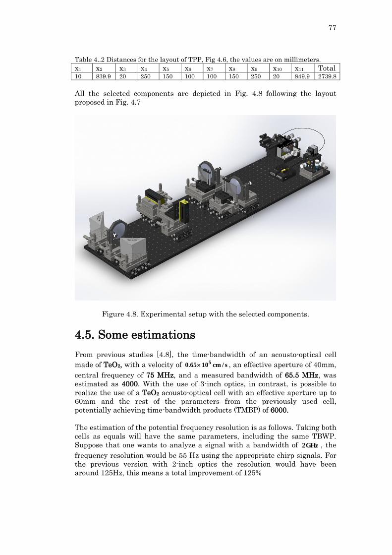
4.4.2. Components Selection 75
4.5. Some Estimations 77
4.6. Conclusions 78
5. General Conclusions 79
Future Work 81
Bibliography 83
Statements 87
5
Acknowledgements
I thank to all the Mexican people who, through CONACyT, makes possible all
the scientific development, including this thesis, in our country
I thank my advisor Dr. Alexander Shcherbakov for sharing all his experience
and knowledge, both scientific and personal.
Thanks to the INAOE for giving me all the knowledge to makes this work
possible.
Thanks to my co-authors Dr. Vahram Chavushyan and Dr. Sergey A. Nemov.
Thanks to my examiners Dr. David Sánchez de la Llave and Dr. Mauro
Sánchez Sánchez for their help and support.
Thanks to all my professors and specially Dr. Ponciano Rodriguez, Dr. Victor
Arrizon, Dr. Eugene Kuzin, Dr. Baldemar Ibarra, Dr. Sabino Chavez, and Dr.
Nikolai Korneev.
Also thanks to my colleagues and friends Gabriel Mellado, César Camacho,
Josué Peralta, Noemí Sánchez, Ana V. Hanessian, Fabián Villa, Mayra
Vargas, and Jesús Arriaga for all their support and company during my
studies.
Special thanks to my parents Adán Arellanes and Noemí Bernabe, and to my
sisters Diana, Patricia and Julia for their love and support.
7
Abstract
In this this work, the acousto-optical interaction is studied. Since its
inception, in 1922, it has been widely studied and applied. Here, the
development of three advanced application of this branch of physics is
considered.
First, is analyzed the potential use of an acousto-optical cell for be included as
a dynamic diffraction grating, in order to improve in many ways the actual
static gratings used, in the Guillermo Haro astrophysical observatory. For
this, it was necessary to estimate the performance of several acousto-optical
materials available today.
Second, a specific mechanism of the acousto-optical nonlinearity is studied to
regulate the performance of the collinear acousto-optical filter. The theory of
this phenomenon is analyzed and confirmed experimentally using and
advanced filter based on calcium molybdate ( 4CaMoO ) single-crystal. The
transmission function of electronically tunable filter exhibits a dependence on
the applied acoustic power density, and as a result, it is possible to squeeze
the transmission function at the cost of decreasing the device efficiency
partially.
And at final, the triple product processor is studied for its potential
application in spectroscopy designed for 3-inch optics and analyzing all the
materials needed for its realization. The need to use 3-inch optics is mainly
oriented to exploit an acousto-optical cells with large aperture windows to get
a large time-bandwidth product.
9
Resumen
En este trabajo se estudia la interacción acusto-óptica. Desde sus comienzos
en 1922 ha sido estudiada y aplicada ampliamente . Aquí están desarrolladas
tres aplicaciones avanzadas de esta rama de la física.
Primero, se analiza el uso potencial de una celda acusto-óptica para ser
incluida como una rejilla de difracción dinámica, con el fin de mejorar en
varios aspectos las rejillas que se usan actualmente en el observatorio
astrofísico Guillermo Haro en Cananea. Para esto fue necesario estimar el
desempeño de varios materiales acusto-ópticos disponibles en la actualidad.
Segundo, un mecanismo específico de la nolinealidad acusto-óptica es
estudiado para regular el desempeño de un filtro acusto-óptico colineal. La
teoría de este fenómeno es analizada y posteriormente confirmada
experimentalmente usando un filtro basado en un solo cristal de molibdato de
calcio ( 4CaMoO ). La función de transmisión del filtro sintonizable
electrónicamente muestra una dependencia en la densidad de potencia
acústica aplicada, y como resultado, es posible estrechar la función de
transmisión con la desventaja de disminuir parcialmente la eficiencia del
aparato.
Y por último se estudia un procesador de triple producto para su potencial
aplicación en espectroscopía, diseñado para un arreglo óptico de 3 pulgadas,
analizando los materiales necesarios para su realización. La necesidad de
usar el arreglo óptico de 3 pulgadas está principalmente orientado para
explotar una celda acusto-óptica con una larga ventana de apertura para
obtener un producto tiempo-ancho de banda grande.
11
Introduction
The acousto-optics is a branch of physics which joints the light phenomena
with the sound and ultrasound phenomena. The study of the interaction
between light and acoustic waves was first predicted by Brillouin in 1922 and
later, this idea was refined by Debye and Sears in 1932, and by Lucas and
Biquard. It continued with the investigations of Raman and Nath between
1935 and 1936. A heuristic physical approach was later proposed by Van
Cittert in 1937 and many more contributions were made in the theoretical
explanation of the phenomenon by many authors. Later, with the invention of
the laser in 1960, a new need for controlling the light was born and more
developments were made in acousto-optical applications and theory as well.
From deflection, filtering, and frequency shifting to parallel optical processing
for the study of signals, the acousto-optics has never stopped in its
development and has been used for several important experiments, for
example, the first Bose-Einstein condensate in 1995. It has also been widely
applied for spectroscopy in astrophysics, in filtering and acousto-optical
signal processing.
13
Preface
The study of acousto-optical interaction is widely discussed within this thesis.
Also, the development of new applications using this discipline is analyzed.
The main motivation for this matter is its use in astrophysical spectroscopy
but it is not limited to this area.
The first chapter is a very extensive introduction to acousto-optics, explaining
the nature of acoustical and optical waves in order to establish the basic
knowledge to understand the interaction between these two physical
phenomena. Some concepts of the propagation of these waves in a medium
are also explained.
In chapter number two, the design of a novel acousto-optical spectrometer for
the Guillermo Haro astrophysical observatory is discussed. The analysis for
the design of an acousto-optical cell for this spectrometer is also considered
and some estimations of its potential performance were made.
In the third chapter a specific mechanism in the non-linear regime of acousto-
optical interaction is discussed for its use in a collinear acousto-optical
tunable filter to control its transmission function with the use of acoustic
waves of finite amplitude.
The chapter four is directed to the analysis of the potential improvement of a
triple product processor using 3-inch optics components in order to exploit the
advantages for the time and space integration combined.
In the chapter five, the general conclusions of this thesis are presented.
Finally, some future work, related to the work developed in this thesis, is
presented.
15
Chapter 1
Acousto-Optics
In this chapter, the basic theory of the acousto-optical interaction and
generally some of the most used applications are presented [1.1] in order to
set up the knowledge for the more recent and advanced applications. To
understand this better, first is explained the behavior of the light in
anisotropic media, then the propagation of sound in some medium and finally
the interaction of these 2 phenomena.
1.1. Light Propagation in Anisotropic Media
The study of the propagation of light could be divided in two cases: isotropic
and anisotropic. In an isotropic media the induced polarization is always
parallel to the electric field and it is proportional to the susceptibility and this
relation is independent to the direction of the applied field. It becomes more
interesting for anisotropic media, where depending on the direction of the
light in the media and its state of polarization, the induced polarization
would change.
1.1.1. Index Ellipsoid and Surfaces.
Two different concepts must be introduced, which will allow the work
mathematically and help visualize the differences between each type of
crystals that will be used. In one hand it is the index ellipsoid which is
defined as [1.2]
1zyx
zz
2
yy
2
xx
2
, (1.1)
where ii are the components of the main diagonal in the dielectric tensor ,
and knowing that
n (1.2)
16
n is the refractive index and the magnetic permeability which is effectively
unity for all the materials are concerned for this thesis. Now it is possible to
rewrite (1.1) into
1n
z
n
y
n
x
2z
2
2y
2
2x
2
. (1.3)
As an example, let oyx nnn , ez nn , and let eo nn so Eq.(1.3) becomes
1n
z
n
yx
2e
2
2o
22
, (1.4)
with this spheroid in mind, consider the wave vector k
in the direction of an
arbitrary angle to the z axis, then any plane that touches the origin and
that is perpendicular to this wave vector will intersect the spheroid in an
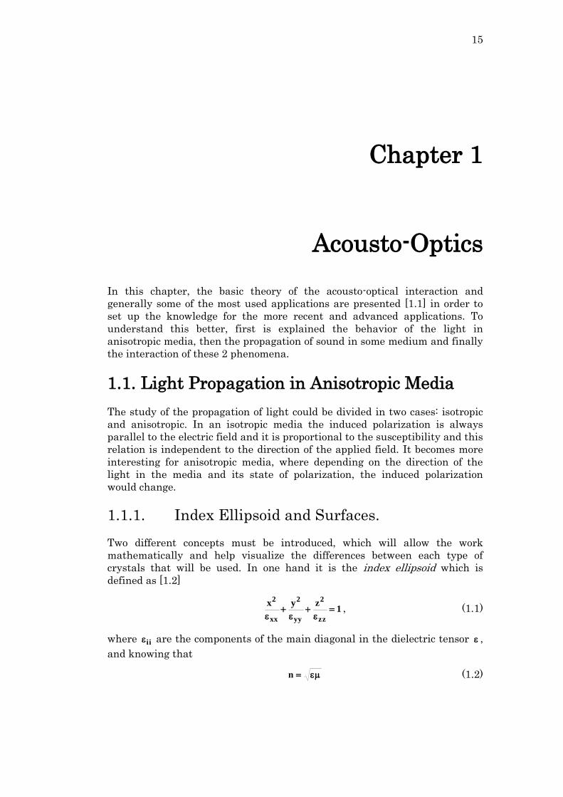
ellipse, see Fig. 1.1, which will have the following properties:
Figure 1.1 The index ellipsoid for a uniaxial medium. The shaded ellipse is
perpendicular to the k
vector
1) The axes of this ellipse define two orthogonal directions for the electric
displacement D
which satisfy simultaneously the Maxwell’s equations
and the constitutive relation
ED 0
. (1.5)
one of the two axes is always in the yx plane and correspond to the
direction of polarization of the ordinary wave and its length is
independent of the direction of k
. The other axes is related to the
extraordinary wave and its length depends on the angle between k
and the z axis.
17
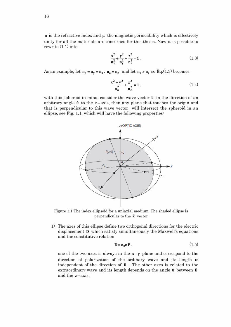
2) The length of the semi-axis of the ellipse are the refractive indices,
on for the ordinary wave and )(n~e for the extraordinary wave. The
value of )(n~e is easily estimated from Fig. 1.2. The length of the bold
line perpendicular to k in Fig. 1.2 is the value of
2e
2
2o
2
en
sin
n
cos)(n~
. (1.6)
On the other hand there are the index surfaces which represent the values of
the refractive indices for all the possible directions of propagation of the wave
vector k
.
Using the previous example, the index surface would look like Fig. 1.3b or
1.3c. The planes of polarization for the ordinary and extraordinary are
perpendicular, this characteristic will be particularly useful for some
applications listed in subsection 1.5.
The present work is focused on this representation and it will be explained for
the different crystal types in the next section.
Figure 1.2 Projection of the index ellipsoid into the zk plane.
1.1.2. Crystals; Optically Isotropic, Uniaxial and
Biaxial
In crystals, the optical isotropy is observed in cubic crystal systems (also
applicable for amorphous media), in these systems the dielectric tensor is
given by
2
2
2
0
n00
0n0
00n
, (1.7)
18
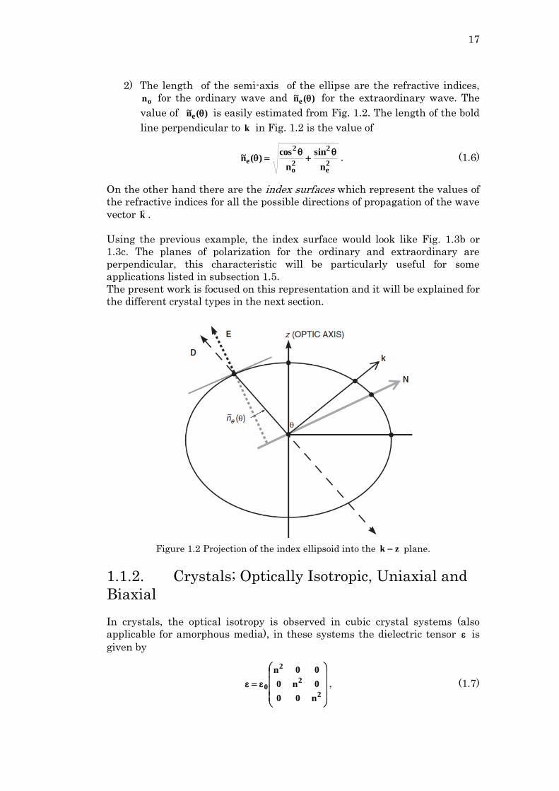
where 0 is the permittivity of vacuum. In Fig. 1.3a is shown the expected
index surface for this case which is the simplest one.
Figure 1.3 Index surfaces for: (a) isotropic, (b) positive uniaxial, (c) negative
uniaxial, and (d) biaxial medium.
There also exist the uniaxial crystals; these ones are crystals systems of
tetragonal, hexagonal and trigonal kind. Their dielectric tensor is of the form:
2e
2o
2o
0
n00
0n0
00n
, (1.8)
being on the ordinary and en the extraordinary refractive index. In Fig. 1.3b
and 1.3c it is seen the two cases for its index surface, if oe nn it is called
‘positive uniaxial’ and if oe nn it is called ‘negative uniaxial’.
The biaxial crystals represent the most complicated case. The index surfaces
for this type of crystal is shown in Fig. 1.3d. Its dielectric tensor is
represented as
2z
2y
2x
0
n00
0n0
00n
. (1.9)
1.2. Ultrasound Propagation in Anisotropic
Media
The acoustic propagation is much more complicated than the light
propagation, in the light wave what oscillates is the electromagnetic field but
in the acoustic waves are the positions of the atoms/molecules.
Strain tensor This tensor is related to the deformation of a body. In some coordinate system
the position of any point is defined by a vector 32i xz,xy,xxr
. When the
body is deformed this position changes to a new vector i'x'r , and this
displacement is given by the vector r'ru
;
iii x'xu , (1.10)
19
which is called the displacement vector. When a body is deformed, the
distance between two points will change. Let us consider two very close points
with the radius vector joining the points as idx , the vector joining this points
when deformed will be iii dudx'dx . Here the squared distance between the
points is 2i
2dxdl before the deformation and 2ii
2i
2dudx'dx'dl after the
deformation. Now kkii dxxudu is substituted to rewrite
lkl
i
k
iki
k
i22dxdx
x
u
x
udxdx
x
u2dl'dl
,
the second term on the right can be rewritten as
.dxdxx
u
x
uki
i
k
k
i
and then, in the third term the suffixes i and l are interchanged so
kiik22
dxdxu2dl'dl , (1.11)
where the tensor iku is defined as
k
l
k
l
i
k
k
iik
x
u
x
u
x
u
x
u
2
1u . (1.12)
iku is called the strain tensor. This tensor represents the change in the
distance between two points when a body is deformed. In this case, the body
is a crystal and the deformation is caused by the acoustic wave. It is easy to
see, from Eq. (1.12), the symmetry of the strain tensor,
kiik uu . (1.13)
Because of this symmetry the strain tensor can be diagonalized at any given
point. When diagonalized at a given point, the element of length, Eq. (1.11),
becomes
23
322
221
12dx)u21(dx)u21(dx)u21('dl ,
where iu is the component of the diagonal of iiu . From this expression is
possible to see that the strain tensor is the sum of three independent
directions mutually perpendicular.
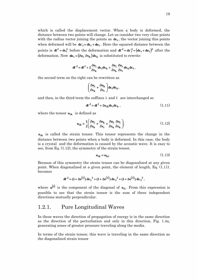
1.2.1. Pure Longitudinal Waves
In these waves the direction of propagation of energy is in the same direction
as the direction of the perturbation and only in this direction, Fig. 1.4a,
generating zones of greater pressure traveling along the media.
In terms of the strain tensor, this wave is traveling in the same direction as
the diagonalized strain tensor
20
1.2.2. Pure Shear Waves
Now the acoustic wave, in contrast with the longitudinal wave, makes the
oscillation of the particles perpendicular to the direction of propagation, see
Fig. 1.4b. Shear waves are slower than longitudinal waves and this will make
them very useful for the acousto-optical applications explained later.
In terms of the strain tensor, this wave is traveling perpendicular to the
direction of iiu .
Figure 1.4 Acoustic waves in a medium; (a) pure longitudinal wave and (b) pure shear
wave.
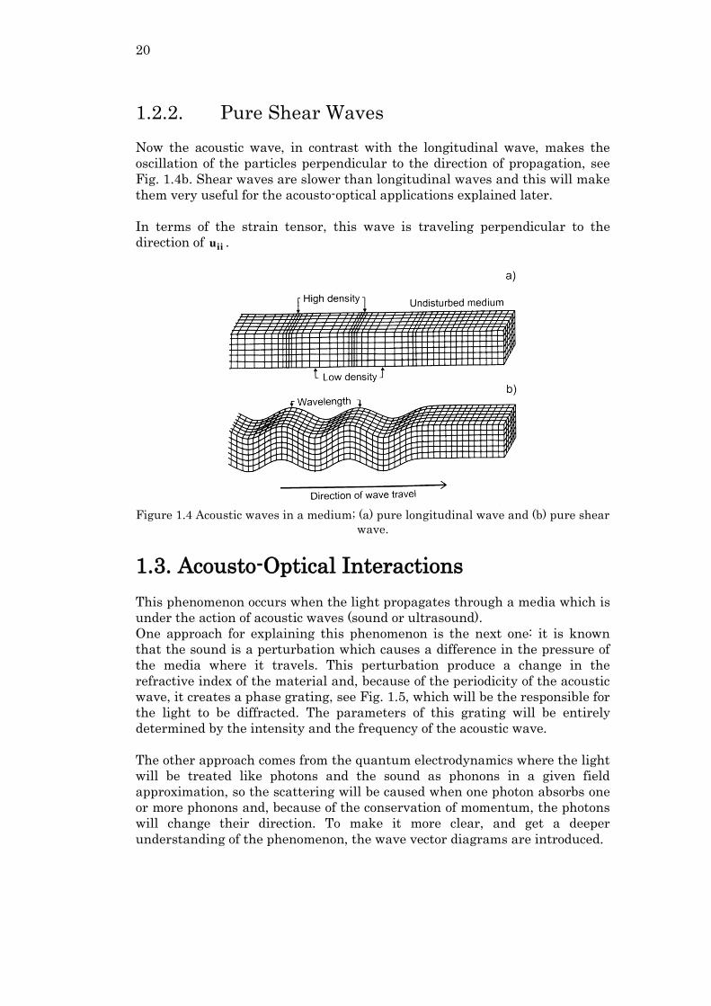
1.3. Acousto-Optical Interactions
This phenomenon occurs when the light propagates through a media which is
under the action of acoustic waves (sound or ultrasound).
One approach for explaining this phenomenon is the next one: it is known
that the sound is a perturbation which causes a difference in the pressure of
the media where it travels. This perturbation produce a change in the
refractive index of the material and, because of the periodicity of the acoustic
wave, it creates a phase grating, see Fig. 1.5, which will be the responsible for
the light to be diffracted. The parameters of this grating will be entirely
determined by the intensity and the frequency of the acoustic wave.
The other approach comes from the quantum electrodynamics where the light
will be treated like photons and the sound as phonons in a given field
approximation, so the scattering will be caused when one photon absorbs one
or more phonons and, because of the conservation of momentum, the photons
will change their direction. To make it more clear, and get a deeper
understanding of the phenomenon, the wave vector diagrams are introduced.
21
Figure 1.5 Acoustic wave traveling in a crystalline material and generating a phase
grating. L is the interaction length, D is the aperture of the cell, is the acoustic
wavelength, and B is the Bragg angle.
1.3.1. Wave Vector Diagrams; Normal and
Anomalous Light Scattering
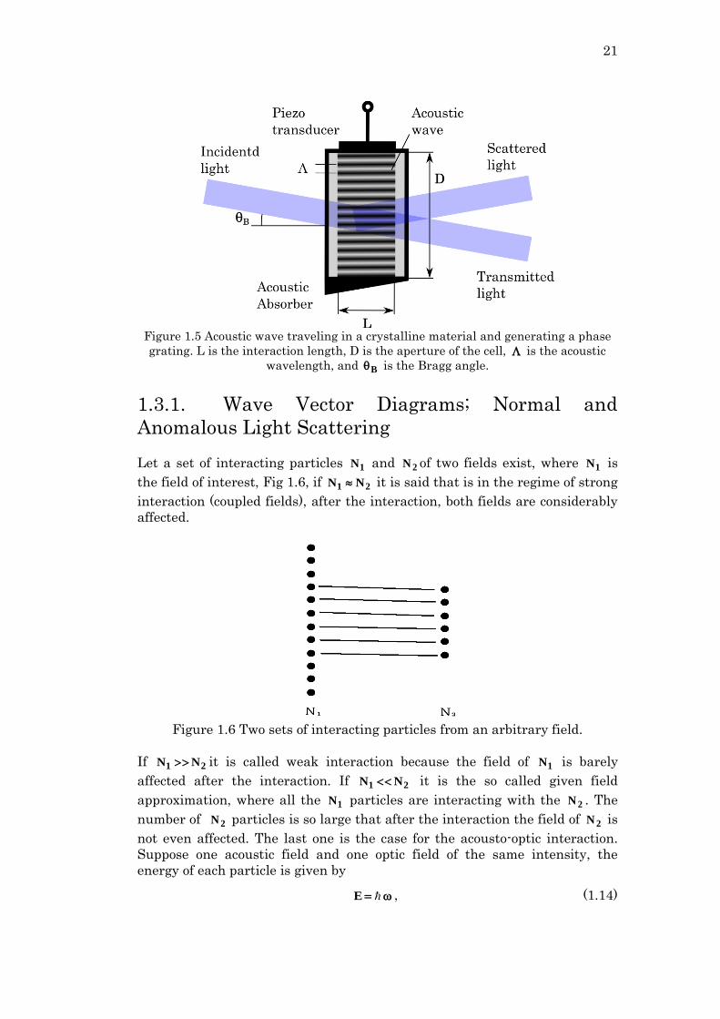
Let a set of interacting particles 1N and 2N of two fields exist, where 1N is
the field of interest, Fig 1.6, if 21 NN it is said that is in the regime of strong
interaction (coupled fields), after the interaction, both fields are considerably
affected.
Figure 1.6 Two sets of interacting particles from an arbitrary field.
If 21 NN it is called weak interaction because the field of 1N is barely
affected after the interaction. If 21 NN it is the so called given field
approximation, where all the 1N particles are interacting with the 2N . The
number of 2N particles is so large that after the interaction the field of 2N is
not even affected. The last one is the case for the acousto-optic interaction.
Suppose one acoustic field and one optic field of the same intensity, the
energy of each particle is given by
E , (1.14)
22
where is the Planck constant divided by 2 and is the frequency of the
particle. For the photons Hz1014
L , and for the phonons Hz109
A , in
order to have more or less the same energy in both fields there would be 5
10 more phonons than photons, AL NN so it is possible to use the given
field approximation for the acoustic field.
In every physical interaction there are some measurable properties that must
be conserved, for this subject, these ones are the energy and the linear
momentum. In quantum mechanics, the linear momentum of a particle is:
kp , (1.15)
where k is the wave vector. So the relations that must be satisfied are:
EEE AL (1.16a)
ppp AL
(1.16b)
where E stands for energy, p for momentum, the subscripts L and A are for
the light and the acoustic fields, and the subscripts is for the scattered
light. Using Eq. (1.14), (1.15), (1.16a) and (1.16b) is possible to arrive to two
conditions:
10 , (1.17a)
10 kKk
, (1.17b)
here the subscripts 0 and 1 are for the incident and the scattered light, from
now on the uppercase greek letter and uppercase K are for the acoustic
frequency and the acoustic wave vector respectively. This conditions can be
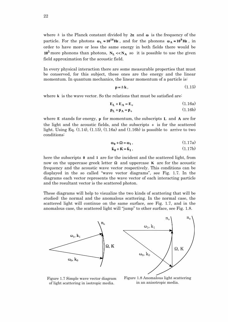
displayed in the so called “wave vector diagrams”, see Fig. 1.7. In the
diagrams each vector represents the wave vector of each interacting particle
and the resultant vector is the scattered photon.
These diagrams will help to visualize the two kinds of scattering that will be
studied: the normal and the anomalous scattering. In the normal case, the
scattered light will continue on the same surface, see Fig. 1.7, and in the
anomalous case, the scattered light will “jump” to other surface, see Fig. 1.8.
Figure 1.8 Anomalous light scattering
in an anisotropic media.
Figure 1.7 Simple wave vector diagram
of light scattering in isotropic media.
23
Note that the anomalous light scattering cannot occur in isotropic media
because there is just one surface. On the other hand, the normal light
scattering can occur on both, isotropic and anisotropic media.
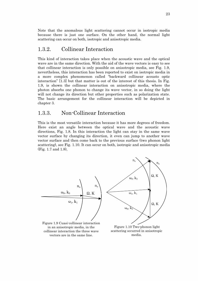
1.3.2. Collinear Interaction
This kind of interaction takes place when the acoustic wave and the optical
wave are in the same direction. With the aid of the wave vectors is easy to see
that collinear interaction is only possible on anisotropic media, see Fig. 1.9,
nevertheless, this interaction has been reported to exist on isotropic media in
a more complex phenomenon called “backward collinear acousto optic
interaction” [1.3] but that matter is out of the interest of this thesis. In Fig.
1.9, is shown the collinear interaction on anisotropic media, where the
photon absorbs one phonon to change its wave vector, in so doing the light
will not change its direction but other properties such as polarization state.
The basic arrangement for the collinear interaction will be depicted in
chapter 3.
1.3.3. Non-Collinear Interaction
This is the most versatile interaction because it has more degrees of freedom.
Here exist an angle between the optical wave and the acoustic wave
directions, Fig. 1.8. In this interaction the light can stay in the same wave
vector surface by changing its direction, it even can jump to another wave
vector surface and then come back to the previous surface (two phonon light
scattering), see Fig. 1.10. It can occur on both, isotropic and anisotropic media
(Fig. 1.7 and 1.8),
Figure 1.9 Cuasi-collinear interaction
in an anisotropic media, in the
collinear interaction the three wave
vectors are in the same line.
Figure 1.10 Two-phonon light
scattering occurred in anisotropic
media.
24
1.4. The Formal Approach (Differential
Equation Method)
This method starts with the Maxwell’s equations for a dielectric medium with
a changing dielectric constant )t,y,x( as a function of position and time. After
some well known operations, the Maxwell’s equations give the differential
equation for the electric field of light as
0Etc
1E
2
2
2
2
(1.18)
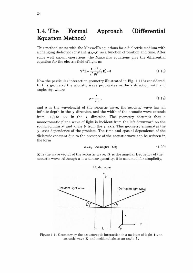
Now the particular interaction geometry illustrated in Fig. 1.11 is considered.
In this geometry the acoustic wave propagates in the x direction with and
angles ±, where
L2
, (1.19)
and is the wavelenght of the acoustic wave, the acoustic wave has an
infinite depth in the y direction, and the width of the acoustic wave extends
from 2L to 2L in the z direction. The geometry assumes that a
monocromatic plane wave of light is incident from the left downward on the
sound column at and angle from the z axis. This geometry eliminates the
y axis dependence of the problem. The time and spatial dependence of the
dielectric constant due to the presence of the acoustic wave can be written in
the form
)tKx(sin0 (1.20)
K is the wave vector of the acoustic wave, is the angular frequency of the
acoustic wave. Although is a tensor quantity, it is assumed, for simplicity,
Figure 1.11 Geometry oy the acousto-optic interaction in a medium of leght L , an
acoustic wave K and incident light at an angle .
25
that it can be represented by a scalar. With this geometry the electric field
can be written in the form
)]tcoskzsinkx(i[expUE 0 (1.21)
Now, it is possible to assume that the solution of the diffracted light is given
by the sum
l
l ]}coskzx)lsink(t)l[(i{exp)z(UE (1.22)
This sum represents a series in plane waves whose amplitudes )z(Ul vary
within the crystal along the z coordinate. Each plane wave, except 0U ,
originates from the absorption or emission of one or more phonons by the
incident light beam in the interaction volume but this particular
representation is only valid for 2,1l .
This solution is substituted into Eq.(1.18). If the amplitude of each of the
diffracted plane waves increases slowly with distance z z, the resulting terms
in 2l
2dzUd can be neglected. Also one can neglect the terms which are
relatively small by the factor 1 and the factor 1cV . Using the
substitutions ck and V , the resulting equations for the amplitude
factors )z(Ul are
0)]z(U)z(U[)z(Ui)z('U 1l1llll (1.23)
where
k2
lsin
cos
ll ,
cos
k
4
1
0l (1.24)
The general solution for the equations system in Eq.(1.23) is very complicated
so it is considered that l1l UU and that initially only 0U0 . The equation
for lU can be written as
1lll UUi
z
U
(1.25)
The solution for this differential equation can be written in the form
z
l1lll 'dz)'zi(expU)zi(expU (1.26)
Now the case 1l is considered, it corresponds to the first order diffraction. If
the acoustic-wave amplitude is uniform and nonzero only in the range 2L to
2L , then is constant and nonzero only within the same limits. And, since
01 UU , it is assumed that the diffraction process removes a negligible
fraction of the incident light beam power. Thus, 0U is basically constant in
value and the amplitude of the first order diffracted light is
2/L
2/L101l 'dz)'zi(expU)zi(expU
26
2/L
)2/L(sinLU)zi(expU
1
101l
(1.27)
where
k2sin
cos1 (1.28)
Using Eq.(1.23) is possible to estimate the fractional amount of light intensity
which is diffracted by the acoustic wave as
21
12
221
00
11
0
1
)2/L(
)2/L(sinL
*UU
*UU
I
I
(1.29)
The maximum amount of power diffracted into one order occurs when 01 .
For this condition,
21
0
1 )L(I
(max)I (1.30)
Second order diffraction occurs when the light beam is scattered by two
phonons. Using Eq. (1.21) and solving the equation system while assuming
that l1l UU and 0U0 , is possible to find the amplitude for the second
order diffraction. This gives
02
2212
12
22
UUdz
dUi2
dz
Ud (1.31)
Neglecting the first term and assuming that the amplitude of the acoustic
wave is uniform and nonzero between 2L to 2L gives the result
4/L
)4/L(sin
2
ziexp
i2
LUU
2
22
1
02
2
(1.32)
The use of Bragg diffraction is based on the results obtained in Eqs.(1.26)
which express the diffracted light amplitude in terms of the scattering
parameters and the experimental conditions. Using the particular case of an
optical beam passing through a uniform-intensity acoustic beam of width L ,
the diffracted light amplitude for the second order is Eq. (1.32). where, using
Eq. (1.24)
cos
ksin2
2
cos
k
4
1
02
The central maximum of the diffraction pattern occurs when 02 , which
leads to
sink
(1.33)
27
where V
f
k
c
, V is the speed of the acoustic wave, cf is the central
frequency of the scattered light and is the wavelength inside the material.
The relative peak intensity of the diffracted beam is
1
02
22
LUU
. (1.34)
By differentiating Eq. (1.33), one obtains the diffraction bandwidth
L
cosV2
f
(1.35)
1.5. Applications of Modulation, Filtering and
Deflection
There are several applications for acousto-optics and each one can reach
different limits according to the materials and techniques used. Here is
presented a brief explanation of the three applications which will be exploited
in this thesis.
Light Modulation This application consist in the modulation of light intensity of one selected
diffraction order, usually the first order, while blocking the rest of the orders.
The modulation of the selected order is achieved by increasing the diffraction
efficiency given by
21
peak
a2
in
1
P
P
2sin
I
I
, (1.36)
defined as the ratio of the power of the first order divided by the incident light
power, aP is the acoustic beam power and peakP is the power of the peak
diffraction efficiency.
For the zeroth-order, the diffraction efficiency can be approximated by the
complement of the first-order diffraction efficiency;
21
peak
a2
in
0
P
P
2cos
I
I
. (1.37)
The major performance is given by the response time related to the transit
time defined as the time required for the acoustic beam to travels through
the light beam,
s
in
V
D , (1.38)
where inD is the diameter of the light beam and sV is the velocity of the sound
in the media.
28
Deflection It is used for very precise deflection of light beams, the acousto-optic (AO)
deflector designed to diffracts a collimated light beam into a single order
whose spatial position will be determined by the frequency of the acoustic
wave applied to the device. When working in the Bragg regime, it is called
Bragg cell. Using the conservation of momentum is possible to estimate the
angle of deflection,
Kkk id
(1.39)
where dk
is the wave vector of the deflected light, ik
for the incident light
and K
for the acoustic wave, which magnitude is:
Bsink2K , (1.40a)
n2sin 01
B , (1.40b)
here n is the index of refraction of the AO medium, 0 is the free-space
wavelength of the light, and is the acoustic wavelength. B is called the
Bragg angle, note that this is the same angle that maximizes the amount of
light diffracted in Eq. (1.29). When the AO cell is illuminated at this angle,
the total angle of deflection is
nV
f2 0
BD
(1.41)
where f is the frequency of the acoustic wave, so the angle of deflection is
proportional to this frequency.
Filtering Generally, there exist two kinds of AO filters: isotropic AO filters, which use a
pinhole for selectivity, and collinear filters made with anisotropic crystals.
The second kind is more common and this work will focus on that type of
filters. The condition for such an interaction to exist is
Vnf , (1.42)
where oe nnn and is the wavelength of the light in the crystal. The
resolution can be estimated as
L
V1f
, (1.43)
where is the sound transit time and L the collinear interaction length.
Based on this, longer interaction lengths help to improve the frequency
resolution
For optically anisotropic media, the acousto-optical interaction can change
the polarization state of the light, see Fig. 1.8 and 1.9. This can be exploited
to filter the scattered from the non-scattered light using an acousto-optical
cell between crossed polarizers and will be explained in more details in
chapter 3.
29
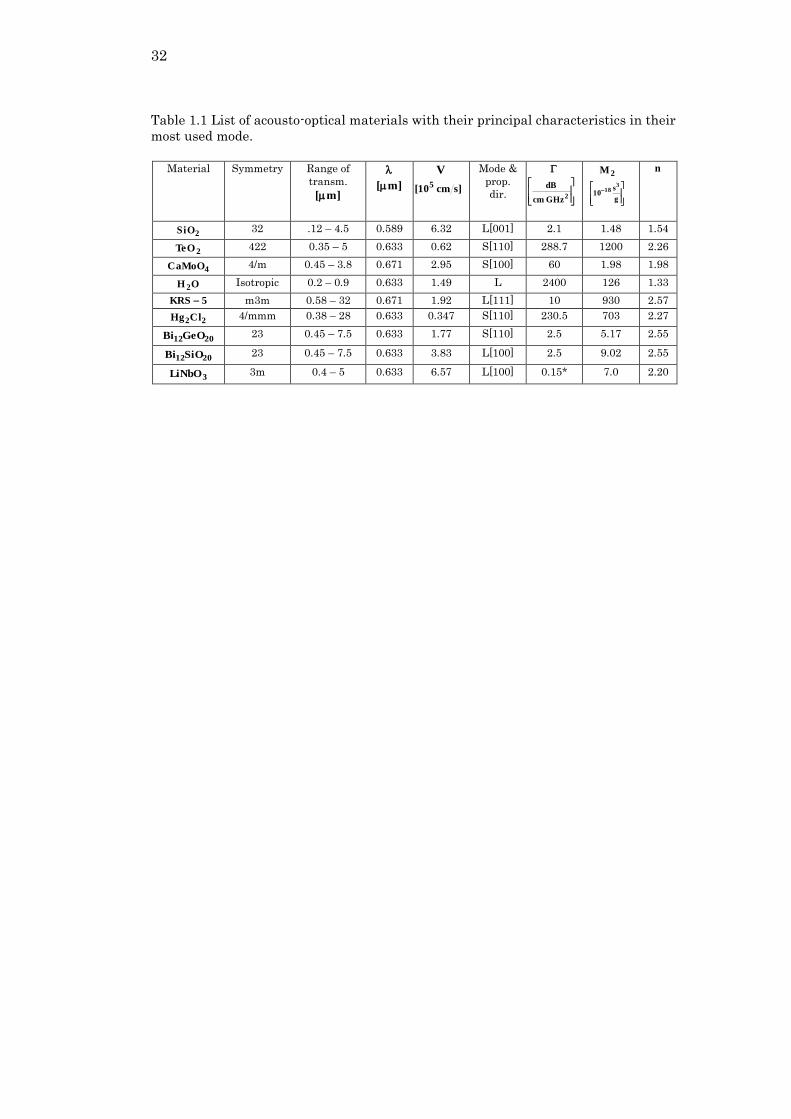
1.6. Acousto-Optic properties of Materials
The most important characteristics concerned for the acousto-optical
interaction are listed and their values for some selected materials are shown
in Table 1.1. When choosing a material to work with, there are several
aspects one look forward, and depending on the selected application, the
material could develop great in some aspect but very bad in other ones. There
is no perfect material and it is necessary to find a balance in its properties to
have the best overall performance, for example; 2TeO has a very large figure
of merit 2M , which is a good quality, but its high acoustic losses set a limit
for its use in some applications.
Range of transmission One of the most important thing to take into account is the range of
transmission. This parameter tell us which light wavelengths are not (or less)
absorbed by the material. Some crystal could have the best acoustic
properties for some specific problem but will be useless if all the light is
absorbed or even reflected.
Sound velocity This parameter can be estimated using considering a simple model of an
array of points of mass M separated a distance a and bounded by springs of
constant C . By taking into account just the nearest neighbor interactions the
sound velocity is [1.4]
M
aCV
2
(1.44)
Measured in scm , this characteristic is closely related with the figure of
merit, which is described later, but also have an important role for generating
the index gratings. As it is known,
V, (1.45)
where V is the velocity of the sound, is the frequency injected by the
piezoelectric transducer, and is the wavelength of the sound, which will be
directly related to the period of the grating. With this in mind, with a small
velocity will be easier to generate gratings with more lines per centimeter
because not too high frequencies on the piezoelectric will be needed.
Acoustic losses
For the study of this characteristic an important parameter is the ratio of the
acoustic wavelength and the mean free path of phonons. The mean free
path, in turn, is the inverse of , the collision time between phonons. If
1 the acoustic losses will come from the lattice phonons in thermal
equilibrium. The other regime, when 1 , is more interesting for this
work. Here the mean free path of thermal phonons is smaller than the
acoustic wavelength. The higher density regions will have greater
temperature than the lower density regions and this will produce thermal
30
conduction between them, as a result, energy from the acoustic wave will be
subtracted. The previous analysis is not enough to explain the experimentally
observed acoustic losses so another mechanism should exist. The Akhiezer
mechanism of sound absorption was formulated to treat this phenomenon
described as a phonon viscosity effect.
The attenuation per unit path length is [1.5]:
VA r
2 , (1.46)
where A is a constant to be determined, r is the relaxation time of the
thermal phonons. With this result one can say that the losses are
proportional to the acoustic frequency and that low-velocity materials have
higher losses than the high-velocity materials.
Figures of Merit The efficiency of the light diffracted at the Bragg angle is [1.6]:
2
0
eff3
3
a2
0
1
cos
Lpn
V
LHP
2I
I
(1.47)
where LHIPa is the acoustic power in a beam of intensity I with width L
and height H . Smith and Korpel in 1965 [1.6] propose 2M as a figure of merit
for materials operating under the Bragg conditions:
3
2eff
6
2V
pnM
, (1.48)
where n is the refractive index, is the density of the material, effp is the
effective photo-elastic constant, and V is the acoustic velocity.
The efficiency is proportional to the acoustic beam width but the bandwidth,
according to Eq. (1.35), is inversely proportional to the beam width. In 1966,
Gordon [1.7] proposed a quantity independent of the width,
H
P
cos
2
V
pnff2 a
30
22eff
7
0
. (1.49)
The factor
V
pnM
2eff
7
1 (1.50)
is another figure of merit for materials used in modulators and deflectors.
In Eq.(1.47) and Eq.(1.49) it was assumed that the acoustic beam height is
larger than the light beam diameter. Reducing the acoustic beam height to
the size of the light beam and using the relation L to have tho same
spreading angles in both optical and acoustic beams, one can get the quantity
[1.8]
31
a30
2
2
2eff
7
0 PcosV
pnf
(1.51)
which is, in contrast with Eq.(1.47) and Eq.(1.49), independent of the sizes of
the acoustic and optical beams. With this, it is possible to set
2
2eff
7
3V
pnM , (1.52)
as the third figure of merit. Each figure of merit will have certain relevance
depending on the conditions of the acoustic-optical cell. For the interest of
this work, the most relevant will be the figure of merit 2M .
Elasto-optic Tensor Also knowing as strain-optic tensor, is a physical quantity which relates the
strain tensor and the index of refraction through the acousto-optical
interaction. This interaction occurs in all states of matter and is described by
klijkl
ij2ij up
n
1
(1.53)
where ij is the change in the optical impermeability tensor, iju is the
strain tensor, and ijklp is the elasto-optic tensor. An acoustic wave in a
crystal change the index ellipsoid of the crystal Eq. (1.1) to
1xx)up( jiklijklij . (1.54)
Due to the symmetry of the strain and the impermeability tensor, the indices
i and j as well as k and l can be permuted. The elasto-optic tensor has the
same symmetry of the quadratic electro-optic tensor [Yariv] so one can use
the contracted indices to simplify Eq. (1.53) to
jij
ij2
upn
1
. (1.55)
Photo-elastic constant This constant can be estimated using the photo-elastic tensor ijklp , the strain
tensor klu , the direction of the sound wave in the crystal 1d
, and the
direction of the interacting light 0d
. The effective photo-elastic constant is
0klijkl1eff dupdp
, 6...,,2,1j,i , (1.56)
and using the Eqs. (1.53) and (1.54) one can rewrite Eq. (1.56) with the
contracted indices to simplify the notation. Equation (1.56) then becomes
0jij1eff dupdp
(1.57)
32
Table 1.1 List of acousto-optical materials with their principal characteristics in their
most used mode.
Material Symmetry
Range of
transm.
]m[
]m[
V
]scm10[5
Mode &
prop.
dir.
2GHzcm
dB
2M
g
s10
318
n
2SiO 32 .12 – 4.5 0.589 6.32 L[001] 2.1 1.48 1.54
2TeO 422 0.35 – 5 0.633 0.62 S[110] 288.7 1200 2.26
4CaMoO 4/m 0.45 – 3.8 0.671 2.95 S[100] 60 1.98 1.98
OH 2 Isotropic 0.2 – 0.9 0.633 1.49 L 2400 126 1.33
5KRS m3m 0.58 – 32 0.671 1.92 L[111] 10 930 2.57
22ClHg 4/mmm 0.38 – 28 0.633 0.347 S[110] 230.5 703 2.27
2012GeOBi 23 0.45 – 7.5 0.633 1.77 S[110] 2.5 5.17 2.55
2012SiOBi 23 0.45 – 7.5 0.633 3.83 L[100] 2.5 9.02 2.55
3LiNbO 3m 0.4 – 5 0.633 6.57 L[100] 0.15* 7.0 2.20
33
1.7. Formulation of Problems
A new acousto-optical dynamic diffraction grating for the spectrometer The Guillermo Haro astrophysical observatory uses an optical spectrometer
with several exchangeable traditional (made of a suitable optical glass i.e.
static in behavior) diffraction gratings as the dispersive elements. Due to the
current needs of astrophysical observations the resolution of spectrometer has
to be changed time to time that can be done only by mechanical substitution
of one static diffraction grating with another one. Every time the static
grating is substituted, the spectrometer needs to be realigned and
recalibrated; however, it leads to potential errors in measurements and losing
very important physically and rather expensive time for the observations. In
order to improve this situation, an alternative for the static diffraction
gratings has been proposed: to use specially designed acousto-optical cell as
the dynamic (i.e. completely electronically tunable) diffraction grating, whose
capabilities will make it possible in the nearest future to replace all the static
diffraction gratings from the spectrometer. The principal advantages of
similar dynamic acousto-optical grating are excluding any mechanical
operations within the observation process, avoiding recalibrations (i.e.
bringing in additional errors) and any losses of time. In connection with this,
the first steps in design of a desirable acousto-optical cell, adequate to the
above-mentioned needs, are considered as the first problem within this thesis.
Acousto-optical filter Usually, the performances of acousto-optical filters, exploited in linear regime
and operated by low-level external electronic signals, are completely
determined by the properties and size of a crystalline material chosen for the
device. Nevertheless, preliminary and more detailed consideration of the
filtering process makes it possible to predict that a specific mechanism of the
acousto-optic nonlinearity capable to regulate performances of the collinear
acousto-optical filter exist and could be used practically. That is why the
possibility of analyze this mechanism theoretically and try to confirm it
experimentally with an advanced filter based on calcium molybdate
( 4CaMoO ) single-crystal and governed by external signals of finite amplitude
is formulated as the second problem within this thesis.
Triple Product Processor Detailed studies in the extra-galactic astronomy and searching the extra-
solar planets are now actual avenues of astrophysical investigations. One of
the most powerful instruments in both these areas is the precise multi-
channel spectrum analysis of radio-wave signals. Recently performed
estimations show that the algorithm of space-and-time integrating could be
definitely suitable for a wideband spectrum analysis with an ultimate
frequency resolution. This algorithm requires an advanced acousto-optical
processor to produce the folded spectrum of those signals, accumulating
advantages of space and time integrating. In a view of similar requirement,
developing a schematic arrangement for the triple product acousto-optical
processor based on at least 3-inch optical components of a top-level quality is
suggested as the third problem for this thesis.
35
Chapter 2
Acousto-Optical Version of
Optical Spectrometer for
Guillermo Haro Observatory
Optical spectrometer of the Guillermo Haro astrophysical observatory
(Mexico) exploits mechanically removable traditional static diffraction
gratings as dispersive elements. There is a set of the static gratings with the
slit-density 50 – 600 lines/mm and optical apertures 9 cm x 9 cm that provide
the first order spectral resolution from 9.6 to 0.8 A/pixel, respectively, in the
range 400 – 1000 nm. However, the needed mechanical manipulations,
namely, replacing the static diffraction gratings with various resolutions and
following recalibration of spectrometer within studying even the same object
are inconvenient and lead to losing rather expensive observation time.
Exploiting an acousto-optical cell is suggested, i.e. the dynamic diffraction
grating tunable electronically, as dispersive element in that
spectrometer.which can realize tuning both the spectral resolution and the
range of observation electronically and exclude filters.
2.1. Introduction
The Boller & Chivens (B & C) Cassegrain spectrographs available at
Guillermo Haro Observatory (GHO) are classical grating spectrographs.
Presently, B & C spectrograph is available on GHO at the 2.12m telescope
with 9 gratings, allowing a good coverage in both dispersion and wavelength
within the CCD sensitivity ranges. The observer can communicate most of the
commands necessary to control the spectrographs through a display console
in the control room.
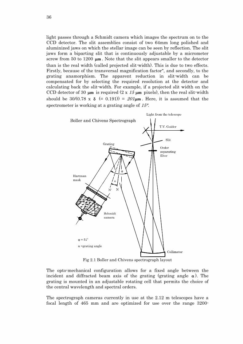
The B & C spectrograph design is shown in Fig. 2.1. The converging light
beam from the telescope passes through the spectrograph entrance slit in the
telescope focal plane to the collimator, an off-axis parabolic mirror. The
reflected parallel beam then falls on to the grating surface. The diffracted
36
light passes through a Schmidt camera which images the spectrum on to the
CCD detector. The slit assemblies consist of two 64mm long polished and
aluminized jaws on which the stellar image can be seen by reflection. The slit
jaws form a biparting slit that is continuously adjustable by a micrometer
screw from 50 to 1200 m . Note that the slit appears smaller to the detector
than is the real width (called projected slit-width). This is due to two effects.
Firstly, because of the transversal magnification factor", and secondly, to the
grating anamorphism. The apparent reduction in slit-width can be
compensated for by selecting the required resolution at the detector and
calculating back the slit-width. For example, if a projected slit width on the
CCD detector of 30 m is required (2 x 15 m pixels), then the real slit-width
should be 30/(0.78 x (= 0.191)) = 201 m . Here, it is assumed that the
spectrometer is working at a grating angle of 15°.
Fig 2.1 Boller and Chivens spectrograph layout
The opto-mechanical configuration allows for a fixed angle between the
incident and diffracted beam axis of the grating (grating angle ). The
grating is mounted in an adjustable rotating cell that permits the choice of
the central wavelength and spectral orders.
The spectrograph cameras currently in use at the 2.12 m telescopes have a
focal length of 465 mm and are optimized for use over the range 3200-
37
12000 Å where they have an efficiency of about 50 - 55 %. Below 3200 Å , the
efficiency drops rapidly to 10% at 3000 Å . A field-flattening lens is also
mounted immediately in front of the CCD dewar in order to correct for
camera field curvature.
An order blocking filter assembly is located below the slit jaws to prevent
overlapping of unwanted spectral orders. The 2.12m spectrograph may hold
up to four filters. The correct choice of filter is normally determined by the
optical group and installed before an observing run. No deckers are used with
the B & C spectrographs for observation. There is a decker mounted in front
of the slit, but this is used for setup purposes only.
Detectors The CCD detector of the Boller & Chivens spectrograph is a back illuminated
Tektronix chip of format 1024x1024 pixels (TK1024AB grade 1)
Calibration Lamps Calibration lamps are mounted at 2.12m, one blue halogen lamp for flat-
fielding and one Helium-Argon spectral lamp for wavelength calibration.
Lamp selection and illumination is done remotely. A neutral density wheel is
also available at the 2.12m. These can be used to attenuate both the He-Ar
and the internal flat-field lamps.
Instrumental Rotation The Cassegrain adapters on telescope can be rotated up to 180º in either
direction. For the 2.12m telescope, the rotation has to be done manually in
the dome. This Cassegrain adapters have scales for accurately setting the
position angles of the spectrograph slit. Instrument rotation can be done with
the 3.6m telescope at any zenith distance. However, since the rotation at the
2.12m telescope is done manually, this is usually done with the telescope at
the zenith to facilitate reading of the position angle scale on the Cassegrain
adaptor. This is particularly important for the 2.12m telescopes, since, once
the spectrograph is unclamped ready for rotation, it may start to rotate
rapidly as the spectrograph is not balanced about the optical axis.
TV Acquisition and Guiding The front surfaces of the spectrograph slits are aluminized and tilted slightly
with respect to the incoming beam to allow the use of an integrating TV
acquisition and guiding system. There is also a "field-viewing" position
(approximate field, 5' x 4') for object acquisition. A visual magnitude (V) ~ 20
mag star can be seen without integration on a moonless night on the center
field camera. The 2.12m telescope also has an intensified camera for auto
guiding. Under good moonless conditions stars of V ~ 18 can be seen. Note
that these are approximate magnitudes and critically depend on focusing,
seeing etc.
38
2.2. Guillermo Haro Observatory Spectrograph
Performances
Available Gratings The Observatory has 9 gratings available. All gratings are 90 x 90 mm and
are used mostly in the first and second order with dispersions ranging from
29 to 450 -1mmÅ .
For some gratings, the astronomer must consider the different efficiencies
encountered for the polarization directions both parallel and normal to the
grooves, especially for highly polarized objects. For most astronomical
observations, however, the average between the two polarization efficiencies
is sufficiently accurate.
Spectral Coverage The grating dispersion, camera focal length, and detector size determine the
observable spectral range. For example, grating # 21, which has a dispersion
of 172 Å1
mm , when used in the first order will provide a spectral coverage
of 172 X 15.36 = 2642 Å with a high resolution RCA chip (1024 X 15 m =
15.36 mm). Given that the grating is centered at 5400 Å , the wavelength
limits will be 4079 Å and 6721 Å .
Spectral Resolution The theoretical spectral resolution depends on the grating dispersion, grating
position, pixel size, collimator and camera focal length, and entrance slit-
width. The effective CCD spectral resolution also depends on the detector
sampling. A detailed calculation of these parameters is shown later in this
text.
As an example, a grating with blaze angle 6°54', centered for Å5400 will have
theoretical resolutions of 1.72 and 3.45 Å for slit-widths of 1" and 2"
respectively. Decreasing the entrance slit-width will improve the resolution.
However, this will be possible only when the sampling requirements (Nyquist
criterion; one resolution element imaged onto at least two detector elements)
are respected and also when the instrumental response is not diffraction
limited.
Spatial Resolution The spatial resolution depends on the transversal magnification factor of the
spectrograph given in Table 2.1. (This spatial scale can easily be determined
by moving a star a known distance along the slit and taking an exposure at
both positions.
The CCD control program allows the CCD pixels to be binned in either
direction (spatial or dispersion) before reading out. This can be an advantage
when the objects are faint in which case may be wanted to bin in the spatial
direction. No spectral resolution will be lost but there will be a decrease in
the read-out-noise by a factor of the square root of the number of pixels
binned. Therefore, this may allow the use of shorter exposure times and
higher signal-to-noise ratios at the cost of decreased spatial and/or spectral
39
resolutions, depending on which direction you are binning. Also, binning
increases the risk of cosmic ray events influencing data since several pixels
are averaged before readout. Furthermore, binning also reduces the contrast
of particle events making automatic removal more difficult. Should spectral
resolution be of vital importance, bin the chip only along the X (spatial)
direction.
The CCD program also allows "readout windowing". This means that only
those pixels within a predefined window or area on the chip are recorded. The
spectrograph slits do not extend across the entire width of the CCDs and
therefore no information is contained outside the length of the slit.
Windowing can thus provide significant savings in the sizes of your data files
and image display time.
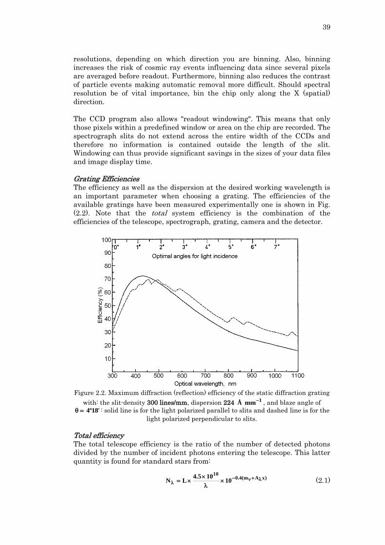
Grating Efficiencies The efficiency as well as the dispersion at the desired working wavelength is
an important parameter when choosing a grating. The efficiencies of the
available gratings have been measured experimentally one is shown in Fig.
(2.2). Note that the total system efficiency is the combination of the
efficiencies of the telescope, spectrograph, grating, camera and the detector.
Figure 2.2. Maximum diffraction (reflection) efficiency of the static diffraction grating
with: the slit-density 300 lines/mm, dispersion 224 Å 1mm
, and blaze angle of
'18º4 : solid line is for the light polarized parallel to slits and dashed line is for the
light polarized perpendicular to slits.
Total efficiency The total telescope efficiency is the ratio of the number of detected photons
divided by the number of incident photons entering the telescope. This latter
quantity is found for standard stars from:
)xAm(4.010
10105.4
LN
(2.1)
40
where, L is the telescope primary mirror area in square meters and N . is the
number of photons at wavelength incident on the telescope per second and
Angstrom. A . is the mean extinction coefficient and x is the airmass. The
values of m are found from tables of standard stars.
Expected S/N ratios The expected S/N ratio obtained by a CCD with a finite read-out-noise and
dark current, is:
5.022r
1)0mm(4.00
)0mm(4.00
]tD)Nb(10tn3600[
10tn3600
N
S
(2.2)
where 0n is the efficiency in e-1s-1pixel-1 for a star of magnitude 0m , is the
width of the spectrum in pixels, perpendicular to dispersion, rN is the read-
out-noise in 11pixele
, D is dark current in 111hrpixele
, t is the exposure
time in hours, b is the binning factor perpendicular to the dispersion
direction, and m is the stellar magnitude.
2.2.1. Calculations for the Spectral Resolutions
Here, it is presented the formulae for deriving the spectral resolution.
)2cos(102
nmsin
7
1 (2.3)
)2cos(
)2cos(
f
f'
1
2 (2.4)
2
7
fmn
)2cos(10D (2.5)
1
4
sfmn
)2cos(10'DR (2.6)
where is the central wavelength in Å , n is the number of lines per mm , m
is the diffraction order, is the grating configuration angle (see Fig. 2.3), is
the grating angle, is the entrance slit-width in m , ' is the projected slit-
width in m , 1f is the collimator focal length in mm , 2f is the camera focal
length in mm , D is the dispersion in -1mmÅ , sR is the theoretical
spectrograph resolution in Å (without detector), and 12 ff is the
transversal magnification factor
The effective CCD.spectral resolution is the convolution of sR with the
detector pixel size. With suitable detector sizes, the spectrum may be
sufficiently sampled to avoid spectral information distortion (eg. line profile
distortions). The common sampling criterion is pixels2Rs (i.e. Nyquist
criterion).
41
2.3. Acousto-Optical Cell
In this chapter the potential use of an acousto-optical cell as a diffraction
grating is discussed. In order to apply this for the design of the spectrograph,
the parameters of the diffraction gratings, currently used, must be know, also
its performance. Later, the analysis of the performance of the acousto-optic
phase grating needs to be made to compare it with the previous gratings.
2.3.1. The nature of Acousto-optical dynamic
diffraction grating
Photo-elastic effect consists in connection between the mechanical
deformations or stresses and the optical refraction index n . This effect
takes place for all the condensed matters and mathematically can be
explained as [2.1]
lklkjilklkji
ji2ji p
n
1
, (2.7)
where ji2
ji )n/1( represents varying the tensor of optical
impermeability or, what is the same, the parameters for an ellipsoid of optical
refractive indices; while p and are the tensors of photo-elastic and piezo-
optical coefficients, respectively. Usually, the higher-order terms relative to
the deformations or the stresses are omitted due to smallness about 510
of both the deformations and/or the stresses . The symmetry inherent in
a medium determines non-zero factors of the tensors p and . With non-zero
external mechanical perturbations, an ellipsoid for the refractive indices can
be explained by
1xxn
1
n
1ji
ji2
ji2
j,i
, (2.8)
Due to all the tensors , p , and are symmetrical in behavior, one can use
so-called matrix indices [2.1]. Now, let us consider propagation of the
traveling harmonic longitudinal elastic wave along the ||z
]001[ -axes through
an isotropic medium, so that the displacement u of particles is described by
)xKt(cosU)t,x(u 333 , where ,,U and K are the amplitude, cyclic
frequency, and wave number of that traveling elastic wave, respectively. The
field of linear deformations ])x/u()x/u([)2/1( ijjiji , occurred by
this wave, is )xKt(sinUK 333 . The components of the optical
impermeability tensor can be written as
a) )xKt(sinUKp 3122211 , b) )xKt(sinUKp 31133 , 2.9)
while 0ji for the indices ji . Here, mnp are the components of the
photo-elastic tensor p with matrix indices. In this case, Eq.(2.8) gives
42
223122
213122
x)xKt(sinUKpn
1x)xKt(sinUKp
n
1
1x)xKt(sinUKpn
1 233112
. (2.10)
Due to Eq.(2.10) does not include any cross-terms, the main axes inherent in
a new ellipsoid for the refractive indices will have the same directions as
before. Consequently, new main values jN of the refractive indices can
explained as
a) )xKt(sinUKpn2
1nNN 312
321 ,
b) )xKt(sinUKpn2
1nN 311
33 . (2.11)
These equations mean that in the presence of the traveling acoustic wave, the
taken isotropic medium becomes a periodic structure, which is equivalent to a
bulk grating with the grating constant equal to the acoustic wavelength
K/2 , because variations in the main refractive indices 33123
2,1 pnn
and 33113
3 pnn are proportional to the amplitudes of displacement or/and
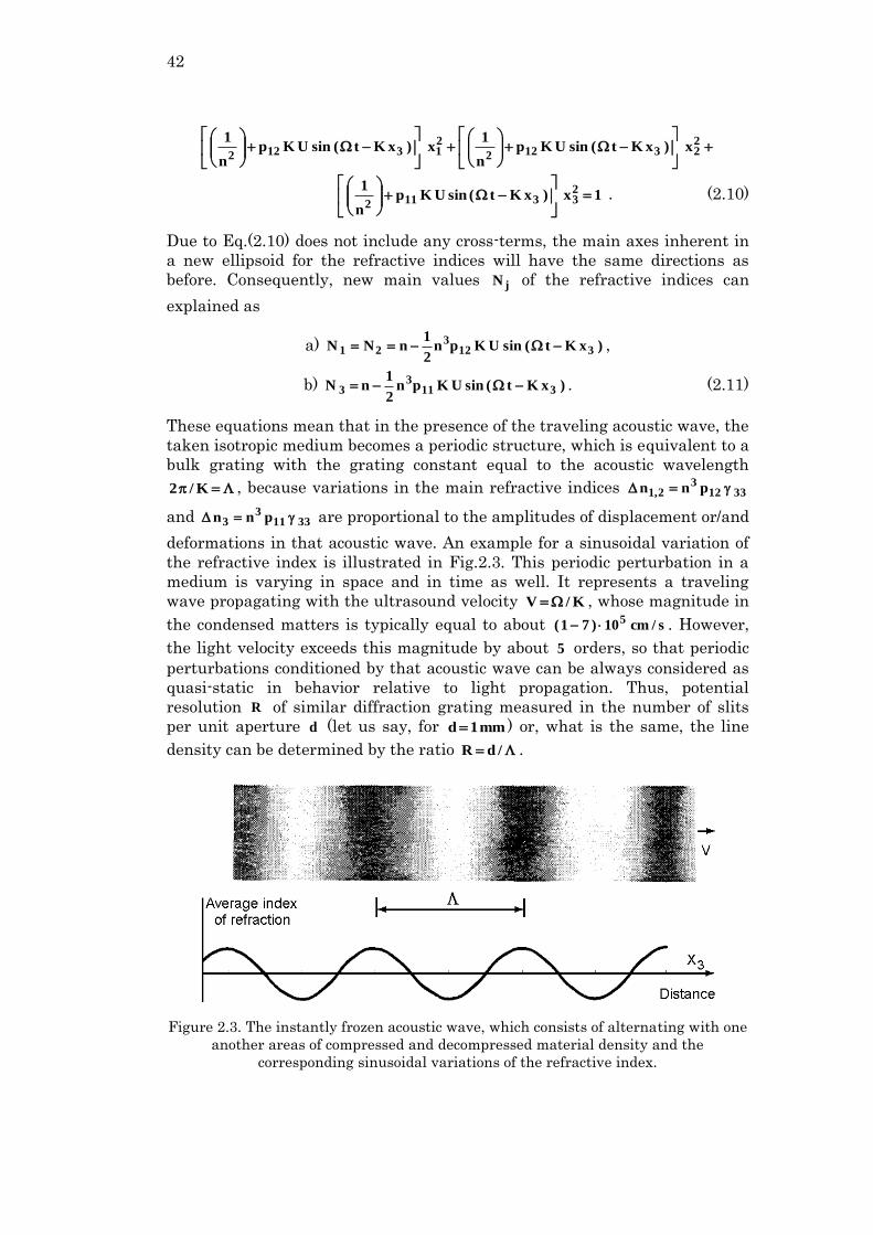
deformations in that acoustic wave. An example for a sinusoidal variation of
the refractive index is illustrated in Fig.2.3. This periodic perturbation in a
medium is varying in space and in time as well. It represents a traveling
wave propagating with the ultrasound velocity K/V , whose magnitude in
the condensed matters is typically equal to about s/cm10)71(5 . However,
the light velocity exceeds this magnitude by about 5 orders, so that periodic
perturbations conditioned by that acoustic wave can be always considered as
quasi-static in behavior relative to light propagation. Thus, potential
resolution R of similar diffraction grating measured in the number of slits
per unit aperture d (let us say, for mm1d ) or, what is the same, the line
density can be determined by the ratio /dR .
Figure 2.3. The instantly frozen acoustic wave, which consists of alternating with one
another areas of compressed and decompressed material density and the
corresponding sinusoidal variations of the refractive index.
43
2.3.2. Requirements and Design
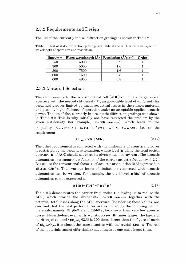
The list of the, currently in use, diffraction gratings is shown in Table 2.1.
Table 2.1 List of static diffraction gratings available at the GHO with their specific
wavelength of operation and resolution.
lines/mm Blaze wavelength (Å) Resolution (Å/pixel) Order 150 5000 3.2 1 300 5000 1.6 1 300 7500 1.6 1 600 7500 0.8 1 600 4850 0.8 1
2.3.3. Material Selection
The requirements to the acousto-optical cell (AOC) combine a large optical
aperture with the needed slit-density R , an acceptable level of uniformity for
acoustical grooves limited by linear acoustical losses in the chosen material,
and possibly high efficiency of operation under an acceptable applied acoustic
power. The list of the, currently in use, static diffraction gratings was shown
in Table 2.2. This is why initially one have restricted the problem by the
given slit-density (for example, mm/lines300R ), which leads to the
inequality R/1f/V )cm1033.0(3 , where 2/f , i.e. to the
requirement
RVff low ]MHz[ . (2.12)
The other requirement is connected with the uniformity of acoustical grooves
is restricted by the acoustic attenuation, whose level B along the total optical
aperture D of AOC should not exceed a given value, let say dB6 . The acoustic
attenuation is a square-law function of the carrier acoustic frequency f [2.2].
Let us use the conventional factor of acoustic attenuation [2.3] expressed in
)GHzcm/(dB2 . Thus various forms of limitations connected with acoustic
attenuation can be written. For example, the total level ]dB[B of acoustic
attenuation can be expressed as
222RVDfD]dB[B . (2.13)
Table 2.2 demonstrates the carrier frequencies f allowing us to realize the
AOC, which provide the slit-density mm/lines300R together with the
potential total losses along the AOC aperture. Considering those values, one
can find that the best performances are exhibited by the following pair of
materials, namely, 2012GeOBi and 3LiNbO , because of their very low acoustic
losses. Nevertheless, even with acoustic losses 40 times larger, the figure of
merit 2M of calomel ( 22ClHg )[2.3] is 100 times larger than the figure of merit
of 2012GeOBi , it is almost the same situation with the crystal 5KRS . The rest
of the materials cannot offer similar advantages so one must forget them.
44
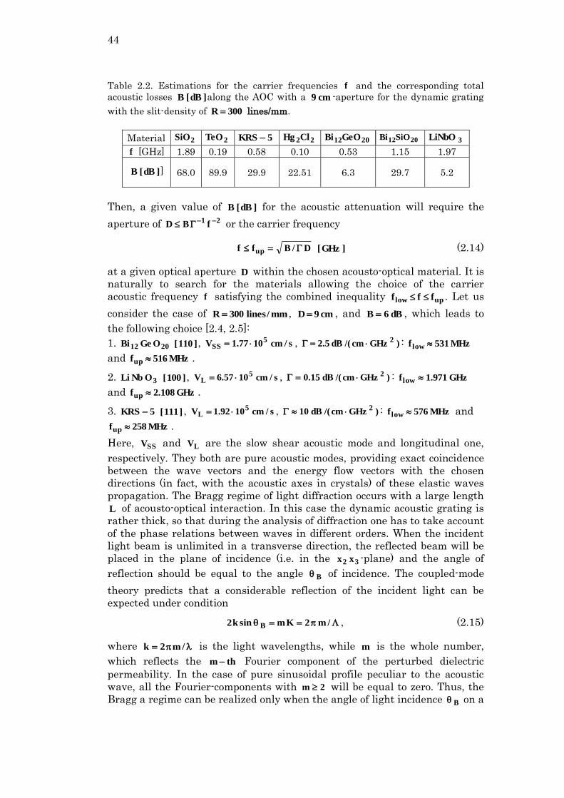
Table 2.2. Estimations for the carrier frequencies f and the corresponding total
acoustic losses ]dB[B along the AOC with a cm9 -aperture for the dynamic grating
with the slit-density of 300R lines/mm.
Material 2SiO 2TeO 5KRS 22ClHg 2012GeOBi 2012SiOBi 3LiNbO
f [GHz] 1.89 0.19 0.58 0.10 0.53 1.15 1.97
]dB[B ] 68.0 89.9 29.9 22.51 6.3 29.7 5.2
Then, a given value of ]dB[B for the acoustic attenuation will require the
aperture of 21fBD or the carrier frequency
D/Bff up ]GHz[ (2.14)
at a given optical aperture D within the chosen acousto-optical material. It is
naturally to search for the materials allowing the choice of the carrier
acoustic frequency f satisfying the combined inequality uplow fff . Let us
consider the case of mm/lines300R , cm9D , and dB6B , which leads to
the following choice [2.4, 2.5]:
1. 2012 OGeBi ]110[ , s/cm1077.1V5
SS , )GHzcm/(dB5.22 : MHz531f low
and MHz516fup .
2. 3ONbLi ]100[ , s/cm1057.6V5
L , )GHzcm/(dB15.02 : GHz971.1flow
and GHz108.2fup .
3. 5KRS ]111[ , s/cm1092.1V5
L , )GHzcm/(dB102 : MHz576f low and
MHz258fup .
Here, SSV and LV are the slow shear acoustic mode and longitudinal one,
respectively. They both are pure acoustic modes, providing exact coincidence
between the wave vectors and the energy flow vectors with the chosen
directions (in fact, with the acoustic axes in crystals) of these elastic waves
propagation. The Bragg regime of light diffraction occurs with a large length
L of acousto-optical interaction. In this case the dynamic acoustic grating is
rather thick, so that during the analysis of diffraction one has to take account
of the phase relations between waves in different orders. When the incident
light beam is unlimited in a transverse direction, the reflected beam will be
placed in the plane of incidence (i.e. in the 32 xx -plane) and the angle of
reflection should be equal to the angle B of incidence. The coupled-mode
theory predicts that a considerable reflection of the incident light can be
expected under condition
/m2Kmsink2 B , (2.15)
where /m2k is the light wavelengths, while m is the whole number,
which reflects the thm Fourier component of the perturbed dielectric
permeability. In the case of pure sinusoidal profile peculiar to the acoustic
wave, all the Fourier-components with 2m will be equal to zero. Thus, the
Bragg a regime can be realized only when the angle of light incidence B on a
45
thick dynamic acoustic grating meets the Bragg condition 2/msin B and
inequality 1/LQ2 for the Klein-Cook parameter [2.6]. Usually, when
an acoustic mode exited by the applied electric signal, the Bragg regime
includes the incident and just one scattered light modes, whose normalized
intensities are described by [2.7]
a) )xq(cosI 12
0 , b) )xq(sinI 12
1 ,
c) 2/PM)cos(q 21
B , d) )V/(pnM
32eff
62 , (2.16)
where 1x is the space coordinate almost along the light propagation; P is the
acoustic power density, is the material density, effp is the effective photo-
elastic constants for light scattering, and n is the averaged effective
refractive index of a material. The Bragg regime is preferable for practical
applications due to an opportunity to realize an %100 efficiency of light
scattering by the acoustic wave. Taking the case of Lx1 in Eq.(2.16b) and
1cos B in Eq.(2.16c), one can find from these equations that the acoustic
power density 0P needed for %100 efficiency of light diffraction into the first
order can be estimated through the requirement 2/Lq in Eq.(2.16b) as
22
2
0ML2
P
. (2.17)
Thus, at the same values of optical wavelength and the interaction length
L , the required acoustic power density will be inversely proportional to the
acousto-optic figure of merit 2M . For the above-mentioned orientations of
crystals, one can cite that 4,5: (1) 2M ( 2012 OGeBi ]110[ , SSV ) g/s1017.5318
and (2) 2M ( 3ONbLi , ]100[ , LV ) g/s100.7318 . For reaching %100 efficiency
of operation at nm500 and cm1L , the following acoustic power densities
0P can be found from Eq.(2.17): (1) 0P ( 2012 OGeBi ]110[ ,
SSV ) 237mm/W242.0s/g1018.24 and (2) 0P ( 3ONbLi , ]100[ ,
LV ) 237mm/W179.0s/g1086.17 .
It should be explained additionally: applying the needed electronic signals at
the electronic input of AOC in such a way that the above-obtained levels of
acoustic power density will be provided makes it possible physically and
potentially technically to achieve %100 efficiency of control over the incident
light diffraction. By the other words, instead of about %70 maximum
efficiency shown in Fig.1 for traditional static diffraction gratings, involving
the acousto-optical technique via creating the dynamic acousto-optical
diffraction gratings is potentially able to provide close to %100 efficiency of
dispersive element over all the range of the above-mentioned spectrum
analysis.
The practical aspects of designing an updated version of the schematic
arrangement for spectrometer under consideration lead first of all to creation
of a modified optical scheme, which has to include some peculiarities of the
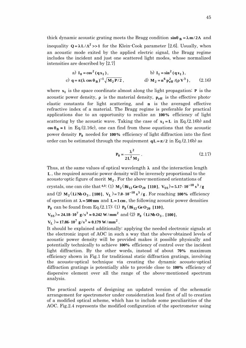
AOC. Fig.2.4 represents the modified configuration of the spectrometer using
46
the AOC as dynamic diffraction grating instead of the static diffraction
gratings; here, B is the Bragg angle of light incidence for the chosen optical
wavelength, see Eq.(2.15). The light coming from the telescope will pass
through the spectrometer entrance slit at the focal plane of the collimator
mirror, the reflected beam, a plane wave, will fall on to the AOC at the Bragg
angle. Then, the diffracted beams corresponding to the first order will be
imaged using a Schmidt-camera and analyzed. An additional modification is
connected with the fact that the acousto-optical dynamic diffraction grating
operates sufficiently effective in the Bragg transit regime instead of the
reflection regime inherent in the above-mentioned classical spectrometer
whose static diffraction gratings exhibit about %70 maximum efficiency.
Figure 2.4. Layout for a new acousto-optical schematic arrangement inserted into the
spectrometer; the proposed dispersive element, i.e. the dynamic diffraction grating is
presented by acousto-optical cell operating in the transit regime of Bragg light
diffraction.
2.4. Diffraction of the light beam of finite width
by a harmonic acoustic wave at low acousto-
optic efficiency
Schematic arrangement of the acousto-optical version of spectrometer, see
Fig. 2.5, exhibits potential presence of optical beams whose widths are
restricted due to condition of observations. This is why the diffraction of light
beam of finite width by harmonic acoustic wave has to be reviewed and
characterized. At first, to illustrate the existing physical tendency simpler let
us start from a low acousto-optical efficiency approximation
47
2221 )x/()x(sin)xq(I , where now 0 is the angular-frequency mismatch.
Due to almost orthogonal geometry of non-collinear acousto-optical
interaction the angles of incidence 0 and diffraction 1 do not exceed
usually about o10 , so that one can use the simplified formulas
a)
n01 ,
b) )(K)K,(2 B00 ,
c)
K)nn(
Kn2
10B , (2.17)
where n is the average refractive index; 1,0n are the refractive indices for the
incident or diffracted light, respectively.
Now, we assume that the area of propagation for a harmonic acoustic wave is
bounded by two planes 0x and Lx in a crystal. This acoustic wave has the
amplitude function ])tzK(i[expu)t,z(u 000 with the amplitude 0u , wave
number 0K , and cyclic frequency 0 , and travels along z -axis. Then, let
initially monochromatic light beam incidents on the area of interaction under
the angle 0 . At the plane 0x , the light field is described by the complex
valued amplitude function )z(ein , reflecting the spatial structure of light
field. The spectra of these fields are [2.8]
a) zd)sinzki(exp)z(e)(E 00in0in
,
b) )KK()ti(expu2)K(U 000 , (2.18)
where 0k is the wave number of the incident light. Each individual
component of the incident light beam is diffracted by the acoustic harmonic in
the interaction area. Using Eqs.(2.17) and (2.18) within taken low acousto-
optical efficiency, the angular spectrum of the diffracted light can be written
as [2.9]
000
1B00in01D d)n2
K(),(T)(E)ti(exp)(E
, (2.19)
2/)(LK
]2/)(LK[sin)Lq(
L
]L[sin)Lq(),(T
B00
B00B0
. (2.20)
Equation (2.19) describes AOC as linear optical system with the transmission
function ),(T B0 , which is real-valued (and positive) within its bandwidth,
i.e. AOC does not insert phase perturbations in the spectrum of optical signal.
When the width inD of the incident light beam is less than acoustic aperture
of AOC, one can say that acoustic beam is infinitely wide, while light beam is
described by the complex amplitude function )D/z(recte)z(e in0in , where
48
1)(rect only when 2/1|| and 0)(rect when 2/1|| . Its angular
Fourier spectrum is given by
/)(Dn
]/)(Dn[sin)De()(E
B0in
B0in00in . (2.21)
Substituting Eq.(2.21) in Eq.(2.19), one can obtain angular distribution for
the diffracted light intensity at low acousto-optical efficiency.
a) 20
20
2in
20
222
1D1D TS)DeLq()(E)(I ,
b)
2
0011
in
0011
in2
20
)n/(Dn
)n/(DnsinS
,
c)
2
0B11
0
0B11
02
20
)n/(L
)n/(LsinT
. (2.22)
The functions 20S and 2
0T represent angular spectra of light and acoustic
beams. The diffracted light structure is determined by overlapping the
functions 20S and 2
0T , i.e. by relation between the light divergence angle
inL Dn/ and the acoustic one L/0S , so that the Gordon parameter
SL /G had been introduced [2.10]. With 1G , the widths of 20S and 2
0T
have the same order. When 1G ( SL ), one can simplify Eq.(2.22a) as
)(I 1D 20
2in
20
22S)DeLq( ; with 1G ( SL ), one yields
20
2in
20
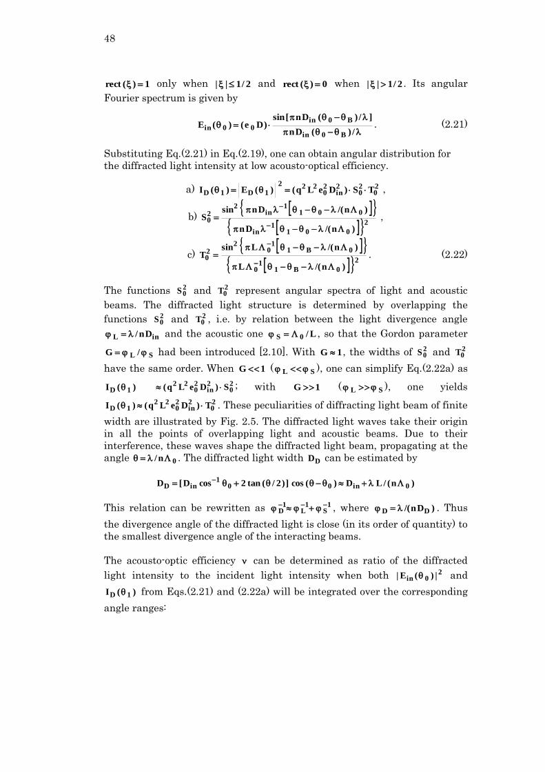
221D T)DeLq()(I . These peculiarities of diffracting light beam of finite
width are illustrated by Fig. 2.5. The diffracted light waves take their origin
in all the points of overlapping light and acoustic beams. Due to their
interference, these waves shape the diffracted light beam, propagating at the
angle 0n/ . The diffracted light width DD can be estimated by
)n(/LD)(cos])2/(tan2cosD[D 0in001
inD
This relation can be rewritten as 1S
1L
1D
, where )Dn/( DD . Thus
the divergence angle of the diffracted light is close (in its order of quantity) to
the smallest divergence angle of the interacting beams.
The acousto-optic efficiency can be determined as ratio of the diffracted
light intensity to the incident light intensity when both 20in |)(E| and
)(I 1D from Eqs.(2.21) and (2.22a) will be integrated over the corresponding
angle ranges:
49
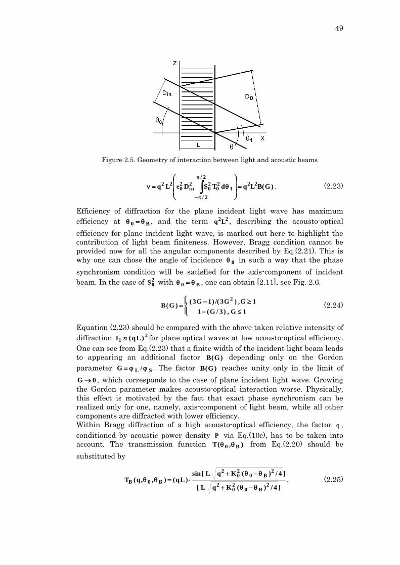
Figure 2.5. Geometry of interaction between light and acoustic beams
)G(BLqdTSDeLq22
2/
2/
120
20
2in
20
22
. (2.23)
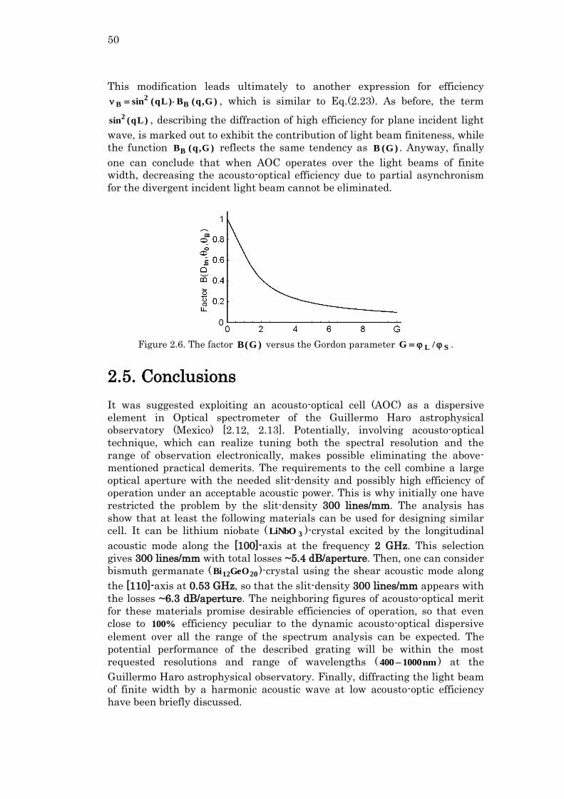
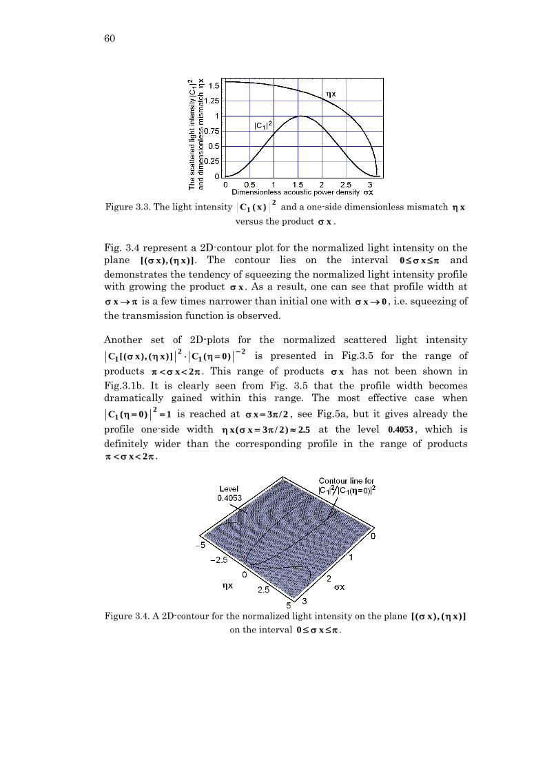
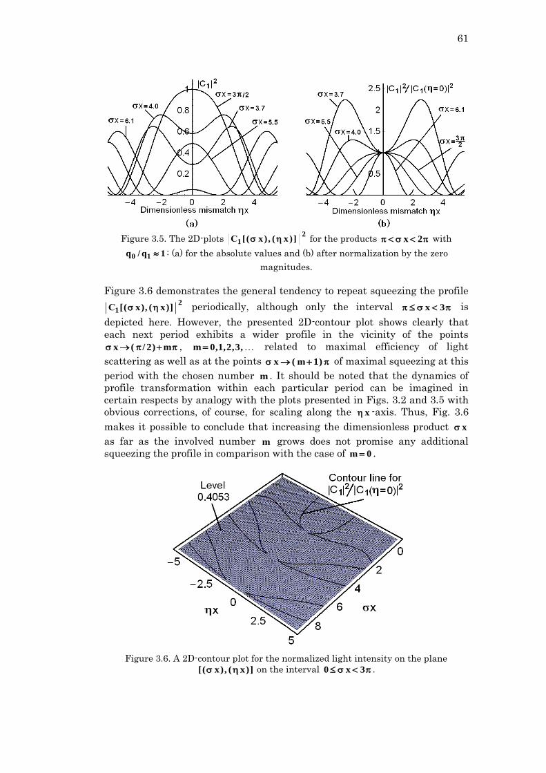
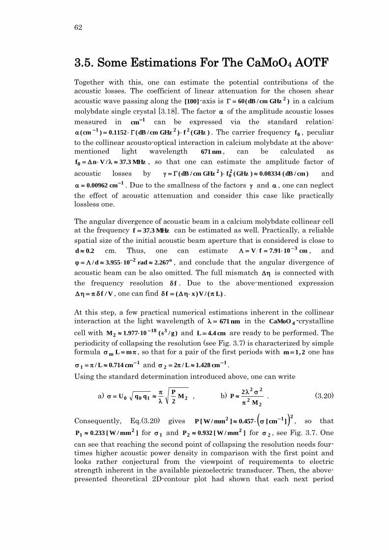
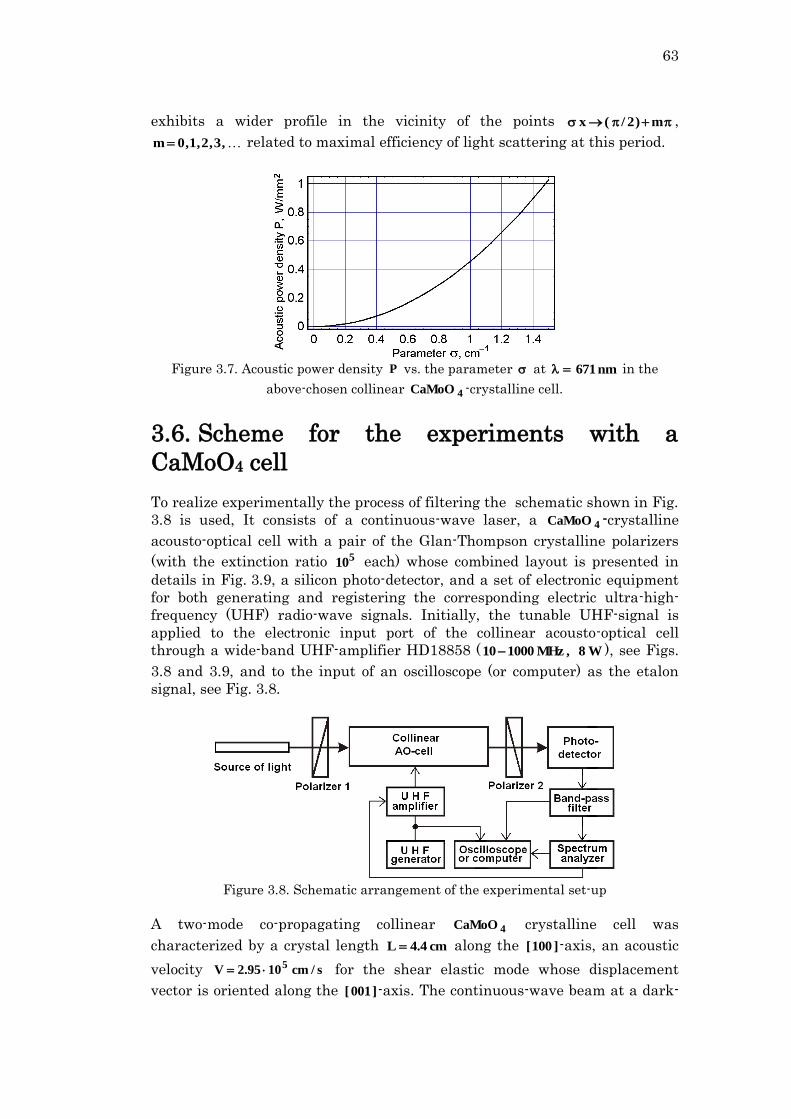
Efficiency of diffraction for the plane incident light wave has maximum
efficiency at B0 , and the term 22Lq , describing the acousto-optical
efficiency for plane incident light wave, is marked out here to highlight the
contribution of light beam finiteness. However, Bragg condition cannot be
provided now for all the angular components described by Eq.(2.21). This is
why one can chose the angle of incidence 0 in such a way that the phase
synchronism condition will be satisfied for the axis-component of incident
beam. In the case of 20S with B0 , one can obtain [2.11], see Fig. 2.6.
1G,)3/G(1
1G,)G3/()1G3()G(B
2
(2.24)
Equation (2.23) should be compared with the above taken relative intensity of
diffraction 21 )Lq(I for plane optical waves at low acousto-optical efficiency.
One can see from Eq.(2.23) that a finite width of the incident light beam leads
to appearing an additional factor )G(B depending only on the Gordon
parameter SL /G . The factor )G(B reaches unity only in the limit of
0G , which corresponds to the case of plane incident light wave. Growing
the Gordon parameter makes acousto-optical interaction worse. Physically,
this effect is motivated by the fact that exact phase synchronism can be
realized only for one, namely, axis-component of light beam, while all other
components are diffracted with lower efficiency.
Within Bragg diffraction of a high acousto-optical efficiency, the factor q ,
conditioned by acoustic power density P via Eq.(10c), has to be taken into
account. The transmission function ),(T B0 from Eq.(2.20) should be
substituted by
]4/)(KqL[
]4/)(KqL[sin)Lq(),,q(T
2B0
20
2
2B0
20
2
B0B
, (2.25)
50
This modification leads ultimately to another expression for efficiency
)G,q(B)Lq(sin B2
B , which is similar to Eq.(2.23). As before, the term
)Lq(sin2 , describing the diffraction of high efficiency for plane incident light
wave, is marked out to exhibit the contribution of light beam finiteness, while
the function )G,q(BB reflects the same tendency as )G(B . Anyway, finally
one can conclude that when AOC operates over the light beams of finite
width, decreasing the acousto-optical efficiency due to partial asynchronism
for the divergent incident light beam cannot be eliminated.
Figure 2.6. The factor )G(B versus the Gordon parameter SL /G .
2.5. Conclusions
It was suggested exploiting an acousto-optical cell (AOC) as a dispersive
element in Optical spectrometer of the Guillermo Haro astrophysical
observatory (Mexico) [2.12, 2.13]. Potentially, involving acousto-optical
technique, which can realize tuning both the spectral resolution and the
range of observation electronically, makes possible eliminating the above-
mentioned practical demerits. The requirements to the cell combine a large
optical aperture with the needed slit-density and possibly high efficiency of
operation under an acceptable acoustic power. This is why initially one have
restricted the problem by the slit-density 300 lines/mm. The analysis has
show that at least the following materials can be used for designing similar
cell. It can be lithium niobate ( 3LiNbO )-crystal excited by the longitudinal
acoustic mode along the [100]-axis at the frequency 2 GHz. This selection
gives 300 lines/mm with total losses ~5.4 dB/aperture. Then, one can consider
bismuth germanate ( 2012GeOBi )-crystal using the shear acoustic mode along
the [110]-axis at 0.53 GHz, so that the slit-density 300 lines/mm appears with
the losses ~6.3 dB/aperture. The neighboring figures of acousto-optical merit
for these materials promise desirable efficiencies of operation, so that even
close to %100 efficiency peculiar to the dynamic acousto-optical dispersive
element over all the range of the spectrum analysis can be expected. The
potential performance of the described grating will be within the most
requested resolutions and range of wavelengths ( nm1000400 ) at the
Guillermo Haro astrophysical observatory. Finally, diffracting the light beam
of finite width by a harmonic acoustic wave at low acousto-optic efficiency
have been briefly discussed.
51
Chapter 3
Transmission Function of
Advanced Collinear Acousto-
Optical Filter
An opportunity for exploiting specific mechanism of the acousto-optic
nonlinearity to regulate performances of the collinear acousto-optical filter,
realizing the sequential spectrum analysis of optical signals, is considered.
This possibility is theoretically analyzed and confirmed experimentally with
an advanced filter based on calcium molybdate ( 4CaMoO ) single-crystal with
a 15 microsecond time-aperture. It is able to operate over red and near-
infrared light at relatively low radio-wave frequencies providing almost
lossless regime for the controlling acoustic waves of the finite amplitude.
Under certain conditions, the transmission function of electronically tunable
filter exhibits a marked dependence on the applied acoustic power density,
and as a result, one can significantly squeeze the transmission function, i.e.
in fact improve the spectral resolution of this filter at the cost of decreasing
the device efficiency partially. The identified and observed non-linear effect
makes possible varying the performance data of similar advanced collinear
acousto-optical filter governed by external signals of the finite amplitude.
3.1. Theory and Operation In 1970 – 80s, novel optical spectral devices, electronically tunable acousto-
optical filters (AOFs) had been proposed and developed. During the years
gone the AOFs have been remarkably progressed, and now they are widely
exploited, for instance, in modern astrophysical observations [3.1, 3.2].
Schematically, the AOFs can be separated on collinear and non-collinear
filters, depending on the relative directions of passing the waves through
crystalline cell within their geometric arrangements, as well as on sequential
and parallel devices, depending on the algorithms realizing for spectrum
analysis of optical signals. Their features are characterized by the amplitude
and spectral parameters. Collinear acousto-optical interaction by itself had
52
been initially predicted and studied in the middle of sixties by R.W. Dixon
[3.3] and then, starting from the seventies has been successfully exploited in
various applications, among which first of all one ought to call the collinear
tunable acousto-optical filters [3.4–8]. The conventional analysis of this
phenomenon in terms of lossless plane waves was presented in a number of
classical issues [3.9, 3.10]. Practically, the methods of acousto-optics had
manifested themselves as rather effective due to their property of quantum
mechanic amplification resulting in the control over high-energetic photons
by low-energetic phonons. The corresponding gain is represented by the direct
ratio of the scattered photon frequency to a frequency of the controlling
phonon frequency. It allows practical application of a given acoustic field
approximation or the regime of a weak coupling, when the spatial
distribution of acoustic beam is almost independent on the spatial
distribution of light that leads to considerable theoretical and practical
facilities. In particular, 100% efficiency of light scattering may be achieved
without any effect on the acoustic beam, so the above-mentioned control can
be repeated for a lot of times with low losses of acoustic energy. Moreover, an
essential difference between velocities of light and ultrasound gives us an
opportunity for applying the quasi-stationary approximation to the analysis
of modern acousto-optical problems. In the past decades great progress has
been made in acousto-optics and now it is a widely used technique in the field
of data processing [3.11]. Nevertheless, recently the existence of a new branch
in studies and applications of collinear acousto-optical interaction, which is
associated with acousto-optical nonlinearity, for example, in the form of
three-wave coupled states, has been manifested [3.12, 3.13]. That is why it is
a worthwhile investment to develop this line more, because the objects being
under consideration here are closely connected with the above-mentioned
nonlinearity in the regime of a weak coupling. Within this consideration, the
exact and closed analytical model of the collinear light scattering by
continuous acoustic waves of the finite amplitude in a birefringent lossless
material is developed. Similar approach definitely includes practically
important case of the presence of really small acoustic attenuation in widely
used acousto-optical filters operating in the traveling-wave regime at
relatively low radio-frequency acoustic waves and exploiting such materials
as quartz or calcium molybdate single crystals. In so doing, the peculiarities
of the effect conditioned by the acousto-optical nonlinearity are analyzed,
which leads to a measurable dependence of the transmission function and
consequently, the spectral resolution peculiar to this filter, on the applied
power density of acoustic waves of finite amplitude in a way allowing, for
instance, to improve the spectral resolution of similar device at the cost of
partial demerit for the filter efficiency.
3.2. Three Wave Collinear Interaction
A three-wave co-directional collinear interaction with the mismatched wave
numbers in a two-mode lossless medium is described by a set of three
nonlinear partial differential equations. Here, the regime of a weak coupling
is considered [3.12, 3.13], when two light modes are scattered by relatively
slow wave, being non-optical by its nature, when essentially effective Bragg
scattering of light can be achieved without any observable influence of the
53
scattering process on that non-optical wave, because the number of
interacting photons is a few orders less than the number of the scattering
quanta injected into a medium. Then, the velocities of light modes can be
approximated by the same value c , because usually the length of crystalline
materials does not exceed cm20 . In this regime, the above-mentioned set of
equations falls into an independent equation for the complex amplitude
)t,x(U of a slow wave ( V is the velocity of this wave) and a pair of the
combined equations for the complex amplitudes )t,x(C0 and )t,x(C1 of the
incident (pumping) light wave and scattered one, respectively,
a) 0t
U
V
1
x
U
, b) xi2expUCq
t
C
c
1
x
C11
00
,
c) xi2expUCqt
C
c
1
x
C00
11
. (3.1)
Here, 1,0q are the constants of interaction and 2 is the mismatch of wave
numbers inherent in the interacting light waves. Now, the tracking
coordinates )cxt,x( are taken into account and assume that non-optical
wave, governed by Eq.(3.1a) and described by )i(exp]V)cV1(x[uU ,
has the constant phase , so that one can convert Eqs.(3.1b) and (3.1c) into
equations of the second order
0Cuqqx
Ci2
x
u
u
1
x
C1,0
210
1,0
2
1,02
. (3.2)
with the condition ])t,x(i[exp)t,x(aC 1,01,01,0 , x1,01,0 and then
divide real and imaginary parts in Eqs.(3.2) as
0a2uqqx
a
x
u
u
1
x
a1,01,0
21,0
210
1,0
2
1,02
, (3.3)
0ax
u
uxx
a2 1,0
1,01,01,01,0
. (3.4)
Equations (3.4) have the following general solutions
21,01,0
21,0
121,01,0 auxd)xa(uau
, (3.5)
where 1,0 are the integration constants. The analysis shows that the
collinear light scattering with 01,0 leads to appearing optical backgrounds.
Within further analysis here, the only regime with 01,0 will be considered
in a view of potential application to filtering optical beams without
backgrounds.
Choosing the simplest case of 01,0 in Eqs.(3.5), one can study the
phenomenon in the continuous-wave regime for both the incident light and
the non-optical wave when 0U]V)cV1(x[u is constant. Equations (3.3)
and (3.4) are analyzed with the fixed magnitude of the mismatch and
54
natural for practice the boundary conditions 1)t,0x(a0 ,
0)t,0x()xa( 0 , 0)t,0x(a1 , 001 Uq)t,0x()xa( in a half-infinite
medium. In so doing, one yields 1,0 and 21,0
21,0 2 . Thus, with
the parameter 22010 Uqq , characterizing physically contributions of both
the material properties and the power density of non-optical wave, Eqs.(3.3)
take the form
0a)(x
a1,0
22
2
1,02
. (3.6)
To construct the solution, which can be easily used in practically important
cases of significant phase mismatches the conservation law 0211
200 qaqaq -
const is used, resulting from Eqs.(3.1). Combining Eqs.(3.6) for 0a and 1a , one
can obtain a pair of the following equations
)()aqq(a2x
)a(222
1,0011,0
21,0
21,0
, (3.7)
whose solutions with arbitrary integration constants 1,0 are given by
a) )x(Gsinqqa 1,02
011,0
21,0 , b) 22
x)x(G . (3.8)
Using the above-noted boundary conditions, one arrives at
a)
221
0 arcsin , b) 01 ,. (3.9)
so that the stationary intensities of the pumping and scattered light waves
can be expressed as
a) )x(GcosxС2
22
2
22
22
0
,
b) )x(Gsinq
qxС
2
22
2
1
021
. (3.10)
These solutions include contributions of two types. The first summand in the
intensity 20 |С| represents a background determined by the mismatch ; the
second one gives the oscillations imposed on that background. The scattered
light wave contains only oscillations without a background due to the above-
chosen restriction 01,0 .
3.3. Efficiency of Collinear Interaction in
CaMoO4
Now let us consider a few practically useful estimations related to
experimental observation of the collinear acousto-optical interaction with
linear acoustic losses in a birefringent cell made of a calcium molybdate
( 4CaMoO ) single crystal. In this particular case, one can observe only
55
anomalous process of light scattering, so that the parameters 1,0q are
described [3.9] by
)ee~(n4
kq 102
1,0
1,0
1,0
. (3.11)
Here, 1,0n are the refractive indices for the interacting light waves,
1,01,0 n2k
, is the light wavelength in a vacuum, and the last term in
brackets, describing the efficiency of interaction, is subject to find. This term
includes the eigen-orts 1,0e
of polarizations for the incident and scattered
light beams as well as the tensor of perturbations of the dielectric
permittivity under action of the acoustic wave in a medium. To estimate the
efficiency of interaction, i.e. to find the contribution of brackets to Eq.(3.11),
the acoustic modes with the wave unit-vector m
oriented along the ]100[ -axis
are considered, so that 1,01,0 kmk
. In this case, the longitudinal mode
gives zero efficiency of interaction due to the symmetry of 4CaMoO -crystal,
while the contribution from the shear mode with its unit-vector u
of the
transversal elastic displacements oriented along the ]001[ -axis, i.e. with
]1,0,0[u , has to be calculated. Thus, one can write the deformation tensor
and the unperturbed dielectric permittivity tensor in the main
crystallographic axes as
a)
001
000
100
2ummu
2
00 , b)
e
0
0
00
00
00
. (3.12)
Here, 0 is the amplitude of the shear deformation, while 200 n and 2
ee n
are the eigen-values of the unperturbed dielectric permittivity tensor . Now,
the tensor of the second rank with the components lk )3,2,1l,k( can be
converted into a 6-dimension vector )0,1,0,0,0,0(0 with the components
)6,,1( using the standard procedure [3.14], which includes re-
notating kk )3,2,1( and lk2 )6,5,4,lk( . If now one will
use the same procedure [3.14] and take the photo-elastic tensor p of the
fourth rank for a calcium molybdate single crystal in the form of a 66
matrix p̂ , it will be allowed first to construct and to calculate the product
)0,p,p,0,0,0(p̂ 44450 , and then to convert the result back to the form of a
standard tensor )p( of the second rank.
The next step of the analysis is connected with finding the dielectric
permittivity perturbations tensor , whose components can be written as
lklknmjnmiji p [3.9]. In the particular case of a 4CaMoO -crystal
whose point symmetry group is 4/m, one can write [3.14 - 16]:
56
66
4445
4544
6161
16
16
333131
131112
131211
p00
0pp
0pp
0pp
000
000
000
p00
p00
ppp
ppp
ppp
p
03.000
006.006.0
006.006.0
010.010.0
000
000
000
03.000
03.000
08.010.010.0
08.017.015.0
08.015.017.0
. (3.13)
The result of calculating has the form
0pp
p00
p00
4544
45
44
e00 . (3.14)
Now, the orts 1,0e
of polarization for the incident and scattered light waves
are taken into account. When the wave vectors of these light waves are
collinear to the wave normal ort m
for the acoustic wave and, of course, to the
]100[ -axis in calcium molybdate crystal, the eigen-orts 1,0e
, of light
polarizations should be oriented, as it directly follows from Eq.(3.12b), along
the ]010[ and ]001[ axes, so that one can take, for example, ]0,1,0[e 0
and
]1,0,0[e 1
with o0 nn and e1 nn . As a result, one can obtain the
contribution of brackets to Eq.(3.11) as
45e000110 pee~ee~
. (3.15)
In so doing, one can find that 452
e,o0o,e1
1,0 pnn)2(q . One can see now
that the difference between 0q and 1q is rather small, because oe10 nnqq .
Then, because the amplitude of deformation can be explained as
)V(P23
0 , where P is the acoustic power density, one can finally
obtain
a)
3
245
4o
2e
0V
pnn
2
Pq , b)
3
245
4e
2o
1V
pnn
2
Pq . (3.16)
It should be noted that the factors taken in brackets in Eqs.(3.16) represent
the figure of acousto-optical merit peculiar to estimating the efficiency of
crystalline materials in acousto-optics [3.17] , while the refractive indices are
slightly dispersive in behavior, see Table 1.
57
At this step, a few numerical estimations inherent in the collinear
interaction under consideration at the light wavelength of nm671 in the
4CaMoO -crystalline cell are ready to be performed. Taking the material
density 3cm/g34.4 , acoustic velocity s/cm1095.2V
5 , 06.0p45 ,
9889.1ne , 9811.1no , and 0078.0n at the chosen light wavelength [3.18],
one can calculate the figure of acousto-optical merit 1323e
3o2 )V(pnnM
,
where p is an effective photo-elastic constant, and is the crystal density, as
)g/s(10977.1M318
2 with an accuracy of about %1 .
3.4. Resolution of CaMoO4 Filter
3.4.1. Traditional Approach
As previously mentioned the spectral resolution and the frequency
resolution f of collinear acousto-optical filters are usually estimated as
f)f/(|| 0 and L/Vf , where 0f and V are the carrier frequency and
velocity of acoustic wave; L is the longitudinal aperture of filter, i.e. the
length of acousto-optical interaction. It is obviously seen that these formulas
do not include potential influence of the initial acoustic power density on the
resolution.
At first, let us consider Eqs.(3.13b) and (3.15b) for the lossless medium in the
case of infinitely small signals, i.e. with 0 . In so doing, one can estimate
x)x(G , 0)0(G , and write
2
2
1
202
1)x(
)x(sin
q
)x(q)x(С
, (3.17)
where the distance x can be considered as a parameter. Historically,
estimating the resolution is connected with the well-known Rayleigh
criterion, which predicts in fact separating a pair of the neighboring
2)u/usin( shaped distributions at the intensity level of 4053.0 . This is
exactly the case of Eq.( 3.17), and one has to resolve the transcendent
algebraic equation )x(6368.0)x()x(sin21 . The first (both positive
and negative) solutions to this algebraic equations are 2/x)( . They
lead to the bandwidth from 2/x)( to 2/x)( , i.e. to the full
bandwidth at the intensity level: 4053.0
|2/||2/|xxx )()( . Together with this a one-side
mismatch had been previously [see Eqs.(3.1)] determined as
V/f2/K , so that in the more detailed form V/f )()( (where
)(f are the corresponding one-side frequency deviations) and consequently,
the total deviation of the mismatch is given by
V/fV/)ff( )()()()( . Combining the expressions, which
include , one arrives at the above-noted formula x/Vf , where one can
58
undoubtedly put Lx . Thus, one can see that full width of the main lobe
inherent in a 2)u/usin( shaped distribution at the intensity level 4053.0
gives the “standard” determination of the frequency resolution in acousto-
optics, which is conditioned by the limit 0 .
3.4.2. Loss-Less Medium Case
Now, lets consider Eqs.(3.8b) and (3.10b) in the lossless case with signals of
finite amplitude when 0 . Because of 22x)x(G and 0)0(G , one
can write
222
22
2
1
021 )x()x(sin
)x()x(
)x(
q
qС . (3.18)
To estimate the frequency resolution at the above-noted intensity level
4053.0 Eq.(3.17) has to be normalized as
)x(sin
)x()x(sin
)x()x(
)x(
)0(С
С
2
222
22
2
21
21
. (3.19)
The 3D-plots inherent in these distributions are presented in Fig. 3.1 for the
scattered light intensity 2
1 )x(С in absolute units, see Eq.(3.18), and for the
normalized intensity from Eq.(3.19) in practically reasonable approximation
1q/q 10 . Fig. 3.1a gets the interval 3x0 and illustrates a regular
structure in absolute units, which exhibits reaching a sequence of unit-valued
maxima along the line 0x with a dimensionless period x . Fig. 3.1b
reflects the normalized distribution on the smaller interval x0 and
includes the level 4053.0 -plane for estimating the width in terms of a one-
side dimensionless mismatch x .
Figure 3.1. The 3D-plots of the scattered light intensity profile with 1q/q 10 : (a) for
the absolute values on the interval 3x0 and (b) for the normalized
distribution on the interval x0
59
A set of 2D-plots for the scattered light intensity 2
1 ])x(,)x([С is
presented in Figs. 3.2 in the absolute form for the range of products
x0.1 in the same approximation 1q/q 10 . These 2D-plots illustrate in
details the dynamics of evolving the distributions step by step and confirm
that one can expect narrowing the normalized intensity profile noted by
Eq.(3.19) with x from smaller values as depicted in Fig.3.1b.
With x0.1 , estimations at the above-chosen intensity level 4053.0
give one-side mismatches 511.1)0.1x(x , 414.1)2/x(x ,
292.1)0.2x(x , 059.1)5.2x(x , and 524.0)0.3x(x , see Fig.3.2b,
which lead to the corresponding full bandwidths )x(x2)x(x . These
numbers should be compared with the previously obtained a one-side
mismatch estimation 5708.12/)0x(x and the full bandwidth
)0x(x , corresponding to relatively low efficiency of light scattering
in the regime of a given incident optical field approximation. One can see
from these estimations and Fig. 3.2 that the contribution from acoustic wave
of the finite amplitude narrows the profiles, and the most efficient regime,
providing theoretically %100 efficiency of light scattering, can be achieved
with 2/x , see Fig.3.2a, when the profile width will be about %10 better
than in the case of a low-power non-optical wave. Growing the product x
makes it possible to narrow profile for more, but at the cost of decreasing the
efficiency significantly, see Fig 3.3. Nevertheless, a desirable balance between
the contour width and efficiency can be found here, for instance in vicinity of
0.2x , if the case requires.
Figure 3.2. The 2D-plots 2
1 ])x(,)x([С for the products x0.1 with
1q/q 10 : (a) for the absolute values and (b) after normalization by the zero
magnitudes.
60
Figure 3.3. The light intensity 2
1 )x(С and a one-side dimensionless mismatch x
versus the product x .
Fig. 3.4 represent a 2D-contour plot for the normalized light intensity on the
plane ])x(,)x([ . The contour lies on the interval x0 and
demonstrates the tendency of squeezing the normalized light intensity profile
with growing the product x . As a result, one can see that profile width at
x is a few times narrower than initial one with 0x , i.e. squeezing of
the transmission function is observed.
Another set of 2D-plots for the normalized scattered light intensity 2
1 ])x(,)x([С 2
1 )0(С
is presented in Fig.3.5 for the range of
products 2x . This range of products x has not been shown in
Fig.3.1b. It is clearly seen from Fig. 3.5 that the profile width becomes
dramatically gained within this range. The most effective case when
1)0(С2
1 is reached at 2/3x , see Fig.5a, but it gives already the
profile one-side width 5.2)2/3x(x at the level 4053.0 , which is
definitely wider than the corresponding profile in the range of products
2x .
Figure 3.4. A 2D-contour for the normalized light intensity on the plane ])x(,)x([
on the interval x0 .
61
Figure 3.5. The 2D-plots 2
1 ])x(,)x([С for the products 2x with
1q/q 10 : (a) for the absolute values and (b) after normalization by the zero
magnitudes.
Figure 3.6 demonstrates the general tendency to repeat squeezing the profile 2
1 ])x(,)x([С periodically, although only the interval 3x is
depicted here. However, the presented 2D-contour plot shows clearly that
each next period exhibits a wider profile in the vicinity of the points
m)2/(x , ,3,2,1,0m related to maximal efficiency of light
scattering as well as at the points )1m(x of maximal squeezing at this
period with the chosen number m . It should be noted that the dynamics of
profile transformation within each particular period can be imagined in
certain respects by analogy with the plots presented in Figs. 3.2 and 3.5 with
obvious corrections, of course, for scaling along the x -axis. Thus, Fig. 3.6
makes it possible to conclude that increasing the dimensionless product x
as far as the involved number m grows does not promise any additional
squeezing the profile in comparison with the case of 0m .
Figure 3.6. A 2D-contour plot for the normalized light intensity on the plane
])x(,)x([ on the interval 3x0 .
62
3.5. Some Estimations For The CaMoO4 AOTF
Together with this, one can estimate the potential contributions of the
acoustic losses. The coefficient of linear attenuation for the chosen shear
acoustic wave passing along the ]100[ -axis is )GHzcm/dB(602 in a calcium
molybdate single crystal [3.18]. The factor of the amplitude acoustic losses
measured in 1cm
can be expressed via the standard relation:
)GHz(f)GHzcm/dB(1152.0)cm(221 . The carrier frequency 0f , peculiar
to the collinear acousto-optical interaction in calcium molybdate at the above-
mentioned light wavelength nm671 , can be calculated as
MHz3.37/Vnf0 , so that one can estimate the amplitude factor of
acoustic losses by )cm/dB(08334.0)GHz(f)GHzcm/dB(20
2 and
1cm00962.0
. Due to the smallness of the factors and , one can neglect
the effect of acoustic attenuation and consider this case like practically
lossless one.
The angular divergence of acoustic beam in a calcium molybdate collinear cell
at the frequency MHz3.37f can be estimated as well. Practically, a reliable
spatial size of the initial acoustic beam aperture that is considered is close to
2.0d cm. Thus, one can estimate cm1091.7fV3 , and
o2267.2rad10955.3d/ , and conclude that the angular divergence of
acoustic beam can be also omitted. The full mismatch is connected with
the frequency resolution f . Due to the above-mentioned expression
V/f , one can find )L(/V)x(f .
At this step, a few practical numerical estimations inherent in the collinear
interaction at the light wavelength of nm671 in the 4CaMoO -crystalline
cell with )g/s(10977.1M318
2 and cm4.4L are ready to be performed. The
periodicity of collapsing the resolution (see Fig. 3.7) is characterized by simple
formula mLm , so that for a pair of the first periods with 2,1m one has
11 cm714.0L/
and 12 cm428.1L/2
.
Using the standard determination introduced above, one can write
a) 2100 M2
PqqU
, b)
22
22
M
2P
. (3.20)
Consequently, Eq.(3.20) gives 212]cm[457.0]mm/W[P
, so that
]mm/W[233.0P2
1 for 1 and ]mm/W[932.0P2
2 for 2 , see Fig. 3.7. One
can see that reaching the second point of collapsing the resolution needs four-
times higher acoustic power density in comparison with the first point and
looks rather conjectural from the viewpoint of requirements to electric
strength inherent in the available piezoelectric transducer. Then, the above-
presented theoretical 2D-contour plot had shown that each next period
63
exhibits a wider profile in the vicinity of the points m)2/(x ,
,3,2,1,0m related to maximal efficiency of light scattering at this period.
Figure 3.7. Acoustic power density P vs. the parameter at nm671 in the
above-chosen collinear 4CaMoO -crystalline cell.
3.6. Scheme for the experiments with a
CaMoO4 cell
To realize experimentally the process of filtering the schematic shown in Fig.
3.8 is used, It consists of a continuous-wave laser, a 4CaMoO -crystalline
acousto-optical cell with a pair of the Glan-Thompson crystalline polarizers
(with the extinction ratio 510 each) whose combined layout is presented in
details in Fig. 3.9, a silicon photo-detector, and a set of electronic equipment
for both generating and registering the corresponding electric ultra-high-
frequency (UHF) radio-wave signals. Initially, the tunable UHF-signal is
applied to the electronic input port of the collinear acousto-optical cell
through a wide-band UHF-amplifier HD18858 ( ,MHz100010 W8 ), see Figs.
3.8 and 3.9, and to the input of an oscilloscope (or computer) as the etalon
signal, see Fig. 3.8.
Figure 3.8. Schematic arrangement of the experimental set-up
A two-mode co-propagating collinear 4CaMoO crystalline cell was
characterized by a crystal length cm4.4L along the ]100[ -axis, an acoustic
velocity s/cm1095.2V5 for the shear elastic mode whose displacement
vector is oriented along the ]001[ -axis. The continuous-wave beam at a dark-
64
red light wavelength of nm671 (the output optical power mW40~ ) had
been chosen, first, to minimize the controlling acoustic wave frequency down
to about MHz35 in a view of realizing as close as possible “almost lossless”
regime for the propagation of acoustic beam through the 4CaMoO crystalline
cell and, second, to keeping just the visible range of operation with light
beams simplifying the experimental conditions of observations. Thus, the
light beam at nm671 with the output optical power mW40~ was used as
an optical pump during the experiments providing the traveling-wave regime
of interaction between the pumping light beam and the acoustic wave. The
first polarizer was precisely aligned in correspondence with the optical axes of
a crystal in a cell. As the optical pump and the continuous-wave acoustic
wave were interacted, already two orthogonally polarized light beams,
incident and signal ones, passed through a cell. The second polarizer gave us
an opportunity to be aligned in correspondence with the polarization of the
signal beam and to extract the output optical signal, see Fig. 3.9.
Figure 3.9. Scheme of the co-propagating collinear 4CaMoO -cell providing the
traveling-wave regime of interaction between the pumping light beam and the
continuous-wave lossless acoustic beam.
Then, one can restrict oneself by a maximal level 2mm/W5.0P of acoustic
power density, which is conditioned by the absolute acoustic power
magnitude of about W2 and the acoustic beam cross section of about 2mm4
in the chosen collinear acousto-optical cell. Consequently, one can calculate
that 1cm2
. These estimations demonstrate that the above-noted
limitations on both the needed acoustic power density 21 mm/W233.0P and
the parameter 11 cm714.0
lie in the frames of accessible value, while
similar parameters 2P and 2 for the second point of collapsing the
resolution are beyond these frames.
The nonlinear dynamics of varying the transition functions of the optical
filter under consideration has been sequentially followed during the
experiments as the acoustic power density of the finite amplitude grows. A
few examples of the corresponding digitized oscilloscope traces are shown in
Fig. 3.10 [3.19]
Now, let us discuss this set of oscilloscope traces for the scattered light
component intensity 21 |C| detected during the experiments with the collinear
4CaMoO crystalline cell and estimated at the level 4055.0 conditioned by the
Rayleigh criterion. All these traces can be easily interpreted in terms of the
65
above-developed theory taking into account that. The first trace in Fig. 3.10a
reflects the filter transition function inherent in almost the regime with
infinitely small amplitude of the controlling acoustic signal due to the
dimensionless value 21.0L is very close to zero. This value (which is non-
zero, in fact) had been taken as an example to show rather adequately
conventional representation for the transition function width or, what is the
same, the filter frequency resolution, being close to kHz44.68L/Vf , as
well as to have a chance for identifying the output response whose relative
intensity is small enough, i.e. even less then %5 . The second and third
traces, peculiar to 0.1L and 2/L are presented in Figs. 3.10b and
3.10c, respectively.
Figure 3.10 The digitized oscilloscope traces for the scattered light intensity 2
1 |C|
observed at the output of the collinear 4CaMoO cell at the carrier acoustic frequency
of MHz3.37~ and estimated at the level 4055.0 . Reshaping the transmission
function is followed at the same optical pump in variable scales: (a) 21.0L ,
]mm/W[00104.0P2 ; (b) 0.1L , ]mm/W[0236.0P
2 ; (c) 2/L ,
]mm/W[0582.0P2 ; (d) 0.2L , ]mm/W[0944.0P
2 ; (e) 5.2L ,
]mm/W[148.0P2 , and (f) 0.3L , ]mm/W[223.0P
2 .
66
From a viewpoint of widely used acousto-optic approach, they can be
considered as a natural testimony of growing the relative intensity of the
output optical signal up to 715.0 and 0.1~ under action of the increasing
acoustic power density. They both exhibit the optical resolution of more or
less the same order, which varies slightly from the above-mentioned kHz44.68
to kHz84.65f and kHz45.61f , respectively. Such a conclusion looks
rather plausible within quasi-linear approximation for the transition function
as well as in the course of possible measurements in the frequency domain
with not enough accuracy. Nevertheless, further increase of the acoustic
power density, depicted by the traces with 0.2L and 5.2L in Figs. 3.10d
and 3.10e, is able to demonstrate step by step that the existing specific
acousto-optical nonlinearity leads to squeezing the transition function or to
improving the frequency resolution to kHz24.56f and kHz14.46f ,
respectively. This process is accompanied by decreasing the relative intensity
of the output optical beam down to about 82.0 and 35.0 in the so chosen
points. Finally, the last trace, see Fig. 3.10f, illustrates obviously nonlinear
process of squeezing the transition function or improving the frequency
resolution in the vicinity of the first point L of a collapse. Namely the
value 0.3L has been taken to have an opportunity for revealing the
transition function characterized by kHz86.22f whose relative intensity
becomes already dramatically small and does not exceed %2 .
3.7. Conclusions
It was revealed the nonlinear squeezing of the transition function inherent in
the collinear acousto-optical interaction under condition of the simplifying
approximation of lossless (or low-loss) propagation for the acoustic waves.
This nonlinear effect can be interpreted also as improving the spectral and
frequency resolution peculiar to the collinear acousto-optical filter operated
by the controlling acoustic waves of the finite amplitude. Rather adequate
theory of this effect has been developed analytically and illustrated via the
corresponding computer simulations. In particular, a periodicity for the
nonlinear squeezing of the transition function, which includes a set of points
for its collapses originating periodically, has been found and estimated. It has
been shown that the first period of similar collapsing exhibits the best
relation between the width and magnitude of the squeezed transition function
from the viewpoint of practical application. Then, the needed estimations has
been performed for the collinear interaction, which made it possible to choose
a dark-red light laser beam, lying still in the visible range, and a low-
frequency acoustic wave, providing its almost lossless propagation, in a
4CaMoO single crystal. Finally, the results of the experiments illustrating the
nonlinear squeezing of the transition function with lossless propagation of
acoustic waves in the collinear calcium molybdate crystalline cell have been
presented and briefly discussed.
67
Chapter 4
Acousto-Optical Triple Product
Processor for Astrophysical
Applications
The spectroscopy is a very important technique for the study of the radiation,
focused on astrophysical application, the use of acousto-optical phenomena is
widely used all around the world. A Triple Product Processor (TPP) was
developed in the 70s for signal processing and spectroscopy applications. In
this chapter a new setup for the TPP for 3 inch optics is proposed. It is
described and analyzed theoretically, first by describing the basic theory
needed for its study, then the fundamental concepts of the operation of a TPP
focused on the time integration analysis, and later the schematic
arrangement proposed along with some estimations of the potential
performance for such a device.
4.1. Introduction
An extremely adaptable optical architecture of an acousto-optical triple-
product processor, which had been initially suggested in Ref.[4.1, 4.2] and
whose general schematic arrangement is presented in Fig.4.1, will be
discussed.
The laser diode or LED, for example, can be used as a point light source
whose radiation is modulated in time by the initial electronic signal )t(0 .
The vertically oriented acousto-optic cell AOC-1 realizes a modulation by the
first additional electronic signal )t(1 . This cell is lighted by the optical
beam from a point source through the spherical lens 1L and the cylindrical
lens 2L . The light beam, scattered by the AOC-1, is modulated by the product
)V/xt()t( 1110 . In a view of lighting the AOC-2, which is placed
68
horizontally, the output light beam after the AOC-1 is broadened horizontally
and focused vertically by the spherical lens 3L . Let the second additional
electronic signal, which is applied to the AOC-2, is )t(2 . As a result, the
light beam, scattered by the AOC-1, is modulated by the product
)V/xt()V/xt()t( 2221110 .
Figure 4.1. General schematic arrangement of optical components for a triple-product
acousto-optical processor.
The obtained product includes in fact two time delays 111 V/xt and
222 V/xt , where 2,1x and 2,1V are physical spatial coordinates along the
corresponding acousto-optical cells and the acoustic wave velocities,
respectively. These time delays 1t and 2t must satisfy the inequality
1t(0 , T)t2 , where the aperture transit time T of the modern acousto-
optical cells can be equal to about s5010 . The cylindrical lens 4L and the
spherical lens 5L shape the image of the AOC-2 at the output plane in
horizontal direction, while the spherical lenses 3L and 5L give the image of
the AOC-1 at the output plane in vertical direction. A two-dimensional matrix
of photo-detectors is placed in the output plane, so that charges )t,t(g 21
collected by each individual pixel under acting the light during the time iT at
a point )t,x( are proportional to
iT
222111021 td)V/xt()V/xt()t()t,t(g , (4.1)
where iT is the time of integration, which is limited by the detector and could
be about ms1 or more; the time delays 1t and 2t represent a pair of the
coordinates in the output focal plane, i.e. in a plane of the CCD matrix photo-
detector. Such a system represents a triple-product processor. This processor
consists of a pair of the two one-dimensional correlators operating
simultaneously in two mutually orthogonal planes. However, the system does
not simply collect two one-dimensional conversions; the final result appears
within a joint two-dimensional processing of all the input signals. This
architecture always calculates Eq.(4.1), but it exhibits really high flexibility,
69
because all the three input signals are given initially as electronic signals, so
that this processor can be easily re-oriented from fulfilling one algorithm to
another in the frames of completely the same optical resources simply by
varying the input electronic signals )t(j with )2,1,0j( .
In figure 4.2 are shown the both main parts of the processor. The one related
to the space-integrating processing made using the first cell (oriented to the
coarse resolution) and the time-integrating processor made with the second
cell (oriented to the fine resolution) and the photo detector matrix.
Figure 4.2 Schematic arrangement of TPP showing space and time integration.
4.2. Time Integration
The use of time integration technique in acousto-optics data from 1970 with
the work of Montgomery [4.3] and later studied by several researchers;
Turpin, Sprage, Bader, and Kellman just to mention some of them.
4.2.1. Time Integrating Correlation
The simplest case of time integrating processor is the time integrating
correlator [4.2], Fig. 4.3. In this correlator, the first Bragg cell is modulating
the intensity of the laser beam with the signal )t(f . Then, the diffracted light
cross the second Bragg cell which modulates the intensity of light again but
with the signal )Vxt(g , here, x is the position along the Bragg cell and V
still stands for the speed of acoustic wave in the cell. So, the output signal in
the detector at the x position is:
Figure 4.3 Time integrating correlator.
70
dt)Vxt(g)t(f)x(rT
0 , (4.2)
T is the integration time of the detector, with the selected detector, this can
range from s38 to s60 . Note that, according to the sampling theorem, the
Bragg cell bandwidth must be twice the bandwidth of the signals of interest.
4.2.2. Resolution of Spectral Analysis
To estimate the resolution it is necessary to introduce some characteristic
parameters in the frequency analysis. The first is the number of resolvable
spots, which is given by [4.4]:
TBfN , (4.3)
where V/D is the transit time of the signal through the acousto-optical
aperture D of the device, V is the acoustic wave velocity, f is the
bandwidth of the acousto-optical cell. So, the number of resolvable spots is
equal to the time-bandwidth product.
Now, chirp signals must be introduced in the acousto-optical cells to make the
spectrum analysis. The chirp rate /fa , called the fast chirp rate will be
injected on the first cell. With this, one will obtain the coarse frequency
resolution. The second cell will be controlled by a slow chirp signal with a
chirp rate b , having N/ab . This slow chirp determines the fine frequency
resolution s0 T/1f , where sT is the duration of the slow chirp [4.5].
4.3. Rayleigh Criterion and Sampling Theorem
4.3.1. Practical Estimations
In order to get the best performance of the TPP, will be needed the largest
number of spots which the CCD pixel array would resolve. To estimate this,
will be taken into account the sampling theorem and the spot size of the last
lens in the TPP setup.
The sampling theorem states that [4.6]:
“If a function contains no frequencies higher than HzW , it is completely
determined by giving its ordinates at a series of points spaced W21 seconds
apart.”
Translating this to space coordinates it means that if one have one signal of
size metersX (space frequency would be 1mX1
) will be completely
determined if samples are taken every m2X . For example; with a spot size
of m10 , according with the sampling theorem, taking measurements every
m5 would be enough to recover the signal and, at the same time, avoid
oversampling.
71
It is known from the literature [4.7] that the amplitude of a Gaussian beam
have the form:
2
2
0)z(
rexp , (4.4)
Where r is the radius from the center, having its maximum at 0r .
2
0
20
2
z
z1)z( (4.5)
is a function related to the width of the beam, this function will be changing
as the beam propagates through the z direction. 0z is a measure of the
length where the beam width will have almost a constant value. 0 is the
minimum width of the beam and it is called the “spot size”. When the radius
of the beam is equal to this spot size, the amplitude of the beam will be 1e
and the intensity, which is proportional to the amplitude squared, will be 2e .
This will be called the 2e level.
A focused Gaussian beam will have a minimum waist,
D
Ff
#0
, (4.6)
where #f equals focal length ( F ) divided by the diameter ( D ) of the lens. With
this limitation the smallest spot size for the lenses in the market will be
around m7 . Besides of that, the aberrations of the lens should be taken into
account, which will enlarge even more the size of the spot. For that reason,
the analysis of the spot sizes of several lenses should be done in order to
select the one which will perform better in the 3 inch TPP.
Now there is another problem, the reduced number of large high quality
lenses in the market. Several catalogs were checked and the lenses chosen for
the analysis were the AC508-500-A from Thorlabs, a 2 inch lens with a focal
length of mm500 , and the #30-976 from Edmund Optics, a 3 inch lens with a
focal legth of mm9.849 , both of them are achromatic lenses and designed for
nm6.587 .
The analysis was made using the software OSLO (Optics Software for Layout
and Optimization) from Lambda Research Corporation. In the software the
properties of the lens must be specified; the radius of curvature of each
surface, thickness, material, and the aperture radius.
After that, the properties of the beam must be provided but, before this, the
criterion of the size beam must be established. The previously estimated spot
size was calculated at the level of 2e but, according to the Rayleigh Criterion
[4.5], one just need the spot size at the level of 405.0 , see Fig. 4.4. So, the spot
size must be recalculated to this level. To do this, the Gaussian distribution
was adopted for the beam profile. The ratio of the spot size at the level of 2e
divided by the spot size at the level of 405.0 was calculated as, approximately,
72
23 , see Fig. 4.5. With this in mind, instead of using a Gaussian beam with
''30 , a waist of ''5.40 will be selected. While introducing these
parameters in OSLO, one must be very careful because the software works
with radius instead of the diameters.
Figure 4.4. Rayleigh Criterion for resolving two signals. The dashed line is the sum of
the intensities of the two signals.
First the parameters of the Gaussian beam must be established by clicking
“SETUP” on the “Surface Data Spreadsheet”, enabling the “Gaussian beam”
option and selecting the beam size (at the level of 2e ). For this analysis a
radius of mm15.57 (for the ''3 lens) and mm1.38 (for the ''2 lens) were
selected in order to have the beam at the level of 405.0 on the edges of the
lenses. Now it is time to do the analysis using the “Truncated Gaussian
Beam…” feature in OSLO. Then, the monochromatic option is selected and
using 64 points for better resolution. The results show us spot sizes of m6.9
for the Thorlabs lens, Fig. 4.6a, and m6.11 for the Edmund Optics lens, Fig.
4.6b. Both results at the level of 2e , using the approximation for the 405.0
level, the sizes would be m4.6 and m7.7 , respectively.
Figure 4.5. Gaussian Distribution function (continuous) and 2Sinc function (dashed).
73
a.
b.
Figure 4.6. OSLO Point Spread Functions for: a) Thorlabs AC508-500-A lens and b)
Edmund Optics #30-976 lens
4.3.2. CCD Selection Requirements
First, the choice between CCD or CMOS sensors has to be taken. The main
advantage of a CCD over a CMOS is the higher dynamic range, moreover the
CCD have less noise, making it ideal for low-light imaging. The CCD also
have a more uniform shuttering which is better for imaging objects in motion.
With the estimated spot sizes one is ready to look for a CCD camera with a
pixel size of half the spot size generated by the last lens to be in agreement
with the sampling theorem. The most common pixel size in the optics
specialized market is about m65.4 for a 10241280 CCD array which would
74
not be small enough for the needs of this problem. There is also CCD arrays
with a pixel size of m45.3 in a matrix of 20502448 from Edmund Optics,
model number EO-5023M, which would be more suitable for this prototype.
The complete characteristics of EO-5023M are shown in Table 4.1
Table 4.1 Characteristics of EO-5023M
Type of Sensor Sony ICX655
Sensing Area, H x V
(mm)
8.45 x 7.07
Imaging Device Progressive Scan
CCD
Pixels (H x V) 2448 x 2050
Pixel Size, H x V
(μm)
3.45 x 3.45
Pixel Depth 12-bit
Frame Rate (fps) 6
Exposure time 38μs – 60s
Dimensions (mm) 34 x 32 x 34.4
4.4. Optical Arrangement of Triple Product
Processor
Here is depicted, Fig 4.7, the proposed experimental arrangement for the TPP
for 3 inch optics. The distances of the picture are explained in the subsection
4.3.2 and gathered it Table 4.2.
Figure 4.7 Layout of the TPP, SL is for the spherical lenses, CL cylindrical lenses, 2
acousto-optical cells (AOC).
4.4.1. Experimental Setup
The arrangement starts with a solid state laser, for the maximum input
power, coming out from an optical fiber which will work as a point source.
Then a Glan-Thompson polarizer is used to ensure the polarization of the
75
light. Then a spherical lens (SL1) will collimate the light before it passes
through the first cylindrical lens, which will focus the light in a line over the
first acousto-optical cell (AOC1). At the same effective distance of the CL1
and AOC1 will be a second spherical lens (SL2 with the same focal distance of
CL1) which will collimate the beam along on axis and focus it on the
perpendicular axis. Now the light will be focus on a line over the second
acousto-optical cell (AOC2 perpendicular to AOC1 ). Then the light will be
collimated again with the second cylindrical lens (CL2) before it reaches the
last spherical lens (SL3) which will collect all the light and focus it on the
CCD camera.
4.4.2. Components Selection
Here is the complete list of components needed and the motivation for its
selection among several options in the market.
Solid State Laser First of all, Diode Pumped Solid State (DPSS) laser was selected over other
kinds of laser because its high output power and faster speed of operation
besides the option of a fiber coupled output. The selected DPSS laser is Cobolt
Samba from the Swedish company Cobolt, with 3.0nm1.532 and a CW
output power of mW300 . Coupled to a single mode optical fiber with a core
diameter of m5.3 . Because of diffraction effect the beam will be spread in to
an angle of 112 00 [4.7] at the level of 2e in intensity.
Polarizer A Glann-Thompson polarizer was selected because of its high extinction ratio
against other kinds of polarizers. GTH10M-A from Thorlabs was selected,
with an extinction ratio of 1:000,100 and antireflection coating for
nm700350 . Due to the angle of the expanding beam and the longitude of the
polarizer, the polarizer must be at around mm10 from the point source, then,
mm10x1 .
First Spherical lens The first lens must be located at its focal distance from the point source in
order to collimate the light. The criteria for selecting the focal distance of this
lens is to have the lens completely illuminated by the point source at the level
of 405.0 . Using the angle 0 , previously calculated, the minimum distance
would be
cm57.39)2(taninches5.1x 0min
at 2e level, which for the level of 405.0 would be cm60xmin . So the
previously analyzed lens from Edmund Optics #30-976 would be in
accordance with this limit. mm9.839xmm9.849x 12 .
76
Cylindrical lenses For 3 inch optics there are not too many options in the catalogs. The best
option available was the cylindrical lens LJ1267L1-A from Thorlabs, with a
focal length of mm250 and size of mm60mm62 , whose diagonal is about
mm86 . Here, the spherical and cylindrical lenses are separated mm20 in
order to give some space between the mounts. mm20xx 103 , note that
these distances are between the focal planes of the lenses. mm250x4 .
Acousto-Optical Cells Based on previous studies [4.8]the selected material for the AO cells is 2TeO
which will give us 4000 resolvable spots for the mm60 aperture and a
working frequency around MHz50 .
Mirrors In order to reduce the size of the experimental arrangement, one needs to use
a set of mirrors. The selected mirrors are 2 Edmund Optics #47307, a
mm75 right angle mirror with enhanced aluminum coating.
Second Spherical lens The second spherical lens is used to collimate the light coming from the first
AOC on one axis while focusing it on the other, perpendicular, axis. To do so,
this lens need to have the same focal length as the cylindrical lens: mm250 .
The total length between the AOCs and the collimating/focusing lenses, must
be the same, mm150xx 85 , mm100xx 76 , and mm250x8 .
Third Spherical lens Based on the analysis made in the section 4.1, the achromatic lens #30-976
from Edmund Optics with a focal length of mm9.849 and 3 inch diameter
was selected, with an estimated spot size of m7.7 . mm9.849x11 .
CCD camera As mentioned in subsection 4.1.2, the best option for the selected last lens in
the arrangement is the Megapixel5 CCD camera EO-5023M from Edmund
Optics with a pixel size of m45.3 . According to the sampling theorem at least
2 detector elements per spot, condition fully satisfied with the m45.3 pixels
for the m7.7 spot.
Mounts To ensure the maximum stability and the precision for the alignment of the
experimental arrangement solid mounts with five degrees of freedom are
required (3 translational and 2 rotational), each one with micrometric
precision, for every single component. A third rotational degree of freedom is
added for the AO cells.
77
Table 4..2 Distances for the layout of TPP, Fig 4.6, the values are on millimeters.
x1 x2 x3 x4 x5 x6 x7 x8 x9 x10 x11 Total 10 839.9 20 250 150 100 100 150 250 20 849.9 2739.8
All the selected components are depicted in Fig. 4.8 following the layout
proposed in Fig. 4.7
Figure 4.8. Experimental setup with the selected components.
4.5. Some estimations
From previous studies [4.8], the time-bandwidth of an acousto-optical cell
made of TeO2, with a velocity of s/cm1065.05 , an effective aperture of 40mm,
central frequency of 75 MHz, and a measured bandwidth of 65.5 MHz, was
estimated as 4000. With the use of 3-inch optics, in contrast, is possible to
realize the use of a TeO2 acousto-optical cell with an effective aperture up to
60mm and the rest of the parameters from the previously used cell,
potentially achieving time-bandwidth products (TMBP) of 6000.
The estimation of the potential frequency resolution is as follows. Taking both
cells as equals will have the same parameters, including the same TBWP.
Suppose that one wants to analyze a signal with a bandwidth of GHz2 , the
frequency resolution would be 55 Hz using the appropriate chirp signals. For
the previous version with 2-inch optics the resolution would have been
around 125Hz, this means a total improvement of 125%
78
4.6. Conclusions
The analysis of the components for a 3-inch optics triple product processor is
considered. Selecting top quality components for each part of the device and
with the adequate characteristics to have the best possible performance. The
proposed triple product processor has the capability of exploiting the larger
window aperture than previous studies [4.8], around 60 mm, of a potential
acousto-optical cell made of tellurium dioxide, previously studied with 2-inch
optics and an acousto-optical cell with aperture of 40 mm, improving the
time-bandwidth product about 50% on each cell, having with this, an
improvement of 125% in spectral resolution which shows a great potential for
is application in astrophysical spectroscopy.
79
Chapter 5
General Conclusions
The inefficient situation in the Guillermo Haro observatory, related to the
need of changing diffraction gratings, can be solved. An alternative for the
static diffraction gratings is the use of specially designed acousto-optical cell
as a dynamic (i.e. completely electronically tunable) diffraction grating, whose
capabilities will make it possible in the nearest future to replace all the static
diffraction gratings from the spectrometer. The principal advantages of
similar dynamic acousto-optical grating are excluding any mechanical
operations within the observation process, avoiding recalibrations (i.e.
bringing in additional errors) and any losses of time. The design of a desirable
acousto-optical cell, adequate to this problem, have been proposed and
analyzed
Now, it is possible to predict that a specific mechanism of the acousto-optic
nonlinearity is capable of regulate performances of the existent collinear
acousto-optical filter and can be used practically. The analysis of this
mechanism has been made theoretically and has been confirmed
experimentally with an advanced filter based on calcium molybdate
( 4CaMoO ) single-crystal and governed by external signals of finite amplitude.
The previous performed estimations which showed that the algorithm of
space-and-time integrating was definitely suitable for a wideband spectrum
analysis were taken into account and the design of a new triple product
processor with an ultimate frequency resolution has been made. This
algorithm uses an advanced acousto-optical processor to produce the folded
spectrum of those signals, accumulating advantages of space and time
integrating. The developing of a schematic arrangement for the triple product
acousto-optical processor based on 3-inch optical components of a top-level
quality have been made and the estimations show an improvement of 125% in
the spectral resolution with respect to the previous considered system.
81
Future work
The work presented in this thesis can be continued in several ways. First, the
use of an acousto-optical dynamic grating leads to infinite possibilities in its
arrangement, starting from the use of different kinds of acousto-optical cells
to the possibility to search for new materials with better properties. Also it
can be focused on other spectra; it is not limited to the visible range. Another
possibility is the use of more than one cell to use another kind of spectral
analysis. The next thing to do, almost applicable immediately, is the use of
several frequencies at the same time in the cell. This will generate several
diffraction gratings simultaneously and potentially it will bring more
advantages to the spectrometer.
After the study of the filter in a lossless medium, the next thing to do is to
make the same analysis but having in consideration the acoustic losses in the
medium of interaction and study the behavior of the transmission function
and other properties in the collinear acousto-optical filter. Also it is
reasonable to analyze other tunable acousto-optical filters based on different
materials.
Related to the triple product processor, the next step would be the realization
of the prototype to study its capabilities experimentally for its direct
application in astrophysical spectrum analysis. Another way to continue the
developing of this device would be to extend the study, previously done, of
new materials for its use in the acousto-optical cells.
83
Bibliography
Chapter 1
[1.1] A. Korpel, Acousto-Optics, 2nd. Ed., Marcel Dekker, New York, (1997).
[1.2] A. Yariv & P. Yeh, Optical Waves in Crystals, John Wiley & Sons
(1983).
[1.3] J. E. B. Oliveira, C.K. Jen, Backward collinear acoustooptic
interactions in bulk materials, Applied Optics Vol. 29 No. 6 (1990).
[1.4] C. Kittel, ”Introduction to Solid State Physics”, 8th. Ed., John Wiley &
Sons, New York, (2004).
[1.5] D.A. Pinnow. “Guidelines for the selection of acousto-optic materials.”
IEEE Journal of Quantum Electronics. Vol.QE-6 (1970), 223-238.
[1.6] T. M. Smith, A. Korpel, “Measurement of light-sound interaction
efficiencies in solids”, vol. QE-1 (1965), 283 -284.
[1.7] E. I. Gordon, “Figure of merit for acousto-optical deflection and
modulation devices”, IEEE J. Quantum Electronics, vol. QE-2, (1966),
104-105.
[1.8] R.W. Dixon, “Acoustic diffraction of light in anisotropic media”, IEEE
J. of Quantum Electronics. Vol.QE-3, no.2 (1967), 85-93.
Chapter 2
[2.1] Yu. I. Sirotin and M. P. Shaskolskaya. [Fundamentals of Crystal
Physics], Mir Publishers. Moscow, (1982).
[2.2] A. I. Akhieser. Soviet Physics: Journal of Experimental and
Theoretical Physics. vol.8, p.1318 (1938).
84
[2.3] N. Uchida and N. Niizeki. “Acousto-optic deflection materials and
techniques.” Proc. IEEE. Vol.61, 1073-1092 (1973), 1073-1092.
[2.4] V. G. Dmitriev, G. G. Gurzadyan, and D. N. Nikogosyan. [Handbook of
nonlinear optical crystals]. Springer-Verlag, New-York, 1999.
[2.5] A. A. Blistanov. [Crystals for Quantum and Nonlinear Optics], 2-nd.
Ed., MISIS Publisher, Moscow, 2007.
[2.6] R. W. Klein and B. D. Cook. "A unified approach to ultrasonic light
diffraction.", IEEE Transactions of Sonics and Ultrasonics, vol. SU-14,
no. 3, (1967), 123-134.
[2.7] V. I. Balakshy, V. N. Parygin, and L. E. Chirkov. [Physical Principles
of Acousto-Optics], Radio i Svyaz Press, Moscow, 1985.
[2.8] J. W. Goodman. “Introduction to Fourier Optics”, 3-rd Ed., Roberts &
Co., Greenwood Village, USA 2005.
[2.9] M. B. Vinogradova, O. V. Rudenko, and A.P. Sukhorukov. “The Wave
Theory”, Nauka Publishers. Moscow, 1990.
[2.10] E. I. Gordon. "A review of acousto-optical deflection and modulation
devices." Proc. IEEE, Vol.54, no.10, 1966, pp.1391-1401.
[2.11] D. H. McMahon. "Relative efficiency of optical Bragg diffraction as a
function of interaction geometry." IEEE Transactions Sonics &
Ultrasonics. Vol.SU-16, no.2, 1969, pp.41-44.
[2.12] A. S. Shcherbakov, A. O. Arellanes Bernabe, V. Chavushyan,
“Designing the acousto-optical cell for optical spectrometer
incorporated into the Guillermo Haro astrophysical observatory”, Proc.
Of SPIE vol. 8855-6, (2013), ( To be published)
[2.13] A. S. Shcherbakov, A. O. Arellanes Bernabe, V. Chavushyan,
“Designing an acousto-optical spectrometer for Guillermo Haro
astrophysical observatory”, Proc. Of SPIE vol. 8842-22, (2013), (To be
published).
Chapter 3
[3.1] J.L. Bertaux, D. Fonteyn, O. Korablev, at al. “SPICAM: Studying the
global structure and composition of the martian atmosphere.” In
European Space Agency; SP-1240 “Mars Express: A European mission
to the red planet.” Edited by A. Wilson, ESA Publications Division,
(2004).
85
[3.2] J.L. Bertaux, D. Nevejans, O. Korablev, at al. “SPICAV on Venus
Express: Three spectrometers to study the global structure and
composition of the Venus atmosphere.” Planetary and Space Science.
Vol.55, issue 12, October (2007), 1673-1700.
[3.3] R.W. Dixon, “Acoustic diffraction of light in anisotropic media”, IEEE
J. of Quantum Electronics. Vol.QE-3, no.2 (1967), 85-93.
[3.4] S.E. Harris, S.T.K. Nich, R.S. Fiegelson, “CaMoO4 electronically
tunable optical filter”, Appl. Phys. Lett. Vol.17, no.5 (1970), 223-225.
[3.5] I.C. Chang, “Tunable acousto-optic filter utilizing acoustic beam walk-
off in crystal quartz”, Appl. Phys. Lett. Vol.25, no.9 (1974), 323-324.
[3.6] J.A. Kusters, D.A. Wilson, D.L. Hammond, “Optimum crystal
orientation for acoustically tuned optical filters”, J. Opt. Soc. Am.
Vol.64, no.4 (1974), 434-440.
[3.7] E.T. Aksenov, N.A. Esepkina, A.S. Shcherbakov, “Acousto-optical filter
with a LiNbO3-crystal” Tech. Phys. Lett, Vol.2, no.3 (1976), 83-84.
[3.8] J.D. Fichter, M. Gottlieb, J.J. Conroy. Appl. Phys. Lett. Vol.34, no.1
(1979), 1-3.
[3.9] V.I. Balakshy, V.N. Parygin, L.I. Chrkov. Physical Principles of
Acousto-Optics, Radio I Svyaz, Moscow, (1985).
[3.10] A. Korpel. Acousto-Optics, 2-nd Ed., Marcel Dekker, New-York, (1997).
[3.11] F.T.S. Yu. Introduction to Information Optics, Academic Press, San
Diego, (2001).
[3.12] A.S. Shcherbakov, A. Aguirre Lopez, “Shaping the optical components
of solitary three-wave weakly coupled states in a two-mode
waveguide”, Optics Express. Vol.11, no.14 (2003), 1643-1649.
[3.13] A.S. Shcherbakov, A. Aguirre Lopez, “Binary encoded modulation of
light based on collinear three-wave acousto-optical weakly coupled
states”, Journal of Optics A: Pure and Applied Optics. Vol.5 (2003),
471-477.
[3.14] Yu.I. Sirotin and M.P. Shaskolskaya. Fundamentals of Crystal
Physics, Mir Publishers. Moscow. (1982).
[3.15] V.G. Dmitriev, G.G. Gurzadyan and D.N. Nikogosyan, Handbook of
Nonlinear Optical Crystals 3-rd Ed., Springer, Berlin, (1999).
[3.16] A.A. Blistanov. Crystals for Quantum and Nonlinear Optics. 2-nd Ed.,
MISIS, Moscow, (2007).
86
[3.17] D.A. Pinnow. “Guidelines for the selection of acousto-optic materials.”
IEEE Journal of Quantum Electronics. Vol.QE-6 (1970) 223-238.
[3.18] Handbook “Acoustical Crystals”. Edited by M.P. Shaskolskaya. Nauka
Publishers, Moscow. (1988).
[3.19] A. S. Shcherbakov; A. O. Arellanes; S. A. Nemov “Transmission
function of the collinear acousto-optical filter controlled by acoustic
waves of the finite amplitude”, Optical Engineering vol. 52, no. 06,
064001,(2013)
Chapter 4
[4.1] P. Kellman. “Time integrating optical processing.” Ph. D. thesis.
Stanford University (1979).
[4.2] Terry M. Turpin, “Time integrating optical processors”, SPIE Vol. 154
(1978), 196-203.
[4.3] Robert M. Montgomery, US Patent 3634, 749, filed 15 July (1970)
[4.4] Goutzoulis A., Pape D., Design and fabrication of acousto-optic devices,
Marcel Dekker, New York, (1994)
[4.5] Anthony Vanderlugth, Optical Signal Processing, John Wiley & Sons
(1992)
[4.6] Abdul J. Jerry, “The Shannon Sampling Theorem-Its Various
Extensions and Applications: A Tutorial Review”, Proceedings of th
IEEE, Vol 65, No. 11, (1977), 1565 – 1596.
[4.7] Joseph T. Verdeyen, Laser Electronics, 3rd. Edition, Prentice Hall
(1995)
[4.8] A. V. Hanessian, “Designing the prototype of acousto-optic processor
for astrophysical applications”, M. Sc. thesis, INAOE, (2012)
87
Statements
1. A new dynamic diffraction grating realized by specially designed acousto-
optical cell could be potentially exploited as a dispersive element within uses
an optical spectrometer for The Guillermo Haro astrophysical observatory.
Such a dynamic (i.e. completely electronically tunable) diffraction grating
represents an alternative for a set of traditional static diffraction gratings.
The principal advantages of similar dynamic acousto-optical grating are
excluding any mechanical operations within the observation process, avoiding
recalibrations (i.e. bringing in additional errors together with losses of time),
and improving the efficiency of spectrum analysis.
2. A specific mechanism of the acousto-optic nonlinearity, being capable to
regulate performances of the collinear acousto-optical filter, exists and could
be used practically when an advanced filter is governed by external electronic
signals of finite amplitude.
3. The algorithm of space-and-time integrating could be suitable for a
wideband spectrum analysis with an ultimate frequency resolution. This
algorithm requires an advanced acousto-optical processor to produce the
folded spectrum of those signals, accumulating advantages of space and time
integrating. The suggested schematic arrangement for the triple product
acousto-optical processor, based on three-inch optical components of a top-
level quality, can be designed.