Acquisition of GPS CA Code Signals - pudn.comread.pudn.com/downloads85/ebook/326017/Fundamentals of...

Fundamentals of Global Positioning System Receivers: A Software ApproachJames Bao-Yen Tsui

Copyright 2000 John Wiley & Sons, Inc.Print ISBN 0-471-38154-3 Electronic ISBN 0-471-20054-9

133

CHAPTER SEVEN

Acquisition of GPS C/ A CodeSignals

7.1 INTRODUCTION

In order to track and decode the information in the GPS signal, an acquisitionmethod must be used to detect the presence of the signal. Once the signal isdetected, the necessary parameters must be obtained and passed to a trackingprogram. From the tracking program information such as the navigation datacan be obtained. As mentioned in Section 3.5, the acquisition method mustsearch over a frequency range of ±10 KHz to cover all of the expected Dopplerfrequency range for high-speed aircraft. In order to accomplish the search ina short time, the bandwidth of the searching program cannot be very narrow.Using a narrow bandwidth for searching means taking many steps to coverthe desired frequency range and it is time consuming. Searching through witha wide bandwidth filter will provide relatively poor sensitivity. On the otherhand, the tracking method has a very narrow bandwidth; thus high sensitivitycan be achieved.

In this chapter three acquisition methods will be discussed: conventional, fastFourier transform (FFT), and delay and multiplication. The concept of acquir-ing a weak signal using a relatively long record will also be discussed. TheFFT method and the conventional method generate the same results. The FFTmethod can be considered as a reduced computational version of the conven-tional method. The delay and multiplication method can operate faster thanthe FFT method with inferior performance, that is, lower signal-to-noise ratio.In other words, there is a trade-off between these two methods that is speedversus sensitivity. If the signal is strong, the fast, low-sensitivity acquisitionmethod can find it. If the signal is weak, the low-sensitivity acquisition willmiss it but the conventional method will find it. If the signal is very weak,the long data length acquisition should be used. A proper combination of these

134 ACQUISITION OF GPS C/ A CODE SIGNALS

approaches should achieve fast acquisition. However, a discussion on combin-ing these methods is not included in this book.

Once the signals are found, two important parameters must be measured.One is the beginning of the C/ A code period and the other one is the carrierfrequency of the input signal. A set of collected data usually contains signals ofseveral satellites. Each signal has a different C/ A code with a different startingtime and different Doppler frequency. The acquisition method is to find thebeginning of the C/ A code and use this information to despread the spectrum.Once the spectrum is despread, the output becomes a continuous wave (cw)signal and its carrier frequency can be found. The beginning of the C/ A codeand the carrier frequency are the parameters passed to the tracking program.

In this and the following chapters, the data used are collected from the down-converted system. The intermediate frequency (IF) is at 21.25 MHz and sam-pling frequency is 5 MHz. Therefore, the center of the signal is at 1.25 MHz.The data are collected through a single-channel system by one analog-to-digi-tal converter (ADC). Thus, the data are considered real in contrast to complexdata. The hardware arrangement is discussed in the previous chapter.

7.2 ACQUISITION METHODOLOGY

One common way to start an acquisition program is to search for satellites thatare visible to the receiver. If the rough location (say Dayton, Ohio, U.S.A.)and the approximate time of day are known, information is available on whichsatellites are available, such as on some Internet locations, or can be computedfrom a recently recorded almanac broadcast. If one uses this method for acqui-sition, only a few satellites (a maximum of 11 satellites if the user is on theearth’s surface) need to be searched. However, in case the wrong location ortime is provided, the time to locate the satellites increases as the acquisitionprocess may initially search for the wrong satellites.

The other method to search for the satellites is to perform acquisition onall the satellites in space; there are 24 of them. This method assumes that oneknows which satellites are in space. If one does not even know which satellitesare in space and there could be 32 possible satellites, the acquisition must beperformed on all the satellites. This approach could be time consuming; a fastacquisition process is always preferred.

The conventional approach to perform signal acquisition is through hardwarein the time domain. The acquisition is performed on the input data in a contin-uous manner. Once the signal is found, the information will immediately passto the tracking hardware. In some receivers the acquisition can be performedon many satellites in parallel.

When a software receiver is used, the acquisition is usually performed on ablock of data. When the desired signal is found, the information is passed onto the tracking program. If the receiver is working in real time, the trackingprogram will work on data currently collected by the receiver. Therefore, there

7.3 MAXIMUM DATA LENGTH FOR ACQUISITION 135

is a time elapse between the data used for acquisition and the data being tracked.If the acquisition is slow, the time elapse is long and the information passedto the tracking program obtained from old data might be out-of-date. In otherwords, the receiver may not be able to track the signal. If the software receiverdoes not operate in real time, the acquisition time is not critical because thetracking program can process stored data. It is desirable to build a real-timereceiver; thus, the speed of the acquisition is very important.

7.3 MAXIMUM DATA LENGTH FOR ACQUISITION

Before the discussion of the actual acquisition methods, let us find out the lengthof the data used to perform the acquisition. The longer the data record used thehigher the signal-to-noise ratio that can be achieved. Using a long data recordrequires increased time of calculation or more complicated chip design if theacquisition is accomplished in hardware. There are two factors that can limitthe length of the data record. The first one is whether there is a navigation datatransition in the data. The second one is the Doppler effect on the C/ A code.

Theoretically, if there is a navigation data transition, the transition will spreadthe spectrum and the output will no longer be a cw signal. The spectrum spreadwill degrade the acquisition result. Since navigation data is 20 ms or 20 C/ Acode long, the maximum data record that can be used is 10 ms. The reasoningis as follows. In 20 ms of data at most there can be only one data transition. Ifone takes the first 10 ms of data and there is a data transition, the next 10 mswill not have one.

In actual acquisition, even if there is a phase transition caused by a navigationdata in the input data, the spectrum spreading is not very wide. For example,if 10 ms of data are used for acquisition and there is a phase transition at 5ms, the width of the peak spectrum is about 400 Hz (2/ (5 × 10−3)). This peakusually can be detected, therefore, the beginning of the C/ A code can be found.However, under this condition the carrier frequency is suppressed. Carrier fre-quency suppression is well known in bi-phase shift keying (BPSK) signal. Inorder to simplify the discussion let us assume that there is no navigation dataphase transition in the input data. The following discussion will be based onthis assumption.

Since the C/ A code is 1 ms long, it is reasonable to perform the acquisitionon at least 1 ms of data. Even if only one millisecond of data is used for acqui-sition, there is a possibility that a navigation data phase transition may occurin the data set. If there is a data transition in this set of data, the next 1 ms ofdata will not have a data transition. Therefore, in order to guarantee there is nodata transition in the data, one should take two consecutive data sets to performacquisition. This data length is up to a maximum of 10 ms. If one takes twoconsecutive 10 ms of data to perform acquisition, it is guaranteed that in onedata set there is no transition. In reality, there is a good probability that a datarecord more than 10 ms long does not contain a data transition.


The second limit of data length is from the Doppler effect on the C/ A code.If a perfect correlation peak is 1, the correction peak decreases to 0.5 when aC/ A code is off by half a chip. This corresponds to 6 dB decrease in ampli-tude. Assume that the maximum allowed C/ A code misalignment is half a chip(0.489 us) for effective correlation. The chip frequency is 1.023 MHz and themaximum Doppler shift expected on the C/ A code is 6.4 Hz as discussed inSection 3.6. It takes about 78 ms (1/ (2 × 6.4)) for two frequencies differentby 6.4 Hz to change by half a chip. This data length limit is much longer thanthe 10 ms; therefore, 10 ms of data should be considered as the longest dataused for acquisition. Longer than 10 ms of data can be used for acquisition, butsophisticated processing is required, which will not be included.

7.4 FREQUENCY STEPS IN ACQUISITION

Another factor to be considered is the carrier frequency separation needed inthe acquisition. As discussed in Section 3.5, the Doppler frequency range thatneeds to be searched is ±10 KHz. It is important to determine the frequencysteps needed to cover this 20 KHz range. The frequency step is closely relatedto the length of the data used in the acquisition. When the input signal andthe locally generated complex signal are off by 1 cycle there is no correlation.When the two signals are off less than 1 cycle there is partial correlation. It isarbitrarily chosen that the maximum frequency separation allowed between thetwo signals is 0.5 cycle. If the data record is 1 ms, a 1 KHz signal will change1 cycle in the 1 ms. In order to keep the maximum frequency separation at 0.5cycle in 1 ms, the frequency step should be 1 KHz. Under this condition, thefurthest frequency separation between the input signal and the correlating signalis 500 Hz or 0.5 Hz/ ms and the input signal is just between two frequency bins.If the data record is 10 ms, a searching frequency step of 100 Hz will fulfillthis requirement. A simpler way to look at this problem is that the frequencyseparation is the inverse of the data length, which is the same as a conventionalFFT result.

The above discussion can be concluded as follows. When the input data usedfor acquisition is 1 ms long, the frequency step is 1 KHz. If the data is 10 mslong, the frequency is 100 Hz. From this simple discussion, it is obvious thatthe number of operations in the acquisition is not linearly proportional to thetotal number of data points. When the data length is increased from 1 ms to10 ms, the number of operations required in the acquisition is increased morethan 10 times. The length of data is increased 10 times and the number offrequency bins is also increased 10 times. Therefore, if the speed of acquisitionis important, the length of data should be kept at a minimum. The increase inoperation depends on the actual acquisition methods, which are discussed inthe following sections.

7.5 C/ A CODE MULTIPLICATION AND FAST FOURIER TRANSFORM (FFT) 137

7.5 C/ A CODE MULTIPLICATION AND FAST FOURIER TRANSFORM

(FFT)

The basic idea of acquisition is to despread the input signal and find the carrierfrequency. If the C/ A code with the correct phase is multiplied on the inputsignal, the input signal will become a cw signal as shown in Figure 7.1. Thetop plot is the input signal, which is a radio frequency (RF) signal phase codedby a C/ A code. It should be noted that the RF and the C/ A code are arbitrarilychosen for illustration and they do not represent a signal transmitted by a satel-lite. The second plot is the C/ A code, which has values of ±1. The bottom plotis a cw signal representing the multiplication result of the input signal and theC/ A code, and the corresponding spectrum is no longer spread, but becomesa cw signal. This process is sometimes referred to as stripping the C/ A codefrom the input.

Once the signal becomes a cw signal, the frequency can be found from theFFT operation. If the input data length is 1 ms long, the FFT will have a fre-quency resolution of 1 KHz. A certain threshold can be set to determine whethera frequency component is strong enough. The highest-frequency componentcrossing the threshold is the desired frequency. If the signal is digitized at 5MHz, 1 ms of data contain 5,000 data points. A 5,000-point FFT generates5,000 frequency components. However, only the first 2,500 of the 5,000 fre-quency components contain useful information. The last 2,500 frequency com-ponents are the complex conjugate of the first 2,500 points. The frequency res-olution is 1 KHz; thus, the total frequency range covered by the FFT is 2.5

FIGURE 7.1 C/ A coded input signal multiplied by C/ A code.


MHz, which is half of the sampling frequency. However, the frequency rangeof interest is only 20 KHz, not 2.5 MHz. Therefore, one might calculate only 21frequency components separated by 1 KHz using the discrete Fourier transform(DFT) to save calculation time. This decision depends on the speed of the twooperations.

Since the beginning point of the C/ A code in the input data is unknown, thispoint must be found. In order to find this point, a locally generated C/ A codemust be digitized into 5,000 points and multiply the input point by point withthe input data. FFT or DFT is performed on the product to find the frequency.In order to search for 1 ms of data, the input data and the locally generatedone must slide 5,000 times against each other. If the FFT is used, it requires5,000 operations and each operation consists of a 5,000-point multiplicationand a 5,000-point FFT. The outputs are 5,000 frames of data and each con-tains 2,500 frequency components because only 2,500 frequency componentsprovide information and the other 2,500 components provide redundant infor-mation. There are a total of 1.25 × 107 (5,000 × 2,500) outputs in the frequencydomain. The highest amplitude among these 1.25 × 107 outputs can be consid-ered as the desired result if it also crosses the threshold. Searching for the high-est component among this amount of data is also time consuming. Since only21 frequencies of the FFT outputs covering the desired 20 KHz are of interest,the total outputs can be reduced to 105,000 (5,000 × 21). From this approachthe beginning point of the C/ A code can be found with a time resolution of200 ns (1/ 5 MHz) and the frequency resolution of 1 KHz.

If 10 ms of data are used, it requires 5,000 operations because the signalonly needs to be correlated for 1 ms. Each operation consists of a 50,000-pointmultiplication and a 50,000 FFT. There are a total of 1.25 × 108 (5,000 ×25,000) outputs. If only the 201 frequency components covering the desired 20KHz are considered, one must sort through 1,005,000 (5,000 × 201) outputs.The increase in operation time from 1 ms to 10 ms is quite significant. The timeresolution for the beginning of the C/ A code is still 200 ns but the frequencyresolution improves to 100 Hz.

7.6 TIME DOMAIN CORRELATION

The conventional acquisition in a GPS receiver is accomplished in hardware.The hardware is basically used to perform the process discussed in the previ-ous section. Suppose that the input data is digitized at 5 MHz. One possibleapproach is to generate a 5,000-point digitized data of the C/ A code and multi-ply them with the input signal point by point. The 5,000-point multiplication isperformed every 200 ns. Frequency analysis such as a 5,000-point FFT is per-formed on the products every 200 ns. Figure 7.2 shows such an arrangement.If the C/ A code and the input data are matched, the FFT output will have astrong component. As discussed in the previous section, this method will gen-erate 1.25 × 107 (5,000 × 2,500) outputs. However, only the outputs within the

7.6 TIME DOMAIN CORRELATION 139

FIGURE 7.2 Acquisition with C/ A code and frequency analysis.

proper frequency range of ±10 KHz will be sorted. This limitation simplifiesthe sorting processing.

Another way to implement this operation is through DFT. The locally gen-erated local code is modified to consist of a C/ A code and an RF. The RF iscomplex and can be represented by e jqt . The local code is obtained from theproduct of the complex RF and the C/ A code, thus, it is also a complex quan-tity. Assume that the L1 frequency (1575.42 MHz) is converted to 21.25 MHzand digitized at 5 MHz; the output frequency is at 1.25 MHz as discussed inSection 6.8. Also assume that the acquisition programs search the frequencyrange of 1,250 ± 10 KHz in 1 KHz steps, and there are a total of 21 frequencycomponents. The local code lsi can be represented as

lsi c Cs exp( j2pf it) (7.1)

where subscript s represents the number of satellites and subscript i c 1, 2, 3 . . .21, Cs is the C/ A code of satellite S, f i c 1,250 − 10, 1,250 − 9, 1,250 − 8, . . .1250 + 10 KHz. This local signal must also be digitized at 5 MHz and produces5,000 data points. These 21 data sets represent the 21 frequencies separated by1 KHz. These data are correlated with the input signal. If the locally generatedsignal contains the correct C/ A code and the correct frequency component, theoutput will be high when the correct C/ A phase is reached.

Figure 7.3 shows the concept of such an acquisition method. The operationof only one of these 21 sets of data will be discussed because the other 20have the same operations. The digitized input signal and the locally generatedone are multiplied point by point. Since the local signal is complex, the prod-ucts obtained from the input and the local signals are also complex. The 5,000real and imaginary values of the products are squared and added together andthe square root of this value represents the amplitude of one of the output fre-quency bins. This process operates every 200 ns with every new incoming inputdata point. After the input data are shifted by 5,000 points, one ms of data aresearched. In 1 ms there are 5,000 amplitude data points. Since there are 21local signals, there are overall 105,000 (5,000 × 21) amplitudes generated in 1ms. A certain threshold can be set to measure the amplitude of the frequency


FIGURE 7.3 Acquisition through locally generated C/ A and RF code.

outputs. The highest value among the 105,000 frequency bins that also crossesthe threshold is the desired frequency bin. If the highest value occurs at the kthinput data point, this point is the beginning of the C/ A code. If the highest peakis generated by the f i frequency component, this frequency component repre-sents the carrier frequency of the input signal. Since the frequency resolutionis 1 KHz, this resolution is not accurate enough to be passed to the trackingprogram. More accurate frequency measurement is needed, and this subject willbe discussed in Section 7.10.

The above discussion is for one satellite. If the receiver is designed to per-form acquisition on 12 satellites in parallel, the above arrangements must berepeated 12 times.

7.7 CIRCULAR CONVOLUTION AND CIRCULAR CORRELATION(1)

This section provides the basic mathematics to understand a simpler way to per-form correlation. If an input signal passes through a linear and time-invariantsystem, the output can be found in either the time domain through the convo-lution or in the frequency domain through the Fourier transform. If the impulseresponse of the system is h(t), an input signal x(t) can produce an output y(t)through convolution as

y(t) c ∫∞

−∞x(t − t)h(t)dt c ∫

∞

−∞x(t)h(t − t)dt (7.2)

7.7 CIRCULAR CONVOLUTION AND CIRCULAR CORRELATION 141

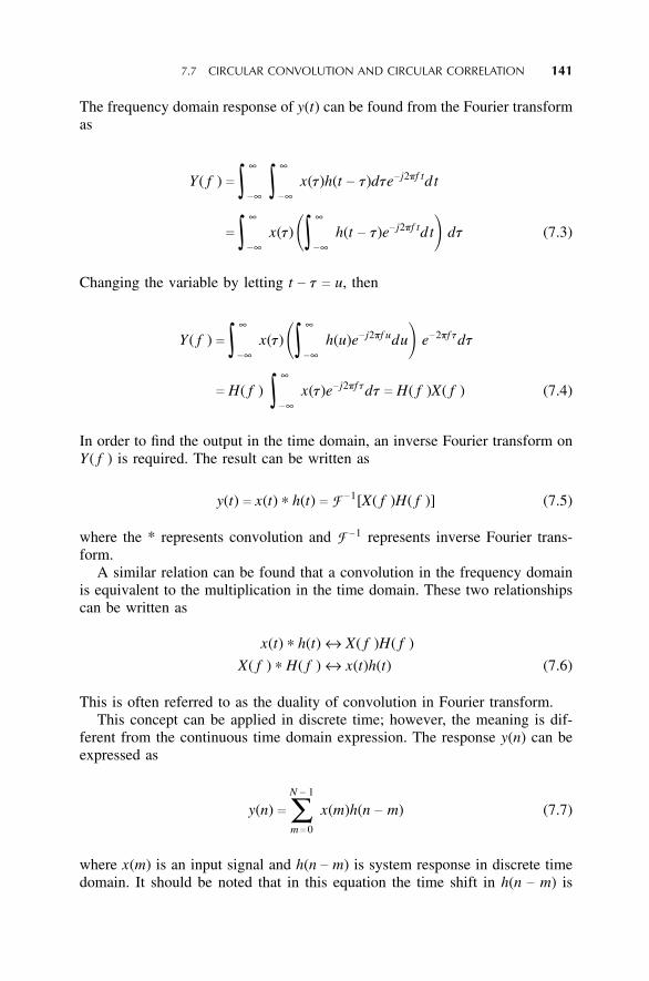
The frequency domain response of y(t) can be found from the Fourier transformas

Y( f ) c ∫∞

−∞ ∫∞

−∞x(t)h(t − t)dte− j2pf td t

c ∫∞

−∞x(t) �∫

∞

−∞h(t − t)e− j2pf td t� dt (7.3)

Changing the variable by letting t − t c u, then

Y( f ) c ∫∞

−∞x(t) �∫

∞

−∞h(u)e− j2pf udu� e−2pftdt

c H( f ) ∫∞

−∞x(t)e− j2pftdt c H( f )X( f ) (7.4)

In order to find the output in the time domain, an inverse Fourier transform onY( f ) is required. The result can be written as

y(t) c x(t) ∗ h(t) c F −1[X( f )H( f )] (7.5)

where the * represents convolution and F −1 represents inverse Fourier trans-form.

A similar relation can be found that a convolution in the frequency domainis equivalent to the multiplication in the time domain. These two relationshipscan be written as

x(t) ∗ h(t) ↔ X( f )H( f )

X( f ) ∗ H( f ) ↔ x(t)h(t) (7.6)

This is often referred to as the duality of convolution in Fourier transform.This concept can be applied in discrete time; however, the meaning is dif-

ferent from the continuous time domain expression. The response y(n) can beexpressed as

y(n) cN − 1

∑m c 0

x(m)h(n − m) (7.7)

where x(m) is an input signal and h(n − m) is system response in discrete timedomain. It should be noted that in this equation the time shift in h(n − m) is


circular because the discrete operation is periodic. By taking the DFT of theabove equation the result is

Y(k) cN − 1

∑n c 0

N − 1

∑m c 0

x(m)h(n − m)e(− j2pkn)/ N

cN − 1

∑m c 0

x(m) [ N − 1

∑n c 0

h(n − m)e(− j2p(n − m)k)/ N] e(− j2pmk)/ N

c H(k)N − 1

∑m c 0

x(m)e(− j2pmk)/ N c X(k)H(k) (7.8)

Equations (7.7) and (7.8) are often referred to as the periodic convolution (orcircular convolution). It does not produce the expected result of a linear con-volution. A simple argument can illustrate this point. If the input signal and theimpulse response of the linear system both have N data points, from a linearconvolution, the output should be 2N − 1 points. However, using Equation (7.8)one can easily see that the outputs have only N points. This is from the periodicnature of the DFT.

The acquisition algorithm does not use convolution; it uses correlation,which is different from convolution. A correlation between x(n) and h(n) canbe written as

z(n) cN − 1

∑m c 0

x(m)h(n + m) (7.9)

The only difference between this equation and Equation (7.7) is the sign beforeindex m in h(n + m). The h(n) is not the impulse response of a linear systembut another signal. If the DFT is performed on z(n) the result is

Z(k) cN − 1

∑n c 0

N − 1

∑m c 0

x(m)h(n + m)e(− j2pkn)/ N

cN − 1

∑m c 0

x(m) [ N − 1

∑n c 0

h(n + m)e(− j2p(n + m)k)/ N] e( j2pmk)/ N

c H(k)N − 1

∑m c 0

x(m)e( j2pmk)/ N c H(k)X−1(k) (7.10)

7.8 ACQUISITION BY CIRCULAR CORRELATION 143

where X−1(k) represents the inverse DFT. The above equation can also bewritten as

Z(k) cN − 1

∑n c 0

N − 1

∑m c 0

x(n + m)h(m)e(− j2pkn)/ N c H−1(k)X(k) (7.11)

If the x(n) is real, x(n)* c x(n) where * is the complex conjugate. Using thisrelation, the magnitude of Z(k) can be written as

|Z(k) | c |H*(k)X(k) | c |H(k)X *(k) | (7.12)

This relationship can be used to find the correlation of the input signal and thelocally generated signal. As discussed before, the above equation provides aperiodic (or circular) correlation and this is the desired procedure.

7.8 ACQUISITION BY CIRCULAR CORRELATION(2)

The circular correlation method can be used for acquisition and the method issuitable for a software receiver approach. The basic idea is similar to the dis-cussion in Section 7.6; however, the input data do not arrive in a continuousmanner. This operation is suitable for a block of data. The input data are sam-pled with a 5 MHz ADC and stored in memory. Only 1 ms of the input data areused to find the beginning point of the C/ A code and the searching frequencyresolution is 1 KHz.

To perform the acquisition on the input data, the following steps are taken.

1. Perform the FFT on the 1 ms of input data x(n) and convert the input intofrequency domain as X(k) where n c k c 0 to 4999 for 1 ms of data.

2. Take the complex conjugate X(k) and the outputs become X(k)*.3. Generate 21 local codes lsi(n) where i c 1, 2, . . . 21, using Equation (7.1).

The local code consists of the multiplication of the C/ A code satellite sand a complex RF signal and it must be also sampled at 5 MHz. Thefrequency f i of the local codes are separated by 1 KHz.

4. Perform FFT on lsi(n) to transform them to the frequency domain as Lsi(k).5. Multiply X(k)* and Lsi(k) point by point and call the result Rsi(k).6. Take the inverse FFT of Rsi(k) to transform the result into time domain

as rsi(n) and find the absolute value of the |rsi(n) | . There are a total of105,000 (21 × 5,000) of |rsi(n) | .

7. The maximum of |rsi(n) | in the nth location and ith frequency bin givesthe beginning point of C/ A code in 200 ns resolution in the input dataand the carrier frequency in 1 KHz resolution.


FIGURE 7.4 Illustration of acquisition with periodic correlation.

The above operation can be represented in Figure 7.4. The result shown in thisfigure is in the time domain and only one of the 21 local codes is shown. One canconsider that the input data and the local data are on the surfaces of the two cylin-ders. The local data is rotated 5,000 times to match the input data. In other words,one cylinder rotates against the other one. At each step, all 5,000 input data aremultiplied by the 5,000 local data point by point and results are summed together.It takes 5,000 steps to cover all the possible combinations of the input and the localcode. The highest amplitude will be recorded. There are 21 pairs of cylinders (notshown). The highest amplitude from the 21 different frequency components is thedesired value, if it also crosses a certain threshold.

Computer program (p7 1) will show the above operation with fine frequencyinformation in Section 7.13. The determination and setting a specific thresholdare not included in this program, but the results are plotted in time and fre-quency domain. One can determine the results from the plots.

7.9 MODIFIED ACQUISITION BY CIRCULAR CORRELATION(4)

This method is the same as the one above. The only difference is that the lengthof the FFT is reduced to half. In step 3 of the circular correlation method inthe previous section the local code lsi(n) is generated. Since the lsi(n) is a com-plex quantity, the spectrum is asymmetrical as shown in Figure 7.5. From thisfigure it is obvious that the information is contained in the first-half spectrumlines. The second-half spectrum lines contain very little information. Thus theacquisition through the circular correlation method can be modified as follows:

7.9 MODIFIED ACQUISITION BY CIRCULAR CORRELATION 145

FIGURE 7.5 Spectrum of the locally generated signal.

1. Perform the FFT on the 1 ms of input data x(n) and convert the input intofrequency domain as X(k) where n c k c 0 to 4,999 for 1 ms of data.

2. Use the first 2,500 X(k) for k c 0 to 2,499. Take the complex conjugateand the outputs become X(k)*.

3. Generate 21 local codes lsi(n) where i c 1, 2, . . . 21, using Equation (7.1)as discussed in the previous section. Each lsi(n) has 5,000 points.

4. Perform the FFT on lsi(n) to transform them to the frequency domain asLsi(k).

5. Take the first half of Lsi(k), since the second half of Lsi(k) contains verylittle information. Multiply Lsi(k) and X(k)* point by point and call theresult Rsi(k) where k c 0 ∼ 2499.

6. Take the inverse FFT of Rsi(k) to transform the result back into timedomain as rsi(n) and find the absolute value of the |rsi(n) | . There are atotal of 52,500 (21 × 2,500) of |rsi(n) | .

7. The maximum of |rsi(n) | is the desired result, if it is also above a pre-determined threshold. The ith frequency gives the carrier frequency witha resolution of 1 KHz and the nth location gives the beginning point ofC/ A code with a 400 ns time resolution.

8. Since the time resolution of the beginning of the C/ A code with this


method is 400 ns, the resolution can be improved to 200 ns by comparingthe amplitudes of nth location with (n − 1) and (n + 1) locations.

In this approach from steps 5 through 7 only 2,500 point operations are per-formed instead of the 5,000 points. The sorting process in step 7 is simplerbecause only half the outputs are used. Step 8 is very simple. Therefore, thisapproach saves operation time. Simulated results show that this method hasslightly lower signal-to-noise ratio, about 1.1 dB less than the regular circularcorrection method. This might be caused by the signal loss in the other half ofthe frequency domain.

7.10 DELAY AND MULTIPLY APPROACH(3–5)

The main purpose of this method is to eliminate the frequency information in theinput signal. Without the frequency information one need only use the C/ A codeto find the initial point of the C/ A code. Once the C/ A is found, the frequencycan be found from either FFT or DFT. This method is very interesting froma theoretical point of view; however, the actual application for processing theGPS signal still needs further study. This method is discussed as follows. Firstlet us assume that the input signal s(t) is complex, thus

s(t) c Cs(t)ej2pf t (7.13)

where Cs(t) represents the C/ A code of satellite s. The delayed version of thissignal can be written as

s(t − t) c Cs(t − t)e j2pf (t − t) (7.14)

where t is the delay time. The product of s(t) and the complex conjugate ofthe delayed version s(t − t) is

s(t)s(t − t)* c Cs(t)Cs(t − t)*e j2pf te − j2pf (t − t) ≡ Cn(t)ej2pft (7.15)

where

Cn(t) ≡ Cs(t)Cs(t − t) (7.16)

can be considered as a “new code,” which is the product of a Gold code and itsdelayed version. This new “new code” belongs to the same family as the Goldcode.(5) Simulated results show that its autocorrelation and the cross correlationcan be used to find its beginning point of the “new code.” The beginning pointof the “new code” is the same as the beginning point of the C/ A code. The

7.10 DELAY AND MULTIPLY APPROACH 147

interesting thing about Equation (7.15) is that it is frequency independent. Theterm e j2pft is a constant, because f and t are both constant. The amplitude ofej2pft is unity. Thus, one only needs to search for the initial point of the “newcode.” Although this approach looks very attractive, the input signal must becomplex. Since the input data collected are real, they must be converted to com-plex. This operation can be achieved through the Hilbert transform discussedin Section 6.13; however, additional calculations are required.

A slight modification of the above method can be used for a real signal.(4)

The approach is as follows. The input signal is

s(t) c Cs(t) sin(2pf t) (7.17)

where Cs(t) represents the C/ A code of satellite s. The delayed version of thesignal can be written as

s(t − t) c Cs(t − t) sin[2pf (t − t)] (7.18)

The product of s(t) and the delayed signal s(t − t) is

s(t)s(t − t) c Cs(t)Cs(t − t) sin(2pf t) sin[2pf (t − t)]

≡Cn(t)

2{cos(2pft) − cos[2pf (2t − t)]} (7.19)

where Cn(t) is defined in Equation (7.16). In the above equation there are twoterms: a dc term and a high-frequency term. Usually the high frequency canbe filtered out. In order to make this equation usable, the | cos(2pft) | must beclose to unity. Theoretically, this is difficult to achieve, because the frequencyf is unknown. However, since the frequency is within 1250 ± 10 KHz, it ispossible to select a delay time to fulfill the requirement. For example, one canchose 2 × p × 1,250 × 103t c p, thus, t c 0.4 × 10−6 s c 400 ns. Since theinput data are digitized at 5 MHz, the sampling time is 200 ns (1/ 5 MHz). Ifthe input signal is delayed by two samples, the delay time t c 400 ns. Underthis condition | cos(2pft) | c | cos(p) | c 1. If the frequency is off by 10 KHz,the corresponding value of | cos(2pft) | c | cos(2p × 1,260 × 103 × 0.4 × 10−6) |c 0.9997, which is close to unity. Therefore, this approach can be applied toreal data. The only restriction is that the delay time cannot be arbitrarily chosenas in Equation (7.15). Other delay times can also be used. For example, delaytimes of a multiple of 0.4 us can be used, if the delay line is not too long. Forexample, if t c 1.6 us, when the frequency is off by ±10 KHz, the | cos(2pft) |c 0.995. One can see that | cos(2pft) | decreases faster if a long delay time isused for a frequency off the center value of 1,250 KHz. If the delay time is toolong the | cos(2pft) | may no longer be close to unity.

The problem with this approach is that when two signals with noise are mul-tiplied together the noise floor increases. Because of this problem one cannot


FIGURE 7.6 Effect of phase transition on the delay and multiplication method.

search for 1 ms of data to acquire a satellite. Longer data are needed for acquir-ing a certain satellite.

One interesting point is that a navigation data change does not have a sig-nificant effect on the correlation result. Figure 7.6 shows this result. In Figure7.6a there is no phase shift due to navigation data. The “new code” createdby the multiplication of the C/ A code and its delayed version will be repeti-tive every millisecond as the original C/ A code. If there are two phase shiftsby the navigation data, the only regions where the original C/ A code and thedelayed C/ A code have a different code are shown in Figure 7.6b. The rest ofthe regions generate the same “new code.” If there are 5,000 data points perC/ A code, delaying two data points only degrades the performance by 2/ 5,000,caused by a navigation transition. Therefore, using this acquisition method onedoes not need to check for two consecutive data sets to guarantee that thereis no phase shift by the navigation data in one of the sets. One can choose alonger data record and the result will improve the correlation output.

Experimental results indicate that 1 ms of data are not enough to find anysatellite. The minimum data length appears to be 5 ms. Sometimes, one singledelay time of 400 ns is not enough to find a desired signal. It may take severaldelay times, such as 0.4, 0.8, and 1.2 us, together to find the signals. A fewweak signals that can be found by the circular correlation method cannot befound by this delay and multiplication method. With limited results, it appearsthat this method is not suitable to find weak signals.

7.11 NONCOHERENT INTEGRATION 149

7.11 NONCOHERENT INTEGRATION

Sometimes using 1 ms of data through the circular correlation method cannotdetect a weak signal. Longer data records are needed to acquire a weak signal.As mentioned in Sections 7.4 and 7.5, an increase in the data length can requiremany more operations. One way to process more data is through noncoherentintegration. For example, if 2 ms of data are used, the data can be divided intotwo 1 ms blocks. Each 1 ms of data are processed separately and the results aresummed together. This operation basically doubles the number of operations,except for the addition in the last stage. In this operation, the signal strengthis increased by a factor of 2 but the noise is increased by a factor of

f2,

thus, the signal-to-noise ratio increases byf

2 (or 1.5 dB). The improvementobtained by this method is less than with the coherent method but there arefewer operations.

Another advantage of this latter method is the ability to keep performingacquisition on successive 1 ms of data and summing the results. The finalresult can be compared with a certain threshold. Whenever the result crossesthe threshold, the signal is found. A maximum data length can be chosen. Ifa signal cannot be found within the maximum data length, this process willautomatically stop. Using this approach, strong signals can be found from 1ms of data, but weak signals will take a longer data length. If there is phaseshift caused by the navigation data, only the 1 ms of data with the phase shiftwill be affected. Therefore, the phase shift will have minimum impact on thisapproach. Conventional hardware receivers often use this approach.

7.12 COHERENT PROCESSING OF A LONG RECORD OF DATA(6)

This section presents the concept of processing a long record of data coher-ently with fewer operations. The details are easy to implement, thus they willnot be included. The common approach to find a weak signal is to increase theacquisition data length. The advantage of this approach is the improvement insignal-to-noise ratio. One simple explanation is that an FFT with 2 ms of dataproduces a frequency resolution of 500 Hz in comparison with 1 KHz resolutionof 1 ms of data. Since the signal is narrow band after the spectrum despread, thesignal strength does not reduce by the narrower frequency resolution. Reducingthe resolution bandwidth reduces the noise to half; therefore, the signal-to-noiseratio improves by 3 dB. If 10 ms of data are to be processed, the circular cor-relation method may not be practical because of the computational complexityas discussed in Section 7.5.

The idea here is to perform FFT with fewer points. Let us use 10 ms of data(or 50,000 points) as an example to illustrate the idea. The center frequency ofdata is at 1.25 MHz. If one multiplies these data with a complex cw signal of1.25 MHz, the input signal will be converted into a baseband and a high-fre-quency band at 2.5 MHz. If the high-frequency component is filtered out, only


the baseband signal will be processed. Let us assume that the high frequencysignal is filtered out. The baseband signal is a down-converted version of theinput with the C/ A code. One can multiply this signal by the C/ A code pointby point. If the correct phase of the C/ A code is achieved, the output is a cwsignal and the maximum frequency range is ±10 KHz, caused by the Dopplerfrequency shift. Since the bandwidth of this signal is 20 KHz, one can samplethis signal at 50 KHz, which is 2.5 times the bandwidth. With this samplingfrequency there are only 500 data points in 10 ms. However, the signal is sam-pled at 5 MHz and there are 50,000 data points. One can average 100 pointsto make one data point. This averaging is equivalent to a low-pass filter; there-fore, it eliminates the high-frequency components created by the multiplicationof the 1.25 MHz cw signal as well as noise in the collected signal. Since thedata are 10 ms long, the frequency resolution from the FFT is 100 Hz.

This approach is stated as follows by using 10 ms of data as an example:

1. Multiply 10 ms of the input signal by a locally generated complex cwsignal at 1.25 MHz and digitized at 5 MHz. Let us refer to this outputas the low-frequency output because the maximum frequency is 10 KHz.The high-frequency components at about 2.5 MHz will be filtered outlater, thus, they will be neglected in this discussion. A total of 50,000points of data will be obtained.

2. Multiply these output data by the desired 10 C/ A codes point by pointto obtain a total of 50,000 points.

3. Average 100 adjacent points into one point. This process filters out thehigh frequency at approximately 2.5 MHz.

4. Perform 500-point FFT to find a high output in the frequency domain.This operation generates only 250 useful frequency outputs.

5. Shift one data point of local code with respect to the low-frequency outputand repeat steps 3 and 4. Since the C/ A repeats every ms, one needs toperform this operation 5,000 times instead of 50,000 times.

6. There are overall 1.25 × 106 (250 × 5,000) outputs in the frequencydomain. The highest amplitude that crosses a certain threshold will bethe desired value. From this value the beginning of the C/ A code and theDoppler frequency can be obtained. The frequency resolution obtained is100 Hz.

Although the straightforward approach is presented above, circular correla-tion can be used to achieve the same purpose with fewer operations.

7.13 BASIC CONCEPT OF FINE FREQUENCY ESTIMATION(7)

The frequency resolution obtained from the 1 ms of data is about 1 KHz, whichis too coarse for the tracking loop. The desired frequency resolution should be

7.14 RESOLVING AMBIGUITY IN FINE FREQUENCY MEASUREMENTS 151

within a few tens of Hertz. Usually, the tracking loop has a width of only afew Hertz. Using the DFT (or FFT) to find fine frequency is not an appropriateapproach, because in order to find 10 Hz resolution, a data record of 100 ms isrequired. If there are 5,000 data points/ ms, 100 ms contains 500,000 data points,which is very time consuming for FFT operation. Besides, the probability ofhaving phase shift in 100 ms of data is relatively high.

The approach to find the fine frequency resolution is through phase relation.Once the C/ A code is stripped from the input signal, the input becomes a cwsignal. If the highest frequency component in 1 ms of data at time m is Xm(k), krepresents the frequency component of the input signal. The initial phase vm(k)of the input can be found from the DFT outputs as

vm(k) c tan−1 � Im(Xm(k))Re(Xm(k)) � (7.20)

where Im and Re represent the imaginary and real parts, respectively. Let usassume that at time n, a short time after m, the DFT component Xn(k) of 1 msof data is also the strongest component, because the input frequency will notchange that rapidly during a short time. The initial phase angle of the inputsignal at time n and frequency component k is

vn(k) c tan−1 � Im(Xn(k))Re(Xn(k)) � (7.21)

These two phase angles can be used to find the fine frequency as

f c vn(k) − vm(k)2p(n − m)

(7.22)

This equation provides a much finer frequency resolution than the resultobtained from DFT. In order to keep the frequency unambiguous, the phasedifference vn − vm must be less than 2p. If the phase difference is at the maxi-mum value of 2p, the unambiguous bandwidth is 1/ (n − m) where n − m is thedelay time between two consecutive data sets.

7.14 RESOLVING AMBIGUITY IN FINE FREQUENCY MEASUREMENTS

Although the basic approach to find the fine frequency is based on Equation(7.22), there are several slightly different ways to apply it. If one takes the kthfrequency component of the DFT every millisecond, the frequency resolutionis 1 KHz and the unambiguous bandwidth is also 1 KHz. In Figure 7.7a fivefrequency components are shown and they are separated by 1 KHz. If the input


FIGURE 7.7 Ambiguous ranges in frequency domain.

signal falls into the region between two frequency components as shown inFigure 7.7b, the phase may have uncertainty due to noise in the system.

One approach to eliminate the uncertainty is to speed up the DFT operation.If the DFT is performed every 0.5 ms, the unambiguous bandwidth is 2 KHz.With a frequency resolution of 1 KHz and an unambiguous bandwidth of 2KHz, there will be no ambiguity problem in determining the fine frequency.However, this approach will double the DFT operations.

The second approach is to use an amplitude comparison scheme without dou-bling the speed of the DFT operations, if the input is a cw signal. As shown inFigure 7.7b, the input signal falls in between two frequency bins. Suppose thatthe amplitude of X(k) is slightly higher than X(k − 1); then X(k) will be usedin Equations (7.21) and (7.22) to find the fine frequency resolution. The differ-ence frequency should be close to 500 Hz. The correct result is that the inputfrequency is about 500 Hz lower than X(k). Due to noise the 500 Hz could beassessed as higher than X(k); therefore, a wrong answer can be reached. How-ever, for this input frequency the amplitudes of X(k) and X(k − 1) are closetogether and they are much stronger than X(k + 1). Thus, if the highest-fre-quency bin is X(k) and the phase calculated is in the ambiguous range, which isclose to the centers between X(k − 1) and X(k) or between X(k) and X(k +1), theamplitude of X(k − 1) and X(k +1) will be compared. If X(k − 1) is stronger than


FIGURE 7.8 Phase difference of less than 2p/ 5 will not cause frequency error.

X(k + 1), the input frequency is lower than X(k); otherwise, the input frequencyis higher than X(k). Under this condition, the accuracy of fine frequency isdetermined by the phase but the sign of the difference frequency is determinedby the amplitudes of two frequency components adjacent to the highest one.

However, the problem is a little more complicated than this, because it ispossible that there is a 180-degree phase shift between two consecutive datasets due to navigation data. If this condition occurs, the input can no longer betreated as a cw signal. This possibility limits the ambiguous bandwidth to 250Hz for 1 ms time delay. If the frequency is off by ±250 Hz, the correspondingangle is ±p/ 2. If the frequency is off by +250 Hz, the angle should be +p/ 2.However, a p phase shift due to the navigation will change the angle to −p/ 2(+p/ 2 − p), which corresponds to a −250 KHz change. If the phase transitionis not taken account of in finding the fine frequency, the result will be off by500 KHz.

In order to avoid this problem, the maximum frequency uncertainty must beless than 250 Hz. If the maximum frequency difference is ±200 Hz, which isselected experimentally, the corresponding phase angle difference is ±2p/ 5 asshown in Figure 7.8. If there is a p phase shift, the magnitude of the phase differ-ence is 3p/ 5 [| ±(2p/ 5)

±p | ], which is greater than 2p/ 5. From this arrangement,

the phase difference can be used to determine the fine frequency without cre-ating erroneous frequency shift. If the phase difference is greater than 2p/ 5, pcan be subtracted from the result to keep the phase difference less than 2p/ 5. In


FIGURE 7.9 Difference angle obtained from two angles.

order to keep the frequency within 200 KHz, the maximum separation betweenthe k values in X(k) will be 400 KHz. If the input is in the middle of twoadjacent k values, the input signal is 200 KHz from both of the k values. Inthe following discussion, let us keep the maximum phase difference at 2p/ 5,which corresponds to a frequency difference of 200 KHz.

The last point to be discussed is converting the real and imaginary partsof X(k) into an angle. Usually, the phase angle measured is between ±p. Thetwo angles in Equations (7.20) and (7.21) will be obtained in this manner. Thedifference angle between the two angles can be any value between 0 and 2pas shown in Figure 7.9. Since the maximum allowable difference angle is 2p/ 5for 200 KHz, the difference angle must be equal or less than 2p/ 5. If the resultis greater than 2p/ 5, 2p can be either added or subtracted from the result, andthe absolute value of the angle must be less than 2p/ 5. If noise is taken intoconsideration, the 2p/ 5 threshold can be extended slightly, such as using 2.3p/ 5,which means the difference must be equal to or less than this value. If the finalvalue of the adjusted phase difference is still greater than this threshold, it meansthat there is a phase shift between the two milliseconds of data and p shouldbe subtracted from the result. Of course, the final angle should also be adjustedby adding or subtracting 2p to obtain the final result of less than the threshold.


From the above discussion, the following steps are required to find the begin-ning of the C/ A code and the carrier frequency of a certain satellite:

1. Perform circular correlation on 1 ms of data; the starting point of a certainC/ A code can be found in these data and the carrier frequency can befound in 1 KHz resolution.

2. From the highest-frequency component X(k), perform two DFT opera-tions on the same 1 ms of data: one is 400 KHz lower and the other oneis 400 KHz higher than k in X(k). The highest output from the three out-puts [X(k − 1), X(k), X(k + 1)] will be designated to be the new X(k) andused as the DFT component to find the fine frequency.

3. Arbitrarily choose five milliseconds of consecutive data starting from thebeginning of the C/ A code. Multiply these data with 5 consecutive C/ Acodes; the result should be a cw signal of 5 ms long. However, it mightcontain one p phase shift between any of the 1 ms of data.

4. Find Xn(k) on all the input data, where n c 1, 2, 3, 4, and 5. Then find thephase angle from Equation (7.20). The difference angle can be defined as

Dv c vn + 1 − vn (7.23)

5. The absolute value of the difference angle must be less than the threshold(2.3p/ 5). If this condition is not fulfilled, 2p can be added or subtractedfrom Dv . If the result is still above the threshold, p can be added or sub-tracted from Dv to adjust for the p phase shift. This result will also betested against the 2.3p/ 5 threshold. If the angle is higher than the thresh-old, 2p can be added or subtracted to obtain the desired result. After theseadjustments, the final angle is the desired value.

6. Equation (7.22) can be used to find the fine frequency. Since there are5 ms of data, there will be 4 sets of fine frequencies. The average valueof these four fine frequencies will be used as the desired fine frequencyvalue to improve accuracy.

Program (p7 1) listed at the end of this chapter can be used to find theinitial point of the C/ A code as well as the fine frequency. This program callsthe digitizg.m, which generates digitized C/ A code. The digitizg.m in turn callscodegen.m, which is a modified version of program (p5 2), and generates theC/ A code of the satellites. These programs just provide the basic idea. They canbe modified to solve certain problems. For example, one can add a thresholdto the detection of a certain satellite. If the signal is weak, one can use severalmilliseconds of data and add them incoherently.


7.15 AN EXAMPLE OF ACQUISITION

In this section the acquisition computer program (p7 1) is used to find the ini-tial point of a C/ A code and the fine frequency. The computer program willoperate on actual data collected. The experimental setup to collect the data issimilar to Figure 6.5b. The data were digitized at 5 MHz. The data contain 7satellites, numbers 6, 10, 17, 23, 24, 26, and 28. Most of the satellites in thedata are reasonably strong and they can be found from 1 ms of data. However,this is a qualitative discussion, because no threshold is used to determine theprobability of detection. Satellite 24 is weak; in order to confirm this signalseveral milliseconds of data need to be added incoherently.

The input data in the time domain are shown in Figure 7.10. As expected, thedata look like noise. The frequency plot of the input can be found through theFFT operation as shown in Figure 7.11. The bandwidth is 2.5 MHz as expected.The spectrum shape resembles the shape of the filter in the RF chain. After thecircular correlation, the beginning of the C/ A code of satellite 6 is shown inFigure 7.12. The beginning of the C/ A code is at 2884. The amplitudes of the21 frequency components separated by 1 KHz are shown in Figure 7.13. Thehighest component occurs at k c 7. From Figures 7.12 and 7.13, one can see that

FIGURE 7.10 Input data.

7.15 AN EXAMPLE OF ACQUISITION 157

FIGURE 7.11 FFT of input data.

FIGURE 7.12 Beginning of C/ A code of satellite 6.


FIGURE 7.13 Frequency component of the despread signal of satellite 6.

the initial point of the C/ A code and the frequency are clearly shown. Sincethe data are actually collected, the accuracy of the fine frequency is difficultto determine because the Doppler frequency is unknown. The fine frequencyalso depends on the frequency accuracy of the local oscillator used in the downconversion and the accuracy of the sampling frequency.

One way to get a feeling of the calculated fine frequency accuracy is touse different portions of the data. Six fine frequencies are calculated from dif-ferent portions of the input data. The data used are 1–25000, 5001–30001,10001–35001, 15001–40001, 20001–45001, 25001–50001. These data are fivemilliseconds long and the starting points are shifted by 1 ms. Between two adja-cent data sets four out of the five milliseconds of data are the same. Therefore,the calculated fine frequency should be close. The fine frequency differencesbetween these six sets are −2.4, 9.0, −8.2, 5.4, and 2.3 Hz. These data are col-lected at a stationary set. The frequency change per millisecond should be verysmall as discussed in Chapter 3. Thus, the frequency difference can be con-sidered as the inaccuracy of the acquisition method. When the signal strengthchanges, the difference of the fine frequency also changes. For a weak signalthe frequency difference can be in tens of Hertz, if the same calculation methodis used.

7.16 SUMMARY 159

FIGURE 7.14 Beginning of C/ A code of satellite 24.

The acquisition performed on a weak signal (satellite 24) is shown in Figures7.14 and 7.15. From these figures, it is difficult to assess whether the beginningpoint of the C/ A code and the frequency are the correct values. The beginningof the C/ A code and the fine frequency can be found by adding more calcula-tions incoherently. The correct results are different from the maximum shownin Figures 7.14 and 7.15.

7.16 SUMMARY

The concept of signal acquisition is discussed in this section. The circular corre-lation method can provide fast acquisition without sacrificing detection sensitiv-ity. Although there are methods that can operate at a faster speed than the circu-lar correlation method, they usually have lower detection sensitivity. It appearsthat the circular correction method using 1 ms of data is able to acquire signalsfrom most satellites. The delay and multiplication method must use more than1 ms of data to acquire a signal because of the high noise level created. Theacquisition provides the beginning of the C/ A code and a coarse frequency. Thefine frequency can be found through phase comparison to within a few tens of


FIGURE 7.15 Frequency component of the despread signal of satellite 24.

Hertz. To speed up the operation of the acquisition process is always desirablein software GPS receivers.

REFERENCES

1. Oppenheim, A. V., Schafer, R. W., Digital Signal Processing, Prentice-Hall, Engle-wood Cliffs, NJ, 1975.

2. Van Nee, D. J. R., Coenen, A. J. R. M., “New fast GPS code acquisition techniqueusing FFT,” Electronics Letters, vol. 27, pp. 158–160, January 17, 1991.

3. Tomlinson, M., School of Electronic, Communication and Electrical Engineering,University of Plymouth, United Kingdom, private communication.

4. Lin, D., Tsui, J., “Acquisition schemes for software GPS receiver,” ION GPS-98,pp. 317–325, Nashville, TN, September 15–18, 1998.

5. Wolfert, R., Chen, S., Kohli, S., Leimer, D., Lascody, J., “Rapid direct P(Y)-codeacquisition in a hostile environment,” ION GPS-98, pp. 353–360, Nashville, TN,September 15–18, 1998.

6. Spilker, J. J., “GPS signal structure and performance characteristics,” Navigation,Institute of Navigation, vol. 25, no. 2, pp. 121–146, Summer 1978.

7. Tsui, J. B. Y., Digital Techniques for Wideband Receivers, Artech House, Boston,1995.

REFERENCES 161

% p7 1.m performs acquisition on collected data

clear

% ***** initial condition *****

svnumcinput(’enter satellite number c ’);intodatc10001; %input(’enter initial pt into data (multiple of n) c’);fsc5e6; % *** sampling freqtsc1/fs; % *** sampling timencfs/1000; % *** data pt in 1 msnnc[0:n-1]; % *** total no. of ptsfcc1.25e6; % *** center freq without Dopplernsatclength(svnum); % *** total number of satellites to be processed

% ***** input data file *****

fidcfopen(’d:/gps/Big data/srvy1sf1.dat’, ’r’);fseek(fid,intodat-1, ’bof’);x2cfread(fid,6*n, ’schar’);

yy c zeros(21,n);

% ***** start acquisition *****

codecdigitizg(n,fs,0,svnum); % digitize C/A codexf c fft(x2(1:n)’);for i c [1:21]; % *** find coarse freq 1 KHz resolution

frcfc-10000+(i-1)*1000;lcccode.* exp(j*2*pi*fr*ts*nn); % generate local codelcfcfft(lc);yy(i,:)cifft(xf .* conj(lcf)); % circular correlation

end[amp crw]cmax(max(abs(yy’))); % find highest peak[amp ccn]cmax(max(abs(yy)));

pt initcccn; % initial pointcfrqcfc+1000*(crw-11); % coarse freq

% ***** gerenate 5 ms data by stripping C/A code *****

z5cx2(pt init:pt init+5*n-1); % take 5 ms data starting with C/A codeza5cz5’ .* [code code code code code];% create cw from 5 sets of data


% ***** find medium freq resolution 400 KHz apart *****

for i c [1:3];frccfrq-400+(i-1)*400;mfrq0(i)csum(za5(1:5000) .* exp(j*2*pi*fr*ts*nn));mfrq1(i)cabs(mfrq0(i));

end[mamp mrw] c max(mfrq1); % find highest peakmfrqccfrq+200*(mrw-2);frcmfrq; % medium freq

% ***** find fine freq *****

zb5cza5 .* exp(j*2*pi*fr*ts*[0:5*n-1]); % one DFT componentzc5cdiff(-angle(sum(reshape(zb5,n,5)))); % find difference anglezc5fixczc5;

% ***** Adjust phase and take out possible phase shift *****

thresholdc2.3*pi/5;for ic1:4;

if abs(zc5(i))>threshold;% for angle adjustmentzc5(i)czc5fix(i)-2*pi;if abs(zc5(i))>threshold;

zc5(i)czc5fix(i)+2*pi; % endif abs(zc5(i))>2.2*pi/5; % for pi phase shift correction

zc5(i)czc5fix(i)-pi;if abs(zc5(i))>threshold;

zc5(i)czc5fix(i) - 3*pi;if abs(zc5(i))>threshold;

zc5(i)czc5fix(i)+pi; %endend

endend

endend

end

dfrqcmean(zc5)*1000/(2*pi);frrcfr+dfrq;% fine freq

plot(abs(yy(crw,1:n)))title([’GPS c ’ num2str(svnum)’ max at ’ num2str(pt init)])figureplot(abs(yy):,ccn)), ’*’)

REFERENCES 163

% title([’GPS c ’ num2str(svnum) ’ Freq c ’ num2str(frr)])formatpt initformat long efrr

% digitizg.m This prog generates the C/A code and digitizes itfunction code2 c digitizg(n,fs,offset,svnum);

% code - gold code% n - number of samples% fs - sample frequency in Hz;% offset - delay time in seconds must be less than 1/fs cannot shiftleft% svnum - satellite number;

gold rate c 1.023e6; %gold code clock rate in Hz.tsc1/fs;tcc1/gold rate;

cmd1 c codegen(svnum); % generate C/A codecode inccdm1;

% ***** creating 16 C/A code for digitizing *****

code a c [code in code in code in code in];code ac[code a code a];code ac[code a code a];

% ***** digitizing *****

b c [1:n];c c ceil((ts*b+offset)/tc);code c code a(c);

% ***** adjusting first data point *****

if offset>c0;code2c[code(1) code(1:n-1)];

elsecode2c[code(n) code(1:n-1)];

end

% codegen.m generates one of the 32 C/A codes written by D.Akos modifiedby J. Tsui


function [ca used]ccodegen(svnum);

% ca used : a vector containing the desired output sequence% the g2s vector holds the appropriate shift of the g2 code to generate% the C/A code (ex. for SV#19 - use a G2 shift of g2s(19)c471)% svnum: Satellite number

gs2 c [5;6;7;8;17;18;139;140;141;251;252;254;255;256;257;258;469;470;471; ... 472;473;474;509;512;513;514;515;516;859;860;861;862];

g2shiftcg2s(svnum,1);

% ***** Generate G1 code *****

% load shift registerreg c -1*ones(1,10);

for i c 1:1023,g1(i) c reg(10);save1 c reg(3)*reg(10);reg(1,2:10) c reg(1:1:9);reg(1) c save1;

end,

% ***** Generate G2 code *****% load shift register

reg c -1*ones(1,10);for i c 1:1023,

g2(i) c reg(10);save2 c reg(2)*reg(3)*reg(6)*reg(8)*reg(9)*reg(10);reg(1,2:10) c reg(1:1:9);reg(1) c save2;

end

% ***** Shift G2 code *****g2tmp(1,1:g2shift)cg2(1,1023-g2shift+1:1023);g2tmp(1,g2shift+1:1023)cg2(1,1:1023-g2shift);g2 c g2tmp;

% ***** Form single sample C/A code by multiplying G1 and G2

ss ca c g1.*g2;ca usedc-ss ca;

Date post:	19-Jul-2018
Category:	Documents
Upload:	vuongngoc
View:	213 times
Download:	0 times

Acquisition of GPS CA Code Signals - pudn.comread.pudn.com/downloads85/ebook/326017/Fundamentals of...

Documents