146
ISSN 1220-8434 Volume 18, 2010
| Date post: | 30-Sep-2014 |
| Category: |
Documents |
| Upload: | ciotea-mariana |
| View: | 32 times |
| Download: | 1 times |

ISSN 1220-8434 Volume 18, 2010


ACTA TRIBOLOGICA
Volume 18, 2010


Acta tribologicaA Journal on the Science of Contact Mechanics, Friction, Lubrication,
Wear, Micro/Nano Tribology, and Biotribology
Volume 18, 2010
EDITOR E. Diaconescu, University of Suceava, ROMANIA
EDITORIAL BOARD N.N. Antonescu, Petroleum-Gas University of Ploiesti, ROMANIAJ.R. Barber, University of Michigan, U.S.AY. Berthier, INSA de Lyon, FRANCEM. Ciavarella, Politecnico di Bari, ITALYT. Cicone, University Politehnica of Bucharest, ROMANIAS. Cretu, Technical University of Iasi, ROMANIAL. Deleanu, University of Galati, ROMANIAD. Dini, Imperial College London, UNITED KINGDOMV. Dulgheru, Technical University of Moldova, MOLDOVAI. Etsion, Technion, Haifa, ISRAELM. Glovnea, University of Suceava, ROMANIAR. Glovnea, University of Sussex, UNITED KINGDOMI. Green, Georgia Institute of Technology, U.S.AM. Khonsari, Louisiana State University, U.S.AY. Kligerman, Technion, Haifa, ISRAELD. Nelias, INSA de Lyon, FRANCED. Olaru, Technical University of Iasi, ROMANIAM. Pascovici, University Politehnica of Bucharest, ROMANIAM. Ripa, University of Galati, ROMANIAA. Tudor, University Politehnica of Bucharest, ROMANIA
ASSISTANT EDITOR S. Spinu, University of Suceava, ROMANIA

Published by the Applied Mechanics Section of the University of Suceava
University “Stefan cel Mare” of Suceava Publishing House
13th University Street, Suceava, 720229, Suceava, ROMANIAPhone: (40) – 0230 – 216 – 147 int. 273, E-mail: [email protected]

ACTA TRIBOLOGICA VOLUME 18, 2010
CONTENTS
1 A. URZICĂ, S. CRETU A Numerical Procedure to Generate Non-Gaussian Rough Surfaces
7 C. CIORNEI, E. DIACONESCUPreliminary Theoretical Solution for Electric Contact Resistance betweenRough Surfaces
12 C.-I. BARBINTA, S. CRETUThe Influence of the Rail Inclination and Lateral Shift on Pressure Distributionin Wheel - Rail Contact
19 C. SUCIU, E. DIACONESCUPreliminary Theoretical Results upon Contact Pressure Assessment by Aid ofReflectivity
27 S. SPINUNumerical Simulation of Elastic-Plastic Contact
34 Y. NAGATA, R. GLOVNEADielectric Properties of Grease Lubricants
42 J. PADGURSKAS, R. KREIVAITIS, A. KUPČINSKAS, R. RUKUIŽA, V. JANKAUSKAS, I. PROSYČEVAS Influence of Nanoparticles on Lubricity of Base Mineral Oil
46 A.V. RADULESCU, I. RADULESCUInfluence of the Rheometer Geometry on the Rheological Properties ofIndustrial Lubricants
52 V.-F. ZEGREAN, E. DIACONESCUMeasurement of Lubricant Oil Microviscosity Based on Resonant FrequencyShift of AFM Cantilever
58 M.C. CORNECI, A.-M. TRUNFIO-SFARGHIU, F. DEKKICHE, Y.BERTHIER, M.-H. MEURISSE, J.-P. RIEUInfluence of Lubricant Physicochemical Properties on the TribologicalOperation of Fluid Phase Phospholipid Biomimetic Surfaces

65 S. LE FLOC’H, M.C. CORNECI, A.-M. TRUNFIO-SFARGHIU, M.-H.MEURISSE, J.-P. RIEU, J. DUHAMEL, C. DAYOT, F. DANG, M. BOUVIER,C. GODEAU, A. SAULOT, Y. BERTHIERImagerie Medicale pour Evaluer les Conditions du FonctionnementTribologiques des Articulations Synoviales
77 M.C. CORNECI, A.-M. TRUNFIO-SFARGHIU, F. DEKKICHE,Y. BERTHIER, M.-H. MEURISSE, J.-P. RIEU, M. LAGARDE,M. GUICHARDANTPhospholipides dans le Fluid Synovial - Influence sur le FonctionnementTribologique des Articulations Synoviales Pathologiques
85 I.C. ROMANU, E. DIACONESCUBioarticular Friction
89 A.-M. TRUNFIO-SFARGHIU, M.C. CORNECI, Y. BERTHIER,M.-H. MEURISSE, J.-P. RIEUMechanical and Physicochemical Analysis of the Tribological Operation ofJoint Replacements
106 D. N. OLARU, C. STAMATE, A. DUMITRASCU, G. PRISACARURolling Friction Torque in Microsystems
113 L. DELEANU, S. CIORTANEvaluating Tribological Damages by 3D Profilometry
120 M. RÎPĂ, S. BOICIUC Characterisation of Laser Cladding with Ni–Cr–B–Fe–Al Alloy byProfilometric Study of the Scratch Tracks
128 M. VLASE, A. TUDORAn Analytical Wear Model of the Pipes for Concrete Transportation

ISSN 1220 - 8434 ACTA TRIBOLOGICA Volume 18, (2010), 1-6
Ana URZICĂ e-mail: [email protected]
Spiridon CREŢU
e-mail: [email protected]
Department of Machine Design,
Technical University of Iaşi,
ROMANIA
A NUMERICAL PROCEDURE TO GENERATE NON-GAUSSIAN ROUGH SURFACES The paper presents an algorithm for computer simulation of non-Gaussian surfaces. By using a random number generator, a input matrix is formed as a first representation of a Gaussian roughness with zero mean, and unit standard deviation. The autocorrelation function was assumed to have an exponential form. To fulfill this requirement, in the first step, the matrix containing the roughness heights was obtained by a linear transformation of the input matrix. In the second step the skewness and kurtosis of the input sequence have been established for the desired skewness and kurtosis of an output sequence. Finally the non-Gaussian random series have been generated by using the Johnson translator system. The numerical results pointed out that the developed algorithm can be further used to simulate manufacturing processes that produce real surfaces which may present a non-Gaussian distribution, as well as the abrasive wear and running in phenomena. Keywords: roughness, autocorrelation, skewness, kurtosis
1. INTRODUCTION
Both experimental and numerical studies
have pointed out that roughness acts as stress concentration sites and induce stresses greater than in an equivalent smooth contact. The real areas of contact and the asperity contact pressures are essential parameters for any wear modeling. These parameters can vary significantly depending on surface topography. A small change in the distribution of heights, wave length and curvature of the surface roughness can have a noticeable effect on the deformation behaviors of the rough surfaces.
Manufacturing processes produce real surfaces which are sometimes quite different from Gaussian distribution. For example, a lathe turned surface is far from random; its peaks are nearly all the same height and its valley nearly all the same depth. A ground surface which is subsequently polished so that the tips of the higher asperities are removed departs markedly from being Gaussian.
Figure 1. The changes in profile caused by running in and abrasive wear
Similar profiles are presented by surfaces that had carried out abrasive wear or running in processes, Figure 1.
Any parametric study involving roughness requires surfaces with known statistical proprieties and it is much more convenient to generate them numerically rather to measure manufactured rough surfaces. An essential requirement for any numerical algorithms for roughness simulation is their abilities to generate rough surface which have statistical proprieties similar to real surfaces.
Most of the statistical proprieties of a rough surface can be derived from knowledge of two statistical functions: the frequency density function and the autocorrelation function, Bakolas V. [1], Bushan B. [2], Greenwood J.A. [6], Robbe - Valloire F. [11]. J.Mc.Cool [9] shows that it is possible to describe any statistical distribution through knowledge of only four central moments of cumulative distribution function of probabilities.
Consequently, a good algorithm should be able to generate surfaces having prescribed frequency density functions and autocorrelation functions.
The developed procedure starts from the imposed values for the normalized central moments: the mean height, aR , standard deviation qR , skewness parameter Sk, kurtosis parameter K, as well as for the correlation lengths λx, λy, of the autocorrelation function.

2
2. SPATIAL AND SPECTRAL PARAMETERS OF ROUGHNESS
2.1 Probability Density Function (PDF) If for convenience z was measured from the
mean plane of the surface, then the height z(x, y) of a rough surface may be considered as a two-dimensional random variable. The spatial characteristics can be adequately described with the use of probability function p(z) which denotes the probability that a point on the surface has a height equal to z. It has been found, Bakolas V. [1], Bhushan B. [2], Patir N. [10], that many real surfaces, notably freshly grounded surfaces, reveal a height distribution which is close to the normal Gaussian probability function:
2
2σ zp(z) exp
2σ2π −
=
, (1)
where σ is the standard (r.m.s.) deviation from the mean height.
The shape of the probability function can provide useful information about the nature of the roughness profile. A mathematical presentation of this shape is provided by the moments of the probability density function about the mean. 2.2 The normalized moments of PDF
The first normalized central moment is the mean height, aR which is generally removed before data processing and is therefore zero:
aR z p(z) dz∞
−∞= ⋅ ⋅∫ . (2)
The second moment is the variance 2
qR of the roughness heights, meaning the standard deviation qR , or the root mean square (r.m.s.) σ , of the surface heights:
2 2z p(z) dz
∞
−∞σ = ⋅ ⋅∫ . (3)
The third normalized central moment is called „skewness”:
33
1Sk z p(z) dz∞
−∞= ⋅ ⋅σ ∫ . (4)
The skewness parameter represents a measure
of the symmetry of the statistical distribution. Symmetrical distributions have skewness equal to 0, which means that they have evenly distributed peaks and valleys of specific height. Profiles with high peaks and shallow valleys present a positive skewness, while profiles with larger valleys than peaks present a negative skewness, Figure 2.
Figure 2. Profiles with different degrees of asymmetry and the shapes of PDF
The fourth normalized central moment is called ”kurtosis”:
4
41K z p(z) dz
∞
−∞= ⋅ ⋅σ ∫ . (5)
Kurtosis represents the spikiness of the
statistical distribution and is a measure of the degree of pointedness or bluntness, Figure 3. Symmetric Gauss distribution has a kurtosis of 3, Figure 4.
Figure 3. Profiles with different kurtosis values and the shapes of PDF
Figure 4. PDF for random distributions with different skewness values (a),
and for symmetrical distributions (Sk=0) with different kurtosis values (b)
Typical skewness and kurtosis envelopes for
various manufacturing technologies are presented in the Figure 5.

3
Figure 5. Skewness and kurtosis values for some manufacturing technologies
3. NUMERICAL GENERATION OF NON-GAUSSIAN RANDOM SURFACES
A 2D digital filter, as suggested by Hu and
Tonder [8], has been involved to change the input sequence (k, )η
into an output sequence z(I, J) :
n 1 m 1
k 0 0z(I, J) h(k, ) (I k, J )
− −
= =
= η − −∑∑
, (6)
I 0,1,..., N 1;= − J 0,1,...,M 1;= − n N / 2=m M / 2= , where the h(k, ) is the digital filter function.
To establish the filter function h(k, ) the following steps has to be fulfilled: 1. Obtain the autocorrelation function (ACF) and
the power spectral density (PSD) for the input sequence η .
2. Simulate a random matrix (surface) with a negative exponential function for the ACF.
3. Obtain the PSD for the new random matrix with negative exponential function for the ACF.
4. Determine the digital filter function. 5. Determine the needed skewness Skη and
kurtosis Kη of the input sequence for desired skewness and kurtosis of an output sequence.
6. Generate a non-Gaussian random series 'η by using Johnson translator system.
The steps 1 – 4 have been previously presented by Cretu [3,4] and will not be further discussed in the present paper. 3.1 Determine the skewness Skη and kurtosis Kη of the input sequence
To generate a rough surface which has a non-Gaussian distribution, the procedure will be to transform the input sequence into a output sequence which has similar values with the values we wish to impose for skewness and kurtosis. To obtain the skewness, zSk and kurtosis, zK close to the required values, the following equation was used:
q3i
i 1z 3
q 22i
i 1
Sk Sk=η
=
θ=
θ
∑
∑
; (7)
q q 1 q4 2 2i i j
i 0 i 0 j i 1z 2q
2i
i 1
K 6K
−
η= = = +
=
θ + θ θ
=
θ
∑ ∑ ∑
∑. (8)
These relationships have been proposed by
Watson and Spendding [12] and are valid for linear transformation of the form:
z 0 x 1 x 1 2 x 2
q 1 x q 1 q x q
x ... ;
− −
− − + −
= θ η + θ η + θ η +
+ θ η + θ η (9)
where zSk , zK and are the required skewness and kurtosis, and Skη , Kη are the input skewness and kurtosis for Johnson’s translator system, and
i h(k, );θ = (10)
i (k 1)m= − + ; k 1,2,..., n= ; 1, 2,...,m=
The validity of the following algebraic equation:
( )2q 1 q q q
2 2 2 4i j i i
i 1 j i 1 i 1 i 0
12
−
= = + = =
θ θ = θ − θ
∑ ∑ ∑ ∑ (11)
allows to obtain a simpler form for the kurtosis parameter:
( )
q4i
i 0z 2q
2i
i 1
θK K 3 3
θ
=η
=
= − +
∑
∑. (12)

4
When arbitrary skewness and kurtosis are set, they must fulfill the following relationship:
z zK Sk 1 0− − ≥ . (13)
3.2 Generation of the non-Gaussian random series 'η by using the Johnson translator system The non-Gaussian random series with different skewness can be generated by using the Johnson translator system. The Johnson system was presented in their works by W.P.Elderton and N.L.Johnson [5] and V.Bakolas [1]. The Johnson system of frequency curves is based on the method of moments and provides some curves that can be used to generate a random distribution for which the four moments are know. The Johnson system uses three main conversion curves: SU, SB and SL:
US : '
sinh
δη = γ +
η − ξ λ
; (14)
LS : '
ln η − ξ
η = γ + δ ⋅ λ
( )'η > ξ ; (15)
BS : '
'ln η − ξ
η = γ + δ ⋅ ξ + λ −η
( )'ξ < η < ξ + λ (16)
where:
• η is a sequence of random numbers with normal distribution, m 0= , 1σ = , Sk 0= and K 3= ;
• 'η is the sequence of random number derived with desired values for the parameters skewness and kurtosis, Skη and Kη ;
• , ,γ δ ξ and λ are constants to be determined for the first four given moments by using method of moments. The initial distribution of random number had
to be chosen to follow a statistical distribution that ensures the following constraints:
• the average value is zero, ( )m 0= ;
• standard deviation equal to unity, ( )1σ = ; • the required value for skewness parameter,
Sk; • the required value for kurtosis parameter, K.
4. RESULTS
Three-dimensional surfaces maps of the non-Gaussian random numbers with zero mean and unit variance and the autocorrelation length λx = λy = 1 µm, but different skewness (Sk) and kurtosis (K) values, are presented successively in the Figure 6.
a.
b.
Figure 6. 3D random matrices with different a. skewness (Sk); b. kurtosis (K)
In Figure 6a the skewness parameter was
changed between limits while the kurtosis function maintained the value K 3= . In the same manner, in Figure 6b the kurtosis parameter was changed between limits while the skewness function maintained the value Sk 0= .

5
a. b.
Figure 7. 2D profiles of the random matrices with different (a) skewness (Sk) and (b) kurtosis (K)
Figure 8. 3D random simulation for a worn surface and the corresponding 2D profiles
To highlight the effect of varying the
skewness and kurtosis parameters on the general shape of the profile, the Figure 7 presents extracted profiles along the x-x direction of surfaces represented in Figure 6.
A worn surface is characterized by negative values for the skewness function while the kurtosis function has values equal or greater than 3, so that the values 1−=Sk and 3=K have been chosen for the numerical simulation.
The Gaussian random matrix is presented in the Figure 8a, while the non-Gaussian random
matrix with imposed values for the skewness and kurtosis functions is presented in the Figure 8b. The correspondent profiles of the two matrices are given in the Figure 8c. 5. CONCLUSIONS
1. Manufacturing processes provide real surfaces that may be quite different from Gaussian. A ground surface which is subsequently polished departs markedly from being Gaussian; similar

6
surfaces are caused by abrasive wear or running in processes.
2. By using a random number generator an input matrix is formed as a first representation of a Gaussian roughness with zero mean, ( )0=m , and unit standard deviation, ( )1=σ . The autocorrelation function was assumed to have an exponential form. To fulfill this requirement, the matrix containing the roughness heights was obtained by a linear transformation of the input matrix.
3. To simulate the non-Gaussian surface, the skewness and kurtosis of the input sequence has been established for the desired skewness and kurtosis of an output sequence. Finally the non-Gaussian random series has been generated by using the Johnson translator system.
4. The developed algorithm can be used to simulate manufacturing processes, abrasive wear or running in phenomena. This kind of simulation can be further incorporated into a particular stress analysis for tribological designs or contact failure predictions. ACKNOWLEDGEMENT
This paper was realized with the support of BRAIN “Doctoral scholarships as an investment in intelligence” project, financed by the European Social Found and Romanian Government. REFERENCES
1. Bakolas V., 2003, “Numerical Generation of Arbitrarily Oriented Non-Gaussian Three-
Dimensional Rough Surfaces”. Wear, 254, pp. 546-554. 2. Bushan B., Kim T.W. and Cho Y.J., 2006, „The Contact Behavior of Elastic/Plastic non-Gaussian rough surfaces”. Tribology Letters, 22, pp. 1-12. 3. Creţu S. Sp., 2006, „Random Simulation of Gaussian Rough Surfaces. Part 1- Theoretical Formulations.”, Bul. IPI, LII (LVI), 1-2, pp. 1-17. 4. Creţu S. Sp., 2006, “The Influence of the Correlation Length on Pressure Distribution and Stresses State in Elastic-Plastic Rough Contacts”, IJTC-2006, paper 12339, San Antonio, TX, USA. 5. Elderton W.P. and Johnson N.L., 1969, „System of Frequency Curves.” Cambridge University Press, London. 6. Greenwood J.A., Wu J.J., 2001, „Surface Roughness and Contact: An Apology.” Meccanica, 36, pp. 617-630. 7. Hill I.D., Hill R., Holder R. L., 1976, „Fitting Johnson’s Curves by Moments.” Applied Statistics, 25, pp. 180-189. 8. Hu Y.Z. and Tonder K., 1992, „Simulation of 3-D Random Rough Surface by 2-D Digital Filter and Fourier Analysis.”, Int. J. Mach. Tools Manufact, Vol. 32, pp. 83-90. 9. McCool J., 1986, „Comparison Models for the Contact of Rough Surfaces.”, WEAR, 107, pp. 37-60. 10. Patir N., 1978, „A Numerical Procedure for Random Generation of Rough Surfaces.”, Wear, 263-277. 11. Robbe-Valloire F., 2001, „Statistical Analysis of Asperities on a Rough Surface.”, Wear, 249, pp. 401-408. 12. Watson W. and Spedding T.A., 1982, „The Time Series Modelling of Non-Gaussian Engineering Processes.”, Wear, 83, pp. 215-231.

ISSN 1220 - 8434 ACTA TRIBOLOGICA Volume 18, (2010), 7-11
Cristina CIORNEIemail: [email protected]
Emanuel DIACONESCUemail: [email protected]
Department of Mechanical Engineering,
Stefan cel Mare University of Suceava,
ROMANIA
PRELIMINARY THEORETICAL SOLUTION FORELECTRIC CONTACT RESISTANCE BETWEENROUGH SURFACES
In contacts design, it is important to know the contact pressure, thereal contact area and the electrical contact resistance. This dependson the material conductibility, on the geometry of the contactingsurfaces, on the applied load and on the current through the contact.This paper aims to determine numerically, by CG-DCFFTtechnique, contact area configuration and dimensions, in the case ofrough surfaces. Knowing the microcontact areas configuration anddimensions, the electrical resistance is computed with analyticalformulas.Keywords: numerical simulation, electrical contact resistance, CG-DCFFT
1. INTRODUCTION
When electric current passes through acontact, the size of the contact area has an importantinfluence on the contact resistance characteristicsdue the constriction of the current lines at very smallcontact areas. In theory, it was proved that up to thenano-scale, the contact conductance, which is thereverse of the electrical resistance, is proportional tothe contact domain perimeter. At nano-scale, thecontact conductance is proportional to the contactarea [1].
Analytical approaches of contact problemsare limited to a small number of contact geometriesand therefore numerical solution was imposed.Since this requires meshes with large numbers ofnodes in the estimated contact domain,unconventional fast numerical methods, such as themulti-level multi-summation (MLMS) and the fastFourier transform (FFT) techniques, have beendeveloped. The best known algorithm was proposedby Polonsky and Keer [2]. The most efficientmethod in terms of computational effort combinesthe Discrete Convolution Fast Fourier Transform(DCFFT) algorithm with the conjugate gradient(CG) method [3]. Creţu [4] developed a fast andoriginal algorithm based on CG-FFT to study thefinite length line contact. Spinu [5] implemented aCG algorithm similar to that proposed in [2], wherethe MLMS routine was replaced with one based onthe DCFFT technique.
This study aims to find the shape anddimensions of total contact area, as well asindividual micro-areas, using the CG-DCFFTmethod combined with contact resistance calculusfor rough surfaces under normal loading.
2. FORMULATION
A contact between a curved rough surfaceand a flat is considered. Coordinate system origin isestablished in the common plane of contact, namelythe plane tangential to both bodies if they weresmooth enough and would initially form a pointcontact. In this plane, analysis domain is dividedinto elements of the same size, centered on gridnodes.
To describe the initial contact, the geometrywas acquired using a 3D scanner. The obtaineddata, namely heights associated to nodes of auniformly spaced rectangular grid with M lines andN columns, represent the surface topography of theequivalent punch. Consequently, punch geometry isinserted as a matrix describing the digitizedtopography of the rough surface.
The digitization of the equations andinequalities which describe the elastic contactproblem lead to the following formulation [5]:
ij ij ijr w z , (i, j) D; (1)
M N
ij ki k , jk 1 1
w K p , (i, j) D;
(2)
M N
iji 1 j 1
Q ab p ;
(3)
ij ijr 0, p 0, (i, j) A; (4)
ij ijr 0, p 0, (i, j) D \ A; (5)
where r is the gap between the deformed surfaces, wis the total displacement in z-axis direction, z is theinitial contact geometry, K is the influence

8
coefficients matrix, p is the contact pressure, M Nis the number of grid nodes, a b is the area of theelementary cell, A is the real contact area, D is theanalysis domain and Q is the static force. Thesystem is to be solved in pressures in the contactarea, namely the set of nodes in contact.
In the DC-FFT algorithm, which is efficientin both computational time and storage, the linearconvolution is computed as a cyclic convolution.The influence coefficients K(i k, j ) , which
represents the deflection of a node (i,j) due to auniform pressure acting on the rectangular element(k, ), is obtained using closed-form expressions [6].The influence coefficients matrix K, of size M N ,is symmetric and positive definite, which leads toapplication of methods like Steepest Descent orConjugate Gradient. If the mesh is uniform, K hasat most M N distinct elements. The extension ofthe two members of convolution is made differently.The pressure domain is extended with a ratio of twoin every direction, by maintaining the originalpressures in place and by completing the rest ofpositions with zeros. This technique, called zero-padding, differs from the one used for the influencecoefficients matrix, namely zero-padding and wrap-around order, which is described in [5]. Then, p andK are transferred from the space domain intofrequency domain, by applying a two-dimensionalfast Fourier transform to the extended matrix. Thedomain extensions are removed and only the realpart of convolution is retained.
By combining the DCFFT technique withconjugate gradient method, an efficient algorithm forthe resolution of pressure distribution and contactarea is obtained. Since the computational process isiterative, a initial guess value for pressures isrequired. The starting nodal pressures must be allpositive and must obey the static equilibriumcondition (3). In the case of electrical contacts,where the load is applied centrically, the initial guessvalue is the mean pressure acting on the potentialcontact domain:
ij m1 2
Q Qp p , (i, j) D
MaNb L L (6)
A distinctive feature of this scheme is that thenormal displacement is not computed during theiterative process. In most contact solvers, thedisplacement is subject to the outermost level ofiteration, in order to satisfy the force balanceequation. Here, this is imposed by updating thepressure distribution at each iteration, according tothe relation between numerical and imposed load.
3. ELECTRICAL CONTACT RESISTANCE
The contact resistance is the electricalresistance the current has to overcome when passing
through a closed contact. In the case of cleanmetallic surfaces, electrical contact resistance isdefined of the constriction of the lines current, whenis forced to pass through a small contact area. For acircular monocontact, the contact resistance is givenby Holm’s formula [7]:
cR2a
, (7)
where ρ is the contact material resistivity and a isthe contact radius.
For an elliptic monocontact, the expressionfor resistance is:
cb a
R U(m), m(a b) b a
, (8)
where U(m) is a elliptic integral of the first kind.For a contact having a square area of side L,
the resistance is [8]:
cR 0,868L
, (9)
while for a rectangular contact, of width w andlength :
cR 0,868w
. (10)
One can observe that contact resistance isinversely proportional to the contact perimeter, notto the contact area. These formulas are valid in caseof smooth surfaces. In real cases, the surfaces of thecontact elements are not smooth, but have aninherent roughness. Therefore, a single contact is nolonger established between the two bodies, but amultiple contact, formed by many spots createdbetween asperities.
Usually, the micro-contacts are made in theform of revolution bodies, so that when twoelements are brought into contact, they do not form asingle point contact, but an assembly of individualcontacts. Under load, instead of contact nominalsurface, many individual contact areas will form. Inthis case, current flows through contact micro-areas,namely at their peripheries. The electrical contactresistance is proportional to the radius of the contactbetween the asperities. To determine the contactresistance of such a contact, roughness distributionis assumed to be homogeneous. The asperity tipsare assumed spherical and form an elementary Hertzcontact, of radius a, while R is the contact radiusassumed smooth and computed with Hertz formula.Since these contacts are electrically independent, theresistance of the micro-contacts is given by theirparallel resistance. Experimental tests show that thecontact resistance is bigger than parallel resistancedue to interactions between micro-contacts and lines

9
current flow distribution. The micro-contacts arenot independent, due to field pattern division. Insuch a situation, the electrical contact resistance isgiven by:
cR2na 2R n
, (11)
where n is the number of micro-contacts.To obtain a smaller contact resistance, one
must act on the contact macro and micro-geometries.Therefore, to achieve a uniform current distributionon the contact area, it is required that the tip radiusand maximum pressure are the same on allasperities. Maximum Hertz pressure depends on thelocal load which is proportional to the mean contactpressure, namely to the contact pressure between theequivalent smooth surfaces. In order to obtain amore uniform distribution of current density overcontact area, the pressure between equivalentsmooth surfaces must be as uniform as possible.Contact pressure optimization is realised byrounding the edge concentrators in a contactbetween a flat ended rigid punch and an elastic half-space. The pressure distribution is computed by asimple numerical method [9]. Uniform contactpressure can not be obtained for a flat equivalentpunch, but by using a curved surface, crownedtowards the middle.
These formulas are valid up to the micro andsubmicroscopic scale, namely up to approximately10 nm.
At nano-scale, the contacts behavedifferently. A nano-contact is a contact between twomacroscopic bodies of a size comparable to electronaverage mean free path; ballistic phenomena occur.Usually, the size area of nano-contacts is less than40 nm. Thus, at nano-scale the contact resistance isgiven by Sharvin’s formula [10]:
c 2
4R
3 a
, (12)
where is the electron average mean free path anda is the transversal section radius. This formula isvalid only in the case where the contact size issmaller than electron average mean free path.
4. RESULTS
The real surfaces were measured with anoptical profilometer. Using conversion of themeasured data in ASCII form, rough contactgeometry was inputted to the described numericalprogram. Pressure distribution and real contact areabetween a curved rough surface and a smooth planewere obtained. The values of applied force rangedfrom 0.01 N to 0.7 N. Electroplated gold micro-contacts were used, whose curvature radii are less
than 1 mm. Figure 1 illustrates typical contactpressures for a 255x255 [µm x µm] domain, meshedin a 256x512 grid.
a.
b.
Figure 1. Pressure distribution at0.1 N (a) and 0.4 N (b)
Figure 2 illustrates the variation of realcontact area at different loads. One can observe thatas force increases, the number of asperities broughtinto contact also increases.
The numerical program yields the pressuredistribution, the number of micro-contacts, and theirshape and dimensions also. At the considered loads,because the punch surface asperities have anellipsoidal shape and the meshed domain is dividedinto rectangular elements, the micro-contacts arealso rectangular and distributed within the apparentcontact area, which is also rectangular in shape.Therefore, equation (10) is employed to assess thecontact resistance. The global micro-contactsresistance is found by summing parallel andinteraction resistances. Figure 3 illustrates theobtained dependence of conductance on the real areaand perimeter.

10
Figure 2. Dependence between real contact area and applied force
Figure 3. Contact resistance dependence on contactarea and perimeter
Figure 4. Contact resistance dependence on contactarea and perimeter for elliptical micro-contacts

11
If micro-contacts are considered elliptical, theresistance is computed using equation (8).Conductance dependence on contact area and onperimeter are depicted in Figure 4. In this case,conductance has higher values.
5. CONCLUSIONS
The work reported herein can be summarizedby the conclusions reviewed below.
Theoretical investigations of the electricalcontact resistance show that its inverse counterpart,the conductance, is proportional to the contactcircumference in macro and micro-contacts. Innano-contacts, the conductance is proportional to thecontact area.
From a mechanical point of view, improvingor optimizing electrical contacts means alteringmicro-asperity surfaces according to a polynomiallaw, so that the micro-contact areas increase rapidlywith the load, leading to a low contact resistanceeven at low loading levels.
The present numerical model can be used tocompute the shape and dimensions of total contactarea, as well as individual micro-areas for roughsurfaces under normal loading.
Reported results show that contact resistancedecreases when the load increases, and that contactconductance depends linearly on the contact areacircumference, in agreement with general theory.
REFERENCES
1. Glonvea, M., 2006, Investigations upon microand nanocontacts with MEMS applications (inRomanian), Research Report, Grant CNCSIS.2. Polonsky, I.A., Keer, L.M., 1999, “ANumerical Method for Solving Rough ContactProblems Based on the Multi-Level Multi-Summation and Conjugate Gradient Techniques,”Wear, 231, pp. 206-219.3. Grădinaru, D., 2006, Modelări numerice înteoria contactului elastic (in Romanian), PhDThesis, Suceava, Romania.4. Creţu, S., Antaluca, E., Creţu, O., 2003, “TheStudy of Non-Hertzian Concentrated Contacts by aCG-DCFFT Technique,” Rotrib’03 NationalTribology Conference, Galaţi.5. Spinu, S., Gradinaru, D., Marchitan, M.,2006, “FFT Analysis of Elastic Non-HertzianContacts – Effect of Rounding Radius upon PressureDistribution and Stress State,” VAREHD 13,Suceava.6. Johnson, K.L., 1985, Contact Mechanics,Cambridge University Press.7. Holm, R., 2000, Electrical Contacts Theory andApplication, 4th edn, Springer Verlag, Berlin,Heidelbrg, New York.8. Braunovic, M., Konchits, V.V, Myskin, N.K.,2006, Electrical Contacts. Fundamental,Applications and Tehnology, CRC Press, BocaRaton, London, New York.9. Glonvea, M., Diaconescu, E., 2006,“Improvement of Punch Profiles for Elastic CircularContacts,” Transactions of the ASME, Journal ofTribology, Vol. 128, July 2006, 486 – 492.10. Sharvin, Y.V., 1965, “A Possible Method ForStudying Fermi Surfaces,” Soviet Pysics Jetr, Vol.21, pp. 65.

ISSN 1220 - 8434 ACTA TRIBOLOGICAVolume 18, (2010), 12-18
Constantin-Ioan BARBINŢĂ e-mail: [email protected]
Spiridon CREŢUe-mail: [email protected]
Machine Design Department
“Gheorghe Asachi” Technical University – Iasi
ROMANIA
THE INFLUENCE OF THE RAIL INCLINATIONAND LATERAL SHIFT ON PRESSUREDISTRIBUTION IN WHEEL - RAIL CONTACT
Even though the UIC60 wheel profile and the S1002 rail are themost used combination in the European rail transportation, theinteroperability is affected by the different rail inclination thatvaries between the values of 1/40 and 1/20. The hunting motion andthe specific train motion in curve determine a permanently lateralshift of the axle and, consequently, a permanent change of the initialwheel-rail contact point. To find out the influence of thesemodifications on pressure distributions, a fast and robust algorithmhas been used to solve the stress state in the general case of non-Hertzian contacts. Brent’s method has been involved to find thecontact point for the unload conditions. To limit the pressure, anelastic-perfectly plastic material has been incorporated into thecomputer code.Keywords: rail, wheel, lateral shift, rail inclination, pressuredistributions
1. INTRODUCTION
The running, as well as the reliability of thewheel-rail unit, are based on the phenomenadeveloped within the concentrated contact loading.
Even though the UIC60 wheel profile and theS1002 rail are the most used combination in theEuropean rail transportation, the interoperability isaffected by the different rail inclination that variesbetween the values of 1/40 (Germany and Austria),1/30 (Sweden) and 1/20 (France and Romania).
On the other hand, the hunting motion andthe specific train motion in curve determine apermanently lateral shift of the axle and,consequently, a permanent change of the initialwheel-rail contact point.
The problem was first solved by Carter byregarding the wheel-rail contact as a cylinder rollingover a plane (a two-dimensional problem), (seeAyasse, [1], Enblom, [2]).
Figure 1. The contact ellipse and ellipsoidalpressure distribution (Hertzian) [2]
Three decades later, de Pater and Johnson,(see Enblom, [2]), predicted the shape and size ofthe contact area and pressure distributionconsidering the Hertzian three-dimensional solution,Figure 1.
In fact, the wheel-rail concentrated contactappears as a non-Hertzian contact because of thefollowing violations of the Hertzian assumptions: the surfaces separation around the initial
contact point can not be expressed as aquadratic form;
the common generatrix has a finite length; the contacting surfaces are no longer smooth; friction is present on the contacted area.
Figure 2 points out the longitudinal andlateral creepages accompanying the main rollingloading.
Apart from the approximated solutions, thegeneral case for modeling the wheel-rail contactmust be solved numerically. Kalker was the first tosolve the general wheel - rail contact, for which hedeveloped the numerical program CONTACT,Wiest [3].
For vehicle dynamics problems, where theexternal contact parameters change continuously, i.e.lateral position between wheel and rail profiles, theprogram CONTACT cannot be used due to the highcomputational time.
To overcome this, Kalker proposed a newcontact model called FASTSIM. A survey of thesemethods is made in [2,3].

13
Finite element methods are also applied to thewheel-rail contact problem and significantsimulations and developments have been recentlyreported in literature, Damme [4].
Figure 2. Wheel-rail loads, [2]
The state-of-the-art papers of Knothe et al.[5] discuss in more detail the above methods ofcontact mechanics applicable for wheel - railcontact.
More recent work on the elastic non-Hertziancontact was made by Cretu [6,7], who solved thecontact between two randomly shaped bodiesdescribed as half-spaces by using the Papkovici -Boussinesq solution.
The developed numerical program is calledNON-HERTZ and its solving algorithm uses theConjugate Gradient Method involving the DiscreteConvolution with the process of zero padding andwrap-around order associated with FFT.Displacement is regarded as a convolution ofpressure and elastic response.
In the wheel-rail contact, the separationbetween the contacting surfaces depends on a lot ofvariables, as wheel and rail profiles, rail inclination,track gauge, inside gauge and lateral shift of theaxle.
Figure 3. The real and hypothetical contact areas
2. NUMERICAL FORMULATIONS
A hypothetical rectangular contact area
denoted by hA is considered in the common tangent
plane, around the initial contact point. Thehypothetical area is large enough to overestimate theunknown real contact area, h rA A , Figure 3.
A Cartesian coordinate system (x, y, z) isintroduced, its xOy plane being the common tangentplane, and with its origin located at the left corner ofthe hypothetical rectangular area. The elasticdeflection of each surface is measured in thedirection of the corresponding outer normal and isdenoted by wI(x, y) and wII(x, y), respectively. Thesum of the individual deflections at any genericpoint (x, y) is defined as a composite deflection,denoted by w(x, y).
A uniformly spaced rectangular array is builton the hypothetical rectangular contact area with thegrid sides parallel to the x and y-axes, Figure 3. Thenodes of the grid are denoted by (i, j), where indicesi and j refer to the grid columns and rows,respectively. In the considered Cartesian system, thecoordinates of the grid node (i, j) are denoted by(xi, yj) and are given by:
ix i x , (0 i Nx) , (1)
and
jy j y , ( 0 j Ny ), (2)
where x and y are the grid spaces in the x and
y-directions, respectively. The real pressuredistribution is approximated by a virtual pressuredistribution, a piecewice-constant approximationbetween grid nodes being typically used, Figure. 4.
Figure 4. The real pressure distribution andpiecewice-constant approximation

14
The numerical formulation is given by thefollowing set of discrete equations:
a) the geometric equation of the elasticcontact:
ij ij ij ij 0g h R w ; (3)
b) the integral equation of the normal surfacedisplacement, (Boussinesq formula):
Ny 1Nx 1
ij i k, j kk 0 0
w K p
, (4)
where the influence function Kij describes thedeformation of the meshed surface due to a unitpressure acting in element (k, ), Cretu [7];
c) the load balance equation:
Ny 1Nx 1
iji 0 j 0
x y p F
, (5)
where F is the applied normal force.d) the constraint equations of non-adhesion
and non-penetration:
ijg 0, ijp 0, r(i, j) A ; (6)
ijg 0, ijp 0, r(i, j) A ; (7)
e) the elastic-perfectly plastic behavior of thematerial:
ij Y ij Yp p p p , (8)
where Yp is the value of the pressure able to initiate
the plastic yielding.The components of the stress tensor induced
in the point M(x,y,z) are obtained by superposition:
Ny 1Nx 1
ij ijk kk 0 0
(x, y,z) C p
, (9)
where the influence function ijkC (x, y, z) describes
the stress component ij (x, y, z) due to a unit
pressure acting in patch (k, ).That is a Neumann type problem of the
elastic half-space theory. Closed form expressionscan be found in Hill [8].
3. ELASTIC-PERFECTLY PLASTIC SOLVER
A numerical algorithm has been developed tosolve the problems connected with the non-Hertzianconcentrated contact, Cretu [6]. The ConjugateGradient Method (CGM), with the iterative schemeproposed by Polonsky and Keer, [9,10], has been
chosen to solve the mentioned algebraic system ofequations.
In order to increase the efficiency of thenumerical algorithm, a dedicated real discrete fastFourier transform routine for 3D contact problemshas been developed and incorporated into the code,Creţu [6], Nélias [11]. In the following the name non-Hertz is used for the computer code.
This algorithm has been further applied to thewheel-rail concentrated contacts and a solver code inC++ language has been finally obtained. This solverappears as a robust and fast alternative solution tothe finite element models that require large memoryand important computational resources, as well as tothe experimental tests which require expensiveequipments and very long duration.
By entering the input data (wheel profiles,external normal load, wheel radius, yaw angle,inside gauge, lateral shift of the axle, rail profiles,rail inclination, track gauge, traction coefficient,elasticity modulus, Poisson ratio etc) the pressuredistribution and the appropriate stress state forvarious running conditions are obtained.
4. THE CONTACT GEOMETRY AND RIGIDSEPARATION
4.1 Rail and wheel
The wheelset and track gauges are shownschematically in Figure 5. The track gauge ismeasured between the points on the rail profilelocated inside the track at a distance of 14.1 mmfrom the common tangent to the profiles of bothrails. Assuming the track is in a straight line, thementioned tangent will be horizontal. The wheelradius is measured at the mean wheel circle, usuallyat 70 mm from the back of the wheel.
The two considered counterparts are a S1002wheel profile and a UIC60 rail. The wheel has aradius in rolling direction of 460 mm and the rail isinclined at 1/40. The inner gauge of the wheelset is1360 mm and the track gauge is standard, i.e. 1435mm.
When the wheelset is in perfect alignmentwith the track, the above dimensions would result ina lateral shift between the left wheel and rail of 3mm. Of course, during train movement, the wheelsetchanges its relative position to the rail.
The standard UIC60 rail profile is defined byarcs of circles and it is geometrically given as atechnical drawing. For keeping the same format asfor the wheel, the circles are approximated byequations. Since the (not inclined) rail profile issymmetrical, only half of it will be described in foursections.
The standard S1002 divides the wheel profilein eight sections; in each of these sections the profileis defined by a specific algebraic polynomial.

15
Figure 5. Wheel-rail contact geometry
Table 1. Rail inclination
Δy 3 2 1 0 -1 -2 -3 -4 -5
Δyr 6.491 5.491 4.491 3.491 2.491 1.491 0.491 -0.509 -0.509
yCR 11.96 12.485 13.07 13.745 14.54 15.545 16.925 26.27 26.720
yCW 8.96 10.485 12.07 13.745 15.54 17.545 19.925 30.27 31.72
Δyr 6.063 5.063 4.063 3.063 2.063 1.063 0.063 -0.937 -1.937
yCR -4.21 -3.55 -2.44 -0.28 11.33 12.05 12.92 14.045 15.755
1/40
yCW -7.21 -5.55 -3.44 -0.28 12.33 14.05 15.92 18.05 20.76
Δyr 5.911 4.911 3.911 2.911 1.911 0.911 -0.089 -1.089 -2.089
yCR -7.345 -7.195 -6.877 -6.31 -5.395 -3.73 11.78 12.755 14.09
1/30
yCW -10.345 -9.195 -7.877 -6.31 -4.395 -1.73 14.78 16.755 19.09
Δyr 5.597 4.597 3.597 2.597 1.597 0.597 -0.403 -1.403 -2.403
yCR -10.915 -10.96 -10.99 -10.99 -10.96 -10.915 -10.825 -10.72 -10.585
Rai
lin
clin
atio
n
1/20
yCW -13.915 -12.96 -11.99 -10.99 -9.96 -8.915 -7.825 -6.72 -5.585
An estimated target domain was meshed andthe separation matrix was used as input into theNON-HERTZ code.
In the Table 1, Δy is the lateral shift of wheelset relative to the track and Δyr is the lateral position of the wheel relative to the rail. yCR is thelateral coordinate of the contact point in railcoordinates and yCW the lateral coordinate of thecontact point in wheel coordinates.
The standard notation and main dimensions,involved in the contact geometry are as follows,(Fig. 5):
WM – the middle of the mounted axle; TA – the railway axis.. track gauge: TG =1435 [mm]; inside gauge: IG = 1360 [mm]; wheel radius: Rw = 460 [mm]; rail inclination: RI = 1/40; lateral shift of the axle: Δy = 0 [mm]; yaw angle: 0°; roughness amplitude: 0.0 [μm]; wheel profiles: S1002, are described by
polynomials;
rail profiles: UIC60,are described bypolynomials.
4.2. The rigid contact separationThe separation h(x, y) between the
contacting surfaces depends on a lot of variables aswheel profiles, rail profiles, rail inclination, trackgauge, inside gauge and lateral shift of the axle,Figure 5.
The transversal positioning of the wheelagainst the rail is achieved according to thefollowing equation:
yr yU TG / 2 70 IG / 2 . (10)
The Brent’s method has been incorporatedinto the computing scheme to find, for the unloadedconditions, the first contact point of the twosurfaces. The Brent’s method combines rootbracketing, bisection, and inverse quadraticinterpolation to converge from the neighbourhood ofa zero crossing. The final form for the separationh(x, y) was found as follows:

16
2 2h(x, y) zw(y) rw(y) rw(y) zw(x) zr(y)
(11)
where zw(y) is wheel profile at the coordinate y,
rw(y) is the wheel radius at coordinate y, zw(x) is
the wheel profile at coordinate x, and zr(y) is the
rail profile at coordinate y.The 2D profiles and 3D rigid separation
h(x, y) are exemplified in Figure 6.
4.3 Material properties and load: Young modulus: 2.1·105 [MPa]; Poisson ratio: ν = 0.28;
yield limit: Yp 580 [MPa], corresponding
to R7T steel; external normal load 90 [kN].
a. 2D profiles
b. 3D rigid separation
Figure 6. Wheel-rail contact geometry (a) and 3Drigid separation (b)
5. ELASTIC ANALYSIS
5.1 Elastic pressure distributionsThe constraint (8) has not been involved in
the elastic analysis. The accuracy of the resultsdepends on the size of the uniformly spacedrectangular array built on the hypotheticalrectangular contact area, Figure 7. The 3D pressuredistributions are exemplified in Figure 7a for anarray with 16x16=256 mesh points, and in Figure 7bfor an array with 512x512=262,144 mesh points.The elastic conditions, normal loads and a lateralshift s = 0 has been considered. The corresponding2D distributions are plotted in Figure 8.
a.
b.Figure 7. 3D pressure distributions
(elastic model, lateral shift s=0)
Figure 8. 2D pressure distribution(elastic model, lateral shift s=0)
5.2. Influence of the lateral shiftThe lateral shift of the wheel has a strong
influence on both shape of the real contact area andmaximum value of pressure distribution, as depictedin Table 1 and in Figures 9 to 12.

17
Maximum contact pressure [MPa]1614 1638 1624 1590 1544 1468 1337 2712 3748
3 2 1 0 -1 -2 -3 -4 -5Lateral shift [mm]
Figure 9. Wheel S1002-Rail UIC60 with 0 inclination
Maximum contact pressure [MPa]1030 964 873 932 1253 1450 1495 1428 2371
3 2 1 0 -1 -2 -3 -4 -5Lateral shift [mm]
Figure 10. Wheel S1002-Rail UIC60 with 1/40 inclination (Germany, Austria)
Maximum contact pressure [MPa]1161 1115 1060 995 913 880 1258 1435 1352
3 2 1 0 -1 -2 -3 -4 -5Lateral shift [mm]
Figure 11. Wheel S1002-Rail UIC60 with 1/30 inclination (Sweden)
y[m
m]
y[m
m]
y[m
m]

18
Maximum contact pressure [MPa]1864 1839 1806 1778 1741 1701 1640 1565 1487
3 2 1 0 -1 -2 -3 -4 -5Lateral shift [mm]
Figure 12. Wheel S1002-Rail UIC60 with 1/20 inclination (Romania, France)
5.3. Influence of the rail inclinationAs shown in Figures 9 to 12, the rail
inclination appears to be a major factor influencingthe shape of the real contact area and, consequently,the entire 3D elastic pressure distributions.
It can be noticed that a greater rail inclinationprovides a greater maximum pressure.
6. CONCLUSIONS
1. The interoperability of the European railtransportation is affected by the different railinclination that varies between 1/40 and 1/20.
2. A numerical solver has been involved to obtainthe 3D pressure distribution in non-Hertzianwheel-rail contacts. This solver appears as arobust and fast alternative solution to the finiteelement models that require large memory andimportant computational resources, as well as tothe experimental tests which require expensiveequipments and very long duration.
3. The lateral shift of the wheel alters considerablyboth shape of the real contact area and maximumvalue of the pressure distribution.
4. The rail inclination appears to be a major factorinfluencing the shape of the real contact areaand, consequently, the entire 3D elastic pressuredistributions. Numerical simulations pointed outthat greater rail inclinations provide greatermaximum pressures.
REFERENCES
1. Ayasse, J. B., and Chollet, H., 2006, Wheel-rail contact, in Handbook of Railway Vehicle
Dynamics, S. Iwnicki (Ed.), Taylor & Francis, pp.85–120.2. Enblom, R., and Berg, M., 2008, “Impact ofnon-elliptic contact modelling in wheel wearsimulation”, Wear, 265, pp 1532–1541.3. Wiest M., Kassa E., Nielsen J.C.O., andOssberger H., 2008, “Assessment of methods forcalculating contact pressure in wheel-rail/switchcontact”, Wear, 265, pp. 1439-1445.4. Damme, S., 2006, Zur Finite-Element-Modellierung des stationären Rollkontakts von Radund Schiene, PhD thesis, Berichte des Instituts fürMechanik und Flächentragwerke Heft.5. Knothe K., Wille R., and Zastrau, B., 2001,“Advanced contact mechanics-road and rail”,Vehicle System Dynamics, 35, (4-5), pp. 361-407.6. Creţu, S., 2005, “Pressure distribution inconcentrated rough contacts”, Bull.I.P. Iaşi, LI (LV),1-2, pp. 1-31.7. Creţu S., 2009, Elastic-Plastic ConcentratedContact, Iaşi: Polytehnium. 8. Hill, D. A., Nowell D., and Sackfield, A., 1993,Mechanics of Elastic Contacts, Oxford: Butterworth.9. Polonsky, I. A., and Keer, L. M., 1999, “Anumerical method for solving contact problemsbased on the multilevel multisumation and conjugategradient techniques“. Wear, 231, pp. 206-219.10. Polonsky, I. A., and Keer, L. M., 2000, “Fastmethods for solving rough contact problems: Acomparative study”. Trans. ASME, Journal ofTribology., 122, pp 36-41.11. Nelias D., Antalucă E., Boucly V., and Creţu S., 2007, “A 3D semi-analytical model for elastic-plastic sliding contacts”, Trans. ASME, Journal ofTribology, 129, pp. 671-771.
y[m
m]

ISSN 1220 - 8434 ACTA TRIBOLOGICA Volume 18, (2010), 19-26
Cornel SUCIUe-mail: [email protected]
Emanuel DIACONESCUe-mail: [email protected]
Department of Mechanical Engineering,
University of Suceava,
ROMANIA
PRELIMINARY THEORETICAL RESULTS UPONCONTACT PRESSURE ASSESSMENT BY AID OFREFLECTIVITY
Several different experimental methods for investigating contactfeatures can be found in literature. The idea to optically investigatethe surfaces of contacting bodies [1-8], led to the development of anew technique to measure the pressure distributions in a real contact[9-11].One of the contacting surfaces is covered, prior to contactestablishment, by a special gel. The contact closing removes theexcess gel and, during a certain time interval, the contact pressuretransforms the entrapped substance in an amorphous solid. In eachpoint, the refractive index of this solid depends on the pressureacting during transformation. After contact opening, the reflectivityof this coating depends on the former contact pressure and it ismapped by aid of a laser profilometer, thus becoming an indicatorof contact pressure.This paper studies the effect of pressure on the refractive index ofthe solidified gel layer, as well as the different parameters thatinfluence its reflectivity. Using molecular physics and optics, atheoretical model of reflectivity is studied and it is found to bestrongly influenced by both pressure and gel layer thickness. Fromthis model, pressure distribution laws are found for different rangesof reflectivity and gel layer thickness.Keywords: contact pressure, refractive index, reflectivity, solidifiedgel layer
1. INTRODUCTION
Many different experimental methods can befound in literature for the study of contact features.The most advanced methods supply point to pointinformation on contact features, such as thedeformed surface of one or both contacting bodies,or measurement of contact pressure and contactstresses. An accurate method to find the deformedsurface of a metallic equivalent punch pressedagainst a thick sapphire window as well as the actualcontact area was recently advanced by Diaconescuand Glovnea [2-7] by aid of laser profilometry. Byusing these experimental results as input data fornormal displacement, numerical calculations yieldthe contact pressure responsible for thesedeformations.
Yamaguchi, Uchida and Abraha [7] advancedan interesting method of contact pressure evaluation,based on measurement of intensity of a laser beamreflected by the same surface, prior and after thecontact. They found that after contact the intensityof reflected light increases in the former points ofcontact area and become proportional to contact
pressure. Etching of the surface was found toimprove the method’s sensibility.
Yamaguchi, Uchida and Abraha [8],proposed a method for the assessment of contactpressure distribution by means of a transferred oilfilm. In this method, a thin film of oil is spread ontothe specimen and pressure is applied between thissurface and a clean, flat reference surface. Uponreleasing the load, part of the oil film is transferredonto the measuring surface. The surface covered bythe transferred oil film is considered to be the realcontact area. The ratio of the area of the transferredoil film to the apparent surface area is then detectedby the reflection of light.
The idea of Yamaguchi, Uchida and Abrahato investigate optically the surface after contact wasopened led to the development of a new techniquefor the evaluation of contact pressure in real contacts[9-11]. This consists in measuring the reflectivity ofa thin coating formed on one of the contactingsurfaces as a result of transformation of a gel into anamorphous solid at contact pressure.
As the refractive index of the coating dependson the pressure inducing the change of phase, the

20
measured reflectivity is a useful indication of contactpressure.
2. REFRACTIVE INDEX OF A SOLIDIFIEDGEL LAYER
As shown in the introduction, theexperimental method presented herein consists incovering one of contacting surfaces with a specialmolecular gel, prior to contact establishment. Aftera well defined time, the contact is closed, the normalload is applied and the system is maintained in thisstate another adequate time interval. Although mostof the gel is expulsed at contact establishment, aminute quantity remains at the interface of the twocontacting bodies. Under the action of the contactpressure, the entrapped gel suffers a phasetransformation. Because the rate of pressureincrease to the nominal value is quite high, theavailable time for molecular rearrangement in a lowviscosity state is short, of a few seconds only. Thegel viscosity, already high at contact establishment,increases rapidly at contact pressure and impedesmolecular rearrangements. Consequently, the solidstate resulting from this transformation is anamorphous one, and, therefore, isotropic. Finally,the contact is opened and a very thin coating ofsolidified gel is found on the previously coveredsurface. This is an optical medium, characterized bya refractive index.
The absolute refractive index is defined as theratio of the speed of the electromagnetic wave invacuum to the speed of the same wave when passingthe studied medium:
cn
v , (1)
where: n – real part of the refractive index; c – speedof light in vacuum; v – speed of light in the studiedoptical media; – dielectric constant or permitivity; – magnetic permeability.
Optical media can be transparent orabsorbing. A transparent medium has zeroconductivity and its magnetic relative permeabilitydiffers from a unit value by a negligible amount.Consequently, for such media, the refractive indexis:
n . (2)
No medium, except for vacuum, is perfectlytransparent. All material media show strongabsorption, at least in some regions of theelectromagnetic spectrum. An absorbing mediumhas a finite conductivity and, consequently, a finitecurrent density. Nevertheless, in such media, thevolume charge density vanishes. The permittivity isconstant, but complex, because a phase-shift occurs
between the component field vectors. Similarly, theconductivity is also complex. As a result, therefractive index is complex, therefore symbolized byn , the dielectric constant by and the conductivityby . According to Ditchburn [12], the complexrefractive index is given by:
n n 1 i n n i . (3)
Optically, the gel coating belongs to the classof absorbing media and therefore its refractive indexis complex. The real part of this index depends onpressure. If the value of the refractive index for areference pressure is known, its value at differentpressures is found by using the following equation[9]:
2 2r r r r
2 2r r r r
2 2 n nn
2 n n
. (4)
If a dimensionless density, , defined as the
ratio of density at pressure p to that at reference
pressure is introduced in equation (4), the followingexpression for the real part of the refractive index ata given pressure p is obtained:
2 2r r
2 2r r
2 n 2 n 1n
2 n n 1
. (5)
As shown in [13], the dimensionless densitycan be expressed as a function of pressure if themolecular interaction of specified substance isknown. To that end, it is first necessary to evaluateenergy for the crystalline lattice in the case of asimple molecular crystal. To simplify the calculus,this energy was determined for a perfect crystallinelattice. It was assumed that molecular interactions insuch a lattice are governed by a Lennard-Jones-London intermolecular potential, having thefollowing expression:
12 6
r 4r r
, (6)
where r denotes the distance between theinteraction centers of observed molecules, is the
value of r at which r vanishes and is the
minimum value of the intermolecular potential.Molecular lattice energy represents the
necessary work to extract a given molecule from thelattice and to send it towards infinity. In fact, thisenergy is equal to the half-sum of all potentialsbetween the observed molecule and all othermolecules in the crystal.
As shown by equation (6) of the Lennard-Jones-London molecular interaction potential, this

21
potential decreases exponentially as the distancebetween molecules increases. Thus, whendetermining lattice energy for a certain molecule,only molecules from neighboring layers haveimportant contributions, the effect of farthermolecules being negligible.
If the refractive index at atmospheric pressure
rn , is known, and dimensionless density is
calculated as shown in [11], the refractive index at agiven pressure p can be determined using equation
(5). The refractive index of the solidified gel layer isdetermined during solidification and depends on
contact pressure in each point. After contactopening, the solidified gel layer retains contactpressure distribution through its refractive index. Asthis index varies along contact surface, gel layerreflectivity becomes a function of applied contactpressure.
Figure 1 illustrates how the real part of therefractive index varies with increasing pressureapplied during solidification.
When a Hertz like pressure distribution isapplied the real part of the refractive index will varyas shown in Figure 2.
0.2 5.9999999984 108 1.1999999999 10
9 1.7999999999 109 2.4 10
9 3 109
1.42
1.4208
1.4216
1.4224
1.4232
1.424
Solidified Gel Layer Refractive Index
Pressure [Pa]
Ref
ract
ive
Inde
x
n p( )
p
Figure 1. Variation of the real part of solidified gel layer refractive index with increasing pressure
Figure 2. Refractive index variation along contact area, for Hertz pressure distribution

22
Since the reflectivity of the solidified gellayer depends on the refractive index and theextinction coefficient [9], it can be used as anindicator of the pressure that occurred during contactestablishment.
Experimentally, reflectivity and gel layerthickness are recorded using a laser profilometer andused to determine the pressure distribution duringsolidification.
3. REFLECTIVITY OF SOLIDIFIED GELLAYER
As shown in the introduction, solidified gellayer reflectivity and thickness are mapped by laserprofilometry. When the laser beam meets the air –solidified gel layer interface, part of its energyreturns via reflection, while the rest traverses theabsorbent optical layer. Part of the incident energyis lost by absorption, while the rest suffers areflection-refraction phenomenon at the gel layer –metal interface. Again, part of the light energy isabsorbed and part reflected. The reflected beamtraverses the gel layer, again being part reflected –part refracted at gel-air interface. When returninginto the air, the remainder of the beam energycombines with the one first reflected by the gellayer. The combined light wave is measured by thelaser profilometer, the ratio of incident light energyto the reflected one yields the system’s reflectivity.
This is a typical reflection – refractionproblem, involving a three layer optical mediumhaving two optical interfaces, namely the air – gellayer interface and gel layer – metal interfacerespectively. As shown by Born and Wolf [14], ateach passing through one of these interfaces, theincident laser beam is partly reflected and partlytransmitted, as shown in Figure 3. The process ofreflection – refraction depends on the opticalproperties of the two adjacent media.
Figure 3. Laser beam reflection-refraction whenpassing through the solidified gel layer
Global reflectivity, measured by the laserprofilometer, is determined by several waves
reflected by the air-gel-metal optical system. Thegel surface reflectivity is given by a wave returningfrom the surface 1 , given by the following
equation [9]:
2 2 22 2 2
1 2 2 22 2 2
n 1 n
n 1 n
. (7)
This wave is then combined with a secondone, 2 , reflected by the gel – metal interface after
passing through the gel layer. According to [9], thissecond reflectivity can be calculated with:
2 22 3 2 3 3 2 2
2 22 2 22 2 2
2 23 2 3 3 2 2
16 n n n n n
1 n n
exp 4 d .
n n n n
(8)
The global, measured reflectivity is given bythe combination of the two waves, as follows:
2 2 21 2 1 2 . (9)
Of great importance among the solidified gellayer optical properties is its extinction coefficient.If this coefficient is assumed constant in relation topressure, the phase shifting between the two waveswould remain constant, which is not the case.Unfortunately, little information on the subject isavailable in literature. Therefore, in order to findtheoretical profiles of reflectivity similar to thosemeasured experimentally, a relation betweenextinction coefficient and pressure was adopted in[9], based on experimental investigations:
2
2 2000
pp 1 e
p
, (10)
where 20 0.12 is the extinction coefficient for thegel layer solidified at atmospheric pressure, 00p isan important pressure, chosen equal to 5 GPa, and eis a proportionality constant of 0.8 .
In the reflectivity equations presented above,several notations were used, as follows: 2n – real
part of solidified gel layer refractive index, given byeither (4) or (5); 2 – solidified gel layer extinction
coefficient, given by (10); 3n – metal refractive
index (considered to be 3n 2.41 in shown results);
3 – metal extinction coefficient (considered to be
3 1.38 in shown results); d – gel layer
thickness, measured by laser profilometry; –
d

23
absorption coefficient of solidified gel layer, givenby:
22
2 n
, (11)
where 780 nm is the wavelength of the laserbeam used to scan the surface.
Both theoretical model and experimentalmeasurements obtained in [10-11], show that thesolidified gel layer global reflectivity is influencedin each point by both solidification pressure and gellayer thickness. As layer thickness wasexperimentally found not to be constant alongcontact area, its variation must be considered whenassessing contact pressure using reflectivity.
Figure 4.a depicts the theoretical variation ofglobal reflectivity with increasing pressure, forvarious gel layer thicknesses between 0.1 m and
10 m . In Figure 4.b, the curves showing the
dependence of reflectivity on gel layer thicknesswere traced at several constant pressures ofsolidification.
5 108 9 10
8 1.3 109 1.7 10
9 2.1 109 2.5 10
9 2.9 109 3.3 10
9 3.7 109 4.1 10
9 4.5 109
15
19.5
24
28.5
33
37.5
42
46.5
51
55.5
60
Variatia reflectivitatii globale cu presiunea
Presiunea de solidificare
Ref
lect
ivit
atea
glo
bal
ã
R p 0.1 106
R p 0.5 106
R p 1 106
R p 5 106
R p 10 106
p
a)
0 1 106 2 10
6 3 106 4 10
6 5 106 6 10
6 7 106 8 10
6 9 106 1 10
515
19.5
24
28.5
33
37.5
42
46.5
51
55.5
60
Variatia reflectivitatii cu grosimea stratului de gel solidificat
Grosime strat
Ref
lect
ivit
ate
R 0.3 109 d
R 0.5 109 d
R 1 109 d
R 2 109 d
R 2.5 109 d
d
b)
Figure 4. a) Reflectivity versus pressure, for severalgel layer thicknesses; b) Reflectivity versus gel
layer thickness, for several pressures
The surface illustrated in Figure 5 representsglobal reflectivity variation when both pressure andgel layer thickness are considered.
Variatia reflectivitatii cu presiunea si grosimea
R( )
Figure 5. Global reflectivity variation with bothpressure and gel layer thickness
4. PRESSURE DISTRIBUTION ASSESSMENT
In order to assess pressure variation usingreflectivity, equation (9) must be solved withpressure as an unknown. It was found that equation(9) accepts solutions only for certain pairs of rangesfor gel layer thickness and global reflectivity. Bynumerically solving this equation, for ranges of gellayer thicknesses reflectivity values and thecorresponding values in reflectivity, pressurevariation curves were traced as shown in Figure 6.
0 1 106 2 10
6 3 106 4 10
6 5 106
0
1.2 109
2.4 109
3.6 109
4.8 109
6 109
Variatia presiunii
Grosime strat
Pres
iune
LIN1k1
LIN2k2
LIN3k3
LIN4k4
d1k1 d2k2 d3k3 d4k4
Figure 6. Pressure variation with gel layer thicknessfor different reflectivity values
By varying both reflectivity and gel layerthickness when solving equation (9), severalcorresponding pressure variation laws wereobtained, as illustrated by the surfaces traced inFigures 7.a, 7.b, 7.c and 7.d respectively:

24
a) b)
c) d)
Figure 7. Pressure variation for several reflectivity and gel layer thickness ranges:a) a gel layer thickness range of 2.7 3.2 m and a reflectivity variation between 32% and 40% ;
b) a gel layer thickness range of 1.44 1.65 m and a reflectivity variation between 40% and 48% ;
c) a gel layer thickness range of 0.53 0.96 m and a reflectivity variation between 50% and 55% ;
d) a gel layer thickness range of 0.23 0.55 m and a reflectivity variation between 55% and 60% .
Figure 8. Pressure variation with reflectivity and gellayer thickness
Figure 8 reunites in the same graph thesurfaces shown in Figure 7 in order to betterdistinguish the different pressure variation lawsobtained by numerically solving equation (9).
Although it was found that solving equation(9) with pressure as an unknown is only possible forcertain pairs of ranges in reflectivity and gel layerthickness values, these ranges were found to beconsistent with practical application of the method,as experimental measurements were containedwithin these ranges.
Figure 9.c illustrates a typical pressuredistribution obtained when experimental data forreflectivity (Figure 9.a) and corresponding gel layerthickness (Figure 9.b) are taken into account whensolving equation (9). The shown experimental datacorresponds to a contact between a sphericalmetallic punch and a metallic plate, with moleculargel at the interface, as presented in [10-11].

25
0 20 40 60 80 10060
66
72
78
84
90
Reflectivity profile
Ref
lect
ivity
[%
]
R1k
R11k
k
(a)
0 20 40 60 80 1000
3 106
6 106
9 106
1.2 105
1.5 105
Gel layer profile
Thi
ckne
ss
d1k
d11k
k
(b)
0 20 40 60 80 1005.5 10
9
5.58 109
5.66 109
5.74 109
5.82 109
5.9 109
Pressure distribution
Pres
sure P1k
P11k
k
(c)
Figure 9. Reflectivity profile (a), corresponding gellayer thickness (b) and pressure distribution (c), for
the contact between a metallic spherical punch and ametallic plate
In Figure 9, the experimental data andresulting real pressure distributions are traced withdotted lines, and the continuous line represents theapproximation of the respective profiles whendisregarding the roughness effect.
Neither reflectivity profile, nor gel layerthickness profile aren’t smooth because asperityinteractions generate steep peaks and deep valleyswith respect to ideal surfaces. At high resolutions,the method can supply the shapes of reflectivity andgel layer peaks and therefore yield asperity pressure.
5. CONCLUSIONS
The work reported herein can be summarizedby the conclusions reviewed below.
Contact pressure assessment usingreflectivity is an experimental method based on thesolidification, inside the contact region, of amolecular gel film applied on one of contactingsurfaces. The refractive index of the solidified gel,as well as its extinction coefficient, depends on thepressure acting during transformation, i.e. on contactpressure.
After contact opening, the reflectivity of thesurface initially covered with gel is scanned by aidof a laser profilometer. Measured reflectivitydepends on refractive index, extinction coefficientand local thickness of gel coating.
The effect of solidification pressure upondifferent optical properties of a gel layer (refractiveindex, extinction coefficient etc.) was studied andvariation curves were traced.
For a given set of molecular and opticalparameters, theoretical variation curves ofreflectivity were traced and its dependence onpressure and on local gel layer thickness wasassessed.
It was found that pressure has differentvariation laws for different ranges of reflectivity andof gel layer thickness.
Experimental measurements of reflectivityand corresponding solidified gel layer localthickness were introduced in the numerical program,thus obtaining real contact pressure distributions.
Further research is needed to improveaccuracy of the method in order to find asperitypressure distributions.
REFERENCES
1. Diaconescu, E.N., and Glovnea, M.L.,“Evaluation of Contact Area by Reflectivity,” Proc.,3rd AIMETA International Tribology Conference,Italy, on CD, 20022. Glovnea, M.L., and Diaconescu, E.N., “A NewMethod for Experimental Investigation of ElasticContacts,” (in Romanian), Symp. on Tradition andContinuity in Railway Research, Vol.II, Bucharest,1994, pp. 77-82.3. Diaconescu, E.N., “A New Tool forExperimental Investigation of Mechanical Contacts,Part I: Principles of Investigation Method,”VAREHD 9, Suceava, 1998, pp. 255-260.4. Diaconescu, E.N. and Glovnea, M.L., “A NewTool for Experimental Investigation of MechanicalContacts, Part II: Experimental Set-Up andPreliminary Results,” VAREHD 9, Suceava, 1998,pp. 261-266.5. Diaconescu, E.N., and Glovnea, M.L.,“Validation of Reflectivity as an Experimental Tool

26
in Contact Mechanics,” VAREHD 10, Suceava,2000, pp. 471 – 4766. Diaconescu, E.N., and Glovnea, M.L.,“Visualization and Measurement of Contact Area byReflectivity,” Trans. of the ASME, J. of Trib., Vol.128, october 2006, 915 – 9177. Yamaguchi, K., Uchida, M., and Abraha, P.,“Measurement of Pressure on Contact Surface byReflection of Light (Effect of Surface Etching),”Proceedings of the Japan International TribologyConference, Nagoya, 1990, pp. 1271-1276.8. Yamaguchi, K., Uchida, M., and Abraha, P.,“Measurement of the Pressure Distribution onContact Surfaces by the Detection of a TransferredOil Film,” Surface Science 377–379 (1997), 1015–10189. Diaconescu, E. N., Glovnea, M. L., Petroşel,O., “A New Experimental Technique to MeasureContact Pressure,” Proc. of 2003 STLE/ASME JointInternational Tribology Conference, Ponte VedraBeach, Florida USA, 2003.
10. Suciu, C., Diaconescu, E., Spinu, S.,“Experimental Set-Up And Preliminary ResultsUpon A New Technique To Measure ContactPressure,” Proceedings of VarEHD14, Suceava, 9-11 October, 2008, ISSN 1844-8917, ActaTribologica, vol. 16, 2008 ISSN 1220 - 8434.11. Suciu, C., Diaconescu E., “Contact PressureAssessement by Reflectivity of a Solidified GelLayer,” Proceedings of the 2nd EuropeanConference on Tribology, ECOTRIB 2009, Facultyof Engineering, Pisa, Italy, June 7 - 10, 200912. Ditchburn, R. W., Light, Vol. II, Blackie &Son, Second Edition, 1963.13. Diaconescu, E. N., 2004, „Solid-Like Propertiesof Molecular Liquids Subjected to EHD Conditions -Theoretical Investigations”, Proceedings of 2004ASME/STLE International Joint TribologyConference, Long Beach, California USA, October24-27,14. Born, M., and Wolf, E., 1980, Principles ofOptics, Sixth Edition, Pergamon Press.

ISSN 1220 - 8434 ACTA TRIBOLOGICA Volume 18, (2010), 27-33
Sergiu SPINUe-mail: [email protected]
Department of Mechanical Engineering,
University of Suceava,
ROMANIA
NUMERICAL SIMULATION OFELASTIC-PLASTIC CONTACT
A fast algorithm for elastic-plastic non-conforming contactsimulation is presented in this paper. The plastic strain increment isdetermined using a universal integration algorithm for isotropicelastoplasticity proposed by Fotiu and Nemat-Nasser. Elastic-plastic normal contact problem is solved iteratively based on therelation between pressure distribution and plastic strain, until thelatter converges. The contact between a rigid sphere and an elastic-plastic half-space is modeled using the newly proposed computerprogram. Numerical simulations predict that residual stressesdecrease the peak intensity of the stresses induced by contactpressure, thus impeding further plastic flow. Computed pressuredistributions appear flattened compared to elastic case, due tochanges in both hardening state of the elastic-plastic softer materialand contact conformity.Keywords: elastoplasticity, plastic strain increment, effectiveaccumulated plastic strain, elastic-plastic contact
1. INTRODUCTION
While the elastic response of a materialsubjected to load application is reversible, plasticitytheory describes the irreversible behavior of thematerial in reaction to loading beyond the limit ofelastic domain. The transition between elastic andplastic deformation is marked by the yield strengthof the softer material.
The modern approach in modeling elastic-plastic contact is based on the algorithm originallyproposed by Mayeur, [1], for the elastic-plasticrough contact. However, his implementation waslimited to two-dimensional contact, as influencecoefficients were derived for this case only.Problem generalization is due to Jacq, [2], and toJacq et al. [3], who advanced a complete semi-analytical formulation for the three-dimensionalelastic-plastic contact.
The algorithm was later refined by Wang andKeer, [4], who improved the convergence of residualand elastic loops. The main idea of the newlyproposed Fast Convergence Method (FCM) is to usethe convergence values for the current loop as initialguess values for the next loop. This approachreduces the number of iterations if the loadingincrements are small. Wang and Keer used two-dimensional Discrete Convolution Fast FourierTransform (DCFFT), [5], to speed up thecomputation of convolution products.
Jacq's influence coefficients for residualstresses were based on the problem decomposition
advanced by Chiu [6,7]. An alternative approachwas proposed by Liu and Wang, [8], who alsosuggested that three-dimensional DCFFT can beused in a hybrid algorithm incorporating convolutionand correlation with respect to different directions.Their Discrete Correlation Fast Fourier Transform(DCRFFT) algorithm uses convolution theorem toassess correlation, by substituting one term of theconvolution product by its complex conjugate.
Nélias, Boucly, and Brunet, [9], improved theconvergence of the residual loop, by assessingplastic strain increment with the aid of an algorithmfor integration of elastoplasticity constitutiveequations proposed by Fotiu and Nemat-Nasser,[10], as opposed to existing formulation, based onPrandtl-Reuss equations, [2]. As stated in [9], thisresults in a decrease of one order of magnitude in theCPU time.
Influence of a tangential loading in elastic-plastic contact with isotropic hardening wasinvestigated by Antaluca, [11]. Kinematichardening was added to the model by Chen, Wang,Wang, Keer, and Cao, [12], who advanced analgorithm for simulating the three-dimensionalrepeated rolling or sliding contact of a rigid sphereover an elastic-plastic half-space.
Cretu and Benchea, [13], and Benchea andCretu, [14], employed an improved incrementalalgorithm for elastic-plastic non-conforming contactmodeling, based on the method originally proposedby Cretu and Hatmanu, [15]. This alternativeformulation uses an assumption of compatibility

28
between elastic and plastic strains, and can be usedto achieve accurate results with a moderatecomputational effort, as implies fewer iterativelevels.
A numerical program for elastic-plasticcontact modeling is overviewed in this paper, andthe sequence used to assess the plastic strainincrement is presented in detail. The solver is usedto simulate the elastic-plastic contact between a rigidsphere and an elastic-plastic half-space having ahardening behavior described by Swift's law.Numerical predictions agree well with resultsobtained with alternative numerical codes or usingfinite element analysis.
2. ELASTIC-PLASTIC CONTACTALGORITHM OVERVIEW
Since the works of Mayeur, [1] and of Jacq,[2], Betti’s reciprocal theorem is used in elastic-plastic contact modeling to assess surface normaldisplacement and stress state in an elastic half-spacein the presence of plastic strains. Resultingequations suggest elastic-plastic contact problemsplit in an elastic and a residual part. The elasticpart comprises the static force equilibrium,interference equation, and complementarityconditions, while the residual part expresses theplastic strain increment and plastic zone contributionto surface normal displacement and to stress field inthe elastic-plastic body. However, the twosubproblems cannot be solved independently, asresidual displacement, computed in the residualsubproblem, enters interference equation in theelastic part, while contact stress, assessed in theelastic subproblem, is needed to find the plasticstrain increment in the residual part.
Analytical resolution of resulting equations isavailable for neither the elastic, nor the residual part,as integration domains, namely boundary regionwith tractions and plastic strain volume respectively,not known a priori, are arbitrarily shaped.Therefore, numerical approach is preferred.
The principle of numerical approach consistsin considering continuous distributions as piece-wiseconstant on the cells of a three-dimensional gridimposed in a volume enveloping integrationdomains. With this formulation, integration in thecontinuous model of the elastic-plastic contactmodel is replaced by multi-summation of elementarycells individual contributions, known from theinfluence coefficients or the Green functions. Asthese multi-summation operations are in factconvolution and/or correlation products, spectralmethods are applied to speed up the computation.
The numerical model of the elastic part isobtained from that corresponding to a normal elasticcontact problem completed with the residual term,namely the residual displacement, which issuperimposed into the interference equation.
Consequently, the elastic subproblem can be treatedas an elastic contact problem with a modified initialcontact geometry. The most efficient solver is basedon the conjugate gradient algorithm advanced byPolonsky and Keer, [16], tweaked with the DCFFTtechnique for convolution evaluation.
In the same manner, the residual part isreformulated numerically, by imposing digitizedplastic strain distribution and finite load increments.Plastic strain contribution to normal surfacedisplacement is expressed as a two-dimensionalconvolution, computed by two-dimensional DCFFT,[2]. The problem of residual stresses induced in thehalf-space by an arbitrary distribution of inelasticdeformations is solved following a methodoriginally suggested by Chiu [6,7]. The hybrid threedimensional spectral algorithms newly proposed bySpinu, [17], result in a dramatic decrease incomputational effort.
The algorithm proposed for simulation ofelastic-plastic non-conforming contact with isotropicbehavior is based on three levels of iteration.
The innermost level, which assesses plasticstrain increment, corresponds to the residual part,and has a fast convergence, as described in thefollowing section. The second level adjusts contactpressure and residual displacement in an iterativeapproach specific to elastic contact problems witharbitrarily shaped contact geometry.
The outermost level is related to the fact that,unlike elastic solids, in which the state of straindepends on the achieved state of stress only,deformation in a plastic body depends on thecomplete history of loading. This level applies theload incrementally, until the imposed value isreached.
The algorithm for solving one loading step inthe elastic-plastic normal contact problem issummarized in Figure 1.
Figure 1. Elastic -plastic algorithm

29
Firstly, the elastic problem with modifiedcontact geometry hi is solved, yielding contact areaand pressure distribution p . The latter can be used
to assess elastic displacement field pru and stress
field prσ . These terms represent the elastic part ofdisplacement and stress, namely that part that isrecovered once loading is removed. The stressesinduced by pressure are used in the residualsubproblem, to assess plastic strain increment. Thealgorithm, based on a method originally proposed byFotiu and Nemat-Nasser, [10], is discussed in detailin the following section. The computed plasticstrain increment is used to adjust the achieved
plastic zone pε . Once the volume with plastic
strains is known, residual parts of displacement, ru ,
and of stresses, rσ , can be computed. As opposed
to their elastic counterparts, terms ru and rσexpress a potential state, that remains after contactunloading, if no plastic flow occurs during contactrelief. The total displacement can then be computed,
pr ru u , thus imposing a new interference equationin the elastic subproblem. These sequences arelooped until convergence is reached.
3. PLASTIC STRAIN INCREMENT
According to general theory of plasticity,plastic flow occurrence can be describedmathematically with the aid of a yield function,assessing the yield locus in the multidimensionalspace of stress tensor components. If von Misescriterion is used to express stress intensity, thisfunction can be expressed as:
p pVM Yf (e ) (e ) , (1)
where pe denotes the effective accumulated plastic
strain, p p pij ije 2 3 , and p
Y (e ) is the yield
strength function. The latter satisfy the relation forthe initial yield strength Y0 :
Y Y0(0) . (2)
The following conditions must be met:
p pf 0; de 0; f de 0 , (3)
with conditions f 0 and pde 0 corresponding toplastic flow.
For elastic-perfectly plastic materials, relation
(2) is verified for any value of pe . However, formetallic materials, more complex models of elastic-plastic behavior are used, as the isotropic, or thekinematic hardening laws. The isotropic hardeninglaw of Swift,
p p nY (e ) B(C e ) , (4)
with B,C and n material constants, is used in thecurrent formulation.
According to flow rule, plastic strainincrement can be expressed as:
ijp p pij
ij VM
3Sfd de de
2
, (5)
where ijS denotes the deviatoric stress tensor.
The algorithm used to derive the plastic strainincrement was advanced by Fotiu and Nemat-Nasser, [10], who developed a universal algorithmfor integration of elastoplasticity constitutiveequations. As stated in [10], the algorithm isunconditionally stable and accurate for large loadincrements, as it takes into account the entire non-linear structure of elastoplasticity constitutiveequations, which are solved iteratively, via Newton-Raphson numerical method, at the end of eachloading step. The yield function f is linearized atthe beginning of the load increment, by employingan elastic predictor. This places the state point faroutside the yield surface f 0 , since elastic-plasticmodulus is small compared to the elastic one. Thereturn path to the yield surface is generated by theplastic corrector, via Newton-Raphson iteration.This approach, also referred to as elastic predictor -plastic corrector, is efficient when most of the totalstrain is elastic. In the fully plastic regime, whichoccurs usually after the elastic-plastic one, theplastic strain is predominant, thus the return pathmay require numerous iterations. Thus, linearizationat the beginning of the loading step is performed bya plastic predictor, and return path is generated withan elastic corrector.
A yield occurs when von Misses stressexceeds current yield stress, namely when f 0 .The elastic domain expands or translates to includethe new state point, namely to verify conditionf 0 . The actual increment of effectiveaccumulative plastic strain should satisfy equation ofthe new yield surface in the plastic zone:
p pf (e e ) 0 . (6)
Here, pe denotes the finite increment of
effective plastic strain, as defined in [2]. Relation
(6) can be considered as an equation in pe , whichis solved numerically by Newton -Raphson iteration.To this end, yield surface relation is linearized alongplastic corrector direction:
pp p p p
p
f (e )f (e e ) f (e ) e 0
e
, (7)

30
yielding the plastic corrector:
p pp
p pVMY
p p p
f (e ) f (e )e
f (e ) (e )
e e e
. (8)
For isotropic hardening, the derivate ofequivalent von Mises stress with respect to effectiveaccumulative plastic strain was derived by Nélias,Boucly and Brunet, [9], from the general equationspresented in [10] for rate-dependent elastoplasticity:
VMp
3Ge
. (9)
where G is the shear modulus, or the Lamé’sconstant.
With these results, the following return-mapping algorithm with elastic predictor - plasticcorrector can be formulated:
1. Acquire the state at the beginning of theloading step and impose the elastic predictor. Forelastic-plastic contact problems, this is equivalent tosolving an elastic loop without imposing anyresidual displacement increment. Correspondingparameters are identified by an "a" superscript, asopposed to a "b" superscript, used to denote the state
at the end of the load increment: p(a)e ,(a) p(a)Y Y (e ) , (a)
ij ( (a) pr(a) r(a)ij ij ij ), (a)
VM ,(a) (a) (a)
VM Yf . These variables also represent the
input for the Newton-Raphson iteration. Thus, byusing superscripts to denote the Newton-Raphson
iteration number, p(1) p(a)e e , (1) (a)Y Y ,
(1) (a)ij ij , (1) (a)
VM VM , (1) (a)f f .
2. Start the Newton-Raphson iteration.Compute the plastic corrector according to relations(8) and (9):
p(i)p(i) (i)
p(i)
k(e )e f 3G
e
. (10)
3. Use the plastic corrector to adjust modelparameters:
(i 1) (i) p(i)VM VM 3G e ; (11)
p(i 1) p(i) p(i)e e e ; (12)
(i 1) p(i 1)Y Y (e ) ; (13)
(i 1)(i 1) (1)VMij ij(1)
VM
S S
. (14)
4. Verify if Eq. (6) is verified to the imposedtolerance eps . If condition
(i 1) (i 1) (i 1)VM Yf eps (15)
is satisfied, go to step 2. If else, convergence isreached, and the state point at the end of the loadingstep is described by the newly computed parameters:
p(b) p(i 1)e e , (b) (i 1)VM VM
, (b) (i 1)ij ijS S .
5. Compute the plastic strain increment,according to Eq. (5):
(b)ijp p(b) p(a)
ij (b)VM
3Se e
2
. (16)
This increment is used to update the plasticzone. The residual parts of displacement and ofstress can then be computed, and superimposed totheir elastic counterparts.
4. NUMERICAL SIMULATIONS
The contact between a rigid sphere of radius6R 105 10 m and an elastic-plastic half-space is
modeled, allowing for comparison with resultspublished by Boucly, Nélias and Green, [18].Elastic half-space parameters are: Young modulus,
2E 210GPa , Poisson's ratio, 2 0,3 . The
hardening law of the elastic-plastic material ischosen as a power law (Swift), according to ElGhazal, [19]:
p p nY (e ) B(C e ) , (17)
with pY (e ) the yield strength function, pe the
effective accumulated plastic strain, expressed inmicrodeformations, and the following parameters:B 1280MPa , C 30 , n 0.085 . The imposedhardening curve is depicted in Figure 1.
Figure 2. Swift's hardening law
The contact is loaded incrementally to amaximum value of W 0.650N , for which thepurely elastic model predicts a contact radius
Ha 6.053 m and a hertzian pressure
Hp 8470 MPa .
Dimensionless coordinates are defined asratios to Ha , i i Hx x a , and dimensionless

31
pressure or stresses as ratios to Hp . The
computational domain is a rectangular cuboid ofsides 1 2 HL L 3a , 3 HL 1.6a , which is
dicretized into 1 2N N 120 , 3N 80 elementary
cells. Due to the fact that problem is axisymmetric,three dimensional distributions are depicted in theplane 2x 0 only.
Pressure profiles predicted by the numericalprogram for six loading levels corresponding toelastic-plastic domain are presented in Figure 3.Hertz pressure corresponding to maximum load isalso plotted for reference.
Figure 3. Pressure profiles in the plane 2x 0 ,
various loading levels
Plastic strain region generates residualdisplacements, namely displacements that wouldpersist if a purely elastic unloading would occur.These displacements increase contact conformity, asdepicted in Figure 4, resulting in a more uniformpressure distribution on an enlarged contact area.The curve describing the residual print maximumdepth versus loading level, Figure 5, is the samewith the one obtained by Jacq. et al, [3], and byBenchea and Cretu, [20].
Figure 4. Residual print profiles in elastic-plasticspherical contact
Figure 5. Residual print depth
Effective accumulated plastic straindistribution is presented in Figure 6. Plastic zone,initially occupying a hemispherical region located athertzian depths, advances toward the free surfacewith increased loading, enveloping a purely elasticcore. This development is consistent with the onesuggested by Johnson, [21].
Figure 6. Effective accumulated plastic strain
Plastic strains induce residual stresses,namely elastic stresses which persist in the elastic-plastic body after contact unloading. These residualstresses superimpose stresses induced by contactpressure, the resulting state being responsible forfurther plastic strain. Consequently, an accurateestimation of stress field in the elastic-plastic body isessential to plastic strain increment prediction.
Figures 7 and 8 depict distributions ofequivalent von Mises residual and contact stress.Summation of these two states yields elastic-plasticstress state, presented in Figure 9. To allow for abetter comparison, the same scale is used in Figures7-9. Residual stress intensity is one order ofmagnitude smaller than equivalent contact stress.Comparison of distributions depicted in Figures 8and 9 suggests that residual stress reduces peaks incontact stress intensity, thus making the resultingfield more uniform. This behavior is also suggested

32
by the curves traced in Figure 10. Maximumintensity of contact stress increase more rapidly thanthe maximum of the total field, due to contributionof residual stress. Consequently, residual stressesact to impede further plastic flow, until the newstress point reaches the new yield locus.
Figure 7. Von Mises residual stress
Figure 8. Von Mises contact stress
Figure 9. Resulting Von Mises stress inelastic-plastic body
Figure 10. Maximum intensities of stress fieldsversus loading level
5. CONCLUSIONS
This paper summarizes an efficient algorithmfor simulation of elastic-plastic contacts.Computation of plastic strain increment is presentedin detail. The plastic strain increment is determinedin a fast convergent Newton-Raphson procedurewhich iterates a scalar, namely the effectiveaccumulative plastic strain. The method, originallysuggested by Fotiu and Nemat-Nasser, employs anelastic predictor, which places the state outside yieldsurface, and a plastic corrector, assessing the returnpath to the yield locus. The method is fast, stableand accurate even for large loading steps.
Plastic strain modifies contact pressure bysuperimposing induced residual surfacedisplacement into the initial contact geometry.Contact pressure, in its turn, contributes to thesubsurface stress state, responsible for plastic zonedevelopment. Consequently, the model is solvediteratively based on the relation between pressuredistribution and plastic strain, until the latterconverges.
The newly proposed elastic-plastic contactprogram is used to simulate the contact between arigid sphere and an elastic-plastic half-spacefollowing a Swift isotropic hardening law. Pressureprofiles predicted numerically agree well withalready published results. Pressure appears flattenedcompared to the elastic case, due to changes in bothhardening state of the softer material and contactconformity.
Plastic zone, initially occupying ahemispherical region located at hertzian depths,advances toward the free surface with increasedloading, enveloping a purely elastic core. Residualstress intensity is one order of magnitude smallerthan stresses induced by contact pressure. Theycontribute to the total elastic field by decreasing thepeaks in contact stress intensity, thus impeding

33
further plastic flow. The resulting field is moreuniform, suggesting that material responds bychange in hardening state as to delay further plasticflow until the state reaches the new yield locus.
ACKNOWLEDGEMENT
This paper was supported by the project“Progress and development through post-doctoralresearch and innovation in engineering and appliedsciences – PRiDE - Contract no. POSDRU/89/1.5/S/57083”, project co-funded from EuropeanSocial Fund through Sectorial Operational ProgramHuman Resources 2007-2013.
REFERENCES
1. Mayeur, C., 1995, Modélisation du contactrugueux élastoplastique, Ph.D. Thesis, INSA Lyon,France.2. Jacq, C., 2001, Limite d'endurance et durée devie en fatigue de roulement du 32CrMoV13 nitruréen présence d'indentations, Ph.D. Thesis, INSALyon, France.3. Jacq, C., Nélias, D., Lormand, G., andGirodin, D., 2002, “Development of a Three-Dimensional Semi-Analytical Elastic-Plastic ContactCode,” ASME J. Tribol., 124, pp. 653–667.4. Wang, F., and Keer, L. M., 2005, “NumericalSimulation for Three Dimensional Elastic-PlasticContact With Hardening Behavior,” ASME J.Tribol., 127, pp. 494–502.5. Liu, S. B., Wang, Q., and Liu, G., 2000, “AVersatile Method of Discrete Convolution and FFT(DC-FFT) for Contact Analyses,” Wear, 243 (1–2),pp. 101–111.6. Chiu, Y. P., 1977, “On the Stress Field Due toInitial Strains in a Cuboid Surrounded by an InfiniteElastic Space,” ASME J. Appl. Mech., 44, pp. 587–590.7. Chiu, Y. P., 1978, “On the Stress Field andSurface Deformation in a Half Space with CuboidalZone in Which Initial Strains Are Uniform,” ASMEJ. Appl. Mech., 45, pp. 302–306.8. Liu, S. Wang, Q., 2005, “Elastic Fields due toEigenstrains in a Half-Space,” ASME J. Appl. Mech.,72, pp. 871–878.9. Nélias, D., Boucly, V., and Brunet, M., 2006,“Elastic-Plastic Contact Between Rough Surfaces:Proposal for a Wear or Running-in Model,” ASME J.Tribol., 128, pp. 236 - 244.
10. Fotiu, P. A., and Nemat-Nasser, S., 1996, “AUniversal Integration Algorithm for Rate-DependantElastoplasticity,” Comput. Struct., 59, pp. 1173–1184.11. Antaluca, E., 2005, Contribution a l'étude descontacts élasto-plastiques - effet d'un chargementnormal et tangentiel, Ph.D. Thesis, INSA Lyon,France.12. Chen, W. W., Wang, Q. J., Wang, F., Keer,L. M., and Cao, J., 2008, “Three-DimensionalRepeated Elasto-Plastic Point Contacts, Rolling, andSliding,” ASME J. Tribol., 75, pp. 021021-1 -021021-12.13. Cretu, S. Sp., Benchea, M., 2008, “AnImproved Incremental Model to Analyse Elastic-Plastic Concentrated Contacts,” Proc. of 16thInternational Colloquium Tribology, Esslingen,Germany, pp.33 (on CD also).14. Benchea, M., Cretu, S. Sp., 2007, “A ThreeDimensional Elastic Plastic Analysis of RollingContacts,” ROTRIB-07, Nov. 6-9, Bucharest,Romania.15. Cretu, S., Hatmanu, V., 1985, “A NumericalAnalysis of Permanent Deformation in Elastic-Plastic Line Contact,” Bul. Inst. Polit. Iasi, XXXI,(1-4), pp. 19-25.16. Polonsky, I. A., and Keer, L. M., 1999, A“Numerical Method for Solving Rough ContactProblems Based on the Multi-Level Multi-Summation and Conjugate Gradient Techniques,”Wear, 231(2), pp. 206–219.17. Spinu, S., 2009, Contributions to the Solutionof the Elastic-Plastic Normal Contact Problem, (inRomanian), PhD Thesis, University of Suceava,Romania.18. Boucly, V., Nélias, D., and Green, I., 2007,“Modeling of the Rolling and Sliding ContactBetween Two Asperities,” ASME J. Tribol., 129, pp.235 - 245.19. El Ghazal, H., 1999, Etude des proprietesmicrostructurales et mecaniques des aciers16NiCrMo13 cemente et 32CrMoV13 nitrure -Application a la prevision de leur limited’endurance en fatigue de roulement, Ph.D. Thesis,INSA Lyon, France.20. Benchea, M, and Cretu, S., 2008, “AnImproved Incremental Model to Analyse Elastic -Plastic Concentrated Contacts – The Finite ElementAnalysis and Validation,” Acta Tribologica, Vol. 16,ISSN 1220-8434.21. Johnson, K. L., 1985, Contact Mechanics,Cambridge University Press.

ISSN 1220 - 8434 ACTA TRIBOLOGICA Volume 18, (2010), 34-41
Yuichiro NAGATA e-mail: [email protected]
Romeo GLOVNEA
e-mail: [email protected]
School of Engineering and Design,
University of Sussex,
UNITED KINGDOM
DIELECTRIC PROPERTIES OF GREASE LUBRICANTS Grease lubricants are often preferred in machine elements working under elastohydrodynamic conditions such as rolling element bearings and constant velocity joints due mainly to the fact that they do not need resupply and filtering systems and provide lower lubricant losses. At the same time grease are complex materials, with liquid and solid phases, which make difficult the prediction of their behaviour in those contacts. In the present paper dielectric properties of lubricating greases are studied, as a step towards the understanding of their behaviour and predicting their in-contact rheological properties. Keywords: elastohydrodynamic lubrication, grease, dielectric properties, rheology
1. INTRODUCTION
Elastohydrodynamic lubrication regime
(EHD) occurs in machine elements such as rolling element bearings, gears, cams, traction drives and others. The non-conformal contacts of these machine elements are characterized by very thin lubricating films (typically under one micrometer) which support extremely large pressures due to a combined effect of hydrodynamic action of the fluid, the elastic deformation of the surfaces and the variation of lubricant viscosity with pressure. In the case of oil-lubricated EHD contacts there are currently techniques for measuring experimentally or predicting theoretically, with sufficient accuracy, the film thickness. Optical interferometry on one hand and various numerical techniques on the other have been used in the past to successfully evaluate the behaviour of elastohydrodynamic films in both steady state and transient conditions [1]. The same cannot be said about grease lubricated contacts, where their dual, liquid-solid phase makes it difficult to correlate their bulk properties to their film forming capabilities.
The current paper is part of a wider study on the rheology of lubricating greases in EHD contacts and is focused on the correlation between their dielectric characteristics and their in-contact rheological properties.
2. BACKGROUND Greases are very common lubricants in
rolling element bearings where they can provide a life-long solution for these machine element
lubrication needs. However it is difficult to predict the behaviour inside the contact or the film thickness based on grease’s bulk properties as it is the case with liquid lubricants.
Film thickness measurements by optical interferometry have revealed that in general greases give thicker film than their base oils at low speed, but the dependence of the film thickness on the entrainment speed is similar to that found for oils. On the other hand, at greater speeds, the film thickness decreases sharply due to starvation [2]. Errikson et al [3] have shown that soap particles are able to pass through the EHD conjunction in a certain proportion, not necessarily related to their weight percentage in the grease composition. The effect of the thickener on the film thickness has also been studied by Couronne et al [4]. They have found that thickener microstructure is not a determinant factor for the formation of a thick lubricant film, however, it influences oil bleeding, mechanical stability, and rheological behaviour. Cann et al suggested that the film thickness of grease lubricated contacts increases approximately linearly with soap concentration [5].
The rheological behaviour of lubricants in elastohydrodynamic conditions has been a debated subject for many years and a number of models have been proposed by various researchers in the field. The near exponential increase of the viscosity of the lubricant with pressure has led to the conclusion that this behaves like a visco-elastic solid with a response depending on pressure, temperature and shear rate.
Hirst and Moore [6] showed, based on extensive experimental traction results, that the EHD films behave elastically at low shear rates, but lose

elastic properties at higher rates of shear, when they behave like viscous, non-Newtonian fluids. They propose a traction coefficient (T/W) of the form:
0 00
0
Tln
W p 2
, (1)
where is the pressure viscosity coefficient, 0 is a
characteristic shear stress, is the viscosity at
ambient pressure and 0
is the shear rate.
Bair and Winer [7] suggest a modified Maxwell model which allows for a limiting shear stress of the lubricant film, based only on primary laboratory results. Evans and Johnson [8] investigated the behaviour of a number of lubricating oils with different chemical structure using a disc machine as a high-pressure rheometer. By extending a previous model proposed by Johnson and Tevaarwerk [9] they suggest that the behaviour of lubricants in EHD conditions can be described by the following relationship:
0
0
sinhG
. (2)
Diaconescu [10] has showed theoretically that molecular liquids possess solid-like behaviour when subjected to short duration shear, exhibiting a shear modulus and limiting shear stress.
From an experimental point of view the film formation in elastohydrodynamic contacts has been investigated by either optical or electrical methods. The former are mainly based on optical interferometry requiring that one of the contacting bodies is transparent, while in the latter, either the resistance or capacitance of the contact between two metallic bodies is analysed. Electrical methods are relatively simple to implement and inexpensive but are only able to give average values of the measured parameters. When used to evaluate film thickness they are also difficult to calibrate.
The electrical capacitance has traditionally been used to measure film thickness in various EHD lubricated system, such us piston-ring of IC engines [11-13] and cam-tapet and gears mechanisms [14-16]. Electrical capacitance depends of the frequency of the electrical current passed through it because the electric dipoles of the molecules need time to align with the electric field. This property is exploited in an experimental technique called dielectric spectroscopy or dielectric relaxation spectroscopy which is able to correlate molecular processes with the rheological behaviour of a sample.
In this paper dielectric spectroscopy has been used in parallel with traction measurements to analyse rheological parameters of various composition grease lubricants.
3. EXPERIMENT 3.1 Experimental setup and procedure
Two types of tests were carried out, denoted here as static and dynamic. Details and schematics of the experimental setups of the static measurements can be found in [17]. In these, a plane capacitor has been set up between the jaws of a micrometer, which allowed the separation between plates to be set with a micrometer precision. The gap between the plates was set at 0.2 millimetres in these tests. After the capacitance of this capacitor in air was measured, the space between the plates was filled with grease and the capacitance measured again. Capacitance has been measured in a frequency range of 100Hz to 10MHz by an impedance phase shift analyser. In this study an extra resistor, 500kΩ, was connected in series with the capacitor so that the dielectric constant ’ and the loss factor ” were calculated from the measured capacitance C, resistance R and the circular frequency ω by using the following equations:
2
2 20 0
C R,
C 1 RC C 1 RC
C
. (3)
Although non-polar substances do not show relaxation behaviour, the introduction of the external resistor made possible that all samples show relaxation behaviour. To calculate the relaxation time r of the samples, the Havriliak-Negami
equation (4) was fitted to the obtained data between 1kHz and 100kHz.
0
r
i 01 i
, 1
, (4)
where 0 and are the relative permittivity at low
frequency and at high frequency respectively.
Steel ballSteel disc
Friction force measuring systemLoading
Motor
Figure 1. Traction coefficient measurement setup
35

Table 1. Composition of tested greases
EHD traction measurements, called here dynamic tests, were performed in rig normally used for measuring elastohydrodynamic film thickness. In this study the EHD contact was formed between a flat steel disc and a ball loaded together and driven at appropriate velocities, such that desired slide/roll ratios were obtained. The grease under study was spread onto the surface of the disc and was not re-supplied during the test. A schematic of the rig is shown in Figure 1. The normal force was measured by a load cell within the loading system, while the traction force was measured by strain gauges placed on a thin plate which drove the ball’s shaft. 3.2 Materials and testing conditions
Ten different types of grease were employed in this study with their detailed composition listed in Table 1. Greases 1 to 6 are made by NSK for research purposes, containing no additives, solely to see the effect of the base oil or thickener upon the bulk properties and the behaviour of the grease. RL2 and RLS2 are commercially produced by Shell and they contain some additives. SB-M and SRL are also available as commercial greases, and are made by Kyodo Yushi. Both greases contain additives for which details are not available, while SB-M is produced specifically as a low-noise grease.
Traction measurements were carried out at an entrainment speed of 0.02m/s and for several loads from 10N to 50N. The Hertzian pressure varied between 0.6GPa and 1.1GPa and the contact diameter between 170m and 290m. The slide/roll ratio was varied between zero and 0.6. All tests were performed at ambient temperature. 4. RESULTS AND DISCUSSION 4.1 Dielectric measurements
The dependence of the real and imaginary parts of the dielectric constant of SRL grease and its base oil with frequency are shown in Figure 2.
0
1
2
3
4
100 10000 1000000Frequency [Hz]
'SRL greaseBase oil
0
0.5
1
1.5
2
100 10000 1000000
Frequency [Hz]
"
SRL greaseBase oil
Figure 2. Dielectric permittivity of SRL grease
As explained in the previous section a resistor
has been fitted in series with the measured capacitor, in order to evaluate the relaxation behaviour of the PAO oil, which is known to have very low polarity. This means that the relaxation time extracted form curves similar to those seen in Figure 2b depends of
Name of Grease Base oil Thickener Weight percentage (%)
Viscosity (mm2/s) at 40, 100
Worked Penetration
Grease 1 PAO 12OH-LiSt 12 31, 5.8 236
Grease 2 PAO 12OH-LiSt 12 66, 10 291
Grease 3 PAO 12OH-LiSt 12 411, 41 386
Grease 4 PAO Di-Urea 13.4 31,5.8 280
Grease 5 PAO LiSt 12 19, 4.1 336
Grease 6 PAO LiSt 12 411, 41 339
RL2 HVI160S Di-Urea N/A 107, 12 280
RLS2 PAD1450 Poly-Urea N/A 100, 13 265 - 295
SB-M Synthetic HC Urea 10 - 20 45, 7.7 220
SRL Synthetic Ester LiSt 5 - 15 23, 4.7 250
(a)
(b)
36
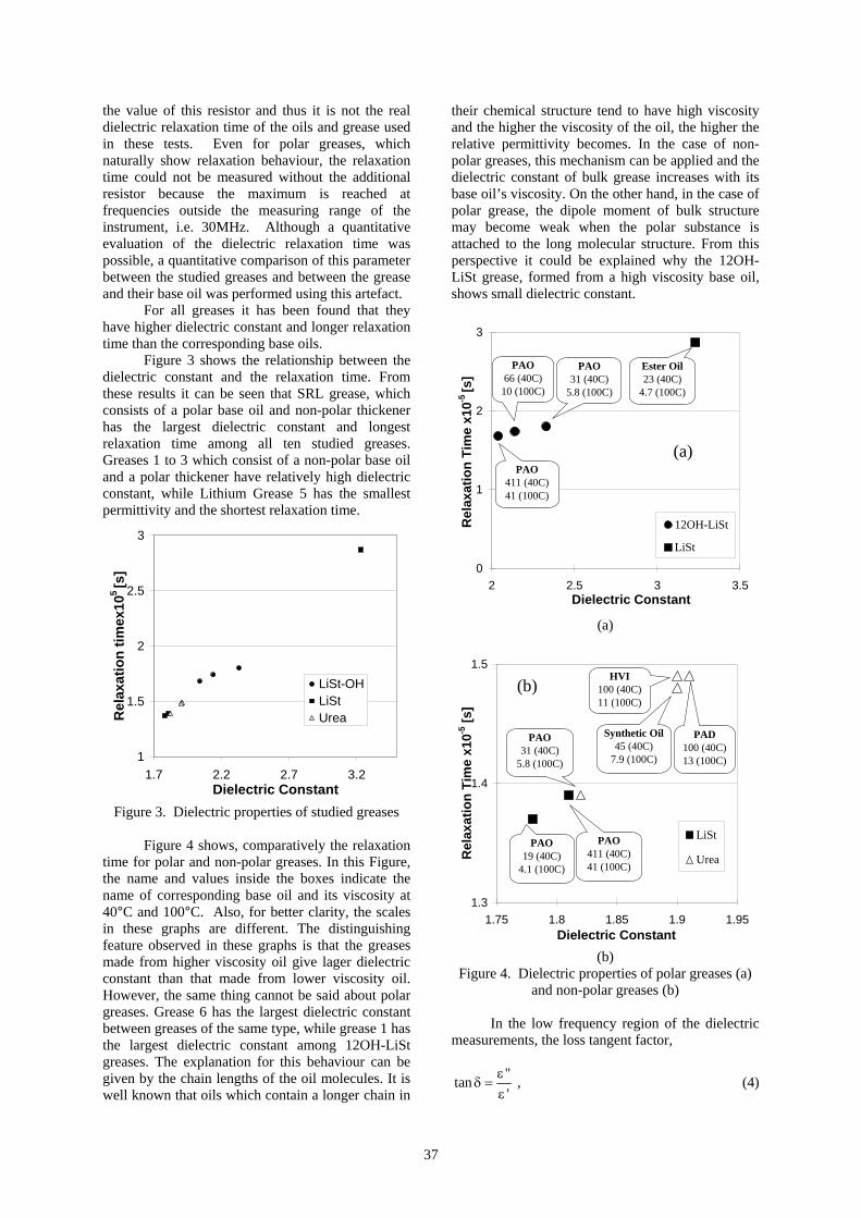
the value of this resistor and thus it is not the real dielectric relaxation time of the oils and grease used in these tests. Even for polar greases, which naturally show relaxation behaviour, the relaxation time could not be measured without the additional resistor because the maximum is reached at frequencies outside the measuring range of the instrument, i.e. 30MHz. Although a quantitative evaluation of the dielectric relaxation time was possible, a quantitative comparison of this parameter between the studied greases and between the grease and their base oil was performed using this artefact.
For all greases it has been found that they have higher dielectric constant and longer relaxation time than the corresponding base oils.
Figure 3 shows the relationship between the dielectric constant and the relaxation time. From these results it can be seen that SRL grease, which consists of a polar base oil and non-polar thickener has the largest dielectric constant and longest relaxation time among all ten studied greases. Greases 1 to 3 which consist of a non-polar base oil and a polar thickener have relatively high dielectric constant, while Lithium Grease 5 has the smallest permittivity and the shortest relaxation time.
1
1.5
2
2.5
3
1.7 2.2 2.7 3.2Dielectric Constant
Rel
axat
ion
tim
ex10
5 [s
]
LiSt-OHLiStUrea
Figure 3. Dielectric properties of studied greases
Figure 4 shows, comparatively the relaxation
time for polar and non-polar greases. In this Figure, the name and values inside the boxes indicate the name of corresponding base oil and its viscosity at 40°C and 100°C. Also, for better clarity, the scales in these graphs are different. The distinguishing feature observed in these graphs is that the greases made from higher viscosity oil give lager dielectric constant than that made from lower viscosity oil. However, the same thing cannot be said about polar greases. Grease 6 has the largest dielectric constant between greases of the same type, while grease 1 has the largest dielectric constant among 12OH-LiSt greases. The explanation for this behaviour can be given by the chain lengths of the oil molecules. It is well known that oils which contain a longer chain in
their chemical structure tend to have high viscosity and the higher the viscosity of the oil, the higher the relative permittivity becomes. In the case of non-polar greases, this mechanism can be applied and the dielectric constant of bulk grease increases with its base oil’s viscosity. On the other hand, in the case of polar grease, the dipole moment of bulk structure may become weak when the polar substance is attached to the long molecular structure. From this perspective it could be explained why the 12OH-LiSt grease, formed from a high viscosity base oil, shows small dielectric constant.
0
1
2
3
2 2.5 3 3Dielectric Constant
Rel
axat
ion
Tim
e x1
0-5 [s
]
.5
12OH-LiSt
LiSt
PAO411 (40C)41 (100C)
PAO66 (40C)
10 (100C)
PAO31 (40C)
5.8 (100C)
Ester Oil23 (40C)
4.7 (100C)
(a)
(a)
1.3
1.4
1.5
1.75 1.8 1.85 1.9 1.95Dielectric Constant
Rel
axat
ion
Tim
e x1
0-5 [
s]
LiSt
Urea
PAO19 (40C)
4.1 (100C)
PAO411 (40C)41 (100C)
PAO31 (40C)
5.8 (100C)
HVI100 (40C)11 (100C)
Synthetic Oil45 (40C)
7.9 (100C)
PAD100 (40C)13 (100C)
(b)
(b) Figure 4. Dielectric properties of polar greases (a)
and non-polar greases (b)
In the low frequency region of the dielectric measurements, the loss tangent factor,
"tan
'
, (4)
37

indicates the electrical conductivity of material [18]. Of all tested greases, only SRL shows good conductivity, as seen in Figure 5, where the tangent loss of SRL grease, grease 1, grease 5 and SB-M, are shown as a function of frequency.
0
1
2
3
1 100 10000 1000000Frequency [Hz]
tan
SRL
SB-M
Grease1
Grease5
Figure 5. Loss tangent factor of four greases
4.2 EHD Traction Measurements
Traction curves of SRL at 10N load are shown in Figure 6.
0
0.01
0.02
0.03
0.04
0.05
0.06
0.07
0 0.2 0.4 0.6 0.8
Slide Roll Ratio
Tra
cti
on
Co
effi
cie
nt
1st test
2nd test
Figure 6. Traction curves for SRL grease
In each test, the measurement of the traction
coefficient was carried out twice. After a first test the rig was left to run for five minutes in pure rolling conditions and after that, the test was run again in order to check whether starvation of the contact occurs, due to the ball pushing the grease to the sides of the track.
Graphs like those seen in Figure 6 can be transformed to show the dependence between the shear stress and shear strain rate. Such dependence
for some of the greases studied in this work is shown in Figure 7.
0
20
40
60
80
1.E+03 1.E+04 1.E+05 1.E+06
Shear strain rate [s-1]
Sh
ea
r s
tre
ss
[M
Pa
]
SRL
Grease5
Grease6
Figure 7. Shear stress function of shear rate
The traction curves obtained were subsequently used in an analysis similar to that done by Evans and Johnson [9], to extract the effective viscosity and the Eyring stress of the tested
lubricants. For large shear strain the hyperbolic sine function can be approximated with an exponential, and for a negligible elastic term, equation (2) becomes:
0
0 00
2ln ln
. (5)
In this relationship, is the shear stress, 0
is the Eyring stress and is the shear rate. In a
logarithmic representation, the slope of the linear region of the shear stress/shear rate dependence, seen in Figure 7 for large values of the shear rate, represents the Eyring stress of the lubricant, as predicted by Equation (5).
In general, the Eyring stress has been found to have similar values of that of the base oils, except four greases, RL2, RLS2, SB-M and SRL, which showed larger Eyring stress than that of the corresponding base oils. As seen in Table 1, RL2, RLS2 and SB-M, have different composition, although for all of them, the thickener is urea based. Their base oil is also different from one another: mineral oil for RL2 and synthetic oils of for RLS2 and SB-M. As shown in Figure 4, these greases have very similar dielectric relaxation times. The SRL grease, on the other hand, is very different from the composition point of view, with a ester base oil and a lithium soap as thickener. The Eyring stress for this grease and its base oil can be seen in Figure 8. As this parameter is not directly measured, but it is calculated as explained above, it is very sensitive
38

to the accuracy of the traction coefficient and film thickness measurements. For this reason, the tests have been repeated and the average values, together with error bars have been shown. It is clear that the Eyring stress of the grease is larger than that of the base oil.
0
5
10
15
0.6 0.8 1 1.2Hertzian pressure [GPa]
Ey
rin
g s
tre
ss
[MP
a]
SRL greaseBase oil
Figure 8. Eyring stress for SRL grease and base oil
1
10
100
1000
0.01 0.10 1.00Entrainment speed [m/s]
Fil
m t
hic
knes
s [n
m]
SRL greaseBase oil
Figure 9. Film thickness measurements of SRL
and its base oil
The shear rate involved in the evaluation of the Eyring stress is determined as the rate between the sliding speed in the contact and the film thickness. A comparison of the central film thickness for the grease and the base oil is shown in Figure 9. For the low speeds region, where the traction coefficient tests have been conducted, the grease has a film thickness about four times larger than that of the base oil. It is not clear, at this point, whether the larger value of the Eyring stress for these greases is a genuine effect, or an experimental artifact, however, the fact that this tendency appeared every time the test was repeated, and that the tests for all greases are done in identical conditions, suggest indeed, among all greases tested
in this study,that their Eyring stress has larger values than their base oil.
0
1
2
3
4
0.6 0.8 1 1.2Hertzian pressure [GPa]
Eff
ec
tiv
e v
isc
os
ity
lo
g10
[Pa
s]
SRL greaseBase oil
Figure 10. Effective viscosity of SRL grease
0
20
40
60
80
1.E+03 1.E+04 1.E+05 1.E+06
Shear strain rate [s-1]
Sh
ea
r s
tre
ss
[M
Pa
]
Grease4RL2RLS2SB-M
Figure 11. Shear stress for urea-type greases
0.E+00
2.E+07
4.E+07
6.E+07
1.E+03 1.E+04 1.E+05 1.E+06
Shear rate [s-1]
Sh
ear
str
ess
[Pa]
Grease1
Grease2
Grease3
Figure 12. Shear stress for 120H-LiSt greases
39

After determining the Eyring stress, from equation (5) the effective, average viscosity of the lubricant inside the contact can be extracted. This was done by fitting equation (5) to the experimental data. The results for SRL grease are shown in Figure 10. As seen, unlike the Eyring stress, the values of the effective viscosity of the grease tend to be below the value of its base oil at high pressure.
From the traction results for all greases, it can be concluded that urea greases tend to show relatively high shear stress. An exception to this rule is SB-M, which shows relatively low shear stress. This grease, which is produced especially as low-noise grease, also has the smallest permittivity among urea greases. Four types of urea greases are compared in Figure 11. Figure 12 shows the shear stress function of the shear rate for polar thickener greases (12OH-LiSt). It can be seen that the shear stress of grease 3 increases slightly and has lower value, at high shear rate, compared with the other greases of the same type. It can be noted that the dielectric results for these greases showed that Grease 1 has the largest permittivity, 2.30, while the dielectric constant of Grease 2 and 3 are 2.15 and 2.06, respectively.
A similar trend was observed for the Li-St greases shown in Figure 7. Grease 6, which has slightly larger dielectric permittivity than Grease 5, also shows larger shear stress. 5. CONCLUSIONS
A dielectric spectroscopy study, coupled with EHD traction measurements were carried out for a number of ten greases with various compositions and properties. The following conclusions have been drawn form this study. (1) From the dielectric measurements, it has been
found that greases always have larger dielectric constant than their base oil and that the base oil has a stronger influence than the thickener on the grease dielectric constant. In greases containing polar components, the dielectric constant of the grease decreases with increasing the viscosity of its base oil. In non-polar greases, on the other hand, the dielectric constant of the grease increases with the viscosity of its base oil.
(2) The dielectric properties, especially in the low frequency range, seem to be related to the film formation in EHD contacts. SRL grease, which has good conductivity, revealed by the dielectric measurements, shows poor film formation ability compared to other greases.
(3) The effective viscosity of grease inside the EHD contact has been calculated from the measured value in traction test and characteristic similar to oil is found in case of grease. The logarithm of viscosity of greases varies linearly with pressure, but the degree of
inclination is moderate compared to base oils. On the other hand, the Eyring stress of greases rapidly increases and it has been found that for three of the studied greases the value of this parameter is greater than that corresponding to the base oil.
(4) From the traction measurements, it can be concluded that, in general, urea thickener greases exhibit large shear stress in their operation. It has also been found that greases with higher dielectric constant show larger shear stress when compared to greases containing the same type of thickener.
ACKNOWLEDGEMENT
Yuichiro Nagata is grateful to Shell and
Kyodo Yushi for supplying their greases and base oils and to professor Joichi Sugimura of Kyushu University, Japan and his colleagues for allocating their greases from NSK. REFERENCES 1. Glovnea, R.P. 2010, “Transient Phenomena in Elastohydrodynamic Lubrication,” Recent development in Wear Prevention, Friction and Lubrications, ed. G. Nikas, Research Signpost Publ., pp. 227-262. 2. Cann, P.M.E., 1999, “Starved Grease Lubrication of Rolling Contacts,” Tribology Transactions, Vol:42, pp. 867-873 3. Eriksson P., Wikstroem V. and Larsson R 2000, “Grease Passing Through an EHD Contact Under Pure Rolling Conditions,” Proc Instn Mech Engrs, 214, pp. 309-316. 4. Couronne, I., Mazuyer, D., Vergne, P., Truong-Dinh, N., Girodin, D. 2003, “Effects of Grease Composition and Structure on Film Thickness in Rolling Contact,” Trib. Trans., vol. 46, 1, pp. 31-36 5. Cann, P.M., Williamson, B.P., Coy, R.C., and Spikes, H.A., 1992, “The Behaviour of Greases in Elastohydrodynamic Contacts,” J. Phys. D: Appl. Phys, 25. 6. Hirst, W., Moore, A.J., 1979, “Elastohydrodynamic Lubrication at High Pressures-Non-Newtonian Behaviour”, Proc. Roy. Soc. Lond., A, 365,pp. 537-565 7. Bair, S., and Winer, WO., 1979, “A Rheological Model for Elastohydrodynamic Contacts Based on Primary Laboratory Data,” J. Lub. Tech., Vol 101, pp.258-265 8. Johnson, K.L., and Tevaarwerk, J.L., 1977, “Shear Behaviour of Elastohydrodynamic Oil Films”, Proc. R. Soc., Lond., Ser.A., 356, pp.215-236
40

41
9. Evans, C.R., and Johnson, K.L., 1986, “The Rheological Properties of Elastohydrodynamic Lubricants,” Proc Instn Mech Engrs, 200, No C5, pp. 303-312. 10. Diaconescu, E.N., 2004, “Solid-Like Properties of Molecular Liquids Subjected to EHD Conditions: Theoretical Investigations,” Proc. ASME/STLE Joint Int. Trib. Conf., 24-27 Oct., Long Beach, USA 11. Furakama, S., and Sumi, T., 1961, “A Dynamic Theory of Piston-Ring Lubrication”, Bull. of JSME, Vol. 4, 16, pp.744-752 12. Hamilton, G.M. and Moore, S.L., 1974, “Measurement of the Oil Film Thickness Between the Piston Rings and Liner of a Small Diesel Engine”, Proc. Inst. Mech. Engrs., Vol 188, pp. 253-261 13. Sherrington, I., and Smith, E.H., 1985 “Experimental Methods for Measuring the Oil-Film Thickness Between the Piston-Rings and Cylinder-Wall of Internal Combustion Engines”, Trib. Int., vol. 18, 6, pp. 315-320
14. Ibrahim, M., and Cameron, A., 1963, “Oil Film Thickness and Mechanisms of Scuffing in Gear Teeth”, Proc. Inst. Mech. Engrs Lubrication and Wear Convention, pp. 228-238 15. Vichard, J.P., 1971, “Transient Effects in the Lubrication of Hertzian Contacts,” J. Mech. Eng. Sci., Vol. 13, pp. 173-189 16. Van Leeuwen, H, H. Meijer, H., Schouten,M., 1987, “Elastohydrodynamic Film Thickness and Temperature Measurements in Dynamically Loaded Concentrated Contacts: Eccentric Cam-Flat Follower”, Fluid film lubrication-Osborne Reynolds Centenary, Elsevier, pp. 611-625 17. Nagata, Y., Furtuna, M.D., Bell, C.A., and Glovnea, R.P., 2008, “Evaluation of Electric Permittivity of Lubricating Oils in EHD Conditions”, Proc. iCAT2008, Dec. 2008, Singapore, p.155-158 18. Aliotta, F., Fontanella, M.E., Galli, G., Lanza, M., Migliardo, P. and Salvato, G., 1983, “Low-Frequency Dielectric Investigations in Polymer-like Lecithin Gels,” J. Phys. Chem., 97, pp.733-736.

ISSN 1220 - 8434 ACTA TRIBOLOGICA Volume 18, (2010), 42-45
Juozas PADGURSKAS1
e-mail: [email protected]
Raimondas KREIVAITIS1
e-mail: [email protected]
Arturas KUPČINSKAS1
e-mail: [email protected]
Raimundas RUKUIŽA1
e-mail: [email protected]
Vytenis JANKAUSKAS1
e-mail: [email protected]
Igoris PROSYČEVAS2
e-mail: [email protected]
1 Department of Mechanical Engineering,
Lithuanian University of Agriculture - Kaunas,
LITHUANIA2 Institute of Physical Electronics
Kaunas University of Technology – Kaunas
LITHUANIA
INFLUENCE OF NANOPARTICLES ONLUBRICITY OF BASE MINERAL OIL
The tribological properties of mineral oil SAE 10 modified withmetallic nanoparticles were investigated. The tribological testswere performed using four-ball test rig. Friction and wear reductionproperties were measured. The positive influence of nanoparticleson lubricity of mineral oil was observed. The best result wasobtained when using the copper nanoparticles for a single metalnanosuspension (0.25 % Cu). Using double metal nanoparticles thebest result show iron – copper nanosuspension (0.125 % Fe + 0.125% Cu). The use of those suspensions was most efficient for purebase mineral oil. The cobalt nanosuspension does not show asignificant increase in lubricity. It was observed thatnanosuspensions stabilize and decrease the friction during the tests.Keywords: nanoparticles, friction wear, lubricity, mineral oil
1. INTRODUCTION
Presently there is an increasing interest in theuse of nanoparticles. A lot of scientists worldwideperform many tests simulating the possibleapplications of nanoparticles. One of the interestingnanoparticles’ applications is to makenanosuspensions in lubricants. It is observed thatmetal or even non-metal nanoparticles have apositive influence on lubrication properties.Nanoparticles suspensions in lubricants cansignificantly reduce friction and wear of frictionsurfaces [1-5].
Such factors as the material, size, shape andmechanical properties of nanoparticles, theirconcentration in the suspension have importantinfluence on tribological properties of friction pairs[1,2].
Usually the lubricants are modified by thenanoparticles of metal or metal oxide (Cu, CuO,TiO2, ZrO2, ZnO and so on) and some non-metalmaterials (SiO2, diamond, inorganic fullerene,graphite) [1-7]. It is highly evident that only a smallamount of nanoparticles is required to obtain thepositive tribological effect: 0.01 % graphite [6],<1 % diamond [1], 1 % TiO2 [1], 5 % IF-WS2 [4],0.5...2 % CuO, ZnO, ZrO2 [3], 0.2 % SiO2 [7].
Usually, the main research purpose is to estimateoptimal concentration [3,7].
In most cases the commonly manufacturednanoparticles are simply added to the lubricants [3,4,6,7]. However there is increasing interest onsynthesis nanosuspensions by the sintering ofnanoparticles directly in the lubricants [8]. The aimof our study is to estimate the tribological propertiesof some nanosuspensions directly sintered in thebase mineral oil.
2. EXPERIMENT
The synthesis of Fe, Cu, Co and Fe+Cu,Fe+Co, Co+Cu nano-particles is performed by theCEWLS method when the converse emulsion ofwater in lubricant synthesis is used. For that reasonis prepared 100 ml mineral oil SAE10 emulsion with0.2 ml H2O which includes dissolved sulphates ofcertain metals, such as FeSO4, CuSO4, CoSO4 and0.5 g cetyltrimenthylammonium bromide (CTAB).This mixture is poured into 100 ml of mineral oilSAE10 with 10 ml hydrazine emulsion. All volumewas mixed intensively during 5 minutes. Thismixture with formed according nano-particles wasused for tribological investigations. Theconcentrations of nanoparticles in suspensions using

43
single metal were 0.25 %, using double metalnanoparticles – 0.125 % of each metal in compound.
Four-ball type tribotester was used for wearand friction tests. The balls of 12.7 mm diameterwere made of 100Cr6 bearing steel. The testingprocedure was adapted from the standardDIN 51 350 [9].
The test oil sample of 22 cm3 was poured intothe sample chamber, fully submerging the stationaryballs. Under the applied load of 150 N, and rotationspeed of 1420 rpm, the machine was run for 1 hour.Prior to each experiment, all the appropriate parts ofthe machine, i.e. bottom and upper ball holders, oilvessel and the test balls were washed in an ultrasonicbath with hydrocarbon solvents, and then dried.
The diameters of the circular wear tracks(wear scars) on three stationary balls were measuredwith an optical microscope. For each run the scarmeasurements were reported as an average of theWear Scar Diameter (WSD) of the three balls inmillimetres. Friction between the balls is representedby torque.
3. RESULTS AND DISCUSSIONS
The results of performed tests are presentedin Figure 1. It shows that all used suspensions ofnanoparticles decrease the wear and frictioncomparing to pure mineral base oil SAE 10.However the positive influence was not equal for allsuspensions.
0,0
0,2
0,4
0,6
0,8
SAE 10 SAE 10 +Fe
SAE 10 +Cu
SAE 10 +Co
SAE 10 +FeCu
SAE 10 +FeCo
SAE 10 +CoCu
Test Oil (Composition)
WSD
, mm
0
10
20
30
40
50
60
70
Ave
rage
torq
ue, m
Nm
.
Wear Average torque
Figure 1. Wear and friction behaviour of base oil and metal nanosuspensions
The best result was obtained using coppernanoparticles when using single metalnanosuspension and the worst one when using cobaltnanoparticles.
Lubrication with copper nanosuspensionreduces the wear 1.87 times and the friction – 1.54times comparing to base oil. Wear reduction wasless important when using iron nanosuspensions incomparison to copper. However the frictionreduction was virtually the same for both thosenanosuspensions. The wear and friction reduction ofcobalt nanosuspension was almost negligible.
It is likely that wear and friction reductionproperties of copper nanosuspension are related toits mechanical properties. The soft and ductilematerial can easily get between contacting surfacesand cover them making good protection against thewear.
Estimation of wear and friction behaviour of
double metal nanoparticles displays that the bestresult of all tested nanosuspensions shows iron –copper nanosuspension. Lubrication with iron –copper nanosuspension reduces the wear almost twotimes, and the friction – 1.76 times. Such a greatincrease in lubricity can be due to combination oftwo metals with different mechanical properties andof course different interaction mechanisms.
Despite that cobalt does not reduce the wearsignificantly in single metal nanosuspension tests, incombination with iron and copper it has much betterlubricity. The suspension of cobalt–coppernanoparticles reduces the wear and frictionrespectively 1.78 and 1.75 times comparing to baseoil.
Friction torque variation graphs during theentire test (Figures 2 and 3) were used for frictionanalysis. Figure 2 presents the friction torque whenlubricating with single metal nanosuspension.

44
20
40
60
80
100
0 1000 2000 3000 4000Test duration, s
Tor
que,
mN
m
,
SAE 10
SAE 10 + Cu
SAE 10 + Co
SAE 10 + Fe
Figure 2. Friction torque variation during the test using the lubrication withpure base oil and single metal nanosuspensions
20
40
60
80
100
0 1000 2000 3000 4000Test duration, s
Tor
que,
mN
m ,
SAE 10
SAE 10 + FeCo
SAE 10 + CoCu
SAE 10 + FeCu
Figure 3. Friction torque variation during the test using the lubrication withpure base mineral oil and double metal nanosuspensions
Usually friction torque increases during thetests when using the pure base oil. Regardless somefluctuations it was also the case in ourinvestigations. Using the nanosuspensions the
fluctuations almost disappear. Moreover, thefriction value has decreasing trend during the testwhen using the nanosuspensions of single copperand iron.

45
Slightly different results were obtained whenusing double metal nanosuspensions (Figure 3).
Friction torque values are stabile for thosesuspensions, but we have no friction decreasetendency for FeCo nanosuspension. It was almost nodifference between the friction behaviour of CoCuand FeCu nanosuspensions. The reason for thatcould be much more important influence of copperon tribological properties of double metalnanosuspensions.
4. CONCLUSIONS
Metallic nanoparticles’ suspensions obtainedby direct sintering in the lubricant are efficient forwear and frictions reduction. Moreover all usednanosuspensions help to increase friction stability.
Copper and iron – copper nanoparticles’suspensions presented the best lubricationproperties, Co nanosuspensions – the worst.
ACKNOWLEDGEMENT
This research was funded by Lithuanian StateScience and Studies Foundation grant B-34/2008"NanoTribo-Suspensions".
REFERENCES
1. Wu Y. Y., Tsui W. C., Liu T. C., 2007,“Experimental Analysis of Tribological Properties ofLubricating Oils with Nanoparticle Additives,”Wear, 262, p. 819 – 825.
2. Hernández Battez A., González R.,Felgueroso D., and other, 2007, “Wear PreventionBehavior of Nanoparticles Suspension underExtreme Pressure Condition,” Wear, 263, p. 1568 –1574.3. Hernández Battez A., González R.,Felgueroso D., and other, 2008, “CuO, ZrO2 andZnO Nanoparticles as Antiwear Additive in OilLubricants,” Wear, 265, p. 422 – 428.4. Rapoport L., Leshchinsky V., Lapsker I., andother, 2003, “Tribological Properties of WS2
Nanoparticles under Mixed Lubrication,” Wear, 255,p. 785 – 793.5. Rapoport L., Nepomnyashchy O., Lapsker I.,and other, 2005, “Behavior of Fullerene – like WS2
Nanoparticles under Severe Contact Conditions,”Wear, 295, p. 703 – 707.6. Huang H. D., Tu J. P., Gan L. P., Li C. Z.,2006, “An Investigation on Tribological Propertiesof Graphite Nanosheets as Oil Additives,” Wear,261, p. 140 – 144.7. Peng D. X., Kang Y., Hwang R. M., and other,2009, “Tribological Properties of Diamond and SiO2
Nanoparticles Added in Paraffin,” TribologyInternational, 42, p. 911 – 917.8. Padgurskas J., Rukuiža R., Kreivaitis R., andother, 2009, “Tribological Properties of Mineral OilsModified with Metallic Nano-Particles,”Proceedings of 5th International ScientificConference „BALTTRIB 2009“, LithuanianUniversity of Agriculture, Kaunas, p. 69-76.9. DIN 51350-3, Testing of lubricants - Testing inthe four-ball tester- Part 3: Determination of wearingcharacteristics of liquid lubricants, 1977 (InGermany).

ISSN 1220 - 8434 ACTA TRIBOLOGICA Volume 18, (2010), 46-51
Alexandru V. RADULESCU1
e-mail: [email protected]
Irina RADULESCU2
e-mail: [email protected]
1 Department of Machine Elements and Tribology,
University POLITEHNICA Bucharest,
ROMANIA2 Mechanical Engineering and Research Institute
S. C. ICTCM S.A. Bucharest,
ROMANIA
INFLUENCE OF THE RHEOMETER GEOMETRYON THE RHEOLOGICAL PROPERTIES OFINDUSTRIAL LUBRICANTS
The rheological properties of two transmission lubricants (75W90and 75W140), in fresh and used state, were investigated using shearviscosity rheological measurements. It was found that the lubricantsdo not exhibit a yield stress and that, above a critical shear rate, theyexhibit shear-thinning behavior, well described by the Cross model.The rheological measurements were performed on a Brookfieldviscometer CAP2000+ equipped with four cone-and-plategeometry, for a range of temperature between 20 … 70°C, using theviscometer Peltier system. The experiments have shown that onlytwo geometries are appropriate for testing the transmissionlubricants. Another important conclusion refers to the influence ofthe wear degree of the lubricant on the rheological parameter of themodel.Keywords: viscosity, lubricants, shear-thinning, wear
1. INTRODUCTION
Rheological modeling of lubricants hasalways been a subject of great importance whenworking with oil from different fields of interest.The need for predicting the rheological behavior ofthe lubricants when experiencing conditions outsidethe available measuring range for the equipmentdesigned in accordance with API specifications [1,2]has always been present.
Transmission lubricants behave in a non-Newtonian way. They are shear-rate dependent andnormally termed as shear-thinning lubricants.Rheological measurements are normally performedin the laboratory within a given range of shear rates.Based on these measured values the models shouldbe able to predict the shear-dependent behavior ofthe lubricants outside the measured interval of shearrates.
The rheological properties of twotransmission lubricants (75W90 and 75W140), infresh and used state, were investigated using shearviscosity rheological measurements. It was foundthat the lubricants do not exhibit a yield stress andthat, above a critical shear rate, they exhibit shear-thinning behaviour, well described by the Crossmodel. Supplementary tests have been made,regarding the thermal behaviour of the lubricants.Three thermal models have been assumed, in orderto determine the variation of the viscosity with thetemperature, for lubricants in fresh and used state.
2. THEORY
The rheological model based on the Crossequation is one of the most popular in use today. Itcan be found on virtually every research rheometersoftware packages and it can be used to extract somemeaningful numbers from the “full” viscosity versusshear rate profile (Fig. 1).
The mathematical expression of the the Crossmodel is described by the Eq. (1), [3]:
0
m1
, (1)
where is the shear rate and η is the viscosity at any
given shear rate .
The other parameters involved in eq. (1) are: η0 is the zero shear viscosity and represents
the magnitude of the viscosity at the lowerNewtonian plateau. It is a critical material propertyand can prove valuable in making assessments ofsuspension and emulsion stability, estimating ofcomparative polymer molecular weight and trackingchanges due to process or formulation variables etc.
η∞ is the infinite shear viscosity. Thissignifies how the product is likely to behave in veryhigh shear processing situations such as blade, knifeand roller coating.
λ is known as the Cross time constant and hasdimensions of time. The reciprocal, 1/ λ, gives a
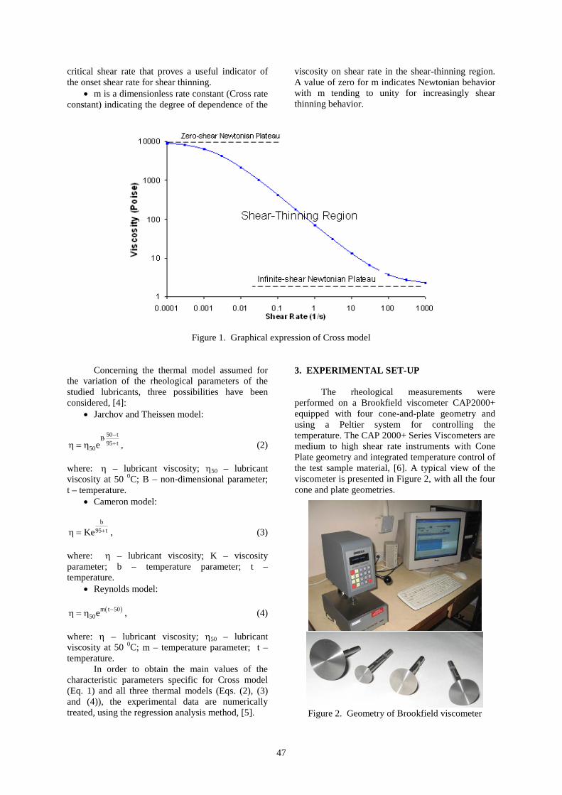
47
critical shear rate that proves a useful indicator ofthe onset shear rate for shear thinning.
m is a dimensionless rate constant (Cross rateconstant) indicating the degree of dependence of the
viscosity on shear rate in the shear-thinning region.A value of zero for m indicates Newtonian behaviorwith m tending to unity for increasingly shearthinning behavior.
Figure 1. Graphical expression of Cross model
Concerning the thermal model assumed forthe variation of the rheological parameters of thestudied lubricants, three possibilities have beenconsidered, [4]:
Jarchov and Theissen model:
50 tB
95 t50e
, (2)
where: – lubricant viscosity; 50 – lubricantviscosity at 50 0C; B – non-dimensional parameter;t – temperature.
Cameron model:
b
95 tKe , (3)
where: – lubricant viscosity; K – viscosityparameter; b – temperature parameter; t –temperature.
Reynolds model:
m t 5050e , (4)
where: – lubricant viscosity; 50 – lubricantviscosity at 50 0C; m – temperature parameter; t –temperature.
In order to obtain the main values of thecharacteristic parameters specific for Cross model(Eq. 1) and all three thermal models (Eqs. (2), (3)and (4)), the experimental data are numericallytreated, using the regression analysis method, [5].
3. EXPERIMENTAL SET-UP
The rheological measurements wereperformed on a Brookfield viscometer CAP2000+equipped with four cone-and-plate geometry andusing a Peltier system for controlling thetemperature. The CAP 2000+ Series Viscometers aremedium to high shear rate instruments with ConePlate geometry and integrated temperature control ofthe test sample material, [6]. A typical view of theviscometer is presented in Figure 2, with all the fourcone and plate geometries.
Figure 2. Geometry of Brookfield viscometer
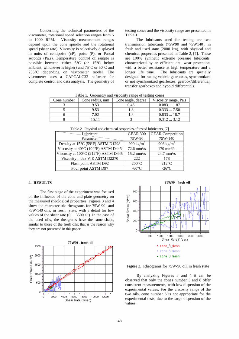
48
Concerning the technical parameters of theviscometer, rotational speed selection ranges from 5to 1000 RPM. Viscosity measurement rangesdepend upon the cone spindle and the rotationalspeed (shear rate). Viscosity is selectively displayedin units of centipoise (cP), poise (P), or Pascalseconds (Pa.s). Temperature control of sample ispossible between either 5°C (or 15°C belowambient, whichever is higher) and 75°C or 50°C and235°C depending on viscometer model. Theviscometer uses a CAPCALC32 software forcomplete control and data analysis. The geometry of
testing cones and the viscosity range are presented inTable 1.
The lubricants used for testing are twotransmission lubricants (75W90 and 75W140), infresh and used state (2000 km), with physical andchemical properties presented in Table 2, [7]. Theseare 100% synthetic extreme pressure lubricants,characterized by an efficient anti wear protection,with a better resistance at high temperature and alonger life time. The lubricants are speciallydesigned for racing vehicle gearboxes, synchronizedor not synchronized gearboxes, gearbox/differential,transfer gearboxes and hypoïd differentials.
Table 1. Geometry and viscosity range of testing conesCone number Cone radius, mm Cone angle, degree Viscosity range, Pa.s
3 9.53 0.45 0.083 ... 1.875 9.53 1.8 0.333 ... 7.506 7.02 1.8 0.833 ... 18.78 15.11 3 0.312 ... 3.12
Table 2. Physical and chemical properties of tested lubricants, [7]LubricantParameter
GEAR 30075W-90
GEAR Competition75W-140
Density at 15°C (59°F) ASTM D1298 900 kg/m3 906 kg/m3
Viscosity at 40°C (104°F) ASTM D445 72.6 mm²/s 170 mm²/sViscosity at 100°C (212°F) ASTM D445 15.2 mm²/s 24.7 mm²/s
Viscosity index VIE ASTM D2270 222 178Flash point ASTM D92 200°C 212°CPour point ASTM D97 -60°C -36°C
4. RESULTS
The first stage of the experiment was focusedon the influence of the cone and plate geometry onthe measured rheological properties. Figures 3 and 4show the characteristic rheograms for 75W-90 and75W-140 oils, in fresh state, with a detail for lowvalues of the shear rate (0 ... 3500 s-1). In the case ofthe used oils, the rheograms have the same shape,similar to those of the fresh oils; that is the reason whythey are not presented in this paper.
Figure 3. Rheograms for 75W-90 oil, in fresh state
By analyzing Figures 3 and 4 it can beobserved that only the cones number 3 and 8 offerconsistent measurements, with low dispersion of theexperimental values. For the viscosity range of thetwo oils, cone number 5 is not appropriate for theexperimental tests, due to the large dispersion of thevalues.

49
Figure 4. Rheograms for 75W-140 oil, in fresh state
The cone number 8 is characterized by a lowshear rate range (0 …. 2000 s-1), while the conenumber 3 has a larger shear rate range, between 0 s-1
and 13300 s-1. The tests with this geometry offerresults which can characterize the behavior of thelubricant for a vaster interest domain.
The experimental results obtained with conesnumber 3 and 8 have been treated with theregression analysis method, according to the Crossmodel (Eq. 1), in order to obtain the variation of theviscosity with the shear rate. The parameters of theCross model are presented in Table 3, and thecomparison between the experimental resultsobtained with cone number 3 and the theoreticalmodel is shown in Figures 5 and 6.
It can be observed significant differencesbetween cone 3 and 8, caused be the extended fieldof the shear rate values. Another importantconclusion refers to the influence of the wear degreeof the lubricant on the rheological parameter of theCross model. For the 75W90 oil, there are almostno differences between fresh and used lubricant(Fig. 5) while the oil 75W140 presents importantchanges in used state comparative to fresh state (Fig.6). The same observation can be made for the twooils regarding the variation of the viscosity withtemperature.
The experimental results are presented inFigures 7 and 8 and Table 4 shows the values of therheological parameters of the studied lubricants.
Table 3. Parameters of the Cross model for the transmission lubricantsCross model
Type of oil Wear degree Cone number , Pa·s 0 , Pa·s , s m
3 0.153 0.229 7.595·10-4 0.065fresh
8 0.068 0.275 6.028·10-3 0.1473 0.118 0.307 3.057·10-3 0.175
75W90used
8 0.061 0.263 2.045·10-3 0.1113 0.257 0.628 1.725·10-3 0.104
fresh8 0.213 0.601 1.212·10-3 0.0373 0.220 0.574 1.753·10-3 0.095
75W140used
8 0.151 0.529 7.362·10-4 0.149
75W90 - comparison between fresh and used oil
0.15
0.17
0.19
0.21
0.23
0 2000 4000 6000 8000 10000 12000 14000
Shear rate, 1/s
Visc
osity
, Pa.
s
fresh - exp. used - exp. fresh - th. used - th.
Figure 5. Comparison between the experimental results and the theoretical model for 75W-90 oil (cone no. 3)

50
75W140 - comparison between fresh and used oil
0.350.37
0.390.41
0.430.45
0 2000 4000 6000 8000 10000 12000 14000
Shear rate, 1/s
Visc
osity
, Pa.
s
fresh - exp. used - exp. fresh - th. used - th.
Figure 6. Comparison between the experimental results and the theoretical model for 75W-140 oil (cone no. 3)
Table 4. Variation of the rheological parameters of lubricants with temperatureJarchov and Theissen
modelCameron model Reynolds model
Parameter
Lubricant50,Pas
BCorr.coeff. K, Pas b, 0C
Corr.coeff.
50,Pas
m, 0C-1 Corr.coeff.
Fresh 0 .0446 5.419 0.9981 1.97910-4 785.75 0.9981 0 . 0 4 3 5 -0.0473 0.999675W90
Used 0 .0446 5.517 0.9976 1.77610-4 799.97 0.9976 0 . 0 4 3 2 -0.0478 0.9995Fresh 0 .1043 5.232 0.9986 5.57210-4 758.58 0.9986 0 . 1 0 2 1 -0.0454 0.9995
75W140Used 0 .0919 5.520 0.9994 3.67810-4 800.46 0.9994 0 . 0 8 9 9 -0.0477 0.9989
Figure 7. Variation of the viscosity with temperature for 75W90 oil
Figure 8. Variation of the viscosity with temperature for 75W140 oil

51
5. CONCLUSIONS
The experimental results were found to be welldescribed by the Cross model, except for theviscometer geometries number 5 and 6. It can beobserved also significant differences between cone 3and 8, caused be the extended field of the shear ratevalues. Another important conclusion refers to theinfluence of the wear degree of the lubricant on therheological parameter of the model, including thevariation with temperature.
REFERENCES
1. Qemada, D., 1998, “Rheological Modeling ofComplex Fluids I. The Concept of Effective Volume
Fraction Revisited,” Eur. Phys. J., Appl. Phys. 1, pp.119–127.2. *** , 1990, Specification for Materials andTesting for Well Cements, 5th edn., API Spec., vol.10, American Petroleum Institute, Dallas, TX, USA3. Cross, M.M., 1965, “Rheology of Non-Newtonian Fluids: A New Flow Equation forPseudoplastic Systems,” Journal of Colloid Science,Vol. 20, No. 5, p. 417-437.4. Balan, C. (compiled author), 2000, TheRheology of Lubricating Greases, ELGI,Amsterdam, 160 p.5. Crocker, D.C., 1983, “How to Use RegressionAnalysis in Quality Control,” American Society forQuality Control, Vol. IX, 243 p.6. *** Oil catalog MOTUL France,http://www.motul.fr/fichestechniques/Transmission.

ISSN 1220 - 8434 ACTA TRIBOLOGICA Volume 18, (2010), 52-57
Vlad – Flaviu ZEGREANemail: [email protected]
Emanuel DIACONESCU
Department of Applied Mechanics,
University “Stefan cel Mare” of Suceava,
ROMANIA
MEASUREMENT OF LUBRICANT OILMICROVISCOSITY BASED ON RESONANTFREQUENCY SHIFT OF AFM CANTILEVER
Experimental investigations on microviscosity of T90 lubricant oilwere conducted using an atomic force microscope. The resonantfrequency of the cantilever beams was measured in air, in purewater and in sample oil. Based on the resonant frequency shift theviscosity of the lubricant was calculated using the formula deductedby Papi [1] for uncalibrated cantilevers. The results obtained are ingood agreement with those of Ionescu [2], measured with aRheotest2 rheometer, for the same lubricant.Keywords: microviscosity, atomic force microscopy, resonantfrequency shift
1. INTRODUCTION
Since its invention by Binning at al. in 1986[3], the atomic force microscope (AFM) gainedever-increasing importance in nanotechnology andbiotechnology. The AFM is now widely used toobtain high-resolution surface topography images, tomeasure intermolecular forces or to characterize themechanical properties of polymers. The capabilityof the AFM to take measurements with thecantilever and sample submerged in a liquid enhancethe image resolution due to reduced capillary forces.
There are two operating modes for atomicforce microscopy:
Contact mode, when the cantilever tip is inpermanent contact with the sample. Usingthis mode, the friction force between the tipand the sample can be measured. Thisimaging mode dramatically reduces thelifetime of the tip.
Tapping mode, when the tip is kept above thesample by the feedback loop. In thisoperating mode, the cantilever is driven atresonant frequency, near the surface of theprobe by acoustic, magnetic or Brownianmethods. The amplitude and phase of tiposcillation are then used to extractinformation about the sample topography.The frequency of cantilever vibration
immersed in a fluid strongly depends on the fluidrheological properties. The drag forces acting oncantilever are directly related to kinematic viscosityand fluid density. Thus the viscosity of the fluid canbe determined from the resonant frequency of thecantilever.
2. THEORETICAL CONSIDERATIONS
To our best knowledge, existing research didnot provide a simple and general relationshipbetween fluid viscosity and cantilever resonantfrequency. The attempt to find a relationship todescribe the dependence of fluid viscosity oncantilever resonant frequency can be classified ontwo broadly approaches.
Viscous model proposed by Sader [4] andexperimentally validated by Chon at al. [5] accountsall the geometrical parameters of the cantilever.Sader assumed that the beam cross section isuniform over the entire length, the length of thebeam greatly exceeds its width, b, the beam is ananisotropic linearly elastic solid and internalfrictions effects are negligible, the amplitude ofvibration is far smaller than any length scale of thebeam geometry. The expression that correlates the
normalized Reynolds number, Re , on frequencyresponse of the cantilever is:
2vac,1bRe4
, (1)
where is the fluid density, vac,1 is the
fundamental radial resonant frequency of the beamin vacuum and is the fluid viscosity.
Classical model that draws a heuristicanalogy with the dynamic motion of a sphere troughviscous fluid was approached by Chen [6], Oden [7],and Ahmed [8].
The calculation of viscosity using thisapproaches rely on accurate values of cantileverthickness, coating thickness, mass, density and

53
elastic modulus. The calibration procedure of thecantilever is time consuming, presents the risk ofdamaging the cantilever, or has to be reinitiatedwhen viscosity changes.
To overcome these difficulties, Papi [9]proposed a method for determining the absolutevalue of fluid viscosity by accounting for thecantilever resonant frequency measured in air orvacuum, in the sample solution and in a liquid ofknown viscosity as a standard.
Based on the classical model, Papi [1] findsthe following mathematical expression to correlatethe sample viscosity, s , to resonant frequencies:
2
2 2
s ss H O
H O H O
Y
Y
, (2)
where s ,2H O are the resonant frequencies of the
cantilever submerged in sample solution,respectively in pure water (used as a standardliquid), and sY ,
2H OY are two dimensionless
parameters yielding from:
2
2
2
22 20 s,H O
s,H O 2s,H O
Y
. (3)
The parameter is a combination of
cantilever beam geometry and structure parametersand its value can be set as unity for the greatmajority of common commercial cantilevers.
3. EXPERIMENTAL PROCEDURE
To measure the resonant frequency of thecantilever, a Nanonics Imaging Multiview 1000AFM, depicted in Figure 1, was used. Thecantilever is acoustically driven in a range offrequencies set by user and the resonant frequency isdetected by the optical device of the AFM.
The Nanonics NWS software allows tracingthe sweep curve, setting the oscillation amplitude ofthe cantilever and setting the input gains for thesignal.
Figure 1. Nanonics Imaging Multiview 1000 AFM and Academia optical microscope
In order to submerge the cantilever, a ParkScientific Instruments Universal SPM liquid cellwas modified to fit the Nanonics sample and probemount, Figure 2. A small liquid tank was attachedto a sample mount, Figure 2(a). A transparent thinflat glass window with a plastic collar was fitted tothe probe mount, Figure 2(b). The probe mount ismagnetically connected to the AFM head.
A spring clasp for standard silicon – nitrideprobes, Figure 2(b), was firmly attached under theglass window. The radius of the glass window issmaller than the interior radius of the tank and itsubmerges partially in the liquid along with thecantilever chip, Figure 2(a). Two mirrors are used todirect the laser beam from the source on the surfaceof the cantilever and the reflected beam to the photo-sensitive detector, Figure 2(b).

54
(a)
(b)Figure 2. (a) Modified PSI liquid cell mounted on the Nanonics AFM head; (b) Detail on modified probe mount
Figure 3. Rectangular PSI cantilever
Probe mount
Spring clasp
Liquid tank
Sample mount
NanonicsAFM head
Spring clasp
Plasticcollar
Glasswindow
Probemount
Cantilever chip

55
A rectangular shaped Park ScientificInstruments MicroMash cantilever was used in thisexperiment, Figure 3. The laser spot is reflected bythe first mirror on the far edge of the rectangularcantilever for a maximum deflection angle. Therectangular cantilever was chosen to reduce thedamping effect on the oscillation when the cantileveris immersed in the viscous lubricant oil.
This image was captured with a CCD cameramounted on an Academia optical microscope, Figure1.
4. EXPERIMENTAL RESULTS
The first frequency sweep curve was traced inair with the liquid tank empty, Figure 4. Thefrequency range was set from 0 to 20 kHz and themeasurements were made in 500 points across thisrange. The values displayed are averaged values ofthree consecutive measurements in each point. Themaximum amplitude corresponds to the resonantfrequency of the cantilever. The gain set for thismeasurement was 0.08. The maximum amplitude of0.86751 V was reached at a frequency of 11.9038kHz.
The liquid tank was then filled with purewater at 20oC, measured by a thermocouple and a
new frequency sweep curve, Figure 5, was tracedafter the laser was realigned. The realignment isnecessary because refractive index of water modifythe reflection angle of the laser beam. Results wereaveraged on ten consecutive measurements for aprecise result. The frequency range was limited to 0– 8 kHz because the resonant frequency is lower in aliquid than in air. The input gain was increased to0.1 and the maximum amplitude of 1.2133 V at6.6262 kHz resonant frequency.
After the tank was drained and dried, T90lubricant oil at 30oC was poured into it and the laserwas realigned. Because the lubricant is lesstransparent to laser than pure water the input gainwas increased to 3.2. The frequency range wasgradually reduced down to 0 – 3 kHz. Maximumamplitude of 3.08057 V was reached at 1.9697 kHzresonant frequency, Figure 6.
The resonant frequencies experimentallyobtained in air, pure water and T90 lubricant oil areused in Papi’s formula (2). Considering the waterviscosity
2H O 0.00113 Pa s , the absolute value
of lubricant kinematic viscosity is T90 0.265804 Pa s . The result is in good agreement with thevalues obtained by Ionescu, [2], on a Rheotest 2rheometer on T90 lubricant oil in a range oftemperatures from 17oC to 100oC.
Figure 4. Frequency sweep curve of cantilever in air

56
Figure 5. Frequency sweep curve of cantilever in pure water
Figure 6. Frequency sweep curve of cantilever in T90 lubricant oil
Table 1. Experimental viscosity of T90 measured with Rheotest 2, [2]Temperature
(oC)Viscosity
(Pa.s)17 0.480785330 0.272684240 0.150693950 0.089698760 0.057407270 0.035879580 0.021527790 0.0143518
100 0.0107638

57
5. CONCLUSIONS
A Nanonics MultiView 1000 AFM fromLaboratory of Micro and Nanotribology at theUniversity of Suceava was used to determine theresonant frequency of a rectangular PSI MicroMashcantilever. To enable cantilever submersion, a ParkScientific Instruments Universal SPM liquid cellwas modified to fit the Nanonics head.
The microviscosity of T90 transmissionlubricant oil was measured at 30 oC, by means ofresonant frequency shift of an AFM cantilever inthree different mediums: air, pure water and oil.
The fundamental resonant frequencymeasured in air is 11.9038 kHz, decrease to 6.6262kHz when measured in pure water and reached1.9697 kHz resonant frequency if submerged insample lubricant oil.
The obtained results were applied in Papi’sformula for viscosity determination by means ofuncalibrated atomic force microscopy cantilevers.The absolute value of viscosity, T90 0.265804 Pa s , is in good agreement with the results obtainedby Ionescu with a Rheotest 2 rheometer.
REFERENCES
1. Papi, M., Arcovito, G., De Spirito, M.,Vassalli, M., Tiribilli, B., 2006, “Fluid ViscosityDetermination by Means of Uncalibrated AtomicForce Microscopy Cantilevers,” Applied PhysicsLetters, 88, 194102.
2. Ionescu M., 2004, “A System for ViscosityMeasurement in Variable Conditions of Temperatureand Pressure,” MOCM 10, Vol.1, 205 – 208.3. Binning G., Quate C.F., Gerber Ch., 1986,“Atomic Force Microscope,” Phys. Rev. Lett. 56,930 – 933.4. Sader, J.E., 1998, “Frequency Response ofCantilever Beams Immersed in Viscous Fluids withApplications to the Atomic Force Microscope,”Journal of Applied Physics, 84, 64 – 76.5. Chon, J.W.M., Mulvaney, P., Sader, J.E.,2000, “Experimental Validation of TheoreticalModels for the Frequency Response of AtomicForce Microscope Cantilever Beams Immersed inFluids,” Journal of Applied Physics, 87, 3978 –3988.6. Chen, G.Y., Warmack, R.J., Thundat, T.,Allison, D.P., Huang, A., 1994, “ResonanceResponse of Scanning Force MicroscopyCantilevers,” Rev. Sci. Instrum., 65(8), 2532 – 2537.7. Oden, P.I., Chen, G.Y., Steele, R.A.,Warmack, R.J., Thundat, T., 1996, “Viscous DragMeasurements Utilizing MicrofabricatedCantilevers,” Applied Physics Letters, 68, 3814 –3816.8. Ahmed, N., Nino, D.F., Moy, V.T., 2001,“Measurement of Solution Viscosity by AtomicForce Microscopy,” Rev. Sci. Instrum., 72(6), 2731 –2734.9. Papi, M., Maulucci, G., Arcovito, G., Paoletti,P., Vassalli, M., De Spirito, M., 2008, “Detectionof Microviscosity by Using Uncalibrated AtomicForce Microscopy Cantilevers,” Applied PhysicsLetters, 93, 124102.

ISSN 1220 - 8434 ACTA TRIBOLOGICA Volume 18, (2010), 58-64
M.C. CORNECI1,2
e-mail: [email protected]
A.-M. TRUNFIO-SFARGHIU1
F. DEKKICHE3,4
Y. BERTHIER1
M.-H. MEURISSE1
J.-P. RIEU3
1 Laboratoire de Mécanique des Contacts et des
Structures, INSA-Lyon, CNRS UMR5259,
F69621 Villeurbanne Cedex, FRANCE2 Université Technique “Gh. Asachi”, Faculté de
Mécanique, 700050, Iasi, ROUMANIE3 Laboratoire de Physique de la Matière
Condensée et Nanostructures, Université Claude
Bernard Lyon 1, CNRS UMR5586, F69622
Villeurbanne Cedex, FRANCE4 Département de Chimie, Faculté de Sciences
exactes. Université Mentouri Constantine (25000),
ALGERIE
INFLUENCE OF LUBRICANTPHYSICOCHEMICAL PROPERTIES ON THETRIBOLOGICAL OPERATION OF FLUID PHASEPHOSPHOLIPID BIOMIMETIC SURFACES
Phospholipid bilayers appear to play a key role in joint lubricationin controlling and reducing frictional forces between biologicalsurfaces. We have investigated the mechanical and tribologicalproperties of Dioleoyl phosphatidylcholine (DOPC) bilayersprepared by the micelle and vesicle method in different solutions(ultrapure water and Tris buffer pH 7.2 with or without 150 mMNaCl). Friction forces are measured using a homemadebiotribometer. Mechanical resistance to indentation is measured byAFM and lipid bilayer degradation is controlled in-situ duringfriction testing using fluorescence microscopy. This study confirmsthat mechanical stability under shear or normal load is essential toobtain low and constant friction coefficients. The major result isthat the Tris buffer pH 7.2 improves mechanical and tribologicalstability of the studied bilayers. In ultrapure water, bilayers obtainedby the micelle method are not resistant and spontaneously adsorb tothe other contacting surface. Bilayers prepared by the vesiclemethod show slightly better lubricant properties than those preparedby the micelle method. Additional salt (150 mM NaCl) has existingbut secondary effects on the mechanical and tribological propertiesof the bilayers.Keywords: supported phospholipid bilayers, biolubrication, atomicforce microscopy, friction coeficient, nanomechanics
1. INTRODUCTION
Phospholipids, together with proteins, are themajor components of biological membranes andplay vital roles in many biological processes. Inparticular, phospholipid layers are found in thesynovial fluid and appear to play a key role in jointlubrication [1-4]. Other physiological lubricatingsites where lipids are claimed to have a beneficiarylubricating function include pleura, pericardium, theocular surface and the gut where sliding occursduring gastric motility [5].
Supported phospholipid bilayers (SPB)composed of phospholipids adsorbed to a planarsolid support are widely used as models toinvestigate the properties of these membranes andassociated processes such as molecular recognition,enzymatic catalysis, cell adhesion and membranefusion [6-8]. SPB are also important for a number ofapplications including biosensors design, solidsurfaces and biomaterials biofunctionalization,protein crystallization and DNA immobilization[7,9,10].
The physical and chemical properties ofbiological membranes are of critical importance tounderstand specific membrane function. Thestability of SPB is a major concern for the use ofsuch layers in these various applications. Theatomic force microscopy (AFM) provides animportant way to measure this stability and toobserve the nature of bilayer defects. There havebeen several reported studies concerning the effectof various physicochemical parameters on the SPBintegrity by AFM : pH dependence [11], depositionpressure of the outer lipid layer [12] or temperature[13]. AFM has become a major tool to measureforces between surfaces and colloidal particles [14-15]. It has also been used to study the interactionbetween bilayers and silicon nitride or silicon oxidetips [16-24].
Besides imaging, force spectroscopy allowsus to obtain valuable experimental information aboutthe interaction forces and mechanical behavior of thestudied systems with nanometric and nanonewtonresolution through the force-distance curves. Jumpshave been described on the approaching curve on

59
lipid bilayers, this breakthrough being interpreted asthe penetration of the AFM tip through the lipidbilayer [25]. The force at which this jump in theforce plot occurs is the maximum force the bilayer isable to withstand before breaking. Thus, aquantitative measurement of the force at which thejump occurs can shed light on basic informationconcerning cell membrane nanomechanics as well asinteraction forces between neighboring lipidmolecules in the membrane. Therefore, the forcevalue at which this jump takes place is closelyrelated to membrane stability [26].
Recently, we observed a clear correlationbetween membrane stability (probed by AFM forcecurves) and the tribological properties of lipidbilayers. Our homemade biotribometer allows thesimultaneous measurement of friction coefficientand the visualization of surface degradation by ligthand fluorescence microscopy [27]. We have shownthat it is possible to reduce the friction coefficient ofmodel surfaces by nearly 2 orders of magnitude, to avery reproducible value µ=0.002 when both surfacesare covered by a DPPC (Dipalmitoylphosphatidylcholine) bilayer (solid phase). Withonly one bilayer in the contact region, the frictioncoefficient was much higher than with two bilayersand it increased during prolonged friction while thebilayer degraded as evaluated by fluorescencemicroscopy. When two DOPC bilayers weredeposited, the friction coefficient was higher thanwith DPPC, it increased during prolonged frictionwhile the bilayer degraded to an extend visiblydepending on the bilayer preparation method [28].
In order to better understand the molecularmechanisms responsible for the lubricating ability ofSPB it is essential to vary physico-chemicalparameters (temperature and phase of the lipidbilayer, ions, pH, viscosity of the buffer…) and tomeasure the structure and the mechanical propertiesof the contact (lipid packing, water layers, resistanceof the bilayers to friction or normal load, lipidmobility and mobility of the fluid around thebilayer…). Our ambition for this study is morerestricted: we aim to measure whether pH, ions andbilayer method of preparation are changing themechanical and tribological properties of SPB.Resistance to nano-indentation is measured with anAFM (force spectroscopy mode) while friction andbilayer degradation under shear are measured withour biotribometer. The important conclusion of thisstudy is that DOPC bilayers in an unbufferedsolution (ultrapure water pH 5) are intrinsically lessresistant and lubricant than those in Tris buffer pH7.2.
2. MATERIALS AND METHODS
2.1 MaterialsAll chemicals were of analytical grade and
were used without further treatment. 1,2-dioleoyl-sn-
glycero-3-phosphatidylcholine (DOPC) and 1-palmitoyl-2-6-[(7-nitro-2-1, 3-benzoxadiazol-4-yl)amino ] hexanoyl - sn – glycero -3-phosphocholine(NBD-PC) were purchased from Avanti PolarLipids, and used without further purification. NBD-PC whose ends are fluorescent in blue light was usedto visualize the bilayer homogeneity by fluorescentmicroscopy. The buffer beneath the bilayers was 15mM Tris–HCl buffer pH 7.2 (Sigma Aldrich)containing or not 150 mM NaCl, prepared inultrapure water (MilliQ, 18.2 MΩ·cm resistivity) andfiltered with a PES membrane 0.20 µm before use.The non-ionic sugar-based surfactant n-dodecyl-β-maltoside (DDM) was purchased from SigmaAldrich.
2.2 Preparation of SPBWe used a 8 mm radius convex soft HEMA
lens (Corneal Industrie, Annecy, France) and a flatborosilicate glass plate as the surfaces on which lipidbilayers were deposited for tribologicalmeasurements. When swollen in saline solution (150Mm NaCl, actual pH 7.2), the HEMA lens contains25% water (wt %) and has mechanical andphysicochemical properties similar to those ofarticular cartilage26. Borosilicate glass was alsoused for AFM nano-indentation experiments. Glasssurfaces were sonicated twice for 20 min at 60°C inaqueous detergent MicroSon (Fisher-Bioblock,France) and once for 20 min at 60°C in ultrapurewater, then rinsed copiously with ultrapure waterimmediately before bilayer deposition. HEMA wasgently cleaned by hand and rinsed copiously withultrapure water. SPB were prepared using bothvesicle fusion [29] and micelle [30, 31] methods.DOPC was solubilized to 1-20 mg/ml depending onthe employed method together with 1% NBD-PC(wt%) in chloroform/ethanol (9/1, v/v). Anappropriate aliquot was poured in a glass tube andthe solvent was evaporated under a stream ofnitrogen. The resulting lipid film was then keptunder high vacuum overnight to ensure the absenceof organic solvent traces.
To obtain supported phospholipid bilayersfrom vesicles (SPBv), we used the followingclassical protocol. Multilamellar vesicles (MLV)were obtained by hydrating the dry lipid film in 15mM Tris buffer pH 7.2 at room temperature to afinal concentration of 20 mg/ml. MLV werevortexed for 10 min, frozen for 5 min in liquidnitrogen and then thawed for 10 min in a water bath,the whole procedure being repeated six times and inbetween each cycle MLV were vortexed for 1 min.The vesicles were then extruded using aminiextruder (Avanti Polar Lipids). Samples weresuccessively subjected to 19 passages through 0.4and 0.2 µm pore diameter polycarbonate membranes(Avanti Polar Lipids) respectively. The resultingunilamellar vesicles (LUV) were diluted ten times in15 mM TRIS buffer pH 7.2 and stored at 4°C under

60
nitrogen. Glass and HEMA surfaces were incubatedfor 1 hour with the LUV solution diluted ten times,to which 2 mM of Ca++ ions were added to stimulatevesicles fusion and bursting on the surfaces. Thelipidic surplus was then eliminated by rinsing.
Supported phospholipid bilayers were alsoproduced from mixed micellar solutions (SPBm)[30, 31]. The dry lipid film was solubilized inmicelles using DDM surfactant and ultrapure waterat 0.114 g/l lipid solution (lipid/DDM = 1/6, wt/wt)and co-adsorbed on the glass and HEMA surfacesfor 5 minutes in 2 mM of Ca++. DDM waseliminated by slow rinsing with ultrapure water at 3ml/min for 90 min. A second adsorption from a lessconcentrated solution (0.0114 g/l) was sometimesperformed. SPBv or SPBm were conserved inultrapure water or 15mM Tris buffer pH 7.2 andused within a day. 150 mM NaCl was eventuallyadded to Tris buffer for experiments.
2.3 Atomic force spectroscopyMeasurements were carried out with a
commercial AFM (NanoScope III, VeecoInstruments, Santa Barbara, CA) equipped with aliquid J-scanner. Force plots were acquired using V-shaped Si3N4 tips NP (Veeco) and OMCLTR400PSA (Olympus, Japan) with a nominal springconstant of K=0.06-0.12 N/m and K=0.08 N/mrespectively. Individual spring constants werecalibrated using the thermal noise method with aMFP-3D Asylum Stand Alone AFM. Tip radii ofcurvature R were measured by imaging a silicongrating (TGT1, NT-MDT, Zelenograd, Moscow)and individual radii were found to be 20-40 nm.Thousands of approach-retraction cycles wereperformed at several locations of the lipidic bilayerand the cantilever deflection was recorded versus theposition of the Z-piezo of the AFM. These data canbe converted into force–distance curves where theforce F was calculated from the measured cantileverdeflection z as F=K·Δz, were K is the cantileverspring constant and subtracting the cantileverdeflection from the height position to obtain thedistance. The tip-sample approaching velocity wasset for all force curves at 400 nm·s−1 so that theeffect of the velocity on the breakthrough forcecould be totally neglected. Jump distances,breakthrough and adhesion forces (Figure 1) wereautomatically measured using our own C++ code.
2.4 Tribological measurementsA homemade biotribometer permitting in situ
visualization of the contact was used to measure thefrictional forces between a compliant soft HEMAlens and a flat borosilicate glass plate, each surfacebeing covered with one DOPC bilayer as previouslydescribed. An upright epifluorescence microscope(Leica DMLM) equipped with a fluorescencecamera (Leica DC350F) was used to view thecontact through the opposing glass body. This
observation was performed in situ during frictionand under white and blue light to visualize thecentering of the contact area and the bilayer integrityrespectively. An eddy current position sensormeasured the deformation of the flexible bladesholding the tank, and permitted calculating thetangential force. An average normal load of 0.3 MPawas imposed, resulting in a contact area diameter ofabout 2 mm independent of the bilayer type. Thefriction coefficient µ was defined as the ratiobetween the tangential force (once the surfaces slideagainst each other) and the normal load. Severalseries of friction tests were performed, each lasting50 min (about 150 back and forth cycles). Mean andmin-max (for the error bar) values of both initial andfinal friction coefficient (i.e., just after the beginningand after 50 min of friction) were calculated.
3. RESULTS
3.1 Nano-mechanical properties of SPBmWe first present experimental results on the
nano-mechanical resistance to indentation of DOPCbilayers prepared by micelle method (SPBm). Twotypical AFM approaching-retracting (AR) curves aredisplayed in Figure 1 in raw data (i.e., deflexion vs.Z piezo displacement). The AR curve 1 exhibits abreakthrough feature in the approaching curveoccurring at a deflexion of about 10 nmcorresponding to a breakthrough force FB ~0.88 nN(black arrow).
Figure 1. Typical deflection-distance curvesrecorded on DOPC SPBm with one incubation. The
cantilever spring constant value is K=0.08 N/m.Legend: A and R refers as approaching andretracting curves respectively, numbers as
successive deflection-distance cycles. Cycles 1exhibit a breakthrough feature with jump of about4.6 nm in the approaching curve at a force level ofabout 0.88 nN and large adhesion peak of about 9.4nN in the retracting curves (see the enlarged region
in the inset). Cycle 2 on the other hand does notdisplay either jump or adhesion.
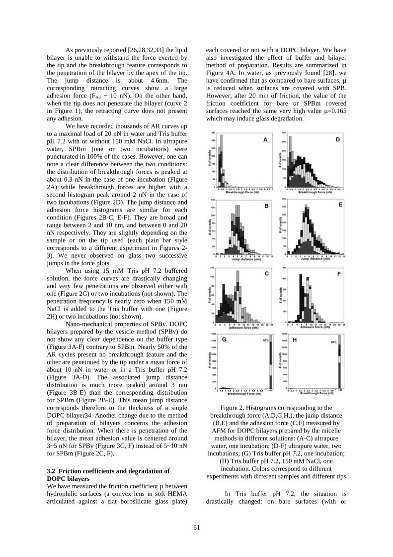
61
As previously reported [26,28,32,33] the lipidbilayer is unable to withstand the force exerted bythe tip and the breakthrough feature corresponds tothe penetration of the bilayer by the apex of the tip.The jump distance is about 4.6nm. Thecorresponding retracting curves show a largeadhesion force (FAd ~ 10 nN). On the other hand,when the tip does not penetrate the bilayer (curve 2in Figure 1), the retracting curve does not presentany adhesion.
We have recorded thousands of AR curves upto a maximal load of 20 nN in water and Tris bufferpH 7.2 with or without 150 mM NaCl. In ultrapurewater, SPBm (one or two incubations) werepuncturated in 100% of the cases. However, one cannote a clear difference between the two conditions:the distribution of breakthrough forces is peaked atabout 0.3 nN in the case of one incubation (Figure2A) while breakthrough forces are higher with asecond histogram peak around 2 nN in the case oftwo incubations (Figure 2D). The jump distance andadhesion force histograms are similar for eachcondition (Figures 2B-C, E-F). They are broad andrange between 2 and 10 nm, and between 0 and 20nN respectively. They are slightly depending on thesample or on the tip used (each plain bar stylecorresponds to a different experiment in Figures 2-3). We never observed on glass two successivejumps in the force plots.
When using 15 mM Tris pH 7.2 bufferedsolution, the force curves are drastically changingand very few penetrations are observed either withone (Figure 2G) or two incubations (not shown). Thepenetration frequency is nearly zero when 150 mMNaCl is added to the Tris buffer with one (Figure2H) or two incubations (not shown).
Nano-mechanical properties of SPBv. DOPCbilayers prepared by the vesicle method (SPBv) donot show any clear dependence on the buffer type(Figure 3A-F) contrary to SPBm. Nearly 50% of theAR cycles present no breakthrough feature and theother are penetrated by the tip under a mean force ofabout 10 nN in water or in a Tris buffer pH 7.2(Figure 3A-D). The associated jump distancedistribution is much more peaked around 3 nm(Figure 3B-E) than the corresponding distributionfor SPBm (Figure 2B-E). This mean jump distancecorresponds therefore to the thickness of a singleDOPC bilayer34. Another change due to the methodof preparation of bilayers concerns the adhesionforce distribution. When there is penetration of thebilayer, the mean adhesion value is centered around3~5 nN for SPBv (Figure 3C, F) instead of 5~10 nNfor SPBm (Figure 2C, F).
3.2 Friction coefficients and degradation ofDOPC bilayersWe have measured the friction coefficient µ betweenhydrophilic surfaces (a convex lens in soft HEMAarticulated against a flat borosilicate glass plate)
each covered or not with a DOPC bilayer. We havealso investigated the effect of buffer and bilayermethod of preparation. Results are summarized inFigure 4A. In water, as previously found [28], wehave confirmed that as compared to bare surfaces, µis reduced when surfaces are covered with SPB.However, after 20 min of friction, the value of thefriction coefficient for bare or SPBm coveredsurfaces reached the same very high value µ=0.165which may induce glass degradation.
Figure 2. Histograms corresponding to thebreakthrough force (A,D,G,H,), the jump distance(B,E) and the adhesion force (C,F) measured byAFM for DOPC bilayers prepared by the micellemethods in different solutions: (A-C) ultrapure
water, one incubation; (D-F) ultrapure water, twoincubations; (G) Tris buffer pH 7.2, one incubation;
(H) Tris buffer pH 7.2, 150 mM NaCl, oneincubation. Colors correspond to different
experiments with different samples and different tips
In Tris buffer pH 7.2, the situation isdrastically changed: on bare surfaces (with or

62
without 150 mM NaCl) the friction coefficient isstabilized to a lower value µ=0.1; when surfaces arecovered with SPB, the friction coefficient issurprisingly low and stable during prolonged friction(i.e., µ=0.035 for SPBm and µ=0.022 for SPBv)with little effect if any of salt (150 mM NaCl). Thisstability of the friction coefficient value in Trisbuffer is accompanied by very little bilayerdegradation if any at the end of the 50 min frictionperiod as seen by the fluorescence images of thebilayer (Figures 4B-E) This stability is a really newresult as we previously obtained a large increase ofµ and an important degradation in water or in a non-buffered saline solution both by the micelle andvesicle method [28].
Figure 3. Histograms corresponding to thebreakthrough force (A, D), the jump distance (B, E)and the adhesion force (C, F) measured by AFM forDOPC bilayers prepared by the vesicle method in
different solutions: (A-C) pure water; (D-F) pH 7.2Tris buffer. Colors correspond to different
experiments with different samples and different tips
4. DISCUSSION
In this report, we have found a strong pHdependence of the mechanical and tribologicalproperties of DOPC bilayers prepared by the micelleor vesicle method.
First, SPBm are easily punctured in water butnot in a Tris buffer pH 7.2. Such a buffer influencedoes not hold for SPBv. Secondly, the distribution ofjump distances (penetration lengths) is peaked
around 3-4 nm for SPBv but ranges up to 10 nm forSPBm. The first value compares well with thebilayer thickness [34,21] while a distance of 7–8 nmagrees with the thickness of two DOPC bilayers. Itstrongly suggests that, in water and when using themicelle method of preparation, a bilayer is alsopresent on the surface of the AFM tip and that twobilayers are interacting together in the recordedforce-distance curves. This result is in agreementwith previous observations of spontaneous bilayeradsorption on an initially bare hydrophilic AFM tip[21,28] or on the glass sphere of a surface forceapparatus when these surfaces are approached to aDOPC SPBm. Interestingly, such an adsorption wasnever reported for the vesicle method to our bestknowledge.
We never observed two successive jumps inthe force plots on glass. The two bilayers aretherefore punctured simultaneously as found forsurfaces covered by surfactant bilayers [36]. Thefact that the adhesion force in the retracting curvesafter a penetration is twice larger for the micellemethod reflects probably that a larger force isneeded to separate two adsorbed bilayers (micellecase) than a bilayer from a bare surface (vesiclecase).
Figure 4. Effect of the bilayer preparation methodand of the buffer on the tribological behaviour ofDOPC supported bilayers. (A) Average values offriction coefficient are calculated from at least 2
independent experiments. Gray bars represent theinitial value and white bars the final value after 50min of friction (except two measurements stopped
after 20 min because of too large friction coefficientdegrading the glass surface). Error bars indicate
minimum and maximum measured values.Abbreviations: W, water; T, Tris buffer pH 7.2; TS,Tris buffer pH 7.2 with 150mM NaCl; SPBm and
SPBv. (B)-(E) In situ fluorescence visualisations ofthe recorded border of the contact zone showing
some eventual bilayer degradation; (B) is the initialcontrol image (before starting sliding the surfaces)
of a SPBm; the same type of bilayer in water showsa strong degradation in water after 20 min of friction
(C) and slight degradation in Tris buffer pH 7.2within 50min of friction (D); a bilayer prepared with
the vesicle method after 50 min of friction in Trisbuffer pH 7.2 with 150 mM NaCl is not degraded
(E)

63
In water, the lower resistance to tipindentation and the propension to spontaneouslyadsorb to other surfaces during contact for SPBm arecertainly related to the presence of traces ofdetergent DDM. First, because these phenomena arenot observed in the absence of detergent (vesiclemethod) and as secondly because the number ofincubations increased significantly the mean bilayerbreakthrough force. A possible scenario is thatdetergent-lipids interactions in water (but not in Trisbuffer) induce a spontaneous curvature and adestabilization of the bilayer. DOPC is normallyconsidered to form particularly stable flat bilayersbut in the presence of cholesterol, its spontaneousradius of curvature is drastically reduced [37].Cholesterol can even lead to the formation ofnonbilayer structures [38]. The formation of defectson DLPE SPB during repeated scanning of the AFMtip was also reported to be highly pH-dependent andwas explained by the increasing bending energy orfrustration due to the high spontaneous curvature ofDLPE monolayers at low pH11. We believe thatsuch an effect is likely to occur here because of a pHdependence of residual DDM-lipids interactions.
In Tris buffer pH 7.2, SPBm seem moreresistant to normal indentation than SPBv (Figures2G,H, 3D). Actually, the distribution ofbreakthrough forces for SPBv is similar topreviously reported values on mica with the samemethod of preparation [26,33]. The great resistanceof SPBm at pH 7.2 is on the other hand a surprisingresult. However, both kind of SPB are not puncturedby forces equivalent to those used in frictionexperiments (i.e, 0.3 MPa in a normal joint whichcorresponds to about 1nN in AFM experiments)[28].This resistance to nano-indentation is againcorrelated with a weak if any bilayer degradationduring prolonged friction and with a low and stablefriction coefficient. SPBv have slightly betterlubricant properties at pH 7.2 than SPBm, perhapsagain due to the presence of traces of DDM in thelatter case. The friction coefficient with DOPCbilayers remains however nearly an order ofmagnitude larger than DPPC bilayers in the solidphase previously measured [28]. This indicates thatfluid bilayers are intrinsically less lubricant thansolid ones even if they resist to shear and normalstress. Understanding the coupling between lipidmobility and surrounding buffer mobility, along withlocalizing precisely the slip plane seems to be thekey steps toward the understanding of mechanismsof biolubrification by lipid layers.
5. CONCLUSION
We have examined the role of the buffer (pH,ions) and the bilayer preparation method on SPBmechanical resistance and tribological properties.The method of preparation gives very different
properties in water but not in Tris buffer pH 7.2. Inwater, SPBm are especially weak and spontaneouslyadsorb to the other contacting surface. In a buffer pH7.2, bilayers are more resistant to nano-indentationand more stable to prolonged periods of friction thanthose in water. They present also better lubricantproperties. Additional salt (150 mM NaCl) haveexisting but secondary effects on the mechanical andtribological properties of the bilayers.
ACKNOWLEDGEMENT
The authors would like to thank Mr. R.Bougaran of CORNEAL Industrie which providedus the manufacturated HEMA lenses, Mrs. Piednoirfrom LPMCN Lyon and Mr. C. Godeau, from INSALyon for their helpful participation in this work. TheLPMCN team belongs to CellTiss consortium. F.D.was supported by a PROFAS fellowship.
REFERENCES
1. Hills, B.A., 1995, Ann. Biomed. Eng., 23, 112–115.2. Johnston, S.A., 1997, Vet. Clin. North Am.Small Animal Prac., 27, 699.3. Schwarz, I.M., Hills, B.A., 1998, Br. J.Rheumatol., 37, 21–26.4. Hills, B.A., 1989, J. Rheumatol., 16, 82–91.5. Hills, B. A., 2000, Proc. Inst. Mech. Eng. H., J.Eng. Med., 214, 83–94.6. McConnell, H.M., Watts, T.H., Weis, R.M.,Brian, A., 1986, Biochim. Biophys. Acta, 864, 95–106.7. Sackmann, E., 1996, Science, 271, 43–48.8. Richter, R.P., Bérat, R., Brisson, A.R., 2006,Langmuir, 22, 3497–505.9. Mou, J, Czajkowsky, D.M., Zhang, Y., Shao,Z., 1995, FEBS Lett., 371, 279–282.10.Brisson, A., Bergsma-Schutter, W., Oling, F.,Lambert, O., Reviakine, I., 1999, J. Cryst.Growth,196, 456–470.11.Hui, S.W., Viswanathan, R., Zasadzinski, J.A.,Israelachvili, J.N., 1995, Biophysical Journal,68,171–178.12.Benz, M., Chen, N., Israelachvili, J., 2004, JBiomed Mater Res A, 71, 6–15.13.Fang, Y., Yang, J., 1997, J. Biochim BiophysActa, Biomembranes, 1324, 309–319.14.Butt, H.-J., 1991, Biophys.J., 60, 1438–1444.15.Ducker, W.A., Senden, T.J., Pashley, R.M.,1991, Nature, 35, 239–241.16.Dufrêne, Y.F., Boland, T., Schneider J.W.,Barger, W.R., Lee, G.U., 1998, Faraday Discuss.,111, 79–94.17.Mueller, H., Butt, H.-J., Bamberg, E., 2000, J.Phys. Chem., 104, 4552–4559.

64
18.Schneider, J., Dufrene Y.F., Barger W.R., LeeG.U., 2000, Biophys. J., 79, 1107–1118.19.Schneider, J., Barger, W., Lee, G.U., 2003,Langmuir, 19, 1899–1907.20.Butt, H.-J., Franz, V., 2002, Phys. Rev. E., 66,031601.21.Grant, L.M., Tiberg, F., 2002, Biophys. J., 82,1373–1385.22.Loi, S., Sun, G. X., Franz, V., Butt , H.-J.,2002, Experiment. Phys.Rev. E., 66, 031602.23.Richter, R.P., Brisson, A., 2003, Langmuir, 19,1632–1640.24.Künnecke, S., Krüger, D., Janshoff, A., 2004,Biophys. J., 86, 1545–1553.25.Franz, V., Loi, S., Muller, H., Bamberg, E.,Butt, H., 2002, J. Colloids and Surfaces B:Biointerfaces, 23, 191–200.26.Garcia-Manyes, S., Oncins, G., Sanz, F., 2005,Biophysical Journal, 89, 1812–1826.27.Trunfio-Sfarghiu, A.-M., Berthier, Y.,Meurisse, M.-H., Rieu, J.P., 2007, TribologyInternational, 40, 1500–1515.28.Trunfio-Sfarghiu, A.-M., Berthier, Y,Meurisse, M.-H., Rieu, J.P., 2008, Langmuir, 24,8765–8771.
29.Schönherr, H, Johnson, J. M., Lenz, P., Frank,C. W., Boxer, S. G., 2004 Langmuir, 20, 11600-11606.30.Tiberg, F., Harwigsson, I., Malmsten, M. Eur.,2000, Biophys J., 29, 196-203.31.Vacklin, H.P, Tiberg, F., Thomas, R.K., 2005,Biochimica et Biophysica Acta, 1668, 17–24.32.Oncins, G., Garcia-Manyes, S., Sanz, F., 2005,Biophysical Journal, 89, 7373-7379.33.Pera, I., Stark, R., Kappl, M., Butt, H-J.,Benfenati, F., 2004, Biophys. J., 87, 2446–2455.34.Liu, Y., Nagle, J.F., 2004, Phys. Rev. E, 69,040901.35.Leroy, S., Steinberger, A., Cottin-Bizonne, C.,Trunfio-Sfarghiu, A.-M., Charlaix, E., 2009, SoftMatter, 5, 24 p.4997-5002.36.Grant, L.M., Ederth, T., Tiberg, F., 2000,Langmuir, 16, 2285–2291.37.(37). Chen, Z., Rand, R.P., 1997, BiophysicalJournal,73, 267–276.38.Coorssen, J.R., Rand, R.P., 1990, Biochem CellBiol., 68 (1), 65–9.

ISSN 1220 - 8434 ACTA TRIBOLOGICA Volume 18, (2010), 65-76
Simon LE FLOC’H1,2
e-mail: [email protected]
M.C. CORNECI2,3
A.-M. TRUNFIO-SFARGHIU2
M.-H. MEURISSE2
J.-P. RIEU4
J. DUHAMEL2
C. DAYOT2
F. DANG2
M. BOUVIER2
C. GODEAU2
A. SAULOT2
Y. BERTHIER2
1 Université Joseph Fourier, Ecole doctorale
EDISCE, Laboratory TIMC-IMAG, DynaCell
Team, FRANCE2 Laboratoire de Mécanique des Contacts et des
Structures, INSA-Lyon, CNRS UMR5259,
F69621 Villeurbanne Cedex, FRANCE3 Université Technique “Gh. Asachi”, Faculté de
Mécanique, 700050, Iasi, ROUMANIE4 Laboratoire de Physique de la Matière
Condensée et Nanostructures, Université Claude
Bernard Lyon 1, CNRS UMR5586, F69622
Villeurbanne Cedex, FRANCE
IMAGERIE MEDICALE POUR EVALUER LESCONDITIONS DU FONCTIONNEMENTTRIBOLOGIQUES DES ARTICULATIONSSYNOVIALES
Le but de ce travail est d’évaluer avec précision les conditionstribologiques macroscopiques subies par l’articulation du genou aucours de la marche en essayant de considérer les interactions entreelles. Le contexte plus global est la compréhension dufonctionnement tribologique de l’articulation saine lui permettant dedurer 70 ans. Dans une première partie, les vitesses relativestangentielles entre les surfaces en contact ont été évaluées au coursde la marche. L’étude a été consacrée aussi à l’évaluation desconditions géométriques du contact lorsque le pied subit un effortde compression de l’ordre de 300 N (patiente de 29 ans pesant 60kg ayant subi une méniscectomie).Les résultats sur la déformée sont validés qualitativement par deséléments bibliographiques. Ils permettent d’émettre une hypothèsequant à la capacité du cartilage à se déformer de quelques dixièmesde mm suivant son épaisseur sans que la pression locale de contactsoit importante, permettant une répartition de la pression trèsefficace.L’étude a été complétée par l’évaluation de l’influence des effortsmusculaires sur la réaction de contact et sur les déplacementsrelatifs des os (patient de 36 ans et de 62 kg (avec une lésion desménisques) a subi une compression du membre inférieur). Il estconclu que l’action des muscles augmente énormément la pressionmoyenne de contact, mais que cette action peut aussi permettred’optimiser les conditions de contact en déplaçant le tibia parrapport au fémur.Keywords: articulation synoviales, conditions du contact,compression de cartilage
1. INTRODUCTION
L’articulation saine du genou est un systèmetribologique performant car elle peut fonctionnernormalement plus de 70 ans. La compréhension deson fonctionnement tribologique a particulièrementété étudiée dans les dernières décennies car lesmaladies ostéo-articulaires prennent de plus en plusd’ampleur et les traitements ne s’avèrent souvent pasassez efficaces.
De nombreuses études ont montré lefonctionnement complexe des différentescomposantes articulaires prises individuellement(cartilage, synovie et ensemble musculaire) mais lefonctionnement réel d’une articulation dépend nonseulement des propriétés individuelles de chaquecomposant articulaire mais aussi des interactions et
de l’arrangement structurel entre tous cescomposants.
D’où notre intérêt de comprendre lefonctionnement tribologique de l’ensemble del’articulation.
Pour cela des études récentes ont permis dedéfinir un modèle expérimental ex-vivo prenant encompte les caractéristiques physico-chimiques etmécaniques de l’ensemble in vivo cartilage –synovie.
Ce modèle permet de comprendre à l’échellemicroscopique le fonctionnement tribologique del’interaction cartilage – synovie.
En revanche ce modèle comporte desparamètres qu’il faut fixer par rapport aux conditionsréelles du contact (pressions de contact, aires decontact, déformée du cartilage, vitesses relativestangentielles) qui font l’objet de cette étude.

66
2. ETUDE IN VIVO DU MECANISMEARTICULAIRE DU GENOU
Ce travail a été réalisé avec la collaborationavec le Laboratoire de Biomécanique etModélisation humaine (LBMH, Université Lyon 1)et le service d’Arthroscanner de l’Hôpital Lyon Sud.
L'objectif de ce travail est d’évaluer in vivoles conditions tribologiques macroscopiques(pressions de contact, vitesses relatives entre lescartilages articulaires) subies par une articulation dugenou au cours de la marche.
Dans ce domaine, la bibliographie n'apporteen effet que des informations souvent incomplètes,et manquantes d'inter cohérence.
Pour obtenir ces conditions tribologiques,nous avons entrepris une étude englobant: la détermination de la cinématique du contact
(vitesses tangentielles relatives), la mesure de la géométrie du contact
(dimensions et courbures, conformité des corpsen contact, aires de contact),
la détermination de la dynamique du contact: mesures quasi statiques de la déformée des
cartilages articulaires et de la variation del’aire de contact en fonction du chargementarticulaire ;
calculs des efforts musculaires et de laréaction du contact, estimation de lapression,
l’évaluation du rôle musculaire dansl'optimisation des conditions de contact(diminution de la pression de contact par undéplacement relatif des os).
3. STRATEGIE
Nous avons évalué les conditionscinématiques locales, lors de la marche d’unepersonne saine : à partir de données issues de labibliographie (Kapandji ), et d’une base de donnéessur la marche construite au sein du LBMH, dessimulations ont été effectuées en dynamique inverseafin de calculer la « réaction de contact ».
Par imagerie médicale (arthroscanner), nousavons évalué les conditions géométriques locales invivo (courbure des corps en contact, aires decontact) Ces essais ont également permis uneanalyse quasi-statique de la phase d’appui de lamarche, dans le but final d’évaluer la répartition depression en contact.
Deux patients bénévoles ont participé à nosessais quasi-statiques en arthroscanner. Au cours deces essais, nous avons mesuré l’effort extérieurappliqué sur le pied de chaque patient. Nous avonségalement pu enregistrer l’activité électrique desmuscles de l'un des deux patients à l’aide d’undispositif électromyographique.
Ces éléments ont permis de calculer lesefforts développés par les muscles articulaires dugenou, grâce à une évaluation in vivo des bras delevier des muscles et à l’utilisation d’un code decalcul développé au sein du LBMH (thèse en coursd’Alice Bonnefoy).
La mesure du déplacement relatif des os apermis d’étudier le rôle des muscles pourl’optimisation des conditions tribologiques decontact.
Une brève description anatomique du genouest présentée ci-dessous, ainsi qu'un résumé derésultats obtenus dans le cadre de ce travail.
4. ANATOMIE DE GENOU
L’articulation du genou est une diarthrose,c'est-à-dire une articulation mobile, qui comporte(Figure 1):
Deux segments osseux, présentant dessurfaces articulaires. Dans le cas du genou, une desextrémités osseuses est représentée par les condylesfémoraux et l’autre extrémité par le plateau tibial;
Deux cartilages articulaires recouvrant lessurfaces osseuses (cartilage fémoral et cartilagetibial);
La capsule articulaire, fibreuse; La membrane synoviale, qui tapisse
intérieurement la capsule; Des ligaments, reliant les deux segments
osseux (pour le genou il y a 4 ligaments : deuxligaments croisés et deux ligaments latéraux);
Des petites structures fibro-cartilagineuses,les ménisques, qui viennent s’insérer sur les surfacesarticulaires pour assurer une meilleure conformitédes surfaces. L’articulation du genou présente deuxménisques (l'un interne et l’autre externe) attachésau plateau tibial par des petits ligaments;
Une poche graisseuse et des bourses séreuses,sortes de petits coussins hydrauliques constituésd’une enveloppe membranaire contenant un liquidesimilaire au liquide synovial.
Enfin, les tendons des muscles qui s’insèrentà proximité d’une articulation entourent l’ensemblede ces structures. Le rôle principal des muscles estde mobiliser l’articulation, mais ils ont aussi uneimportance pour maintenir la cohésion del’articulation (coaptation).
De nombreux travaux consacrés à l'anatomiepar imagerie médicale ont permis de définir avecexactitude la géométrie des extrémités osseuses encontact. Ainsi, les deux condyles fémoraux formentdes cycloïdes avec des rayons maximaux de 38mmpour le condyle interne et 60 mm pour le condyleexterne (Figure 2.).
En ce qui concerne le plateau tibial, ilprésente deux cavités (glènes) correspondant auxdeux contacts avec les condyles fémoraux. Les deuxglènes ont des rayons d’environ 70mm. Elles se

67
distinguent par leur courbure, la glène interne étantconcave et la glène externe convexe (Figure 3).Cela génère un contact conforme pour le condyleinterne et un contact non conforme pour le condyleexterne.
5. CINEMATIQUE DU GENOU
5.1. Modèle de calcul des vitesses
Pour étudier la cinématique du genou, nousavons utilisé l’hypothèse classique de rattachementferme des ménisques au plateau tibial. Ainsi, lacinématique simplifiée du genou, consiste en lacomposition de deux mouvements entre le condylefémoral et la glène tibiale :
du roulement, influencé par les courbures descorps en contact,
du glissement correspondant à destranslations relatives entre les deuxextrémités osseuses.
Figure 1. Représentation anatomique de l’articulation du genou
Figure 2. Géométrie des condyles fémoraux
Figure 3. Géométrie des glènes tibiales

68
Un modèle géométrique simple a été utilisépour les condyles. Ils sont représentés chacun par unarc de cercle. Le plateau tibial est représenté pardeux segments de droite (Figure 4). Ce modèle, detype cylindre sur plan, permet de quantifierrapidement les vitesses tangentielles entre lessurfaces.
Figure 4. Modèle géométrique de condyle pour lecalcul des vitesses
Selon les conventions de signe utilisées(vitesses positives selon les X positifs), la vitesserelative au point de contact de la surface du cartilaged’un condyle du fémur par rapport à la surface ducartilage du tibia est donnée en prenant le tibiacomme solide fixe de référence. La vitesse relativetangentielle au point de contact du fémur par rapportau tibia est la somme de la vitesse du fémur en cepoint avec la vitesse du point géométrique decontact:
fémur / tibia IV (I) V .R (1)
ou R est le rayon du condyle considéré, VI la vitessedu point de contact I, la vitesse angulaire.
Les valeurs de rayons de courbure retenuescorrespondent à 10° de flexion du genou, et sontissues de l’ouvrage de référence de Kapandji [2]: 55mm pour le condyle externe et 35mm pour lecondyle interne.
Le déplacement des points de contact enfonction de l’angle de flexion, est donné par Li et al.[4] pour le cas des genoux sains en flexion passive.La bibliographie démontre, malgré tout, que lesdéplacements des condyles sont modifiés suivantque le pied est chargé ou non.
Deux vitesses tangentielles sont calculées auxdeux « points de contact ». Enfin, une idée de laréaction du contact articulaire du genou est donnéepar les calculs de dynamique inverse. Cet effortn’est qu’une estimation qualitative de l’effort decontact, permettant d’avoir une idée des conditionsinteractionnelles entre la cinématique et la pressionde contact.
5.2. RésultatsLes résultats des essais sur la cinématique du
genou sont présentés dans la Figure 5.Les vitesses relatives de roulement entre les
surfaces au niveau du contact du condyle internevarient cycliquement de 0 mm/sec à 200 mm/s aucours d’une marche effectuée à 5 km/h. Pendant laphase d’appui, la vitesse relative change deux fois designe et sa valeur maximale dans cette phase est de80 mm / s pour le contact interne et de 130 mm / spour le contact externe. Pendant la phased’oscillation (faibles pressions de contact), lesvitesses relatives sont plus importantes (interne : 200mm / s ; externe : 300 mm / s) et changent égalementdeux fois du signe.
Figure 5. Résultats des essais sur la cinématique du genou

69
Les vitesses de glissement du contact versl’arrière du plateau tibial (25 mm / s au maximum)ne compensent pas les vitesses relatives induites parla rotation du fémur par rapport au tibia car lesrayons de courbure des condyles sont assezimportants. Le condyle externe, dont la surface decontact se déplace plus vers l’arrière que le condyleinterne, a un rayon de courbure supérieur, ce quiaugmente la vitesse relative tangentielle entre lessurfaces en contact à 300 mm/s au maximum.
Ces résultats sont très sensibles aux rayonsdes condyles retenus. Par contre, l’amplitude de latranslation des points de contact vers l’arrière duplateau tibial (de 0° à 60° de flexion), n’influencepas significativement le calcul. Cette translation aune valeur maximale de 10 mm.
6. DINAMIQUE DU GENOU
6.1. Modèle de calcul des déformées des cartilagesarticulaires (fémur et tibia)
La stratégie consiste à évaluer la déformée invivo du cartilage des deux condyles fémoraux enfaisant une différence entre les épaisseurs decartilage mesurées avant et après la compression del’articulation.
Pour obtenir les épaisseurs de cartilage invivo nous avons utilisé le scanner (rayons X) duCHU de Lyon Sud. La technique de scanner utiliséeest nommée « arthro scanner ». Elle comportel’injection intra articulaire d’un produit à base d’iodequi permet de faire ressortir sur des imagesradiologiques les parties cartilagineuses del’articulation. Le volume scanné par les rayons X estde 15 x 23 x 20 cm3 et il permet d’avoir 44 + 77 +66 coupes de genou dans les trois plans du repèreanatomique (Figure 6).
Un montage a été réalisé pour comprimer lemembre inférieur du sujet lors de la prise d’imagespar irradiation X.
Le traitement des deux lots d’images(chargé/non-chargé) a consisté tout d’abord en unereconstitution des volumes du cartilage du fémur.Cette reconstruction a été réalisée en utilisant lelogiciel AutoCAD (Figure 7), et a permis de repérerles zones de contact et mesurer les aires de contactextérieurement chargé ou non. Un recalage spatial, aété nécessaire pour superposer le volume ducartilage comprimé sur le volume du cartilage noncomprimé, en faisant coïncider des points de repèredéfinis sur l'os.
Figure 6. Reconstitution du volume de cartilage en ArthroScanner
Figure 7. Volume du cartilage comprimé,(AutoCAD)
Une carte de la déformée du cartilage dufémur a été ainsi réalisée.
Le calcul de l’effort de contact a été fait enadaptant le modèle de dynamique inverse à notreétude. Ainsi, dans le cadre de notre étude, lesaccélérations sont nulles (quasi statique), et letorseur au niveau du pied se limite à une force àdeux composantes (F impact). Un capteur forcepermet de mesurer les deux composantes de cetteforce sur le pied (suivant X et Y). Le problème estdonc plan, et ne permet que le mouvement deflexion – extension au niveau du genou. Les quatregroupes de muscles inter articulaires du genou lesplus importants pour la flexion – extension sont

70
Figure 8. Modèle de dynamique inverse pour calculer les efforts musculaires et la réaction de contact
inclus dans le modèle : le quadriceps, le bicepsfemoris, le semitendinosus et le gastrocnemius. Lesbras de leviers articulaires sont mesurés in vivogrâce aux images d’arthroscanner. Ces données sontintroduites dans le modèle de calcul en dynamiqueinverse qui évalue les efforts musculairesdéveloppés par le membre inférieur. (Figure 8)
Pour le calcul en dynamique inverse, deuxcritères physiologiques ont été retenus : on minimisela réaction de contact, ainsi que la normequadratique des contraintes des muscles.
Pour vérifier de manière expérimentale si lesmuscles sont contractés ou non, un dispositifélectromyographique a été utilisé.
Par contre, ce dispositif permet seulementd’évaluer de manière qualitative la contracturemusculaire.
Deux patients ont participé à notre étude : Une patiente de 29 ans, pesant 60 kg. Elle n’a
plus de ménisques sur le genou droit, duquelest effectué le scanner. Le fait qu’elle n’aitplus de ménisques augmente lesdéformations. L’effort de compression a étéde 300 N. Nous avons réalisé une carte dedéformées du cartilage du fémur, une analysed’aires de contact fémur - tibia (avant et aprèscompression).
Un patient de 36 ans qui pèse 62 kg. Il a unelésion au niveau des ménisques sur le genougauche où est effectué le scanner, enrevanche, les ménisques sont en très grandepartie sains. L'effort de compression a été de310 N. Pour cette étude, nous avons effectuéun calcul d’effort de contact en prenant encompte l’action musculaire.
6.2. RésultatsLes efforts extérieurs au niveau du pied qui
ont été considérés dans ce travail, avec des vitessesnulles entre les surfaces articulaires et un angle
presque nul entre le fémur et le tibia correspondent àla fin de la phase d’appui de la marche (pointsrouges de la Figure 5).
Dans ces conditions, la pression moyenne auniveau du contact articulaire du genou avecménisques, a été évaluée ente 105 et 106 MPa. On aconstaté que cette pression est augmentée de 50%s'il n’y a pas de ménisques.
De plus, cette étude nous a permis de montrerl’influence des muscles sur les conditions de contactarticulaire, cela est schématisé dans la Figure 6.Ainsi :
Le rôle principal des muscles au niveau d’unearticulation est de générer des couples internespermettant d’assurer le mouvement et/ou l’équilibre.Il a été montré que les efforts externes (poids proprede 40 N et effort de 330 N au bout du pied)appliqués au membre inférieur tendent à réduire laflexion au niveau du genou. Dans ce cas, lesfléchisseurs développent un effort de l’ordre de 1200N pour compenser les efforts externes. Grâce à unenregistrement des efforts musculaires au cours de lacompression de la jambe (électromyogramme), il aété conclu que le quadriceps est également actif.L’activité musculaire du quadriceps n’est cependantpas nécessaire en terme de couple. Cette activité,qu’il nous est impossible de quantifier grâce au codede calcul utilisé pour évaluer l’activité musculairedes autres muscles, doit probablement permettre de« stabiliser » l’articulation. Ainsi, la valeur de 200 Nindiquée Figure 9 (en opposition à 0 N), pourl’action du quadriceps est totalement arbitraire. Plusl’effort du quadriceps est important, plus l’effort desfléchisseurs doit être important pour compenser lecouple interne développé par le quadriceps. Ainsi, siun effort de 200 N est considéré au niveau duquadriceps, l’effort développé par l’ensemble desmuscles fléchisseurs est de 1500 N.
Un rôle secondaire des muscles est demodifier les positions relatives du tibia par rapport

71
au fémur, ce qui provoque une tension du ligamentcroisé postérieur et une compression de la partieantérieure des ménisques. Ce mouvement modifie larépartition de pression et donc les conditions ducontact.
Pour cette étude nous nous sommes placésdans les conditions de fonctionnement défavorables
pour la lubrification articulaire par effets de typehydrodynamique, qui correspondent à la phase situéeentre 15% et 45% du cycle de marche (rectanglejaune de la Figure 5).
Dans cette phase, on peut considérer que lespressions de contact atteignent entre 105 et 106 MPa,avec des vitesses relatives variant de 0 à 5 cm/s.
Figure 9. Schéma d’ensemble du rôle du mécanisme dans les conditions du contact articulaire du genou(Avec ménisques / sans ménisque)
7. CONCLUSIONS
La bibliographie apporte de manière séparéeet de façon incomplète les informations nécessaires àl’étude de la tribologie au niveau de l’articulationsaine du genou. Deux grands buts ont donc étépoursuivis tout au long de cette étude. Le premierbut était de mieux spécifier les conditions de contacttelles que les vitesses de frottement entre lessurfaces de contact, les aires de contact, la pressionde contact, la déformée du cartilage et les effortsmusculaires.
Le second but était de mettre en relation ceséléments qui sont considérés séparément dans labibliographie. En effet, les échelles considéréespour comprendre et analyser les différentsphénomènes vont du mètre (analyse du mouvementd’ensemble comme la marche), au μm (étudetribologique du mécanisme de l’articulation).
Pour synthétiser les apports majeurs de cetravail, trois schémas ont été créés.
Le premier schéma (Figure 9) présente le rôledes différents éléments mécaniques, principalementle rôle des muscles, dans le système tribologiqueconstitué des cartilages et des ménisques (lespremiers corps), du liquide synovial (le troisièmecorps) et l’ensemble des muscles, des os et desligaments (le mécanisme). Il souligne l’importancedu mécanisme de l’articulation sur les conditionstribologiques du contact.
En effet, le premier rôle des muscles auniveau d’une articulation est de générer des couplesinternes permettant d’assurer le mouvement et/oul’équilibre. Ce premier rôle influe sur la pression decontact qui est augmentée de manière considérable.Ainsi, la pression moyenne au niveau du contactentre les cartilages est évaluée à 1,5 MPa. Cettepression est en grande partie issu de l’action des

72
muscles qui compriment l’articulation. Si les actionsdes muscles ne sont pas considérées dans le calculde la pression moyenne, cette pression moyennen’est plus évaluée qu’à 0,33 MPa. Un rôlesecondaire mais très probable des muscles est demodifier les positions relatives du tibia par rapportau fémur, ce qui provoque une tension du ligamentcroisé postérieur et une compression de la partieantérieure des ménisques (ces efforts ne sont pasévalués au cours du cette étude). Ce mouvementmodifie la répartition de pression et donc lesconditions du contact. Dans le cadre de notre étude,les efforts externes (poids propre de 40 N et effort de330 N au bout du pied) appliqués au membreinférieur tendent à réduire la flexion au niveau dugenou. Les fléchisseurs développent un effort del’ordre de 1200 N pour compenser les effortsexternes. Grâce à un enregistrement des effortsmusculaires au cours de la compression de la jambe(grâce à un électromyogramme), il est conclu que lequadriceps est aussi actif. L’activité musculaire duquadriceps n’est pas nécessaire en terme de couple.Cette activité, qu’il nous est impossible à déterminergrâce au code de calcul utilisé pour évaluer l’activitémusculaire des autres muscles, doit probablementpermettre de « stabiliser » l’articulation. Ainsi, lavaleur indiquée de 200 N (en opposition à 0 N), pourl’action du quadriceps est totalement arbitraire. Plusl’effort du quadriceps est important, plus l’effort desfléchisseurs doit être important pour compenser lecouple interne développé par le quadriceps. Ainsi, siun effort de 200 N est considéré au niveau duquadriceps, l’effort développé par l’ensemble desmuscles fléchisseurs est de 1500 N. La pressionmoyenne de contact est alors réévaluée à 2 MPa. Latension dans le ligament croisé postérieur et lacompression de la partie antérieure des ménisquessont alors moins importantes que lorsque lequadriceps est relâché.
Les efforts extérieurs appliqués au niveau dupied sont analogues à ceux rencontrés à la fin de laphase d’appui de la marche. La flexion de la jamben’est alors pas la même, modifiant toutes lesconditions tribologiques étudiées en statique aucours de ce travail. Les vitesses relativestangentielles exposées sur le schéma (Figure 9) sontcelles de la fin de la phase d’appui, ne donnantqu’une indication des sollicitations en cisaillementque le gel synovial subit en fin de phase d’appui. Larépartition de la pression de contact est influencéepar l’action des muscles, mais aussi par les vitessestangentielles relatives entre les surfaces en contact.En effet, l’étude sur les vitesses relativestangentielles au niveau des points de contact permetde conclure à un régime de lubrification de type« squeeze » allié à un régime de type « palier » enfin de la phase d’appui, ces régimes modifiant larépartition de pression en contact. Alliée à lagénération de pression par le cisaillement etl’écrasement du gel synovial, la déformée du
cartilage influe elle aussi sur la répartition depression. Avec une amplitude de 0,9 mm pour desefforts extérieurs proches de ceux rencontrés en finde phase d’appui, la déformée du cartilage ne peutêtre négligée lors de l’étude de la répartition depression.
Les muscles précédemment cités sont activéspar le système nerveux qui détient des informationssur les conditions de contact. Le second schéma(Figure 10) expose les possibles retoursd’informations (jusqu’au système nerveux) sur lesconditions tribologiques du contact exposéesprécédemment. Ainsi, la tension des ligamentsarticulaires (internes et externes), la tension dechaque muscle, l’effort subit par les ménisques (parl’intermédiaire de la membrane articulaire) et lapression de contact (par l’intermédiaire de lapression sanguine des vaisseaux de l’os sous lecartilage) sont connus par le système nerveux. Lesystème nerveux peut en retour contrôler certainsparamètres (déplacements, efforts, douleur si il y ades lésions) grâce à des critères physiologiques qu’ilse fixe. Ce contrôle vient influencer les mesureseffectuées et surtout vient influencer les conditionsprécédemment exposées. Nous l’avons vu danscette étude, les muscles, contrôlés par le systèmenerveux, peuvent modifier de manière importante lesconditions de contact, pour une même positionmacroscopique enregistrée. Pour une même positionstatique (il est sûrement possible d’étendre cetteobservation au cas du mouvement), il est ainsipossible de réduire la pression de contact oud’annuler les efforts dans les ligaments croisés et lapression de contact sur la partie antérieure desménisques.
Ces informations engrangées par l’organismepeuvent aussi avoir des conséquences sur lespropriétés mécaniques du cartilage (moduled’Young, coeff. de Poisson, épaisseur), mais à pluslong terme. Dans la période embryonnaire latransformation du tissu cartilagineux (le modèle d'osembryonnaire) en tissu osseux est déterminée parl’invasion des capillaires sanguins dans le tissucartilagineux (processus d'ossification). Ceprocessus est stoppé au niveau articulaire parl'équilibre entre la pression mécanique exercée auniveau articulaire (par des mouvements articulaires)et la pression de perfusion des capillaires sanguins(exercée dans le processus d'ossification). Cettezone d'équilibre des pressions marque la zone ducontact entre l'os et le cartilage articulaire. Cettezone est spécifique pour chaque individu et elle peutévoluer au cours de la vie en fonction de l'intensitéde l'effort mécanique transmit dans l'articulation(condition physique de chaque individu). Ainsi, lemanque de mouvement diminue l'épaisseur ducartilage articulaire et peut même produire uneossification complète de l'articulation dans le cas demanque de mouvement dans la périodeembryonnaire.

73
Figure 10. Schéma des retours d’informations possibles vers le système nerveux concernant les paramètres dumécanisme de l’articulation. Hypothèses sur les conséquences mécaniques possibles
De part ses ménisques et les formescomplémentaires des surfaces de contact du fémur etdu tibia, l’articulation du genou a une bonneconformité à l’échelle du cm. En effet, lesménisques et les formes complémentaires des os(surtout pour le condyle interne), permettent d’avoirune très bonne répartition de la pression. Lescourbures des surfaces de contact sont alors del’ordre de quelques cm (4 à 8 cm). L’étude ducontact entre les cartilages doit s’intéresser à deséchelles plus petites. A ce niveau, il a été montré auque le cartilage se déforme de manière importante,jusqu’à 0,9 mm de diminution de l’épaisseur lorsd’une compression de l’ordre de 1500 N surl’articulation.
Une hypothèse qui peut expliquer ces fortesdéformations calculées est la structure même ducartilage qui pourrait se déformer de manièreimportante sans développer des pressionsimportantes au niveau de sa surface. Cette hypothèsepermettrait d’accommoder les différences degéométrie entre les surfaces en opposition jusqu’àquelques dixièmes de mm, toujours dans le but derépartir au mieux la pression. Par exemple, auniveau des bords internes des ménisques, le cartilagedu fémur peut se déformer pour s’accommoder à la
marche que représente le bord du ménisque (marchede quelques dixièmes de mm).
A l’échelle du m, prise en compte grâce autravail en cours au sein du LaMCoS sur lacompréhension du fonctionnement tribologiqued’une articulation saine (Ana-Maria Sfarghiu), laconformité du contact est assurée par la formation de« sacs ou de poches » de gel synovial permettantd’assurer une continuité de la pression malgré larugosité du cartilage.
Ces trois échelles différentes concernant laconformité du contact permettent une répartition trèsefficace de la pression de contact, limitant à longterme l’usure (Voir Figure 11).
Un autre aspect de cette étude a étél’exploration de techniques permettant de retirer desinformations grâce aux images du scanner (ou del’IRM). Grâce à ces images, les bras de levier desmuscles, pour une certaine position du membreinférieur, ont été évalués in vivo avec une bonneprécision. L’amplitude de la déformée maximale ducartilage a elle aussi été évaluée in vivo : Cettetechnique permettra dans les années à venir, avecl’amélioration de la résolution des images, deconnaître in vivo et sans perturber le contact lesdéformations de chaque élément de l’articulation.

74
Figure 11. Les trois échelles importantes assurant la conformité du contact pour une articulation saine
ACKNOWLEDGEMENT
Les auteurs remercient vivement MmeLaurence Chèze (LBMH), Monica Cretan, AliceBonnefoy, dr. Xavière Rivière et son équipe deradiologie (Hôpital Lyon Sud), Lionel Lafarge(INSA de Lyon) pour l’aide précieux apporté à cetteétude.
REFERENCES
1. Adriacchi, O. Dyrby, 2005, “InteractionsBetween Kinematics and Loading During Walkingfor the Normal and ACL Deficient Knee,” Journalof Biomechanics, Vol. 38.2. Adriacchi, O. Dyrby, 2004, “SecondaryMotions of the Knee During Weight Bearing andNon-Weight Bearing Activities,” Journal ofOrthopaedic Research, Vol. 22.
3. Ahmed, Burje, 1983, “In-vitro Measurement ofStatic Pressure Distribution in Synovial Joints--PartI: Tibial Surface of the Knee,” J Biomech Eng..4. Bassey et al., 1997, “Relations BetweenCompressive Axial Forces in an InstrumentedMassive Femoral Implant, Ground Reaction Forces,and Integrated Electromyographs from VastusLateralis During Various ‘Osteogenic’ Exercises,”Journal of Biomechanics, Vol. 30.5. Beillas et al., 2004, “A New Method toInvestigate In Vivo Knee Behaviour Using a FiniteElement Model of the Lower Limb,” Journal ofBiomechanics, Vol. 37.6. Bergmann et al., 2001, “Hip Contact Forcesand Gait Patterns from Routine Activities,” Journalof Biomechanics, Vol. 34.7. Brewer Robin, 2002, Reconstitution dufonctionnement du genou naturel et artificiel, DEAau LaMCoS / CHU Lyon Sud.

75
8. Cheng et al., 2001, “The Influence of Insertinga Fuji Pressure Sensitive Film Between theTiobiofemoral Joint of the Knee Prosthesis on theActual Contact Characteristics,” ClinicalBiomechanics, Vol. 16.9. Clair David, 2000, Analyse et modélisation deseffets mécaniques dans le processus d’usure parimpacts / glissements. Application à des contacts degéométrie conforme. Thèse au LMC (actuelLaMCoS).10. Colloud Floren, 2003, Modélisation dynamiquedu rameur lors d’exercices réalisés sur ergomètresd’aviron. Implications pour l’entraînement, thèsedirigée par Laurence Chèze UCB 1.11. Doriot Nathalie, 2001, Modélisation dynamiquedu membre inférieur pour l’estimation des forcesarticulaires et musculaires mises en jeu pendant laphase d’appui de la marche, Thèse UCBL 1 sous latutelle de Laurence Chèze.12. Duda and Taylor et al., 2004, “Tibio-FemoralLoading During Human Gait and Stair Climbing,”Journal of Orthopaedic Research, vol. 28.13. Fleisig et al., 1998, “An Analytical Model of theKnee for Estimation of Internal Forces DuringExercise,” Journal of Biomechanics, vol. 31.14. Freeman et al., 2005, “The movement of thenormal tibio-femoral joint,” Journal ofBiomechanics, Vol. 38.15. Gautier Thomas, 1997, Adaptation du modèled’analyse quantifiée de la marche à l’étude cliniquedes IMC, Laboratoire LBMH – UCB Lyon 1, 2004.16. Glitsch et al., “The Three-DimensionalDetermination of the Internal Loads in the LowerExtremity,” J. Biomechanics, Vol. 30.17. Haut Donahue et al., 2002, “How the Stiffnessof Menisci Attachments and Meniscal MaterialProperties Affect Tibio-Femoral Contact PressureComputed Using a Validated Finite Element Modelof the Human Knee Joint,” Journal of Biomechanics,Vol. 36.18. Hobatho et al, 1998, “In Vivo Determination ofContact Areas and Pressure of the Femorotibial JointUsing Non-Linear Finite Element Analysis,”Clinical Biomechanics, Vol. 13.19. http://catalog.nucleusinic.com: site commerciald’images d’anatomie.20. Huiskes et al., 1997, “An Inverse DynamicsModelling Approach to Determine the RestrainingFunction of the Human Knee Ligament Bundles,” J.Biomechanics, Vol. 30.21. Iwaki et al., 2000, Tibio-Femoral Movement 1:The Shapes and Relative Movements of the Femurand Tibia in the Unloaded Cadaver Knee: Studied byDissection and MRI,” Journal of Bone and JointSurgery, Vol. 82B.22. Johal et al., 2004, “Tibio-Femoral Movement inthe Living Knee. A Study of Weight Bearing andNon-Weight Bearing Knee Kinematics Using‘Interventional’ MRI,” Journal of Biomechanics,Vol. 37.
23. Kapandji, 1965, Physiologie articulaire:schémas commentés de mécanique humaine. 2;Membre inférieur. Maloine.24. Komistek et al., 2004, “Knee Mechanics : AReview of Past and Present Techniques toDetermine In Vivo Loads,” J. Biomechancis, Vol.38.25. Kurosawa, Fukubayashi, Nakajima, 1980,“Load-Bearing Mode of the Knee Joint: PhysicalBehaviour of the Knee Joint With or WithoutMenisci,” Clin Orthop, Jun.26. Li et al., 2004, “In Vivo Tibiofemoral ContactAnalysis Using 3D MRI-Based Knee Models,”Journal of Biomechanics, Vol. 37.27. Lu et al., 1998, “Validation of a Lower LimbModel With In Vivo Femoral Forces Telemeteredfrom Two Subjects,” Journal of Biomechanics, Vol.31.28. Mahfouz et al., “In Vivo Determination of theNormal and Anterior Cruciate Ligament-DeficientKnee Kinematics,” Journal of Biomechanics, 200429. Majumbar et al., 2004, “A Three DimensionalMRI Analysis of the Knee Kinematics,” Journal ofOrthopaedic Research, Vol. 22.30. Maquet, Van de Berg, Simonet, 1975,“Femorotibial Weight-Bearing Areas. ExperimentalDetermination,” J Bone Joint Surg Am., Sep.31. McCarthy et al., 1999, “Knee CartilageTopography, Thickness, and Contact Areas fromMRI: In-Vivo Calibration and In-VivoMeasurements,” Oseoarthristis and Cartilage, Vol.7.32. McPherson et al., 2004, “Imaging Knee MotionUsing MRI, RSA/CT and 3D digitalization,”Journal of Biomechanics, Vol. 37.33. Pandy et al., 1997, “A Musculoskeletal Modelof the Knee for Evaluating Ligament Forces DuringIsometric Contractions,” J. Biomechanics, Vol. 30.34. Pinskerova et al., 2001, The Shapes andRelative movements of the Femur and Tibia in theUnloaded Cadaver Knee: A Study Using MRI as anAnatomic Tool. Chapter 10. In: Insall, J. Scott, W.N.(Eds), “Surgery of the Knee”, Edition Saunders.35. Ramsey et al., Tibiofemoral contact pointsrelative to flexion angle measured with MRI,Clinical Biomechanics, Vol. 17, 2002.36. Rotat François, 2005, Rapport de projet de find’étude effectué au sein du département de l’INSAgenie mécanique et conception.37. Scarvell et al., 2004, “Comparison ofKinematics in the Healthy and ACL Injured KneeUsing MRI,” Journal of Biomechanics, Vol. 38.38. Scarvell et al., 2004, “Evaluation of a Methodto Map Tibiofemoral Contact Points in the NormalKnee Using MRI,” Journal of OrthopaedicResearch, Vol. 22.39. Shelburn et al., 2004, “Pattern of AnteriorCruciate Ligament Force in Normal Walking,”Journal of Biomechanics, Vol. 37.

76
40. Shirazi-Adl et al., 1995, “Biomechanics of theHuman Knee Joint in Compression: Reconstruction,Mesh Generation and Finite Element Analysis,” TheKnee, Vol. 2.41. Shrive, O’Connor, Goodfellow, 1978 ;42. Taylor S.J.G. et al., 2001, “Forces andMoments Telemetred from Two Distal FemoralReplacements During Various Activities,” Journalof Biomechanics, Vol. 34,.43. Thambyah et al., 2004, “Contact Stresses in theKnee Joint in Deep Flexion,” Medical Engineeringand Physics.44. Thambyah et al., 2005, “Estimation of Bone-on-Bone Contact Forces in the Tibiofemoral JointDuring Walking,” The Knee.45. Walker PS, Erkman MJ., 1975, The Role ofthe Menisci in Force Transmission Across the Knee,Clin Orthop.
46. Walsh et al., 1999, “An Improved Method forMeasuring Tibiofemoral Contact Areas in TotalKnee Arthroplasty: A Comprarison of K-ScanSensor and Fuji Film,” Journal of Biomechanics,Vol. 32.47. Wang et Walker, 1974 ;48. Wo et al., 1991, Tibial meniscal dynamics usingthree-dimensional reconstruction of magneticresonance images.49. Woo et al., 1997, “Biomechanics of the ACL:Measurments of In Situ Force in the ACL and KneeKinematics,” The Knee, vol. 5.50. You et al., 2001, “In Vivo Measurement of 3DSkeletal Kinematics from Sequences of BiplaneRadiographs : Application to Knee Kinematics,”IEEE Transactions on Medical Imaging.

ISSN 1220 - 8434 ACTA TRIBOLOGICA Volume 18, (2010), 77-84
M.C. CORNECI1,2
e-mail: [email protected]
A.-M. TRUNFIO-SFARGHIU1
F. DEKKICHE3,4
Y. BERTHIER1
M.-H. MEURISSE1
J.-P. RIEU3
M. LAGARDE5
M. GUICHARDANT5
1 Laboratoire de Mécanique des Contacts et des
Structures, INSA-Lyon, CNRS UMR5259,
F69621 Villeurbanne Cedex, FRANCE2 Université Technique “Gh. Asachi”, Faculté de
Mécanique, 700050, Iasi, ROUMANIE3 Laboratoire de Physique de la Matière
Condensée et Nanostructures, Université Claude
Bernard Lyon 1, CNRS UMR5586, F69622
Villeurbanne Cedex, FRANCE4 Département de Chimie, Faculté de Sciences
exactes. Université Mentouri Constantine (25000),
ALGERIE5 Institut Multidisciplinaire de Biochimie des
Lipides, INSERM / INSA de Lyon, UMR870,
F69621, Villeurbanne, FRANCE
PHOSPHOLIPIDES DANS LE FLUIDSYNOVIAL - INFLUENCE SUR LEFONCTIONNEMENT TRIBOLOGIQUE DESARTICULATIONS SYNOVIALESPATHOLOGIQUES
Des études récentes ont montré le rôle des assemblages lipidiquesassociées à la structure discontinue du fluide synovial dans lesperformances du fonctionnement tribologique d’une articulationsaine. Dans le cas des pathologies articulaire, ce fonctionnementest modifié. Ce travail cherche ainsi à identifier l’influence de lavariation en composition lipidique des fluides synoviauxpathologiques sur le fonctionnement tribologique des articulationssynoviales atteintes de différentes pathologies (arthrite, arthrose)Keywords: biotribology, synovial joints, phospholipids, lipidomicanalysis
1. INTRODUCTION
Les recherches de ces dernières années ontproposé différents types de substances en tant queresponsables (seules ou ayant une action synergique)pour la lubrification au niveau des articulationssynoviales caractérisées par un frottement bas et uneusure réduite. On peut mentionné : l’acidehyaluronique (HA) [1], la lubricine [2-4], lecartilage, qui attire les têtes hydrophiles desphospholipides [5] (en utilisant la chromatographiesur couche mince (CCM), Hills avait conclu que laphpsphatidyl-choline (PC) est le plus abondantphospholipid qu’on trouve sur la surface du cartilagearticulaire en y format des structures empilées [6,7]),les proteoglycans de type PRG4 [8], les SAPLs [2].Ces composants sont synthétisées au niveau defluide synovial par les synoviocites : PGL4 [9],SAPL [2], HA [10], les chondrocites [11].
En tant que fluide biologique, le fluidesynovial est un ultrafiltrate de plasma, concentrée àtravers la membrane synoviale.
L’équilibre (l’homéostasie) entre laproduction des composants de fluide synovial et leurfiltration au niveau de la membrane synoviale assurele comportement tribologique remarquable desarticulations saines, constituant des systèmes ayantune usure réduite et un frottement bas au niveau ducontact articulaire.
Pourtant, dans le cas des pathologiesarticulaires (l’arthrite, l’arthrose ainsi que leremplacement d’une articulation non fonctionnellepar un implant articulaire) on constate uneaugmentation du frottement au niveau du contactarticulaire ainsi que l’usure des surfaces de cartilagequi est accompagnée par une altération descaractéristiques biochimiques du fluide synovial,notamment de sa composition lipidique.
Dans le cas de l’arthrose, l’usure descartilages a été corrélée entre autre avec desdisfonctionnement biologiques dus à l’activation dela phospholipase A2 qui modifie la structuremacromoléculaire du fluide synovial en détruisantses assemblages lipidiques, ce qui modifie leur

78
comportement mécanique et par conséquent celui del’articulation synoviale.
D’autres marqueurs des disfonctionnementsbiologiques (ex. léucotriène de type LTB4 etprostaglandine de type 5-HETE dans les casd’inflammation) ont été identifiés dans l’articulationarthrosique.
Même si les études ont montré que lesphospholipides sont les composants majeurscontribuant à la lubrification au niveau de cartilagearticulaire [14,15], il n’y a pas beaucoup d’études’intéressant à la nature des différentes classes dephospholipides présents au niveau des articulationssynoviales (liées à la surface de cartilage articulaireou bien dans la composition du fluide synovial).Cette étude est donc menée afin d’analyser lecontenu en phospholipides présentes dans différentesclases de fluides synoviaux pathologiques. Descontraintes d’éthique médicale nous ne permettentpas d’avoir accès pour ces études à des échantillonsde fluide synoviaux sains.
Les différentes classes de phospholipides ontété identifiées et quantifiées en utilisant lachromatographie gazeuse (GC) en couplage avec lachromatographie sur couche mince (CCM).
En vingt ans, la pratique médicale a constatéun accroissement des maladies articulaires de plusde 30%. Leurs traitements supposent soitl’utilisation de médicaments soit l’interventionchirurgicale pour mettre en place des prothèsesarticulaires dont la durée de vie in vivo est aumaximum de 10 ans, alors que la durée de vie d’unearticulation saine est d’environ 70 ans.
Des études récentes [12] considèrent quecette différence peut-être due aux conditions d'essaisex vivo, qui généralement ne respectent passuffisamment la réalité biologique complexe. Eneffet la plus parte des pathologies articulaires sonttraitées en essayant d’améliorer les constatscliniques. Si cette démarche donne des résultatsassez satisfaisants pour les pathologies simples, les
résultats satisfaisants sont en nombre limité pour lecas des pathologies complexes au niveau descontacts frottants biologiques et cela parce que dansces cas il y a plusieurs composants qui doivent êtreconsidérés.
Lors d’une pathologie articulaire, c’est tout letriplet tribologique qui est soumis à desdysfonctionnements biologiques. Si cesdysfonctionnements sont à nos jours de mieux enmieux diagnostiqués individuellement, ils en restentencore des difficultés expérimentales in vivo quirendent assez difficile la prédiction de leurs effetscouplés ainsi que l’identification des éléments dutriplet tribologique qu’ils affecteront. Cette situationfait que souvent un traitement n’intervient que surun effet intermédiaire sans même parfois traiter lebon élément du triplet. Pour remédier cette situation,il faut donc optimiser les traitements pour ciblerl’élément du triplet tribologique dans lequel il fautcontrôler la libération du bon principe actif. Pour cefaire, dans cet étude on cherche à reproduire ex vivoles pathologies articulaires afin d’optimiser leurstraitements. Pour cela, on utilise le modèletribologique ex-vivo réaliste [13] qui prend encompte le comportement biologique complexe d’unearticulation (cartilage et fluide synovial) (Figure 1).
Ce modèle a permis de mettre en évidence lerôle des assemblages lipidiques, associés à lastructure discontinue du fluide synovial (Figure 2),qui assurent les performances tribologiques dufonctionnement articulaire sain. De plus, il respecteles structures moléculaires et les interactions entreles éléments du triplet tribologique - cet à dire lemécanisme (le fonctionnement articulaire saine,simplifié avec une vitesse de glissement très faible,permettant d’exacerber le rôle de 3ème corps), les 1ercorps (reproduisant ex vivo les caractéristiques ducartilage articulaire sain (hydrogels type HEMA), etle 3ème corps (reproduisant d’une manière réaliste lastructure et la composition du fluide synovial sain).
Figure 1. Modèle ex vivo réaliste de la lubrification articulaire [12]
Figure 2. Assemblages lipidiques dans la structure discontinue du fluide synovial [12]

79
Dans le cas d’une pathologie articulaire detype arthrite on a une inflammation du fluidesynovial accompagnée d’une baisse locale de pH, cequi favorisent l’augmentation du coefficient defrottement et des endommagements locale quidéterminerons l’usure du cartilage, la principalecaractéristique d’une arthrose qui nécessite pour sontraitement la mise en place d’une prothèse. Vue ceschangements au niveau d’une articulationpathologique on peux distinguer des paramètres desdisfonctionnements pathologiques à introduire dansle modèle ex vivo existant: mécaniques,physicochimiques et biologiques.
Dans ce contexte, l’objectif de ce travail estd’adapter le modèle ex vivo existant en yintroduisant les paramètres biologiques,physicochimiques et mécaniques des pathologiesafin de simuler le fonctionnement pathologique et decomprendre le bon enchaînement cause/conséquenceresponsable d’une pathologie et donc de cibler sontraitement aussi bien médicamenteux(pharmacologie articulaire) que prothétiques(surfaces frottantes des implants articulaires).
Il faudra donc apporter des solutionsd’optimisation des traitements pour différentespathologies articulaires et pour un meilleurfonctionnement tribologique des articulationsprothésées.
2. MATERIEL ET METHODE
Pour arriver à proposer des solutionsd’optimisation des traitements des pathologiesarticulaires il est nécessaire de faire des étudesbiologiques pour déterminer les variations de lacomposition lipidique [13] et la destructiond’assemblages lipidiques par des actionsenzymatiques associés aux pathologies articulaires.
Pour cela, la composition lipidique/biologique « réelle » de ces assemblages lipidiques,dans le cas de pathologies articulaires ou enprésence d’une prothèse ont été déterminées enutilisant des analyses lipidomiques de fluidessynoviaux caractéristiques pour différentespathologies articulaires (collaboration avec l’InstitutMultidisciplinaire de Biochimie des Lipides, INSAde Lyon, France) [16].
a. Lipides analysés : phosphatidylcholine (PC),phosphatidyléthanolamine (PE) et phosphatydil-inozitol + phosphatidil sérine (PI + PS)
Extraction lipidique : On a fait la séparationdes lipides en différentes classes : phospholipides,mono- et di-glycérides, cholestérol, acides graslibres, triglycérides et esters de stérol parchromatographie sur couche mince (CCM) ensuite laséparation des différentes classes dephospholipides : PE, PC, PI, PS. Ensuite, par trans-estérification de ces fractions on a fait l’ analyse de
leur contenu en acides gras par chromatographiegazeuse couplée à la spectrométrie de masse.
b. Lipides médiateurs de l’inflammationL’infiltration des leucocytes entraîne la
formation de leucotriènes et en particulier duleucotriène B4 (LTB4) formé à partir de l’acidearachidonique (20:4n-6). Ce dernier est libéré paractivation de la phospholipase A2 lors del’inflammation et devient substrat de la 5-lipoxygénase pour former les leucotriènes et l’acide5-hydroxy-eicosatétraénoïque (5-HETE). LTB4 et 5-HETE ont été extraits du liquide synovial, puismesurés par chromatographie liquide à hauteperformance (HPLC).
Ces deux marqueurs ont été validités dans denombreux modèles inflammatoires [15-17]. Ilspermettront dans les études cliniques de déterminersi la prothèse est bien acceptée par le patient. Ilspourront aussi être utilisés pour vérifier l’efficacitéde médicaments anti-inflammatoires.
Quatre types de fluides synoviauxpathologiques ont été analysés : fluide synovial suite au décèlement et
remplacement d’un implant articulaire (I) ; fluide synovial dans le cas d’une arthrose
« localisée » (AL) ; fluide synovial dans le cas d’une arthrose
« localisée » accompagnée d’une infection(ALI) ;
fluide synovial dans le cas d’un patientmanifestant une arthrose « généralisée » (AG).
c. Préparation des échantillons biologiques (danschaque éprouvette on a 1 ml fluide synovial)
A l’hôpital, des précautions s’imposent : ilfaut utiliser seulement des récipients en verre, jamaisde « plastique » ; de plus la solubilisation de lasynovie se fait « sur place » dans des éprouvettes enverre contenant chaque une : 3 ml éthanol, 0.15 mldeferoxamine (agent hémolytique, 15µmol final,M=656.79g/mol), 0.5 ml butilhydroxytoluèn - BHT(antioxydant, 5mmol final, M=220.35g/mol) etensuite le transport au laboratoire se fait dans lesplus brefs délais dans une boîte de glace carbonique–20°C). Une fois arrivé au laboratoire on fermesous azote et on stock les échantillons à -20°Cjusqu’au moment quand on continue l’analyselipidomique, cet à dire l’extraction etquantification des lipides;
Extraction lipidiqueLes lipides sont extraits [18] à l’aide d’un
mélange éthanol/chloroforme (3/6, v/v) contenant duBHT à la concentration finale de 5.10-5 M, enmilieu acide (pH = 3) (à l’aide d’acide acétiqueglaciale). On utilise comme standard interne du100µl PC (10mg/ml) et 50µl PE (1mg/ml) ajoutésdans chaque tube.
Les lipides sont extraits selon la méthode deBligh et Dyer (1959) par le mélange

80
chlorophorme/méthanol (1/2 ; v/v) en présence deBHT (5.10-5M). Après fermeture sous azote, vortexet centrifugation (5 min, 25°C, 1800torr/min) lemélange se sépare en deux phases. La phase aqueuseest récupérée et transférée dans un autre tube,ensuite évaporée sous jet d’azote ; une deuxièmeextraction est effectuée el les phases organiquesobtenues sont réunies puis évaporées à sec etconservées sous azote à -20°C. On ajoute denouveau 3ml éthanol et 6 ml de chloroforme etl’échantillon est de nouveau centrifugé ensuite lesurnageant (la phase supérieure) est récupéré et laphase restante est ré extraite 2 fois commeprécédemment.
Séparation par CCM (en phospholipidestotaux, marqueurs d’oxydation)
Les extraits lipidiques (évaporées à sec sousazote) sont reprises dans un faible volume dumélange méthanol/chloroforme (1/2, v/v) (250µl)pour être déposées sur une plaque de silice dechromatographie en couche mince (CCM). Lesstandards de migration sont déposés simultanémentà raison de 10µl LTB4 et 8 µl 9-HODE. Laséparation des lipides est effectuée par migrationdans le système de solvants : n-héxane : diethiléther : acide acétique glaciale (25 :75 :1, v/v/v).Apres la séparation, et le séchage des plaques, larévélation des standards de migration se fait parvaporisation de phosphomolibdate puis chauffage dela plaque à 50°C.
La zone de silice correspondant au dépôt estsituée à la même hauteur que le standard demigration plus 1 cm au dessus et au dessous. Lesbandes de silice correspondant aux phospholipidestotaux et aux marqueurs d’oxydation sont grattées etrécupérées dans des tubes en verre à vis. La silice estréhydratée par un mélange de 2 ml méthanol :chloroforme (2/1) et ensuite 2 fois avec 2 mlchloroforme, pour les phospholipides totaux et 2 foisavec 3 ml méthanol pour les marqueurs d’oxydationafin d’extraire ces composants de la silice. Leséchantillons sont centrifugés (5min, 25°C,1800torr/min). La phase supérieure est récupéréepour préparer la séparation CCM des phospholipidestotaux [19] et de l’autre coté pour préparer leséchantillons pour HPLC (identification desmarqueurs de stress oxydant). Les phases d’intérêtsont rassemblées et évaporées à sec sous azote.
Séparation par CCM (des phospholipides)Les extraits de phospholipides totaux
(évaporées à sec sous azote) sont reprises dans unfaible volume du mélange méthanol/chloroforme(1/2, v/v) (400µl) pour être déposées sur une plaquede silice de chromatographie en couche mince(CCM). Les standards de migration sont déposéssimultanément à raison de 30µl PE (1mg/ml) et 3µlPC (10mg/ml). La séparation des lipides esteffectuée par migration dans le système de solvants :chloroforme : méthanol : méthyle amine aqueuse40% (61 :19 :5, v/v/v). Apres la séparation, et
séchage des plaques, la révélation des standards demigration se fait par vaporisation dedicluorofluoresceine, puis repos 5 min et puisvisualisation en UV. La zone de silice correspondantau dépôt est située à la même hauteur que lestandard de migration plus 1 cm au dessus et audessous. Les bandes de silice correspondant auxphospholipides d’intérêt (PE, PC, PI+PS) sontgrattées et récupérées dans des tubes en verre à vis.
Transmethilation et GC (chromatographiegazeuse)
Les acides gras sont trans méthylés enprésence de 750µl mélange toluène : méthanol (2/3,v/v), 750 µl BF3 14% suite une fermeture sousazote, à 100°C dans une cuve thermostatiquependant 90 min. La réaction est arrêtée en plongeantles tubes dans la glace et en ajoutant 1.5 ml decarbonate de potassium (K2CO3) 10% afin deneutraliser le milieu. Les esters méthyliques d’acidesgras ainsi obtenus sont extraits par 2ml isooctanepestipur ensuite fermeture sous azote. On appliqueune centrifugation (5min, 1800torr/min) et onobtient une séparation tri phasique. La phaseorganique supérieure et récupérée dans des tubes enverre puis évaporation à sec sous jet d’azote.
Les extraits sont repris dans un volumed’isooctane puis analysés par chromatographiegazeuse (GC) (Système de chromatographie enphase gazeuse couplée à la spectrométrie de masse(GC Hewlett Packard Séries 6890, colonne capillairesilice HP-5MS 30m x 0.25mm, gaz vecteur – hélium0.5 bar) [20, 21].
La quantification (en nanomoles) des acidesgras composants les queues hydrophobes dephospholipides est faite à l’aide des standardsinternes (type 17 :0 PC et respectivement 17 :0 PE)qui sont ajoutés dans les échantillons au moment del’extraction lipidique.
3. RESULTATS
Dans le cas de pathologies articulaires, on ades changement locales qui favorisent les rupturespar actions enzymatiques au niveau des structureslipidiques du fluide synovial donnant ainsil’oxydation de phospholipides (PLs) qui entraîneainsi des modifications de la composition de fluidesynovial en fonction de différents types de PLs. Cesmodifications ont été étudiées par une analyselipidomique quantitative.
De l’autre coté, l’oxydation des lipidesgénère des marqueurs d’oxydation lipidique avecdes modifications de la structure (notamment due àla perte des propriétés hydrophiles-hidrophobes desPLs qui assurent la structure discontinue du fluidesynovial sain). La présence de ces marqueursd’oxydations liée à une modification de la structurea été étudiée par une analyse lipidomiquequantitative.

81
Les analyses sur les échantillons de fluidesynovial pathologique nous ont permis d’établir parchromatographie gazeuse (GC) la compositionlipidique du fluide synovial (en fonction du type dePLs ainsi que pour la composition en acides gras,saturés et non saturés, pour chaque PL identifié)(Tableau 1).
Par chromatographie liquide à hauteperformance (HPLC) de mettre en évidence laprésence dans le fluide synovial de deux médiateurslipidiques d’inflammation (Figure 3), associés auxdifférentes pathologiques articulaires (cesmédiateurs produisent la destruction enzymatiquedes assemblages moléculaires du fluide synovial).
Figure 3. Médiateurs lipidiques d’inflammation (HPLC, pics caractéristiques d’adsorption)
Pour les échantillons de fluides synoviauxanalysés, trois classes majeures des PLs ont étéidentifiées : PC, PE, PI+PS. Les quantités moyennesconcernant la composition en acides gras des PLsanalysés sont présentées dans le Tableau 2. Enutilisant les résultats obtenus par GC, on peutconstater que pour les acides gras non saturés l’acideoléique (C18 :1) est le plus abondant acide gras.
Pour le comportement tribologiquearticulaire, la conséquence de cette variabilité de lacomposition chimique des fluides synoviaux étudiéspeux être identifié d’une coté, en fonction de type dephospholipides (ayant des petite ou grosses têtes,chargés ou neutres) quand on peut avoir unemodification de l’accrochage au niveau desassemblages lipidiques et de l’autre coté, en fonctionde type d’acides gras constituant les queuesphospholipidiques. Dans ce cas on distingue unefaible (cas d’acides gras saturés, en phase solide) ouune forte (pour les acides gras non saturés, en phasefluide) mobilité des lipides à l’intérieur de cesstructures et donc une modification de leursrhéologie. Ces modifications locales peuvententraîner des modifications du comportementtribologique pour le cas des articulations synovialespathologiques.
L’analyse des résultats obtenus ne permetd’identifier les variations pathologiques dans le casdes échantillons étudiés :
pour le phospholipide de type PE
On remarque une quantité plus élevée dans lecas « ALI », on a donc + des charges au niveau desassemblages lipidiques du fluide synovial ce quientraîne une modification de l’accrochage ;
De plus, un % supérieur en acides gras nonsaturés (pour « ALI » et « AG ») indique une plusgrande mobilité des structures lipidiques et donc unemodification de la rhéologie
pour le PCOn remarque qu’il est le phospholipide le
plus abondant dans la composition de fluidesynovial ; sa structure (têtes petits et neutres) nedétermine pas des modifications significatives del’accrochage
Il y a un équilibre entre le % en acides grassaturés et celui en acides gras saturés donc, on n’aspas non plus des changements nets des phases desassemblages lipidique et non plus de leurs rhéologie
pour les PI+PSOn remarque une quantité plus élevée dans le
cas « ALI », on a donc + des têtes + volumineusesau niveau des assemblages lipidiques du fluidesynovial ce qui entraîne une modification del’accrochage ;
Pour toutes les échantillons analysées on aobtenu un % supérieur en acides gras saturés, ce quicaractérise une faible mobilité des assemblageslipidiques et donc pas de changements nets de leursphases et leurs rhéologie.

82
Tableau 1. Variation de la composition lipidique des fluides synoviaux pathologiques
a. en fonction de type de phospholipide
Phospholipides « I » « AL » « ALI » « AG »PE (nanomoles)PC (nanomoles)PI+PS (nanomoles)
37434234
53546347
84588356
78472272
b. en fonction des acides gras saturés ou non saturés composant les phospholipides
Phospholipides Acides gras « I » « AL » « ALI » « AG »PEPEPCPCPI+PSPI+PS
Saturés (w%)Non saturés (w%)Saturés (w%)Non saturés (w%)Saturés (w%)Non saturés (w%)
425352466237
375950495940
276848506138
237045535149
Tableau 2. Composition en acides gras de principales classes de PLs présentes dans les fluides synoviaux pathologiques analysés
Acides gras % PC total % PE total %PI+PS total12:0 0,00 0,00 0,0014:0 0,17 0,40 0,10
16:0 DMA 3,95 0,66 0,9616:0 16,33 34,22 25,9416:1 1,10 1,20 0,7017:0 0,00 0,00 0,00
18:0 DMA 3,83 0,21 0,5518:1 DMA 1,23 0,08 0,15
18:0 14,55 16,30 15,6318:1 n-9 11,82 14,29 6,0318:1 n-7 2,46 0,28 0,17
18:2 DMA 0,00 0,00 0,0018:2 n-6 8,05 15,17 4,05
20:0 0,09 0,05 2,0518:3 n-6 0,16 0,03 0,0118:3 n-3 0,14 0,05 0,0420:1 n-9 0,21 0,15 0,0720:2n-6 1,55 0,35 1,1720:3n-9 0,00 0,01 0,0020:3 n-6 1,10 3,45 0,40
22:0 0,17 0,05 6,1820:4 n-6 18,49 9,11 4,48
22:1 0,06 0,02 0,1920:5 n-3 0,52 0,46 0,08
24:0 0,76 0,13 7,7522:2n-6 1,83 0,06 1,6522:4n-6 3,73 0,43 0,4324:1 n-9 0,08 0,04 16,6622:5n-6 0,33 0,11 0,0122:5 n-3 1,93 0,48 0,7522:6 n-3 5,38 2,23 3,82
TOTAL acides grassaturés (%)
32,06 51,15 57,65
TOTAL acides grasnon saturés (%)
58,92 47,90 40,69

83
Le fluide synovial fait l’objet de nombreusesétudes cherchant à identifier les composants quiassurent la lubrification en régime limite (boundarylubrication) [5]. Il est montré dans la littérature queles PLs sont impliquées dans le mécanisme de lalubrification au niveau des articulations [2,12], despoumons [22], du péricarde [5].
Pour le comportement tribologique il est doncfort important d’analyser la lubrification en fonctiondes différents paramètres comme: la longueur deschaînes des acides gras, leurs orientation, les taillesdes têtes hydrophiles des PLs, l’accrochage auniveau des surfaces au niveau du contact etc.
Cette étude se concentre sur la compositionlipidique en PLs, par rapport à leurs chaînes d’acidesgras (longueur et saturation) en utilisant deséchantillons de fluide synovial pathologiques et lestêtes hydrophiles (PC, PE, PI et PS).
Les principales classes de PLs identifiéesétaient : PC (32 %) le composant majoritaire, et PE(20%) et Pi+PS (20%) présentes en quantitéssignifiantes. Sarma et al ainsi que Wüthier et al ontmentionnée des résultats similaires [13, 23].
Les objectifs étaient d’étudier les éventuellesmodifications en composition en fonction de l’étatpathologique du fluide synovial ainsi que de mettreen évidence la présence des marqueurs de stressoxydant dans la composition de fluide synovialpathologique (différentes cas cliniques ont étéétudiés).
Les résultats de cet étude nous ont montré lesvariations de la composition lipidique de différentesfluides synoviaux pathologiques en fonction du typede phospholipide contenu ainsi qu’on fonction desacides gras formant leurs queues phospholipidiques(par analyse en GC et HPCL).
Cela nous permet maintenant de reproduireex-vivo les variations de ces compositions et doncd’étudier par la suite l’influence de ces variations surl’accrochage et sur la rhéologie dans le cas desfluides synoviaux pathologiques, afin de déterminerles modifications du fonctionnement tribologiquearticulaire pathologique.
Par la suite ces résultats nous permettront dereproduire ex-vivo et de manière réaliste, lespathologies articulaires afin de comprendre au coursdes essais tribologiques utilisant ce modèle lesdifférents comportements et l’évolution tribologiquedes assemblages lipidiques en fonction despathologies.
4. CONCLUSIONS ET PERSPECTIVES
L’analyse lipidomique nous a permitd’identifier les variations de la composition et lesmodifications de la structure pour le cas des fluidessinoviaux pathologiques ; on connaît doncmaintenant les paramètres de disfonctionnementspathologiques qui caractérise le modèle ex des
pathologies articulaires. L’exploitation de ce modèleau cours des études ex vivo nous permettra decomprendre l’enchaînement causes (pathologies)conséquences (symptomes) dans le but de proposerdes solutions d’optimisation des traitements pour lespathologies articulaires (médicaments et/ouimplants)
En conclusion, PC (32%), PE (20%), PI+PS(20%) sont les trois principales classes de PLsprésentes dans le fluide synovial pathologique. Avecle PC en tant que constituant prédominant. De plus,cette étude a montré la présence d’un mélange desacides gras au niveau des queues lipidiques des PLsanalysées, avec un % supérieur pour les acides grasnon saturés (59%) par rapport aux acides grassaturés (32%).
En pratique, pour traiter efficacementl’arthrose après avoir identifier chaquedisfonctionnement biologiques, il faut en connaîtreles effets mécaniques et physicochimiques afin depouvoir développer des médicaments capables: d’agir principalement sur l’élément du triplet
tribologique qui est la cause de la pathologie, d’être efficaces dans des conditions
physicochimiques variables, imposées parl’évolution de la maladie.Des études supplémentaires serraient
nécessaires pour avoir une caractérisation détailléede l’interaction des phospholipides au niveau de lasurface de cartilage, permettant ainsi une meilleurecompréhension sur la lubrification et les mécanismesde frottement. Cela pourrait inclure la quantificationséparément des autres espèces moléculaires de typePL, la quantification de la sphingomièline et ducholestérol, sachant que leurs présence influence lamobilité des assemblages moléculaire contenant leslipides, l’orientation des lipides dans les liposomespour avoir une information sur l’orientation auniveau des surfaces d’accrochage, l’étude desinteractions lipides –protéines et la modélisationmoléculaire pour estimer l’assemblage ainsi quel’orientation des PLs au niveau des bicouches.
5. REMERCIEMENTS
Les auteurs veulent remercier au collectif dubloc opératoire « Orthopédie adultes » de l’HôpitalEdouard Herriot (Lyon), pour nous avoir fourni leséchantillons de fluides synoviaux pathologiques tantnécessaires pour mener à fin cette étude.
REFERENCES
1. Hills, B.A., 1998, “Enzymatic Degradation of theLoad Bearing Boundary Lubricant in Joint,” Br JRheumatol, 37, pp. 137-142.2. Schwartz, I.M. and Hills B.A., 1998, “Surface-Active Phospholipide as the Lubricating Componentof Lubricin”, Br J Rheumatol, 37, pp. 21-26.

84
3. Furey, M. J., and Burkhardt, B. M., 1997,“Biotribology: Friction, Wear and Lubrication ofSynovial Joints”, Lubr. Sci., 9, pp. 255–271.4. Furey, M. J., 1997, “Exploring PossibleConnections Between Tribology and Osteoarthritis,”Lubr. Sci., 9,pp. 273–281.5. Hills, B.A., 1984, “Surfactants Identified inSynovial Fluid and Their Ability to Act as BoundaryLubricants”, Ann Rheum Dis, 43, pp. 641-648.6. Hills, B.A., 1990, “Oligolamellar Nature of theArticular Surface”, J Rheumatol, 17, pp. 349-356.7. Hills, B.A., 1989, “Oligolamellar Lubrication ofJoints by Surface Active phospholipid”, JRheumatol, 16, pp. 82-91.8. Schmid, R. et al, 2001, "Alteration of Fatty AcidProfiles in Different Pulmonary SurfactantPhospholipids in Acute Respiratory DistressSyndrome and Severe Pneumonia, Am. J. Crit. CareMed., 163, pp. 95-100.9. Jay, G.D, Britt, D.E., Cha, D.J., 2000,“Lubricin is a Product of MegakaryocyteStimulating Factor Gene Expression by HumanSynovial Fibroblasts”, J Rheumatol, 27, pp.594-600.10. Momberger, T.S., Levick, J.R., and Mason,R.M., 2005, “Hyaluronan Secretion by Synoviocytesis Mechanosensitive”, Matrix Biol, 24, pp.510-519.11. Schumacher, B.L., Block, J.A., Schmid, T.M.,1994, “A Novel Proteoglycan Synthesized andSecreted by Condrocytes of the Superficial Zone ofArticular Cartilage”, Arch Biochem Biophys, 311,pp. 144-152.12. Trunfio-Sfarghiu, A.-M., Berthier, Y.,Meurisse, M.-H., Rieu, J.-P., 2007, “MultiscaleAnalysis of the Tribological Role of the MolecularAssemblies of Synovial Fluid. Case of a HealthyJoint and Implants”, Tribology International, 40, pp.1500-1515.13. Sarma, A. V., and Powell G. L., 2001,“Phospholipid Composition of Articular CartilageBoundary Lubricant”, Journal of OrthopaedicResearch, 19, 671-676.
14. Blewis, M. E. et al, 2007, “Model of SynovialFluid Lubricant Composition in Normal and InjuredJoints”, European Cells and Materials, 13, pp. 36-3915. Gale, L.R., Chen, Y., Hills, B.A., CrawfordR., 2007, “Boundary Lubrication of Joints”, Actaortopedica, 78, pp. 309-314.16. Bordet J.-C., Guichardant M., Lagarde M.,1990, “Modulation of Prostanoid Formation byVarious Polyunsaturated Fatty Acids DuringPlatelet-Endothelial Cell Interactions”,Prostaglandins Leukot Essent Fatty Acids, 39, 197-202.17. Corneci M.C. et al., 2007, "Optimisations dessurfaces frottantes des implants articulaires pourfavoriser la lubrification par les assemblageslipidiques", 34TH LEEDS-LYON SYMPOSIUMON TRIBOLOGY – SUMMER SCHOOL, Lyon.18. http://www.cyberlipid.org/19. Wolff, J.P., 1968, "Analyse des lipides etséparation des acides gras par CCM"20. Benzaria, A., 2006, Etude biochimique etnutritionnelle de l'effet immunomodulateur deshuiles de poisson, d'olive et d'argan. Effetscomparés de leurs acides gras, Thèse : InstitutNational des Sciences Appliquées de Lyon,[26/02/2007], p. 105-106.21. Goerke J, 1998, “Pulmonary Surfactant:Functions and Molecular Composition”, Biochim.Biophys. Acta, 1408, pp. 79–89.22. Soares, A.F., 2005, Effets du stress oxydant surle fonctionnement des adipocytes : adiponectine etprostaglandines [En ligne]. Thèse : Institut Nationaldes Sciences Appliquées de Lyon, 2005[04/05/2006], 130 p. Disponible sur :http://docinsa.insa-lyon.fr/these/pont.php?id=soares23. Wüthier, R.E., 1968, “Lipids of MineralizingEpiphyseal Tissues in the Bovine Fetus”, Journal oflipid research, 9, pp. 68-78.

ISSN 1220 - 8434 ACTA TRIBOLOGICA Volume 18, (2010), 85-88
Ionut Cristian ROMANUemail: [email protected]
Emanuel DIACONESCUemail: [email protected]
Department of Applied Mechanics,
University “Stefan cel Mare” of Suceava,
ROMANIA
BIOARTICULAR FRICTION
The present paper illustrates experimental investigations ofbioarticular friction. The first set of experiments was conducted ona pig synovial joint and the second one investigates the frictionbetween a spherical cap made out of cartilage and an elastic half-space. For the experimental investigations, a device was conceivedand built that ensures rolling and sliding movements of the joint.Keywords: bioarticular friction, friction coefficient, synovial joints
1. INTRODUCTION
The human body contains 143 joints thatconnect skeletal bones [1]. Most of these joints aresynovial and represent the object of present study.Human synovial joints are subjected to various andlarge forces under static and dynamic loading, whileexecuting sliding and rolling movements [2].
A joint represents the connection betweentwo or more bones, via a fibers and ligaments.Viewed from the mechanical engineer’s perspective,joints can be treated as cinematic couplings. Ahealthy joint must ensure a series of functions suchas [3]:
allowing bone movements in particulardirections;
ensuring low friction between contactingsurfaces;
receiving and transmitting forces; shock and vibration damping.
2. JOINT TYPES
The first to classify the joints into categorieswas Bichat [1]. Using physiological characteristicsas a criterion, Bichat suggested that joints are eithermobile joints (later named diarthrosis by Galien ) orfixed joints (also named synarthrosis). Another typeof joint can be distinguished, having less mobility,also called amphiarthrosis.
3. EXPERIMENTAL SET-UP
Experimental investigations were conductedon a joint from an approximately 250 days old pig.For preservation, the joint was kept in a containerfilled with 0.98% saline solution, at constanttemperature and in darkness.
Figure 1. Types of joints: a) Synarthosis, [2];b) Diarthrosis, [2]; c) Amphiarthrosis, [4]
Mechanically, the joint was clamped on anadjustable arm at one end and to a stiff enoughelastic lamella at the other. The elastic lamella isrigidly bound to the mobile core of an electro-dynamic actuator. Once the actuator is turned on,the joint is subjected to both rolling and slidingmovements.
Besides the mechanical part, ensuring jointmovements, as shown in Figure 2, the experimentalset-up consists of the following auxiliarycomponents: signal generator, audio amplifier, strainindicator, oscilloscope and PC.
The devices used in the experimentalinstallation are connected one to another asillustrated in Figure 3.

86
Figure 2. Experimental set-up [6]
Figure 3. The connections between devices
The first step of presented experimentalinvestigations was calibration of the measuringdevices. To this end, the strain indicator was firstset to indicate „0” when subjected no load, and asinusoidal signal with a frequency of 3 Hz and anamplitude of 0.8V was programmed at the signalgenerator’s output. In order to quantitatively assessforces transmitted in joints, the elastic lamella wasloaded using dead weights of known mass. Thevalues indicated by the strain indicator are presentedin Table 1.
After calibrating the measuring apparatus, thejoint was fixed into position on the device asdescribed before, and measurements were takenunder different conditions.
Table 1. Loading device calibration values
Weight[g]
Strainindicator
value[mV/V]
Equivalentload [N]
5 0.002 0.0510 0.004 0.120 0.007 0.225 0.008 0.2530 0.01 0.350 0.016 0.5
100 0.031 1150 0.046 1.5200 0.061 2
Experimental measurements of friction weremade for several different frequencies, in the form ofoscilloscope graphical charts, as the one illustratedin Figure 5.
In order to calculate joint friction, the 2Hzchart was considered. This frequency correspondsto a 1.80m tall man having an average step width of0.8m / step, at a frequency of 2 steps / s. This meanshe would walk at a speed of 1.6m / s or 5.7 km / h,which represents the average speed at which anormal human is moving most of the time.

87
Figure 4. Joint clamped on the experimentalapparatus [6]
Figure 5. Friction curve at 2Hz
The graph in Figure 5 indicates that peak topeak signal amplitude is 410mV, and 205mV for ahalf alternation respectively. By comparing thecharts with values obtained when the device wasstatically loaded for calibration, it is shown that for a1N load, an output voltage of 220 mV is generated.In this manner, it is possible to graphically concludethat maximum joint friction occurs when the signalreaches a maximum. For such maximum the forcecan be evaluated as shown in eq. (1):
f1 205
F 0.931N220
. (1)
Thus, for a 2 Hz frequency, the friction forceevaluated at 0.931N. This measured force is theresult of both cartilage friction and loss due tofriction between articular tissue linings.
To better assess friction force between boneends in a joint, a second experimental rig describedin [6, 7] was employed to study the contact betweena bone end and a flat glass surface. Theinvestigations are based on contact mechanicstheory, according to which the contact between twospherical punches (bone ends in this case) can bereplaced by the contact of an equivalent punchpressed against a half-space (represented by theglass plate).
Figure 6. Second experimental set-up [7]
The second experimental set-up consists of amechanical part that ensures loading and movementof the bone pressed against a glass plate, strainindicator, oscilloscope and PC.
As before, the test rig was first calibrated,obtaining for the elastic lamella used in frictionmeasurements a calibrating curve as the one shownin Figure 7.
0 0.5 1 1.50
0.2
0.4
F
u
Figure 7. Elastic lamella calibration curve
In the experimental investigations, thefollowing steps were covered:
Cleaning the glass disc; Connecting the experimental device to the
power supply and strain indicator; Interfacing oscilloscope and strain indicator; Calibrating strain indicator; Equipment functionality was checked before
fixing bone end; Fixing bone end on the support by screw; Lowering the glass disc until contact with
bone end is established. Operating the test rig, thus creating bone end
movements, and recording friction charts as the onedepicted in Figure 8.
The chart in Figure 5 indicates a peak to peaksignal amplitude of 0.8V, value obtained duringcalibrations at a 20 g weight, which corresponds to a0.2N applied force.
In order to validate the experiments, frictioncoefficient was calculated and compared againstliterature values.

88
Figure 8. Friction curve at 15 N loading
Thus, for a friction force of fF 0.02 N at a
N 15 load, the resulting friction coefficient is:
fF0.013
N . (2)
This value was found to be close to frictioncoefficient values from literature.
Another set of tests involved placing waterbetween the bone end and glass plate, thus bettermodeling real life lubrication conditions. A typicalresulting friction curve is shown in Figure 9.
Figure 9. Friction curve (with water lubrication)
According to the chart, signal amplitude is0.6V, which corresponds to a static load of 0.15N,leading to a friction coefficient value as follows:
fF0.01
N . (3)
From these results it can be concluded that, inthe presence of a lubricating layer (in this casewater), friction decreases up to 70% from its initialvalue. Water was chosen as lubricant becausesynovial fluid is 90% water.
4. CONCLUSIONS
The work reported here can be summarizedby a few conclusions listed below.
The first experiment aimed to determine jointfriction without separating joint elements. Severalmeasurements were taken at different frequenciesand friction force was calculated at 2 Hz, frequencycorresponding to a 1.8 m tall man walking at 5.7kmper hour. For these conditions, a friction force of0.931N was determined in the joint.
At first glance, such friction value may seemhigh, but this value includes the friction betweencartilage covered bone ends and that between tissueslining the joint.
Graphical results show an increase in frictionwith frequency, which can be attributed to intra-articular fluid viscosity.
For a better assessment of friction, a secondtest rig was employed, in which cartilage coveredbone ends moves against a flat glass surface. Fromthis second experiment, friction forces wereevaluated at 0.2 N for dry contact and at 0.15N whena liquid (water) was used as lubricant respectively.
On the second rig, measurements were takenat the same frequency (given by the motor drive ofthe device), but contact load varied.
A linear dependence of friction to load wasobserved.
In order to validate obtained results, frictioncoefficients were calculated and found to be in goodagreement with literature values.
REFERENCES
1. Bichat, X., 1829, Anatomie descriptive, JSChaudé, Paris, tome II, pp 41-442. Merkher, Y., Sivan, S., Etsion, I. , Maroudas,A., Halperin, G., Yosef, A., 2006, A RationalFriction Test Using a Human Cartilage on CartilageArrangement, Parma.3. Diaconescu, E., Glovnea, M., Bejinariu, B.,2008, “Experimental Evidence Upon ContactBehavior of Cartilage Covered Bone Ends,”Proceedings of VAREHD 14, Suceava;4. Furey, M.J., 1996, “Friction Wear andLubrication of Natural Synovial Joints,” Proc. Of12th int. Colloquium on Tribology, 1421-1430,Esslingen.5. Diaconescu, E., Glovnea, M., Frunza, G.,2007, Metode inovative de bio-ortopedie pentrureconstrucţia articulară, (in Romanian), contractCEEX BIOART Nr. 70 / 2006, Suceava.6. Romanu, I., 2009, Bioarticular friction, (inRomanian), Graduation Paper, University ofSuceava.7. Brînduşa, B., 2008, Experimental modeling ofbioarticular contacts, (in Romanian), GraduationPaper, University of Suceava.

ISSN 1220 - 8434 ACTA TRIBOLOGICA Volume 18, (2010), 89-105
A.-M. TRUNFIO-SFARGHIU1
e-mail: [email protected]
M.C. CORNECI1,2
Y. BERTHIER1
M.-H. MEURISSE1
J.-P. RIEU3
1 Laboratoire de Mécanique des Contacts et des
Structures, INSA-Lyon, CNRS UMR5259,
F69621 Villeurbanne Cedex, FRANCE2 Université Technique “Gh. Asachi”, Faculté de
Mécanique, 700050, Iasi, ROUMANIE3 Laboratoire de Physique de la Matière
Condensée et Nanostructures, Université Claude
Bernard Lyon 1, CNRS UMR5586, F69622
Villeurbanne Cedex, FRANCE
MECHANICAL AND PHYSICOCHEMICALANALYSIS OF THE TRIBOLOGICALOPERATION OF JOINT REPLACEMENTS
The aim of this work is to identify the coupled role of the biologicalcomponents of synovial fluid in the remarkable tribologicaloperation of a healthy natural joint, as well as in the friction of steeland polythene implants. It uses a realistic ex-vivo model capable ofreproducing the mechanical and physicochemical characteristics ofthe entire tribological triplet of the joint, whether healthy orimplanted. It particularly focuses on the lipidic bilayers and vesiclestructures associated with synovial fluid. The analysis of thefriction measurements and fluorescence microscopy images confirmthe role of lipidic bilayers in maintaining a very low frictioncoefficient. In addition, we observe that the substitute cartilagefavours the formation and maintenance of these bilayers, which isnot the case of implant materials.Keywords: synovial joint, biolubrication, molecular assemblies,lipidic bilayers, articular cartilage
1. INTRODUCTION
Over the years the growing number of osteo-articular diseases has led to the development of jointimplants whose lifetimes depend on theirtribological performances. In spite of sustainedefforts to develop new biomaterials, the in-vivolifetime of implants has often proven to be mostdeceptive when set against extrapolations performedon the basis of ex-vivo simulations. Thisdiscordance can be imputed mainly to ex-vivotribological test conditions that are insufficientlyrealistic in comparison with the mechanical andphysicochemical conditions of biologicalenvironments.
This is why interest has grown over the lastfew decades in attempting to identify andcharacterise the biomolecular interfaces formedduring the tribological operation of healthy andimplanted joints. Thus four biological componentsof synovial fluid have been identified as beingdecisive in the tribological performances of jointsand certain works have attributed separate roles tothem:
albumin protects against wearing of artificialcartilage [1] and the metal surfaces of joint implants[2],
hyaluronic acid tends to increase the viscosityof healthy synovial fluid [3] at low shear rate. But atthe high shear rates encountered in synovial joints,the effect of hyaluronic acid on apparent viscosity isnot significant [4].
lubricin and other polyelectrolytes attach tothe surface of healthy cartilage and modifytribological conditions under boundary regime [5,6].
phospholipids multilayers play also animportant role in the boundary lubrication regime[7,8].
However, these works have neglected the roleof the multiple interactions between the componentsof the synovial fluid and the bodies in contact duringthe tribological operation of the joint. Recentresearch has suggested the essential tribological roleof such interactions.
Under tribological stress the albumins createreticulations with the hyaluronic acid that modify therheology of the synovial fluid [9].
The association of hyaluronic acid with lipidscan form pocket and tube-like structures filled withhyaluronic acid and surrounded by lipidicmultilayers [10]. Furthermore, it has been shownthat such structures reduce the rheothinning effect ofaqueous solutions of hyaluronic acid [11].
The “vitonectin” part of lubricin can fixlipidic bilayers on articular cartilage while its“hemopexin” part protects them against oxidation[12-14].
The healthy joint is an ultra-highperformance tribological system and an essentialreference for understanding the tribologicaloperation of synovial fluid and thus aiding researchaimed at improving the treatment of joint diseasesand optimising implant design. Consequently, thiswork is based on a realistic ex-vivo model tounderstand the coupled role of the molecular

90
components of synovial fluid involved in theremarkable tribological performances of naturaljoints. It also examines the potential capacities ofthese components to improve the tribologicalperformances of joint implants.
The ex-vivo model proposed here, andpresented in section 2, is designed to reproduce themechanical and physicochemical characteristics ofthe whole tribological triplet, either healthy orimplanted, composed of first bodies in contact(articular cartilage and implant materials), the thirdbody (the synovial fluid with its real biomolecularstructure) which separates the first bodies, andobviously the mechanism (muscle and ligamentsystem) which imposes local loadings. This articlefocuses on the boundary regime under which theeffects of hydrodynamic load carrying capacity arecompletely negligible, and which exacerbates therole played by the interfaces.
The tribological analysis proposed in section3 is based on optical microscopy observation oflipidic interfaces performed under white andfluorescent light, in situ through a transparent firstbody, and after opening the contact. The changes inthe lipidic structures are correlated with the changesof the friction coefficient.
2. EX VIVO MODEL TRIBOLOGICALTRIPLET
This section presents a model of an ex-vivotribological triplet of a natural and implanted joint,with realistic mechanical and physicochemicalparameters. We successively describe the elementsmaking up the tribological triplet: the "first bodies"(substitute cartilage and implant material), the "thirdbody" (substitute synovial fluid), and the"mechanism" (experimental device providingcontact pressures and kinetics). The entireprocedure used to define this experimental model ispresented in [15].
2.1 First bodies
2.1.1 Substitute cartilageTaking samples of cartilage affects the
complexity of its structure and in particular destroysthe collagen membrane on its surface. What ismore, it loses its living properties when subjected tolong-term tribological tests, thereby leading us toseek non-living materials capable of forming asubstitute joint cartilage that corresponds as much aspossible to the mechanical and physicochemicalproperties of real cartilage. Consequently, we turnedto highly hydrophilic polymeric materials likehydrogels, since cartilage contains 80% water involume. These materials are used to repair cartilageinjuries: polyalcohol vinyl (PVA) and hydroxyethylmethacrylate (HEMA) [16,17,18]. Of the latter weopted for the hydrogel HEMA used for corneallenses, since its structure and mechanical propertiesare very close to those of cartilage:
HEMA hydrogel has large methacrylatepolymeric chains reticulated by hydroxy-ethylgroups (Figure 1a) that are hydrophilic due to theirnegative HO- charges. This structure is comparableto that of cartilage which has collagen fibresreticulated by glucidic chains (aggrecan, see Figure1b), that are hydrophilic due to their negative SO3-and COO- charges..
Table 1 highlights the similitude between themechanical properties of HEMA hydrogel after 48hours in physiological solution and articularcartilage.
The first bodies used as substitute for jointcartilage are semi-rigid blanks of HEMA lenses(Corneal, France) whose macro-geometry has adomed part (cf. Figure 1a.), making it possible tolocalise the contact during the friction tests. Theroughness of this contact zone is very low (Ra of afew nanometres), comparable to the one of naturalcartilage compressed and flattened to nanometerlevels under the pressures in human hip and kneejoints [19].
a. b.
Figure 1. Schematic representation of hydrogel and cartilage structure: a) hydrogel HEMA (at macroscopic andmolecular scales), b) cartilage (at macroscopic and molecular scales) from [11]

91
Table 1. Mechanical properties of hydrogel HEMA and cartilage listed from literature valuesHydrogel HEMA [21] Cartilage [22]
Equilibrium compressive modulus (MPa) 0.2 – 0.9 0.5 - 1
Permeability (m4/N.s)measured for a gradient of hydrostatic pressure of
21 MPa through 1 mm~ 10-16 10-16 - 10-15
Water content (% mass) ~ 25 %External layer ~ 20 %Internal layer ~70 %
Since this hydrogel reproduces only partiallythe structure and some mechanical properties of thereal cartilage, further on it will be called “artificialcartilage”, following the term of Murakami [20].
2.1.2 Joint implantsTwo types of material used in joint implants
were considered: polyethylene (UHMWPE) andstainless steel (316L). Cylindrical test pieces 15 mmin diameter and 3 mm thick had an RMS roughnessof 0.1 µm for UHMWPE and 0.05 µm for stainlesssteel, representative of the roughness of the rubbingsurfaces of joint implants.
2.2 Model of synovial third bodyThe model of the synovial fluid used in this
study is based on histological and biophysicalobservations showing that synovial fluid formsvesicles (or "pockets") [23] several micrometers indiameter filled with a gel composed of hyaluronicacid and albumins (Figure 2a). According to [10],these "vesicles" are “coated” with lipidic multilayersformed by the stacking of lipidic bilayers and layersof physiological solution that can also be found atthe interface between the synovial gel and thecartilage [8] (Figure 2b).
This type of structure has been reproducedex-vivo by using recent technology derived fromnanostructural physics and described below.
2.2.1 Formation of synovial gel vesiclesSynovial gel was synthesised from DPPC
lipids (1,2-Dipalmitoyl-sn-Glycero-3- Phopho-
choline, 850355CP Avanti Polar Lipids), hyaluronicacid (H7630 Sigma-Aldrich) and serous albumin(A1653 Sigma-Aldrich), acquired in powder form,then placed in physiological solution, in order toobtain concentrations equivalent to those of synovialfluid.
Accumulations of lipids due to their very lowsolubility in aqueous solutions were eliminated byusing a technique specific to the fabrication ofliposomes [24]. They first consist in generating twosolutions with identical volumes:
a solution of 3 g/l lipids in a solventcomposed of 90% chloroform and 10%ethanol in volume,
a solution of 3 g/l hyaluronic acid and 20 g/lserous albumin in physiological solution.The gel vesicles are then formed by following
the procedure schematized in Figure 3, whosesuccessive steps are as follows:
evaporation of the solvent in nitrogen (Figure3a) and centrifugation of the first solutioncauses the lipids to spread over the internalwall of a glass test tube.
the hyaluronic acid and serous albuminsolution is then added to the test tube and theresulting mixture is subjected to ultrasoundfor 2 minutes to trigger the formation of thevesicles, before leaving them to incubate for48 hours at 45°C so that the vesiclesincorporate the synovial gel (Figure 3b).
a) b) c)Figure 2. Schematic view of the synovial fluid : a) discontinuous structure made up of lipidic pockets filled of
synovial gel (hyaluronic acid + albumine), b) lipidic multilayered structures at the interface between synovial geland cartilage, c) detail of the lipidic multilayered structures fixed on articular cartilage by lubricin

92
Figure 3. Procedure of formation of vesicles of synovial gel: evaporation of solvent to cover lipids on thesurface of the test tube, suspension in synovial gel (hyaluronic acid + albumine), sonication to form small
unilamellar vesicles and incubation to form lipid pockets filled with synovial gel (see methods for more details)
2.2.2 Adhesion of lipidic bilayers on the surface ofthe first bodies
To stimulate ex-vivo the multilayer propertiesof the interface between the first and third bodies ina healthy joint as well as possible (Figure 2b), weinitiated the adhesion of lipidic bilayers on the firstbodies by using a lipidic vesicle fusion method[25,26].
This first entails forming lipidic bilayersseveral hundred nanometres in diameter, bysubjecting an aqueous suspension of 2 g/l lipids toultrasound (at 50W power) for 5 minutes. Thissuspension, diluted ten times, is then used toproduce the lipidic deposit.
As shown in the diagram in Figure 4, thedeposit technique consists in:
leaving the surfaces of the first bodies toincubate for 5 minutes in a diluted suspensionof small lipidic vesicles, to which 2mmol/l ofCa++ ions were added to stimulate thevesicles to adhere and burst on the surfaces ofthe first bodies (Figure 4a),
eliminating the lipidic surplus by rinsing(Figure 4b).This technique permits obtaining model
lipidic bilayers containing Ca++ ions. The workdone by Hills [18, 22] has shown that these ions arealso present in in-vivo lipidic bilayers where theystiffen the bilayer by forming ionic links with thenegative parts (phosphate group) of the lipidic heads(Figure. 4c).
Figure 4. Formation of lipidic bilayers by the vesicle fusion method: a) incubation, adsorption and fusion ofvesicles, b) elimination of the lipidic surplus by rinsing, c) internal structure of lipidic bilayers (from [27])
a. b.Figure 5. Chemical-molecular structure of lipids: a) 1,2-Dipalmitoyl-sn-Glycero-3-Phosphocholine (DPPC), b)
1-Palmitoyl-2-[12-[(7-nitro-2-1,3-benzoxadiazol-4-yl)amino]dodecanoyl]-sn-Glycero-3-Phosphocholine(16:0-12:0 NBD PC)

93
2.2.3 Viewing lipidic structuresMolecular markers were added at 1% molar
concentration in DPPC lipidic powder in order toview the initial structure of the third body and itsevolution during the friction tests. These areNBDPC lipids (Avanti Polar Lipids), whose ends arefluorescent under blue light (Figure 5).
In order to focus the microscope on atransparent interface (lipidic bilayer, glass surface,free surface of a solution of synovial vesicles),focusing was done in white light on the projectionon this surface of the octagonal contour of themicroscope’s field diaphragm. This focusing wasthen kept when changing to blue light to view thefluorescent elements of this interface [28].
Several situations can be observed under bluelight:
If the third body does not contain anyfluorescent elements under blue light, the diaphragmdoes not appear in the image. This is, for example,the case of a glass surface without a lipidic bilayer,or of the free surface of physiological solution(Figure 6a).
If the third body contains fluorescentelements, the images obtained under blue light arecomposed of a clear zone bordered by the octagon ofthe diaphragm. This clear zone can be uniform, asin the case of a glass surface with an intact lipidicbilayer (Figure 6b), or an aqueous solution of smalllipidic vesicles, or reveal details as in the case of asolution of large vesicles of synovial gel (Figure 6c).
2.3 Experimental set-upAn experimental set-up permitting the in-situ
visualisation of the contact was developed (Figure 7)to simulate the tribological operation of the modelarticular contact.
The model first bodies (HEMA, PE and steelsamples) were fixed to the bottom of a tankcontaining the third body to be tested. The tank waslinked to a translation stage by a system of flexibleblades. The translation stage imposed cyclictranslation movements forwards and backwards.
A transparent opposing first body formed thecontact with the upper surface of the model firstbody. Normal load was applied by gravity. Anupright microscope (Leica DMLM) linked to acamera (Leica DC350F) for fluorescent analyticalimaging permitted viewing the contact through theopposing first body. This observation was done in-situ, during friction and could be done under whiteand blue (fluorescence) light. Exactly the samecamera acquisition parameters were used under bluelight to compare the different quantities offluorescent lipids in the contact.
An eddy current position sensor measured thedeformation of the flexible blades holding the tank,and permitted calculating the tangential force andthe friction coefficient. The sensitivity, linearityrange and sensor position were set-up so that theuncertainty on the force measurements between -1Nand 1N was 0.0005N.
a. b. cFigure 6. Fluorescence microscopy images of various lipidic structures containing 1% of fluorescent NBDPCusing blue light. a) glass surface without any lipidic bilayer. b) glass surface with an intact lipidic bilayer (theprojection on the surface of the octogonal contour of the microscope’s field diaphragm is seen). c) solution of
synovial gel vesicles without any lipidic bilayer near a glass surface
Figure 7. Schematic view of the experimental device

94
2.4 Experimental procedureFor the tests presented in this text, normal
load was applied at 2.5N, which, by using the curveradii of the test pieces, permitted imposing realisticpressure conditions. The position sensor thusallowed the indirect measurement of frictioncoefficients up to 0.4, with an uncertainty in theregion of 0.0002.
Back and forth displacements were made at aconstant speed of 0.6 mm/s. On the one hand, thislow value permitted good visualization of thecontact by the optical microscope and, on the other,a boundary type lubrication regime. The back andforth movements were of equal duration, in theregion of ten seconds, which, given the speed,permitted the successive visualization of the wholelength of the contact.
Several series of friction tests, each lasting 1h(about 180 back and forth cycles), were performed.They included 3 types of first body and 4 types ofthird body.
The different combinations of first body,aimed at simulating natural articulations and thedifferent types of implant, were the following:
A contact between a convex sample (curveradius 8mm) in soft HEMA (Young modulus ofabout 1.5 MPa) hydrated for 48h in physiologicalsolution and a flat glass (borosilicate) opposingsurface (Figure 8a). Given the load applied, thecontact, which had a diameter of 2mm, wassubjected to an average pressure of 0.3 MPa, whoseorder of magnitude seems realistic in comparison tothe operating healthy knee joint in normal gait[29,30]. In what follows, this contact is called"artificial cartilage contact model".
A contact between a flat sample in steel 316Land a transparent convex opposing surface (curveradius 8mm) made of non-hydrated rigid HEMA(Young modulus of about 1 GPa) (Figure 8b). Thiscircular contact of 0.8 mm in diameter was subjectedto an average pressure of 5 MPa, which is realisticfor the operating knee joint implant in normal gait[31]. This contact is referred in what follows as"steel joint implant contact model ".
A contact between a flat polyethyleneUHMWPE sample and a transparent convex glass(borosilicate) opposing surface (curve radius 25.5mm) (Figure 8c). This circular contact of 0.8 mmdiameter bore an average pressure of 5 MPa, whichis realistic for the operating knee joint implant innormal gait [31]. This contact is referred to in whatfollows as "polyethylene joint implant contactmodel".
The following 4 types of third body andinterfaces were used in order to study in uncoupledmode the tribological role of the differentconstituents of synovial fluid:
physiological solution between the firstbodies not covered with lipidic bilayers, referred tohereafter as "3rd body A", considered as thereference 3rd body with respect to the frictionvalues,
a suspension of 2 g/l of small lipidic vesicles(several hundred nm in diameter) in physiologicalsolution, fluorescent under blue light (cf. 2.2.2) andreferred to hereafter as "3rd body B" (fig 9a),
physiological solution between the firstbodies initially covered with lipidic bilayers (cf.2.2.2), referred to hereafter as "3rd body C", (fig 9b),
lipidic pockets filled of synovial gel (cf 2.2.1)between the first bodies initially covered with lipidicbilayers, referred hereafter as "3rd body D" (fig 9c).
3. EXPERIMENTAL RESULTS
3.1 Friction measurementsFigure 10 shows the evolution of the friction
coefficient, at the start of the test and after one hourof operation for the artificial cartilage contact modelin the presence of 3rd body A (physiologicalsolution). The friction coefficient was observed to bevery stable, in the region of 0.035. The rate ofvariation of the friction coefficient during a cycle isrepresentative of the curves obtained for each of thecombinations between the first and third bodies.However, in other configurations, the friction valuechanged through time.
a. b. c.
Figure 8. Model first bodies considered in this study:a) model of natural joint (model 1st body = hydrated HEMA, transparent 1st body = borosilicate glass),
b) polyethylene joint implant contact model (model 1st body = 316L steel, transparent 1st body = rigid HEMA),c) polyethylene joint implant contact model (model 1st body = UHMWPE,
transparent 1st body = borosilicate glass)

95
a) 3rd body A b) 3rd body B c) 3rd body C d) 3rd body D
Figure 9. Schematic view of the third bodies and interfaces considered in the experimentsa) 3rd body A (physiological solution), b) 3rd body B (suspension of small lipidic vesicles in physiological
solution; c) 3rd body C (physiological solution between the first bodies initially covered with lipidic bilayers,d) 3rd body D (lipidic pockets filled of synovial gel between the first bodies
initially covered with lipidic bilayers)
In the case of the artificial cartilage contactmodel, the friction tests were repeated five times, thedispersion on the friction force being 4% of theaverage value. For the implant models, each of thetests was performed twice, resulting in a maximumvariation of 7% on the friction measurement.
All the average values of the frictioncoefficients obtained in this way for the 12 testconfigurations corresponding to the 3 modelcontacts and 4 third bodies (cf. 2.4.) at the start andend of the tests are grouped in Figure 11.
It can be seen that the combination of lipidswith hyaluronic acid and albumins (3rd body D)gives a higher friction coefficient (0.12), whateverthe model contact studied, than 3rd body A.
On the other hand, the comparison of 3rdbodies B and C, in which only lipids are present,without hyaluronic acid or albumin, with 3rd body Agives results as a function of the model contact andoperating time. The following can be observed:
a significant decrease of the frictioncoefficient for the artificial cartilage contact model(0.035 for 3rd body A, 0.005 for 3rd body B after 1hand 0.0015 for 3rd body C);
an initial decrease of the friction coefficientfor the steel joint implant contact model (0.07 for3rd body A, 0.03 for 3rd bodies B and C), but areturn to the initial value after 1h of friction;
an initial increase of the friction coefficientfor the polyethelene implant contact model (0.06 for3rd body, 0.07 for 3rd bodies B and C), followed bya reduction to 0.05 after 1h of friction. However, thisfall is probably not directly correlated with thepresence of lipids in the third body, since it can alsobe observed with 3rd body A.
3.2 VisualizationThe microscopy images of the first bodies
before friction are shown in Table 2. These showthat:
the soft hydrated HEMA surfaces and rigidnon-hydrated HEMA surfaces, as well asthose in steel and glass, permitted thephysicochemical adhesion of a fluorescentuniform lipidic bilayer (cf. 2.2.2)
however, the polyethelene surface did notadsorb the lipidic bilayer.The in-situ images taken during friction are
shown respectively in the first two columns ofTables 3, 4 and 5. The images show:
a zone including the border of the contact forthe artificial cartilage contact model (Table3).
the central zone of the contact for the implantcontact models (Tables 4 and 5), theexperimental set-up and the contactconfiguration (Figure 8b and 8c) did notpermit access to the edge of the contact.
Figure 10. Typical shape of friction curves recorded with artificial cartilage in the presence of 3rd body

96
Table 2. Visualisation using different lights of the different first bodies (1-6) with or without lipids before contact. First bodies were immersed in water to keep the lipidicbilayer integrity. 1a-6a: Visualisation in white light of the surfaces. 1b-6b: Visualisation in blue light of the surfaces without any lipidic bilayer.
1c-6c: Visualisation in blue light of the surfaces with lipidic bilayer

97
Table 3. Visualisation of artificial cartilage contact model; 1-2: in situ before and after friction; 3-4: after contacton both first-body (hydrated HEMA and borosilicate glass). Different third-bodies were investigated: a-b:
third body B (suspension of small lipidic vesicles in physiological solution); c-d: third-body C (physiologicalsolution between the first bodies initially covered with lipidic bilayers); e-f: third-body D (lipidic pockets
filled of synovial gel between the first bodies initially covered with lipidic bilayers). Images were performedwith white light (a,c,e) or with blue light (b,d,f)

98
Table 4. Visualisation of steel joint implant contact; 1-2: in situ before and after friction; 3-4: after contact onboth first-body (316L steel and rigid HEMA). Different third-bodies were investigated: a-b: third body B(suspension of small lipidic vesicles in physiological solution); c-d: third-body C (physiological solutionbetween the first bodies initially covered with lipidic bilayers); e-f: third-body D (lipidic pockets filled of
synovial gel between the first bodies initially covered with lipidic bilayers). Images were performed with whitelight (a,c,e) or with blue light (b,d,f)

99
Table 5. Visualisation of polyethylene joint implant contact; 1-2: in situ before and after friction; 3-4: aftercontact on both first-body (UHMWPE and borosilicate glass). Different third-bodies were investigated: a-b: thirdbody B (suspension of small lipidic vesicles in physiological solution); c-d: third-body C (physiological solution
between the first bodies initially covered with lipidic bilayers); e-f: third-body D (lipidic pockets filled ofsynovial gel between the first bodies initially covered with lipidic bilayers). Images were performed with white
light (a,c,e) or with blue light (b,d,f)

100
0.03 0.03
0.06
0.07
0.035
0.05
0.07
0.035
0.07
0.015
0.05
0.07
0.005
0.07
0.0015
0.05
0.1
0.0015
0.120.120.12
0.1
0.120.12
0
0.02
0.04
0.06
0.08
0.1
0.12
0.14
artificial cartilage model steel UHMWPE
Frictioncoefficient
3rd body A, start value 3rd body A, end value3rd body B, start value 3rd body B, end value3rd body C, start value 3rd body C, end value3rd body D, start value 3rd body D, end value
Figure 11. Friction coefficients at starting and end of each test
They permit observing changes in thedistribution of fluorescence in the contact andpossibly the exterior during friction.
The last two columns of these tables concernthe images of the first bodies at the end of the tests,after opening the contact and rinsing with distilledwater.
In section 3.3 we propose an analysis of thetribological role of the components of the differentthird bodies tested, in each of the model contacts, byusing the correlations between the values andevolutions of the friction coefficients and theevolution of the images in white and blue light.
3.3 Interpretation
3.3.1 Artificial cartilage contact model3rd body B (physiological solution, small
lipidic vesicles)The presence of small lipidic vesicles
(approximately 200 nm in diameter) solution within3rd body B generated quite significant fluorescence(Table 3, image 1b, part on right) provided byvesicles confined in the contact. This fluorescencewas a little less significant than that recorded outsidethe contact (Table 3, image 1b, part on left) since thelipidic vesicles here were not confined in the contactand thus the thickness of the volume visualized wasgreater. After friction of 1h, the contact zoneappeared much less fluorescent (Table 3, image 2b).
The reduction of fluorescence in the volumeof the 3rd body occurred along with the appearanceof fluorescence on the surface of first bodies:uniform fluorescence on the HEMA surface (Table3, image 3b), and accentuated fluorescence on thefriction trace on the glass surface (Table 3, image4b). The lipidic vesicles present in the third body atthe beginning of friction burst under the effect oftribological stresses leading to a lipidic deposit onthe surfaces of the first bodies. This evolution occurswith a reduction of the friction coefficient from0.015 to 0.005.
3rd body C (physiological solution, lipidicbilayers)
As in the case of 3rd body B, thefluorescence inside the contact before friction wasthe same as that observed outside the contact (Table3, image 1d). But contrary to case B, thefluorescence did not evolve significantly duringfriction (Table 3, image 2d).
Visualisation of the rubbing surfaces of thefirst bodies after friction showed that the lipidicsurfaces initially present remained intact (Table 3,images 3d and 4d).
Correlation of these observations with themeasurement of the very low friction coefficient(0.0015) from the beginning to the end of frictionshowed that the lipidic bilayers adsorbed on the firstbodies resisted friction well and were responsible forthe significant reduction of the friction coefficient incomparison to 3rd body B.
These results demonstrated that the presenceof two lipidic bilayers separated by a physiologicalsalt solution layer in the contact area leads to verylow friction. Our very low friction coefficientvalues contradict the hypothesis that lipids layersonly reduce wear but not significantly friction in thehealthy joints [6]. Low friction could be due to thelocation of velocity accommodation, in thephysiological salt solution layer. This type ofaccomodation mode was also suggested by Briscoeet al. [32], but in their experiments, velocityaccomodation was located in the hydratation waterlayer at the substrate/surfactant monolayer interface.In this study the hydratation layer located betweentwo lipidic bilayers is probably thicker resulting in amuch lower friction coefficient (by a factor of 10).
3rd body D (substitute synovial fluid, lipidicbilayers)
The presence of large lipidic vesicles (a fewdozen micrometers in diameter) filled withhyaluronic acid and albumin gel (“synovial gel”) in3rd body D generated uniform fluorescence insidethe contact, but much weaker than outside the

101
contact where it was not uniform (Table 3, image1f). Therefore the large lipidic vesicles of 3rd bodyD did not remain inside the contact, and thefluorescence observed inside the contact was mainlycaused by the lipidic bilayers adsorbed on the firstbodies.
After 1h of friction, we observed the presenceof fluorescent roller-like structures inside the contact(Table 3, lower part of image 2f). The roller-likeappearance of this structure could be favoured by thepresence of “free” synovial gel (not incorporated inthe lipidic vesicles) and, due to the modification ofthe velocity accommodation mode, be responsiblefor the high friction coefficient (0.12). This value issimilar to those obtained by Benz and Istraelachvili[33] who studied the friction of a hyaluronic acid gelfixed (chemically and physically) by a lipidic bilayeron the surfaces in contact of a surface forceapparatus, and show that synovial gel leads to a highfriction coefficient (0.1 – 0.3) in a boundarylubrication regime.
Visualizations of the surfaces of first bodiesafter friction show the presence of fluorescent lipidicvesicles on the HEMA surface (Table 3, image 3f)and slightly fluorescent non-uniform deposits on theglass surface (Table 3, image 4f).
Therefore all the experiments carried out onthe artificial cartilage contact model show that thelipidic bilayers, adhering physicochemically anduniformly to the rubbing surfaces of the first bodiesled to a very low friction coefficient (in the region of0.0015). Although the lipidic bilayers adhere duringfriction, they do not adhere uniformly (more visiblefluorescent trace of friction in image 4b) which mayexplain why the friction coefficient is slightly higher(0.005). However, a much higher friction coefficient(0.12) is obtained if the friction is localised inside alayer of synovial gel and not in the layer ofphysiological solution that separates the lipidicbilayers deposited on the rubbing surfaces.
3.3.2 Steel joint implant contact model3rd body B (physiological solution, small
lipidic vesicles)The fluorescence inside the contact before
friction was uniform (Table 4, image 1b) but hadcompletely disappeared after 1h of friction (Table 4,image 2b). The small lipidic vesicles (severalhundred nanometres) of 3rd body B were thereforein the contact before rubbing, in the same way as forthe artificial cartilage contact model.
Visualisation of the friction surfaces of thefirst bodies after friction showed that:
the trace of friction on the steel surface didnot contain lipids whereas a uniform bilayerwas observed only outside the friction trace(Table 4, image 3b),
the lipids adhered to the HEMA surfaceuniformly (Table 4, image 4b).
The steel surfaces therefore allowed thephysicochemical adhesion of the lipids, but thelipidic bilayers did not resist the tribological stress,explaining the increase in the friction coefficientfrom 0.03 to 0.07 from the start to the end of thetests (Figure 11).
3rd body C (physiological solution, lipidicbilayers)
As expected, the fluorescence inside thecontact before rubbing was uniform (Table 4, image1d), due to the lipidic bilayers deposited on the firstbodies.
The fluorescence lost its uniformity duringthe test (Table 4, image 2d), since the lipidic bilayersloosened from the first bodies and accumulated influorescent agglomerations inside the contact.Visualisations of the surfaces of the first bodies afterfriction also showed the destruction of the lipidicbilayers after friction and the formation of clusters inthe friction traces on the steel (Table 4, image 3d) ason the HEMA (Table 4, image 4d).
The correlation with a variation from 0.03 to0.1 of the friction coefficient during the tests (Figure11) showed that the lipidic bilayers adhering on thesteel surfaces did not resist tribological stress, andtheir destruction caused the friction to increase.
3rd body D (substitute synovial fluid, lipidicbilayers)
The presence of large lipidic vesicles filledwith hyaluronic acid gel and albumin in 3rd body Dgenerated non uniform fluorescence (Table 4, image1f), which shows that the vesicles remain in thecontact, as opposed to the case of artificial cartilage.After 1h friction these vesicles were seen to mergein the contact and form fluorescent clusters (Table 4,image 2f).
Furthermore, the images of the surfaces ofthe first bodies after friction showed:
the presence of a non uniform fluorescentdeposit on the steel surface over the entirefriction surface (Table 4, images 3e and 3f),
the presence of fluorescent and nonfluorescent clusters at the border of thecontact on the HEMA surface (Table 4,images 4e and 4f).These clusters and the deposit could be
caused by the presence of synovial gel notincorporated in the lipidic vesicles during thefabrication of the substitute synovial fluid. Velocityaccommodation by shearing of these residues couldbe the source of the high friction coefficient (0.12),as in the case of the artificial cartilage model (Figure11).
3.3.3 Polyethylene joint implant contact model3rd body B (physiological solution, small
lipidic vesicles)The fluorescence inside the contact zone
before friction was uniform (Table 5, image 1b), but

102
lessened substantially after 1h friction (Table 5,image 2b). The small lipidic vesicles were thereforepresent inside the contact before friction and weremostly ejected from the contact during friction.
The reduction of fluorescence in the contactzone during the test occurred with the appearance offluorescence over the entire surface of the glasscontact, at a level higher than that of the frictiontrace (Table 5, image 4b). On the other hand, thefluorescence of the polyethylene surface remainednegligible (Table 5, image 3b).
This shows that the lipidic vesicles containedin the volume of 3rd body B and not ejected fromthe contact, burst due to tribological stress, with thelipids adhering only to the glass surface, bothspontaneously and due to the effect of friction.
However, the polyethylene surface did notpermit adhesion by the lipids by spontaneousphysicochemical effects or by tribilogical stresseffects. This appears to result in a high frictioncoefficient comparable to that obtained with 3rdbody A (pure physiological solution). The reductionof the friction coefficient at the end of the test (areduction from 0.07 to 0.05) can be explained by thesmoothing of the polyethylene, resulting in increasedshininess of the friction trace (Table 5, image 3a).
3rd body C (physiological solution, lipidicbilayers)
The presence of lipidic bilayers on thesurface generates fluorescence of the contact (Table5, image 1d), but this fluorescence is less uniformthan in the case of the articular contact model (Table3, image 1d) or the steel joint implant contact model(Table 4, image 1d). This is due to the difference ofwettability between the two surfaces in contact(glass, polyethylene) which caused faults in thelipidic bilayers. During friction, the lipids loosenedfrom the surfaces, to form fluorescent clusters insidethe contact (Table 5, image 2d).
Visualisations of the friction surfaces of thefirst bodies after friction showed, as in the case of3rd body B:
the absence of lipids adhering to thepolyethylene surface (Table 5, image 3d) andthe smoothing of the friction trace detectableunder white light due to the shininess of thefriction trace (Table 5, image 3c).
The presence of a high inhomogeneouslipidic bilayer on the glass (Table 5, image4d), with lipidic clusters that did not existbefore friction (Table 2, image 6c).Thus, in the case of the polyethylene joint
implant contact model, the evolution of the contactwas the same, whether the lipids were initially in thevolume of the 3rd body in the form of small vesicles,or in bilayers on the surface of the first bodies,thereby explaining why the change in the frictioncoefficient was the same (Figure 11).
3rd body D (substitute synovial fluid, lipidicbilayers)
The presence of large lipidic bilayers filledwith synovial gel in the third body generated non-uniform fluorescence of the contact (Table 5, image1f), which shows that these vesicles exist initiallyinside the contact zone. After 1h of friction, fusionof the vesicles into fluorescent clusters was observed(Table 5, image 2f).
Visualisations of the friction surfaces of thefirst bodies after friction showed:
the absence of fluorescence for thepolyethylene surface (Table 5, image 3f), andless pronounced shininess in the friction trace(Table 5, image 3e) than in the two previouscases, thereby showing the start of surfacesmoothing.
the presence of clusters of non-uniformfluorescence in the contact zone on the glasssurface (Table 5, image 4f).In this configuration, it therefore seems that
the accommodation of velocity between the surfaceswas mainly ensured by free synovial gel betweenfluorescent clusters within the 3rd body, whichexplains why the same high level of friction wasfound (Figure 11) as for the artificial cartilage andsteel joint implant contacts models. The polythenewas also seen to smoothen during the test, leading toan apparent reduction of the friction coefficient.
4. CONCLUSIONS
An experimental model was used for the ex-vivo reproduction of the tribological tripletsassociated in, respectively, a healthy joint, a steelimplant, and a polyethylene implant. In particularthe aim was to analyse the tribological role of thebiological components of the natural lubricantprovided by synovial fluid, by specifically focusingon lipidic structures.
In order to exacerbate the role played by theinterfaces, experimental conditions were chosen soas to eliminate any hydrodynamic load carryingcapacity effect; therefore third bodies wereconsidered, making it possible to study the influenceof different lipidic structures on friction separately.
The analysis proposed relied on friction forcemeasurements associated with optical microscopyimages of the contact and surfaces. This microscopymade use of fluorescent and white light to detect thelipidic structures.
The study demonstrated that the presence oftwo lipidic bilayers separated by a physiological saltsolution layer in the contact area leads to lowfriction, clearly shown in the case of the artificialcartilage, where it led to a friction coefficient in theregion of a thousandth. On the contrary, it was notsensitive in the case of the model implants:

103
In the case of the artificial cartilage, thelipidic bilayers resisted realistic tribological stresses.In addition, these stresses favoured their formationin the presence of lipidic vesicles. This beneficialeffect of the lipidic bilayers was not observed in theimplant models.
The steel surfaces also favoured the adhesionof the lipidic bilayers, which tends to reduce friction.However, they did not resist tribological stress andwere totally eliminated from the contact after onehour. Also the friction coefficient returned to a highvalue.
The polyethylene surfaces did not permit anyadhesion of the lipidic bilayers. This result appearsto contradict the literature, which states that thepresence of lipids in a steel-polyethylene contactreduces the friction coefficient [24]. A fall in thefriction coefficient during the tests was observed,though it is only correlated to the smoothing effecton the polyethylene surface.
Furthermore, the addition of hyaluronic acidand albumin in the substitute synovial fluid resultedin an increase of the friction coefficient in all thetests performed. This was probably due to thepresence of hyaluronic acid and albumin “free” gel,i.e. not incorporated in the lipidic vesicles. It wasproposed to explain the increase of the frictioncoefficient that large molecules of hyaluronic acidmay bridge the gap between surfaces [6] even in thepresence of lipidic bilayers [34]. Within theframework of this study, we correlated the increaseof the friction coefficient to the formation of therollers containing lipids, which have been visualizedin fluorescence microscopy (Table 3, image 2f).
However, it is probable that the presence offree synovial gel was due to our method of preparingthe initial synovial gel - lipidic vesicle solution,which did not permit the complete incorporation ofthe gel. Indeed, it appears that the process ofincorporating the gel in the vesicles greatly dependson physicochemical conditions (temperature, pH,osmotic pressure, etc.) [19]. Also, thepharmaceutical synthesis of the liposomes includes afinal filtration step aimed at eliminating the free gel.This filtration was not performed in the frameworkof this work.
What is more, it is probable that there is nofree gel in a healthy joint, in which the presence oflubricin ensures the correct formation of lipidicstructures (bilayers, vesicles), by providing anadhesive interface between the lipidic surfaces of thecartilage and the synovial gel.
The situation is perhaps quite different inimplants. This study suggests that the lipidic bilayersare destroyed by friction, thereby permitting theexistence of free gel and increasing friction.Nonetheless, it should be noted that in spite of anincrease in the friction coefficient, the presence offree gel may have a beneficial effect in protectingthe steel surfaces against wear [1].
This study therefore shows that molecularstructures, such as lipidic bilayers, hyaluronic acidand albumin gel, and theirs interactions have adecisive influence on the tribological performancesof the artificial cartilage and the joint implantmaterials operating under boundary regime. Thus itappears vital to take them into account in implantlifetime tests and not use a lubricant composed onlyof physiological solution and albumin, as is mostoften the case.
A means of optimising the rubbing surfacesof joint implants requires improving thecompatibility of the materials with the lipidicbilayers, in order to obtain a low friction coefficientand a lubrication mode similar to that of a healthyjoint. These conclusions agree with the works ofHills [25] which show a stack of 3 to 7 lipidicbilayers on the surfaces of articular cartilage andsuggest that most implant surfaces do not permit theformation of this stacking.
Our results with lipidic multilayers show verylow friction coefficients similar to those obtained forpolyelectrolyte experiments [Klein]; thus futureexperiments should be done in order to properlyidentify the tribological role of these molecules.Also, it was shown that polyelectrolytes such aslubricin have a role of adhesion on the lipidicmembranes ([34,13]) which could modify theirtribological performance. Therefore, futureexperiments should be performed in presence oflubricin and lipidic multilayers.
ACKNOWLEDGEMENT
The authors would like to thank in particular: Mr. G. Vitally of CORNEAL Industrie which
provided the HEMA samples, Pr. L. Cheze, Pr. J.-P. Carret of the
Laboratoire de Biomécanique et ModélisationHumaine (LBMH) of Université Claude Bernard,Lyon 1 for their help in providing understanding ofjoint dynamics, anatomy and articular histology.
Pr. D. Hartmann of the Institut des SciencesPharmaceutique et Biologique de Lyon, UMR MA,for his help in providing understanding of thebiochemistry and morphology of articular molecularstructures.
M. C. Godeau for his helpful participation inthis work.
REFERENCES
1. Sawae Y., Murakami T., 2006,“AnExperimental Investigation of Boundary LubricationMechanism with Protein and Lipid in Synovial JointUsing Total Internal Reflection FluorescenceMicroscopy”, Journal of Biomechanics; Vol. 39(Suppl 1).

104
2. Wimmer MA, Sprecher C, Hauert R, TägerG, Fischer A. 2003, “Tribochemical Reaction onMetal-on-Metal Hip Joint Bearings. A ComparisonBetween In-Vitro and In-Vivo Results,” Wear; 255 :1007–1014.3. Schurz J, Ribitsch V., 1987, “Rheology ofsynovial fluid,” Biorheology, 24(4): 385-994. Dowson, D., and Jin, Z.M., 1987, “An Analysisof Micro-Elastohydrodynamic Lubrication inSynovial Joints Considering Cyclic Loading andEntraining Velocities,” Fluid Film Lubrication—Osborn Reynolds Centenary, Proc. 23th Leeds–LyonSymposium on Tribology, edited by D. Dowson etal., Elsevier, Amsterdam, 1986, pp. 375–386.5. Swann D.A., Silver F.H., Slayter H.S., StaffordW., Shore E., 1985, “The Molecular Structure andLubricating Activity of Lubricin Isolated fromBovine and Human Synovial Fluids,” Biochem J;225: 195-201.6. Jay G.D., Harris D.A. and Cha C.-J., 2001,“Boundary Lubrication by Lubricin is Mediated byO-linked β(1-3)Gal-GalNAc Oligosaccharides,”Glycoconjugate Journal 18, 807–8157. J. Klein, 2006, “Molecular Mechanisms ofSynovial Joint Lubrication”, Proc. IMechE Vol. 220Part J: J. Engineering Tribology, 220, 691-710.8. Schwarz IM, Hills BA., 1998, “Surface-ActivePhospholipid as the Lubricating Component ofLubricin,” British Journal of Rheumatology; 37: 21-26.9. Hills BA., 1989, “Oligolamellar Lubrication ofJoints by Surface-Active Phospholipid”. JRheumatol;16: 82-91.10.Oates KMN, Krause WE, Jones RL and ColbyRH., 2005, “Rheopexy of Synovial Fluid andProtein Aggregation.” Journal of the Royal SocietyInterface; 1-8.11.Pasquali-Ronchetti, 1997, “Hyaluronan–Phospholipid Interactions,” Journal of structuralbiology; 120: 1–10.12.Crescenzia V, Taglienti A, Pasquali-RonchettiI., 2004, “Supramolecular Structures Prevailing inAqueous Hyaluronic Acid and PhospholipidVesicles Mixtures: An Electron Microscopy andRheometric Study,” Colloids and Surfaces A:Physicochem. Eng. Aspects; 245: 133–135.13.Rhee DK, Marcelino J, Baker MA, Gong Y,Smits P, Lefebvre V, Jay GD, Stewart M, WangH, Warman ML, Carpten JD., 2005, “TheSecreted Glycoprotein Lubricin Protects CartilageSurfaces and Inhibits Synovial Cell Overgrowth ofSynovial Cell Growth,” The Journal of ClinicalInvestigation; 115(3): 622–631.14.Schvartz I, Seger D, Shaltiel S., 1999,“Molecules in Focus: Vitronectin,” TheInternational Journal of Biochemistry & CellBiology; 31: 539-544.15.Tolosano E, Altruda F., 2002, “Hemopexin:Structure, Function, and Regulation,” DNA and CellBiology; 21(4): 297-306.
16.Trunfio-Sfarghiu AM, Berthier Y, MeurisseMH, Rieu JP. “Operation Function of a HealthySynovial Joint. Part I: Design of a TribologicalModel by Multiscale Analysis of the Role ofBiological Components”, submitted for publication.17.Broom ND, Oloyede A., 1998, “The Importanceof Physicochemical Swelling in Cartilage Illustratedwith a Model Hydrogel System,” Biomaterials; 19:1179-1188.18. Freeman ME, Furey MJ, Love BJ, HamptonJM., 2000, “Friction, Wear, and Lubrication ofHydrogels as Synthetic Articular Cartilage,” Wear;241: 129-135.19. Covert RJ, Ott RD, Ku DN., 2003, “FrictionCharacteristics of a Potential Articular CartilageBiomaterial,” Wear; 255: 1064–1068.20. Dowson, D., and Jin, Z. M., 1992,“Microelastohydrodynamic Lubrication of Low-Elastic-Modulus Solids on Rigid Substrates,” J.Phys. D, 25, pp. A116–A123.21. K. Nakashima, Y. Sawae, T. Murakami, 2005,“Study on Wear Reduction Mechanisms of ArtificialCartilage by Synergic Protein Boundary FilmFormation,” JSME International Jurnal, series C,vol 48, nr. 4, p 555-56122. Migliaresi C, Nicodemo L, Nicolais L,Passerini P., 1981, “Physical Caracterisation ofMicroporosus Poly (2-Hydroxyethyl Methacrylat)Gels,” Journal of Biomedical Materials Research;15: 307-317.23. Mow VC, Ratcliffe A., 1992, “Cartilage anddiarthrodial joints as paradigms for hierarchicalmaterials and structures.” Biomaterials; 13(2): 67-97.24. Watanabe M, Leng CG, Toriumi H, HamadaY, Akamatsu N, Ohno S., 2000, “UltrastructuralStudy of Upper Surface Layer in Rat ArticularCartilage By “In-Vivo Cryotechnique” Combinedwith Variosus Tratements,” The Clinical ElectronMicroscopy Society of Japan; 33: 16-24.25. Torchillin V, Weissig V., 2003, Liposomes: APractical Approach, Oxford University Press, USA,.26. He L, Dexter A, Middelberg A., 2006,“Biomolecular Engineering at Interfaces,” ChemicalEngineering Science; 61: 989 – 1003.27. Bayerl TM, Bloom M., 1990, “PhysicalProperties of Single Phospholipids BilayersAdsorbed to Micro Glass Beads: A New VesicularModel System Studied by 2H-Nuclear MagneticResonance,” Biophys. J.; 58(2): 357–362.28. Hills BA, Crawford RW., 2003, “Normal andProsthetic Synovial Joints Are Lubricated bySurface-Active Phospholipid. A Hypothesis,” TheJournal of Arthroplasty; 18( 4): 499-505.29. see the Olyumpus microscopy resource center,http://www.olympusmicro.com/primer/anatomy/reflectkohler.html

105
30. Gale LR, Coller R, Hargreaves DJ, Hills BA,Crawford R., 2006, “The Role of SAPL as aBoundary Lubricant in Prosthetic Joints.” TribologyInternational; Available online 18 January.31. Perie D., Hobatho M.C., 1998, “In VivoDetermination of Contact Areas and Pressure of theFemorotibial Joint Using Non-Linear Finite ElementAnalysis,” Clinical Biomechanics 13, 394-40232. Johnson T.S., Laurent M.P., Yao J.Q.,Blanchard C.R., 2003, “Comparison of Wear ofMobile and Fixed Bearing Knees Tested in a KneeSimulator,” Wear 255, 1107–1112
33. Briscoe et al., 2006, “Boundary LubricationUnder Water,” Nature 444, 191-194.34. Benz M, Chen N, Istraelachvili J., 2004,“Lubrication and Wear Proprietes of GraftedPolyelectrolytes, Hyaluronan and Hyalan, Mesuredin the Surface Forces Apparatus.” Journal ofBiomedical Materials Research Part A; 71A(1): 6-15.35. Bruno Zappone, Marina Ruths, George W.Greene, Gregory D. Jay, Jacob N. Israelachvili,“Adsorption, Lubrication and Wear of Lubricin onModel Surfaces: Polymer Brush-Like Behavior of aGlycoprotein,” Biophysical Journal, 2006

ISSN 1220 - 8434 ACTA TRIBOLOGICA Volume 18, (2010), 106-112
D. N. OLARUe-mail: [email protected]
C. STAMATEA. DUMITRASCUGh. PRISACARU
Department of Machine Elements and
Mechatronics,
Technical University “Gheorghe Asachi” – Iasi
ROMANIA
ROLLING FRICTION TORQUE INMICROSYSTEMS
To determine the rolling friction torque in the micro rollingsystems, the authors developed an analytical model based on thedissipation of the inertial energy of a rotating microdisc in threerolling microballs. Using an original microtribometer with twosteel rotating discs and three steel micro balls the rolling frictiontorque in dry conditions was determined for contacts loaded withnormal forces of 8.68 mN to 33.2 mN and with rotational speedranging between 30 to 210 rpm. The experimental results confirmthe hypothesis that the rolling friction torque in dry contacts is notdepending of the rotational speed.Keywords: rolling friction torque, microtribometer, dynamicmodeling
1. INTRODUCTION
The use of the rotating microball bearings inMEMS applications (micromotors, microgenerators,microactuators, micropumps) implies thesimplification in construction, low level friction, lowlevel wear, high stability. Thus the microballbearings seem to be a promising solution for futureMEMS applications.
Recently, some experimental evaluations ofthe global friction in the rotating microball bearingswas realized. Ghalichechian et al. [1] determinedexperimentally the global friction torque in anencapsulated rotary microball bearing mechanismusing silicon micro fabrication and stainless steelmicroballs of 0.285 mm diameter. The globalfriction torque was indirectly obtained by measuringthe transient response of the rotor in the decelerationprocess from a constant angular velocity until itcompletely stops due to friction. Using a high –speed camera system, the angular position of therotor in the deceleration process was determined.The authors introduced the hypothesis that the globalfriction torque in the microball bearing isproportional with rotational speed. In thiscircumstances, the measured angular positions
(t) was fitted to an exponential function of the
form b t(t) a e c t d , where t is the time (in
seconds) and a, b, c and d are constants. Theacceleration of the rotor was obtained bydifferentiation of the function (t) . The global
friction torque obtained varied between 5.62 μNmand 0.22 μNm for the rotational speed of the rotordecreasing from 20.5 rad/s to zero, under an axialload of 48 mN. McCarthy et al. [2] experimentally
investigated the influence of the speed and of thenormal load on the friction torque in a planar-contact encapsulated microball bearing having 0.285mm diameter steel balls and silicon races. Using thespin-down testing and the hypothesis of the lineardependence between global friction torque androtational speed, the authors determined the globalfriction torque for rotational speed between 250 rpmand 5000 rpm and for axial loads between 10 mNand 50 mN. Based on the experimental results, theauthors obtained following empirical power-lawmodel for the global friction torque in the microball
bearing [2]: 5 0.444NM 9 10 F n , where M is the
global friction torque in μNm, FN is the axial loadacting on the microball rolling, in mN, and n isrotational speed in rot/min. Tan et al. [3] propose aviscoelastic model for friction force developed in arolling contact between a microball and a plane.This viscoelastic model includes materialparameters, ball diameter, normal load and linearspeed and was applied for a steel microball having0.285 mm diameter, loaded with a normal force of 2mN and rolling on a silicon plane with a linear speedbetween zero to 0.03 m/s. The rolling friction torqueobtained by this viscoelastic model varied between
zero and 32.2 10 μNm.Using the integration of the free oscillations
equations of a steel microball on a spherical glasssurface, Olaru et al. [4] evaluated the rolling frictiontorque on the basis of the number and amplitude ofthe experimentally determined microballoscillations. For a steel microball having a diameterof 1 mm, Olaru et al. [4] obtained in dry conditions
values for rolling friction torque of 30.7 10 μNm ata normal load on microball of 0.04mN.

107
The experimental results obtained in [1] and[2] reefer to the global rolling friction torque in arotary microball bearing. It is important to noticethat in a rotary microball bearing the global frictiontorque is a result of both rolling and sliding frictioncaused by the pivoting motion of the microballs andby the direct contact of the microballs.
To determine only the rolling friction torquein the micro rolling systems the authors developedan analytical model based on the dissipation of theinertial energy of a rotating microdisc in threerolling microballs. Using an originalmicrotribometer with two steel rotating discs andthree steel microballs, the rolling friction torque indry conditions was determined for normal contactloads of 8.68 mN to 33.2 mN and for rotationalspeed varying between 30 to 210 rpm.
2. ANALYTICAL MODEL
Figure 1 presents the new micro tribometer.The driving disc 1 is rotated with a constantrotational speed and has a radial groove race. Threemicroballs are in contact with the race of the disc 1at the equidistance position (120 degrees). All threemicroballs sustain an inertial disc 2 and are normal
loaded with a forceG
Q3
, where G is the weigh of
the disc 2. When the disc 1 start to rotate with aconstant angular speed ω1, the balls start to rolls onthe raceway of the disc 1 and start to rotate theinertial disc 2, as a result of rolling friction forcesbetween the balls and the disc 2. As a result ofinertial effect the disc 2 is accelerated from zero tothe synchronism rotational speed (when ω2 = ω1) ina time t, after that the rotational speed of the disc 1 isstopped. The disc 2 has a deceleration process fromthe constant rotational speed ω2,0 to his completelystop as a result of the friction in the rolling of thethree microballs over the two discs.
In the deceleration process of the disc 2 when
ω2 decreases from a constant value to zero,following differential equation can be used:
22 f
dJ 3 F r M 0
dt
, (1)
where J is inertial moment for the disc 2, F2 is thetangential force developed in the contact between amicroball and disc 2, r is the radius and Mf is thefriction torque developed between the rotating disc 2and air.
For a disc with inner radius Ri , outer radiusRe and a mass md , the inertial moment J isdetermined by following relation:
2 2d i eJ 0.5 m (R R ) . (2)
For a disc having a rotational speed 2 in a
fluid with a kinematics viscosity f and a density
f , the friction torque Mf can be determined by
relation [5]:
5 2f M fM 0.5 K R , (3)
where KM is a coefficient depending on theReynolds parameter. When the rotational speed ofthe disc 2 have maximum values between 30 and210 rpm and the radius R is 0.012 m, the Reynoldsparameter have values between 30 and 200 (thekinematics viscosity of the air was considered
6f 15 10 m2/s and the density of the air was
considered f = 1.18 kg/m3). For these values of the
Reynolds parameter it can be approximated the KM
coefficient by a constant value of 0.5 and equation(3) can be approximated as follows:
2f fM c , (4)
where the coefficient cf have an approximate value
of 11 27.3 10 N m s .
Figure 1. General view of the microtribometer

108
As presented in Figure 2, in the decelerationof the disc 2, following forces act on a microball inthe rotational plane: the tangential contact forces F1
and F2 and the inertial force Fib. Also, in the twocontacts we consider two rolling friction torques Mr1
and Mr2.
Figure 2. The forces and the moments acting on amicroball in deceleration process
The tangential force F2 was determined usingforce and moment equilibrium equations for amicroball, resulting:
ibr1 r22
F(M M )F
d 2
, (5)
where d is the microball diameter.The inertial force acting in the center of the
microball is determined by relation:
bib b
dF m r
dt
, (6)
where mb is the mass of the microball and b is the
angular speed of the microball in the revolutionmotion around the center of the two discs.Considering the pure rolling motion of themicroballs, the angular speed b can be expressed
as b 20.5 and the equation (6) can be written
as follows:
b 2ib
m r dF
2 dt
. (7)
According to the equations (1), (4), (5) and(7), following differential equation in thedeceleration process of the disc 2 is obtained:
22r1 r2 2
da (M M ) b
dt
, (8)
where a and b are constants defined by:
2b
3 ra
3d (J r m )
4
, f
2b
cb
3(J r m )
4
.
To integrate the differential equation (8), twohypotheses were made:
i) it is considered that the rolling frictiontorques Mr1 and Mr2 are not depending on therotational speed;
ii) the rolling friction torques Mr1 and Mr2have a linear dependence on rotational speed.
i) Considering that the rolling friction torquesMr1 and Mr2 are constants, equation (8) leads to thefollowing solution for ω2 as function of time:
2 2,0c b
(t) tg c t arctgb c
, (9)
where r1 r2c a b (M M ) and 2,0 is angular
rotational speed of the disc 2 at the moment of thestopped the rotation of the disc 1.
Considering that 22
d (t)(t)
dt
, where
2 (t) is the variation of the angular position of the
disc 2 in deceleration process, equation (9) can beintegrated and following solution for 2 (t) results:
2,0
2
2
2,0
bln 1 tg c t arctg
c(t)
2b
bln 1
c .
2b
(10)
ii) Considering that the rolling frictiontorques Mr1 and Mr2 have a linear dependence onrotational speed it can be written that
r1 r2 2(M M ) k and differential equation (8)
becomes:
222 2
da k b
dt
. (11)
Equation (11) leads to the followingsolutions:
2a k exp( a k t k1)
(t)1 b exp( a k t k1)
; (12)
21
(t) ln(1 b exp( a k t k1))b1
ln(1 b exp(k1)).b
(13)
where 2,0
2,0
k1 lna k b
.
For given dimensions of the microballs andof the two discs, by monitoring the angular position

109
and angular speed of the disc 2 in the decelerationprocess it is possible to determine the sum of therolling friction torques r1 r2(M M ) .
Also, having determined the sum of thesefriction torques, the tangential force F2 can bedetermined by equation (5) and the frictioncoefficient in the rolling contact μr by equation:
2r
F
Q . (14)
3. EXPERIMENTAL INVESTIGATION
Using the new microtribometer presented inFigure 1 a set of experimental investigations wasperformed. The microtribometer was mounted onthe rotational table of the CETR-UMT Tribometeras shown in Figure 3.
To determine the angular acceleration of thedisc 2 a high – speed camera Philips SPC900NC/00VGA CCD with 90 frames/seconds was used tocapture the angular position of the disc 2 from therotational speed 2,0 to his completely stop. Also,
the angular positions of the disc 1 are captured bycamera. In Figure 4, the registered positions of thedisc 2, and of the disc 1, at a short time t after thestop of the disc 1 are presented.
The images captured by the camera wasprocessed, frame by frame, in a PC using VirtualDub soft and was transferred in AutoCAD tomeasure the angular positions φ2 corresponding toevery frame. The camera was installed vertically
150 mm above the disc 2, to minimize themeasurement errors. A white mark was placed bothon disc 2 and on disc 1 as it can be observed in theFigure 4 and the angular positions φ2(t) wasmeasured according to the reference position of themark on the disc 1(position at t = 0). The discs 1and 2 are the steel rings of an axial ball bearing(series 51100) having a rolling path at a radius r =8.4mm and a transversal curvature radius of 2.63mm. The inertial disc 2 was machined on externalsurface by electro erosion to reduce the weight to aminimum of G = 26.05 mN, and it has the followingdimensions: Ri = 5 mm, Re = 12 mm, which means aminimum normal load on every microball Q = 8.68mN. To increase the normal load on the microball alot of new discs similar to the disc 2 was attached onthe disc 2 obtaining following values for the normalload: 8.68 mN, 15 mN, 22.3 mN, 27 mN, 33.2 mN.Three stainless steel microballs having the diameterof 1.588 mm (1/16 inch ) was used in theexperiments. The roughness of the active surfacesof the two discs and of the balls was measured byForm Talysurf Intra System. Following values ofRa were obtained: rolling path of the disc 1 and 2,Ra = 0.030 μm, and ball surface, Ra = 0.02 μm. Thetests were realized for the following rotational speedof the disc 2: 30 rpm, 60 rpm, 90 rpm, 120 rpm, 150rpm, 180 rpm, 210 rpm.
All measurements are performed in steadyroom environment at a temperature of (18-20)0 Cand a relative humidity of (40 – 50)%RH. All thetests were realized in dry conditions (withoutlubricant or condensed water on contact surfaces).
Figure 3. General view of the experimental equipments

110
Figure 4. Determination of the angular position φ2(t) of the disc 2
4. VALIDATION OF THE ANALYTICALMODELS
Two experimental data were obtained foreach experiment: the variation of the angularposition φ2(t) from the moment of beginning thedeceleration process of the disc 2 to its completelystop and the time of the deceleration process. Atypical variation of the angular position φ2(t) for arotational speed of 120 rpm and a normal load Q =8.68 mN experimentally determined, is shown inFigures 5 and 6. For all experiments, the variationsof the angular position of the disc 2, φ2(t) aresimilar, but other time of deceleration and othermaximum values were obtained, depending of theinitial angular speed 2,0 and the normal load Q
acting on the microballs. Both hypotheses wereused to validate the experimental results.
i) The hypothesis of constant torque frictionwas applied for all experiments and a goodvalidation with experiments was obtained. Usingequation (10) it was determined the value of the sumof friction torques (Mr1 + Mr2) imposing thecondition that at the stop of the disc 2, the angularposition of this disc cumulates the experimentallydetermined value. With the above sum (Mr1 + Mr2),it was verified by equation (9) if the angular speedof the disc 2 was stopped after the experimentallydetermined time.
Figure 5 shows the numerical variation of theangular position of the disc 2 given by equation (10)for a rotational speed of the disc 2 of 120 rpm and anormal load Q =8.68 mN.
The maximum differences between thenumerical values obtained by equation (10) and theexperimental values do not exceed 5%. In Figure 5-b it can be observed the numerical variation of theangular speed 2 (t) obtained by equation (9) with
a quasi linear variation from 2,0 =12.4 rad/s to
2,0 =0, in a time t = 41 seconds. This deceleration
time corresponds to the experimental determinedvalue.
ii) The hypothesis of the linear variation ofthe friction torque with rolling speed was applied forall experiments. Using equation (13), the value forthe sum of friction torques (Mr1 + Mr2) wasdetermined by imposing the condition that at thestop of the disc 2 the angular position of this disccumulates the experimentally determined value.With the above sum (Mr1 + Mr2) equation (12) yieldsthe variation of the angular speed of the disc 2.
(a)
(b)
Figure 5. Variation of the numerical andexperimental values for φ2(t) –(a) and variation of
the angular speed 2 (t) -(b) for a rotational speed
of the disc 2 of 120 rpm and normal load Q =8.68mN (constant friction torque’s hypothesis)

111
Figure 6 shows the numerical variation of theangular position of the disc 2 given by equation (13)for a rotational speed of the disc 2 of 120 rpm and anormal load Q =8.68 mN. The maximumdifferences between the numerical values obtainedby equation (13) and the experimental values do notexceed 8%. Figure 6-b shows the numericalvariation of the angular speed 2 (t) obtained by
equation (12). It can be seen that the angular speedof the disc 2 is not zero at a time t = 41 seconds.
(a)
(b)
Figure 6. Variation of the numerical andexperimental values for φ2(t) –(a) and variation ofthe angular speed 2 (t) -(b) for a rotational speed
of the disc 2 of 120 rpm and normal loadQ =8.68mN (variation of friction torque’s
hypothesis)
By comparing the two analytical variations ofthe angular position φ2(t) given by equations (10)and (13) and presented in Figure 7, it can beobserved that the equation (10) leads to a variationof angular position with a maximum around of thetime t = 41 seconds while the equation (13) leads toa continuum increasing of the angular position φ2(t).This means theoretically a continuous rotation overthe time of experimentally stopping of the disc 2 .
Figure 7. The theoretical variation of the angularposition φ2(t) for the two hypothesis applied forrotational speed of 120 rpm and normal load of
8.68 mN
Our conclusion is that the hypothesis of theconstant friction torque can be accepted and leads toa good theoretical model in the interval of therotational speed between 30 rpm to 210 rpm.
5. EXPERIMENTAL RESULTS
The sum of the friction torques for allexperiments was determined in the hypothesis of theconstant friction torque using equations (9) and (10).Considering that the geometry of the contactbetween microball and the two discs is the same andneglecting the influence of the microball weight (themass of a microball leads to an additional force Qb
= 0.165mN in the contact between microball and thedisc 1) we can consider that the friction torquebetween a microball and the disc 1 or 2 is given byrelation Mr = 0.5(Mr1 + Mr2). In Figure 8 arepresented the rolling friction torques M for allrotational speeds and normal loads used in theexperiments.
It can be observed that between 30 rpm and150 rpm the friction torque M depends only on thenormal load and is not depending on the speed. Byincreasing the speed from 150 rpm to 210 rpm thefriction torque increases with rotational speed,especially when increasing the normal load. Theincreasing of the friction torque with rotationalspeed above 150 rpm, can be explained byincreasing of the rotating disc’s vibration with asupplementary loss of energy. It is important tonotice that increasing of the normal load is realisedby adding supplementary discs on the initial disc 2.Geometrical imperfections of the supplementarydiscs increase the vibration level of the rotating disc,and vibrations of the rotating disc were observedexperimentally.

112
Figure 8. The rolling friction torques Mr determined by equation (10) applied to the experiments
The friction coefficient determined byequation (14) has values between 0.0002 and 0.0004which means a dominance of the rolling frictionbetween the microballs and the two discs.
6. CONCLUSIONS
Two analytical models to determine therolling friction in an original microtribometer wereelaborated. The two models are based on theintegration of the differential equation of a rotatingdisc sustained only by three microballs. Twohypothesis were considered : i) the friction torque isnot depending on the rotational speed in dry contactsand ii) the friction torque has a linear variation withrotational speed.
To validate these hypotheses, a set ofexperiments was performed for a variation ofrotational speed between 30 rpm to 210 rpm and anormal load in the rolling contact between 8.68 mNto 33.2 mN. The hypothesis based on the constantfriction coefficient was validated as a goodhypothesis in dry conditions.
The friction torques for all experiments wasdetermined by the analytical model based of theconstant friction torque. The numerical values arebetween 1.8 μN.mm to 7.2 μN.mm .
The rolling friction coefficient obtained in allexperiments ranges between 0.0002 and 0.0004.
ACKNOWLEDGEMENTS
This paper was realised with the support ofGrant CNCSIS ID_607 No. 381/1.10.2007 andBRAIN “Doctoral scholarships as an investment inintelligence” project, financed by the EuropeanSocial Found and Romanian Government.
REFERENCES
1. Ghalichechian, N., Modafe, A., Beyaz, M. I.,Ghodssi, R., 2008, “Design, Fabrication, andCharacterization of a Rotary Micromotor Supportedon Microball Bearings,” Journal ofMicroelectromechanical Systems, 17, p. 632-6422. McCarthy, M., Waits, C. M., Ghodssi, R.,2009, “Dynamic Friction and Wear in a Planar-Contact Encapsulated Microball Bearing Using anIntegrated Microturbine,”. Journal ofMicroelectromechanical Systems, 18, p. 263-2733. Tan, X., Modafe, A., Ghodssi, R., 2006,“Measurement and Modeling of Dynamic RollingFriction in Linear Microball Bearings,” Journal ofDynamic Systems, Measurement, and Control, 128,p. 891-8984. Olaru, D. N., Stamate, C., Prisacaru, Gh.,2009, “Rolling Friction in a Microtribosystem,”Tribology Letters, 35, p. 205-2105. Czichos, H. ed. HÜTTE - Die Grundlagen derIngenieurwissenschaften, Springer Verlag, Berlin,1989.

ISSN 1220 - 8434 ACTA TRIBOLOGICA Volume 18, (2010), 113-119
Lorena DELEANU e-mail: [email protected]
Sorin CIORTAN
Machine Design and Graphics,
University Dunarea de Jos – Galati,
ROMANIA
EVALUATING TRIBOLOGICAL DAMAGES BY 3D PROFILOMETRY
The authors present a study on using 3D roughness parameters for assessing the quality of worn surfaces of polymeric composites. A set of three plates was tested under water lubrication in contact with a steel disc, being tested at 2.5m/s (the sliding speed at plate center) and average pressure 2.02 MPa. The plates (6 x 20 x 30 mm) were made of PTFE composites with glass fibers (0% for the polymer, 15%, 25% and 40%, respectively). Keywords: polymeric composites, wear, roughness
1. INTRODUCTION
Polymeric composites are expected to give solutions for tribological applications as manufacturing technology and test results offer the opportunity of an easy adapting to the design requirements. PTFE composites are still used even if there are some other fluoropolymers trying to challenge it, as this polymer offers, especially in composites, the possibility of friction reduction. The new tendency is to use PTFE as adding material as solid lubricant and less as matrix, but there are several applications including those requiring chemical resistance in which PTFE could be an efficient matrix [2,5,6,8] or an adding material [3,7] for improving tribological behavior.
This paper investigated the surface quality of triboelements made of PTFE and PTFE + glass fibers when sliding in water against steel in order to evaluate 3D roughness parameters and to point out correlations among the analyzed parameters and the constituent percentage.
2. MATERIALS AND TESTING METHODOLOGY
Tests were done on four materials and their mechanical properties are given in Figure 1. Testing machine has an original design in order to allow a large range for sliding speed but low variations (±5%) and loading (0…10 kN±3%) (Fig. 2, [2]). Each test involved a set of three plates (6x20x30 mm), introduced in a steel support disc. The mating disc was made of stainless steel (40 HRC and Ra=0.6…0.8m). Plates were made of PTFE and PTFE composite with different glass fiber concentration. Testing conditions were: sliding speed v=0.7, 1.5, 2.5 m/s, values for average pressure being p=0.22, 0.77, 1.46 and 2.02 MPa,
respectively, open-circuit water temperature =18±1°C. Average pressure was calculated as
plate
Fp
3A [MPa], (1)
where F is the normal load [N], n=3 is the number of tested plates in one set and Aplate – the nominal area of one plate [mm2].
Friction coefficient was calculated based on the outputs from the torsion gauge 6,
f r
F F
F M r
a
, (2)
where F is the normal load, Ff – the friction force, Mr – the resistant torque as measured by the gauge 6 (fig. 2) and ra – the radius from the rotation axle of the steel disc to the center of the plate, during a sliding distance of 5,000 m (rate sampling being 1/sec). Plates’ position may be changed in order to obtain different sliding speed, allowing also to calculate average wear if ra1=ra2=ra3.
0
20
40
60
80
PT FE PT FE +15% GF
PT FE +25% GF
PT FE +40% GF
Traction limit (M Pa)
Shore hardness
Figure 1. Tested materials (gf – glass fibers)

114
Figure 2. Testing device and samples’ placement:1 - driving shaft, 2 - enclosure,
3 - mobile triboelement, 4 - fixed triboelement (withplates 1, 2 and 3), 5 - base board, 6 - torsion gauge
(a)
(b)
Figure 3. a) investigated surfaces on the samesample, for 5 measurements; b) SEM image
of B1 sample
For each material and for the testingconditions (v=2.5 m/s, p=2.02 MPa), a plate fromeach set of three, was the subject of thisinvestigation, using a CETR contact profilometerand its dedicated soft for analysis [9]. There wererecorded the topography of 5 zones of 500 m x min the central region of the plate, one next to theother, 3 in the sliding direction and 2 in the radialdirection, coded as in Figure 3 [10].
Figure 3 presents the investigated zones forthe composite with 40% GF. The results of theanalyzed parameters for one of the three plates thatforms a tested set for each of the studied materialsare given in Figures 5 and 6.
A reduced number of measurements couldinduce evaluation errors as 3D investigations theauthors having access to, are small (500 m x 500m), especially on Sq and Ssk as they point out localtopography disturbance. Sa seems to be unaffectedby the number of measurements and also Sk, butSku, Svk have high maximum values above theobtained average. The only parameters having thespread of values around 16% as recommended by[10], are Sa and Sk.
3. RESULTS AND DISCUSSIONS
3.1. Tribological behaviorWear as average mass loss of a plate after
5,000 m of sliding in water in open circuit, is givenin Figure 4a for the test regime and Figure 4bpresents the evolution of friction coefficient for thesame regime. In this paper quality investigation isdone only for the sliding regime characterized by anaverage pressure of p=2.02 MPa and a sliding speedof v=2.5 m/s. Negative values for wear are possiblebecause of continuous process of fragmenting andembedding of wear debris together with small waterdroplets and water solid impurities that remaininsulated into the superficial layers, increasing theplate mass.
SEM images in Figure 6 reveal mechanicalprocesses characterizing the superficial layers of thepolymer and composites and they were done aftertesting under the conditions (v=2.5 m/s, p=2.02MPa, water lubrication in open circuit):
the polymer has a different behavior whentested in contact with steel counterpart, includingabrasion, localized flows, transfer on the steelsurface, material detaching as rolled particles, re-embedding of wear particles etc.,
for composites the processes differ inintensity and aspects: the polymeric matrix haslower displacements and reveal neither deep ploughtraces, nor overlapping. the random fiber net allowsreducing the polymer flow and detaching, but glassfibers on the surface are bearing enough load to beworn, fractured at medium glass fiber concentration(15…25%wt); statistically, fibers remained on the

115
surface have been fractured at their end situatedon/out the surface, the fragments being embeddednear-by and, thus, “consolidating” the polymer in thefiber neighborhoods, but at higher concentration(40% GF), many fibers are totally fractured, aroundthe length middle, the process of fiber agglomerationbeing the result of wearing (tearing) out the polymer,the external load being now supported by a rigidstructure, formed by the random arrangement offibers within the superficial layer, a similar processbeing analyzed in [4, 5].
For the tested composites, at v=2.5 m/s, thefriction coefficient becomes stable for all thecomposites, except for the polymer that varieswithin the range 0.008…0.02; there is a generaltendency that friction coefficient has greater valuesat starting, but it becomes stable after ~2,500 m ofsliding (Fig. 4b).
By analyzing the wear diagram (Fig. 4a), thefollowing aspects may be pointed out:
composites have a better tribologicalbehavior as their wear is four, even ten times or lessthan the polymer wear, under similar testingconditions;
for the set of three plates involved in eachtest, results are spread in a large range (±10…15%around average value, calculated asm=(m1+m2+m3)/3, the spread being larger forthe polymer and the composite with the highestconcentration, 40% GF);
comparing only these four tested materials,the composites should be recommended for similarapplications instead of the polymer;
for two composites (15% and 25% GF),results pointed out specific processes characterizingcomposites with short fibers: wear decreases whenaverage pressure increase as a result of compressingthe tribolayer, PTFE remaining kept in a non-arranged fiber net. Also, small changes in the fibernet allow capturing water drop or impurities, sosample mass may increases (see Fig. 4a and [5]).
Tribological parameters as friction coefficientand wear of composites with PTFE matrix dependon tribotesters by geometrical shape and dimensions[4,8], but processes within the superficial layers aresimilar, fact proved by SEM images or 3Dprofilometry analysis, even if for polymericcomposites the studies are still a few [1,4,6].
3.2 Analysis of several 3D parameters of surfacetopography
Profilometer PRO500 3D (with stylus) wasused to measure the surface topography [16] assistedby a dedicated soft [9]. The selection of area size isimportant since this should be large enough tocharacterize a representative part of the surface or atleast to generate stable parameter values. Here therewere chosen zones in the plate center. The verticalrange was set at 500 m and the scan speed wasselected as 35 m/s. All records have been done
with 200 points on each line. Pitch between lineswas set at 5 m. All 3D parameters were calculatedfor raw profiles because they offer the possibility ofpointing out extreme values [10], this being one ofthe aim of the paper: to detect extreme values of theanalyzed parameters and, as it is written in [1, 9] theraw profiles help „building” a virtual image closer tothe actual one. The equivalent contact force of thestylus was set for polymeric surfaces, at 16 mg.
There were analyzed here only some of 3Damplitude parameters: the roughness average Sa[m], the root mean square (RMS) parameter, Sq[m], the surface skewness, Ssk [-], the surfacekurtosis, Sku [-], the peak-peak height [m] andthree parameters obtained based on the bearing areacurve: the reduced summit height, Spk [m], thecore roughness depth, Sk [m], the reduced valleydepth, Svk [m], as defined in [9]. The wear valuehas a minimum for ~25% GF, but only Ssk has anevolution that could be related to the wear one: Sskseems to be a “mirror” of wear evolution as it has amaximum in the same range where the wear isminimum. Sku plot has a similar shape as for wear,but the point obtained for 40% glass fiber does notconfirm this tendency (Fig. 5).
v=2.5 m/s
p (MPa)
-0.02
0
0.02
0.04
0.06
0.08
0.1
0 10 20 30 40
Glass fiber concentration (%)
Wea
r (g
)
0.220.77
1.262.02
a) Wear as function of glass concentration
v=2.5 m/s
00.005
0.010.015
0.020.025
0.030.035
0.040.045
0.05
0 10 20 30 40Time (min)
Fric
tion
coef
fici
ent
PTFEPTFE = 15% GFPTFE+ 25% GFPTFE + 40% GF
b) Friction coefficient
Figure 4. Tribological behavior of tested materials

116
Sample F1
0
0.2
0.4
0.6
0.8
1
1.2
Sa Sq
(mic
rons
)Sample F1
-5
0
5
10
15
20
25
30
Ssk Sku Sy
min (1-5)Average F1-(2)Average F1-(3)Average F1-(5)MAX (1-5)
Sample F1
0
0.5
1
1.5
2
Spk Sk Svk
(mic
rons
)
Sample G1
0
0.2
0.4
0.6
0.8
1
1.2
Sa Sq
(mic
rons
)
Sample G1
-5
0
5
10
15
20
25
30
Ssk Sku Sy
min (1-5)Average G1-(2)Average G1-(3)Average G1-(5)MAX (1-5)
Sample G1
0
0.5
1
1.5
2
Spk Sk Svk(m
icro
ns)
Sample A1
0
0.2
0.4
0.6
0.8
1
1.2
Sa Sq
(mic
rons
)
Sample A1
-100
102030405060708090
Ssk Sku Sy
min (1-5)Average A1-(2)Average A1-(3)Average A1-(5)MAX (1-5)
Sample A1
0
0.5
1
1.5
2
Spk Sk Svk
(mic
rons
)
Sample B1
0
0.2
0.4
0.6
0.8
1
1.2
Sa Sq
(mic
rons
)
Sample B1
-5
0
5
10
15
20
25
30
Ssk Sku Sy
min (1-5)Average B1-(2)Average B1-(3)Average B1-(5)MAX (1-5)
Sample B1
0
0.5
1
1.5
2
Spk Sk Svk
(mic
rons
)
Figure 5. 3D parameters for the studied plates: F – PTFE, G – PTFE + 15% GF, A – PTFE + 25% GF, B –PTFE + 40% GF; GF – glass fibers
As Ssk< 0, it may be a bearing surface withholes and its high values may indicate extreme holesor peaks on the surface. Sku being higher than 3,reflects a surface with high centered distributions ofpeaks. Average values and up and down deviationsfor the 5 measurements on the studied samples aregiven in Table 1.
By analyzing values of 3D parameters for thetested materials and conditions it could be concludedthat surface is still smooth enough to continue thetribosystem functioning, but there are insulatedmicro-zones with higher maximum values, whichcould reveal the fibers’ fracturing (see values for Sy,Spk).

117
It could be concluded that for assessing thequality of worn surfaces there is not possible toapply rules and recommendations given in [10] andeach research should be adapted taking into account
the tribosystem, including materials in contact,triboelements’ shapes, regime (dry, lubricated,boundary lubricated), movement type, environmentrequirements.
Table 1. Average values and up and down deviations for the 5 measurements
Material Range of deviations for studied parameters
PTFE
41.0% 31.9% 76.0% 90.4% 78.1%88,6% 80.1% 133.1% 132.2% y 132.2%
32.7% 36.0% 73.0%94.6% 83.4% 119.9%
Sa=0,32 ; Sq 0.41 ; Ssk 0.58 ; Sku 5.4 ; S 4.5 ;
Svk 0.49 ; Sk 0.95 ; Spk 0.35
PTFE + 15% glass fibres62.3% 50.3% 49.9% 140.7% 44.0%104,5% 91.4% 196.9% 203.5% y 90.1%
39.6% 88.0% 13.5%79.6% 121.9% 30.1%
Sa=0,30 ; Sq 0.41 ; Ssk 1.43 ; Sku 9.46 ; S 4.65 ;
Svk 0.61 ; Sk 0.77 ; Spk 0.26
PTFE + 25% glass fibres43.2% 61.2% 66.4% 159.4% 60.9%78,8% 103.0% 170.5% 234.9% y 108.2%
91.0% 64.3% 66.7%135.2% 98.2% 110.1%
Sa=0,42 ; Sq 0.63 ; Ssk 3.33 ; Sku 35.45 ; S 10.2 ;
Svk 0.97 ; Sk 1.17 ; Spk 0.45
PTFE + 40% glass fibres8.5% 25.8% 31.5% 93.9% 46.6%16 ,3% 40.6% 97.5% 133.7% y 68.5%
33.5% 9.6% 46.6%54.8% 20.6% 73.6%
Sa=0,59 ; Sq 0.90 ; Ssk 2.50 ; Sku 16.80 ; S 11.77 ;
Svk 1.64 ; Sk 1.48 ; Spk 0.69
4. CONCLUSIONS
For tested sliding speeds, the wear tendencyis similar for the tested material, but values for massloss are almost one order less for the composites ascompared to PTFE. For higher speed (2.5 m/s)composites’ wear are reduced due to a synergiceffect of at least a partial water film and the polymercompression into the non-uniform fiber net. Thehigh wear gradient between 0% GF (the polymer)and 6…10% GF suggests that at a lower speed, thecomposites offer conditions for a partial EHDregime. The presence of a fluid film is proved byboth the very reduced wear, even if using a poorlubricant as water [4, 7] and the very low values ofthe friction coefficient.
Wear has been strongly influenced by fiberconcentration (see Fig. 4a). Without fibers, the thinmicro-bands of polymer are detached with high rate,the water, especially at higher pressure, promotingtearing of the material, rolling and rapid movementof this debris outside the contact. Even a rare andrandom net of fiber keep the polymer of beingpeeled, rolled and detached from the surface.
By analyzing the variation of average valuesas a function of the measurement number (fig. 5) itis obvious that 2…3 measurements are notrepresentative at least for the studied surfaces, but 5measurements have given a good indication of thesurface quality, especially if this assessment is notreduced to studying Sa parameter. Comparing theaverage and extreme values for the analyzedamplitude 3D parameters, one may notice twodistinct groups (see also Table 1):
the group of Sa, Sq and Sy that have a slight
tendency to increase when the GF concentrationincreases, but with measured values spread in a notso large range around the average value,
the group of Sku and Ssk that spread on alarge range.
By analyzing the functional parameters thefollowing conclusions could be drawn:
Svk is slightly increasing when the GFconcentration increases, but the value of 1.6 m forthe composite with 40% GF means that many glassfibers could remain outside the matrix being sourcesof micro-abrasions;
Sk is the functional parameter with highervalues as compared to other ones, Spk and Svk,meaning a good bearing core zone of the superficiallayers for all tested materials, the lowest valuesbeing obtained for the composite with 15% GF;
Spk has a large variation for the polymer,logically because of tearing off the polymer and ofre-“bonding” of the polymeric debris, but whenadding glass fibers this parameters becomes lower,especially for 15% and 25% GF;
the highest values for these parameters wereobtained for the composite with the highest glassfiber concentration (40%wt), but wear of thiscomposite (see Figure 4a) still recommends it foractual applications with water lubrication, highspeed and average pressure around 2 MPa.
These results underline the possibility ofrelating 3D roughness parameters to the tribologicalones (wear, friction coefficient etc.) for polymericcomposites, too. But data should be enoughnumerous in order to estimate with high degree ofconfidence the surface quality with the help of 3Droughness parameters.

118
Sample F1
-3
-2
-1
0
1
2
Sa Sq Ssk Svk Sk Spk
(mic
rons
)
minMAXAverage F1-(5)
Sample F1
0
5
10
15
20
25
30
35
Sku Sy
PTFESample G1
-5
-4
-3
-2
-1
0
1
2
Sa Sq Ssk Svk Sk Spk
(mic
rons
)
minMAXAverage G1-(5)
Sample G1
0
5
10
15
20
25
30
35
Sku Sy
PTFE + 15% GF
Sample A1
-7
-6
-5
-4
-3
-2
-1
0
1
2
Sa Ssk Sk
(mic
rons
)
minMAXAverage F1-(5)
Sample A1
0
10
20
30
40
50
60
70
80
90
Sku Sy
PTFE + 25% GF
Sample B1
-5
-4
-3
-2
-1
0
1
2
Sa Sq Ssk Svk Sk Spk
(mic
rons
)
minMAXAverage B1-(5)
Sample B1
0
5
10
15
20
25
30
35
Sku Sy
PTFE + 40% GF
Figure 6. Amplitude and hybrid parameters for one plate from a three-plate set: average of all 5measurements and the up and down deviations from this average value

119
REFERENCES
1. Blunt L., Jiang X., 2003, Advanced techniquesfor assessment surface topography, Elsevier.2. Bratcu O., Tomescu (Deleanu) L., Bologa O.,2002, “Tribological Behaviour of PTFE + GlassFibber Composites Used for Axial Bearings underWater Lubrication,” Analele Universităţii “Dunăreade Jos” din Galaţi, Fascicle VIII, Tribology, pp. 61-65.3. Burris L.D., Sawyer G.W., 2006, “A LowFriction and Ultra Low Wear Rate PEEK/PTFEComposite,” Wear, 261, pp. 410-418.4. Dasari A., Zu Z.-Z., Mai Z.-W., 2009,“Fundamental Aspects and Recent Progress onWear/Scratch Damage in Polymer Nano-Composites,” Materials Science and Engineering R,63, pp. 31–80.5. Deleanu L., Bîrsan I.G., Andrei A., Rîpă M.,Diaconu N., 2008, “PTFE Composites and Water
Lubrication. II. Surface Characterisation,” Revistade Materiale plastice, vol. 4, pp. 332-338.6. Khedkar J., Negulescu I., Meletis E.I., 2002,“Sliding wear behavior of PTFE composites,”Wear, 252, pp. 361–369.7. Larsen T., Andersen T.L., Thorning B.,Horsewell A., Vigild M.E., 2008, “Changes in theTribological Behavior of an Epoxy Resin byIncorporating CuO Nanoparticles and PTFEMicroparticles,” Wear, vol. 265, no1-2, pp. 203-213.8. Sawyer G.W., Freudenberg K.D., BhimarajP., Schadler L.S., 2003, “A Study on the Frictionand Wear Behavior of PTFE Filled with AluminaNanoparticles,” Wear, 254, 573–5809. **** The Scanning Probe Image ProcessorSPIPTM, Version 4.7 (2008).10. **** SR SR EN ISO 4288:2002 Geometricalproduct specifications (GPS) - Surface Texture:Rules and Procedures for the Assessment ofSurface Texture.

ISSN 1220 - 8434 ACTA TRIBOLOGICA Volume 18, (2010), 120-127
Minodora RÎPĂe-mail: [email protected]
Simona BOICIUC
University “Dunarea de Jos” of Galati,
ROMANIA
CHARACTERISATION OF LASER CLADDINGWITH NI–Cr–B–Fe– Al ALLOY BYPROFILOMETRIC STUDY OF THE SCRATCHTRACKS
The sliding indentation test have good results for characterizingmetals and alloys, polymers, ceramics, composites and a great rangeof coatings, and often it is connected with wear tests and modelingand simulation techniques. This paper presents research results onseveral multi-layer claddings achieved by powder injection of Nialloy from the Ni-Cr-B-Fe-Al system, in the bath melt by CO2 laserin continuous wave. The comparisons of the geometricalcharacteristics of the different digital depth profiles confirm thebetter scratch behavior of the laser cladding layers.Keywords: laser cladding, sliding indentation, wear track
1. INTRODUCTION
Laser surface treatments have become aprofitable alternative to conventional surfaceprocessing technologies in many applications, andthe laser has become a valuable and cost – effectivetool. Laser surfacing offers a clean and reliablemethod of depositing coatings onto substrates,especially in order to increase wear and corrosionresistance.
Laser cladding is a high precision techniqueto generate desired surface properties, whilstretaining the mechanical properties of the substrate[1-4]. The most frequently used cladding materialsare the powders in the single step processed (blownpowder). The two step process has the advantage ofvery low dilution, but its use is limited to almost flatsurfaces. The blown powder process is used moreby industry, due to its better flexibility with respectto surface geometry. It is also easier to blendpowders for a required chemical composition.
In order to maintain the genuine properties ofthe clad material, only a very thin layer of thesubstrate must be melted to obtain the minimumdilution (0,5 - 3%) of the metallurgical bond of theadditional material with the substrate. The structureand the properties depend on the meltingtemperatures of both the support and clad material,their chemical composition and they may vary byapplying various thermal regimes and granulation ofthe powder added [5,6].
This paper presents research results onseveral multi-layer claddings achieved by powderinjection of Ni alloy from the Ni-Cr-B-Fe-Alsystem, in the bath melted by CO2 laser incontinuous wave.
Wear and friction of sliding components arehighly related to their resistances to contactdeformation and damage [7].
A scratch test combined with an instrumentedindentation test is a very useful tool in examining themicroscopic surface deformation mechanisms andprocesses that are taking place under mechanicalcontact/sliding. The scratch test was first suggestedfor coating adhesion measurements more than thirtyyears ago. The scratch testing method is todaywidely used, especially by the coating industry andcoating development laboratories, as well as inresearch for evaluating the tribological properties ofcoatings and other hard surfaces [8]. Differentstandard were elaborated in Europe and USA.
The scratch test gives good results forcharacterizing metals and alloys, polymers,ceramics, composites and a great range of coatings[7-9,10] and often it is connected with wear tests [9,11-13] and modeling and simulation techniques[8,11,13].
2. LASER CLADDING EXPERIMENTALRESEARCHES
The powder used for laser cladding, “AlliagesSpeciaux 7569 Alliajes Frittes”, has the followingchemical composition (wt.%): 8.9%Cr; 4.5%Fe;5.1%B; 2.4%Al; 0.6% Cu; balance Ni [2,3]. Grainfractions from 80-90 m range were separatelyscreened in order to be used as addition material.Powder had a spherical shape, which provided afluid flow of addition material through the injectionsystem. Before the addition of the material feeding

121
into the system tank, powder was dried at 110oCtemperature for 15 minutes [3].
Cladding was performed on a 1C45, SR EN10083-1:1994 steel specimen, by a Laser GT 1400W(Romania) type CO2 continuous wave equipment,with x-y-z coordinate running table and computerprogrammed running. This equipment, provided bypowder injection system on the laser melt surface,was updated at UZINSIDER Engineering, Galaţi,Romania.
After adjusting the power level of laserradiation and laser beam diameter on the specimensurface, claddings were carried out under the form ofparallel strips partly overlapping, with a transverseadvance step of 1,5 mm. Final layer thickness wasthe result of overlapping 4-5 layers.
To determine the optimum laser cladding, theflow rate of material added, the surface scanningspeed and the initial specimen temperature werevaried. Researches on different working regimes
(working conditions and the thickness of the cladlayers) were performed.
Table 1 shows the characteristics of theoptimal cladding regime, which provides the highesthardness and thickness of the surface layer.
In order to characterize the exploitationbehavior of the clad layers, for applicationsrequiring wear and corrosion resistant surfaces [4-6,13] the following tests were performed:determination of the thermal stability; wear test onrotary disk with abrasive paper (STAS 9639-81 –Romanian Standard); corrosion tests; scratch test;profilometric studies of the scratch tracks.
The specimens realized with this regime werecharacterized as follows: macro and microstructuralanalyses (fig. 1); hardness (HV5); microhardness(HV0,1); phase quality analysis by X raydifractometry (DRON 3 Difractometer); EDXmicroanalysis of the clad Ni alloy composition(SEM – XL 30ESEM TMP - Phillips, spectrometerEDS - EDAX Saphire).
Table 1. Working regime used in laser cladding
NOTE: P - laser radiation power , v – scanning speed of the laser beam on the processed surface, ds –diameter of the laser beam; pav - transversal advance step, g - thickness of clad layers; mp - flow rateof added material.
a. b.
Figure 1. Microstructure of clad nickel – based alloy (v = 7,5 mm /s, mp = 105 mg /s)a) base of clad layer; b) surface layer . Electrolyte attack, solution 50% HNO3 [1,3,14]
Working regimeAdded
material rate[mg/s]
No. ofoverlapping
runs P [W]v
[mm/s]ds [mm]
pav
[mm]g
[mm]
HardnessHV5
[MPa]105 4 1150 7,5 1,8 1,5 2,07 11450

122
3. SCRATCH TEST
The scratching is a physical process duringwhich a sharp object is pressed onto, and drawn overthe surface of the coating simultaneously. Thenormal load is either kept constant or progressivelyincreased, depending on the purpose of the test andmachine availability. During constant load scratchtesting, the normal force on the scratch indenter ismaintained at a constant level. Multiple tests atincreased constant load levels can be used todetermine the critical scratch load or scratchhardness. The constant load scratch requires moretests to find the critical point of damage, but it canbe carried out in a less costly test rig compared tothe progressive loading scratch test. It can also beused to detect non-uniformity of the coating over theentire surface. In a scratch test, as a result of friction, a
tangential load is added to the normal load. Thisfriction traction superposes a compressive stress at thefront edge of the contact and a tensile stress at thetrailing edge [15].
3.1. Scratch rig and methodologyThe scheme of the rig for scratching tests
(sliding indentation) is presented in Figure 2. It hasthe following components: 1-frame, 2-ABBfrequency converter, 3-electric engine, 4-elasticcoupling, 5, 6, 7, 8-mechanical transmission, 9-horizontal column, 10-balls guiding, 11-verticalcolumn, 12-balls guiding, 13-force transducer, 14-elastic system, 15-loading screw, 16- specimen, 17-sustenance surface, 18- specimen fixing device, 19-balls guiding, 20-force transducer, 21-screw fortransversal movement, 22- indenter.
Figure 2. The components of the rig for scratching tests (sliding indentation) [16,17]
Because of the components of the mechanicaltransmission and the presence of the frequencyconverter, the speed of the column 9 is very slowand varies between 0 and 17 mm/min. In thisexperiment, the speed is setted at 0.2 mm/s. Underthis speed condition, the deformations are quasi-steady. The measuring system is composed by twoforce transducers (0…50 kN) and a data acquisitionsystem. The indenter is a steel ball with a diameterof 12.675 mm. The normal forces used forindentation were: F1 = 2.886 kN; F2 = 4.330 kN; F3= 5.773 kN; F4 = 7.216 kN.
3.2. SpecimensThe substrate material used in this study is
1C45 steel grade with the following chemicalcompositions (wt.%): 13.75Ni, 2.72Mo, 0.019C,0.50Si, 1.87Mn, 0.012S, 0.022P, 17.43Cr,˂0.002Ni, 0.002Al.
Hardness differences between the center andedge of he laser clad layer were found. The centerhas higher hardness and the margins slightly lower
hardness. This is due to more intense heating of theedges, thus increasing the specimen surfacetemperature and increased evaporation processes.
Three specimens was tested: 1. code MB –specimen made of substrate material; code A -specimen from the center; B - specimen from themargins.
The presence of the intermetalic components(borides, carbides) cause the adherence inhibition.Their amount increases from the substrate materialcontaining precipitates of cementite, for thespecimen A, possessing a larger amount of borides.The maximum will be reached in the case of thespecimen B, which has the highest hardness. Thus,the deformation behavior of the three specimens willbe different.
The specimen surfaces were manufactured bygrinding, perpendicular to the length. Experimentalobservations confirmed that this leads to anappropriate asperities orientation, in order to obtainvery accurate wear scars. This is due to the plasticdeformation (Figure 3) which could be measuredwith greater precision.

123
Figure 3. Picture of specimen MB with the scratch tracks
4. PROFILOMETRIC STUDY OF THESCRATCH TRACKS
A stylus digital profilometer “SURTRONIC3+” (Taylor-Hobson®) was used to assess thetopography changes caused by scratching on lasercladding layer. For all the specimens, the averagesurface roughness was about Ra 0.210m. Figure
4 shows relevant roughness profiles for eachspecimen.
The specimen with scratching tracks is put ona support and guiding element (fig. 5) and couldhave a translation movement along its own axis.The stylus of the profilometer has a transversalmovement over the track. As a result of thisguiding, the cross-sections are parallel.
-5
-3
-1
1
3
5
0
500
1000
1500
2000
2500
3000
3500
4000
µm
µm
a) substrat material (code MB)
-5
-3
-1
1
3
5
0
500
1000
1500
2000
2500
3000
3500
4000
µm
µm
b) cladded specimen (code A)
-5
-3
-1
1
3
5
0
500
1000
1500
2000
2500
3000
3500
4000
µm
µm
b) cladded specimen (code B)
Figure 4. Roughness profile of specimens, before scratch test
Figure 5. The support and guiding element: 1 – stylus of the profilometer,2 - sliding indentation tracks, 3 - specimen, 4 - support and guiding element

124
-50
-40
-30
-20
-10
0
10
20
30
40
50
0
500
1000
1500
2000
2500
3000
3500
4000
µm
µm
MB; F1MB; F2MB; F3MB; F4
a)
-50
-40
-30
-20
-10
0
10
20
30
40
50
0
500
1000
1500
2000
2500
3000
3500 µm
µm
A ; F1A ; F2A ; F3A ; F4
b)
-50
-40
-30
-20
-10
0
10
20
30
40
50
0
500
1000
1500
2000
2500
3000
3500 µm
µm
B; F1B; F2B; F3B; F4
c)
Figure 6. Comparison of the wear track depth profiles, (for the same specimen four plots are compared).Normal forces: F1=2.886 kN, F2=4.330 kN, F3=5.773 kN, F4=7.216 kN
-50
-40
-30
-20
-10
0
10
20
30
40
50
0
500
1000
1500
2000
2500
3000
3500
4000µm
µm
MB; F1
A ; F1
B; F1 -50
-40
-30
-20
-10
0
10
20
30
40
50
0
500
1000
1500
2000
2500
3000
3500
4000µm
µm
MB; F2
A ; F2
B; F2
-50
-40
-30
-20
-10
0
10
20
30
40
50
0
500
1000
1500
2000
2500
3000
3500
4000µm
µm
MB; F3
A; F3
B; F3 -50
-40
-30
-20
-10
0
10
20
30
40
50
0
500
1000
1500
2000
2500
3000
3500
4000µm
µm
MB; F4
A; F4B; F4
Figure 7. Comparison of the wear track depth profiles for the same force.Normal forces: F1=2.886 kN, F2=4.330 kN, F3=5.773 kN, F4=7.216 kN

125
The shape of the scratch tracks was obtainedby measuring six depth profiles across each trackwith the stylus digital profilometer “SURTRONIC3+”.
For the specimen code MB, the material isadvanced plasticly deformed, the indenter is in deeppenetration; as consequence the friction surface islarge and the adhesion tendency is high. Thus, forthe basic material the increasing of normal forcecould lead to the increasing of the coefficient offriction. Analyzing the specimen A, it can be seenthat plastic strain ratio is lower due to higheramounts of precipitates comparing to the case of thesubstrate material, resulting a lower penetration ofthe indenter and a lower friction surface associatedwith a lower adhesion trend.
In the case of the specimen B, it appears thathigh hardness, due to the large amount of boridesmake the plastic deformation to be minimal. Theindenter penetration into the material is the lowestof the three cases.
Analyzing the depth profiles presented in fig.6 some observations may be made:
for the substrate material MB, the increasingof lateral ridges occurs with the increasing of normalforce.
due to the increasing of the normal force,material A is deforming less under the action of theball, on both width and depth as comparing withsubstrate material and lateral ridges are moreflattened.
the specimen material code B, which has ahigher hardness and yield limit than the specimen A,shows a lower deformation on both depth and width,lateral ridges being lower.
Depth profiles plotted in Figure 7 present acomparison of the plastic deformations of theinvestigated materials, on the same normal load.Due to the increasing hardness layer, the profiledepth reduces, as well as the height of the lateralridges.
This fact indicates that the clad laser surfacehas a higher resistance related to plastic deformationthan the substrate material.
Figure 8 presents the geometricalcharacteristics of a depth profile, computed by thesoftware of the profilometer.
Table 2 shows the values of the width, themaximum depth and the cross-sectional area of thewear track for the specimen code A.
Figure 8. Geometrical characteristics of a depth profile
Figure 9. Track depth variation versus normal force

126
Table 2. Example: values of geometrical characteristics of the depth profile, specimen code A
Profile codeNormalforce
Width [mm]Maximum
depth[m]
Cross-sectional area ofthe wear track [m2]
A1_u_1 1 10.1 5953A1_u_2 1.01 10.7 6045A1_u_3 1.01 9.91 6193A1_u_4 1 11.1 7357A1_u_5 1.11 9.88 6857A1_u_6 0.86 6.72 3437A1_u_7 0.93 9.16 5278A1_u_8 0.94 7.28 3827A1_u_9
F1
0.95 8.14 4087A2_u_1 1.33 17.5 14342A2_u_2 1.33 18.3 13849A2_u_4 1.25 19.7 14963A2_u_5 1.23 20.2 14158A2_u_6 1.24 15.5 11266A2_u_7 1.29 20.2 15605A2_u_8 1.33 17.3 12532A2_u_9 1.27 19.1 13180
A2_u_10
F2
1.28 14.8 11196A3_u_1 1.5 23.5 22101A3_u_2 1.46 24.2 22265A3_u_3 1.47 23.3 21020A3_u_4 1.51 24.6 22941A3_u_5 1.46 22.8 21298A3_u_6
F3
1.46 25.3 22218A4_u_1 1.64 34 35704A4_u_2 1.58 36 36262A4_u_3 1.6 33.2 33981A4_u_4 1.539 36.3 35830A4_u_5 1.62 38.7 39123A4_u_6
F4
1.64 39.5 39129
Figure 10. Track width variation versus normal force

127
Figure 9 presents track depth variation withnormal force and Figure 10 shows track widthvariation with normal force. In Figure 9 it could benotice that for small normal forces the deformationdepth of specimen code B is reduced but the zonesnear to the track begin to participate at thedeformation process, recording a maximum width,in good correspondence with fig. 6.
With the increasing of the normal force, indepth deformation becomes prevalent and for theforce F4 the width for specimen B get less than thewidth of the specimen A.
Analyzing the track width variation with thenormal force (fig. 10), it appears that trace depthgrowth occurs due to normal force increasing and tothe arising of plastic deformation, a fact more visiblefor the substrat material.
5. CONCLUSIONS
This paper presents the first step in thecomplex characterization of laser cladding with Ni–Cr–B–Fe– Al alloy by profilometric study of thescratch tracks. The comparisons of the geometricalcharacteristics of the different digital depth profilesconfirm the better scratch behavior of the lasercladding layers. The researches will continue withmore complex tribological investigations, in order tosucceed a complete characterization of the propertiesof the hard surfaces.
REFERENCES
1. Boiciuc, S. et al., 2009, “EDX Analysis of LaserCladding Layers with Ni-Cr-B-Fe-Al Alloy,”Conference UGALMAT 2009, Galati, Romania.2. Levcovici, D.T., Boiciuc, R., Levcovici, S.M.,Gheorghieş, C., 2006, “Laser cladding of M2 Steelon a steel substrate, The Intern,” Thermal SprayConf. and Exposition (ITSC 2006) Seattle,Washington, U.S.A, ASM Seattle 2006, Procs onCD.3. Levcovici, S.M., Levcovici, D.T., Gheorghieş,C., Boiciuc, S., 2006, “Laser Cladding of Ni-Cr-B-Fe-Al Alloy on a Steel Support,” The InternationalThermal Spray Conference and Exposition (ITSC2006) May 15th–17th, 2006, Seattle, Washington,U.S.A, Proceedings on CD.4. Liu, X.-B., Wang, H.-M., “Microstructure andTribological Properties of Laser Clad γ/Cr7C3/TiCComposite Coatings on γ-TiAl Intermetallic Alloy,”Wear 262 (5-6), pp. 514-521.5. Gedda H., 2000, “Laser Surface Cladding - ALiterature Survey,” Lulea University of Technology,Division of Materials Processing, Sweden.
6. Schneider, M.F., 1998, Laser Cladding withPowder, Ph. D. Thesis, University of Twente,Enschede, Holand/7. Futami T., et al., 2009, “Contact/Scratch-Induced Surface Deformation and Damage ofCopper–Graphite Particulate Composites,” Carbon47 (2009), pp. 2742 –2751.8. Holmberg K. et al., 2006, “Tribological ContactAnalysis of a Rigid Ball Sliding on a Hard CoatedSurface. Part I: Modelling Stresses and Strains,”Surface & Coatings Technology 200, pp. 3793 –3809.9. Berns, H., Saltykova, A., 2009, “Wearresistance of in situ MMC produced by supersolidusliquid phase sintering (SLPS),” Wear, 267, pp.1791–1797.10. Wang, Z.Z., Gu, P., Zhang, Z., 2010,“Indentation and Scratch Behavior of Nano-SiO2/Polycarbonate Composite Coating at theMicro/Nano-Scale,” Wear 269, pp.21–25.11. Avril L., 2003, Elaboration de revetements suracier inoxydable. Simulation de la fusion parirradiation laser. Caracterisation structurale,mecanique et tribologique, PhD Thesis, EcoleNationale Supérieure d’Arts et Métiers, Centred’Angers.12. Emmerlich, J. et al., 2008, “Micro andMacroscale Tribological Behavior of EpitaxialTi3SiC2 Thin Films,” Wear 264, pp. 914–919.13. Martukanitz, R.P., Babu S.S. and Vitek J.M.,2004, “Development of Advanced Wear andCorrosion Resistant Systems through Laser SurfaceAlloying and Materials Simulation,” AppliedResearch Laboratory, State College, PA 16804, OakRidge National Laboratory.14. Boiciuc, S., Levcovici, S., Levcovici, D.T.,2007, “Structural Modifications in Laser CladdingLayers Heating up at Different Temperatures,”Metalurgia International, nr.8, 2007, pp.14-19, Ed.Editura Stiintifica F.M.R.Bucharest, Romania.15. Friedrich, k., Schlarb, A.K., 2008, “Tribologyof Polymeric Nanocomposites. Friction and Wear ofBulk Materials and Coatings,” Tribology andInterface Engineering Series, 55. Editor: B.J.Briscoe, 2008.16. Spânu C., 2002, Studii şi cercetări petribomodel privind deformatiile plastice in stratulsuperficial la rostogolire si la alunecare, PhDThesis, University Dunărea de Jos of Galati (inRomanian).17. Spânu, C. et al., 2009, “Sliding IndentationBehaviour of The X 65 Hydrogenated Steel Grade,”The Annals of University “Dunărea de Jos“ ofGalaţi, Fascicle VIII, Tribology, XV (2), pp. 109-114.

ISSN 1220 - 8434 ACTA TRIBOLOGICA Volume 18, (2010), 128-135
Monica VLASE1
e-mail: [email protected]
Andrei TUDOR2
e-mail: [email protected]
1 Technical University of Civil Engineering of
Bucharest, ROMANIA2 University POLITEHNICA of Bucharest,
ROMANIA
AN ANALYTICAL WEAR MODEL OF THE PIPESFOR CONCRETE TRANSPORTATION
The flow of fresh concrete in the pipe can be realized only when theconcrete is saturated. The tribological solutions are formulated toobtain the saturation of concrete. The effect of flow in pipe isevaluated by the friction with the wall and the pipe wear. It isdefined a critical angle of concrete impact in transition betweenhorizontal and vertical pipe as a function to the friction coefficient,the velocity and the mean radius of solid particle in fresh concrete.The erosion wear model is proposed for inner wall pipe in contactwith concrete.Keywords: fresh concrete friction, erosion, wear model, fatigue
1. INTRODUCTION
Fresh concrete is a viscous two phasesmixture, in which the solid phase, (sand, gravel) issuspended in the liquid phase, (cement binder andwater). The binder is the slurry (suspension medium)of the solid phase and has a great importance in therheologycal behavior of fresh concrete [1–3].
In order to be pumped through the metallicpipes, that is being pump able, fresh concrete mustfulfill the following conditions:
All the aggregates must be surrounded by thecement slurry which has also the role of binder, andto move freely in this liquid phase. That means themixture must be saturated.
To be able to form, near the solid wall of thepipe, a lubricant layer of cement slurry andaggregate with thin granulation.
Under the concrete pumping pressure throughpipes, to avoid the appearance of the segregationphenomenon, that is to avoid the separation of thesolid and liquid phases or the aggregate deposition.
The levels of saturated and unsaturatedconcrete are suggestively presented in Figure 1. Asit is shown in Figure 1, segregated concrete is anunsaturated mixture. The aim of this paper is todefine the condition of flow of the fresh concrete inpipe and to analyze the effect of flowing on the wearof wall.
2. UNSATURATED CONCRETE VELOCITY
Concrete flow through a circular, curved pipeis different from a circular, straight–lined one. Inorder to analyze the flow average speed, it issuggested a model of the concrete flow under theaction of weight forces and friction forces that
appear in the curved zone. Thus, it is considered anhorizontal, circular pipe with dt inner diameter, withRk curvature radius under a e angle, (Figure 2).
a)
b)Figure 1. The saturation level of the concrete:a) - saturated mixture; b) - segregated concrete
(unsaturated mixture), [3]
Regarding the concrete flow, the case of thehorizontal pipe with vertical curvature is the mostdifficult one [4].
For a certain angle, it is considered aninfinite small volume of concrete between the delementary angle. The elementary concrete quantity(dG) in this infinite small volume is:
gk
m
QdG R d
v , (1)
where Qg is the gravimetric flow rate (N/s) of the
pumped concrete, and vm is the average speed of the
concrete flow.

129
Figure 2. Concrete flow through quarted bond(angle pipe)
The elementary concrete quantity (dG)induces a certain pumping force in the flowdirection, corresponding to the angle, and afriction force (dF2) on the exterior or the interiorpipe surface, depending on the position of thequarted bond (angle pipe) with the horizontaldirection
Regarding the circular displacement of theconcrete it will also appear centrifugal forces thatwill determine friction in the contact zone:
2m
fc ek
dGdF
g R
v, (2)
where: g is the gravitational acceleration; e is thefriction coefficient of the „concrete plug” with thepipe wall, at the exterior of the curvature.
Considering the mechanical equilibriumconditions, it can be deduced the average speed of
the axial displacement of the „concrete plug” (vm)
and also, the angular speed of rotation of the„concrete plug” (m) into the pipe, under the form oftwo differential equations of the fist order:
me m k i m
1dg R sin cos 0
d
v
v v ; (3)
m ke m i
m
d 6g R6 cos 0
d
v
v. (4)
The solution of the differential equation (3)(Bernoulli equation type, reducible to a linearequation) is under the form:
2mam i e2 2
mi rmi e
2i e i e
e
e
1e [(2 )sin
(1 4 )
2 cos (1 2 )e cos ]
vv
v v
(5)
where: vmi is the average speed of the „concreteplug” displacement at the entrance of the curvaturezone (quarted bond), vrmi is the average relative
speed of the „concrete plug” at the entrance,comparing with the average speed in gravitationalfield of the „concrete plug” from a height equal with
the quarted bond height, rmi mi k2g Rv v .
The solution of the differential equation (4)(linear, first order differential equation) is:
m k iam
i t rmi m mi0
e k m
t mi0
6R cosd
d ( )
12 R d .
d
v v v
v
v
(6)
By replacing the expression of the average
speed (vm/vmi) from (5) into (6) it is obtained the
angular rotation speed of the „concrete plug” in thequarted bond zone, in which i = vmi/Rk is the
angular speed at the entrance of the curvature zone.In Figure 3 it is presented the average speed
change of the „concrete plug” for a horizontal up toa vertical curvature, upright (upwards).
Figure 3. Nondimensional average speed of the„concrete plug”
The relative rotation of the concrete„concrete plug” during the displacement into thequarted bond is presented in Figure 4.
By analyzing the diagrams regarding theaverage speed decrease in the curvature zone, it isconcluded the possibility of pipe blockage, meaningthat the concrete can not be pumped any more.Thus, the necessary condition for a pumpableconcrete is that for a saturated concrete.

130
Figure 4. The relative rotation of the concrete„concrete plug” in the pipe’s quarter bond
3. TRIBOLOGICAL CONDITIONS FORSATURATED CONCRETE
For a correct displacement of the concreteinto the pipe it is necessary to respect the continuityand, implicit, a constant flow in any section. Thus,the concrete, as a liquid phase in a solid phasemixture, must flow in pipes with constant innerdiameter with constant average speed [4].
In order to establish the necessary pressuregradient along the flow direction of the concrete (asa whole), it is analyzed the case of a quarter bondthat bonds a horizontal pipe and an angled pipe invertical direction by e angle (Figure 5).
The flow condition with constant flow rateimplies the force equilibrium along the flow
direction with constant speed (vm). Thus, it is
determined the pressure difference necessary for theconcrete flow in a quarted bond of a horizontal pipebond with a vertical angled pipe under an e angle:
i e 2 e i e
3 e e
p p p k cos sin 1
+2k .
(7)
where 2 m kk g R , (m – concrete density, g –gravity acceleration, Rk – average radius of the
quarted bond curvature), and 23 m mk 2 v is the
dynamic pressure in the pipe.If we have the dimensionless pressure
difference p, against the dynamic pressure k3 , itresults:
i e ka e i e2
3 m
e e
p p 2g Rp cos sin 1
k
+2 .
v (8)
Figure 6 presents the dimensionless pressuredifference as a function of the angle made by thequarted bond in vertical plane with the horizontalline.
Figure 5. The diagram of the forces for concreteuniform flow in the quarter bond zone
Figure 6. The variation of the dimensionlesspressure drop in the pipe’s quarter bond
4. THE WEAR MODEL OF PIPE WITHFRESH CONCRETE IN PUMPING PROCESS
The theory of quasi–static indentation can beused for solid particle impact, which is in freshconcrete. The impact speeds are much smaller thanthe velocity of elastic and plastic deformation ofmetallic materials.
On impact the deceleration of solid particlegenerates the indentation force on the substrate. Theimpact angle of solid particles in the pipe’s quartedbond is variable. The dimensionless erosion rate (Ier)is defined as mass of material removed of pipe permass of eroding (solid particles in fresh concrete).
We accept the equation of motion of singleabrasive particle interacting with the surface(Finnie’s models) [5]. The erosion of ductile orbrittle metals comprise two wear mechanismsoccurring simultaneously: one caused by cuttingaction of free moving particles in fluid with impact
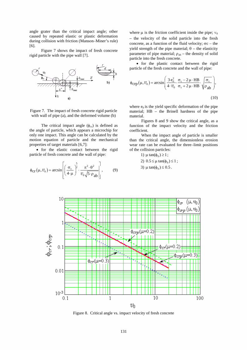
131
angle grater than the critical impact angle; othercaused by repeated elastic or plastic deformationduring collision with friction (Manson–Miner’s rule)[6].
Figure 7 shows the impact of fresh concreterigid particle with the pipe wall [7].
Figure 7. The impact of fresh concrete rigid particlewith wall of pipe (a), and the deformed volume (b)
The critical impact angle (cr) is defined asthe angle of particle, which appears a microchip foronly one impact. This angle can be calculated by themotion equation of particle and the mechanicalproperties of target materials [6,7]:
for the elastic contact between the rigidparticle of fresh concrete and the wall of pipe:
5
2 22c
00
, arcsincr 4 5 ab
vv
, (9)
where is the friction coefficient inside the pipe; v0
– the velocity of the solid particle into the freshconcrete, as a function of the fluid velocity; c – theyield strength of the pipe material; – the elasticityparameter of pipe material; ab – the density of solidparticle into the fresh concrete.
for the plastic contact between the rigidparticle of the fresh concrete and the wall of pipe:
20 c c
00 c
3 e 2 HB, arcsincrp 4 2 HB ab
v v ,
(10)
where e0 is the yield specific deformation of the pipematerial; HB – the Brinell hardness of the pipematerial.
Figures 8 and 9 show the critical angle, as afunction of the impact velocity and the frictioncoefficient.
When the impact angle of particle is smallerthan the critical angle, the dimensionless erosionwear rate can be evaluated for three–limit positionsof the collision particles:
1) 0tan( ) 1 ;
2) 00.5 tan( ) 1 ;
3) 0tan( ) 0.5 .
Figure 8. Critical angle vs. impact velocity of fresh concrete

132
Figure 9. Critical angle vs. friction coefficient of fresh concrete in pipe
The dimensionless erosion rate expression isas follows [8]. For the cases of fresh concrete flow,the erosion rate has the following equations:
the elastic contact:
t
mere 0 0
ab c
t 5
522ab 0 0
e 0 0
8 4I , , r, , t
3
5 sin
4
H , , r, , t ,
v
v
v
(11)
where t is the fatigue parameter of the pipe material,m – the density of pipe material and He – theintegral function which has three forms for the limitcondition of the collision of the fresh concreteparticles;
the plastic contact
t
c
cmerp 0 0
ab
t 5
51 2
0 0abc
p 0 0
2 HB
2 HB8I , , r, , t
3 0.5
1 2 sin
3
H , , r, , t .
v
v
v
(12)
The integral functions He or Hp can beevaluated by numerical methods. A comparisonbetween dimensionless erosion rate for all impactangles of the solid spherical fresh concrete particlein transition to horizontal to vertical pipe is given inFigures 10 and 11 in elastic and plastic deformation.
Figure 10. Pipe erosion rate in elastic contact of solid fresh concrete particle vs. impact angle

133
Figure 11. Pipe erosion rate in plastic contact of solid particle fresh concrete vs. impact angle
Figure 12. Pipe erosion rate in elastic contact of solid particle fresh concrete vs. velocity
Figure 13. Pipe erosion rate in plastic contact of solid particle fresh concrete vs. velocity

134
Figure 14. Pipe erosion rate in elastic contact of solid particle fresh concrete vs. friction coefficient
Figure 15. Pipe erosion rate in plastic contact of solid particle fresh concrete vs. friction coefficient
The maximum erosion rate is a function ofimpact angle of fresh concrete with the verticaldirection of pipe, function of friction with the walland function of velocity of fresh concrete in pipe.
The Figures 12–15 show the effect ofvelocity and friction coefficient on the erosion ratein elastic and plastic deformation of pipes.
5. CONCLUSIONS
The concrete flow through a circular, curvedpipe is different from a circular, straight–lined one.
Thus, the fresh concrete has an axial displacementand angular speed and moves as a „plug”.
The dimensionless contact pressure of freshconcrete increases drastically with the angle of thehorizontal pipe in the vertical direction.
The solid particle of fresh concrete actsabrasive and deforms the pipe material. This effectcan be used to predict the erosion wear rate in elasticor plastic deformation.
The position of maximum erosive wear ratein the curved pipe is a function of friction and offresh concrete velocity.

135
REFERENCES
1. Balayssac, J.P., Detriche, CH., Grandet, J.,1993 “Interet de l’essai d’absorbtion d’eau pour lacaracterisation du beton d’enrobage,” Materials andstructures, 26.2. Tattersall, G.H., 1983, The Rheology of FreshConcrete, Pitman Publish INC, 1983.3. Thomas, N.L. ,Double, D.D., 1981, “Calciumand Silicon Concentrations in Solution During theEarly Hydration of Portland Cement and TricalciumSi,” Cement and Concrete Research, 11, pp. 675 687.4. Vlase, M., Tudor, A., 2009, Pumping andTransport of Concrete Through Pipes (inRomanian), Ed. BREN, Bucureşti.
5. Finnie, I., McFadden, D.H., 1978, On theVelocity Dependence of the Erosion of DuctileMetals by Solid Particles at Low Angles ofIncidence, Wear 48, pp.181–190.6. Kraghelskii, I.V., Dobicin, M.N., Kombalov,V.S., 1977, Osnovi rascetov na trenie i iznos,Moskva, Maşinostroenie.7. Tudor, A., 2002, Frecarea şi uzareamaterialelor, Editura Bren, Bucuresti, 2002.8. Tudor, A., 2003, “An Erosion–Corrosion WearModel for the Ball Valve Crude PetroleumExtraction Pump,” Proceeding Nat. Trib. Conf.,“ROTRIB 03”, 24–26 sept, Galati.

136
(continued from outside back cover)
65 S. LE FLOC’H, M.C. CORNECI, A.-M. TRUNFIO-SFARGHIU, M.-H.MEURISSE, J.-P. RIEU, J. DUHAMEL, C. DAYOT, F. DANG, M. BOUVIER,C. GODEAU, A. SAULOT, Y. BERTHIERImagerie Medicale pour Evaluer les Conditions du FonctionnementTribologiques des Articulations Synoviales
77 M.C. CORNECI, A.-M. TRUNFIO-SFARGHIU, F. DEKKICHE,Y. BERTHIER, M.-H. MEURISSE, J.-P. RIEU, M. LAGARDE,M. GUICHARDANTPhospholipides dans le Fluid Synovial - Influence sur le FonctionnementTribologique des Articulations Synoviales Pathologiques
85 I.C. ROMANU, E. DIACONESCUBioarticular Friction
89 A.-M. TRUNFIO-SFARGHIU, M.C. CORNECI, Y. BERTHIER,M.-H. MEURISSE, J.-P. RIEUMechanical and Physicochemical Analysis of the Tribological Operation ofJoint Replacements
106 D. N. OLARU, C. STAMATE, A. DUMITRASCU, G. PRISACARURolling Friction Torque in Microsystems
113 L. DELEANU, S. CIORTANEvaluating Tribological Damages by 3D Profilometry
120 M. RÎPĂ, S. BOICIUC Characterisation of Laser Cladding with Ni–Cr–B–Fe–Al Alloy byProfilometric Study of the Scratch Tracks
128 M. VLASE, A. TUDORAn Analytical Wear Model of the Pipes for Concrete Transportation


ACTA TRIBOLOGICA VOLUME 18, 2010
CONTENTS
1 A. URZICĂ, S. CRETU A Numerical Procedure to Generate Non-Gaussian Rough Surfaces
7 C. CIORNEI, E. DIACONESCUPreliminary Theoretical Solution for Electric Contact Resistance betweenRough Surfaces
12 C.-I. BARBINTA, S. CRETUThe Influence of the Rail Inclination and Lateral Shift on Pressure Distributionin Wheel - Rail Contact
19 C. SUCIU, E. DIACONESCUPreliminary Theoretical Results upon Contact Pressure Assessment by Aid ofReflectivity
27 S. SPINUNumerical Simulation of Elastic-Plastic Contact
34 Y. NAGATA, R. GLOVNEADielectric Properties of Grease Lubricants
42 J. PADGURSKAS, R. KREIVAITIS, A. KUPČINSKAS, R. RUKUIŽA, V. JANKAUSKAS, I. PROSYČEVAS Influence of Nanoparticles on Lubricity of Base Mineral Oil
46 A.V. RADULESCU, I. RADULESCUInfluence of the Rheometer Geometry on the Rheological Properties ofIndustrial Lubricants
52 V.-F. ZEGREAN, E. DIACONESCUMeasurement of Lubricant Oil Microviscosity Based on Resonant FrequencyShift of AFM Cantilever
58 M.C. CORNECI, A.-M. TRUNFIO-SFARGHIU, F. DEKKICHE, Y.BERTHIER, M.-H. MEURISSE, J.-P. RIEUInfluence of Lubricant Physicochemical Properties on the TribologicalOperation of Fluid Phase Phospholipid Biomimetic Surfaces
(continued on page 136)


