SANDIA REPORT SAND2001-0757 Unlimited Release Printed March 2001 Active Control of Magnetically Levitated Bearings Patrick S. Barney, James P. Lauffer, James M. Redmond, William N. Sullivan Prepared by Sandia National Laboratories Albuquerque, New Mexico 87185 and Livermore, California 94550 Sandia is a multiprogram laboratory operated by Sandia Corporation, a Lockheed Martin Company, for the United States Department of Energy under Contract DE-AC04-94AL85000. Approved for public release; further dissemination unlimited.
Transcript
SANDIA REPORTSAND2001-0757Unlimited ReleasePrinted March 2001
Active Control of Magnetically LevitatedBearings
Patrick S. Barney, James P. Lauffer, James M. Redmond, William N. Sullivan
Prepared bySandia National LaboratoriesAlbuquerque, New Mexico 87185 and Livermore, California 94550
Sandia is a multiprogram laboratory operated by Sandia Corporation,a Lockheed Martin Company, for the United States Department ofEnergy under Contract DE-AC04-94AL85000.
Approved for public release; further dissemination unlimited.
Issued by Sandia National Laboratories, operated for the United States Departmentof Energy by Sandia Corporation.
NOTICE: This report was prepared as an account of work sponsored by an agencyof the United States Government. Neither the United States Government, nor anyagency thereof, nor any of their employees, nor any of their contractors,subcontractors, or their employees, make any warranty, express or implied, orassume any legal liability or responsibility for the accuracy, completeness, orusefulness of any information, apparatus, product, or process disclosed, or representthat its use would not infringe privately owned rights. Reference herein to anyspecific commercial product, process, or service by trade name, trademark,manufacturer, or otherwise, does not necessarily constitute or imply its endorsement,recommendation, or favoring by the United States Government, any agency thereof,or any of their contractors or subcontractors. The views and opinions expressedherein do not necessarily state or reflect those of the United States Government, anyagency thereof, or any of their contractors.
Printed in the United States of America. This report has been reproduced directlyfrom the best available copy.
Available to DOE and DOE contractors fromU.S. Department of EnergyOffice of Scientific and Technical InformationP.O. Box 62Oak Ridge, TN 37831
Active Control of Magnetically Levitated BearingsPatrick S. Barney
Control Subsystems Department
James P. LaufferEngineering Mechanics Modeling and Simulation
James M. RedmondStructural Dynamic Development and Smart Structures
William N. SullivanManufacturing Science and Technology
Sandia National LaboratoriesPO Box 5800
Albuquerque, NM 87185-0501
AbstractThis report summarizes experimental and test results from a two year LDRD projectentitled Real Time Error Correction Using Electromagnetic Bearing Spindles. Thisproject was designed to explore various control schemes for levitating magnetic bearingswith the goal of obtaining high precision location of the spindle and exceptionally highrotational speeds. As part of this work, several adaptive control schemes were devised,analyzed, and implemented on an experimental magnetic bearing system. Measuredresults, which indicated precision positional control of the spindle was possible, agreedreasonably well with simulations. Testing also indicated that the magnetic bearingsystems were capable of very high rotational speeds but were still not immune totraditional structural dynamic limitations caused by spindle flexibility effects.
There were three separate papers written on various advanced schemes for levitating thebearing. Two of these papers presented at the International Modal Analysis Conference(IMAC) in February 2000, and the ASME International Mechanical EngineeringCongress and Exposition in November 2000) are included in this report as appendices.
Acknowledgements
The authors would like to thank Brad Paden (Magnetic Moments, Inc) who shared muchof his valuable experience with magnetic bearing systems and developed the MBC 500that was used extensively in this project. Professor Gordon Parker and his studentRebecca Petteys of Michigan Technical University contributed significantly to thetheoretical and experimental work presented in this report.
Introduction and Results
Supporting rotating spindles with magnetic bearings offers a number of advantages overconventional fluid or ball/roller bearings. Magnetic bearings generally have very lowdrag, do not require any lubrication, and there is no physical contact between the spindleand the bearing. These characteristics make these bearings very useful for applicationswhere low friction, high speed, cleanliness, and maintenance free life are needed. Anumber of systems (precision gyroscopes and artificial heart pumps are examples) havebeen built utilizing these advantages.
Magnetic bearings have some disadvantages as well. They are usually unstable andrequire active control systems to ensure the spindle is properly levitated within thejournal. Their stiffness is relatively low, compared to conventional bearings. They aremore expensive and bulkier than conventional bearings, mainly due to the size ofmagnets needed and the supporting equipment required.
This LDRD project started out with the goal of looking at improved control algorithmsthat could levitate a magnetic bearing more precisely and adjust for changing loadconditions on the spindle. This sort of control was envisioned as enabling magneticbearings to be more suitable for high speed or micro machining applications, where highRPM and very precise control of the spindle location are necessary. To evaluatealternative control schemes and explore the high RPM capabilities, a laboratory scalemagnetic bearing demonstrator (MBC 500) was procured from Magnetic Moments, Inc.This system came with its own internal controls that levitated the bearing. In addition,the setup allowed insertion of alternative controllers either in parallel or in replacement ofthe built-in controller. This proved to be a very useful setup for evaluating a variety ofcontrol algorithms. Several modifications were made to the spindle and its air turbinedrive to explore the high RPM performance envelope.
Two adaptive control schemes were implemented and evaluated. The first, an adaptiveLMS (Least Mean Squares) controller was created with a programmable digital signalprocessing (DSP) card and installed in parallel to the built-in controller. This controllerwas able to effectively center a wobble in the system due to shaft imbalance. The resultsof this work are summarized in Appendix A. The second controller used an APACA(Amplitude-Phase Adaptive Control Algorithm) approach. This controller wasimplemented similarly to the LMS algorithm, and the results summarized Appendix B.
Both adaptive algorithms were mathematically modeled using a commercial, generalpurpose simulation tool (Simulink® ) and the results were compared with measurementson the MBC 500 demonstrator. The agreement between test and experiment was quitegood, and both adaptive controllers offered significant improvement in spindleconcentricity in the bearing relative to the built-in, non-adaptive controller.
A limited number of tests were conducted with the LMS algorithm to determine themaximum speed capability of the MBC 500 bearing demonstrator. The first series oftests showed that the LMS algorithm adapted well to reduce eccentricity due to
imbalance, but the algorithm was still incapable of stabilizing the shaft through its firstcritical frequency at 40,000 RPM. Although efforts were made to balance the shaft moreprecisely and to modify the drive turbine to accelerate the shaft more rapidly through thefirst critical speed, this still did not allow speeds above 40,000 RPM.
Magnetic Moments eventually modified our MBC 500 with a much shorter shaft thatwould have a correspondingly higher first bending mode and critical speed. MaximumRPM with this system operating with the LMS algorithm was approximately 120,000RPM.
Conclusions
The experiments and analysis of controllers indicate that magnetic bearing systems arewell suited for control using modern automatic control algorithms. The adaptivealgorithms investigated are capable of producing stable bearing performance whilereducing eccentricity errors due to applied loads. They are relatively easy to implementwith today’s programmable digital signal processing capabilities.
Magnetic bearings are indeed capable of very high rotational speeds, and we successfullydrove our spindle to 120,000 RPM. However, the controllability of the bearing did notallow the spindle to overcome traditional structural dynamic limitations on spindle speedscaused by vibrational modes in the spindle.
APPENDIX A
Active Control of a Magnetically Levitated Spindle
Partick Barney, James Lauffer, James Redmond, William SullivanSandia National Laboratories.
Presented at the International Modal Analysis ConferenceFebruary 2000San Antonio, TX
ACTIVE CONTROL OF A MAGNETICALLY LEVITATED SPINDLE *
Patrick Barney1 , James Lauffer1, James Redmond2, William Sullivan3
Sandia National LaboratoriesAlbuquerque, NM 87185
1Experimental Structural Dynamics Department MS 05572Structural Dynamics and Vibration Control Department MS 0847
3Mechanical Engineering Department MS 0958
* Sandia National Laboratories is a multiprogram laboratory operated by Sandia Corporation, a Lockheed Martin Company, for the United
States Department of Energy under Contract DE-AC04-94AL85000.
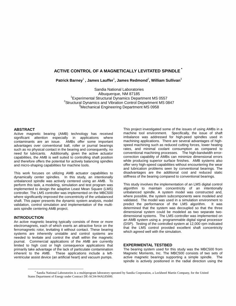
ABSTRACTActive magnetic bearing (AMB) technology has receivedsignificant attention especially in applications wherecontaminants are an issue. AMBs offer some importantadvantages over conventional ball, roller or journal bearingssuch as no physical contact in the bearing and consequently, noneed for lubricants. Additionally, given the active actuatorcapabilities, the AMB is well suited to controlling shaft positionand therefore offers the potential for actively balancing spindlesand micro-shaping capabilities for machine tools.
This work focuses on utilizing AMB actuator capabilities todynamically center spindles. In this study, an intentionallyunbalanced spindle was actively centered using an AMB. Toperform this task, a modeling, simulation and test program wasimplemented to design the adaptive Least Mean Square (LMS)controller. The LMS controller was implemented on the MBC500where significantly improved the concentricity of the unbalancedshaft. This paper presents the dynamic system analysis, modelvalidation, control simulation and implementation of the multi-axis spindle centering AMB project.
INTRODUCTIONAn active magnetic bearing typically consists of three or moreelectromagnets, each of which exerts an attractive force on theferromagnetic rotor, levitating it without contact. These bearingsystems are inherently unstable and control systems areneeded to levitate and control the shaft within the magneticjournal. Commercial applications of the AMB are currentlylimited to high cost or high consequence applications thatprimarily take advantage of the lack of particulate contaminationinherent to the AMB. These applications include a left-ventricular assist device (an artificial heart) and vacuum pumps.
This project investigated some of the issues of using AMBs in amachine tool environment. Specifically, the issue of shaftimbalance was addressed for high-peed spindles used inmachining applications. There are several advantages of high-speed machining such as reduced cutting forces, lower heatingrates, and minimal coolant consumption as compared toconventional machining processes. The high-bandwidth error-correction capability of AMBs can minimize dimensional errorswhile producing superior surface finishes. AMB systems alsooffer very high-speed capabilities without encountering the wearand lubrication problems seen by conventional bearings. Thedisadvantages are the additional cost and reduced staticstiffness of the bearing compared to conventional bearings.
This study involves the implementation of an LMS digital controlalgorithm to maintain concentricity of an intentionallyunbalanced spindle. A system model was constructed and,where possible, the system subcomponents were modeled andvalidated. The model was used in a simulation environment topredict the performance of the LMS algorithm. It wasdetermined that the system was decoupled so that the threedimensional system could be modeled as two separate two-dimensional systems. The LMS controller was implemented onan AMB system using a programmable digital signal processor(DSP). Testing of the controlled system at 12,000 rpm indicatedthat the LMS control provided excellent shaft concentricitywhich agreed well with the simulation.
EXPERIMENTAL TESTBEDThe bearing system used for this study was the MBC500 fromMagnetic Moments, Inc. The MBC500 consists of two sets ofactive magnetic bearings supporting a simple spindle. Thespindle is actively positioned in the radial direction using the
integrated analog sensor and control system. The shaft rotatesabout its longitudinal axis and is driven by an air turbine tospeeds above 40,000 RPM. To provide a completely self-contained system, the controllers, sensors, actuators andconditioners were all integrated into the MBC500[1]. The systemaccommodated teeing into the sensors and actuators as well asbypassing the internal controllers which made the MBC500 anexcellent choice for AMB control design.
SIMULATION MODELThe AMB system was modeled using a general purposesimulation environment (Simulink ). The need for a time-marching non-linear simulation environment was due to thenon-linearities in the electromagnets and sensors. The purposeof the simulation was to aid in predicting the performance of theLMS. The system block diagram model of the MBC500 isshown in Figure 1.
f(u)
Sensor
x' = Ax+Bu y = Cx+Du
Plant Dynamics
Disp
CurrentForce
Motor/Amp
PID VdispIcont
Input Force Displacement 'X'
Controller
External Force
Figure 1 – System block diagram
As seen in the block diagram the major system componentsinclude the plant (the simple spindle dynamics), the sensor(eddy current), the internal analog controller (Proportional-Integral-Derivative) and the actuator (AMB). The followingsections describe the modeling of each of the systemsubcomponents.
Plant DynamicsIn the system model shown in Figure 1, plant dynamics consistof the free-free modes of the shaft. Since the gyroscopicaffects are negligible, and the system is symmetric(mechanically and electrically), the model was reduced to atwo-dimensional system. Although the system never goesthrough a critical speed for these tests, it is important to modelthe spindle flexible-body dynamics to obtain good controlsimulation fidelity. In this case, the first bending modes of thetwo dimensional shaft were included in this simulation. Asimple Finite Element Analysis (FEA) was performed usingfree-free conditions to obtain the dynamic equations. The firsttwo bending modes for the spindle are shown in Figure 3 alongwith the AMB force input locations.
F1 F2
Mode 1
Mode 2
Figure 2 – First two bending modes of the spindle.
The analytically derived mass and stiffness matrices wereaugmented with an experimentally derived damping matrix.Using the rigid-body and flexible-body equations the plant state-space model was assembled as shown in Equation 1 below.
PPP
PPPPP
XCY
FBXAX
=+=�
(1)
where ‘P’ signifies the plant matrices and states. In this model,the restoring forces of the plant (shaft) are those exerted by themagnets, which are not included in the state-space model.These AMB forces are used as the inputs (F) to the state-spacemodel, while the outputs (Y) of the system are the positions ofthe shaft.
Sensor DynamicsThe control feedback sensors for this AMB system consist oftwo orthogonal eddy current proximity probes at each shaft endnear the AMB center of force (nearly colocated). The target forthe eddy current sensors is the circular shaft that inherentlymakes the output of voltage versus displacement somewhat non-linear in the operating region. The output voltage with respectto meters displacement is given as
3910245000 iisense XXVi
×+= (2)
Figure 3 provides the displacement versus voltage for a givenaxis. As can be seen by the plot, the output is relatively linearfor small deflections but the non-linearity becomes morepronounced at the higher displacement levels (hardening springeffect). The range of motion for the MBC500 shaft is .0004meters; Figure 3 is shown with a range to .0003 meters to de-emphasize the stronger non-linear affects with displacementsabove .0003 meters.
0 0.5 1 1.5 2 2.5 3x 10⁻⁴
0
0.5
1
1.5
2
2.5
Displacement (meters)
Sensor output )
Volts
Figure 3 – Eddy current sensor voltage output vs.displacement
Controller DynamicsThere are four independent PID analog controllers supplied withthe MBC500. Each controller uses a single axis sensor voltageas input and produces an output voltage that controls the
magnetic force (a pair of pull-pull magnets) for that particularaxis. The transfer function for the controller is
sensecontrol Vss
sV
����
�
×+×+×+= −−
−
)102.21)(103.31()109.81(41.1
54
4
(3)
The implementation is primarily proportional feedback of thesensor displacement. For a truly colocated sensor-actuator pairand a linear uncoupled system, this is a very robust controller,and for this application it works very well. In essence, theproportional displacement feedback offers a virtual stiffness tothe system that results in a bounce mode at about 70 hertz anda pitch mode at about 45 hertz. The non-linearity in the system(mostly due to the actuator) adds effective damping to thesystem and the result is a well behaved mechanical system.
Active Magnetic Motor DynamicsThe magnets can only exert an attractive force so each bearingconsists of four electromagnets. These electromagnets arepositioned in a simple opposing pull-pull arrangement for eachorthogonal axis at each end of the spindle. A simple cartoondiagram of a single electromagnet is shown in Figure 4.
I
N
A
gFigure 4 – Simple electromagnet, ferous target and
resultant forces.
The force exerted by one electromagnet on the shaft is
2
220
4g
INAF
µ= (4)
where A is the cross-sectional area of the magnet, µ0 is thepermittivity of free space, g is the gap between theelectromagnet and the rotor, and N is the number of coils in themagnet, each carrying current I. The MBC500 has a gap of0.0004 meters and a bias current of 0.5 amperes at equilibrium.The total force on the shaft at one bearing due to both magnets(in one axis) is
2
2
2
2
)0004.0()5.0(
)0004.0()5.0(
−+−
+−=
x
Ik
x
IkF (5)
where k = Aµ0N2/4.
As can be seen by the equation above, the output force of theAMB is highly non-linear with respect to the inputs; the force isproportional to the square of the controller current, and is
inversely proportional to the square of the gap. Figure 5provides an output force map from the actuator as a function ofcontrol voltage and shaft displacement. As can be seen by thisfigure, the output forces become highly non-linear as both thedisplacement and control voltage become large.
Figure 5 – AMB force output as a function of bearinggap and control voltage.
Modeling the closed loop systemAs discussed earlier, a full simulation of the AMB system isnecessary because of the non-linearities in the system. Strongsystem non-linearities do not allow for accurate linear analysiswhen trying to predict the response of a system especially whenit is to be used for closed-loop control-algorithm development.Because of this, a time marching simulation method must beemployed to offer reasonable prediction accuracy. Additionally,the operating amplitudes of the simulation must be close tothose expected in service (or in the validation experiments) orthe resulting predictions may have significant errors. The basicmodel was first exercised using Simulink to produce modelvalidation data as presented in the following sections. Next, themodel was used to determine the effectiveness of an LMSalgorithm for mitigating shaft eccentricity.
System ValidationThe validation of a system model for predictive simulationtypically requires a great effort. The first step in the process isto determine how success will be qualified in terms of the goalof the prediction and the significance of the error sources. Inthis case, the purpose of the simulation was to evaluatealternative control approaches to the imbalance problem of anAMB shaft. Particularly, the LMS algorithm was being evaluatedfor its performance in a steady state mode of operation.
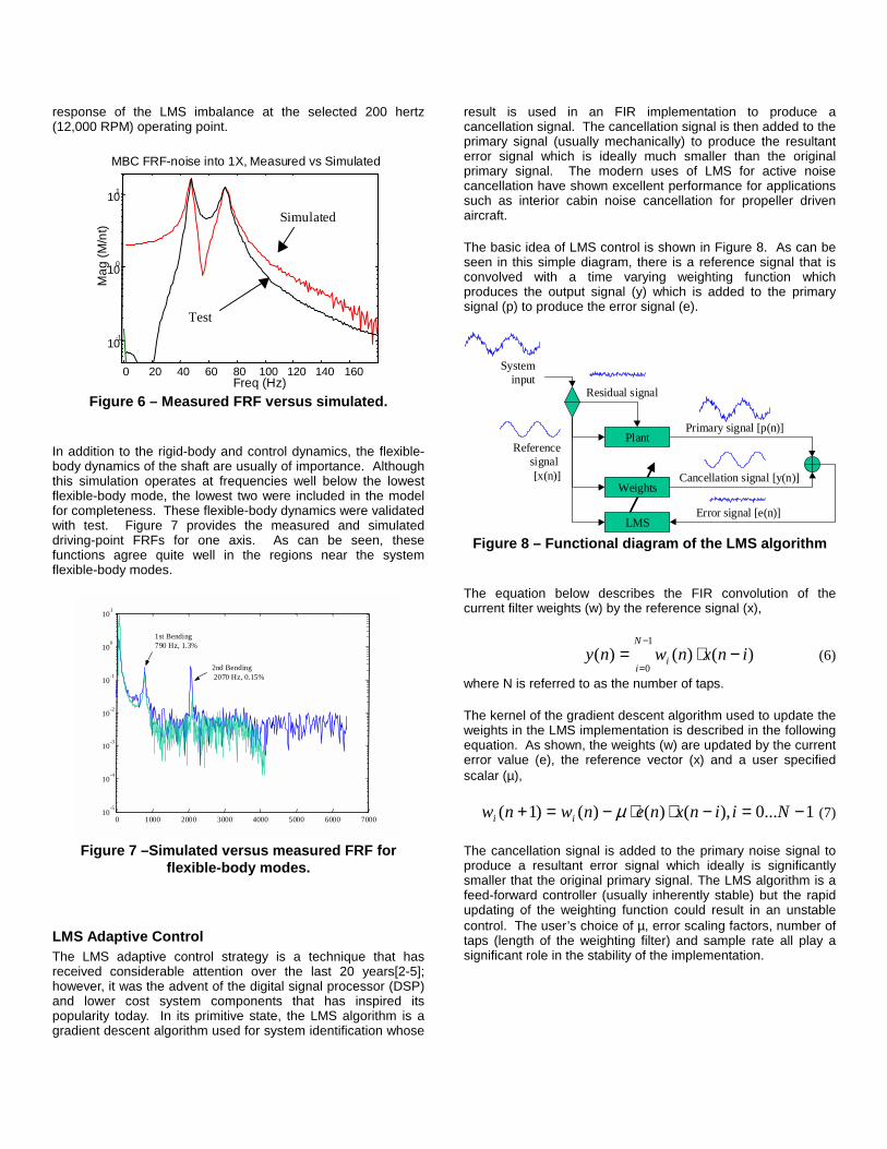
To perform this task, it was assumed that a good representationof the rigid-body modes of the system was important. Therepresentation selected for this comparison task was thesystem FRF from AMB actuator forces to the sensor deflectionsnear a nominal operating amplitude. Figure 6 provides thesimulated and measured FRFs for input at one actuator and itsrespective response. As can be seen, the model compares wellat the resonance. The deviation of the FRF off resonance(especially at the low frequencies) will not particularly affect the
response of the LMS imbalance at the selected 200 hertz(12,000 RPM) operating point.
0 20 40 60 80 100 120 140 160
10-1
100
101
MBC FRF-noise into 1X, Measured vs Simulated
Mag
(M/n
t)
Freq (Hz)
Simulated
Test
Figure 6 – Measured FRF versus simulated.
In addition to the rigid-body and control dynamics, the flexible-body dynamics of the shaft are usually of importance. Althoughthis simulation operates at frequencies well below the lowestflexible-body mode, the lowest two were included in the modelfor completeness. These flexible-body dynamics were validatedwith test. Figure 7 provides the measured and simulateddriving-point FRFs for one axis. As can be seen, thesefunctions agree quite well in the regions near the systemflexible-body modes.
0 1000 2000 3000 4000 5000 6000 700010
-5
10-4
10-3
10-2
10-1
100
101
1st Bending 790 Hz, 1.3%
2nd Bending 2070 Hz, 0.15%
Figure 7 –Simulated versus measured FRF forflexible-body modes.
LMS Adaptive ControlThe LMS adaptive control strategy is a technique that hasreceived considerable attention over the last 20 years[2-5];however, it was the advent of the digital signal processor (DSP)and lower cost system components that has inspired itspopularity today. In its primitive state, the LMS algorithm is agradient descent algorithm used for system identification whose
result is used in an FIR implementation to produce acancellation signal. The cancellation signal is then added to theprimary signal (usually mechanically) to produce the resultanterror signal which is ideally much smaller than the originalprimary signal. The modern uses of LMS for active noisecancellation have shown excellent performance for applicationssuch as interior cabin noise cancellation for propeller drivenaircraft.
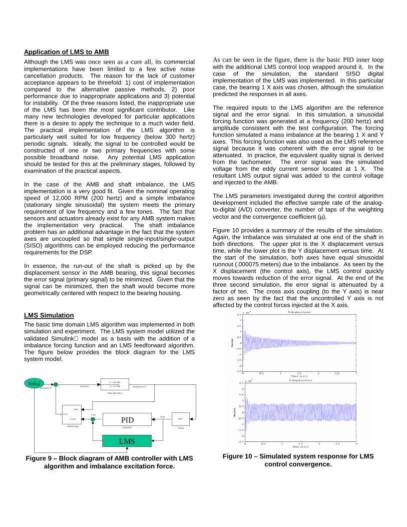
The basic idea of LMS control is shown in Figure 8. As can beseen in this simple diagram, there is a reference signal that isconvolved with a time varying weighting function whichproduces the output signal (y) which is added to the primarysignal (p) to produce the error signal (e).
Plant
Weights
LMS
Systeminput
Referencesignal [x(n)]
Primary signal [p(n)]
Cancellation signal [y(n)]
Error signal [e(n)]
Residual signal
Figure 8 – Functional diagram of the LMS algorithm
The equation below describes the FIR convolution of thecurrent filter weights (w) by the reference signal (x),
)()()(1
0inxnwny i
N
i−⋅=
−
= (6)
where N is referred to as the number of taps.
The kernel of the gradient descent algorithm used to update theweights in the LMS implementation is described in the followingequation. As shown, the weights (w) are updated by the currenterror value (e), the reference vector (x) and a user specifiedscalar (µ),
1...0),()()()1( −=−⋅⋅−=+ Niinxnenwnw ii µ (7)
The cancellation signal is added to the primary noise signal toproduce a resultant error signal which ideally is significantlysmaller that the original primary signal. The LMS algorithm is afeed-forward controller (usually inherently stable) but the rapidupdating of the weighting function could result in an unstablecontrol. The user’s choice of µ, error scaling factors, number oftaps (length of the weighting filter) and sample rate all play asignificant role in the stability of the implementation.
Application of LMS to AMBAlthough the LMS was once seen as a cure all, its commercialimplementations have been limited to a few active noisecancellation products. The reason for the lack of customeracceptance appears to be threefold: 1) cost of implementationcompared to the alternative passive methods, 2) poorperformance due to inappropriate applications and 3) potentialfor instability. Of the three reasons listed, the inappropriate useof the LMS has been the most significant contributor. Likemany new technologies developed for particular applicationsthere is a desire to apply the technique to a much wider field.The practical implementation of the LMS algorithm isparticularly well suited for low frequency (below 300 hertz)periodic signals. Ideally, the signal to be controlled would beconstructed of one or two primary frequencies with somepossible broadband noise. Any potential LMS applicationshould be tested for this at the preliminary stages, followed byexamination of the practical aspects.
In the case of the AMB and shaft imbalance, the LMSimplementation is a very good fit. Given the nominal operatingspeed of 12,000 RPM (200 hertz) and a simple imbalance(stationary single sinusoidal) the system meets the primaryrequirement of low frequency and a few tones. The fact thatsensors and actuators already exist for any AMB system makesthe implementation very practical. The shaft imbalanceproblem has an additional advantage in the fact that the systemaxes are uncoupled so that simple single-input/single-output(SISO) algorithms can be employed reducing the performancerequirements for the DSP.
In essence, the run-out of the shaft is picked up by thedisplacement sensor in the AMB bearing, this signal becomesthe error signal (primary signal) to be minimized. Given that thesignal can be minimized, then the shaft would become moregeometrically centered with respect to the bearing housing.
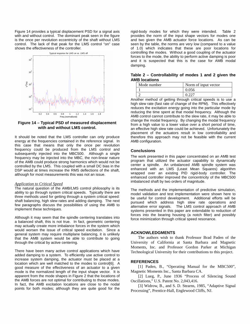
LMS SimulationThe basic time domain LMS algorithm was implemented in bothsimulation and experiment. The LMS system model utilized thevalidated Simulink model as a basis with the addition of aimbalance forcing function and an LMS feedforward algorithm.The figure below provides the block diagram for the LMSsystem model.
f(u)
Sensor
x' = Ax+Bu
y = Cx+Du
Plant Dynamics
Disp
Current
Force
Motor /Amp
PIDVdisp
Vcont
Input Force Displacement 'X'
Controlle r
External Force
LMS
Imbal
Figure 9 – Block diagram of AMB controller with LMSalgorithm and imbalance excitation force.
As can be seen in the figure, there is the basic PID inner loopwith the additional LMS control loop wrapped around it. In thecase of the simulation, the standard SISO digitalimplementation of the LMS was implemented. In this particularcase, the bearing 1 X axis was chosen, although the simulationpredicted the responses in all axes.
The required inputs to the LMS algorithm are the referencesignal and the error signal. In this simulation, a sinusoidalforcing function was generated at a frequency (200 hertz) andamplitude consistent with the test configuration. The forcingfunction simulated a mass imbalance at the bearing 1 X and Yaxes. This forcing function was also used as the LMS referencesignal because it was coherent with the error signal to beattenuated. In practice, the equivalent quality signal is derivedfrom the tachometer. The error signal was the simulatedvoltage from the eddy current sensor located at 1 X. Theresultant LMS output signal was added to the control voltageand injected to the AMB.
The LMS parameters investigated during the control algorithmdevelopment included the effective sample rate of the analog-to-digital (A/D) converter, the number of taps of the weightingvector and the convergence coefficient (µ).
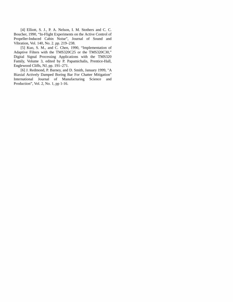
Figure 10 provides a summary of the results of the simulation.Again, the imbalance was simulated at one end of the shaft inboth directions. The upper plot is the X displacement versustime, while the lower plot is the Y displacement versus time. Atthe start of the simulation, both axes have equal sinusoidalrunnout (.000075 meters) due to the imbalance. As seen by theX displacement (the control axis), the LMS control quicklymoves towards reduction of the error signal. At the end of thethree second simulation, the error signal is attenuated by afactor of ten. The cross axis coupling (to the Y axis) is nearzero as seen by the fact that the uncontrolled Y axis is notaffected by the control forces injected at the X axis.
0 0.5 1 1.5 2 2.5 3-2.5
-2
-1.5
-1
-0.5
0
0.5
1
1.5
2
2.5x 10
-4
Disp
(m)
Y d isp la cem en t
Time (s ec )
0 0.5 1 1.5 2 2.5 3- 2.5
-2
- 1.5
-1
- 0.5
0
0.5
1
1.5
2
2.5x 10
-4 X dis pla ce m en t
Disp
(m)
Tim e (s ec )
Figure 10 – Simulated system response for LMScontrol convergence.
LMS ExperimentThe basic time domain LMS algorithm was implemented inexperiment using the MBC500 and the LMS simulationapproach. The natural imbalance of the shaft was sufficient forreasonable eccentric rotation at 12,000 RPM. The once perrevolution tachometer provided a very clean signal which wascoherent with the imbalance as required for LMS.
The PC-based DSP system was programmed for a SISO LMSwith the capability to update µ in real-time. The nominalparameters from simulation were used in the baseline DSPimplementation and are given in Table 1
sample frequency 2000 HzFilter length (w) 20 tapsµ VariableReference Tachometer
As shown in the table, µ was selected as variable to account forscaling issues within the A/D of the DSP.
Figure 11 provides a summary of the results of the test. Theupper plot is the X displacement (volts) versus time, while thelower plot is the Y displacement (volts) versus time. At the startof the simulation, both axes have equal sinusoidal run-out(.000075 meters) due to the imbalance. As seen by the Xdisplacement (the control axis), the LMS control quicklyattenuates the error signal (orders of magnitude). The crossaxis coupling (to the Y axis) is near zero as seen by the fact thatthe uncontrolled Y axis is not affected by the control forcesinjected at the X axis.
0 2 4 6 8 10 12 14 16-1
0
1
X D
isp
0 2 4 6 8 10 12 14 16-0.5
0
0.5
Y D
isp
Time (sec)
Control off
Control on
Figure 11 –LMS implementation on AMB shaftimbalance (control on versus control off).
Compared to the simulation, the results of this test are verygood and converge even more quickly. The reason for thequicker convergence is that the µ used in the test was higherthan that of the simulation. Although the attenuation of theimbalance is fast, the impulsive nature of the control force whenfirst activated causes a rigid-body motion which takes a fewseconds to settle out.
Multi-Axis ExperimentAs stated earlier, it was suspected and confirmed throughmodal experiments that the system axes were reasonablydecoupled. Due to the uncoupled system dynamics, the singleaxis LMS control experiment could be extended to twoindependent control implementations. The single tachometersignal and the displacement error signals were fed intoseparate LMS algorithms which produced independent controlsignals. Figure 12 presents the measured shaft deflections forthe two-axis LMS control off versus LMS on.
0 0.5 1 1.5 2-0.05
0
0.051-X
Vol
ts
0 0.5 1 1.5 2-0.05
0
0.051-Y
0 0.5 1 1.5 2-0.05
0
0.052-X
Vol
ts
Time (sec)
LMS Control Transient: X axis only
0 0.5 1 1.5 2-0.05
0
0.052-Y
Time (sec)
Figure 12 – Measured shaft deflections for the two-axis LMS control.
As can be seen in the figure, at the start there is a significantonce per revolution displacement on all axes due to theimbalance. At 0.3 seconds, the control is turned on for the Xaxes and their displacements are significantly reduced. The Yaxes deflections are also somewhat reduced over time.Figure 13 provides similar results for the four axes LMSimplementation. As can be seen by the plot, all axis havesignificant reduction of the out-of-roundness errors.
0 0.5 1 1.5 2-0.05
0
0.051-X
Vol
ts
0 0.5 1 1.5 2-0.05
0
0.051-Y
0 0.5 1 1.5 2-0.05
0
0.052-X
Vol
ts
Time (sec)
LMS Control Transient: All axis
0 0.5 1 1.5 2-0.05
0
0.052-Y
Time (sec)
Figure 13 – Measured shaft deflections for the four-axis LMS control.
Figure 14 provides a typical displacement PSD for a signal axiswith and without control. The dominant peak seen in the figureis the once per revolution eccentricity of the shaft without LMScontrol. The lack of that peak for the LMS control “on” caseshows the effectiveness of the controller.
0.2 0.4 0.6 0.8 1 1.2 1.4 1.6 1.8
10-1
100
101
102
103
Freq (normallized)
V2 /H
z
Typical response for LMS on vs. LMS off
Figure 14 – Typical PSD of measured displacementwith and without LMS control.
It should be noted that the LMS controller can only produceenergy at the frequencies contained in the reference signal. Inthis case that means that only the once per revolutionfrequency could be produced from the LMS control andsubsequently injected into the MBC500. Although a singlefrequency may be injected into the MBC, the non-linear natureof the AMB could produce strong harmonics which would not becontrolled by the LMS. This coupled with a small DC bias in theDSP would at times increase the RMS deflections of the shaft,although for most measurements this was not an issue.
Application to Critical SpeedThe natural question of the AMB/LMS control philosophy is itsability to go through system critical speeds. Typically there arethree methods used for getting through a system critical speed:shaft balancing, high slew rates and adding damping. The nextfew paragraphs discuss the possibilities of using the AMB toimplement these techniques.
Although it may seem that the spindle centering translates intoa balanced shaft, this is not true. In fact, geometric centeringmay actually create more imbalance forces in the system whichwould worsen the issue of critical speed excitation. Since ageneral system may require multiplane balancing, it is unlikelythat the AMB system would be able to contribute to goingthrough the critical by active centering.
There have been many active control applications which haveadded damping to a system. To efficiently use active control toincrease system damping, the actuator must be placed at alocation which are well matched to the modes to control[6]. Agood measure of the effectiveness of an actuator to a givenmode is the normalized length of the input shape vector. It isapparent from the mode shapes in Figure 2 that the locations ofthe AMB forces are not optimal for contributing to those modes.In fact, the AMB excitation locations are close to the nodalpoints for both modes; although they are quite good for the
rigid-body modes for which they were intended. Table 2provides the norm of the input shape vectors for modes oneand two given the AMB actuator force locations. As can beseen by the table, the norms are very low (compared to a valueof 1.0) which indicates that these are poor locations forcontrolling the modes. Without a good coupling of the actuatorforces to the mode, the ability to perform active damping is poorand it is suspected that this is the case for AMB modaldamping.
Table 2 – Controllability of modes 1 and 2 given theAMB locations
Mode number Norm of input vector1 0.0562 0.227
Another method of getting through critical speeds is to use ahigh slew rate (fast rate of change of the RPM). This effectivelyreduces the excitation energy going into the particular mode byreducing the time spent at that modal frequency. Although theAMB control cannot contribute to the slew rate, it may be able tochange the modal frequency. By changing the modal frequencyfrom a high value to a lower value over a short period of time,an effective high slew rate could be achieved. Unfortunately theplacement of the actuators result in low controllability andtherefore this approach may not be feasible with the currentAMB configuration.
ConclusionsThe work presented in this paper concentrated on an AMB testprogram that utilized the actuator capability to dynamicallycenter a spindle. An unbalanced AMB spindle system wasenhanced with an LMS (Least Mean Squares) algorithmwrapped over an existing PID rigid-body controller. Theenhanced controller improved the concentricity of the MBC500imbalanced shaft by two orders of magnitude.
The methods and the implementation of predictive simulation,model validation and test implementation were shown here tobe useful for control development. Additional efforts will bepursued which address high slew rate operations andalternative error signals. The LMS control approach of AMBsystems presented in this paper are extendable to reduction offorces into the bearing housing (a notch filter) and possiblyforce minimization through critical speed resonance.
ACKNOWLEDGMENTSThe authors wish to thank Professor Brad Paden of the
University of California at Santa Barbara and MagneticMoments, Inc. and Professor Gordon Parker at MichiganTechnological University for their contributions to this project.
REFERENCES[1] Paden, B., “Operating Manual for the MBC500”,
Magnetic Moments Inc., Santa Barbara CA.[2] Lueg, P., June 1936 “Process of Silencing Sound
Oscillations,” U.S. Patent No. 2,043,416.[3] Widrow, B., and S. D. Stearns, 1985, “Adaptive Signal
Processing”, Prentice-Hall, Englewood Cliffs, NJ.
[4] Elliott, S. J., P. A. Nelson, I. M. Stothers and C. C.Boucher, 1990, “In-Flight Experiments on the Active Control ofPropeller-Induced Cabin Noise”, Journal of Sound andVibration, Vol. 140, No. 2. pp. 219–238.
[5] Kuo, S. M., and C. Chen, 1990, “Implementation ofAdaptive Filters with the TMS320C25 or the TMS320C30,”Digital Signal Processing Applications with the TMS320Family, Volume 3, edited by P. Papamichalis, Prentice-Hall,Englewood Cliffs, NJ, pp. 191–271.
[6] J. Redmond, P. Barney, and D. Smith, January 1999, "ABiaxial Actively Damped Boring Bar For Chatter Mitigation"International Journal of Manufacturing Science andProduction”, Vol. 2, No. 1, pp 1-16.
APPENDIX B
Disturbance Rejection Control of an Electromagnetic BearingSpindle
Rebecca Petteys and Gordon ParkerMichigan Technological University
James RedmondSandia National Laboratories.
Presented at the ASME International Mechanical Engineering Congress and ExpositionNovember 2000Orlando, FL"Adaptive Structures and Material Systems," AD-Vol. 60, pp. 461-468.
Disturbance Rejection Control of an Electromagnetic Bearing Spindle
Rebecca PetteysGordon Parker
Michigan Technological UniversityDepartment of Mechanical Engineering
1400 Townsend Dr.Houghton, MI 49931
James RedmondSandia National Laboratories
Albuquerque, NM 87111
ASTRACTThe force exerted on the rotor by an active magnetic bearing isdetermined by the current flow in the magnet coils. This forcecan be controlled very precisely, making magnetic bearings apotential benefit for grinding, where cutting forces act as exter-nal disturbances on the shaft, resulting in degraded part finish. Itis possible to achieve precise shaft positioning, reduce vibrationof the shaft caused by external disturbances, and even damp outresonant modes. Adaptive control is an appealing approach forthese systems because the controller can tune itself to accountfor an unknown periodic disturbance, such as cutting or grindingforces, injected in to the system. In this paper we show how oneadaptive control algorithm can be applied to an AMB systemwith a periodic disturbance applied to the rotor. An adaptivealgorithm was developed and implemented in both simulationand hardware, yielding significant reductions in rotor displace-ment in the presence of an external excitation. Ultimately, thistype of algorithm could be applied to a magnetic bearing grinderto reduce unwanted motion of the spindle which leads to poorpart finish and chatter.
INTRODUCTIONIn magnetic bearing systems, a spindle is levitated with mag-netic fields created by either permanent magnets or electromag-nets (or both) so that no part of the spindle comes in contactwith the bearings. With permanent magnets, the force exertedon the rotor can be either attractive or repulsive. A repulsiveforce results in a system that is stable without a controller. How-ever, the force exerted by the permanent magnets cannot be con-trolled and is limited by the strength of the magnets. Withelectromagnets, the force on the rotor can be varied by changingthe current flow in the magnet coils. This results in an activemagnetic bearing (AMB). However, the levitating forces areattractive, making the system inherently unstable and requiringthe use of a controller.
The force exerted by the electromagnets can be controlledwithin N, making it possible to achieve precise shaft posi-tioning, reduce vibration of the shaft caused by external distur-bances, and even damp out resonant modes. This makesmagnetic bearings a potential benefit for grinding and other
0.05±
metal cutting processes, where cutting forces act as external dis-turbances on the shaft, resulting in degraded part finish. AMBsystems also do not have the wear and lubrication problems seenby conventional bearings, but require additional electronic andcooling systems. Furthermore, they are limited in load capabil-ity
Adaptive control is an appealing approach for these systemsbecause the controller can tune itself to account for an unknownperiodic disturbance, such as cutting forces injected in to thesystem. In this paper we show how one adaptive control algo-rithm can be applied to an AMB system with a periodic distur-bance applied to the rotor. The purpose is to create an inputsignal that would counteract the disturbance and result in mini-mal motion of the spindle. In an application such as grinding,this would result in improved part finish, reduction of chatter,etc. First a model of the experimental system must be developedto test the proposed control strategy. Then the adaptive controlalgorithm will be described and results will be shown.
EXPERIMENTAL SETUPThe bearing system modelled and used for this paper is a modi-fied MBC500 from Magnetic Moments, Inc. The MBC500 hastwo active magnetic bearings, each consisting of four electro-magnets, supporting the spindle. The bearings are mounted ontop of an anodized aluminum case which houses the electronicsand also acts as a heat sink for the magnets. The spindle isactively positioned in the radial direction at the bearings andfreely rotates about its long axis. The front panel shows a blockdiagram of the system with BNC connections for easy access tosystem inputs and outputs. An air turbine drives the shaft tospeeds up to 10,000 RPM.
The system has four on-board analog lead-filter controllers thatlevitate the spindle in its default mode. These controllers can bedisabled with switches on the front panel, allowing an externalcontroller to be implemented. The BNC connections also allowfor an external controller to be wrapped around the on-boardcontrollers while they are still engaged. The modified version ofthe MBC500 include an external electromagnet mounted on thecase near the center of the spindle to be used as a disturbancesource. The magnet can be moved to vary the gap between themagnet and the spindle, thereby allowing for a large range ofapplied forces. The current flow to this magnet is controlled byan external amplifier.
SYSTEM MODELAn accurate model of the system is necessary for designing andtesting prospective control strategies. Magnetic bearings arehighly nonlinear by nature and, in order to best capture theeffects of those nonlinearities, a Simulink simulation wasdesigned. A block diagram representation of the system isshown in Figure 1. This diagram represents the MBC500 with-
out any external controllers, but with the external magnet apply-ing a disturbance force to the spindle. It is assumed that thespindle is not spinning, so there are no gyroscopic effects andthe axes are completely uncoupled. The external force isassumed to be applied exactly at the center of the shaft. The sys-tem inputs and outputs are also shown.
Figure 1. Simulink model used to simulate themagnetic bearing system
When external controllers are implemented, either the feedbackloop containing the lead-filter compensators is broken andreplaced with a computer system which implements the digitalcontrollers, or an external controller is wrapped around the on-board compensators, leaving the feedback loop intact. For theimplementation of the adaptive control algorithm presented inthis paper, the on-board controllers are left intact and the exter-nal adaptive controller is wrapped around the feedback loop.
There are five main components to the system that must beincluded in the model: the spindle dynamics, the magnetdynamics, the on-board controllers, the current amplifiers, andthe position sensors. Each is dealt with in the following sec-tions. Definitions of the variables and parameters used in thedescription of the model and system are given in Table 1 andTable 2.
Table 1: Definitions of variables
displacement of center of mass of rotor
and displacement of rotor at left and right bearings
and displacement of rotor at Hall Effect sensors
tilt of rotor about y-axis
and forces exerted on rotor at left and right bearings
external applied force
Table 2: Definitions of parameters
m total length of rotor
SpindleDynamics
MagnetDynamics
Hall-effectSensors
Lead-FilterCompensators
CurrentAmplifiers Force
Displacement of spindle
InputExternal Force
VoltageOutputVoltage
x0
x1 x2
X1 X2
θ
F1 F2
Fe
L 0.269=
Spindle DynamicsBoth the rigid and the first two flexible body modes were incor-porated into the simulation. Because the axes are uncoupled, wemay look at each independently and can assume that the dynam-ics in each direction are the same (with the exception of the con-stant force of gravity in the y-direction). On the experimentalset-up, the external force is applied in only the x-direction, sothe equations of motion will be derived only for the x-direction.
Rigid Body Dynamics. For rigid body motion, the spindleis assumed to move without bending. (Flexible body motionwill be considered in the next section.) Figure 2 shows the spin-dle from above. The coordinate system and variables are definedas shown.
Figure 2. The spindle shown with variables defined.
The axis are uncoupled, so, assuming the spindle is radiallysymmetric, the x- and y-axes will have the same equations ofmotion (again, with the exception of the constant force of grav-ity in the y-direction). As shown in the figure, the sensors arelocated just outside the bearings along the spindle and the exter-nal force, , is applied near the center of mass of the spindle inthe negative x-direction.
m distance from each bearing to end of
rotor
m distance from each sensor to end of
rotor
kg m2 moment of inertia of rotor around y-
axis
kg mass of rotor
m distance from bearing 1 to external
magnet
m distance from bearing 2 to external
magnet
Table 2: Definitions of parameters
l1 0.024=
l2 0.0028=
I0 1.58843–×10=
m 0.2629=
a 0.0107=
b 0.0092=
X1
x1
x2 X2x0
θ
F2
F1
Fe
x
y
z
bearing 1
bearing 2
Fe
There are two rigid body degrees of freedom for each axis. Thismeans that there must be two independent coordinates chosen todescribe the system. In this case, it is easiest to choose the posi-tion of the center of mass of the spindle, , and the angle ofrotation of the spindle from the equilibrium position, . Theequations of motion for the rigid body motion in the x-directionare found by balancing the forces and moments about the centerof the shaft.
(1)
(2)
The clearance at the bearings is mm, so small-angleapproximations are appropriate. For rigid body motion, the onlyrestoring forces are those exerted by the magnets, which arenonlinear and cannot be included in the linear rigid body state-space model. Therefore, the state-space system is constructedsuch that the forces -- the external force and the bearing forceson either end of the spindle -- are the inputs and the displace-ments of the spindle at the bearings and sensors are the outputs.The state vector is chosen to consist of the displacement of thecenter of mass of the spindle, the angle of rotation and theirrespective time derivatives. The resulting system is shownbelow.
(3)
(4)
where
, , (5)
, ,
(6)
x0θ
F∑ mx0 F1 F2 Fe–+= =
M0∑ I0 θ F2 F1–( ) L2--- l1–
12---Fe b a–( )+= =
0.4±
XRB˙ ARBXRB BRBURB+=
Y RB CRBXRB=
XRB
x0
x0
θ
θ
= URB
F1
F2
Fe
= Y RB
X1
x1
X2
x2
=
ARB
0 1 0 0
0 0 0 0
0 0 0 1
0 0 0 0
= BRB
0 0 0
1m----
1m----
1m----
0 0 0
1I0----
L2--- l1–
–1I0----
L2--- l1–
0
=
CRB
1 0 L 2⁄ l2–( )– 0
1 0 L 2⁄ l1–( )– 0
1 0 L 2⁄ l2–( ) 0
1 0 L 2⁄ l1–( ) 0
=
where ‘RB’ signifies the rigid body matrices and states. Theoutput of the system depends on the sine of the tilt angle, whichhas been approximated as unity.
Flexible Body Dynamics. Only the first two bendingmodes are considered for this simulation. The mass and stiffnessmatrices for the shaft are taken from the MBC500 manual andare essentially the free-free modes of the shaft and damping wasfound experimentally to be approximately 1.3% for the firstbending mode and 0.15% for the second bending mode. Themodal equation for the x-direction in matrix form is then
(7)
The state-space system for the flexible body dynamics can bedeveloped in the same manner as the rigid body equations.They are expressed here as
(8)
(9)
The inputs and outputs for this state-space system must be thesame as the rigid body system, but the state vectors will be dif-ferent.
The total displacement of the shaft is the combined contributionof the rigid and flexible body displacements. In other words,
(10)
This displacement is then the input for the position sensors.
Hall Effect Sensor DynamicsThe sensors for this system are two orthogonal Hall-effect sen-sors at each shaft end. The sensors are actually located closer tothe ends of the shaft than the bearings (see Table 2 and Figure 2)but we will make the approximation that they are collocated.The nonlinear sensor output is
(11)
for , where Xi is measured in meters. Figure 3 shows therelationship between the sensor voltage and the displacement ofthe shaft. The figure also shows a plot of the above equation lin-earized about the equilibrium position ( ).
Ma Ca Ka+ + P=
XFB˙ AFBXFB BFBFFB+=
Y FB CFBXFB=
Y tot Y RB Y FB+=
V sensei5000Xi 24
9×10 Xi3
+=
i 1 2,=
Xi 0=
Figure 3. Graph of sensor nonlinearity
As the plot shows, the output is relatively linear for low deflec-tions but the nonlinearity becomes more pronounced with largerdisplacements ( m). The nonlinear relation is usedin the Simulink model, but, as the system usually runs with dis-placements less than 0.15 mm, the linearized relation could alsobe validly used.
Lead-Filter Compensator DynamicsSince electromagnets can only exert an attractive force, eachbearing consists of four magnets, two magnets each in the x-and y-directions. There is an analog lead-filter compensator foreach of the magnet pairs. Each uses the voltage from the corre-sponding sensor as input and produces an output voltage. Thetransfer function for the compensators is
(12)
These analog compensators can be removed from the feedbackloop so that a digital controller can be implemented. However,for the purposes of this paper, the analog compensators were leftin so that the adaptive controller could be implemented withoutexceeding the limitations of the dSpace components.
Current Amplifier DynamicsThe actuator current amplifier converts the control voltage to acurrent for the electromagnet according to
(13)
The amplifier, in essence, acts as a low-pass filter with a breakfrequency of, filtering out the very high frequency content of theinput signal.
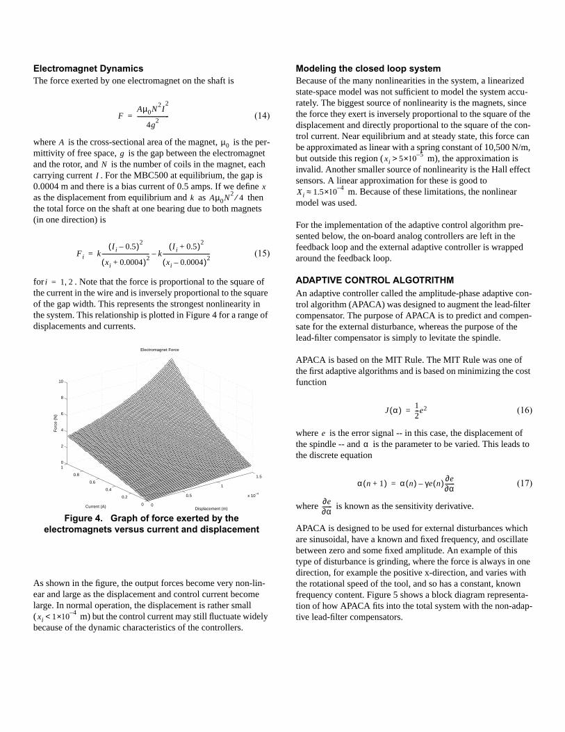
Electromagnet DynamicsThe force exerted by one electromagnet on the shaft is
(14)
where is the cross-sectional area of the magnet, is the per-mittivity of free space, is the gap between the electromagnetand the rotor, and is the number of coils in the magnet, eachcarrying current . For the MBC500 at equilibrium, the gap is0.0004 m and there is a bias current of 0.5 amps. If we defineas the displacement from equilibrium and as thenthe total force on the shaft at one bearing due to both magnets(in one direction) is
(15)
for . Note that the force is proportional to the square ofthe current in the wire and is inversely proportional to the squareof the gap width. This represents the strongest nonlinearity inthe system. This relationship is plotted in Figure 4 for a range ofdisplacements and currents.
Figure 4. Graph of force exerted by theelectromagnets versus current and displacement
As shown in the figure, the output forces become very non-lin-ear and large as the displacement and control current becomelarge. In normal operation, the displacement is rather small( m) but the control current may still fluctuate widelybecause of the dynamic characteristics of the controllers.
FAµ0N
2I
2
4g2
-----------------------=
A µ0g
NI
xk Aµ0N
24⁄
Fi kIi 0.5–( )2
xi 0.0004+( )2---------------------------------- k
Ii 0.5+( )2
xi 0.0004–( )2----------------------------------–=
i 1 2,=
0
0.5
1
1.5
x 10−4
0
0.2
0.4
0.6
0.8
10
2
4
6
8
10
Displacement (m)
Electromagnet Force
Current (A)
For
ce (
N)
xi 14–×10<
Modeling the closed loop systemBecause of the many nonlinearities in the system, a linearizedstate-space model was not sufficient to model the system accu-rately. The biggest source of nonlinearity is the magnets, sincethe force they exert is inversely proportional to the square of thedisplacement and directly proportional to the square of the con-trol current. Near equilibrium and at steady state, this force canbe approximated as linear with a spring constant of 10,500 N/m,but outside this region ( m), the approximation isinvalid. Another smaller source of nonlinearity is the Hall effectsensors. A linear approximation for these is good to
m. Because of these limitations, the nonlinearmodel was used.
For the implementation of the adaptive control algorithm pre-sented below, the on-board analog controllers are left in thefeedback loop and the external adaptive controller is wrappedaround the feedback loop.
ADAPTIVE CONTROL ALGOTRITHMAn adaptive controller called the amplitude-phase adaptive con-trol algorithm (APACA) was designed to augment the lead-filtercompensator. The purpose of APACA is to predict and compen-sate for the external disturbance, whereas the purpose of thelead-filter compensator is simply to levitate the spindle.
APACA is based on the MIT Rule. The MIT Rule was one ofthe first adaptive algorithms and is based on minimizing the costfunction
(16)
where is the error signal -- in this case, the displacement ofthe spindle -- and is the parameter to be varied. This leads tothe discrete equation
(17)
where is known as the sensitivity derivative.
APACA is designed to be used for external disturbances whichare sinusoidal, have a known and fixed frequency, and oscillatebetween zero and some fixed amplitude. An example of thistype of disturbance is grinding, where the force is always in onedirection, for example the positive x-direction, and varies withthe rotational speed of the tool, and so has a constant, knownfrequency content. Figure 5 shows a block diagram representa-tion of how APACA fits into the total system with the non-adap-tive lead-filter compensators.
xi 55–×10>
Xi 1.54–×10≈
J α( ) 12---e2=
eα
α n 1+( ) α n( ) γe n( ) ∂e∂α-------–=
∂e∂α-------
Figure 5. Block diagram including adaptive controller
APACA calculates successive estimates of the amplitude andphase of a complimentary input sine wave that will combinewith the disturbance to create zero net motion. The signal fromthe adaptive controller must go through the amplifier and mag-net dynamics before driving the spindle motion through thebearing magnets. Therefore even if the exact disturbance timehistory is known, it cannot simply be inverted and used directlyto cancel itself out. Also, in grinding applications, the amplitudeof the disturbance may not be known, but the frequency mostlikely will be. If the frequency is not known, it can be deter-mined by using an FFT (fast Fourier transform) algorithm onthe output signal to determine the dominant frequencies, andthen those frequencies can be used in APACA.
Two parameters are varied in determining the output ofAPACA; the amplitude of the wave and the phase shift fromthe disturbance wave (actually computed as a time delaywhere ). The output then looks like
(18)
where is the frequency of the disturbance and is assumed tobe known.
The two variable parameters are calculated according to a modi-fied MIT Rule. The sensitivity derivative is replaced by the timederivative of the error signal in the time delay equation and by aconstant in the amplitude equation (which is absorbed by theconstant ). The error signal in the time delay equation isreplaced by the disturbance signal. These modifications lead tothe recursive equations which form the basis of APACA,
(19)
(20)
SpindleDynamics
MagnetDynamics
Hall-effectSensors
Lead-FilterCompensators
CurrentAmplifiers Force
Displacement of spindle
Input
External Force
VoltageOutputVoltage
AdaptiveControllers
+
+
+-
AT
φ ωT=
yA A ωt ωT+( )sin 1+( )=
ω
γA
A n 1+( ) A n( ) γAe n( )+=
T n 1+( ) T n( ) γTde n( )
dt--------------d n( )+=
SIMULATION AND HARWAREThese equations were implemented in Simulink using theparameters shown in Table 3.
These parameters were found through testing the controller insimulation and on the experimental setup and trying to find abalance between short convergence time and stability. Like theMIT Rule, a poor selection for and (a value that is toolarge) may result in system instability. However, values that aretoo small will result in long convergence times and a system thatwon’t be able to adapt to changing disturbances.
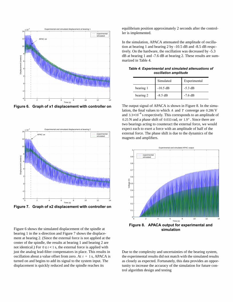
RESULTSThe system was tested in simulation with a disturbance input of0.5 N and frequency of 100 Hz. On the hardware, this corre-sponded to an input current of 2.3 amps. The results are shownin the following figures. In order to increase the stability of thesystem, APACA is not implemented in the simulation until afterthe transient rigid body motion has been damped out by the on-board analog controllers. The time at which APACA is turnedon is marked on the plots. The maximum range of the spindlemotion is m, but normal operating range is
m, so the displacement of the spindle shown inFigure 6 and Figure 7 is near the limit of the normal operatingrange. There was a small amount of noise injected into the cur-rent amplifier signal in the simulation in order to determine itseffects on the adaptation algorithm. The power of this noise wasdetermined from steady-state experimental data.
Table 3: Simulation parameters
parameter value
sample time ms
γA 15–×10
γT 19–×10
0.1
γA γT
405–×10±
155–×10±
Figure 6. Graph of x1 displacement with controller on
Figure 7. Graph of x2 displacement with controller on
Figure 6 shows the simulated displacement of the spindle atbearing 1 in the x-direction and Figure 7 shows the displace-ment at bearing 2. (Since the external force is not applied at thecenter of the spindle, the results at bearing 1 and bearing 2 arenot identical.) For s, the external force is applied withjust the analog lead-filter compensators in place. This results inoscillation about a value offset from zero. At s, APACA isturned on and begins to add its signal to the system input. Thedisplacement is quickly reduced and the spindle reaches its
0 2 4 6 8 10 12 14−4
−2
0
2
4
6
8
10
12
14x 10
−5 Experimental and simulated displacement at bearing 1
Time (s)
Dis
plac
emen
t (m
eter
s)
experimentalsimulated
APAC on
0 2 4 6 8 10 12 14−4
−2
0
2
4
6
8
10
12
14x 10
−5 Experimental and simulated displacement at bearing 2
Time (s)
Dis
plac
emen
t (m
eter
s)
experimentalsimulated
APAC on
0 t 1<≤
t 1=
equilibrium position approximately 2 seconds after the control-ler is implemented.
In the simulation, APACA attenuated the amplitude of oscilla-tion at bearing 1 and bearing 2 by -10.5 dB and -8.5 dB respc-tively. On the hardware, the oscillation was decreased by -5.3dB at bearing 1 and -7.6 dB at bearing 2. These results are sum-marized in Table 4.
The output signal of APACA is shown in Figure 8. In the simu-lation, the final values to which and converge are Vand s respectively. This corresponds to an amplitude of
N and a phase shift of rad, or . Since there aretwo bearings acting to counteract the external force, we wouldexpect each to exert a force with an amplitude of half of theexternal force. The phase shift is due to the dynamics of themagnets and amplifiers.
Figure 8. APACA output for experimental andsimulation
Due to the complexity and uncertainties of the bearing system,the experimental results did not match with the simulated resultsas closely as expected. Fortunately, this data provides an oppor-tunity to increase the accuracy of the simulation for future con-trol algorithm design and testing
Table 4: Experimental and simulated attenuations ofoscillation amplitude
Simulated Experimental
bearing 1 -10.5 dB -5.3 dB
bearing 2 -8.5 dB -7.6 dB
A T 0.2863.3
4–×10
0.25 0.033 1.9°
0 2 4 6 8 10 12 140
0.1
0.2
0.3
0.4
0.5
0.6
0.7
0.8
0.9
1Experimental and simulated APAC output
Time (s)
Vol
tage
(V
)
experimentalsimulated
CONCLUSION AND FUTURE WORKThe two parameter adaptive control algorithm presented hereyielded considerable reduction in steady-state displacement inboth simulation and experiment for an externally applied sinu-soidal load. Future enhancements to the current design willinclude four parameters to adjust in the output; the amplitude ofthe sine wave, the frequency of the sine wave, the phase shift,and the offset from zero. These enhancements will allow thealgorithm to handle a constant disturbance, a sine wave oscillat-ing about zero, or a sine wave of unknown or slowly varyingfrequency.
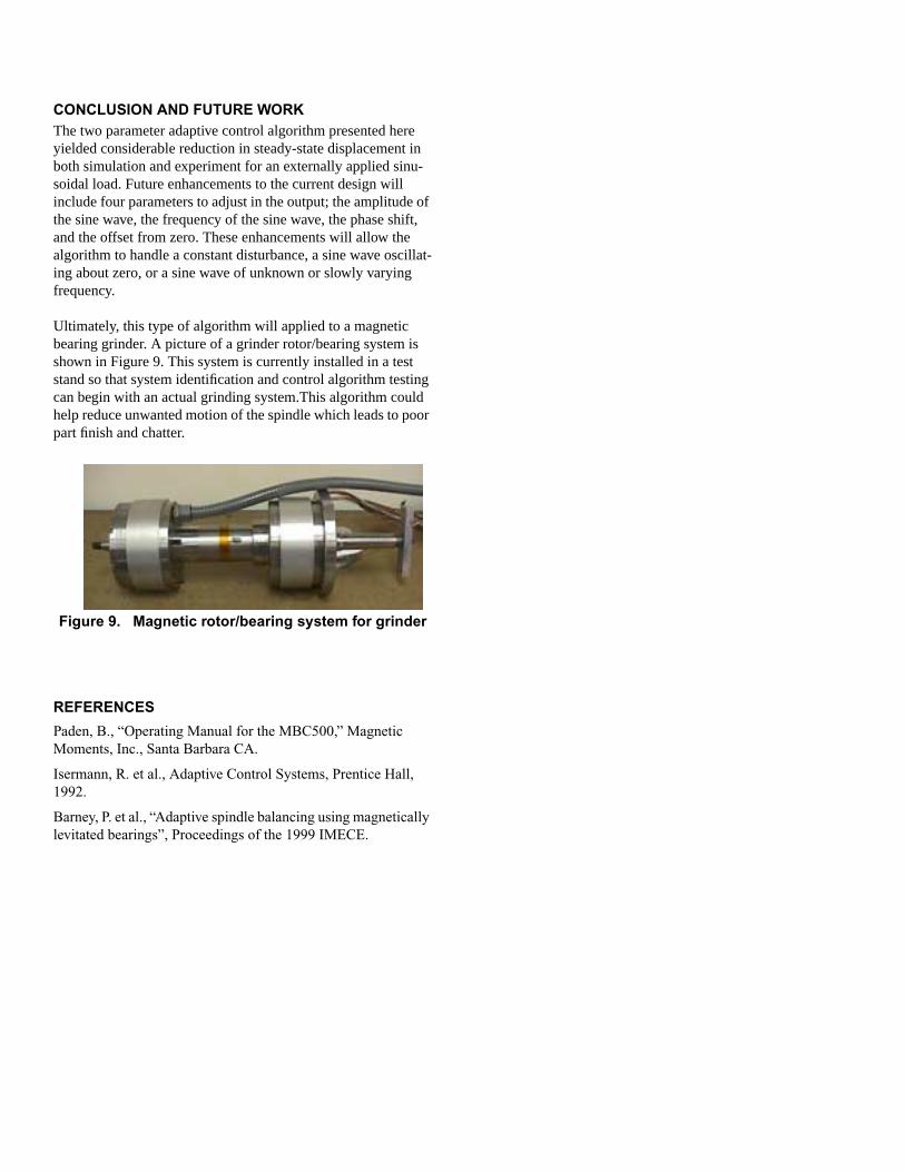
Ultimately, this type of algorithm will applied to a magneticbearing grinder. A picture of a grinder rotor/bearing system isshown in Figure 9. This system is currently installed in a teststand so that system identification and control algorithm testingcan begin with an actual grinding system.This algorithm couldhelp reduce unwanted motion of the spindle which leads to poorpart finish and chatter.
Figure 9. Magnetic rotor/bearing system for grinder
REFERENCES
Paden, B., “Operating Manual for the MBC500,” Magnetic
Moments, Inc., Santa Barbara CA.
Isermann, R. et al., Adaptive Control Systems, Prentice Hall,
1992.
Barney, P. et al., “Adaptive spindle balancing using magnetically
levitated bearings”, Proceedings of the 1999 IMECE.
Distribution
MS 0557 Thomas J. Baca (09125)MS 0501 Patrick S. Barney (02338)
(5 copies)MS 0841 Tomas C. Bickel (09100)MS 0509 Michael W. Callahan (02300)MS 0960 Norman E. Demeza (14100)MS 9405 Michal T. Dyer (08700)MS 0555 Mark S. Garrett (09122)MS 9042 James L. Handrock (08727)MS 0501 Ming K. Lau(2338)MS 9042 James P. Lauffer (08727)
(5 copies)MS 0847 David M. Martinez (09124)MS0847 Rodney A. May (09126)MS0188 Charles E. Meyers (01030)MS 0847 Harold S. Morgan (09123)MS 0958 Alan R. Parker (14184)MS 0847 James M. Redmond (09124)
(5 copies)MS 0958 William N. Sullivan (14184)
(5 copies)MS 0899 Tech Library (09616)
(2 copies)MS 0612 Review and Approval Desk (9612)
for DOE/OSTI(1 copies)
MS 9018 Central Technical Files (8945-1)
Prof. Brad PadenMagnetic Moments, Inc5735 Hollister Avenue, Suite BGoleta, CA 93117Santa Barbara, CA
Prof. Gordon ParkerMichigan Technical University1400 Townsend Dr.Houghton, MI 49931(5 copies)