Active Structural Control- Intelligent Control -

Hyun Myung, Ph.D.Dept. of Civil & Env. EnggKAIST Robotics Programhmyung@kaist.ac.kr http://web.kaist.ac.kr/~ceerobot

Asia-Pacific Student Summer School 2008

Active Control

• Passive Control

▫ Inexpensive

▫ No external energy

▫ Inherently stable

▫ It works even during a major earthquake

• Active Control

▫ Can deal with dynamic structural variations, disturbances

▫ External power is used to effect the control action

▫ Vulnerable to power failure (possible during strong earthquake)

▫ Can destabilize if the implementation errors are serious enough

2

Types of Active Control

• Adaptive Control

• Stochastic Control

▫ (Extended) Kalman Filter

▫ Particle Filter

• Intelligent Control

▫ Neural Networks

▫ Fuzzy Logic

▫ Neuro-Fuzzy

▫ Genetic Algorithms

• Sliding Mode Control

• Optimal Control

• Robust Control

3

Adaptive Control

• Modify control law used by a controller

▫ the parameters of the system being controlled are slowly time-varying or uncertain

4

Indirect Adaptive Control Direct Adaptive Control

Model Reference Adaptive Control

5

Model Reference Adaptive Control

Indirect MRAC Direct MRAC

Stochastic Control: Kalman Filter

• Given the linear dynamical system:

)(),( matrices covariance

(known) with noiseGaussian whitemean,-zero are )(),(

(known) matrices system ddimensioneely appropriat are )(),(),(

measured) (known,tor output vec ldimensiona- theis )(

(known)or input vect ldimensiona- theis )(

(unknown) vector state ldimensiona- theis )(

kRkQ

kwkv

kHkGkF

pky

mku

nkx

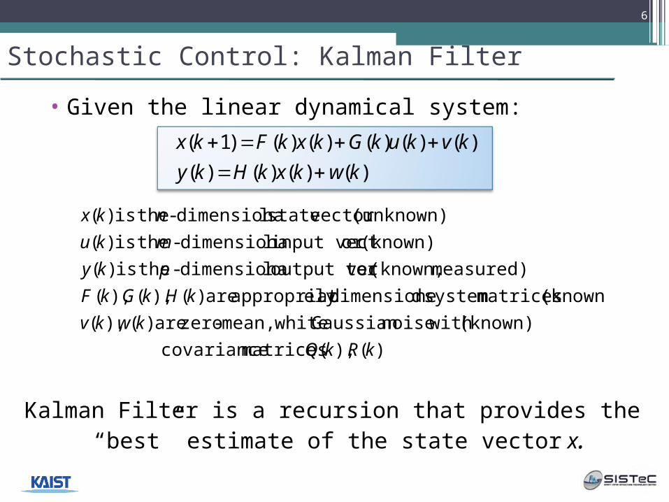
Kalman Filter is a recursion that provides the “best” estimate of the state vector x.

)()()()(

)()()()()()1(

kwkxkHky

kvkukGkxkFkx

6

How does it work?

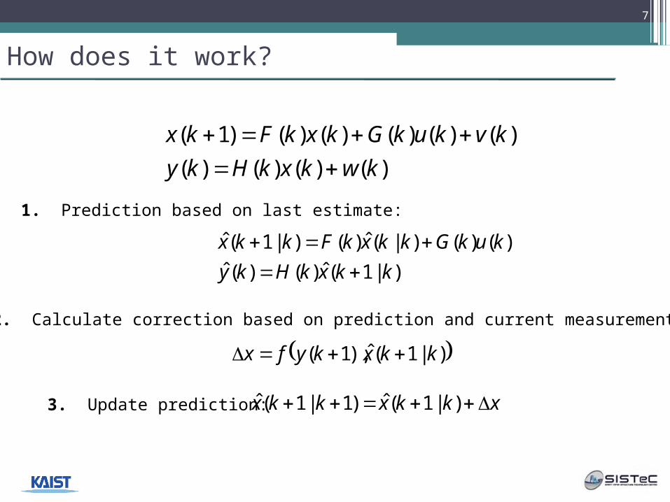
x k F k x k G k u k v k

y k H k x k w k

( ) ( ) ( ) ( ) ( ) ( )

( ) ( ) ( ) ( )

1

)|1(ˆ)()(ˆ

)()()|(ˆ)()|1(ˆ

kkxkHky

kukGkkxkFkkx

1. Prediction based on last estimate:

2. Calculate correction based on prediction and current measurement:

)|1(ˆ),1( kkxkyfx

3. Update prediction: xkkxkkx )|1(ˆ)1|1(ˆ

7

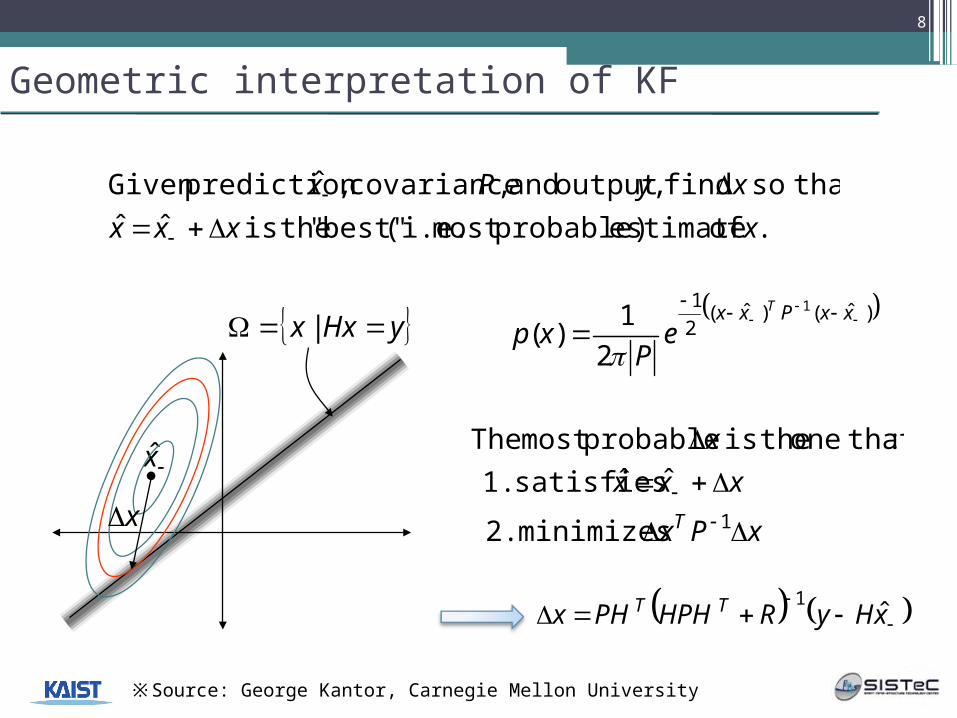
Geometric interpretation of KF

)ˆ()ˆ(2

1 1

2

1)(

xxPxx T

eP

xp

. of estimate probable)most (i.e. best"" theis ˆˆ

that so find ,output and , covariance ,ˆ predictionGiven

xxxx

xyPx

yHxx |

x̂

x xPx

xxx

x

T

1 minimizes 2.

ˆˆ satisfies 1.

: thatone theis probablemost The

8

※Source: George Kantor, Carnegie Mellon University

xHyRHPHPHx TT ˆ1

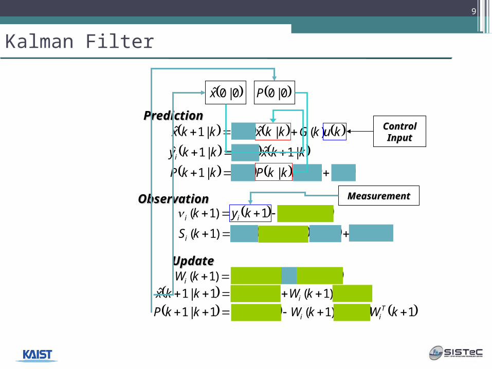
Kalman Filter

kukGkkxkFkkx )(|ˆ|1ˆ

kkxkHkky ii |1ˆ|1ˆ

kQkFkkPkFkkP T ||1

kkykyk iii |1ˆ1)1(

1|1)1( kRkHkkPkHkS iTiii

1)1(|1ˆ1|1ˆ kkWkkxkkx ii 11)1(|11|1 kWkSkWkkPkkP T

ii

1|1)1( 1 kSHkkPkW iTii

0|0x̂ 0|0P

Control Control InputInput

MeasuremenMeasurementt

PredictionPrediction

ObservationObservation

UpdateUpdate

9

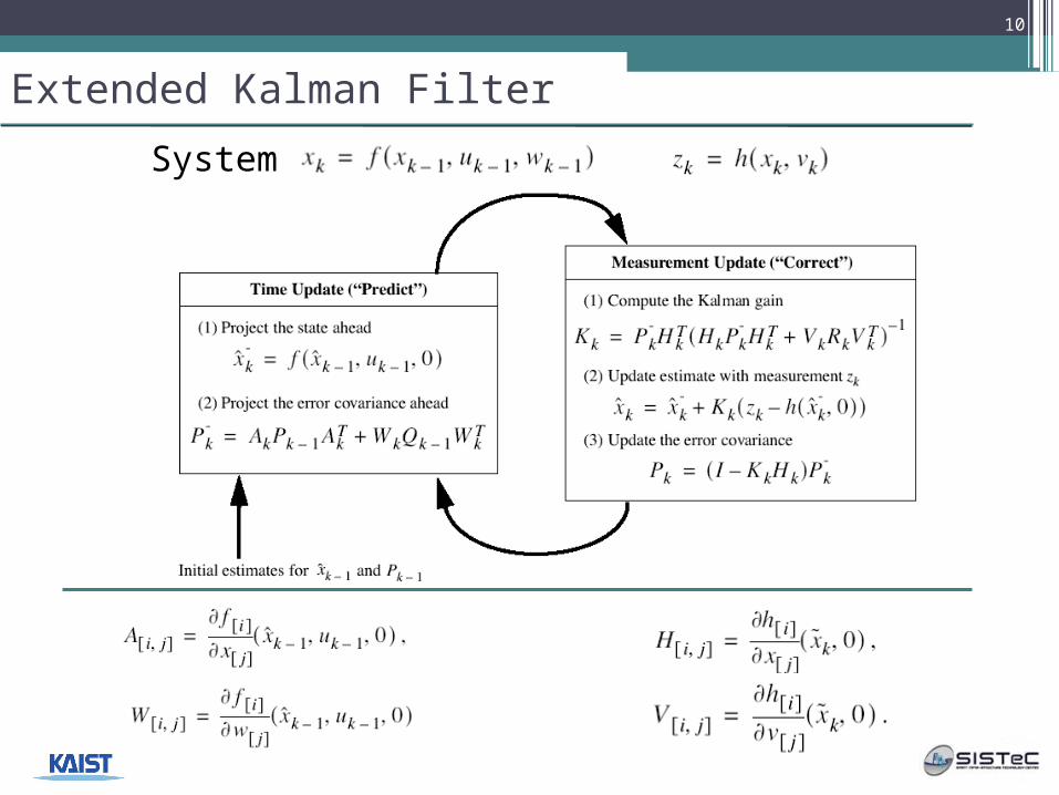
Extended Kalman Filter

System:

10

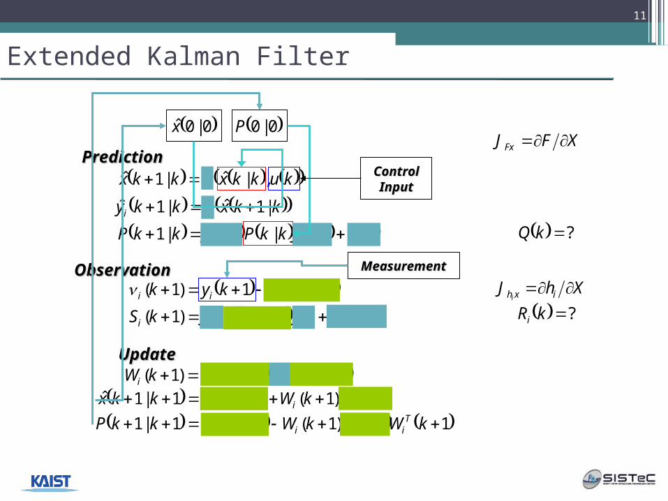
Extended Kalman Filter

kukkxFkkx ,|ˆ|1ˆ

kkxhkky ii |1ˆ|1ˆ

kQkJkkPkJkkP TFxFx ||1

kkykyk iii |1ˆ1)1( 1|1)1( kRJkkPJkS i

Txhxhi ii

1)1(|1ˆ1|1ˆ kkWkkxkkx ii 11)1(|11|1 kWkSkWkkPkkP T

ii

1|1)1( 1 kSHkkPkW iTii

0|0x̂ 0|0P

Control Control InputInput

MeasuremenMeasurementt

PredictionPrediction

ObservationObservation

UpdateUpdate

XFJ Fx

XhJ ixhi

?kQ

?kRi

11

Stochastic Control: Particle Filter - Motivation

• The trend of addressing complex problems continues

• Large number of applications require evaluation of integrals

• Non-linear models

• Non-Gaussian noise

12

※Reference: M. S. Arulampalam, S. Maskell, N. Gordon, and T. Clapp, “A tutorial on particle filters for online nonlinear/non-gaussian Bayesian tracking,” IEEE Transactions on Signal Processing, vol. 50, no. 2, pp. 174–188, 2002.

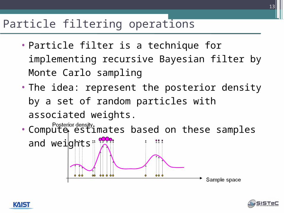
Particle filtering operations

• Particle filter is a technique for implementing recursive Bayesian filter by Monte Carlo sampling

• The idea: represent the posterior density by a set of random particles with associated weights.

• Compute estimates based on these samples and weights

13

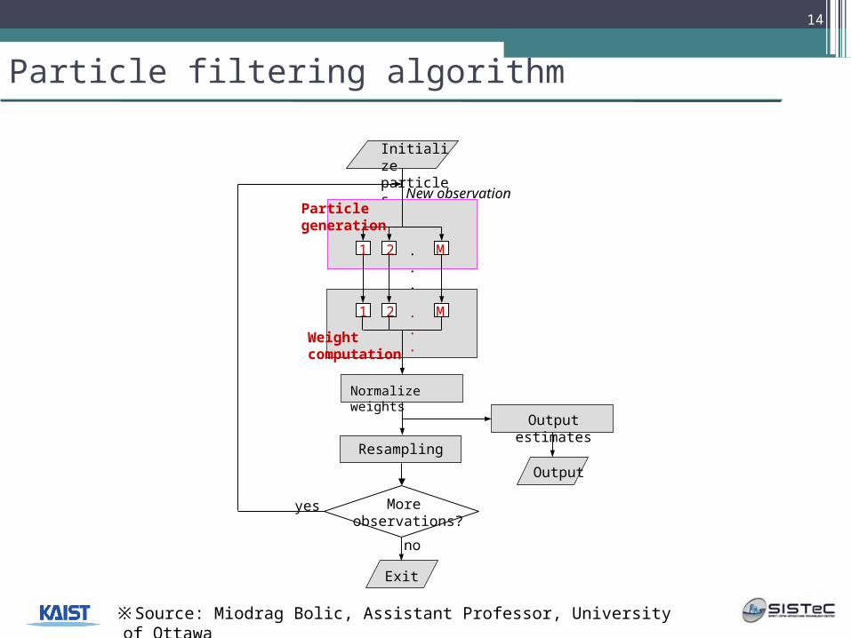
Particle filtering algorithm

14

Initialize particles

Output

Output estimates

1 2 M. . .

Particlegeneration

New observation

Exit

Normalize weights

1 2 M. . .Weight

computation

Resampling

More observations?

yes

no

※Source: Miodrag Bolic, Assistant Professor, University of Ottawa

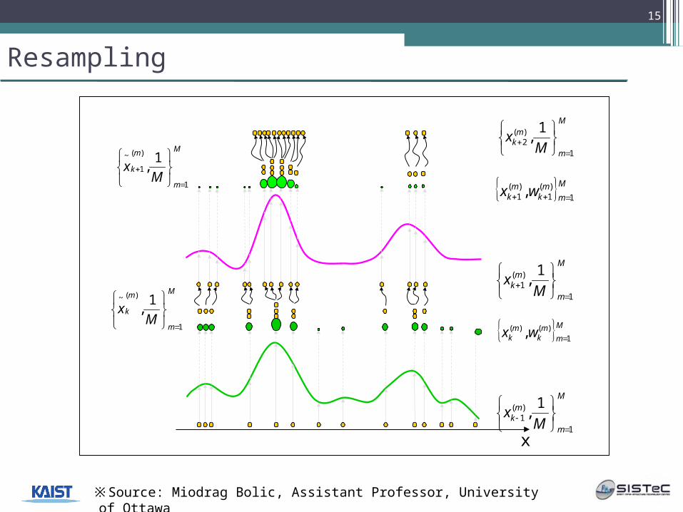
Resampling

M

m

mk M

x1

)(1

1,

x

M

mm

km

k wx 1)()( ,

M

m

m

kM

x1

)(~ 1,

M

m

mk M

x1

)(1

1,

M

mm

km

k wx 1)(1

)(1 ,

M

m

m

kM

x1

)(

1

~ 1,

M

m

mk M

x1

)(2

1,

15

※Source: Miodrag Bolic, Assistant Professor, University of Ottawa

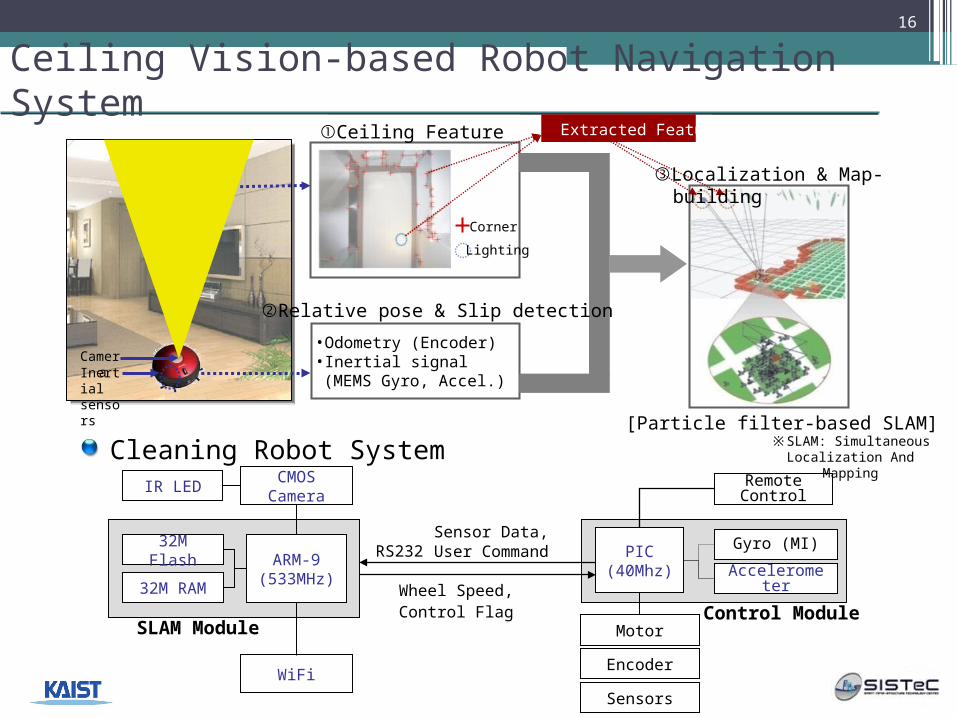
Ceiling Vision-based Robot Navigation System

[Particle filter-based SLAM]

•Odometry (Encoder)•Inertial signal (MEMS Gyro, Accel.)

Extracted Features①Ceiling Feature Extraction

Camera

Cleaning Robot System

ARM-9(533MHz

)

32M Flash

32M RAM

PIC(40Mhz)

Wheel Speed,Control Flag

Sensor Data,User

Command

CMOS Camera

Encoder

Gyro (MI)

Sensors

Accelerometer

Motor

Remote Control

WiFi

RS232

IR LED

SLAM ModuleControl Module

Inertial sensors

Corner

Lighting

③Localization & Map-building

②Relative pose & Slip detection

16

※SLAM: Simultaneous Localization And

Mapping

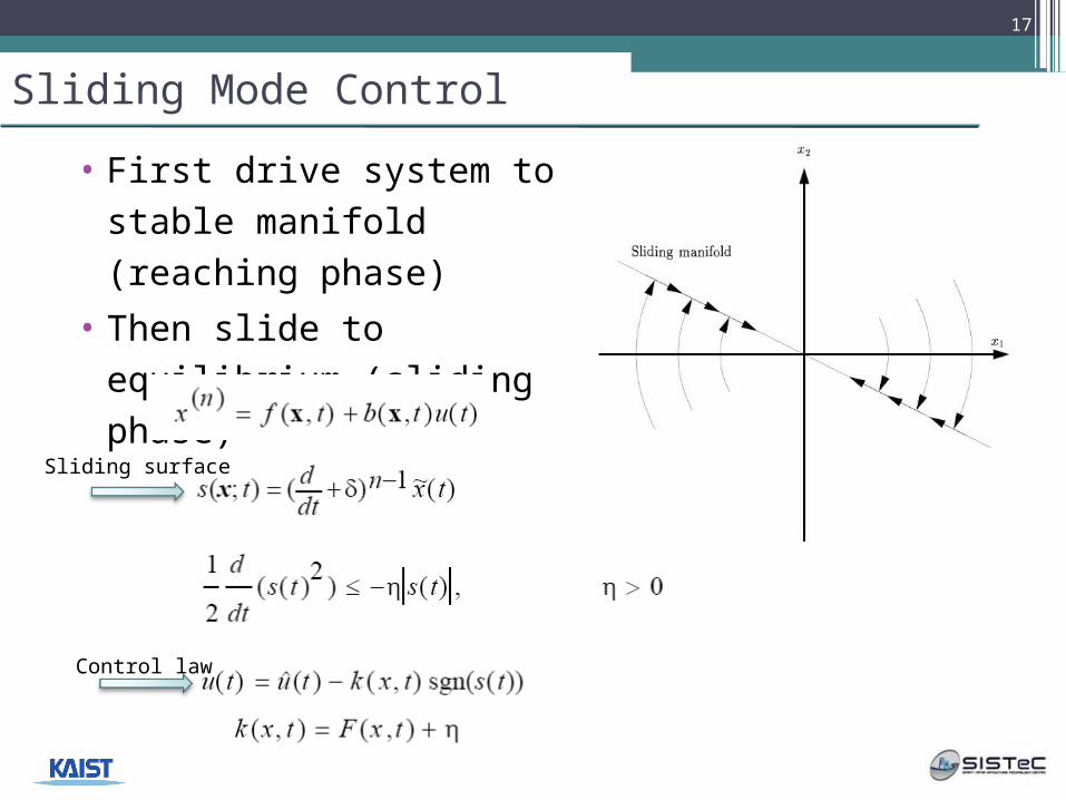
Sliding Mode Control

• First drive system to stable manifold (reaching phase)

• Then slide to equilibrium (sliding phase)

17

Control law

Sliding surface

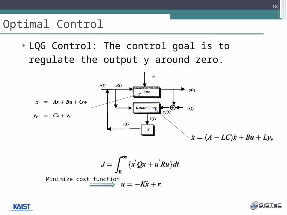
Optimal Control

• LQG Control: The control goal is to regulate the output y around zero.

18

Minimize cost function

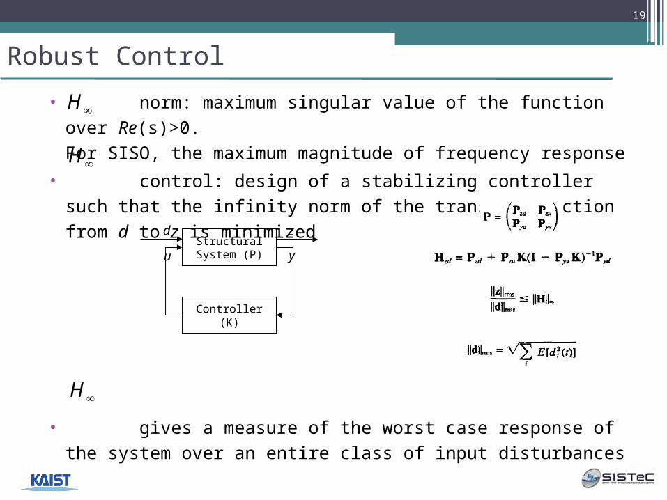
Robust Control

• norm: maximum singular value of the function over Re(s)>0. For SISO, the maximum magnitude of frequency response

• control: design of a stabilizing controller such that the infinity norm of the transfer function from d to z is minimized

• gives a measure of the worst case response of the system over an entire class of input disturbances

19

H

H

Structural System (P)

Controller (K)

d

u y

z

H

Eye Fusion

20

Intelligent Control

• Neural networks-based control

• Fuzzy logic control

• Neuro-fuzzy control

• GA-neuro control

• GA-fuzzy control

21

22

Biological inspirations

• Some numbers…

▫The human brain contains about 10 billion nerve cells (neurons)

▫Each neuron is connected to the others through 10,000 synapses

• Properties of the brain

▫It can learn, reorganize itself from experience

▫It adapts to the environment

▫It is robust and fault tolerant

23

Definition: Artificial Neural Network

• An analysis paradigm very roughly modeled after

the massively parallel structure of the brain.

• Simulates a highly interconnected, parallel computational structure with numerous relatively simple individual processing elements.

• Some differences between biological and artificial neurons (processing elements):

▫ Signs of weights (+ or -)

▫ Signals are AC in neurons, DC in PES

▫ Many types of neurons in a system; usually only a few at most in neural networks

▫ Basic cycle time for PC (~100 ns) faster than brain (10-100ms) {as far as we know!}

24

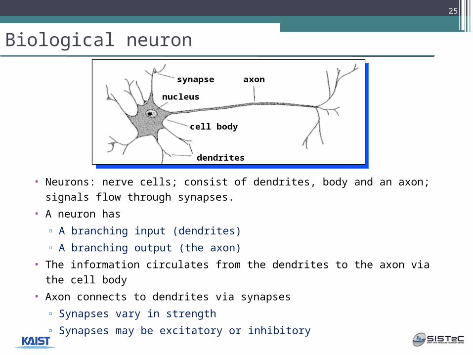
Biological neuron

• Neurons: nerve cells; consist of dendrites, body and an axon; signals flow through synapses.

• A neuron has

▫ A branching input (dendrites)

▫ A branching output (the axon)

• The information circulates from the dendrites to the axon via the cell body

• Axon connects to dendrites via synapses

▫ Synapses vary in strength

▫ Synapses may be excitatory or inhibitory

25

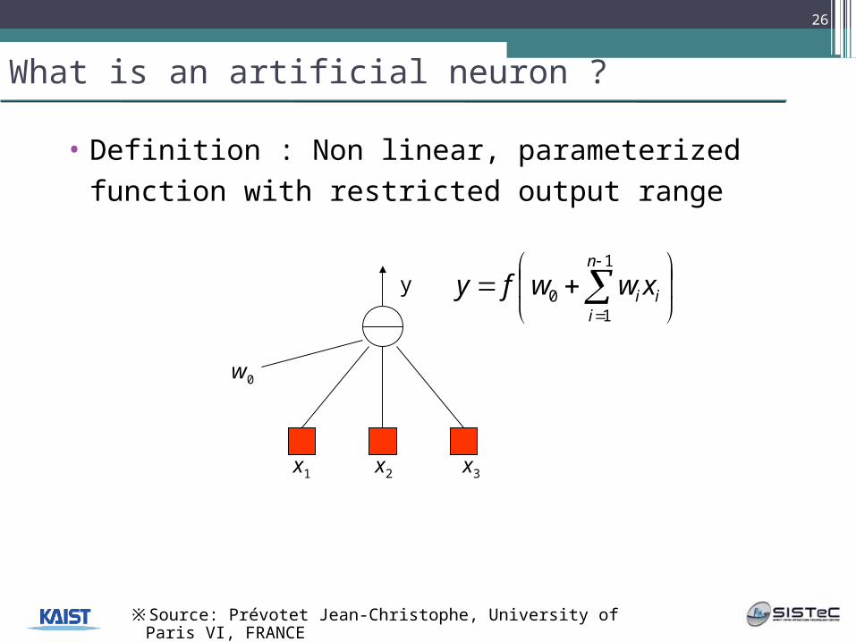
What is an artificial neuron ?

1

10

n

iii xwwfy

• Definition : Non linear, parameterized function with restricted output range

x1 x2 x3

w0

y

26

※Source: Prévotet Jean-Christophe, University of Paris VI, FRANCE

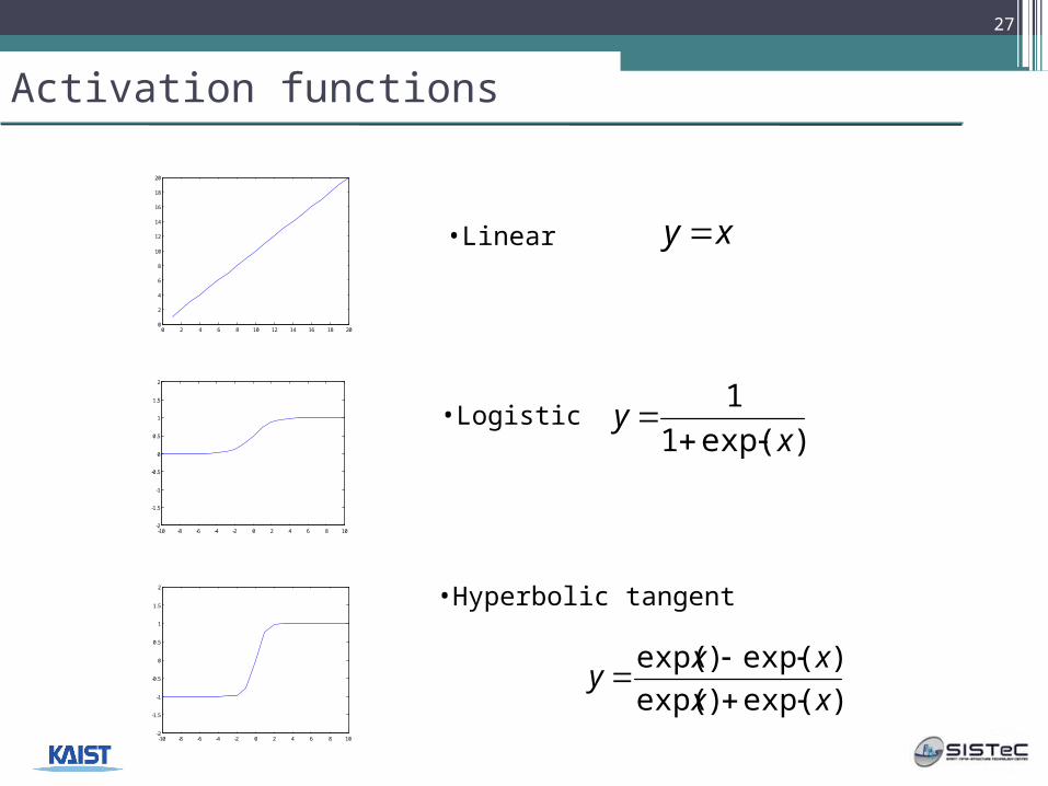
Activation functions

-10 -8 -6 -4 -2 0 2 4 6 8 10-2

-1.5

-1

-0.5

0

0.5

1

1.5

2

-10 -8 -6 -4 -2 0 2 4 6 8 10-2

-1.5

-1

-0.5

0

0.5

1

1.5

2

xy

0 2 4 6 8 10 12 14 16 18 200

2

4

6

8

10

12

14

16

18

20

•Linear

•Logistic

•Hyperbolic tangent

)exp(1

1

xy

)exp()exp(

)exp()exp(

xx

xxy

27

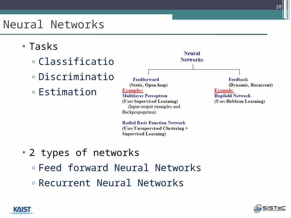
Neural Networks

• Tasks

▫Classification

▫Discrimination

▫Estimation

• 2 types of networks

▫Feed forward Neural Networks

▫Recurrent Neural Networks

28

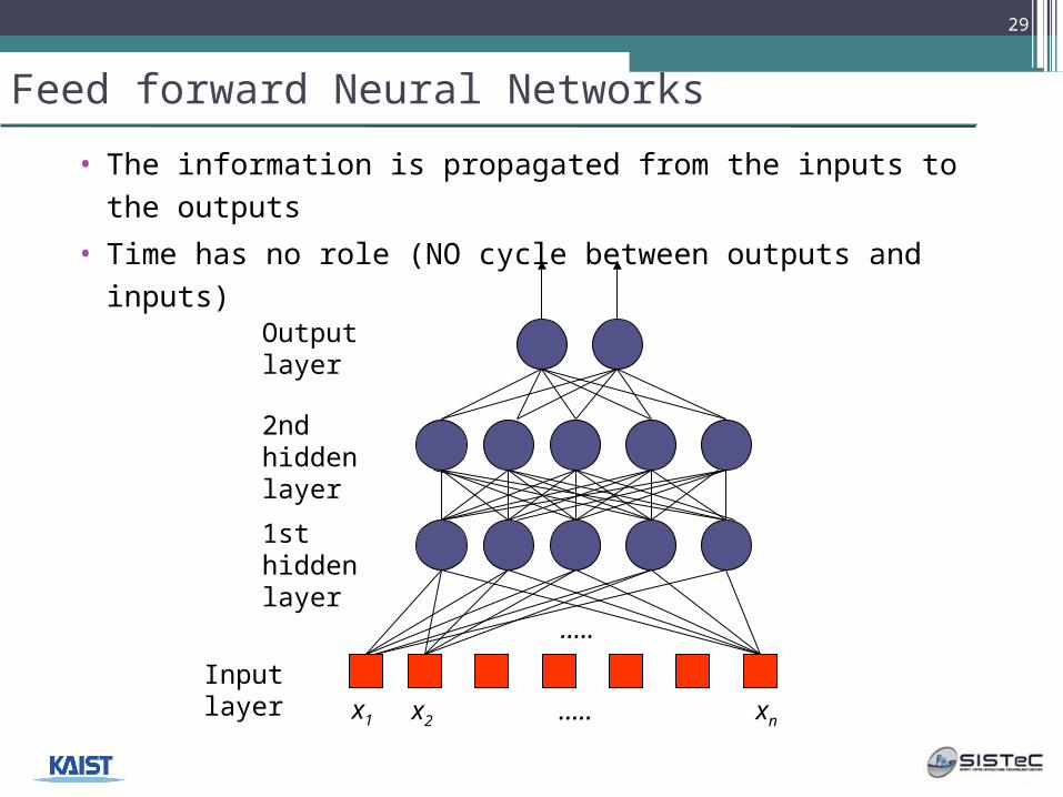
Feed forward Neural Networks

• The information is propagated from the inputs to the outputs

• Time has no role (NO cycle between outputs and inputs)

29

x1 x2 xn…..

1st hidden layer

2nd hiddenlayer

Output layer

Input layer

…..

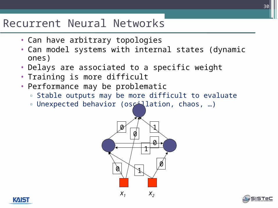
Recurrent Neural Networks• Can have arbitrary topologies• Can model systems with internal states (dynamic ones)• Delays are associated to a specific weight• Training is more difficult• Performance may be problematic

▫ Stable outputs may be more difficult to evaluate▫ Unexpected behavior (oscillation, chaos, …)

x1 x2

1

010

10

00

30

Learning

• The procedure that consists in estimating the parameters of neurons so that the whole network can perform a specific task

• 2 types of learning

▫ The supervised learning

▫ The unsupervised learning

• The Learning process (supervised)

▫ Present the network a number of inputs and their corresponding outputs

▫ See how closely the actual outputs match the desired ones

▫ Modify the parameters to better approximate the desired outputs

31

Supervised learning

• The desired response of the neural network in function of particular inputs is well known.

• A “Teacher” may provide examples and teach the neural network how to fulfill a certain task

32

Unsupervised learning

• Idea : group typical input data in function of resemblance criteria unknown a priori

• Data clustering

• No need of a teacher

▫The network finds itself the correlations between the data

▫Examples of such networks Kohonen feature maps: Competitive learning

33

Classical neural architectures

• Perceptron

• Multi-layer Perceptron

• Radial Basis Function (RBF)

• Kohonen features maps

• Other architectures

▫Shared weights neural networks

▫ART: Adaptive Resonance Theory

▫Cascading neural networks

34

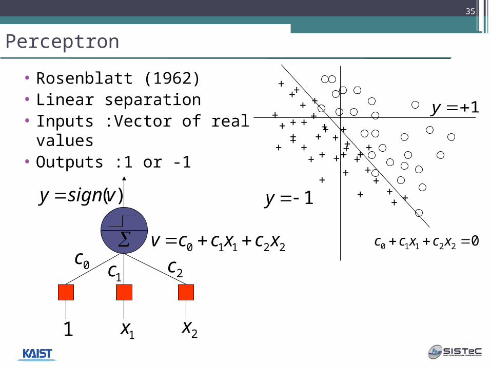
Perceptron

• Rosenblatt (1962)• Linear separation• Inputs :Vector of real

values• Outputs :1 or -1

022110 xcxcc

1y

+ +++

++

++

++ + +

++ +

+

+++

++

+

++

++

+++

++

+

+

+

+

+

1y

0c1c 2c

1x 2x1

22110 xcxccv

)(vsigny

35

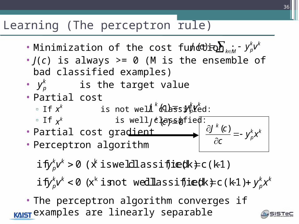
Learning (The perceptron rule)

Mk

kkpvycJ )(• Minimization of the cost function :

• J(c) is always >= 0 (M is the ensemble of bad classified examples)

• is the target value • Partial cost

▫ If is not well classified:▫ If is well classified:

• Partial cost gradient• Perceptron algorithm

• The perceptron algorithm converges if examples are linearly separable

kx

kpy

kkp

kkp

kkp

xyvy

vy

1)-c(kc(k) :)classified not well is x( 0 if

1)-c(kc(k) :)classified wellis (x 0 ifk

k

kx

kkp

k vycJ )(

0)( cJ k

kkp

k

xyc

cJ

)(

36

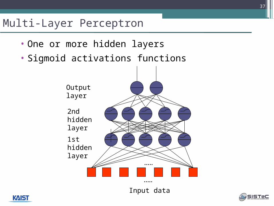
Multi-Layer Perceptron

• One or more hidden layers

• Sigmoid activations functions

1st hidden layer

2nd hiddenlayer

Output layer

Input data

37

…..

…..

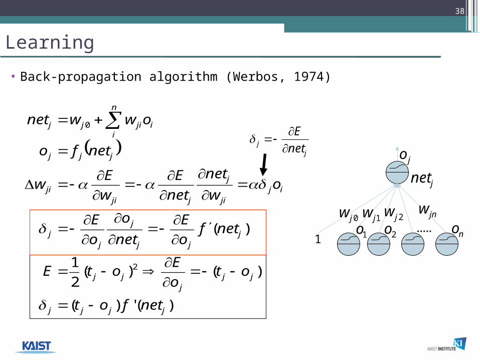
Learning

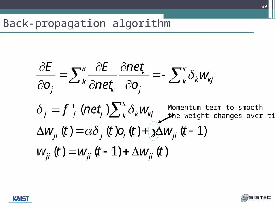
• Back-propagation algorithm (Werbos, 1974)

jj net

E

)(')(

)()(2

1

)(

2

0

jjjj

jjj

jj

jjj

j

jj

ijji

j

jjiji

jjj

n

iijijj

netfot

oto

EotE

netfo

E

net

o

o

E

ow

net

net

E

w

Ew

netfo

owwnet

38

jo

jnet

0jw2o no….

.

1jw 2jw jnw

1o1

)()1()(

)1()()()(

)('

twtwtw

twtottw

wnetf

wo

net

net

E

o

E

jijiji

jiijji

k kjkjjj

k k kjkjj

Momentum term to smooththe weight changes over time

Back-propagation algorithm

39

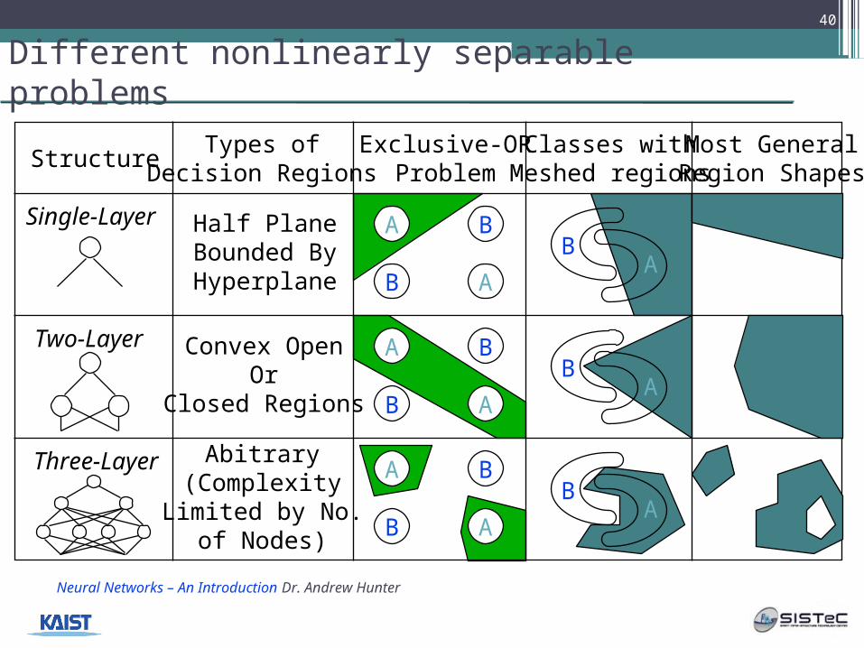
StructureTypes of

Decision RegionsExclusive-OR

ProblemClasses with

Meshed regionsMost General

Region Shapes

Single-Layer

Two-Layer

Three-Layer

Half PlaneBounded ByHyperplane

Convex OpenOr

Closed Regions

Abitrary(Complexity

Limited by No.of Nodes)

A

AB

B

A

AB

B

A

AB

B

BA

BA

BA

Different nonlinearly separable problems

Neural Networks – An Introduction Dr. Andrew Hunter

40

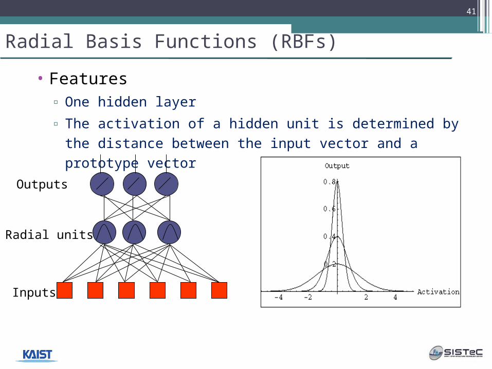
Radial Basis Functions (RBFs)

• Features▫ One hidden layer

▫ The activation of a hidden unit is determined by the distance between the input vector and a prototype vector

Radial units

Outputs

Inputs

41

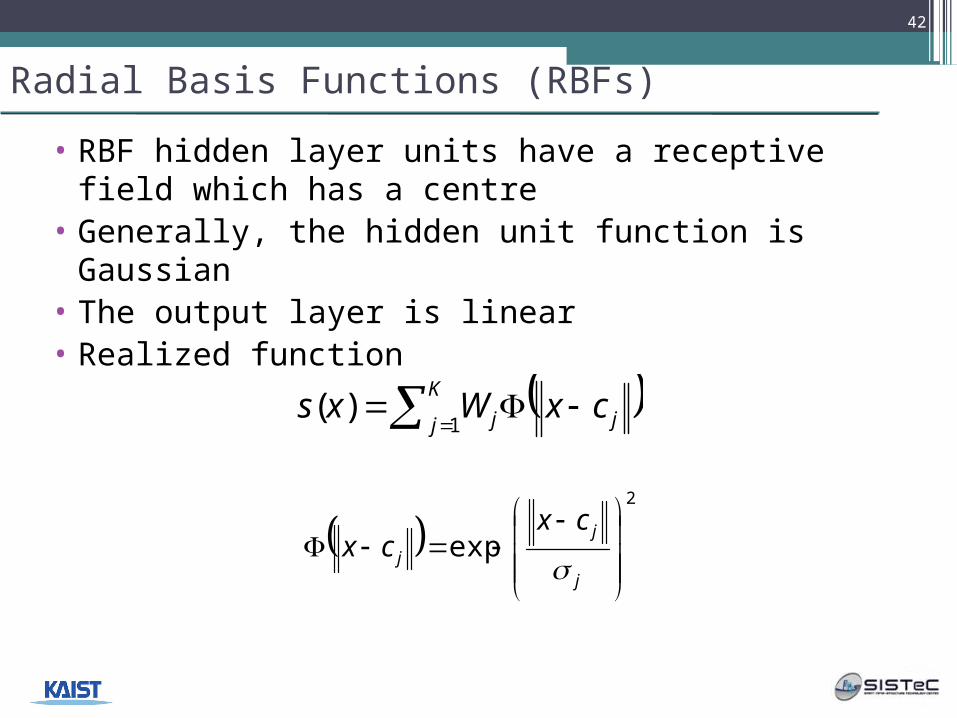
• RBF hidden layer units have a receptive field which has a centre

• Generally, the hidden unit function is Gaussian• The output layer is linear• Realized function

Radial Basis Functions (RBFs)

K

j jj cxWxs1

)(

2

exp

j

j

j

cxcx

42

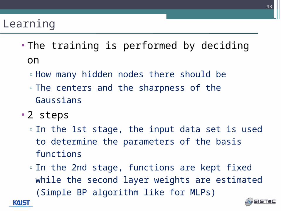
Learning

•The training is performed by deciding on▫How many hidden nodes there should be

▫The centers and the sharpness of the Gaussians

•2 steps▫In the 1st stage, the input data set is used to

determine the parameters of the basis functions

▫In the 2nd stage, functions are kept fixed while the second layer weights are estimated (Simple BP algorithm like for MLPs)

43

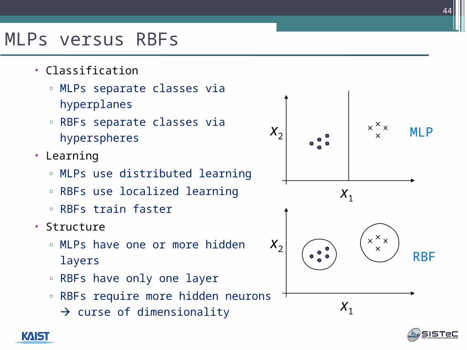
MLPs versus RBFs

• Classification

▫ MLPs separate classes via hyperplanes

▫ RBFs separate classes via hyperspheres

• Learning

▫ MLPs use distributed learning

▫ RBFs use localized learning

▫ RBFs train faster

• Structure

▫ MLPs have one or more hidden layers

▫ RBFs have only one layer

▫ RBFs require more hidden neurons curse of dimensionality

x2

x1

MLP

x2

x1

RBF

44

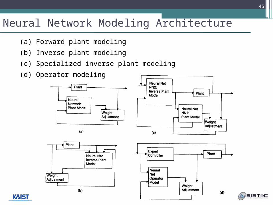
Neural Network Modeling Architecture

(a) Forward plant modeling

(b) Inverse plant modeling

(c) Specialized inverse plant modeling

(d) Operator modeling

45

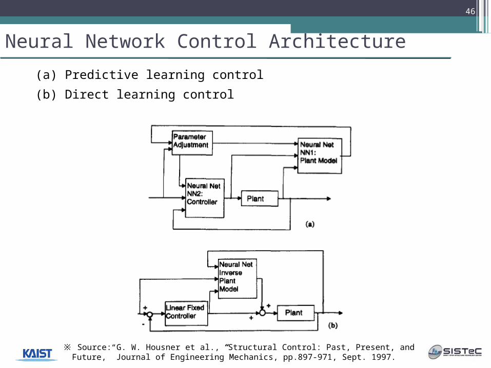
Neural Network Control Architecture

(a) Predictive learning control

(b) Direct learning control

46

※ Source: G. W. Housner et al., “Structural Control: Past, Present, and Future,” Journal of Engineering Mechanics, pp.897-971, Sept. 1997.

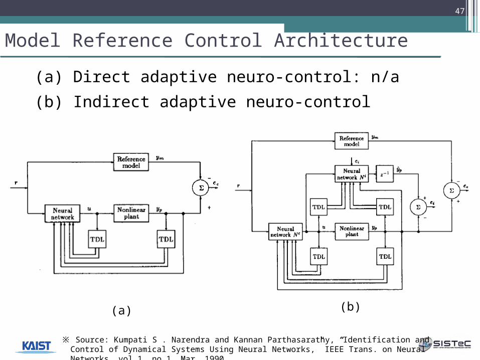
Model Reference Control Architecture

(a) Direct adaptive neuro-control: n/a

(b) Indirect adaptive neuro-control

47

(a) (b)

※ Source: Kumpati S . Narendra and Kannan Parthasarathy, “Identification and Control of Dynamical Systems Using Neural Networks,” IEEE Trans. on Neural Networks, vol.1, no.1, Mar. 1990.

48

Definition: Fuzziness

• Fuzziness: Non-statistical imprecision and vagueness in information and data.

• Fuzzy Sets model the properties of imprecision, approximation or vagueness.

• Fuzzy Membership Values reflect the membership grades in a set.

• Fuzzy Logic is the logic of approximate reasoning. It is a generalization of conventional logic.

49

Fuzzy Logic Behavioral Motivations

• FL analogous to uncertainty in human experiences (“Stop the car pretty soon.”)

• Fuzziness is associated with non-statistical uncertainty

• FL thus is reflected at the behavioral level of the organism

• Fuzziness is not resolved by observation or measurement

50

Application Areas: Fuzzy Logic

• Control systems

▫Vehicles

▫Home appliances

▫Structure

• Expert systems

▫Industrial processes

▫Diagnostics

▫Finance

▫Robotics and manufacturing

51

Fuzzy Sets

• Proposed by Ladeh Zadeh in 1965

▫"Fuzzy sets," Information and Control, vol. 8, pp. 338--353, 1965.

• A generalization of set theory that allows partial membership in a set.

▫Membership is a real number with a range [0, 1]

▫Membership functions are commonly triangular or Gaussian because ease of computation.

▫Utility comes from overlapping membership functions – a value can belong to more than one set

52

52

※Source: Dr. Stephen Paul Linder

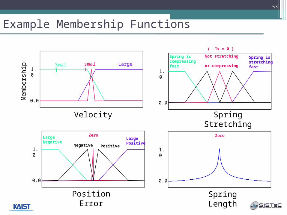
Example Membership Functions

53

1.0

0.0

Spring Stretching

small

LargeSmall

Mem

bers

hi

p

1.0

0.0

Not stretching or compressing

Spring is stretching fast

Spring is compressing fast

Position Error

1.0

ZeroLarge Negative

Velocity

Large Positive Negative Positive

0.0

( x = 0 )

Spring Length

1.0

Zero

0.0

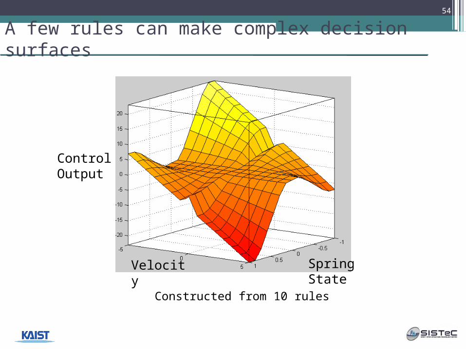
A few rules can make complex decision surfaces

54

Velocity Spring State

Control Output

Constructed from 10 rules

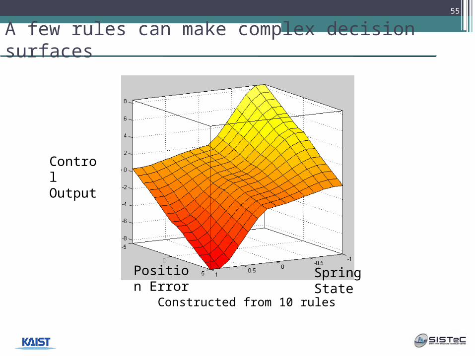
A few rules can make complex decision surfaces

55

Control Output

Position Error

Spring State

Constructed from 10 rules

56

Fuzzy vs. Probabilistic Reasoning

• Probabilistic Reasoning

▫“There is an 80% chance that Jane is old”

▫Jane is either old or not old (the law of the excluded middle).

• Fuzzy Reasoning

▫“Jane's degree of membership within the set of old people is 0.80.”

▫Jane is like an old person, but could also have some characteristics of a young person.

56

※Source: Dr. Stephen Paul Linder

Why Fuzzy?

• Precision is not truth.— Henri Matisse

• So far as the laws of mathematics refer to reality, they are not certain. And so far as they are certain, they do not refer to reality. — Albert Einstein

• As complexity rises, precise statements lose meaning and meaningful statements lose precision. — Lotfi Zadeh

57

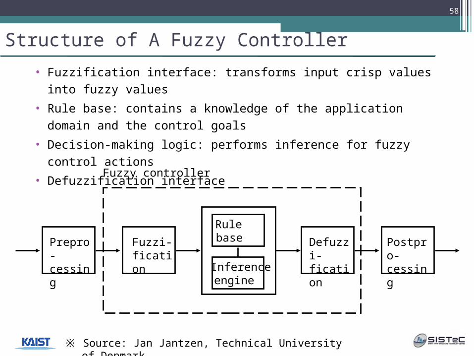
Structure of A Fuzzy Controller

• Fuzzification interface: transforms input crisp values into fuzzy values

• Rule base: contains a knowledge of the application domain and the control goals

• Decision-making logic: performs inference for fuzzy control actions

• Defuzzification interfaceFuzzy controller

Inferenceengine

Rulebase Defuzzi-

ficationPostpro-cessing

Fuzzi-fication

Prepro-cessing

58

※ Source: Jan Jantzen, Technical University of Denmark

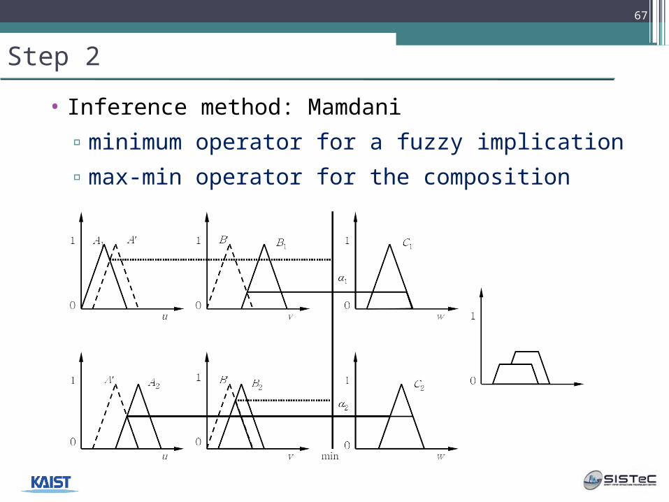
59

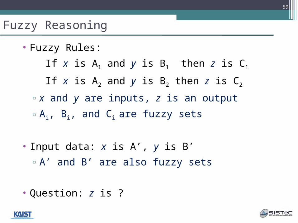
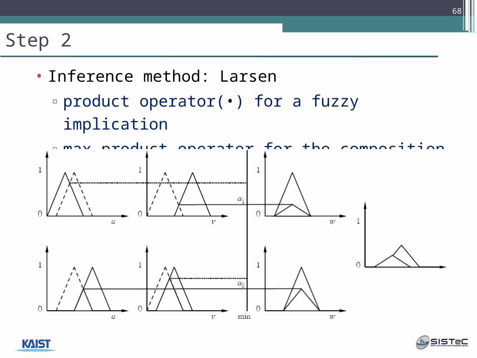
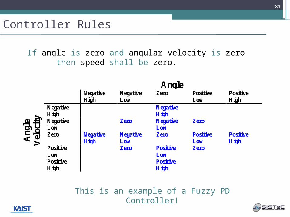
Fuzzy Reasoning

• Fuzzy Rules:

If x is A1 and y is B1 then z is C1

If x is A2 and y is B2 then z is C2

▫x and y are inputs, z is an output

▫Ai, Bi, and Ci are fuzzy sets

• Input data: x is A’, y is B’

▫A’ and B’ are also fuzzy sets

• Question: z is ?

60

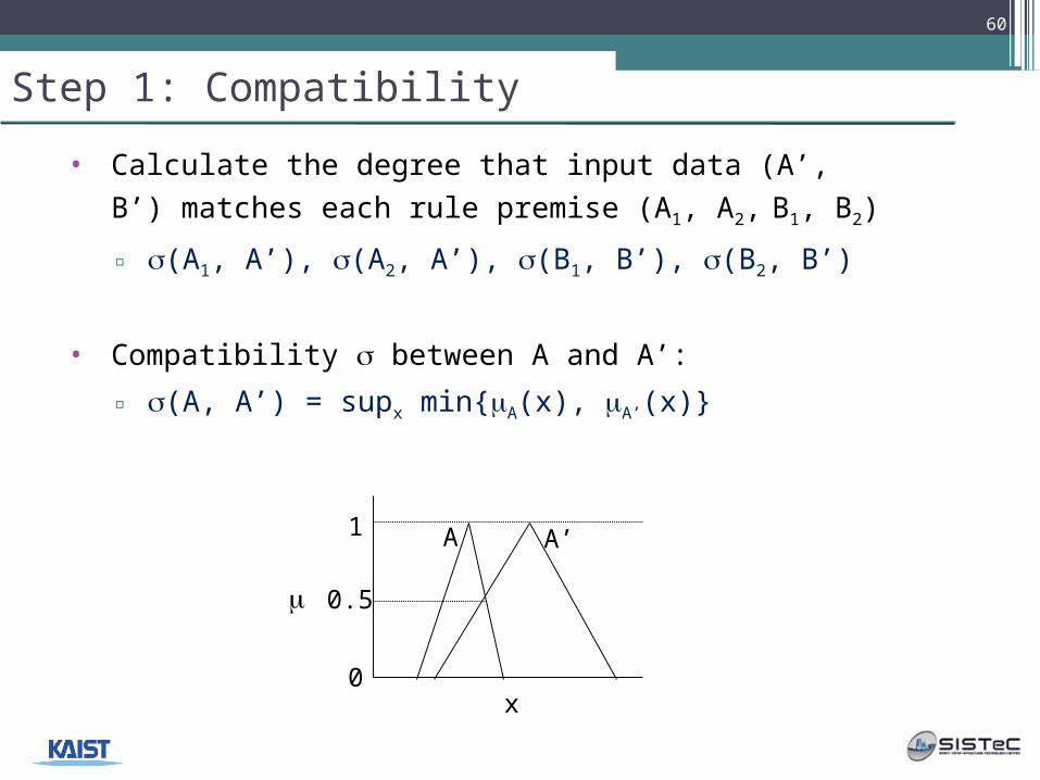
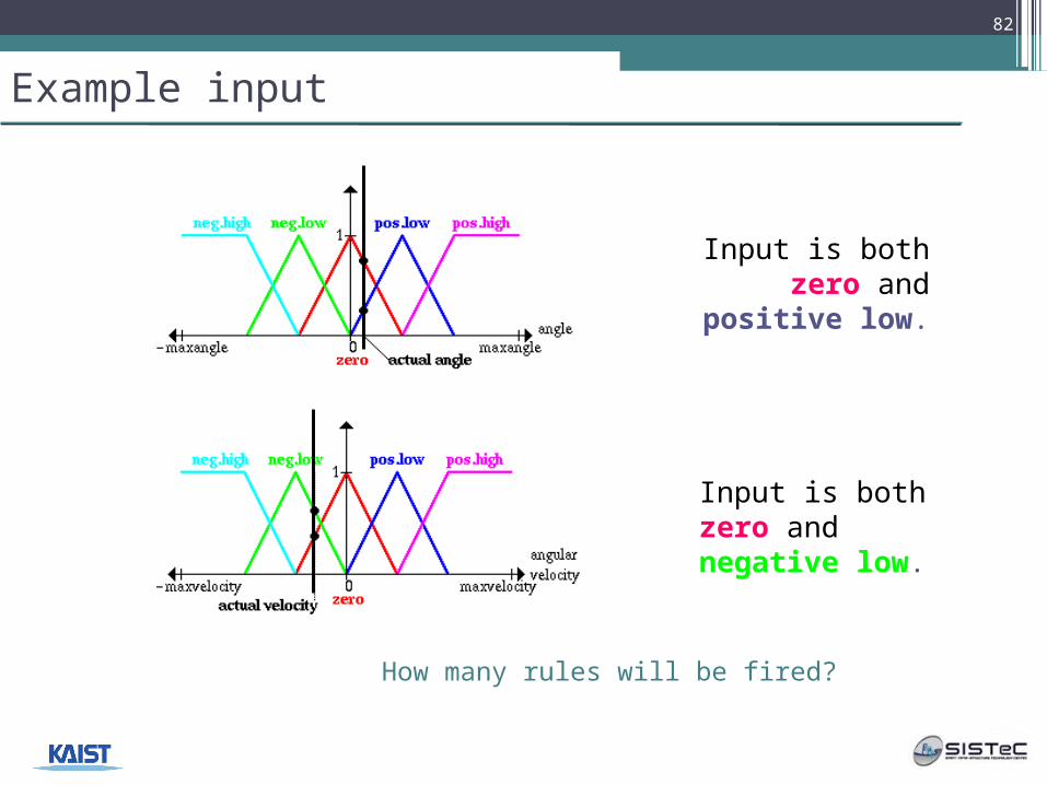
Step 1: Compatibility

• Calculate the degree that input data (A’, B’)

matches each rule premise (A1, A2, B1, B2)

▫ (A1, A’), (A2, A’), (B1, B’), (B2, B’)

• Compatibility between A and A’:

▫ (A, A’) = supx min{A(x), A’(x)}

x

0.5

1

A’

0

A

61

Step 2: Combine Compatibilities

• Combine the degree of matching for the inputs

▫ for “and”, usually take min

▫ for “or”, usually take max

▫ min{(A1, A’), (B1, B’)}

▫ min{(A2, A’), (B2, B’)}

x

0.5

1

A’

0y

0.3

1

B’

0

A B

0.3

62

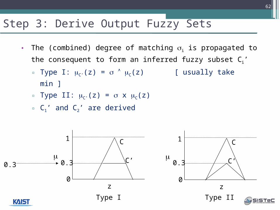
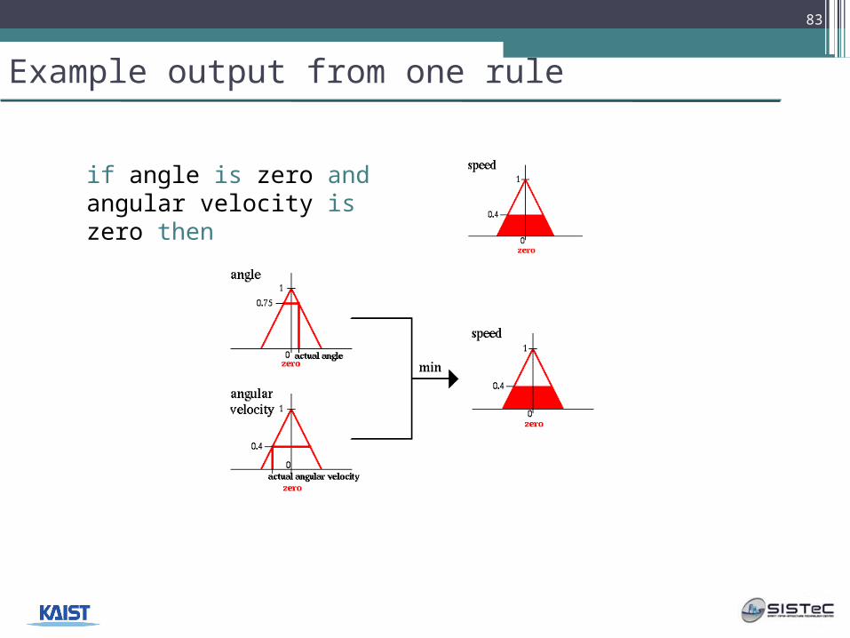
Step 3: Derive Output Fuzzy Sets

• The (combined) degree of matching i is propagated to

the consequent to form an inferred fuzzy subset Ci’

▫ Type I: C’(z) = C(z) [ usually take min ]

▫ Type II: C’(z) = x C(z)

▫ C1’ and C2’ are derived

z

1

C

0.3

0

C’

z

1

C

0.3

0

C’0.3

Type I Type II

63

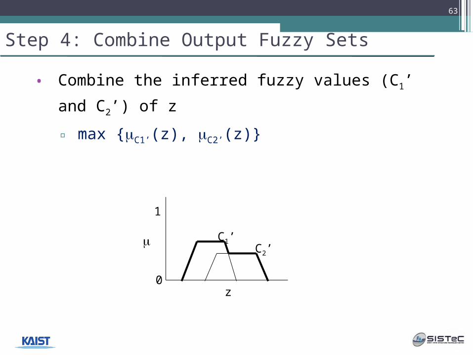
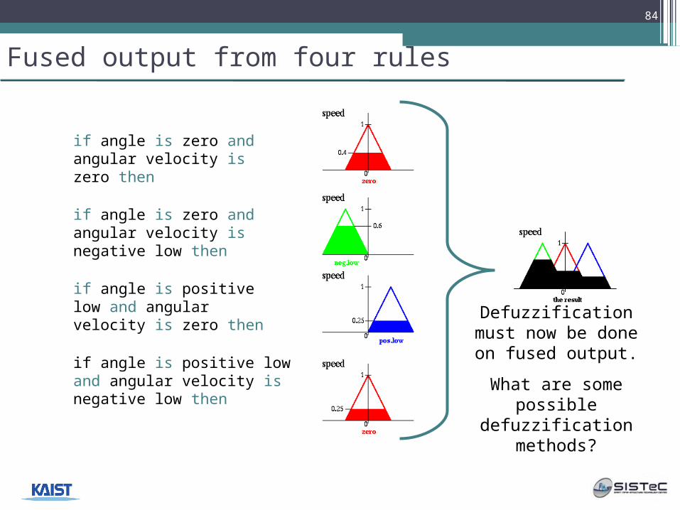
Step 4: Combine Output Fuzzy Sets

• Combine the inferred fuzzy values (C1’ and C2’)

of z

▫ max {C1’(z), C2’(z)}

z

1

0

C2’C1’

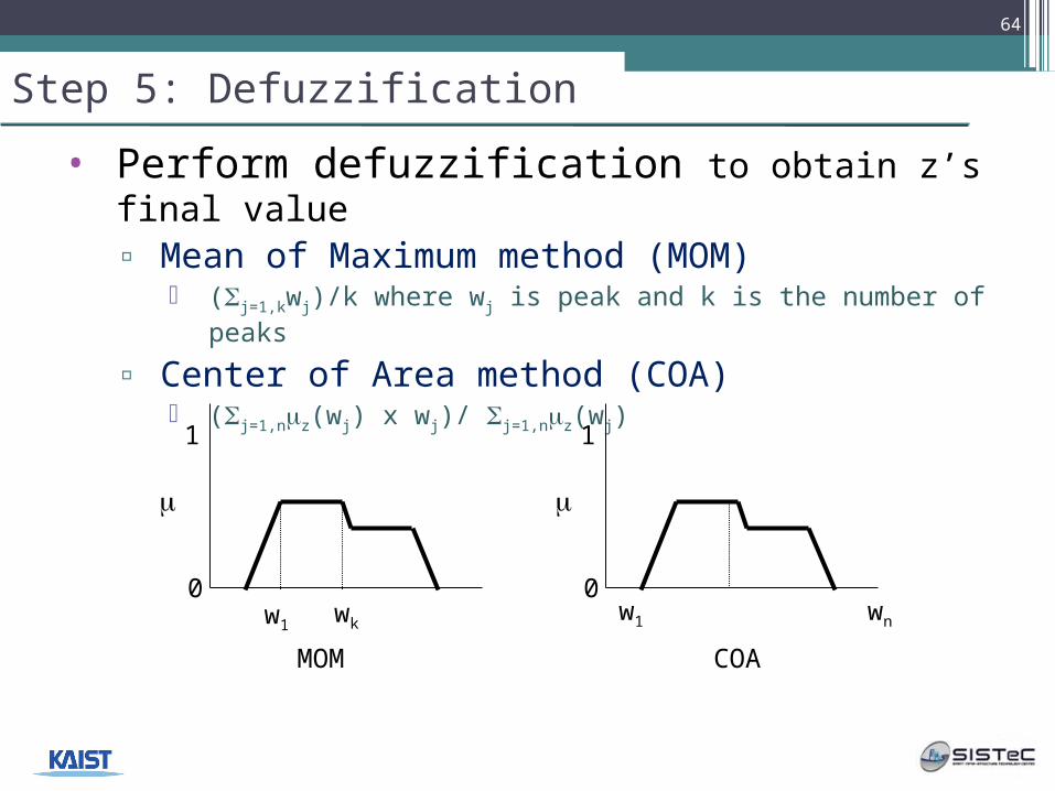
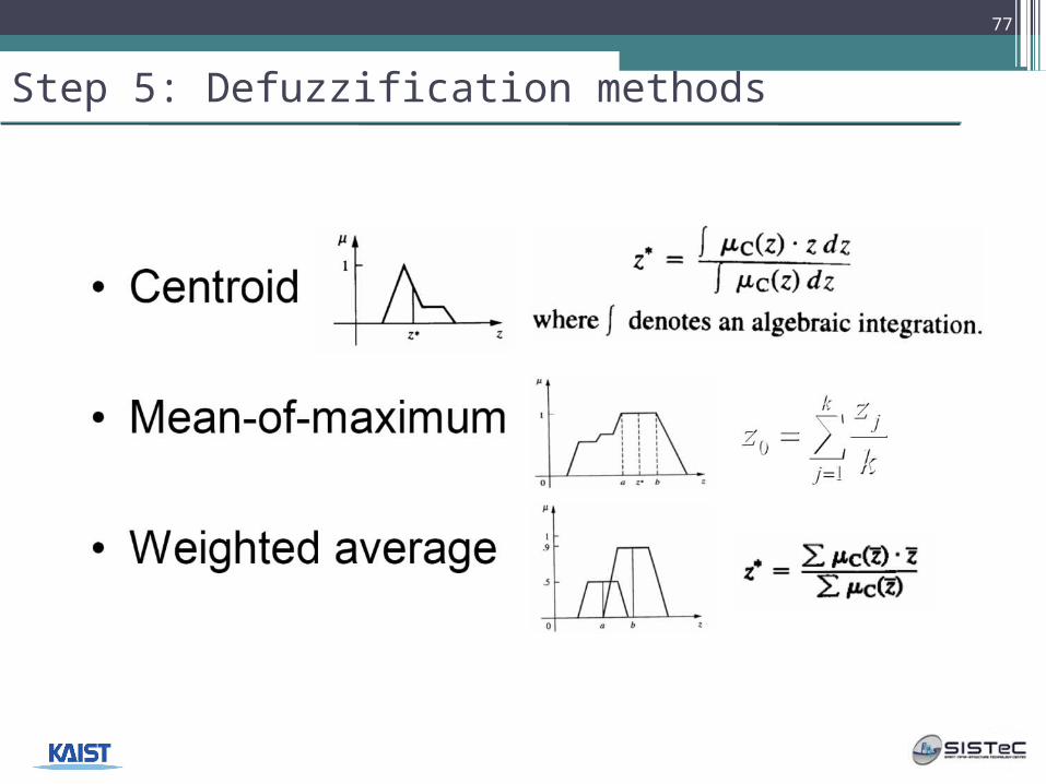
Step 5: Defuzzification

• Perform defuzzification to obtain z’s final value▫ Mean of Maximum method (MOM)

(j=1,kwj)/k where wj is peak and k is the number of peaks

▫ Center of Area method (COA) (j=1,nz(wj) x wj)/ j=1,nz(wj)

64

w1

1

0wk

MOM

1

0

COA

w1 wn

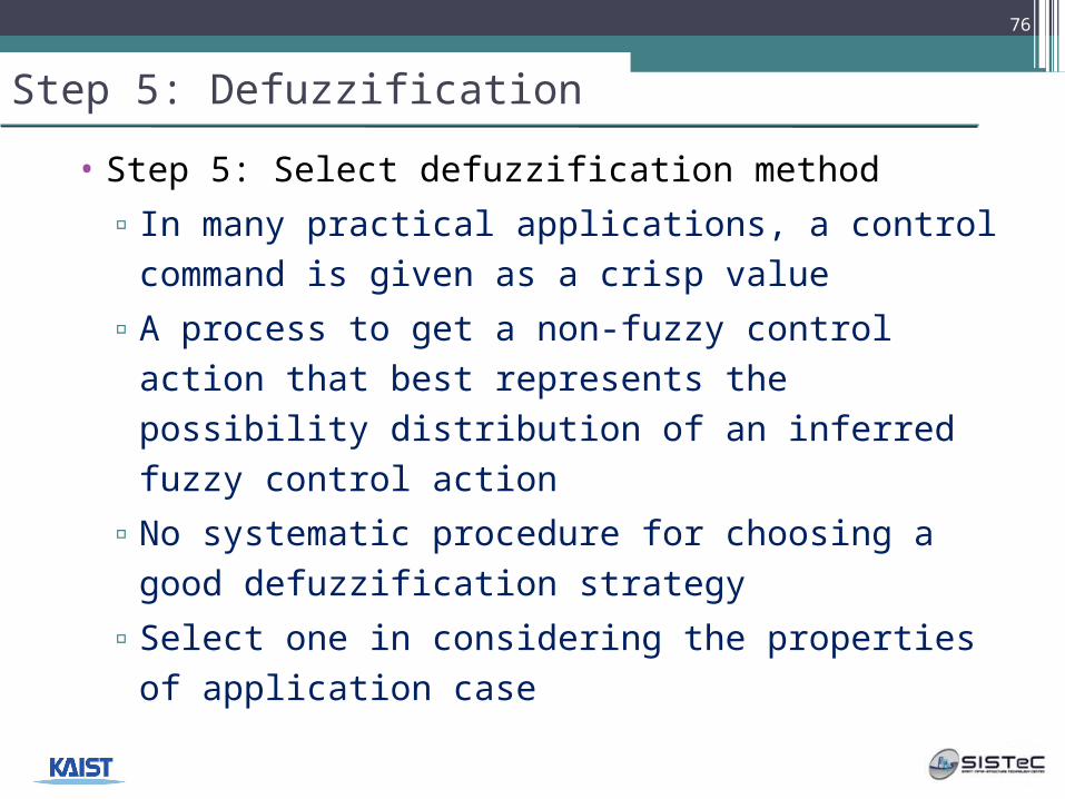
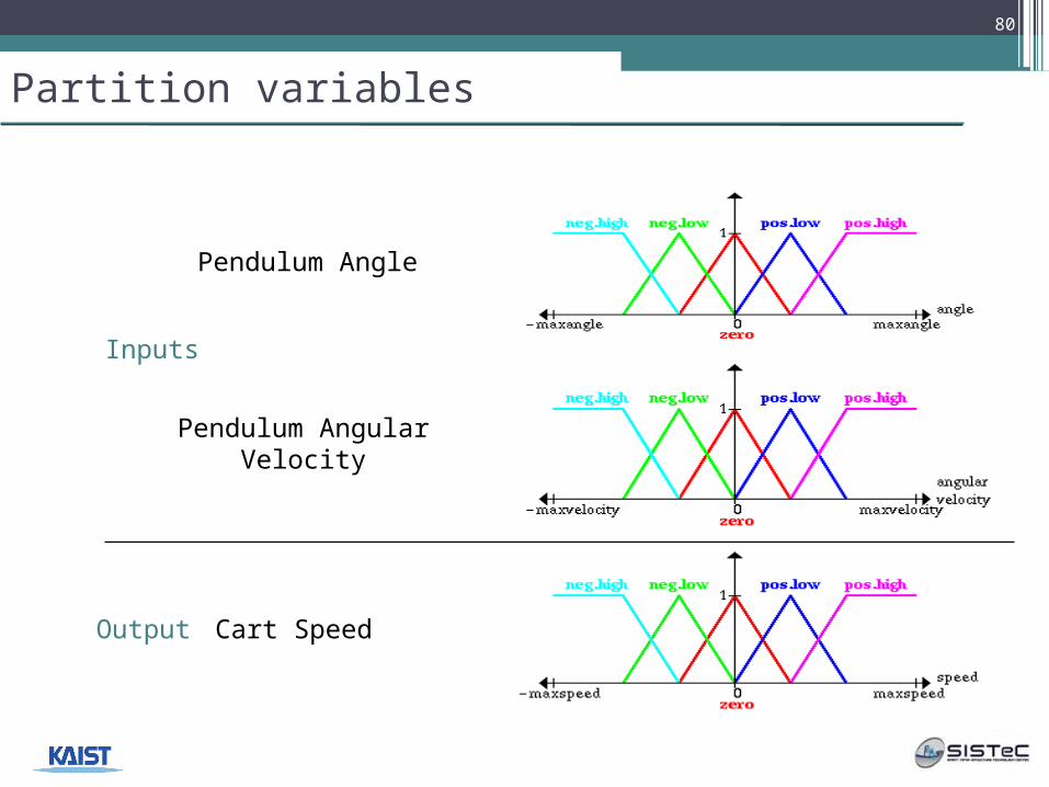
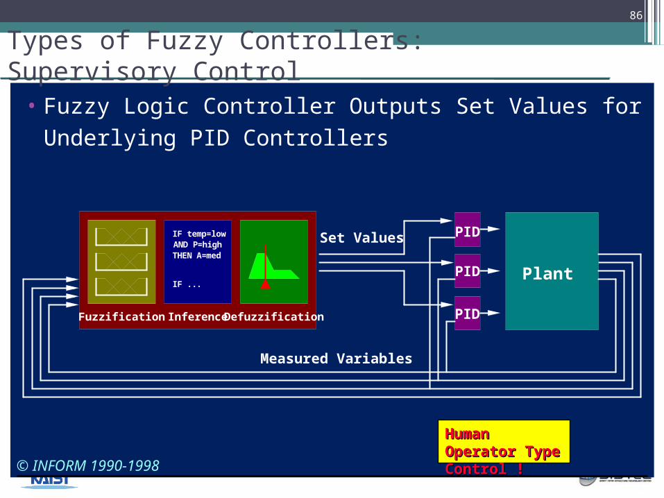
Fuzzy Controller Design: Step 1

• Step 1: Choice of state and control variables

• State variables

▫input variables of the fuzzy control system

▫state, state error, state error deviation, and state error integral are often used

• Control variables

▫output variables of the fuzzy control system

▫selection of the variables depends on expert knowledge on the process

65

※Source: http://if.kaist.ac.kr/lecture/cs670/textbook/

Step 2

• Step 2: Select inference method

▫Mamdani

▫Larsen

▫Tsukamoto

▫TSK (Takagi Sugeno Kang)

▫Other methods (such as SAM)

66

Step 2

• Inference method: Mamdani

▫minimum operator for a fuzzy implication

▫max-min operator for the composition

67

Step 2

• Inference method: Larsen

▫product operator(•) for a fuzzy implication

▫max-product operator for the composition

68

Step 2

• Inference method: TSK (Takagi-Sugeno-Kang)

69

Step 3

• Step 3: Fuzzification. Process of making a crisp quantity fuzzy

▫ If it is assumed that input data do not contain noise of vagueness, a fuzzy singleton can be used

▫ If the data are vague or perturbed by noise, they should be converted into a fuzzy number

70

Step 3

• Data base design

▫Discretization of the universe of discourse.

▫The scale mapping can be uniform, non-uniform, or both.

71

Example: A universe of discourse is discretized into 13levels (-6, -5, -4, … , 0, 1, … , 5, 6).

Step 4

• Step 4: Design the knowledge base.

• The knowledge base consists of two parts:

1. Data base. Partition of the variable spaces

2. Rule base. Fuzzy control rules.

72

Step 4: Data base design: Fuzzy partition

• 7 linguistic terms are often used▫ NB: negative big

▫ NM: negative medium

▫ NS: negative small

▫ ZE: zero

▫ PS: positive small

▫ PM: positive medium

▫ PB: positive big

• The number of fuzzy terms in the input space determines the maximum possible number of control rules.

73

Step 4: Rule base design

• Source of fuzzy control rules:

▫ Expert knowledge and control engineering knowledge

▫ Observation of operator’s actions

▫ Fuzzy model of the process: linguistic description of the dynamic properties

▫ Learning: learning from example or self-organizing learning

• State evaluation fuzzy rules

▫ state variables in the antecedent part, control variables in the consequent part.

74

Step 4: Rule base design

• A set of fuzzy rules

▫Ri: if x is Ai, and y is Bi then z is Ci, i = 1, 2, … , n

• Can be represented as a rule table

75

Step 5: Defuzzification

• Step 5: Select defuzzification method

▫In many practical applications, a control command is given as a crisp value

▫A process to get a non-fuzzy control action that best represents the possibility distribution of an inferred fuzzy control action

▫No systematic procedure for choosing a good defuzzification strategy

▫Select one in considering the properties of application case

76

Step 5: Defuzzification methods

77

Step 6

• Step 6: Test and tuning

▫Adjust data base

▫Adjust rule base

▫Try different inference methods

▫Try different defuzzification methods

78

Fuzzy Control Example: Inverted Pendulum

79

State variables

•Angle of the Pendulum

•Rate of change of the angle

•Position of the cart

Problem

Keep pendulum upright by moving cart left or right.

http://www.flll.uni-linz.ac.at/aboutus/whatisfuzzy/introduction.html

Partition variables

80

Cart Speed

Pendulum Angle

Pendulum AngularVelocity

Inputs

Output

Controller Rules

81

If angle is zero and angular velocity is zero then speed shall be zero.

Angle

Ang

le

Vel

ocit

y

Negative High

Negative Low

Zero Positive Low

Positive High

Negative High

Negative High

Negative Low

Zero Negative Low

Zero

Zero

Negative High

Negative Low

Zero Positive Low

Positive High

Positive Low

Zero Positive Low

Zero

Positive High

Positive High

This is an example of a Fuzzy PD Controller!

Example input

Input is both zero and

positive low.

Input is both zero and negative low.

How many rules will be fired?

82

Example output from one rule

83

if angle is zero and angular velocity is zero then

Fused output from four rules

84

if angle is zero and angular velocity is zero then

if angle is zero and angular velocity is negative low then

if angle is positive low and angular velocity is zero then

if angle is positive low and angular velocity is negative low then

Defuzzification must now be done on

fused output.

What are some possible

defuzzification methods?

• The Outputs of the Fuzzy Logic System Are the Command Variables of the Plant

Fuzzification Inference Defuzzification

IF temp=lowAND P=highTHEN A=med

IF ...

Variables

Measured Variables

Plant

Command

Fuzzy Rules Output Fuzzy Rules Output Absolute Values ! Absolute Values !

Types of Fuzzy Controllers: Direct Controller

85

© INFORM 1990-1998

• Fuzzy Logic Controller Outputs Set Values for Underlying PID Controllers

Fuzzification Inference Defuzzification

IF temp=lowAND P=highTHEN A=med

IF ...

Set Values

Measured Variables

Plant

PID

PID

PID

Human Operator Human Operator Type Control ! Type Control !

Types of Fuzzy Controllers: Supervisory Control

86

© INFORM 1990-1998

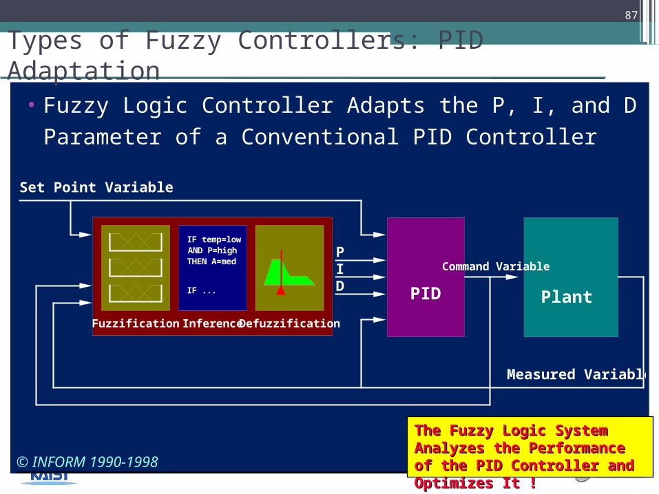
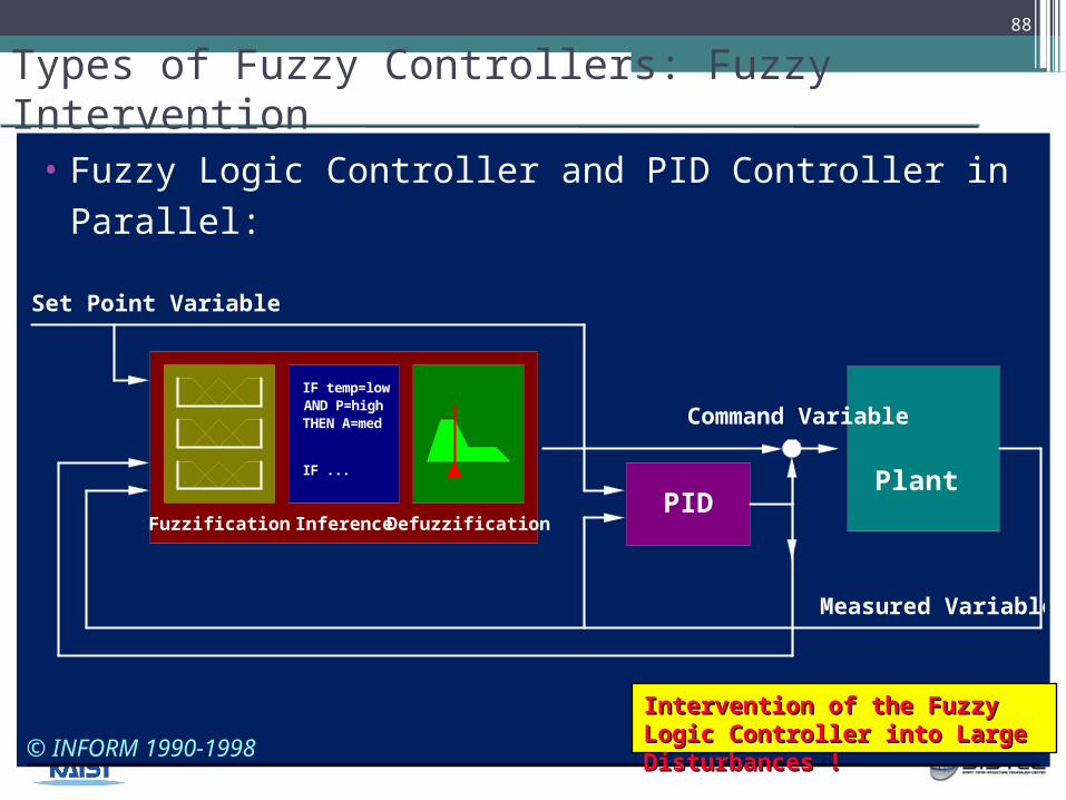
• Fuzzy Logic Controller Adapts the P, I, and D Parameter of a Conventional PID Controller

Fuzzification Inference Defuzzification

IF temp=lowAND P=highTHEN A=med

IF ...

P

Measured Variable

PlantPID

ID

Set Point Variable

Command Variable

The Fuzzy Logic System The Fuzzy Logic System Analyzes the Performance of the Analyzes the Performance of the PID Controller and Optimizes It !PID Controller and Optimizes It !

Types of Fuzzy Controllers: PID Adaptation

87

© INFORM 1990-1998

• Fuzzy Logic Controller and PID Controller in Parallel:

Fuzzification Inference Defuzzification

IF temp=lowAND P=highTHEN A=med

IF ...

Measured Variable

PlantPID

Set Point Variable

Command Variable

Intervention of the Fuzzy Logic Intervention of the Fuzzy Logic Controller into Large Disturbances !Controller into Large Disturbances !

Types of Fuzzy Controllers: Fuzzy Intervention

88

© INFORM 1990-1998

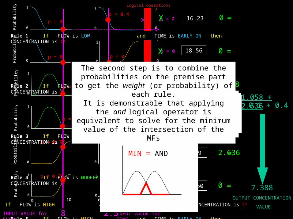
Rule 1 If FLOW is LOW and TIME is EARLY ON then CONCENTRATION is C1

Rule 2 If FLOW is LOW and TIME is LATER ON then CONCENTRATION is C2

Rule 3 If FLOW is MODERATE and TIME is EARLY ON then CONCENTRATION is C3

Rule 4 If FLOW is MODERATE and TIME is LATER ON then CONCENTRATION is C4

Rule 5 If FLOW is HIGH and TIME is EARLY ON then CONCENTRATION is C5

0

1

Pro

bab

ility

0

1

0

1

Pro

bab

ility

0

1

0

1

0

1

0

1

0

1

0

1

Pro

bab

ility

0

1

Pro

bab

ility

0

1

Pro

bab

ility

0

1

Pro

bab

ility

0 10 0 10Rule 6 If FLOW is HIGH and TIME is LATER ON then CONCENTRATION is C6

0

1

0

1

0

1

0

1

0

1

0

1

16.23

18.56

10.58

16.13

6.59

10.60

Logical operations

p = 0

p = 0

p= 0.1

p = 0

p= 0.4

p = 0

1.058 + 2.6360.1 + 0.4

7.388OUTPUT CONCENTRATION

VALUE

8 2.5INPUT VALUE for FLOW

p = 0

p = 0 p = 0

p = 0

p = 0

p = 0.4

p = 0.1

p = 0.1

p = 0.4

p = 0.75

p = 0.75

p = 0.4

INPUT VALUE for TIME

X =

X =

X =

X =

X =

X =

0

0

1.058

0

2.636

0

Given an input, the first step to solve the FIS is the fuzzyfication of inputs, i.e. to obtain the probability

of each linguistic value in each rule.

The six rules governing the Fuzzy Inference System are represented with a graphical representation of the

MFs that apply in each rule.

The last step is the defuzzyfication procedure, when the consequents are aggregated (weighted mean) to

obtain a crisp output

The third step is to calculate the consequent of each rule depending on their weight (or probability)

MIN = AND

The second step is to combine the probabilities on the premise part to get the weight (or probability) of

each rule.It is demonstrable that applying the and logical

operator is equivalent to solve for the minimum value of the intersection of the MFs

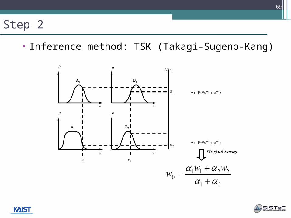
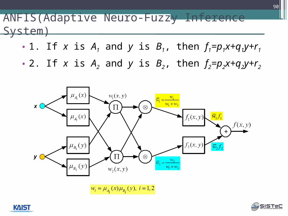
ANFIS(Adaptive Neuro-Fuzzy Inference System)

• 1. If x is A1 and y is B1, then f1=p1x+q1y+r1

• 2. If x is A2 and y is B2, then f2=p2x+q2y+r2

90

+

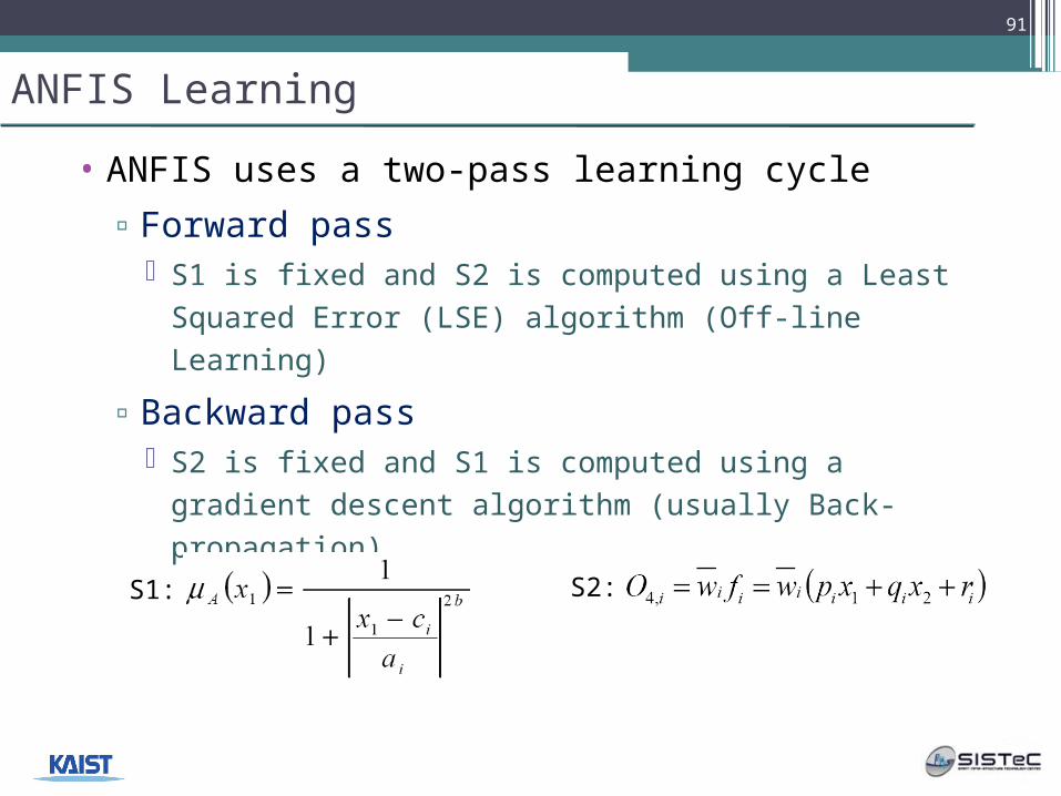
ANFIS Learning

• ANFIS uses a two-pass learning cycle

▫Forward pass S1 is fixed and S2 is computed using a Least Squared

Error (LSE) algorithm (Off-line Learning)

▫Backward pass S2 is fixed and S1 is computed using a gradient

descent algorithm (usually Back-propagation)

91

S1: S2:

92

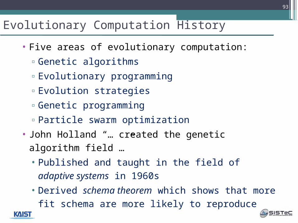
Evolutionary Computation History

• Five areas of evolutionary computation:

▫Genetic algorithms

▫Evolutionary programming

▫Evolution strategies

▫Genetic programming

▫Particle swarm optimization

• John Holland “… created the genetic algorithm field …”

• Published and taught in the field of adaptive systems in 1960s

• Derived schema theorem which shows that more fit schema are more likely to reproduce

93

Genetic Algorithms

• What are they?

▫GAs perform a random search of a defined N-dimensional solution space

▫GAs mimic processes in nature that led to evolution of higher organisms Natural selection (“survival of the fittest”) Reproduction

Crossover Mutation

▫GAs do not require any gradient information and therefore may be suitable for nonlinear problems

94

Genetic Algorithms

• Rely heavily on random processes

▫A random number generator will be called thousands of times during a simulation

• Searches are inherently computationally intensive

• Usually will find the global max/min within the specified search domain

95

General Procedure for Implementing a GA

1. Initialize population

2. Evaluate fitness of each member

3. Reproduce with fittest members

4. Introduce random crossover and/or mutations in new generation

5. Continue (2)-(3)-(4) until prespecified number of generations are complete

96

Encoding

• Population stored as coded “genes”

▫Binary Encoding Represents data as strings of binary numbers Useful for certain GA operations (e.g., crossover)

▫Real number encoding Represent data as arrays of real numbers Useful for engineering problems

97

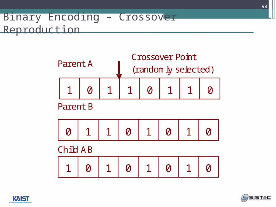
Binary Encoding – Crossover Reproduction

Parent A Parent B Child AB

Crossover Point (randomly selected)

1 0 1 1 0 1 1 0

0 1 1 0 1 0 1 0

1 0 1 0 1 0 1 0

98

Binary Encoding

• Mutation

▫Generate a random number for each “chromosome” (bit);

▫If the random number is greater than a “mutation threshold” selected before the simulation, then flip the bit

99

Real Number Encoding

• Genes stored as arrays of real numbers

• Parents selected by sorting population best to

worst and taking the top “Nbest” for random

reproduction

100

Real Number Encoding

• Reproduction

▫Weighted average of the parent arrays:Ci = wAi + (1-w)*Bi

where w is a random number 0 ≤ w ≤ 1

▫If sequence of arrays are relevant, use a crosover-like scheme on the children

101

Real Number Encoding

• Mutation

▫If mutation threshold is passed, replace the entire array with a randomly generated one

▫Introduces large changes into population

102

Real Number Encoding

• Creep

▫If a “creep threshold” is passed, scale the member of the population with

Ci = ( 1 + w )*Ciwhere w is a random number in the range 0 ≤ w ≤ wmax. Both the creep threshold and wmax must be specified before the simulation begins

▫Introduces small scale changes into population

103

•Matlab Neural Networks Toolbox•Matlab Fuzzy Logic Toolbox•Neuro-Fuzzy Controller: ANFIS•Simple GA Example•References

104

MATLAB® Toolbox – Neural Networks

• Facilitates easy construction, training and use of NNs

▫ Concurrent and recurrent networks

▫ Linear, tansig, and logsig activation functions

▫ Variety of training algorithms Backpropagation

Descent methods (CG, Steepest Descent…)

• nntool: invokes NN GUI

105

Model Reference Neuro-Control: mrefrobotarm

106

MATLAB® Toolbox – Fuzzy Logic

• fuzzy [fisname] : invokes FIS editor or loads ‘fisname’ FIS

• readfis / writefis : loads / saves “*.fis” file

• anfisedit : invokes ANFIS editor

• fuzblock : SIMULINK fuzzy controller block

• Example

▫ sltank

▫ slcp

107

FIS editor: fuzzy

108

ANFIS editor: anfisedit

109

ANFIS: Initializing

• Initialize the fuzzy system

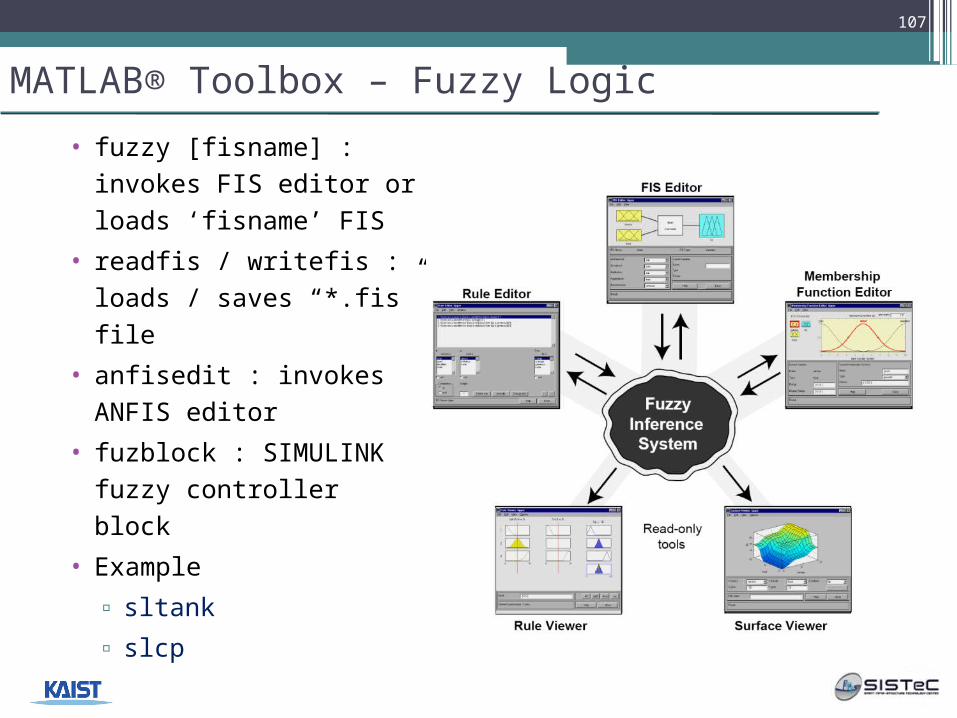
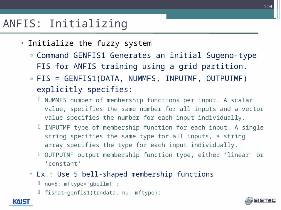
▫ Command GENFIS1 Generates an initial Sugeno-type FIS for ANFIS training using a grid partition.

▫ FIS = GENFIS1(DATA, NUMMFS, INPUTMF, OUTPUTMF) explicitly specifies: NUMMFS number of membership functions per input. A scalar

value, specifies the same number for all inputs and a vector value specifies the number for each input individually.

INPUTMF type of membership function for each input. A single string specifies the same type for all inputs, a string array specifies the type for each input individually.

OUTPUTMF output membership function type, either 'linear' or 'constant‘

▫ Ex.: Use 5 bell-shaped membership functions nu=5; mftype='gbellmf';

fismat=genfis1(trndata, nu, mftype);

110

ANFIS: Learning

• [FIS,ERROR,STEPSIZE] = ANFIS(TRNDATA,INITFIS,TRNOPT,DISPOPT,[],OPTMETHOD)

▫ uses the vector TRNOPT to specify training options: TRNOPT(1): training epoch number (default: 10)

TRNOPT(2): training error goal (default: 0)

TRNOPT(3): initial step size (default: 0.01)

TRNOPT(4): step size decrease rate (default: 0.9)

TRNOPT(5): step size increase rate (default: 1.1)

▫ OPTMETHOD selects the optimization method used in training. Select 1 to use the default hybrid method, which combines least squares

estimation with backpropagation.

Select 0 to use the backpropagation method.

▫ Ex: numep=100;

[parab,trnerr,ss,parabcheck,chkerr] = anfis(trndata,fismat,numep,[],chkdata);

111

ANFIS: Evaluating

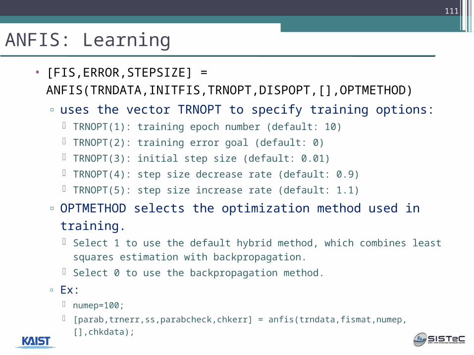
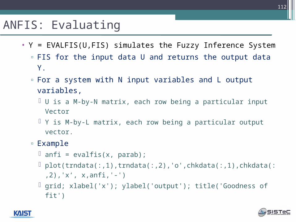
• Y = EVALFIS(U,FIS) simulates the Fuzzy Inference System

▫ FIS for the input data U and returns the output data Y.

▫ For a system with N input variables and L output variables, U is a M-by-N matrix, each row being a particular input

Vector Y is M-by-L matrix, each row being a particular output

vector.

▫ Example anfi = evalfis(x, parab); plot(trndata(:,1),trndata(:,2),'o',chkdata(:,1),chkdata(:,2),'x‘,

x,anfi,'-') grid; xlabel('x'); ylabel('output'); title('Goodness of fit')

112

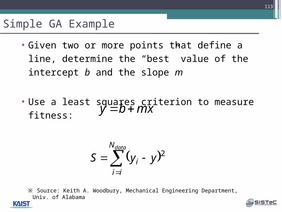
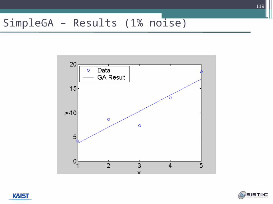
Simple GA Example

• Given two or more points that define a line, determine the “best” value of the intercept b and the slope m

• Use a least squares criterion to measure fitness:

dataN

iii yyS 2

mxby

113

※ Source: Keith A. Woodbury, Mechanical Engineering Department, Univ. of Alabama

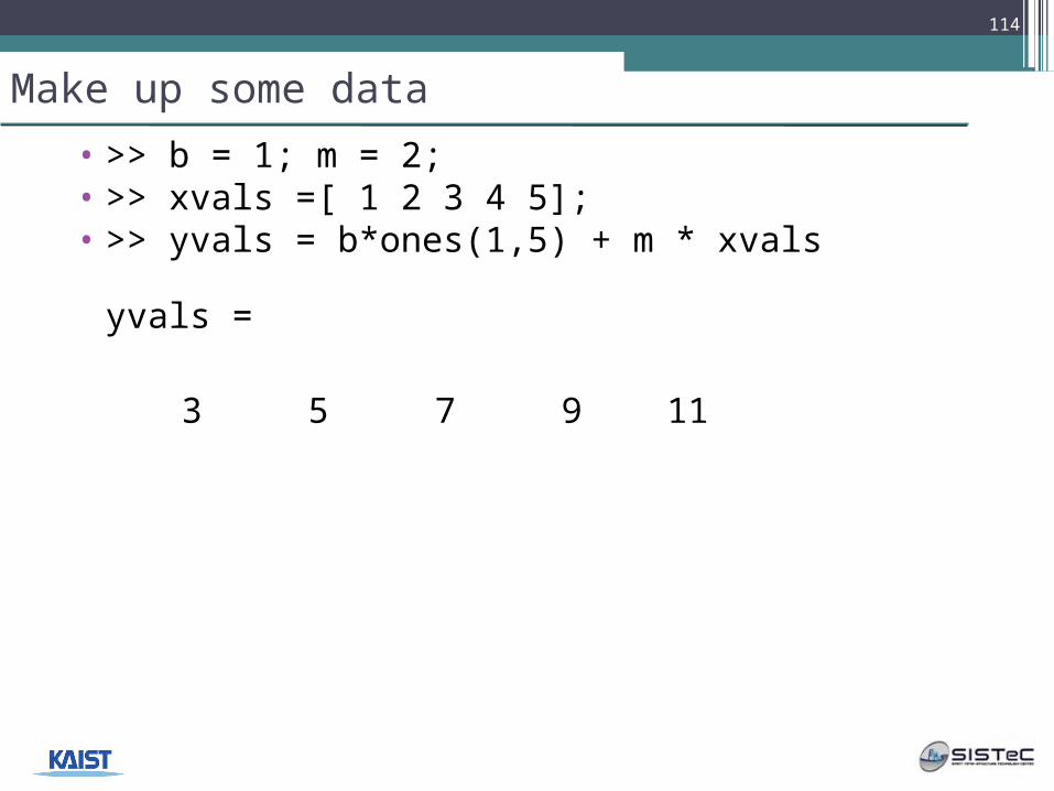
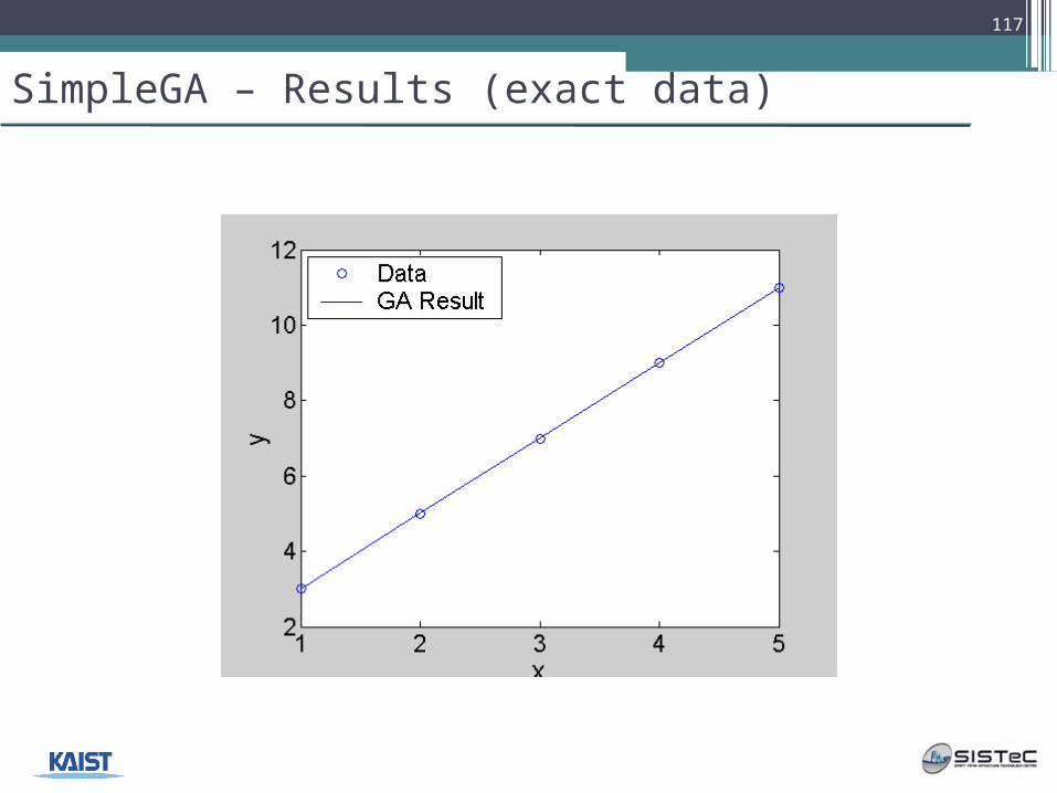
Make up some data

• >> b = 1; m = 2;• >> xvals =[ 1 2 3 4 5];• >> yvals = b*ones(1,5) + m * xvals

yvals =

3 5 7 9 11

114

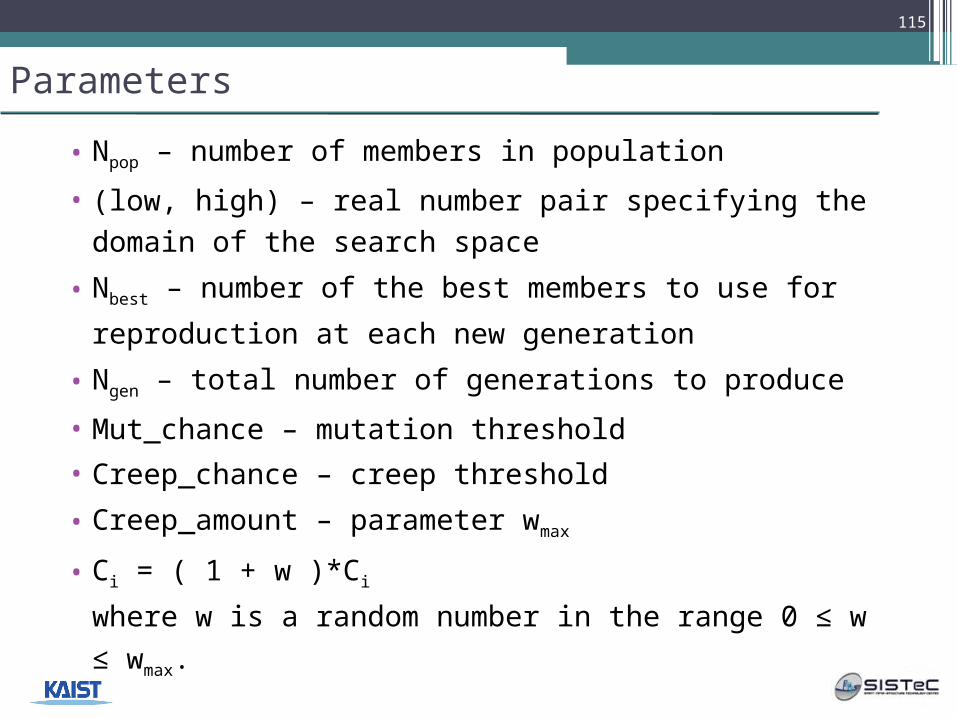
Parameters

• Npop – number of members in population

• (low, high) – real number pair specifying the domain of the search space

• Nbest – number of the best members to use for

reproduction at each new generation

• Ngen – total number of generations to produce

• Mut_chance – mutation threshold

• Creep_chance – creep threshold

• Creep_amount – parameter wmax

• Ci = ( 1 + w )*Ci

where w is a random number in the range 0 ≤ w ≤

wmax.

115

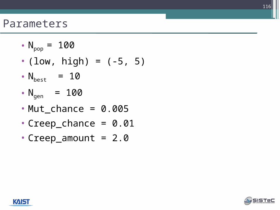
Parameters

• Npop = 100

• (low, high) = (-5, 5)

• Nbest = 10

• Ngen = 100

• Mut_chance = 0.005

• Creep_chance = 0.01

• Creep_amount = 2.0

116

SimpleGA – Results (exact data)

117

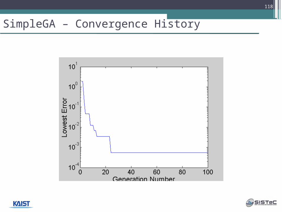
SimpleGA – Convergence History

118

SimpleGA – Results (1% noise)

119

SimpleGA – Results (10% noise)

120

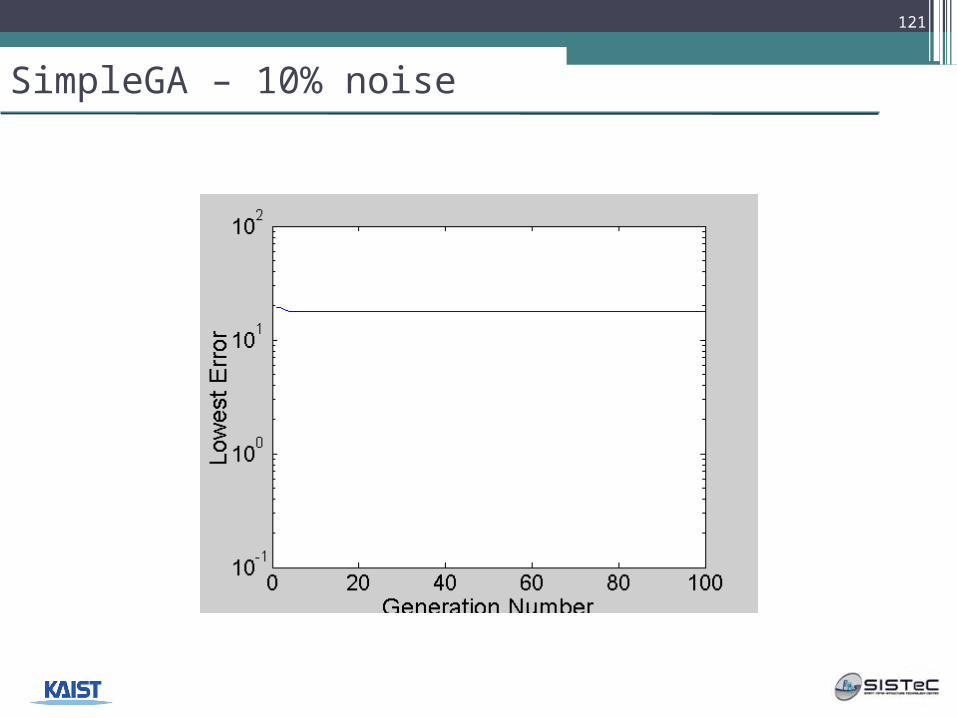
SimpleGA – 10% noise

121

References

• Computational Intelligence: Concepts to Implementations (Russell Eberhart and Yuhui Shi, Publisher: Morgan Kaufmann, 2007)

• Soft Computing and Intelligent Systems Design: Theory, Tools and Applications (Fakhreddine O. Karray and Clarence De Silva, Addision-Wesley, 2004)

• Yaxi Shen and Abdollah Homaifar, “Vibration Control of Flexible Structures with PZT Sensors and Actuators,” Journal of Vibration and Control, vol. 7, no. 3, pp.417-451, 2001.

• For more on lecture material, please visit http://web.kaist.ac.kr/~ceerobot and look at BBS.

122