ACTIVE VIBRATION CONTROL FOR STRUCTURE HAVING...

International Conference on Earthquake Engineering and Disaster Mitigation, Jakarta, April 14-15, 2008

ACTIVE VIBRATION CONTROL FOR STRUCTURE HAVING NON-LINEAR BEHAVIOR UNDER EARTHQUAKE EXCITATION

Herlien D. Setio1 and Sangriyadi Setio2

1 Department of Civil Engineering, Institut Teknologi Bandung

2 Department of Mechanical Engineering, Institut Teknologi Bandung

ABSTRACT: A study on actively controlled responses of non-linear system using Artificial Neural Network (ANN) is presented in this paper. The capability to learn, the ability to generalize to new inputs and the ability to perform fast computations are the major advantages in application of neural network. The responses of the non-linear system, which is governed by Duffing’s equation and driven by a harmonic force, are determined through the utilization of equivalent linearization method. The active force at any step of amplitude is determined by using an optimal control algorithm which is then used as input data for neural network training. The advantage of utilizing the neural network as a neuro-controller is that it can considerably reduce computing steps and time.

1. INTRODUCTION

It is common knowledge that buildings and structures must withstand ever-changing environmental loads, such as wind, earthquakes and waves, over the span of their useful lives. Yet, until very recently, buildings, bridges, and other constructed facilities have been built as passive structures that rely on their mass and solidity to resist outside forces, while being incapable of adapting to the dynamics of an ever-changing environment.

In order to design adaptive structures, the concept of structural control was introduced. The control concept has been used for a long time for airplanes, ships, and space structures. However, its application to civil structures has only recently been taken into consideration. Structural control involves basically the regulating of structural characteristics as to ensure desirable response of the structure under the effect of its loading. These mechanisms provide in general a system of auxiliary forces, the so-called control forces. These forces are designed so that they regulate continuously the structural response.

Using the conventional control algorithm in order to get the control forces required to control the structure, one must go through several complicated steps that usually takes a long computational time. By using the block of neural network for computing the control forces instead of using the conventional control algorithm, the computation time can be reduced significantly.

Active control of linear structures is well developed and is a powerful technique to control vibrations in civil engineering structures against natural dynamic loads. Unfortunately most of the civil engineering structures exhibit non-linearity in certain local regions or possibly in the whole of the structure. The non-linear systems of routine engineering practice, particularly those subjected to dynamic loads, have continued to be solved by linear methods. For some types of non-linearity, a linear model for the structure is no longer appropriate in the analysis of real structures.

It is possible to obtain modal properties with sufficient accuracy at low level of excitation, but it may be completely distorted at higher levels. In many theoretical studies, it has been found that the period of vibration decreases rapidly with increasing amplitude of vibration. In this study a cubic hardening non-linearity in the form of Duffing’s equation is used as non-linear system model.

The study presents a simple and rapid solution, in regard to computational cost and the mathematical complexities of active control of structures having non-linear stiffness. The solution is based on the linear modal analysis. At any step of amplitude, the non-linear mode is used for transforming the set of n coupled equations from a physical base motion of an n degree-of-freedom system into a set of n uncoupled equations in a modal base system and then the active

Back to Table of Contents 697


force is determined as a function of modal amplitude by using an optimal control algorithm. The control force and the measured acceleration response of the structure are feed to the artificial neural network system as a set of training data. The reliability of the active control for non-linear systems is tested by using various sinusoidal excitation and Flores earthquake base acceleration.

2. VIBRATION CONTROLLER

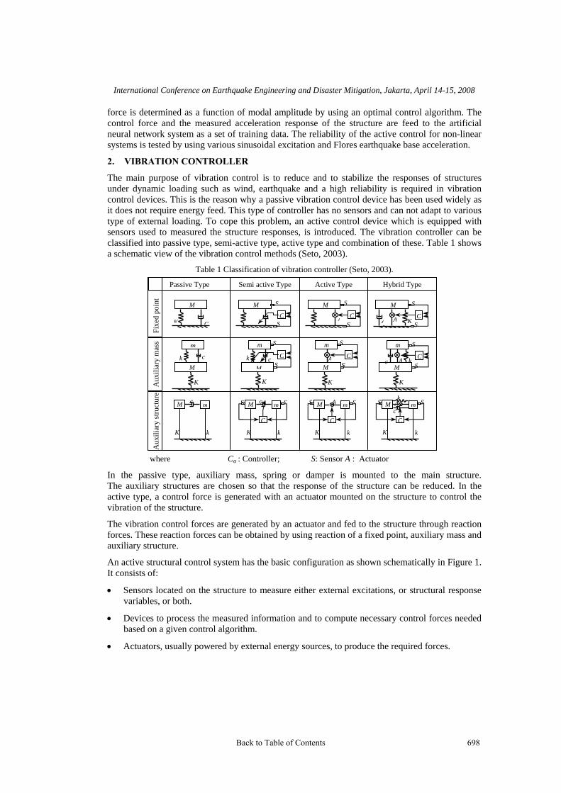
The main purpose of vibration control is to reduce and to stabilize the responses of structures under dynamic loading such as wind, earthquake and a high reliability is required in vibration control devices. This is the reason why a passive vibration control device has been used widely as it does not require energy feed. This type of controller has no sensors and can not adapt to various type of external loading. To cope this problem, an active control device which is equipped with sensors used to measured the structure responses, is introduced. The vibration controller can be classified into passive type, semi-active type, active type and combination of these. Table 1 shows a schematic view of the vibration control methods (Seto, 2003).

Table 1 Classification of vibration controller (Seto, 2003).

where Co : Controller; S: Sensor A : Actuator

In the passive type, auxiliary mass, spring or damper is mounted to the main structure. The auxiliary structures are chosen so that the response of the structure can be reduced. In the active type, a control force is generated with an actuator mounted on the structure to control the vibration of the structure.

The vibration control forces are generated by an actuator and fed to the structure through reaction forces. These reaction forces can be obtained by using reaction of a fixed point, auxiliary mass and auxiliary structure.

An active structural control system has the basic configuration as shown schematically in Figure 1. It consists of:

• Sensors located on the structure to measure either external excitations, or structural response variables, or both.

• Devices to process the measured information and to compute necessary control forces needed based on a given control algorithm.

• Actuators, usually powered by external energy sources, to produce the required forces.

M

C

S

S

MC

S

SA

M

CK

S

S AC

M

K C

M

K

mk c C

SM

K

m

k c

S

CSM

K

m S

AM

m

A

K

C

S

S k c

M

K k

mc M

K k

m S

C

S c M

K k

m S

C

S A M

K k

m S

C

S Ac

k

Aux

iliar

y st

ruct

ure

Aux

iliar

y m

ass

Passive Type Semi active Type Active Type

Fix

ed p

oint

Hybrid Type



Figure 1 Configuration of structural control system.

3. NON-LINEAR MODAL ANALYSIS

Consider a non-linear n-degree-of freedom system subjected to a harmonic excitation of frequencyΩ. The second order differential equation corresponding to the motion of this system can be expressed by

( ) tf Ω=+++ cos, PXXKXXCXM &&&& (1)

M, C, K, f( X& ,X) and P are the mass matrix, the damping matrix, the stiffness matrix, the vector or non-linear force which depends on the spatial displacements X and their derivatives, and the vector of the amplitude harmonic force, respectively.

3.1 Non-Linear Frequency and Mode

The principal approach of the method is the assumption that the mode of vibration in resonance conditions is assumed to be the same as the normal mode of the corresponding non-linear system and that all the non-resonant co-ordinates can be neglected except the single resonant coordinate. The stationary solution of the multi-degree-of-freedom system of Eq. (1) is reduced to single-degree-of-freedom system described by the single resonant normal co-ordinates at Ω = Ωj. Thus the stationary solution of the autonomous conservative system of Eq. (1) in the resonance condition can be approached as

tqt jjj Ωφ= sin)(X (2)

Here qj is the modal amplitude, jφ and Ωj are the unknown non-linear mode shape and the unknown non-linear resonance frequency of mode j.

There exist many numerical procedures for solving non-linear problems. The Newton-Raphson procedures are used for this study (Setio et al., 1992).

The unknown non-linear parameters can be obtained by inserting Eq. (2) into the autonomous conservative system of Eq. (1) and neglecting all the higher harmonic terms; one obtains

}]{[}){]([ jjjjq φλ=φ MD , where )()]([ jnlj qq KKD += , 2jΩ=λ (3, 4)

)( jnl qK is the non-linear stiffness matrix which depends on the modal amplitude qj .

In accordance with the Newton-Raphson procedure, the non-linear Eq. (3) can be rewritten in the form

( )[ ] ( )jjjjjnl gq φλ=φλ−+ ,MKK (5)

The non-linear frequencies and modes of the system are obtained as a function of modal amplitude qj by increasing the modal amplitude progressively:

EXTERNAL FORCES

STRUCTURAL RESPONSES STRUCTURE

CONTROL FORCES

ACTUATORS

SENSORS SENSORS

CALCULATION OF CONTROL FORCES



( ) ( ) jjjjjj qq φ=φλ=ω ,2 (6, 7)

( )jj qφ and ( )jj qω are the non-linear normal mode and natural frequency, respectively.

This algorithm should be rapidly converging for this iterative procedure, based upon the previous values for each given modal amplitude.

3.2 Equivalent Linearization Method

The principal approach of the method is the replacement of the non-linear differential equation by a linear equation in such a way that an average of the difference between the two systems is minimized.

Consider the non-linear second order differential equation of motion (1). The equivalent linear system may be expressed in the form

tΩ=++++ cos'' PXKXCKXXCXM &&&& (8)

C’ and K’ are the equivalent damping matrix and the equivalent stiffness matrix, respectively. The matrices C’ and K’ are determined by minimizing the difference ε between the non-linear system (1) and the equivalent linear system (8) for every x(t).

( ) XK'XC'X,Xε −−= &&f (9)

The minimization of ε is performed according to the criterion

=ε=εε ∫ dtT

ET

0

21)'( minimum, T = ωπ2 (10)

The necessary conditions for the minimization specified by eq. (10) are

0)'(

ijcE

′δδ εε

0)'(=

′δδ

ijkE εε

(11, 12)

where ijc′ and ijk ′ are the elements of the matrices C’ and K’, respectively. The equivalent linear terms can be constructed according to Eqs. (10), (11) and (12).

By assuming a periodic solution, the general solution of Eq. (8) can be approximated by Fourier series which are truncated to a single harmonic function

jjjjj qtttx )cossin()( ImRe Ωφ+Ωφ= (13)

jReφ and jImφ are the real and the imaginary parts of the non-linear complex mode.

4. STATE EQUATION AND CONTROL STRATEGY

4.1 Active Control

For any step of amplitude the equivalent state space equation of a non-linear n-degree-of-freedom system subjected to a dynamic excitation p(t) can be expressed by:

( ) ( ) ( ) ( )tpttt WBUAZZ ++=& , ( ) 00 ZZ =t (14)

with

⎥⎦

⎤⎢⎣

⎡=

)()(

)(tt

tXX

Z &, ⎥

⎦

⎤⎢⎣

⎡−−

= −− CMKMI

A 11 )(~jq

O, ⎥

⎦

⎤⎢⎣

⎡= − HM

B 1O , ⎥

⎦

⎤⎢⎣

⎡−

= − EMW 1

O



)()(~jnlj qq KKK += , Z(t) is the 2n state vector of displacements and velocities, A is the 2n x 2n

matrix of structural parameters, B is the 2n x m matrix specifying the location of the control forces, U(t) is the m vector of control forces, W is the 2n x 1 matrix specifying external loading location matrix. Optimal control of this structure can be determined by minimizing quadratic performance

( ) ( ) ( )[ ] tttttJft

d)(0

TT∫ += URUZQZ (15)

Q is a 2n x 2n symmetrical semi definite weighting matrix, R is an m x m symmetrical positive weighting matrix and tf is a time chosen to be longer than earthquake excitation. The determination of the Q and R is discussed by Soong et al. (1988).

The optimal control law is given by:

( ) ( ) ( )ttt T ZPBRZGU 121 −−== (16)

The problem of optimal control is to determine a gain vector G in such a way that a performance index J is minimized subject to the constraining Eq. (14). The state vector Z(t) is accessible through measurement.

The 2n x 2n symmetrical matrix P is determined by solving the following Riccati equation:

02121 =++− − QPAPBPBRPA TT (17)

Inserting Eq. (16) into Eq. (14), the state space Eq. (8) becomes:

( ) ( ) ( )tftt WZBGAZ ++= )(& (18)

The state space Eq. (18) shows that the structural parameters are changed from open-loop system A in Eq. (14) to closed-loop system A+BG.

4.2 Artificial Neural Network

An artificial neural network is a system with inputs and outputs, composed of a number of similar processing units (Setio et al., 1997b; Setio and Setio, 2003). These processing units operate in parallel and are arranged in a pattern. The units are connected to each other by adjustable weights as shown in Figure 2. Changing the weights will change the input-output behavior of the network, and weights are chosen in such a way as to achieve the desired input-output relationship. To achieve this goal, systematic ways of adjusting the weights have to be developed, which are called learning algorithms. The accuracy of the network depends on the number of neural in the layer. A neural network is characterized by the processing units, the network topology and the learning algorithm.

The selection of a neural number in the network layer is largely based on experience. The weighting constants are determined randomly. Through the learning process, those values will change in such a way so that in the end, the whole neural network will be able to give the expected output.

Figure 2 Architecture of artificial neural network.

j

Input x Output g

Wkj Wji

Output Layer

Hidden Layers Input Layer

k

i



4.3 Neural Control Force

Consider Z(t) is the state vector of the vector of displacement X(t) and vector of velocity )(tX& of the structure. The control force obtained by optimal control procedure is G(Z(t)). Inputs to the neural network are the acceleration measurements )(tX&& and the network output G( )(tX&& ) is the control force G(Z(t)). The neural network procedure consists of two steps, the learning step and the validation step. If the learning was successful the network should produce an output sequence very close to the actual system output.

5. NUMERICAL EXAMPLE

A discrete model of two-degree-of freedom system with a local non-linearity was chosen as an example to illustrate the advantage and the accuracy of the methods. A mass-spring system is depicted in Figure 3, where a cubic non-linear spring and a single harmonic excitation of frequency Ω are introduced at mass 1.

Figure 3 Model of non-linear two-degree-of-freedom system. m1=1 kg, m2=1.5 kg, k1=k2=1 N/m, c1=c2= 0.01

Ns/m, α1=0.001 N/m3.

The non-linear natural frequencies ω1 and ω2 as function of modal amplitude, shown in Figures 4, are calculated by the non-linear mode method of Eq. (6).

Figure 4 The non-linear natural frequencies as a function of modal amplitude q.

Figure 5 shows the frequency responses of the structure for three different amplitude forces. Some aspects of the non-linear phenomenon can be seen, such as jump phenomena and the dependence of the resonance frequency on the amplitude of vibration.

The active force of non-linear system as a function of amplitude is determined by using sinusoidal excitation of various amplitudes and frequencies. The control force and the acceleration response of the non-linear structure are feed to the artificial neural network system as a set of training data. A three layer neural network has been used for the neural controller. The input layer consists of 4 neurons with tansigmoid and purelin activation functions, the hidden layer has 30 neurons and the output layer has only one neuron that represents the control force.

The performance of the trained neural controller was tested through several numerical simulation. Figures 6a-b show the comparison between the uncontrolled and controlled structure responses of the non-linear structure determined from the optimal control and from the neural controller (ANN). The comparison is made in the case of the non-linear model as shown in Figure 3 which was subjected to sinusoidal excitation of amplitude F1=0.08 N, frequencies Ω=0.4 and Ω=0.8 rad/s at mass 1.

0

0,2

0,4

0,6

0,8

12,8 62,8 112,8 162,8 212,8q1

ω1

00,5

11,5

22,5

1,2 11,2 21,2 31,2 41,2 51,2q2

ω2

m2

k2

c2

m1

k1

c1

f1

x1

f2

x2

α 1



Figure 5 The non-linear frequency response for various level of excitation amplitude.

The trained ANN is then used to control structural responses in which the structure is excited by Flores earthquake acceleration on the base. For this purpose, accelerometers are attached to each mass in order to get the magnitude of acceleration needed by the ANN to compute control forces.

-0,2

-0,15

-0,1

-0,05

0

0,05

0,1

0,15

0,2

0 50 100 150 200 250 300 350

t (sec)

Am

plitu

de (m

)

Optimal Control ANN Control Uncontrolled -0,08

-0,06

-0,04

-0,02

0

0,02

0,04

0,06

0,08

230 280 330 380 430

t (sec)

Am

plitu

de (m

)

Optimal Control ANN Control Uncontrolled (a) (b)

Figure 6 Displacement response of mass 1 subjected to sinusoidal excitation: (a) F1=0.08 N and frequency Ω=0.4 rad/s at mass 1. (b) F1=0.08 N and frequency Ω=0.8 rad/s at mass 1.

The quantitative comparison of RMS values of displacement responses at mass 1 is presented in Table 2. From the table, it can be seen clearly that the trained ANN has a good capability in controlling the structure. It can also be seen that the result varies as function of the frequency of the training force.

Table 2 Reduction of displacement response at mass 1. Optimal Control ANN Control Cases Uncontrolled Controlled % Reduction Controlled % Reduction

Training force frequency = 0.25 0.09594314 0.03541285 63.09 0.03541285 63.09






Test force frequency = 0.8 0.00344581 0.00122853 64.35 0.00135138 60.78

Test force frequency = 0.4 0.15261565 0.04332122 71.61 0.04333141 71.61

Mixed frequency = 0.2 and 0.6 0.1930331 0.07350571 61.92 0.11204532 41.96

Mixed frequency = 0.3 and 0.9 0.135128 0.04728069 76.10 0.07235262 63.43

Figure 7 is the graph of the displacement at first floor. The control force given to the structure is presented in Figure 8.

Excitation Frequency

Am

plitu

de



Figure 7 Displacement response of mass 1 subjected to Flores earthquake excitation.

Figure 8 Control forces for Flores earthquake excitation.

6. CONCLUSIONS

Close agreement between the proposed method and the optimal control method indicates that the approximate control method is adequate for non-linear systems. The advantage of utilizing the neural network as a neuro-controller is that it can considerably reduce complicated mathematical problems, the computation time and can ensure the stability of control. The results of this study indicate that neural networks are powerful tools in searching solutions for non-linear control problems and can easily be extended for large structures.

7. REFERENCES

Setio, S., Setio, H.D. and Jezequel, L. (1992). “A Method of non-linear modal identification from frequency response tests”, Journal of Sound and Vibration, pp. 497-515, 158(3).

Soong, T.T. (1988). “State of the art review: active structural control in civil engineering”, Engineering Structure, 10 74-8, 1988.

Setio, H.D., Pagwiwoko, C.P., Sarwoadhi, A. and Andari, Y. (1997a). “Active artificial neural network (ANN) control on cable-stayed bridge pylons under dynamic loading”, Proceeding of ECMSP, Bandung.

Setio, H.D., Setio, S. and Timoteus (1997b). “Control of building structures using estimated states”, Proceedings of the 2nd International Conference on Active Control in Mechanical Engineering, ECL, Lyon, France.

Setio, H.D. and Setio, S. (2003). “Neuro-fuzzy control of building structure using an active mass damper: an experimental study”, Proceeding of The Ninth East Asia Pacific Conference on Structural Engineering and Construction, Bali.

Seto, K. (2003). “Low cost vibration controller”, Proceeding of Pan Pacific Symposium for Earthquake Engineering Collaboration, Tsukuba, Japan.

-500

-400

-300

-200

-100

0

100

200

300

400

500

0 5 10 15 20 25

t (second)

hasil JST hasil kontrol optimal ANN Result Optimal Result

-0.02

-0.015

-0.01

-0.005

0

0.005

0.01

0.015

0.02

0 5 10 15 20 25

t (second)

Displacem

ent (m)

tidak terkontrol terkontrol:JST terkontrol: kontrol optimalANN Controlled Optimal Controlled Uncontrolled


Date post:	30-Jun-2018
Category:	Documents
Upload:	duongtuong
View:	213 times
Download:	0 times

ACTIVE VIBRATION CONTROL FOR STRUCTURE HAVING...

Documents