Acute Effects of Particulate Matter and Black Carbon from Seasonal Fires on Peak Expiratory Flow of Schoolchildren in the Brazilian Amazon Ludmilla da Silva Viana Jacobson 1 *, Sandra de Souza Hacon 2 , Hermano Albuquerque de Castro 2 , Eliane Ignotti 3 , Paulo Artaxo 4 , Paulo Hila ´ rio Nascimento Saldiva 5 , Antonio Carlos Monteiro Ponce de Leon 6 1 Department of Statistics, Fluminense Federal University, Nitero ´ i, Brazil, 2 National School of Public Health, Oswaldo Cruz Foundation, Rio de Janeiro, Brazil, 3 Institute of Natural and Technological Science, Mato Grosso State University, Ca ´ceres, Brazil, 4 Physics Institute, University of Sa ˜o Paulo, Sa ˜o Paulo, Brazil, 5 Department of Pathology, University of Sa ˜o Paulo, Sa ˜o Paulo, Brazil, 6 Department of Epidemiology, Rio de Janeiro State University, Rio de Janeiro, Brazil Abstract Background: Panel studies have shown adverse effects of air pollution from biomass burning on children’s health. This study estimated the effect of current levels of outdoor air pollution in the Amazonian dry season on peak expiratory flow (PEF). Methods: A panel study with 234 schoolchildren from 6 to 15 years old living in the municipality of Tangara ´ da Serra, Brazil was conducted. PEF was measured daily in the dry season in 2008. Mixed-effects models and unified modelling repeated for every child were applied. Time trends, temperature, humidity, and subject characteristics were regarded. Inhalable particulate matter (PM 10 ), fine particulate matter (PM 2.5 ), and black carbon (BC) effects were evaluated based on 24-hour exposure lagged by 1 to 5 days and the averages of 2 or 3 days. Polynomial distributed lag models (PDLM) were also applied. Results: The analyses revealed reductions in PEF for PM 10 and PM 2.5 increases of 10 mg/m 3 and 1 mg/m 3 for BC. For PM 10 , the reductions varied from 0.15 (confidence interval (CI)95%: 20.29; 20.01) to 0.25 l/min (CI95%: 20.40; 20.10). For PM 2.5 , they ranged from 0.46 (CI95%: 20.86 to 20.06) to 0.54 l/min (CI95%:20.95; 20.14). As for BC, the reduction was approximately 1.40 l/min. In relation to PDLM, adverse effects were noticed in models based on the exposure on the current day through the previous 3 days (PDLM 0–3) and on the current day through the previous 5 days (PDLM 0–5), specially for PM 10 . For all children, for PDLM 0–5 the global effect was important for PM 10 , with PEF reduction of 0.31 l/min (CI95%: 20.56; 20.05). Also, reductions in lags 3 and 4 were observed. These associations were stronger for children between 6 and 8 years old. Conclusion: Reductions in PEF were associated with air pollution, mainly for lagged exposures of 3 to 5 days and for younger children. Citation: Jacobson LdSV, Hacon SdS, Castro HAd, Ignotti E, Artaxo P, et al. (2014) Acute Effects of Particulate Matter and Black Carbon from Seasonal Fires on Peak Expiratory Flow of Schoolchildren in the Brazilian Amazon. PLoS ONE 9(8): e104177. doi:10.1371/journal.pone.0104177 Editor: Qinghua Sun, The Ohio State University, United States of America Received March 11, 2014; Accepted July 9, 2014; Published August 13, 2014 Copyright: ß 2014 Jacobson et al. This is an open-access article distributed under the terms of the Creative Commons Attribution License, which permits unrestricted use, distribution, and reproduction in any medium, provided the original author and source are credited. Data Availability: The authors confirm that all data underlying the findings are fully available without restriction. Data are available at: ftp://lfa.if.usp.br/Shared_ datasets_Paulo_Artaxo/PLSOne_Data_Paper/. Funding: This work was supported by CNPq (http://www.cnpq.br)- research grant no. 555223/2006-0 (Edital 18/CNPq), CNPq (http://www.cnpq.br) - research grant no. 306620/2010-3, CNPq (http://www.cnpq.br) - research grant no. 573797/2008-0, FAPESP (http://www.fapesp.br) - research grant no. 2008/57719-9, and FAPEMAT (http://www.fapemat.mt.gov.br) - research grant no. 10037682/2006 (Edital PPSUS-MT 2006/FAPEMAT – Nu. 010/2006). The funders had no role in study design, data collection and analysis, decision to publish, or preparation of the manuscript. Competing Interests: The authors have declared that no competing interests exist. * Email: [email protected]Introduction Several studies have shown adverse health effects from air pollution in many parts of the world [1]–[3]. Panel studies with children and teenagers have revealed important associations between air pollution and episodes of respiratory symptoms or lung function [4]–[8]. Such effects were found in both asthmatic and healthy subjects aged between 6 and 18 years old. Because children are still developing physiologically, exposure to air pollutants is a major risk factor for health and may have consequences in adulthood [9]. However, air pollution studies in healthy children are scarce. In Brazil, the health effects of air pollution from biomass burning have not been thoroughly studied, especially in the Amazon region. The Brazilian Amazon dry season is the most critical period for biomass burning. From June to October, levels of particulate matter are usually above the World Health Organisation guidelines [2]. Some studies undertaken in the Amazon region have shown adverse health effects from particulate matter due to biomass PLOS ONE | www.plosone.org 1 August 2014 | Volume 9 | Issue 8 | e104177
Transcript
Acute Effects of Particulate Matter and Black Carbonfrom Seasonal Fires on Peak Expiratory Flow ofSchoolchildren in the Brazilian AmazonLudmilla da Silva Viana Jacobson1*, Sandra de Souza Hacon2, Hermano Albuquerque de Castro2,
Eliane Ignotti3, Paulo Artaxo4, Paulo Hilario Nascimento Saldiva5, Antonio Carlos Monteiro Ponce de
Leon6
1 Department of Statistics, Fluminense Federal University, Niteroi, Brazil, 2 National School of Public Health, Oswaldo Cruz Foundation, Rio de Janeiro, Brazil, 3 Institute of
Natural and Technological Science, Mato Grosso State University, Caceres, Brazil, 4 Physics Institute, University of Sao Paulo, Sao Paulo, Brazil, 5 Department of Pathology,
University of Sao Paulo, Sao Paulo, Brazil, 6 Department of Epidemiology, Rio de Janeiro State University, Rio de Janeiro, Brazil
Abstract
Background: Panel studies have shown adverse effects of air pollution from biomass burning on children’s health. Thisstudy estimated the effect of current levels of outdoor air pollution in the Amazonian dry season on peak expiratory flow(PEF).
Methods: A panel study with 234 schoolchildren from 6 to 15 years old living in the municipality of Tangara da Serra, Brazilwas conducted. PEF was measured daily in the dry season in 2008. Mixed-effects models and unified modelling repeated forevery child were applied. Time trends, temperature, humidity, and subject characteristics were regarded. Inhalableparticulate matter (PM10), fine particulate matter (PM2.5), and black carbon (BC) effects were evaluated based on 24-hourexposure lagged by 1 to 5 days and the averages of 2 or 3 days. Polynomial distributed lag models (PDLM) were alsoapplied.
Results: The analyses revealed reductions in PEF for PM10 and PM2.5 increases of 10 mg/m3 and 1 mg/m3 for BC. For PM10, thereductions varied from 0.15 (confidence interval (CI)95%: 20.29; 20.01) to 0.25 l/min (CI95%: 20.40; 20.10). For PM2.5, theyranged from 0.46 (CI95%: 20.86 to 20.06) to 0.54 l/min (CI95%:20.95; 20.14). As for BC, the reduction was approximately1.40 l/min. In relation to PDLM, adverse effects were noticed in models based on the exposure on the current day throughthe previous 3 days (PDLM 0–3) and on the current day through the previous 5 days (PDLM 0–5), specially for PM10. For allchildren, for PDLM 0–5 the global effect was important for PM10, with PEF reduction of 0.31 l/min (CI95%: 20.56; 20.05).Also, reductions in lags 3 and 4 were observed. These associations were stronger for children between 6 and 8 years old.
Conclusion: Reductions in PEF were associated with air pollution, mainly for lagged exposures of 3 to 5 days and foryounger children.
Citation: Jacobson LdSV, Hacon SdS, Castro HAd, Ignotti E, Artaxo P, et al. (2014) Acute Effects of Particulate Matter and Black Carbon from Seasonal Fires onPeak Expiratory Flow of Schoolchildren in the Brazilian Amazon. PLoS ONE 9(8): e104177. doi:10.1371/journal.pone.0104177
Editor: Qinghua Sun, The Ohio State University, United States of America
Received March 11, 2014; Accepted July 9, 2014; Published August 13, 2014
Copyright: � 2014 Jacobson et al. This is an open-access article distributed under the terms of the Creative Commons Attribution License, which permitsunrestricted use, distribution, and reproduction in any medium, provided the original author and source are credited.
Data Availability: The authors confirm that all data underlying the findings are fully available without restriction. Data are available at: ftp://lfa.if.usp.br/Shared_datasets_Paulo_Artaxo/PLSOne_Data_Paper/.
Funding: This work was supported by CNPq (http://www.cnpq.br)- research grant no. 555223/2006-0 (Edital 18/CNPq), CNPq (http://www.cnpq.br) - researchgrant no. 306620/2010-3, CNPq (http://www.cnpq.br) - research grant no. 573797/2008-0, FAPESP (http://www.fapesp.br) - research grant no. 2008/57719-9, andFAPEMAT (http://www.fapemat.mt.gov.br) - research grant no. 10037682/2006 (Edital PPSUS-MT 2006/FAPEMAT – Nu. 010/2006). The funders had no role in studydesign, data collection and analysis, decision to publish, or preparation of the manuscript.
Competing Interests: The authors have declared that no competing interests exist.
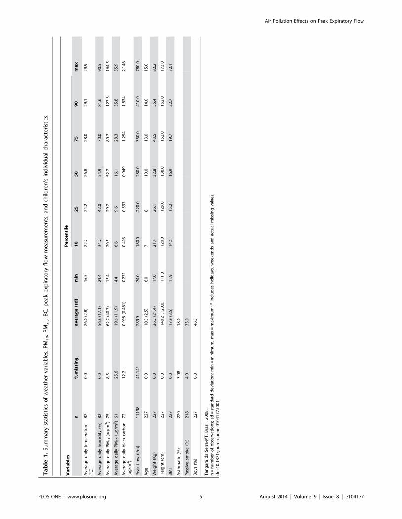
Tangara da Serra-MT, Brazil, 2008.*Model adjusted for age, BMI, gender, and asthma status; random coefficients for the intercept, time trend, humidity, and temperature; variance function of the randomerror included age, BMI, and asthma status.** Change in PEF for an increase of 10 mg/m3 in PM10lag1.HParametric Splines.doi:10.1371/journal.pone.0104177.t004
Air Pollution Effects on Peak Expiratory Flow
PLOS ONE | www.plosone.org 8 August 2014 | Volume 9 | Issue 8 | e104177
Ta
ble
5.
Esti
mat
ed
chan
ge
sin
pe
ake
xpir
ato
ryfl
ow
(in
l/m
in)
for
anin
cre
ase
of
10
mg/m
3in
PM
10
and
PM
2.5
and
anin
cre
ase
of
1mg
/m3
inb
lack
carb
on
for
all
child
ren
and
stra
tifi
ed
by
age
gro
up
s.
Ex
po
sure
All
Ch
ild
ren
(n=
22
0)
6to
8y
ea
rs(n
=6
9)
9to
11
ye
ars
(n=
69
)1
2to
15
ye
ars
(n=
82
)
Ch
an
ge
inP
EF
(95
%C
I)C
ha
ng
ein
PE
F(9
5%
CI)
Ch
an
ge
inP
EF
(95
%C
I)C
ha
ng
ein
PE
F(9
5%
CI)
PM
10
Lag
12
0.1
08
(20
.25
1;
0.0
35
)2
0.2
15
(20
.43
6;
0.0
06
)2
0.1
02
(20
.37
5;
0.1
72
)0
.08
2(2
0.1
75
;0
.33
8)
Lag
22
0.1
04
(20
.25
1;
0.0
42
)2
0.2
80
(20
.50
4;
20
.05
5)
20
.01
5(2
0.3
01
;0
.27
1)
0.1
00
(20
.16
2;
0.3
62
)
Lag
32
0.2
52
(20
.39
9;
20
.10
4)
20
.42
7(2
0.6
54
;2
0.1
99
)2
0.0
86
(20
.37
6;
0.2
05
)2
0.1
12
(20
.37
2;
0.1
48
)
Lag
42
0.1
96
(20
.32
2;
20
.07
0)
20
.28
3(2
0.4
77
;2
0.0
89
)2
0.1
39
(20
.38
5;
0.1
08
)2
0.1
25
(20
.34
7;
0.0
97
)
Lag
52
0.1
51
(20
.29
3;
20
.01
0)
20
.29
6(2
0.5
15
;2
0.0
77
)2
0.1
15
(20
.39
3;
0.1
62
)2
0.0
55
(20
.30
4;
0.1
95
)
Lag
0–
12
0.0
71
(20
.24
5;
0.1
03
)2
0.1
71
(20
.44
1;
0.0
99
)2
0.0
67
(20
.40
;0
.26
6)
0.1
17
(20
.19
1;
0.4
26
)
Lag
1–
22
0.1
26
(20
.28
4;
0.0
32
)2
0.2
98
(20
.54
0;
20
.05
5)
20
.06
3(2
0.3
70
;0
.24
5)
0.1
07
(20
.17
4;
0.3
88
)
Lag
0–
22
0.1
04
(20
.28
7;
0.0
78
)2
0.2
62
(20
.54
5;
0.0
21
)2
0.0
49
(20
.40
6;
0.3
09
)0
.12
3(2
0.2
01
;0
.44
7)
PM
2.5
Lag
10
.12
9(2
0.3
16
;0
.57
3)
0.1
08
(20
.57
6;
0.7
91
)0
.08
4(2
0.7
48
;0
.91
5)
0.1
75
(20
.59
0;
0.9
41
)
Lag
22
0.2
86
(20
.77
3;
0.2
01
)2
0.9
05
(21
.64
6;
20
.16
3)
0.2
02
(20
.70
0;
1.1
03
)0
.13
2(2
0.7
02
;0
.96
6)
Lag
32
0.3
77
(20
.79
2;
0.0
37
)2
0.3
22
(20
.95
4;
0.3
11
)2
0.5
58
(21
.33
1;
0.2
16
)2
0.1
91
(20
.92
6;
0.5
44
)
Lag
42
0.5
41
(20
.94
6;
20
.13
7)
20
.93
1(2
1.5
45
;2
0.3
17
)2
0.5
60
(21
.29
6;
0.1
75
)2
0.1
59
(20
.86
6;
0.5
49
)
Lag
52
0.0
29
(20
.48
7;
0.4
29
)2
0.1
37
(20
.83
5;
0.5
60
)0
.29
7(2
0.5
56
;1
.15
0)
20
.40
3(2
1.2
12
;0
.40
6)
PM
2.5
Imp
uta
tio
n
Lag
10
.13
4(2
0.2
83
;0
.55
0)
0.0
42
(20
.60
3;
0.6
88
)0
.26
9(2
0.5
31
;1
.07
0)
0.1
76
(20
.56
6;
0.9
18
)
Lag
22
0.1
81
(20
.60
1;
0.2
39
)2
0.5
81
(21
.22
7;
0.0
65
)0
.44
3(2
0.3
66
;1
.25
2)
20
.01
6(2
0.7
70
;0
.73
8)
Lag
32
0.4
62
(20
.86
2;
20
.06
2)
20
.43
3(2
1.0
43
;0
.17
8)
20
.51
5(2
1.2
94
;0
.26
3)
20
.25
3(2
0.9
65
;0
.45
9)
Lag
42
0.5
04
(20
.88
9;
20
.11
8)
20
.87
4(2
1.4
66
;2
0.2
83
)2
0.5
75
(21
.32
6;
0.1
75
)2
0.0
87
(20
.77
5;
0.6
00
)
Lag
52
0.0
51
(20
.47
8;
0.3
77
)2
0.4
74
(21
.13
5;
0.1
86
)0
.20
1(2
0.6
20
;1
.02
2)
20
.01
7(2
0.7
76
;0
.74
3)
Lag
0–
10
.26
1(2
0.2
31
;0
.75
3)
0.2
98
(20
.46
3;
1.0
58
)0
.30
1(2
0.6
44
;1
.24
6)
0.2
42
(20
.63
6;
1.1
22
)
Lag
1–
22
0.0
94
(20
.61
6;
0.4
29
)2
0.4
80
(21
.12
7;
0.7
49
)0
.50
9(2
0.4
96
;1
.51
4)
0.0
50
(20
.87
6;
0.9
75
)
Lag
0–
20
.04
8(2
0.5
56
;0
.65
1)
20
.18
9(2
1.1
27
;0
.74
9)
0.5
35
(20
.62
3;
1.6
93
)0
.11
5(2
0.9
52
;1
.18
1)
BC
Lag
10
.61
0(2
0.4
35
;1
.65
5)
1.9
50
(0.3
23
;3
.57
7)
0.1
20
(21
.76
2;
2.0
02
)2
0.7
30
(22
.59
2;
1.1
32
)
Lag
20
.07
4(2
1.2
84
;1
.43
2)
0.6
30
(21
.46
7;
2.7
27
)0
.47
0(2
1.9
80
;2
.92
0)
21
.33
0(2
3.7
60
;1
.10
0)
Lag
32
0.2
77
(21
.63
5;
1.0
81
)2
0.9
00
(22
.97
8;
1.1
78
)0
.64
0(2
1.8
10
;3
.09
0)
20
.43
0(2
2.8
80
;2
.02
0)
Lag
42
1.3
96
(22
.49
9;
20
.29
3)
22
.14
0(2
3.8
26
;2
0.4
54
)2
1.2
00
(23
.18
0;
0.7
80
)2
0.0
60
(22
.05
9;
1.9
39
)
Lag
52
1.5
39
(22
.52
5;
20
.55
3)
22
.51
0(2
4.0
19
;2
1.0
01
)2
1.8
80
(23
.64
4;
20
.11
6)
0.2
00
(21
.58
4;
1.9
84
)
Lag
0–
11
.42
8(0
.23
0;
2.6
26
)2
.63
0(0
.76
8;
4.4
92
)0
.94
0(2
1.2
16
;3
.09
6)
0.0
80
(22
.03
7;
2.1
97
)
Lag
1–
20
.62
0(2
0.7
05
;1
.94
5)
1.9
20
(20
.15
8;
3.9
98
)0
.37
0(2
2.0
02
;2
.74
2)
21
.07
0(2
3.4
42
;1
.30
2)
Lag
0–
21
.41
0(2
0.0
05
;2
.82
5)
2.8
54
(0.6
39
;5
.06
9)
0.9
50
(21
.57
8;
3.4
78
)2
0.3
10
(22
.81
9;
2.1
99
)
Tan
gar
ad
aSe
rra-
MT
,B
razi
l–
20
08
.d
oi:1
0.1
37
1/j
ou
rnal
.po
ne
.01
04
17
7.t
00
5
Air Pollution Effects on Peak Expiratory Flow
PLOS ONE | www.plosone.org 9 August 2014 | Volume 9 | Issue 8 | e104177
Ta
ble
6.
Esti
mat
ed
chan
ge
sin
pe
ake
xpir
ato
ryfl
ow
(in
l/m
in)
for
anin
cre
ase
of
10
mg/m
3in
PM
10
and
PM
2.5
and
anin
cre
ase
of
1mg
/m3
inb
lack
carb
on
for
all
child
ren
and
stra
tifi
ed
by
age
gro
up
s,ac
cord
ing
toP
DLM
bas
ed
on
the
exp
osu
res
of
the
curr
en
td
ayto
the
pre
vio
us
3d
ays.
Ex
po
sure
All
Ch
ild
ren
(n=
22
0)
6to
8y
ea
rs(n
=6
9)
9to
11
ye
ars
(n=
69
)1
2to
15
ye
ars
(n=
82
)
Ch
an
ge
inP
EF
(95
%C
I)C
ha
ng
ein
PE
F(9
5%
CI)
Ch
an
ge
inP
EF
(95
%C
I)C
ha
ng
ein
PE
F(9
5%
CI)
PM
10
Lag
00
.03
7(2
0.1
61
;0
.23
6)
0.1
25
(20
.17
4;
0.4
25
)0
.04
7(2
0.3
21
;0
.41
4)
20
.10
7(2
0.4
65
;0
.25
2)
Lag
10
.06
6(2
0.0
54
;0
.18
6)
0.0
23
(20
.16
1;
0.2
07
)2
0.0
34
(20
.25
8;
0.1
90
)0
.20
6(2
0.0
06
;0
.41
9)
Lag
22
0.0
30
(20
.15
0;
0.0
89
)2
0.1
35
(20
.31
6;
0.0
46
)2
0.0
66
(20
.28
8;
0.1
56
)0
.14
8(2
0.0
68
;0
.36
4)
Lag
32
0.2
52
(20
.42
9;
20
.07
5)
20
.34
9(2
0.6
23
;2
0.0
76
)2
0.0
50
(20
.38
1;
0.2
81
)2
0.2
81
(20
.59
1;
0.0
28
)
Ove
rall
20
.17
9(2
0.3
90
;0
.03
1)
20
.33
6(2
0.6
61
;2
0.0
10
)2
0.1
04
(20
.49
6;
0.2
88
)2
0.0
34
(20
.40
2;
0.3
35
)
PM
2.5
Lag
00
.19
9(2
0.2
70
;0
.66
9)
0.5
61
(20
.14
7;
1.2
69
)2
0.0
72
(20
.92
6;
0.7
81
)0
.01
8(2
0.8
34
;0
.87
0)
Lag
10
.08
4(2
0.2
10
;0
.37
8)
20
.16
3(2
0.6
13
;0
.28
8)
0.3
68
(20
.17
0;
0.9
06
)0
.12
1(2
0.4
02
;0
.64
5)
Lag
22
0.1
19
(20
.43
2;
0.1
95
)2
0.4
43
(20
.92
1;
0.0
34
)0
.21
6(2
0.3
57
;0
.78
9)
0.0
12
(20
.54
9;
0.5
74
)
Lag
32
0.4
08
(20
.80
9;
20
.00
7)
20
.28
1(2
0.8
93
;0
.33
1)
20
.52
8(2
1.2
66
;0
.20
9)
20
.30
8(2
1.0
22
;0
.40
6)
Ove
rall
20
.24
3(2
0.9
22
;0
.43
5)
20
.32
6(2
1.3
73
;0
.72
0)
20
.01
6(2
1.2
67
;1
.23
4)
20
.15
6(2
1.3
52
;1
.04
0)
BC
Lag
01
.79
7(0
.50
4;
3.0
90
)1
.76
0(2
0.2
26
;3
.74
6)
1.7
74
(20
.51
1;
4.0
59
)1
.75
3(2
0.5
74
;4
.08
2)
Lag
10
.11
1(2
0.7
19
;0
.94
2)
0.9
63
(20
.30
9;
2.2
35
)2
0.2
86
(21
.75
1;
1.1
79
)2
0.7
71
(22
.27
8;
0.7
37
)
Lag
22
0.5
66
(21
.48
4;
0.3
52
)0
.06
9(2
1.3
55
;1
.49
4)
20
.73
3(2
2.3
53
;0
.88
8)
21
.30
4(2
2.9
45
;0
.33
6)
Lag
32
0.2
35
(21
.64
9;
1.1
79
)2
0.9
20
(23
.07
2;
1.2
32
)0
.43
4(2
2.0
66
;2
.93
5)
0.1
52
(22
.43
3;
2.7
37
)
Ove
rall
1.1
08
(20
.73
9;
2.9
55
)1
.87
3(2
1.0
31
;4
.77
7)
1.1
89
(22
.09
1;
4.4
70
)2
0.1
69
(23
.42
7;
3.0
89
)
Tan
gar
ad
aSe
rra-
MT
,B
razi
l–
20
08
.d
oi:1
0.1
37
1/j
ou
rnal
.po
ne
.01
04
17
7.t
00
6
Air Pollution Effects on Peak Expiratory Flow
PLOS ONE | www.plosone.org 10 August 2014 | Volume 9 | Issue 8 | e104177
Ta
ble
7.
Esti
mat
ed
chan
ge
sin
pe
ake
xpir
ato
ryfl
ow
(in
l/m
in)
for
anin
cre
ase
of
10
mg/m
3in
PM
10
and
PM
2.5
and
anin
cre
ase
of
1mg
/m3
inb
lack
carb
on
for
all
child
ren
and
stra
tifi
ed
by
age
gro
up
s,ac
cord
ing
toP
DLM
bas
ed
on
the
exp
osu
res
of
the
curr
en
td
ayto
the
pre
vio
us
5d
ays.
Ex
po
sure
All
Ch
ild
ren
(n=
22
0)
6to
8y
ea
rs(n
=6
9)
9to
11
ye
ars
(n=
69
)1
2to
15
ye
ars
(n=
82
)
Ch
an
ge
inP
EF
(95
%C
I)C
ha
ng
ein
PE
F(9
5%
CI)
Ch
an
ge
inP
EF
(95
%C
I)C
ha
ng
ein
PE
F(9
5%
CI)
PM
10
Lag
00
.04
6(2
0.1
11
;0
.20
2)
0.0
76
(20
.16
2;
0.3
13
)2
0.0
39
(20
.33
0;
0.2
52
)0
.04
0(2
0.2
41
;0
.32
1)
Lag
10
.01
2(2
0.0
46
;0
.07
0)
20
.04
5(2
0.1
34
;0
.04
5)
20
.02
2(2
0.1
30
;0
.08
7)
0.0
38
(20
.06
4;
0.1
40
)
Lag
22
0.0
56
(20
.12
5;
0.0
13
)2
0.1
24
(20
.22
9;
20
.01
9)
20
.02
0(2
0.1
49
;0
.10
8)
0.0
22
(20
.10
2;
0.1
45
)
Lag
32
0.0
85
(20
.15
8;
20
.01
2)
20
.16
1(2
0.2
72
;2
0.0
51
)2
0.0
35
(20
.17
1;
0.1
00
)2
0.0
08
(20
.13
9;
0.1
22
)
Lag
42
0.0
99
(20
.15
3;
20
.04
6)
20
.15
7(2
0.2
40
;2
0.0
74
)2
0.0
66
(20
.16
6;
0.0
33
)2
0.0
52
(20
.14
5;
0.0
41
)
Lag
52
0.1
00
(20
.22
8;
0.0
29
)2
0.1
12
(20
.30
8;
0.0
84
)2
0.1
13
(20
.35
2;
0.1
25
)2
0.1
09
(20
.33
9;
0.1
20
)
Ove
rall
20
.30
6(2
0.5
64
;2
0.0
48
)2
0.5
23
(20
.92
2;
20
.12
4)
20
.29
6(2
0.7
75
;0
.18
4)
20
.07
0(2
0.5
22
;0
.38
2)
PM
2.5
Lag
00
.32
1(2
0.0
70
;0
.71
1)
0.2
88
(20
.30
6;
0.8
82
)0
.43
5(2
0.2
77
;1
.14
6)
0.1
64
(20
.53
8;
0.8
67
)
Lag
12
0.0
14
(20
.19
7;
0.1
69
)2
0.0
53
(20
.33
5;
0.2
29
)0
.05
7(2
0.2
81
;0
.39
5)
0.0
08
(20
.31
4;
0.3
31
)
Lag
22
0.2
11
(20
.41
8;
20
.00
3)
20
.28
0(2
0.5
99
;0
.03
9)
20
.15
6(2
0.5
41
;0
.22
9)
20
.08
3(2
0.4
49
;0
.28
3)
Lag
32
0.2
70
(20
.47
6;
20
.06
4)
20
.39
3(2
0.7
08
;2
0.0
78
)2
0.2
03
(20
.58
4;
0.1
78
)2
0.1
09
(20
.47
3;
0.2
55
)
Lag
42
0.1
91
(20
.36
3;
20
.02
0)
20
.39
2(2
0.6
59
;2
0.1
26
)2
0.0
85
(20
.40
1;
0.2
32
)2
0.0
70
(20
.37
0;
0.2
31
)
Lag
50
.02
4(2
0.3
50
;0
.39
9)
20
.27
8(2
0.8
55
;0
.29
9)
0.1
93
(20
.49
1;
0.8
76
)0
.03
4(2
0.6
29
;0
.69
7)
Ove
rall
20
.34
0(2
1.2
06
;0
.52
6)
21
.10
9(2
2.4
48
;0
.23
1)
0.2
47
(21
.33
9;
1.8
33
)2
0.0
55
(21
.58
6;
1.4
76
)
BC
Lag
00
.83
1(2
0.1
74
;1
.83
6)
0.9
68
(20
.59
2;
2.5
29
)0
.44
1(2
1.3
45
;2
.22
7)
0.9
10
(20
.88
5;
2.7
05
)
Lag
10
.33
9(2
0.1
03
;0
.78
2)
0.6
68
(20
.03
3;
1.3
70
)0
.23
8(2
0.5
51
;1
.02
7)
20
.08
7(2
0.8
62
;0
.68
8)
Lag
22
0.0
85
(20
.71
0;
0.5
40
)0
.24
5(2
0.7
29
;1
.21
9)
20
.73
3(2
1.8
42
;0
.37
7)
20
.63
3(2
1.7
47
;0
.48
2)
Lag
32
0.4
42
(21
.09
2;
0.2
08
)2
0.3
02
(21
.31
1;
0.7
08
)2
0.2
88
(21
.44
2;
0.8
65
)2
0.7
28
(21
.89
2;
0.4
36
)
Lag
42
0.7
31
(21
.21
8;
20
.24
5)
20
.97
2(2
1.7
39
;2
0.2
04
)2
0.6
11
(21
.47
7;
0.2
56
)2
0.3
73
(21
.23
4;
0.4
89
)
Lag
52
0.9
53
(21
.90
2;
20
.00
4)
21
.76
5(2
3.2
60
;2
0.2
71
)2
0.9
73
(22
.65
7;
0.7
10
)0
.43
4(2
1.2
39
;2
.10
6)
Ove
rall
21
.04
0(2
3.3
01
;1
.22
0)
21
.15
7(2
4.7
95
;2
.48
2)
21
.19
8(2
5.2
44
;2
.84
8)
20
.47
6(2
4.3
80
;3
.42
8)
Tan
gar
ad
aSe
rra-
MT
,B
razi
l–
20
08
.d
oi:1
0.1
37
1/j
ou
rnal
.po
ne
.01
04
17
7.t
00
7
Air Pollution Effects on Peak Expiratory Flow
PLOS ONE | www.plosone.org 11 August 2014 | Volume 9 | Issue 8 | e104177
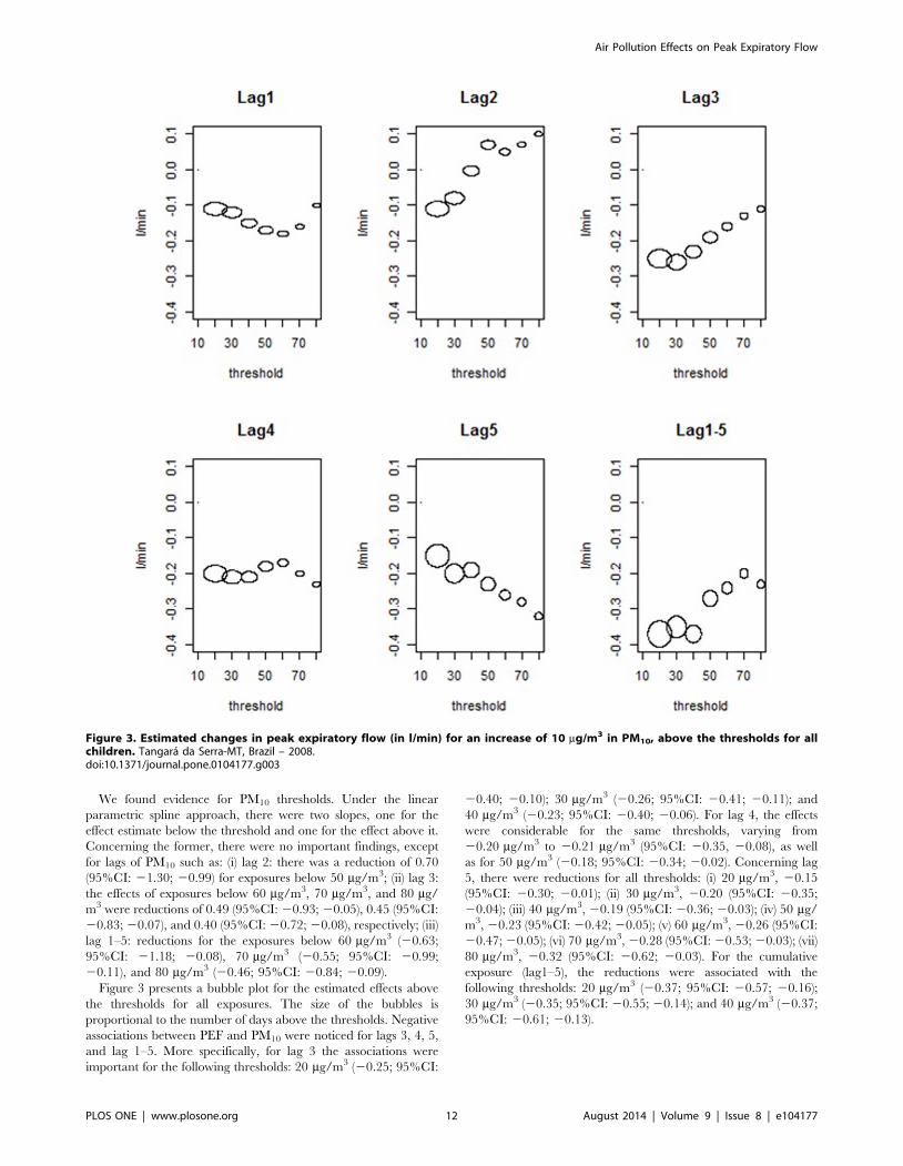
We found evidence for PM10 thresholds. Under the linear
parametric spline approach, there were two slopes, one for the
effect estimate below the threshold and one for the effect above it.
Concerning the former, there were no important findings, except
for lags of PM10 such as: (i) lag 2: there was a reduction of 0.70
(95%CI: 21.30; 20.99) for exposures below 50 mg/m3; (ii) lag 3:
the effects of exposures below 60 mg/m3, 70 mg/m3, and 80 mg/
m3 were reductions of 0.49 (95%CI: 20.93; 20.05), 0.45 (95%CI:
20.83; 20.07), and 0.40 (95%CI: 20.72; 20.08), respectively; (iii)
lag 1–5: reductions for the exposures below 60 mg/m3 (20.63;
80 mg/m3, 20.32 (95%CI: 20.62; 20.03). For the cumulative
exposure (lag1–5), the reductions were associated with the
following thresholds: 20 mg/m3 (20.37; 95%CI: 20.57; 20.16);
30 mg/m3 (20.35; 95%CI: 20.55; 20.14); and 40 mg/m3 (20.37;
95%CI: 20.61; 20.13).
Figure 3. Estimated changes in peak expiratory flow (in l/min) for an increase of 10 mg/m3 in PM10, above the thresholds for allchildren. Tangara da Serra-MT, Brazil – 2008.doi:10.1371/journal.pone.0104177.g003
Air Pollution Effects on Peak Expiratory Flow
PLOS ONE | www.plosone.org 12 August 2014 | Volume 9 | Issue 8 | e104177
Discussion
This study’s results suggest that air pollution from biomass
burning may be a respiratory health risk factor for schoolchildren
aged 6 to 15 years old living in the Brazilian Amazon. This
association is consistent with the previous panel study undertaken
in the municipality of Alta Floresta [10]. The current study
extended previous analyses by including PDLM as well as adding
the effects of BC and PM10 exposures. Further, we explored two
methods for analysing panel studies: MEM and univariate time
series modelling, which was applied to every child. Although the
combined-effect estimates obtained using the univariate approach
and those from MEM were similar, their precision was different.
However, it was particularly important to show that some students
were more vulnerable to air pollution than were others.
Our findings corroborate the results of panel studies describing
a linear effect of air pollution on PEF [5], [8], [29]. No association
was found with PM2.5 or BC in a rural panel study undertaken in
the southeast of Brazil to investigate the effects of pre-harvest
sugarcane burning on PEF [30]. Systematic reviews of panel
studies demonstrated negative pooled effects of PM10 and PM2.5
on PEF [31], [32], [33].
Although we found associations for all children, the effects were
stronger after stratification by age, with PEF decrements for the
youngest group, confirming that younger children are more
susceptible to air pollution effects [1]. In the Alta Floresta study
[10], a negative association of PM2.5 with PEF was found for
children who studied in the afternoon. However, the authors noted
that the majority of children in this group were from 6 to 9 years
old. Our results confirm the hypothesis that age is most likely to
explain this finding.
A multitude of factors are related to children’s PEF. In the
present study, PEF measurements were associated with temper-
ature, humidity, BMI, age, sex, and asthma status. Weather
conditions can influence children’s health [34] but also interfere
with pollutants in the atmosphere [35]. Other environmental
factors could affect PEF, for instance, time spent outdoors and
passive smoking. However, in this study these variables were not
important in the modelling, most likely because in the dry season
children spend most of their time outdoors when they are not at
school because of lack of leisure indoors as well as the high
temperatures.
Most adverse effects found in this study were lagged by 3, 4, and
5 days. Lagged effects as well as cumulative effects are expected in
this region not only because of the characteristics of Amazon
biomass burning (every day during the dry season) but also
because of meteorological factors, which allow for pollutants to
remain in the atmosphere for long periods of time. The PDLM
approach allowed exploring the effect of air pollutants on PEF
distributed over time and also the overall effect up to 3 or 5 lagged
days. The results revealed negative associations between air
pollution and PEF, mainly for PDLM 0–5, which is consistent with
the Mexico City panel study that found reductions in children’s
PEF associated with O3, PM2.5, and PM10 [21]. In the literature,
this methodology had been broadly applied in time series studies
[26] but not as much in children’s panel studies.
The PM10 effect was scrutinised using different thresholds. Our
results suggest hazardous effects below 50 mg/m3. For lag 5, there
was a clear negative gradient. The World Health Organisation
guidelines for PM10 are 20 mg/m3 for the annual average and
50 mg/m3 for the daily average in urban areas [2]. During the
2008 dry season in Tangara da Serra, approximately 53% of the
measurements were above 50 mg/m3.
This study could be taken into consideration by the Brazilian
Ministry of Health and other health agencies to establish
guidelines for health protection in regions where biomass burning
takes place. Reducing air pollutant levels is a challenge for local
authorities; however, more effective actions should be taken to
minimise fires, such as intensified patrolling in the region, heavy
fines, policy reforms on taxes and credits, and tougher legislation
concerning land occupation conflicts.
Air pollution was measured at the local university campus that is
near the study school. In fact, all study children lived within a
5 km distance from the university campus. We believe that the
device location did not sub or super estimated the observed
adverse effects because particles emitted through biomass burning
have relatively long resident time in the atmosphere and can be
transported over long distances, crossing international boundaries
[18]. This study would have benefited from a more specific
questionnaire, for instance to evaluate patterns of physical activity
and time spent outdoors.
In conclusion, this study showed a negative association between
exposure to air pollution and PEF in schoolchildren living in
Tangara da Serra. The analysis per child indicated that age was an
effect modifier and that air pollution mostly affects younger
children.
Acknowledgments
This paper is a contribution of the Brazilian National Institute of Science
and Technology (INCT) for Climate Change. The authors would like to
thank Beatriz Fatima Alves de Oliveira for the logistical support and Jose
Eduardo Ernesto Pinheiro from Universidade Federal do Rio de Janeiro
for the spirometry exams.
Author Contributions
Conceived and designed the experiments: LSVJ SSH EI ACMPL.
Performed the experiments: EI HAC PA PHNS. Analyzed the data: LSVJ
ACMPL. Contributed to the writing of the manuscript: LSVJ SSH HAC
EI PA PHNS ACMPL.
References
1. Pope CA, Dockery DW (2006) Health Effects of Fine Particulate Air Pollution:
Lines that Connect. J Air & Waste Manage Assoc 56: 709–742.
2. WHO (World Health Organization) (2005) Air quality guidelines for particulate
matter, ozone, nitrogen dioxide and sulfur dioxide. Global update 2005.
Summary of risk assessment. Geneva.
3. Cohen AJ, Anderson HR, Ostro B, Pandey KD, Krzyzanowski M, et al. (2004)
Urban Air Pollution. In: Ezzati M, Lopez AD, Rodgers A, Murray CJL.
Comparative Quantificatio Of Health Risks. Global and Regional Burden of
Disease Attributable to Selected Major Risk Factors. Vol. 2, Chapter: 17.
4. Jedrychowski WA, Perera FP, Maugeri U, Mroz E, Klimaszewska-Rembiasz M,
et al. (2010) Effect of prenatal exposure to fine particulate matter on ventilatory
lung function of preschool children of non-smoking mothers. Paediatr Perinat
Epidemiol 24(5):492–501.
5. Castro HA, Cunha MF, Mendonca GAS, Junger WL, Cunha-Cruz J, et al.
(2009) Effect of air pollution on lung function in schoolchildren in Rio de
Janeiro, Brazil. Rev Saude Publ 43: 26–34.
6. Gotschi T, Heinrich J, Sunyer J, Kunzli N (2008) Long-Term Effects of Ambient
Air Pollution on Lung Function: A Review. Epidemiol 19: 690–701.
7. Escamilla-Nunez MC, Barraza-Villarreal A, Hernandez-Cadena L, Moreno-
Macias H, Ramirez-Aguilar M, et al. (2008) Traffic-related air pollution and
respiratory symptoms among asthmatic children, resident in Mexico City: the
EVA cohort study. Respir Res 9: 74.
8. Epton MJ, Dawson RD, Brooks WM, Kingham S, Aberkane T, et al. (2008) The
effect of ambient air pollution on respiratory health of school children: a panel
study. Environ Health 7: 16.
9. PAHO (Pan American Health Organization) (2005) An Assessment of Health
Effects of Ambient Air Pollution in Latin America and the Caribbean.
Washington, DC.
Air Pollution Effects on Peak Expiratory Flow
PLOS ONE | www.plosone.org 13 August 2014 | Volume 9 | Issue 8 | e104177
10. Jacobson LSV, Hacon SS, Castro HA, Ignotti E, Artaxo P, et al. (2012)
Association between fine particulate matter and the peak expiratory flow ofschoolchildren in the Brazilian subequatorial Amazon: a panel study. Environ
Res 117: 27–35.
11. Sisenando HA, Batistuzzo de Medeiros SR, Artaxo P, Saldiva PH, Hacon SS(2012) Micronucleus frequency in children exposed to biomass burning in the
Brazilian Legal Amazon region: a control case study. BMC Oral Health 12: 6.12. Ignotti E, Hacon SS, Junger WL, Mourao D, Longo K, et al. (2010) Air
pollution and hospital admissions for respiratory diseases in the subequatorial
Amazon: a time series approach. Cad Saude Publica 26(4):747–61.13. Carmo CN, Hacon S, Longo KM, Freitas S, Ignotti E, et al. (2010) Association
between particulate matter from biomass burning and respiratory diseases in thesouthern region of the Brazilian Amazon. Rev Panam Salud Publica 27(1):10–6.
14. Silva AMC, Mattos IE, Freitas SR, Longo KM, Hacon SS (2010) Materialparticulado (PM2.5) de queima de biomassa e doencas respiratorias no sul da
Amazonia brasileira. Rev Bras Epidemiol 13(2):337–51.
15. Mascarenhas MDM, Vieira LC, Lanzieri TM, Leal APPR, Duarte AF, et al.(2008) Poluicao atmosferica devido a queima de biomassa florestal e
atendimentos de emergencia por doenca respiratoria em Rio Branco, Brasil –setembro, 2005. J Bras Pneumol 34: 42–46.
16. Fundacao Instituto Brasileiro de Geografia e Estatıstica – IBGE (2010) Censo