AD-Ai69 958 NONPARAIIETRIC SEQUENTIAL ESTIMATION OF ZEROS AND i/I EXTRENA OF REGRESSION FU (U) NORTH CAROLINA UNIV AT CHAPEL HILL CENTER FOR STOCHASTIC PROC N HAERDLE UNCLASSIFIED JAN 86 TR-i33 AFOSR-TR-86-84e8 F/G 12/1 NL Eu..".l
Transcript
AD-Ai69 958 NONPARAIIETRIC SEQUENTIAL ESTIMATION OF ZEROS AND i/I
EXTRENA OF REGRESSION FU (U) NORTH CAROLINA UNIV ATCHAPEL HILL CENTER FOR STOCHASTIC PROC N HAERDLE
UNCLASSIFIED JAN 86 TR-i33 AFOSR-TR-86-84e8 F/G 12/1 NL
Eu..".l
.12.
..
1L2 132 1.
,amm
i-
3 -F D
I.
~MICROCOPY RESOLUTION TEST CHART
NATIONAL BLUR[AU OF SIANBARDS IPR3 A
.'o *I°-°
. *o.%.":...1..
-p-°sp.:;,,a. .
p,% '
.FOSR-T T - 8 - a 0 4 0 0..
CENTER FOR STOCHASTIC PROCESSES
00.I%
In .Department of Statistics
University of North CarolinaChapel Hill, North Carolina
NONPARAMETRIC SEQUENTIAL ESTIMATION OF ZEROS AND EXTREMA
Let (X, Y), (Xi, Y1), (X 2, Y2 ).... be a sequence of independent, identically distributed, bi-variate randoiii variables with joint probaility deusity fuanct ion f(x, y). In tis paper we coiisiderthe seqluentid ,stilnation of zeros Aid extreiia of ir(z) = E(YIX = x) using a Conlinatiol of
the nonparametric kernel and stochaw.tic al)lroximalt ion methods. The structure of our sampling
scheme is dilfferent from the one considered by lRohbiis Land Monro (1951) since the experimenter,observing the bivariate data, has no control over the design variables {X,}, as is assumed in
classical stochastic approximation algorithms.
The proposed sequential procedure is based on the principal idea of nonparametric kernel
estimation of re(z), i.e. to construct a weighted average of those observat ions (X,, I) of which
X, happens to fall into an asymptotically shrinking neighborhood of x. The shrinkage of such a
neighborhood is usually parameterized by a seqtence of bandwidths h,, tending to zero, whereas
the shape of the neighborhoods is given by a real kcrnte functC ,n K.
Motivated by classical procedures we define the following sequential estimator of a zero of
M7,
(1) Z = 2, -anh 'K((Z. - X,,)/h,, , 1.
*Her, Zi denotes an arbitrary starting random variable with finite second moment and {an} isa Sequence of positive constants tending to zero. I fact, the sequence { Z. } will converge under
our conditions to the (unique) zero of
(X) f yf (x, y)dy = m(x)fx (z),
where fx(z) denotes the marginal density of X, but an assumption about fx ensures that the
zero of the two functions m and ri is identical.
Under mild conditions we show consistency (almost surely and in quadratic mean) and
asymptotic normality of {Z}. An asymptotic bias term (depending on the smoothness of n)
, shows ip, if the bandwidth sequence tends to zero at a specific rate. Fixed width confidence
intervals are constructed, using a suitable stopping rule based on estimates of the variance of
the asymptotic normal distribution.
Our arguments canl be extended to the problem of estimating extremal values of the regres-
.ion function m. Note that m = fi/fx and therefore rn' =' /fk, where
T()= fX(X) f T ahx~f~
i ld'r a suitable assumption the problen of finding an extremum of m is equivalent to finding
.1 .[il ue) zero of the function r. So it is reasonable to apply a procedure similar to (1). Addi-tioi;U difficulties turn up since fx has to be estimated separately. We propose to perform the
estimation by an additional i.i.d. sequence {X,} with the same distribution as X. Define ]
We shall prove that {Z,} is consistent and asymptotically normally distributed. Fixed
wid h confidence intervals are computed by the same technique as for { Z,, }.
If we knew fx the algorithm (2) would simplify, the additional {X.} are obsolete in this
ca.se, here we propose
(3) Z', +I = Z - a. h K'((Z', - X,)/h,)Y,, fx(Z, )
+a,,h,'K((Z," - .\)/h,)Yfk.JZ,), -> 1.
The additional difficulty of estimating simultaneously fx didn't occur in the case of esti-
inatin.g zeros, since the problein for m could be transferred to the equivalent problem for th,
which does not involve fX. I practice the adti ioal i.i.d. sequence { X, } could be constructed
by saIIIhnl ig il pairs and diiscarding the Y olst-rvations of one element. This results in some
loss of etliciency but makes the practical application possible with the data at hand. Another
proposal that we would like to iiake is related to the boot-strap. From the first N observations,
a denisity estimate ]x of fx could be constructed and then the algorithm (2) could be started
W ith {X,} distributed with density fx. A third possibility is to plug in fx into the algorithm
(3). We (lid not investigate the last mentioned procedures.
An alternative way of defining an estimator of the zero of the regression function m could be
to construct an estimate of t he whole function ata( then to empirically determine an observed zero
as an e#stirnate. This procetdure would be time co7)sunJiing in the case of sequential observation
of the date, since for every new observation the whole function has to be constructed wherea;s
our procedure just keeps one number in meniory and updates that number due to the formal
presription (1). Also in cases where an enormous amount of data has to be processed, an estimate
of a ,ero based on the estimate of the whole regression function seems to be inadvisable sinceall the data has to be stored in the memory at a time.
Related work was done by Revesz (1977) arid Rutkowski (1981, 1982) who applied stochasticpa,,r(.xiiiation imethods to the estimation of m at a fixed point. Our derivation of fixed width
-'-,diice intervals was inspired by the papers of Chow and Robbins (1965), McLeish (1976)S.. Stur,'" 1980). The author last neltioned used in the field of density estimation the kernel
.-t r:.iti ii technique that introduces a localizinig effect which makes classical miethods, such as
\,.ti,.r' (1966), app)licalvl.
l'n,. rest of the paper is organized as follow.. Section 2 comtainus tle results and gives
ti, ,,:isteiicy proof for {Z,}. In section 3 we present the re.sults of some simulations and an
apl i at on f of {Z, } to sone real data. In the last section we give the rest. of the proofs.
i~%•
LON'
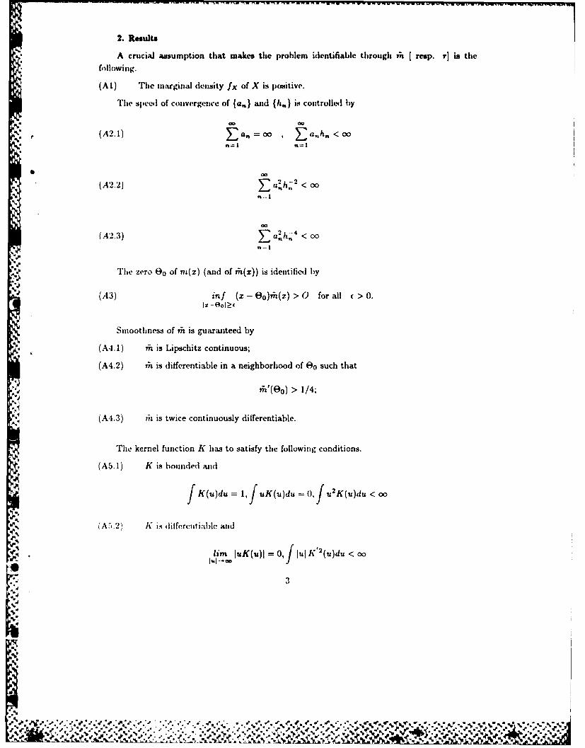
2. Results
A crucial assumption that makes the problem identifiable through in resp. r] is the
following.
(Al) The marginal density fx of X is pomitive.
The speed of convergence of (a.) and {h,.) is controlled by
(A2.1) au=oo , a,,hn < on=l n=l
a 00
(A2.2) 2h,2 < oo
00
(A2.3) ah - < 00
n . I
The zero 0 0 of rn(x) (and of in(x)) is identified by
(A3) inf (x - Oo)vh(x) > 0 for all > 0.
Smoothness of in is guaranteed by
(A4.1) fh is Lipschitz continuous;
(A4.2) rn is differentiable in a neighborhood of 00 such that
,n'(00) > 1/4;
(A4.3) ?h is twice continuously differentiable.
The kernel function K has to satisfy the following conditions.
(A5.1) K is bounded and
f K(u)du= 1,f uK(u)du =0, fu 2 K(u)du <0o
fA5.2t K is diileretiable and
lUr IuK(u)l = 0, lul K'2(u)du < o
3
.J°%
IILm
I~ #Z j.,#"l ) . I , . .r J
% %'
. ".' ,,, tl '.,," s ._ "-J 't -¢~ ' , t' " , .
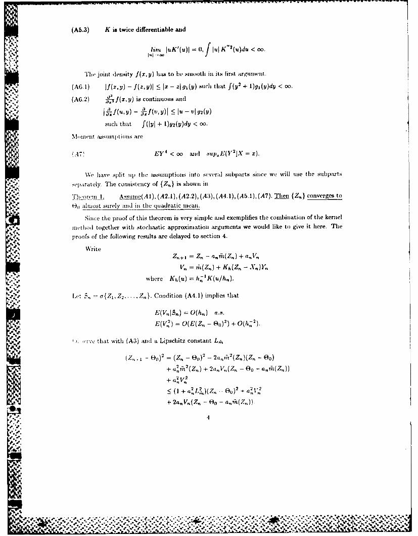
(A5.3) K is twice differentiable and
1ira luK'(u)l 0,1 ul K"2(u)du < oo.
The joint density f(x, y) has to be smooth in its first argilnent.
(A6. 1) if(x, y) - f(z, )l : Ix - z 91 (y) such that f(y 2 + 1)g1 (y)dy < oo.
(AG.2) -)f(x, y) is continuous and
f, f("fyY) -fl(,,Y) U U-V lY2(Y)
such that f(lyl + 1)g2(y)dy < oo.
M )ilent assmlp 'tions are
(.47) EY 4 < oo and supE(Y2jA = x).
We have split u l , tlhe Ssulniptions into several subparts since we will use the subparts
septrately. The consistency of {Z,) is shown in
lhoren 1. Assiiuie(Al),(A2.1),(A2.2),(A3),(A4.1),(A5.1),(A7). Then {Z,,} converges to
H,) almost surely and in the quadratic mean.
Since the proof of this theorem is very simple and exemplifies the combiniation of the kernel
nictliod together with stochastic approximation arguments we would like to give it here. The
proofs of the following results are delayed to section 4.
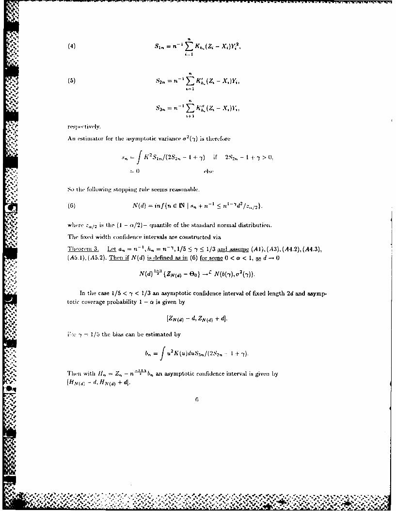
converges tinder our assumptions to T1eM, alnost surely. Define
- f K 2 f(K' )2S /(2.;2. - I + 4,1)
N (d) = (Y2 E LN + S,I± < " I 21-2-'Z,,',,.
Then para lel to 'The oremi 3 we have
'heorem 6. Let a,. = n I and h,, = < , -/ < y < 1/5, and let the condil ions of Theorem 5
h' fulfilhd. Then, as (I - 0
N'(d)l/22)Za Om } NZ/ (0, a.mf ')
'ii.
9%.
I -
3. Mont* Carlo Study and an Application
In this section we report the results of a Monte Carlo experiment comparing the performanceof our sequential procedure when some of the invOlV(l parameters are tuned at different levels.We also report aii application of the algorithm (1) to som1e reial data.
The bLsic experiment to assess the accuracy of lheorenm 3 consisted of 200 Monte CarloreplicationIs with the mnnbers N(d), ZN(,I) and S ,(,0 to be reported. Th'e joint probability den-
-,." sity function f(x, y) that we used was f(x,y ) = i) o((y - io(x))/o.), W the probabilitydhensity function of a standard normal distribution and r,(r) = -a{_( - X)2 - 1/4} for a = 4,8was the regresssion curve. We report the result for Z = 0.15 ('Fla;ble 1) and for Z1 = 0.2 (Table2). The paranieter or was set to o = 0.05. The zero th;t was to be eVSt.i1i;Lted was 00 o 1/2
0 and two different valuies of d and a. were fixed, naamely d = 0.05, 0.1 and a. 0.1, 1.0. As thekernel K we have chosen the Epanechnikov kernel K(u) = 3/4(1 - u2 ) for JI - I and K(u) = 0for Rl > 1. the sequnc'e of bandwidths was se't to h h,, = 7-, y = 0.21. In Table I theresults for the starting point Zi 0.45 are shown. The figures of Tablt I indicate that the fixed
* ;accuracy result
Table 1 abont .here
.ivn in Theorem 3 yields a good approximation of 0 0 even for ,d 0.1. This is seen from the
counts in the Zv(d)- column. It is indicated there how inany' times (from 200 Monte Carlotrials) the true parameter (0 = 1/2 was in the confidence interval [Zv(.t) - d, Z,(d) + d]. Asa measure of spread we added the quantiles Q95 and Q5 in the third and fourth column of
each entry. A small paradox occurs when we compare the fig-ures for different values of a. Itis expected that the procedure (1) stops earlier with a = 8 than with a = 4, since the higherderivative in the zero should speed up the convergence of {Z,,} to O0 . In both Table I and Table2 it is seen that the average of the stopping times
Table 2 about here
A"r 200 Monte Carlo runs) is considerably higher for a = 8 and o. = 0.1 than for a = 4 and(7. C) 1. This effect is due to the crude approximation var(YIX = X): a 2, X (o, as can be seen
fr. :n tine fignres for Sv(d). In the case of a = 8 the statistic SN(,d) considerably overestimatesthe true wsymptotic variance a(3'). For comparison we list some correct U(-y) = a(a., a, -). For
F osot:,,, 0(0.1,4,0.21) = 0.0(X)83 whereas o(0.1,8,0.21) = 0.00039.
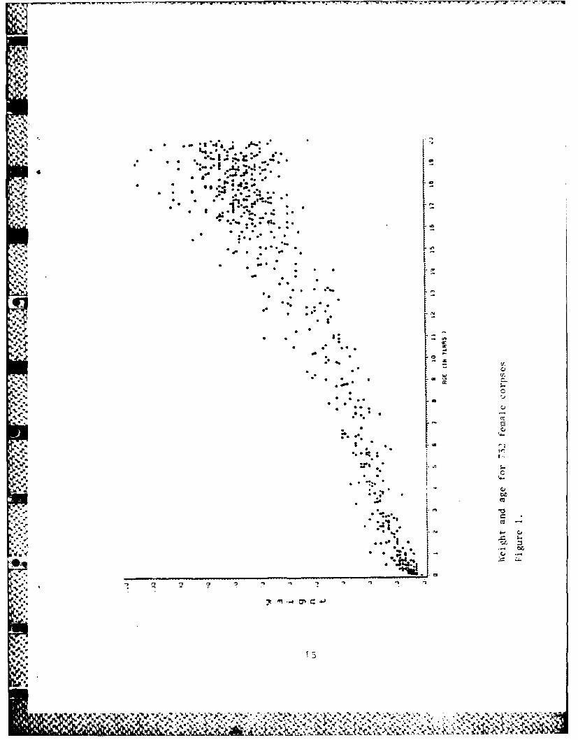
In a small application we took the sequence of random variables {(Xi, I') }, X. =age, Yj =weight
A,,%
V-
2€9
- .,.
of female corpses) which was gathered from 1969 to 1981 by the Institute of Forensic Medicineof Heidelberg. It is an interesting question in forensic medicine to estimate the mean age from
the weight of unknown corpses. We restricted our attention to the ages between 0 and 20 yearsin order to fulfill aLsu~mption (A3). We put m0 z 40 kg, and we applied the I)roceldirc (1) anid'ldled with differeit starting values ZI at ZN(d) = 11.6 years and N(d) = 563, for d = 0.1 andN(d) = 221 for d = 0.2(Z 1 = 0.4). A plot of tie first 732 dLta pairs, restricted to ages between( aod 20 years, should illustrate the accuracy of ZN(d) (Figure 1).
where W is the standard Wiener process starting at 0.
" Pr,,,f. I),'fjim"
5,, = a ,,,..., zn}
z.,,, - 00 = 0 - Dn/n)(z. - 0,) + n , + ,
where
_ = h-'/2 E{K( h )Y.IB.} - h-/ 2 K( h y,::: , .:,h h7, = n -2 {rn(Z.) - E[Kh(Z,. - X.)YIB.I}
and {B,0 } is a sequence of random variables converging almost surely to Vfh'(0 0 ) such that
B,(Z, - 00) = i(Z,,). Such a sequence exists because vh is differentiable in 0o and Z,- O0X Ialmost surely by Theorem 1. The assumption on a,, and h. imply that
--'. , 1/2fu2 K(u)dufi"(Oo). Note that E(V,0 B,,P) = 0 and that by (A7) and (A6.1),
E( IB,,) - f K2Jf, wdy, almost surely,
%. E(v,2) = O(1).
Furthermore we' have for all r > 0
ErV; (V ,I ) 5 O(h- P9 > ni,,)
< O(h-2 n - ') = o(1) almost surely.
% 'N'
4. OkL-4k
ir-- 11
I ,o,!. o".
The lemma follows now from the generalization of a theorem of Walk (1977) , given by
Berger (1980).
"ie following itina gives an iualogeous result for the Kiefer Wlfowitz typet sequence
(Z,,) dcfined ill (2)
Lemma 2. Let the conditions of Theorem, 6 be satisfied. Define IV,,(t) iLs ill Imma I but with
..- ill the place of ?h and
Rk = kl2 k'' : (Zk - OM).
Ihen W,,(t) converges weakly in C(O, 11 to the Gaussian process
;-(t)= fX(OM) J Y2 ff(0M, y)dy f K2 (K')2 f u(1, 11 )dW(tu), 0 < t < 1.
Proof of Theorem 2. Use Lemma I and evaluate G 1 (t) at t I.
Prooof of Theorem 3. Define the sequence
b(d) = inf {n E LN I <2_() 7,,( /Z
The estimators St,,, S 2,, defined in (4), (5) converge to f y2f(43, y)dy, 74'(0o) respectively. This
entails that, as d - 0,
N(d)/b(d) - 1 ahost surely.
Now apply Lemma 1.
Proof of Theorem 4. Like the proof of Theorem 1.
Proof of Theorem 5. Use Lemma 2 and evaluate G2 (t) at t = 1.
,, Proof of Theorem 6. Similar to the proof of Theorem 3..A
4
J.'
-.J.
-'. .
V. References
[1] Berger [19801: A note on the invariance principle for stochastic aIlprvxiuation in aHlilb'rt space. Manuscript.
[21 Chow, Y.S. and Rohbins, R. 119651: On the asymptotic theory of fixed- width sequential
confidence intervals for the memi. Ain. Math. Statist. 36, 457 462.
[3] McLeish, R. 11976]: Functional and random central limit theorems for the Robbins-Monro process. J. Appl. Prob. 13, 148-154.
[4] Nixdorf, R. 119821: Stochastische Approximation in Hilbertriumen durch endlichdimen-
sio ;de Verfahren. Mitt. Math. Sem. GieBen, Ileft 154.
[5] Revesz, P. [19771: How to apply the method of stochastic approximation in the non-parametric estimation of a regression function. Math. Oper. Statist. 8, 119-126.
J6 Robbins, 11. and Monro, S. [1951]: A stochastic approximation method. Ann. Math.
Statist. 22, 400-407.
[7] Rutkowski, L. [1981]: Sequenti,-d estimates of a regression function by orthogonal serieswith applications in discrimination. Lecture Notes in Statistics 8, Springer Verlag,
236 -244.
[8] Rutkowski, L. [19821: On-line identification of time- varying systems by nonparametrictechniques. IEEE trans. Autom Control. 27, 228-230.
[9] Stute, W. 119831: Sequential fixed-with confidence intervals for a non-parametric densityfunction. Z. Wahrsch. 62, 113-123.
[10 Venter, J.H. [1966]: On Dvoretzky stochastic approximation theorems. Ann. Math.Statist. 37, 1534-1544.
[11 Walk, H. [1977]: An invariance principle for the Robbins- Monro process in a Hilbert
space. Z. Wahrsch. 39, 135-150.
.J1
% %%
-.
-,,"%,-
-,RV- 7- M P4
6 33
i- LI' L' u' LI u LI' L LII U
o~I - '6.. 0 '.-L, -3 - .3 LI i ON 0 I 0 11a l cl, ON Z. toJ w~ m
t) as 1 , L _ l% .*rj w % i i
A- M~ A a - - n wA Db L ka An- -
co D. 0n *j 10w X.iP
01 -n 30 l 4 " - C
-.3 C. o. t) LICo' - r
A ('0 ni 0 co i ' a '.o ~ 0 Vi 0 -j tU Li' U' .DCN 0O 0 00 w ~ (-n L' . -j3 - a' D. 0 .0 ON .r
N.) 0 L, , ZNIj LI C" LI' w~ m -. Ln LI' j. '0 Lu '
) X. L U W W)3 f
N N
m T
ID L n ON-. -. I' aN a' .Z. C"n %D LP D- M -J a'UA N) W' A Q -j C, 6-' m N. J '.0 w. ~
-~ 1 Dm 1 4 w 30
0 m 0I LaN -b I -. w'M0 a n rK ) Aj CD4 L
m) -l. -n - (. -i - -)
LZa K) C O A~ a'n fl) '.0K -i m A a' a .
z fi -1 un LA w Ul N 0 C) W X. fl CLpun - "o j x A. M w . r- tn o C