ADAID1 676 CHUTE-STOFFA INC NYACK NY F/ 20/1 DESIGN CRITERIA FOR A DEEP TOWED SOURCE AND MULTI-CHANNEL ARRAY-ETC(Ul JUL 79 N0001479-H-0090 EErlhshEIhErhEE EEE 'I/// E I//I EE //E/IEEE/IE/IIE I/EII/I//I
Transcript
ADAID1 676 CHUTE-STOFFA INC NYACK NY F/ 20/1DESIGN CRITERIA FOR A DEEP TOWED SOURCE AND MULTI-CHANNEL ARRAY-ETC(Ul
JUL 79 N0001479-H-0090
EErlhshEIhErhEEEEE'I / / / EI / / I EE//E/IEEE/IE/IIEI/EII/I//I
~LEvE v
(c DESIG SRITRIA FOR A_9EP OWED SOURCE
and w- ,,ULTI-CfANNLL ARRAY.
) ,N
Chute Stoffa, Inc.AJ2 3 viifay 19 79
Revised: 16 July 1979
81 7 21 028
I I
]S U10ARY
- -The accuracy of sedimentary interval velocities
derived from a towed hydrophone array can be predicted in the
ideal case of horizontal interfaces and an idealized source
]pulse. The parameters of the prediction model are the two-way
]normal-incidence travel time and RMS velocity to the horizon ofinterest, array length, and source pulse width. First, the
]range of RMS velocities likely to be encountered in the upper
500 m of sediments is determined. Second, the error in these
]RMS velocity measurements is calculated as a function of array
-,length, height above the sea floor and pulse width. Third,
the R S velocity error is converted to interval velocity error
as a function of layer thickness and velocity, pulse width,
and array length and height. It should be emphasized that these
errors do not include any additional errors generated by the
hyperbolic travel-time assumption and do not include the degrada-
-J tion encountered for dipping layers. In addition, our discussion
] refers to the analysis of one Common Shot Point or Common
Depth Point Gather. Considerable improvement in an average
] -interval velocity determination can be obtained by the analysis
of several nearby CSP's or CDP's. This improvement will depend
on lateral continuity for the horizons of interest. In the
] discussion which follows, we emphasize that only one CDP or
CSP is being considered.
]A short pulse, long array, small height above the
sea floor all will contribute to increased interval velocity
II
L .....
-2-
resolution. A 1 km long array and a source with a 2 millisecond
pulse width, both towed 100 meters above the sea floor, can yield
interval velocities with errors of 2 percent for beds extending
from 50 to 500 m below the sea floor. For beds thinner than
50 meters the error increases rapidly, becoming approximately
A 10 percent for 20 m beds. For beds greater than 200 m thick
whose tops are 400 meters below the sea floor the error is 8
percent. Again the error increases rapidly for thinner beds.
For an array altitude of 500 m the minimun error is 7 percent
and this increases rapidly for beds thinner than 150 m.
SA I km long array, 2 millisecond source pulse, and
a tow altitude of 100 m is recommended to approach the desired
1 pcrcent error criterion on interval velocity. These require-
ments are within current technological and ships operational
capabilities. A deep towed array longer than 1 km might prove
difficult to deploy, tow accurately and safely, and retrieve.
A pulse width of 2 milliseconds is a compromise between the
opposing requirements of velocity resolution and depth of
penetration. A tow altitude of 100 in might be maintained in
areas of known topography without the risk of dragging the source
* J and arrey along the bottom. Operational considerations might
alter the above array and source specification, but the resultant
change in interval velocity accuracy can be predicted.
The 1 km array should censist of 25 hydrophones (or
hydrophone groups) spaced 40 meters apart. The sampling interval
Irequired is 0.5 millisecond per hydrophone with 12 bit accuracy.
This yields a data rate of 600 kilobits/second (exclusive of
engineering data). The relative altitude of the individual
IAI --
t 1 -3-
hydrophones with respect to the source should be known to 1 m
and deviations of the array from the horizontal (kiting) should
be minimized. Because CDP gathering of the data is recommended
the altitude of the array should not change rapidly over a
period of 15 minutes. This source and receiver array towed near
the bottom will yield considerably more accurate interval
]velocities in thinner beds than those obtainable with a surfacesource and array.]
I]
'odes71 --- *' rm/t ' --: ,,,nond/o
I..t "7 a
]71717171k 7-
-4-
1. Array Velocities
Subsurface interval velocities are typically derived
from array velocity measurements. Thus, the accuracy of
interval velocity measurements are dependent on the accuracy
of the determination of array velocities and event arrival
- times. To determine the proper array configuration for a
deep towed source and receiving array, when the objective is
to determine accurate interval velocities to a depth of 500
meters beneath the sea floor, we have investigated the RMS
velocities expected for various array altitudes above the
sea floor. (Array velocities are usually equated with PRMS
velocities even though this is only the case when there is no
dip.) To generalize the analysis we have used an interval
velocity function which varies linearly with depth. That is
v -a + bz.
71 Since RMS velocities are dependent on the actual interval
velocities and hence the geology, the use of a linear interval
velocity depth function where the slope, b, varies from 0 to
2.5 km/sec/km, will include most sedimentary cases of interest.
71J In Figure 1, we display the array velocities derived by integrating
this linear interval velocity depth function. In Figure la,
for example, the array is at an altitude of 100 m above the sea
7floor, and array velocities were calculated for linear intervalvelocity functions where the slope increased from 0 to 2.571
-5-
km/sec/km in increments of .1 km/sec/km. The asterisks on
the array velocity functions indicate depths of 500, 1,000,
]1,500, 2,000 and 2,500 m respectively. At the recommended
altitude of 100 m the array velocity varies from 1,500 to 3,000
m/sec, indicating that a broad suite of array velocities are
]available from which interval velocities may be derived. (The
upper limit is 2,000 m/sec if we consider only the upper 500 m
Iof sediments.)
In Figure lb the array altitude was increased to
- 250 m and the suite of array velocities available has decreased.
In Figure 1c, which corresponds to an array altitude of 500 m,
we see that the range of array velocities available has further
decreased. In fact, at a tow altitude of 500 m all the array
velocities for a reflectcr 500 in beneath the sea floor are
within the region 1.5 to 1.8 km/sec. To compare the type of
array velocities that would be available from a conventional
surface source and receiver array, we have continued calculating
array velocities for an array altitude of 2,000 and 4,000 m
-above the sea floor (see Figures ld and le). In both cases the
suite of array velocities available decreases still further.
In particular, when the array altitude (water depth for a surface
array) is 4,000 m all of the interval velocities for a subsurface
reflector 500 ni below the sea floor have R1S velocities that
- range between 1.5 and 1.6 km/sec. Thus, an interval vlocity
determination based on array velocity discrimination where the
array is 4,000 -a above the sea floor lecomer exceedingly difficult.
Figure 2 is a detailed plot of array velocities
-6-
available for an array altitude of 100 m above the sea floor.
In this plot the array velocities vary from 1.5 to approximately
2.0 km/sec. This will be the array velocity region of interest.
3Thus the problem of determining the optirum array design for a
deep towed source and array at an altitude of 100 m above the
3sea floor corresponds to determining the resolution possible
for array velocities from 1.5 to 2.0 km/sec for reflection
times up to 1.0 second.
AAJ
]2
3
3
-4
7 3
J-7-
p 2. Array Velocity Resolution
]To develop a measure for defining array resolving
-power, we have considered the case of perfect bandwidth. That
is, all frequencies for a specified passbard are equally excited.
Since bandwidth is inversely proportional to the pulse duration
we consider bandwidth as one requirement for determining the
resolving power of an array for various array velocities.
]Other variables are array length, reflection depth and theactual array velocity.
Since array velocities are usually derived from an
approximately hyperbolic travel time-distance relation it is
cornon to search through the observed reflection travel time
Idata on a trial and error basis for all reasonable hyperbolictravel time paths across the array. That is, the two way travel
time, T, to a reflection event is defined as
T TZ To + x"/v-
where T is the normal two way travel time to the reflection
a event, X is the source-receiver offset and V is the PIS velocity
as defined by Dix 1955, or in the case of dip as defined by Shah
1973. By scanning the observed array data for coherent arrivals
at all the possible two way normal times and R'S velocities it
is possible to derive ar. interval velocity function using just
the coherent array arrivals and Dix's 1955 small angle formula-
1ltion. Thus, before considering the question of interval velocity
.Iz ' , ,c%. _
]-8-
resolution, we must first consider array velocity resolution.
](Wle will assume that there is no dip and relatively small source-
receiver offset so that the R14S and array velocities can be
]equated. Realizing, of course, that if both these conditions
are not satisfied any interval velocity determination based on
]these assumptions will be in error.)In the case of perfect bandwidth where the corresponding
time resolution is one sample, a direct measure of array resolv-
ing power is the unit sample semblance statistic. Semblance,
a widely used coherency statistic, is commonly used to determine
- array velocities and arrival times. Usually, semblance is defined
as the sum of all possible cross correlations between the seismic
traces for a trial x-t trajectory normalized by the auto-correla-
tions of each seismic trace. Thus, the definition of semblance is
s -xS /N
where the X_ are the data samples across the array for a trial
trajectory and N is the number of seismic traces. In this
definition the summation over the correlation window, w, placed
- outside both the upper and lower sums is used to increase the
1 energy and therefore the statistical stability. To define array
resolving power we will not include these additional sunnations.
r'athcr, we consider that the observed data consists of perfect
delta functions in time and that array resolving power can bel4
based on a unit sample semblance coefficient above a certain
threshold. This unit sample semblance is a particularly
]
-9-
interesting measure of coherency since it is normalized between
zero and unity (unity being the case of perfect coherence) and
can be related directly to the variance of the distribution.
1 That is, semblance is equal to
i-I]S
w:here *P is the variance and/& is the second moment of the
Idistribution. Therefore, knowing the value of semblance we can
in fact infer the variance and hence standard deviation of the
distribution.
]We consider array velocity resolution for the same two
way travel time, To, as the ability to discriminate between
]array velocities above and below the true velocity. We note
that for velocities close to the true velocity, many of the small
L offset arrivals will be time coincident for sampled data. Only
at some offset, x, will the hyperbolic travel time paths diverge
from the true path. At this point, these time samples will noilonger contribute to the unit sample semblance statistic and
we -:ill begin to discriminate between these array velocities.
-For analysis purposes we have used the semblance value of 0.5
as a measure of discrimination. This implies that we can
discriminate between coefficients of i and 0.5. Using this
definition the problem of defining array velocity resolution
is reduced to determining when half of the reflection arrivals
- J fall off of a trial hyperbolic trajectory. Clearly this is an
idealized case and degradation due to additive noise or non-
I
1-10-
Iperfect bandwidth will decrease the array resolving power.
iLicwever, this definition will serve as a guide to determining
the proper array configuration for a given bandwidth. For a
Ifixed array length RMS velocity resolution could of course be
improved by a large offset between the source and the array.
I Iowever, the accuracy of the vertical incidence arrival time
would decrease. Since interval velocity is calculated from
vertical incidence arrival tiines as well as MUIS velocities, it
is unlikely that interval velocity resolution would improve by
offsetting the source and the array.
IOur decision to use a semblance value of 0.5 as a
-measure of discrimination is arbitrary, but suitable for the
following analysis. The actual array length required will then
be equal to tvice the offset at which the arrivals first begin
to fall off the trial trajectory. (Any other semblance value
J -:ould im.ply an array length of 1/S of this value.) Semblance
as a imeasure of col-crency is also sensitive to the number of
cstimates available. For example, in the noise free case if only
two estimates are available (two channels), the seymblance statistic
i; a poor discriminator since the only possible values are 0,
_ .5, and 1. As the number of channels increases the discrimination
capability of sermblance improves. (Were noise alone is present,
no coierent arrivals, we expect the sumnations in t:!.e numerator
and denominator to be equal and the limiting semblance value
would be 1/%.) Thus, if a higher semblance value is used for
J a basis of discrimination, the number of channels that would
be required should also increase to maintain the comparable
level of discrimination.
]
To determLie the offset where the arrivals begin to
-diverge in the case of perfect bandwidth, we take the partial
derivative of time with respect to array velocity for the
standard hyperbolic travel time equation and solve this equation
for the array size necessary for a specified percent error, E,
in array velocity. That is,
X /t + + o 4E)Z+
i.where T is the two way normal time, B i,; the band,- idth and
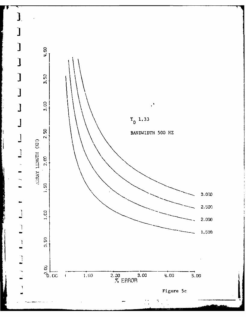
V is the array velocity. In FigLires 3, 4, and 5 we have displayed
the array size necessary for a specified R velocify error at
vertical two way travel times of .133, .333, and 1.333 seconds
bclc- the array for bandwidths of 100, 200, 500 and 1,000 Hz
based on a semblance coefficient of 0.5. (In these plots the
array length calculated from the above formula was doubled to
dcAtcmine the actual array length required.) In Figure 3a we
display the array size necessary for a vertical two way travel
time of .133 second and a bandwidth of 100. To achieve a one_J
percent error in array velocity determination, an array size of
3.9 kl- is required for an array velocity of 2.0 kin/sec. In
F'tu re 3b the bandwidth increases and an array size of about 2.1
:rj is required to achieve the same percent array velocity resolu-
tion. In Figure 3c, where the bandwidth has no.; become 500 liz
it i:; possible to achieve the same array resolution with an array
size of 1.0 kii. In Figure 3d where the baTildwi.dth is 1,000 Iz
]~
I
1-12-
we see that it is possible to achieve the same percent error
I with an array size of approximately 0.6 km. Thus, as the band-
width increases the required spatial. aperture decreases. Clearly
3it is desirable to tow the minimum array length and to have as
broad a bandwidth as possible. However, achievement of the
necessary bandwidth will be restricted by the spectral
characteristics of available sources.J
In Figures 4 and 5 we perform the same analysis but
the time to the reflection horizon is increased. As expected,
when the time to the reflecting horizon beneath the array
Iincreases the required bandwidth and/or the array size must
increai;e to achieve the same accuracy in velocity resolution.
Based on Figure 2, we expect the array velocities to
be between 1.5 and 2.0 km/sec for times of approximately 1 to
1.5 seconds beneath the array corresponding to depths of 500 m
below the sea floor for reasonable intervl velocity functions.
In addition, we ex-,ect that it is pos;ible to obtain source
bandwidths on the order of 200 or possibly even 500 I,. Thi4s
would indicate, based on Figures 3b and c, that an array size
of I km will be adequate for resolving array velocities to within
1one percent for the expected arrival times and for velocities
associated with sedimentary horizons up to 500 m belo%; thc sca
floor. Clearly, if more bandwidth can be obtained and the array
size increased, the resolution will also increase. The bandwidths
we have considered are idealized in the sense that we assume that
all frequencies are equally excited within this band. A bandwidth
L
,Wf l . . .. ... .
f 4] -13-
of 500 Hz actually requires a digitization rate of at least 1,000
]liz, or for a bandwidth of 200 Hz a digitization rate of 400 lHz.
]
-4_S
..S
_5,
-.i
)-14-
II3. Spatial AliasingS]
Spatial aliasing is encountered when the sampling
iinterval in space is too coarse for a given phase velocity
across the array. For example, in Figure 6 we plot frequency
versus wave number and have indicated a phase velocity of
2 km/sec. We have also indicated the Nyquist wave numbers
corresponding to receiver separations of 100, 50, 33 and 25 m.
].Whenever energy is traversing the array at a phase velocity of2 km/sec it will be aliased and appear to lie along the lines
S -J slanting upward to the left. For instance, at 25 m spacing
a 2 km/sec phase velocity is aliased above 40 Hz. This would be
a problem if frequency-wave number processing was to be performed
on the original array data. Usually this is not the case. It
is commnon practice to scan the array arrivals only in a specified
array velocity band since one knows approximately the array
velocities to be determined. Thus, even though the data may be-J
aliased it is often unimportant in practice. If one were to
process the original array data in the frequency-wave number
domain (and were to discriminate based on phase velocity) the
S - alias lines would have to be follow7ed in the manner indicated
in Figure 6.
Dense spatial sampling is required to remove aliasing.
In Figure 6 a spatial sampling interval of 10 m is required to
have unaliased data above 100 11z. Since this necessitates
increasing the number of channels, it becomes difficult to
achieve this type of spatial resolution. The exploration
]-15-
industry is rapidly moving towards longer arrays with denser
]spatial sampling and this has necessitated recording on such mediaas video tape because of the correspondingly high data rates.
]Day to day exploration, however, is cormnonly carried out with
100 or 50 ,n array element spacing intervals. While higher
spatial resolution is clearly desirable, this would increase
]the number of channels and require significantly greater digiti-
zation banchidth than is currently available.
-a
]
I]
"I
!-
t1
t~
-- 16-
- 4. CDP Versus Common Shot Data
Array data is acquired in a Common Shot Point (CSP)
mode, that is, all channels are recorded for a given shot. In
-exploration, this data is reordered into the Common Reflection
Point or Common Depth Point (CDP) mode. CSP and CDP are
equivalent geometries in the case of no dip. In the presence
of dip, however, the CDP geometry has significant advantages.
] Basically this geometry averages the ray -paths such that the
PC'. velocity determined from the array velocity can be used
to give a better indication of the subsurface interval velocities.
Several papers have been written, for example, Shah 1973, which
indicate how array velocity determinations can be turned into
true RMS velocity determinations even in the presence of dip
for the CDP geomIetry. Thus, by measuring the time dip on a
normal incidence record section and using array velocities one
can correct for the presence of dip to improve the interval
velocity determination. In addition, in most cases the effect
of modest dips on the CDP geometry are quite minor. CDP
geometry has a significant advantage over CSP geometry for
horizontally discontinuous or rough reflectors. In the CSP
mode an interface would have to persist laterally for at least
one half the array length in order that true reflections froti
it be recorded on all hydrophone groups. In the CDP mode this
persistance requirement is reduced to the smear in the CDP
caused by errors in the Shot Point placement (navigation) and
reflection dip. This advantage becomes important when attempting
-j
.- 17-
Sto measure IS velocities from rough interfaces such as oceanic
basement, since one need only find a short segment where basement
1is smooth and horizontal. Additionally, after applying moveout
)corrections and stacking the section will be a better representa-
tion of the sub-sea-floor geology in the CDP case.
7To acquire CDP data using a 1 km deep-towed array
with 25 channels and 40 m spacing would require a 20 m shot
Tspacing interval for full 25 fold CDP coverage. If the array
were towed at I kt (.5 m/sec) then a 40 s ec repetition rate
would be required. It would be preferable to tow the array at
2 kt or 1 m/sec and in this case a 20 sec repetition rate would
be required. The CDP mode requires accurate positioning Df the
shot points to avoid smearing the Com,.on Reflection Points
(CrP). For 25 fold data, 25 consecutive shots contribute to
each CDP. It is the average spacing of the shots that must be
controlled accurately, rather than the spacing between individual
shots. For a I km array the 25 shots are spaced over a distance
of 430 m. If one specifies a maximum smear in the CRP's,
caused by misplacement of the shot points, of 5 m, then the
average shot spacing must be accurate to 1 percent. It is
1assumed that longitudinal deformation or stretching of the arraywill be small (i.e. -. 2 nm) If the array is decoupled from the
1source, variations in the distance between the source and the
array must be minimized and known for each shot point. For data
racquired at I kt it would take 1,000 seconds or 16 minutes to
acquire one CDP. Therefore, only slow deformations of the array
would be tolerable. At 2 kts, however, the data would be
TI
.... .-..--.--.--------
I -18-
acquired in 8 minutes and more rapid deformations could be
tolerated.
To acquire CDP data with a deep towed array will
require that kiting be kept to a minimum. The minimum
requirements of 500 Hz bandwidth necessitates that time be
known to less than a millisecond, that is, we must know the
array height to within a meter. In one nreter a pressure
change of 1.5 psi occurs and although an absolute neasurement of
pressure is not necessary, relative pressure and depth should
be recorded to the required accuracy. (An accurate calibration
of the pressure sensing units would be necessary.)
Two corrections are required because of kiting. The
first is a timing correction and the second is a spatial
correction. The array appears smaller as the kiting angle
increases, thus it is absolutely necessary that the array
deformation be known and that this deformation be removed on
a shot basis prior to the CDP gather. Instrumenting the array
with pressure sensors that have been calibrated initially
and have ani accuracy to better than 1.5 psi should provide
sufficient information to remove the effect of kiting. In
* iaddition, if the array is towed with a drogue and the array
is neutrally bouyant and the source and array are mechanically
isolated from the towing cable, the corrections after the initial
settling should he a minimum.
1-19-
] 5. Interval Velocity Error Estimation
In a previous section we discussed array velocity
errors. For relatively small offsets and no dip they can
be considered RMS velocity errors. Here we relate RMS velocity
Ierrors to interval velocity errors.] Interval velocities are calculated from pairs of RIS
velocities and their associated vertical incidence two-way
travel times via Dix's 1955 fnrmula:
V2 &- V,1r V 'eLV
a
P4 r is
W'here V2 and T2 are respectively the 1MS velocity and travel
time to the bottom of the layer, and V aad T refer to the
top of the layer. Each of these terms has an error associated]with it. We know how to calculate RMS velocity errors and we
assume that travel-time to a reflector can be determined to
an accuracy of one source pulse width (i.e. the reciprocal of
the bandwidth). From known errors in Vj. T1 , V and T thereJ c.VI I 2 an 2thr
are several ways to estimate the error intV.ONrJOne could assume that the errors in each of the terms
add algebraically. In this case we would add percent errors
during a mutiplication or division and add actual error for
]additions or subtractions. The square root requires halving
the percent error. This is a form of worst-case error
_J es.imation, since we assume that each term is in error by the
maximum amount and in the most harmful direction.
-20-
A second method assumes that the errors add vectorially.
Instead of adding errors (either percent or actual) we assume
that they are at right angles to each other. Thus an error of
3 percent and an error of 4 percent would yield a combined error
of 5 percent (32 + 42 - 52). This is a form of most probable
error, since we assume that each term will not always be in error
by its maximum amount, that is the errors are independent of each
other.
We have chosen a third methodw\hich is also a form of
worst-case error estimation. First we calculate VMA X by assuming
that V2 is larger than and T is smaller than their true values2 2
by the maximum allowable error. Thus if V is 2,000 m/sec and2
the error estimate is 1 percent we set V2 equal to 2020 m/sec.
Similarly if T is 1.0 second and the error is + 2 milliseconds• 2-
(1/500 liz) then T2 is set to 0.998 seconds. In a similar manner
:e underestimate VI and overestimate TI . This will yield a large
value of VMA, see Figure 7. We then calculate low values for
V2 (1930 m/sec) and TI and high values for V1 and T2 (0.998 sec).
This gives us a low value of V MIN* Then the percent error in V
is estimated as:
j ,ith this type of worst-case crror estimation, the actual errors
t i be less than the estinmted errors. Hlowever, we have pre-
-;cribed error limits and the true interval velocity will. be
.ithin these limits.JAJ
-21-
6. Interval Velocity Resolution
The above discussion gives a proper background to
interpreting Figure 8. In Figure 8 we plot interval velocity
percent error as a function of layer thickness (Delta Z). (It
- must be emphasized at this point that these errors do not include
any error associated with assuming hyperbolic trajectories.)
Figures Ca to e show the interval velocity error as a
function of layer thickness for a I km ar'ray towed 100, 250 and
500 m above the layer for bandwidths of 500 and 200 H1z. The
-- six curves on each plot are for layer velocities from 1,500
m/sec to 2,000 m/sec in 100 m/sec steps. The material above
the layer is assumed to have a velocity of 1,500 m/sec. The most
important feature of these plots is the strong dependance of the
error on array altitude and bandwidth. These empha3ize the need
-- for a large bandwidth source and a low towing altitude. Low
altitude not only achieves higher velocity resolution for thick
beds, but extends this high resolution to thin beds (down to 100 m
in Figure Aa). It appears that 2 percent accuracy can be
achieved with a bandwidth of 500 11z and an altitude of 100 m.
Two other features are evident; the relatively small effect
]interval velocity has on resoltion, and in Figures 8a to 8d
a slight decrease in resolution for thicker beds. This decrease
] in resolution results from flatter hyperbolic trajectories at
the base of the bed as the time to the base increases. This
flattening increases the error in the RMS velocity.
j
-22-
By way of comparison with a surface source and array
we have included similar plots for arrays of 4.8 km and 10 km
length in a water depth of 4 km. (Figures 8f and g) The 10 km
array is hypothetical as we do not know of any in existence.
Note that these two plots have a different thickness axis. For
-J a 1 km thick bed the 4.8 km array has a minimum error of 3 percent
and a 10 km array improves the accuracy to I percent. However,
the velocity error increases rapidly as the bed thickness decreases
below 500 m.
In conclusion we see that interval velocity accuracies
-A near 2 percent can be obtained with a 1 km array towed 100 m
above the sea floor with a source of at least 500 H1z bandwidth.
-44
_ -23-
- 7. Refractions
Critical angle refractions or head waves might be
observed with a 1 km array if it is towed close to the sea floor
and there are shallow high velocity beds. These refractions
- would provide a useful measure of velocity at the top of the
refracting horizon. Refractions normally observed with surface
sonobuoys are generally low frequency which makes it difficult
to accurately measure their arrival time across the array.
The 1 km array coupled with accurate timing could yield good
phase velocity estimates. However, in doing MS velocity
scans it may be necessary to mute or zero the large offset
traces since these arrivals will lead to a degradation in the
FUIS velocities and thus the interval velocity determination.
I1
•
References
Dix, C. w. 1955; Seismic Velocities from Surface Measurements,
Geophysics, Vol. 20, pg. 68 to 86
Shah, Pravin It. 1973; Use of Wavefront Curvature to Relate Seismic
Data with Subsurface Parameters, Geophysics, Vol. 38,
URrAS-VRMSO+( JJ-1 )*rDvRr1S) NEW VRrIS)ER-1DO SO J-.1,NE-; LOOP FOR ALL ERR.ORSI EV-EMIN+(J-1 )*IJCLER- GET ERROR THIS CASETT-TO*TO'( DT*DT)
~1 1 1 T-EV*E:U*TTJ RfADI-TT+0 2Skr)fl-SQRT(RAD1)Pit-D2-RADI+O. 5RO.L12-SORr( RAD2)IX(JER)-VP'1S*DT*-Qtq2/EV, X FROM ED, NO SEM CUADITION YETX(JERq)-XCJEp)/SMIfi; USE SEF1 MIN TO GET REQUIRED PXRRFlY 31Z.ER(JER)EJ#I0; % ERRORIF(>(JER)GT. >WL) GO TO SO
IF(JEk EQ.1) EC-L1., SPVE 1ST ERROR ON PLOTJE~i D-JER.TER-IEP+ I