8

Adaptable PID Versus Smith Predictive Control Applied to an Electric Water Heater System

José António Barros Vieira1 and Alexandre Manuel Mota2 1Polytechnic Institute of Castelo Branco, School of Technology of Castelo Branco,

Department of Electrical and Industrial Engineering, 2University of Aveiro,

Department of Electronics Telecommunications and Informatics, Portugal

1. Introduction

Industry control processes presents many challenging problems, including non-linear or

variable linear dynamic behaviour, variable time delay that means time varying parameters.

One of the alternatives to handle with time delay systems is to use prediction technique to

compensate the negative influence of the time delay. Smith predictor control (SPC) is one of

the simplest and most often used strategies to compensate time delay systems. In this

algorithm it is important to choose the right model representation of the linear/non-linear

system. The model should be accurate and robust for all working points, with a simple

mathematical and transparent representation that makes it interpretable.

This work is based in a previews study made in modelling and controlling a gas water

heater system. The problem was to control the output water temperature even with water

flow, cold water temperature and desired hot water temperature changes. To succeed in this

mission one non-linear model based Smith predictive controller was implemented. The

main study was to identify the best and simple model of the gas water heater system.

It has been shown that many variable industry linear and non-linear processes are

effectively modelled with neural and neuro-fuzzy models like the chemical processes

(Tompson & Kramer, 1994). Hammerstein and Wiener models like pH-neutralization, heat

exchangers and distillation columns (Pottman & Pearson, 1992), (Eskinat et al., 1991). And

hybrid models like heating and cooling processes, fermentation (Psichogios & Ungar, 1992),

solid drying processes (Cubillos et al., 1996) and continues stirred tank reactor (CSTR)

(Abonyi et al., 2002).

In this previews work there were explored this three different modelling types: neuro-fuzzy

(Vieira & Mota, 2003), Hammerstein (Vieira & Mota, 2004) and hybrid (Vieira & Mota, 2005)

and (Vieira & Mota, 2004a) models that reflex the evolution of the knowledge about the first

principles of the system. These kinds of models were used because the system had a non-

linear actuator, time varying linear parameters and varying dead time systems. For dead

time systems some other sophisticated solutions appear like in (Hao, Zouaoui, et al., 2011)

www.intechopen.com

Frontiers of Model Predictive Control 146

that used a neuro-fuzzy compensator based in Smith predictive control to achieved better

results. Or other solutions for unknown dead time delays like (Dong-Na, Guo, et al., 2008)

that use gray predictive adaptive Smith-PID control because the dead time variation is

unknown. There is an interesting solution to control processes with variable time delay

using EPSAC (Extended Prediction Self-Adaptive Control) (Sbarciog, Keyser, et al., 2008)

that could be used in this systems because the delay variations is caused by fluid

transportation.

At the beginning there was no knowledge about the physical model and there were used

black and grey box model approaches. Finally, the physical model was found and a much

simple adaptive model was achieved (the physical model white box modelling).

This chapter presents two different control algorithms to control the output water

temperature in an electric water heater system. The first approach is the adaptive

proportional integral derivative controller and second is the Smith predictive controller

based on the physical model of the system. From the previews work it is known that the first

control approach is not the best algorithm to use in this system, it was used just because it

has a simple mathematical structure and serves to compare results with the Smith predictive

controller results. The Smith predictive controller has a much more complex mathematical

structure because it uses three internal physical models (one inverse and two directs) and

deals with the variable time delay of the system. The knowledge of the physical model

permits varying the linear parameters correctly in time and gives an interpretable model

that facilitate its integration on any control schemes.

This chapter starts, in section 2, with a full description of the implemented system to control

the electric water heater, including a detailed description of the heater and its physical

equations allowing the reader to have a comprehension of the control problems that will be

explained in later sections.

Section 3 and 4, describes the two control algorithms presented: the adaptive proportional

integral derivative control structure and the Smith predictive control based in the physical

models of the heater. These sections show the control results using the two approaches

applied in to a domestic electric water heater system. Finally, in section 5, the conclusions

are presented.

2. The electric water heater

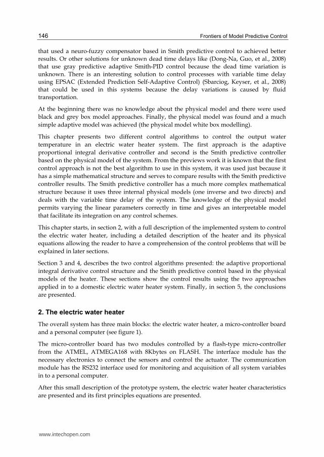
The overall system has three main blocks: the electric water heater, a micro-controller board

and a personal computer (see figure 1).

The micro-controller board has two modules controlled by a flash-type micro-controller

from the ATMEL, ATMEGA168 with 8Kbytes on FLASH. The interface module has the

necessary electronics to connect the sensors and control the actuator. The communication

module has the RS232 interface used for monitoring and acquisition of all system variables

in to a personal computer.

After this small description of the prototype system, the electric water heater characteristics

are presented and its first principles equations are presented.

www.intechopen.com

Adaptable PID Versus Smith Predictive Control Applied to an Electric Water Heater System 147

Fig. 1. System main blocks.

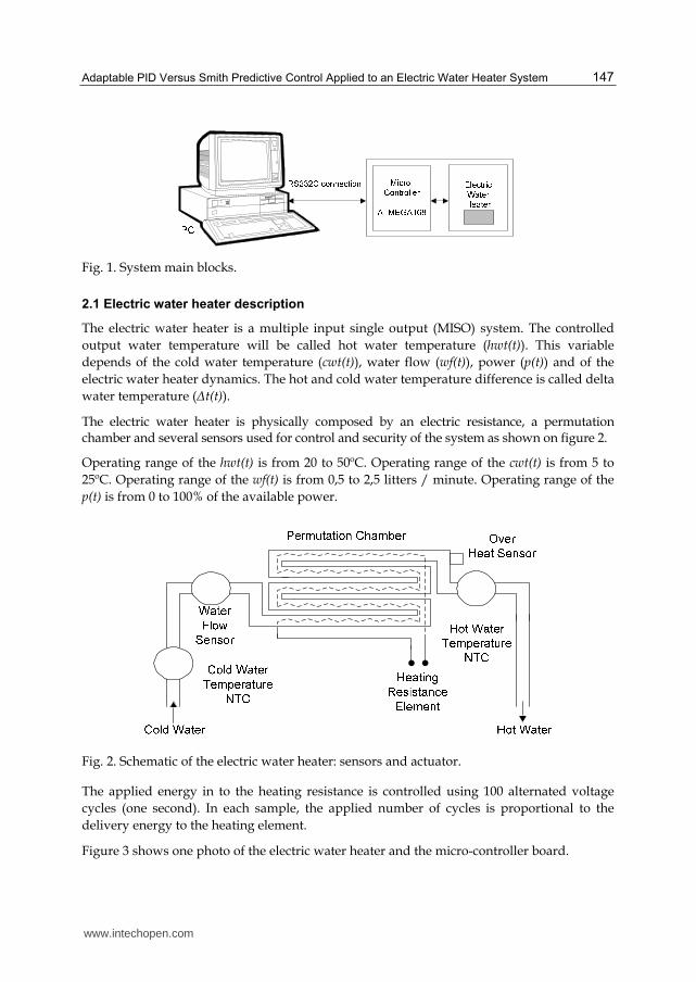
2.1 Electric water heater description

The electric water heater is a multiple input single output (MISO) system. The controlled

output water temperature will be called hot water temperature (hwt(t)). This variable

depends of the cold water temperature (cwt(t)), water flow (wf(t)), power (p(t)) and of the

electric water heater dynamics. The hot and cold water temperature difference is called delta

water temperature (Δt(t)).

The electric water heater is physically composed by an electric resistance, a permutation chamber and several sensors used for control and security of the system as shown on figure 2.

Operating range of the hwt(t) is from 20 to 50ºC. Operating range of the cwt(t) is from 5 to

25ºC. Operating range of the wf(t) is from 0,5 to 2,5 litters / minute. Operating range of the

p(t) is from 0 to 100% of the available power.

Fig. 2. Schematic of the electric water heater: sensors and actuator.

The applied energy in to the heating resistance is controlled using 100 alternated voltage

cycles (one second). In each sample, the applied number of cycles is proportional to the

delivery energy to the heating element.

Figure 3 shows one photo of the electric water heater and the micro-controller board.

www.intechopen.com

Frontiers of Model Predictive Control 148

Fig. 3. Photo of the electric water heater and the micro-controller board.

2.2 Electric water heater first principles equations

Applying the principle of energy conservation in the electric water heater system, equation 1 could be written. This equation was based in a previews work made in modelling a gas water heater system, first time presented in [11].

( )( - ) - ( ) ( ) - ( ) ( )

dEs tQe t td wf t hwt t Ce wf t cwt t Ce

dt (1)

Where dEs(t)/dt=MCe(dΔt(t)/dt) is the energy variation of the system in the instant t, Qe(t) is the calorific absorbed energy, wf(t)cwt(t)Ce is the input water energy that enters in the system, wf(t)hwt(t)Ce is the output water energy that leaves the system, and Ce is the specific heat of the water, M is the water mass inside of the permutation chamber and td is the variable system time delay.

The time delay of the system has two parts: a fixed one that became from the transformation of energy and a variable part that became from the water flow that circulates in the permutation chamber.

M is the mass of water inside of the permutation chamber (measured value of 0,09Kg) and Ce is the specific heat of the water (tabled value of 4186 J/(KgK)). The maximum calorific absorbed energy Qe(t) is proportional to the maximum electric applied power of 5,0 KW.

The absorbed energy Qe(t) is proportional to the applied electric power p(t). On each utilization of the water heater it was considered that cwt(t) is constant, it could change from utilization to utilization, but in each utilization it remains approximately constant. Its dynamics does not affect the dynamics of the output energy variation because its variation is too slow.

Writing equation 1 in to the Laplace domain and considering a fixed water flow wf(t)=Wf and fixed time delay td, it gives equation 2.

www.intechopen.com

Adaptable PID Versus Smith Predictive Control Applied to an Electric Water Heater System 149

1 1

( ) - - ( ) 1

Wf

WfCe WfCe Mt s s td s tde eM WfQe s s sWf M

(2)

Passing to the discrete domain, with a sampling period of h=1 second and with discrete time

delay ( )

( ) int( ) 1td t

d kh

, the final discrete transfer function is illustrated in equation 3.

1( 1) ( ) 1 ( ( ))

Wf Wf

M Mt k e t k e Qe k d kWfCe

(3)

The real discrete time delay 1 2( ) ( ) ( )d k d k d k is given in equation 4, where 1( ) 3d k s is the fixed part of ( )d k that became from the transformation of energy 2( )d k and is the variable part of ( )d k that became from the water flow wf(k) that circulates in the permutation chamber.

4 ( ) 1,75 /min

( ) 5 1,00 /min ( ) 1,75 /min

6 ( ) 1,00 /min

to wf k l

d k to l wf k l

to wf k l

(4)

Considering now the possibility of changes in the water flow, in the discrete domain Wf=wf(k) and ( )2d k , the final transfer function is given in equation 5.

2

2

2

( ( ))

( 1) ( )

( ( ))1

1 ( ( ))( ( ))

wf k d k

Mt k e t k

wf k d k

Me Qe k d kwf k d k Ce

(5)

Observing the real data of the system, the absorbed energy Qe(t) is a linear static function f(.) proportional to the applied electric power p(t) as expressed in equation 6.

( ( )) ( ( ))Qe k d k f p k d k (6)

Finally, the discrete global transfer function is given by equation 7.

2

2

2

( ( ))

( 1) ( )

( ( ))1

1 ( ( ))( ( ))

wf k d k

Mt k e t k

wf k d k

Me f p k d kwf k d k Ce

(7)

www.intechopen.com

Frontiers of Model Predictive Control 150

If A(k) and B(k) are defined as expressed in equation 8, the final discrete transfer function is given as defined in equation 9.

2

2

2

( ( ))

( )

( ( ))1

( ) 1( ( ))

wf k d kMA k e

wf k d kMB k e

wf k d k Ce

(8)

( 1) ( ) ( ) ( ) ( ( ))t k A k t k B k f p k d k (9)

2.3 Physical model validation

For validation of the presented discrete physical model, it is necessary to have open loop

data of the real system. This data has been chosen to respect two important requirements:

frequency and amplitude spectrum wide enough (Psichogios & Ungar, 1992). Respecting the

necessary presupposes, the collect data is made via RS232 connection to the PC. The

validation data and the physical model error are illustrated in figure 4.

Figure 4 shows the physical model error signal e(k), which is equal to the difference between

delta and estimated delta water temperature e(k)= Δt(k)- Δtestimated(k). It can be seen from

this signal, that the proposed model achieved very good results with a mean square error

(MSE) of 1,32ºC2 for the all test set (1 to 1600).

0 200 400 600 800 1000 1200 1400 1600

0

20

40

60

0 200 400 600 800 1000 1200 1400 16000

50

100

0 200 400 600 800 1000 1200 1400 16000

100

200

300

0 200 400 600 800 1000 1200 1400 1600

-5

0

5

Time(seconds)

Fig. 4. Open loop data used to validate the model.

www.intechopen.com

Adaptable PID Versus Smith Predictive Control Applied to an Electric Water Heater System 151

From the validation test, figure 5 shows the two linear variable parameters expressed in equation 8 of the physical model used.

As can be seen the A(k) parameter that multiply with the regressor delta water temperature changes significantly with water flow wf(k) and the B(k) parameter that multiply with the regressor applied power ( ( ))f p k d k presents very small changes with the water flow wf(k).

Fig. 5. The two linear variable parameters A(k) and B(k).

From the results it can be seen that for the small water flows the model presents a bigger error signal. This happens because of the small resolution of the water flow measurements and of the estimated integer time delays forced (a multiple of the sampling time h it is not possible fractional time delays).

3. Adaptive PID controller

The first control loop tested is the adaptive proportional integral derivative control algorithm. Adaptive because we know that gain and time constant of the system changes with the input water flow. First it is described the control structure and its parameters and second the real control results are showed.

3.1 Adaptive PID control structure

This is a very simple and well known control strategy that has two control parameters Kp and Kd that are multiplied by the water flow, as illustrated in figure 6. The applied control signal is expressed in equation 10:

( ) ( 1) ( ) ( )

( ) ( ( ) ( 1))

p

d

f p k f p k wf k K e k

wf k K e k e k

(10)

The P block gives the error proportional contribution, the D block gives the error derivative contribution and the I block gives the control signal integral contribution.

The three control parameters were adjusted after several experimental tests in controlling the real system. This algorithm has some problems dealing with time constant and time delay variations of the system. With this control loop it is not possible to define a close loop

www.intechopen.com

Frontiers of Model Predictive Control 152

Electric

Water

Heater

r(k)+

-

hwt(k)f((p(k))

P

e(k)

wf(k)

+

+

P

I

D

Fig. 6. APID controller constituent blocks.

system with a fixed time constant. The time delay is also a problem that is not solved with this control algorithm.

It was define a reference signal r(t) that is the desired hot water temperature and a water flow wf(t) with several step variations similar to the ones used in real applications. The cold water temperature was almost constant around 13,0 ºC.

For testing the controllers it can be seen that error signal e(t)=r(t)-hwt(t) is around zero excepted in the input transitions. In reference step variations it can be seen that the overshoots for the different water flows are similar but the rise times are clearly different, for small water flows the controller presets bigger rise times. In water flow variations the control loop have some problems because of the variable time delay. This control loop only reacted when error appears.

3.2 Adaptive PID control results

With the proposed tests signals, the tuned adaptive PID control structure was tested in controlling the electric water heater. The APID control results are shown in figure 7.

Fig. 7. Adaptive PID control results.

www.intechopen.com

Adaptable PID Versus Smith Predictive Control Applied to an Electric Water Heater System 153

As it was predicted the results have shown some problems in water flow variations because the controller just reacts when it feels an error signal different from zero.

The evaluation control criterion used is the mean square error (MSE). The MSE in the all test is presented in table 1.

Algorithm MSE Test Set

APID 5,97

Table 1. Mean square errors of the control results.

4. Smith predictive controller

The second control loop tested is the Smith predictive control algorithm. This control strategy is particularly used to control systems with time delay. First it is described the control structure and its parameters and second the control results are showed.

4.1 Smith predictive control structure

The Smith predictive controller is based in the internal model controller architecture that uses the physical model presented in section II, as illustrated in figure 8. It uses two physical direct models one with time delay for the prediction loop and another with out the time delay for the internal model control structure.

Electric Water

Heater

r(k)+

- +

-

Z -1

hwt(k)f(p(k-1))

Physical

Inverse

Modele(k)

cwt(k)

-

-

t(k)-e(k)

Z-d (k)

wf(k-1)Time Delay Function

Physical

Direct

Model

Z -1

Z-d

2 (k)

Filter

Physical

Direct

Model

Fig. 8. SPC constituent blocks.

The Smith predictive control structure has a special configuration, because the systems has two inputs with two deferent time delays so it uses two direct models, one model with time delay for compensate its negative effect and another with out time delay needed for the internal model control structure.

www.intechopen.com

Frontiers of Model Predictive Control 154

The SPC separates the time delay of the plant from time delay of the model, so it is possible

to predict the Δt(k), d(k) ) steps earlier, avoiding the negative effect of the time-delay in the

control results. The time delay is a known function that depends of the water flow wf(k). The

incorrect prediction of the time delay may lead to aggressive control if the time delay is

under estimated or conservative control if the time delay is over estimated (Tan & Nazmul

Karim, 2002), (Tan & Cauwenberghe, 1999).

The physical inverse model is mathematically calculated based in the physical direct model

presented in section 2 used with out time delay.

The low pass filter used in the error feedback loop is a digital first order filter used to filter

the feedback error and indirectly to filter the control signal f(p(k)). The time delay function is

a function of the water flow, which is explained in section 2 and expressed in equation 4.

To test the SPC based in the physical model it was used the same reference signals r(t) and

water flow wf(t) used to test the adaptive PID controller.

4.2 Smith predictive control results

The SPC results are shown in figure 9. As it was predicted from previews work the results

are very good in reference and in water flow changes. The behaviour of the closed loop

system is very similar in every working point.

Fig. 9. SPC control results.

It can be seen that for small water flows the resolution of the measure is small that makes

the control signal a bit aggressive but it does not affect the output hot water temperature.

www.intechopen.com

Adaptable PID Versus Smith Predictive Control Applied to an Electric Water Heater System 155

For small water flows there is another problem with the multiplicity of the time delay and its resolution. With a sampling period of 1 second it is more difficult to use factional time delays that happen in reality. This makes the control results a bit aggressive.

The final MSE evaluation control criterion achieved with the SPC is presented in table 2.

Algorithm MSE Test Set

SPC 3,56

Table 2. Mean square errors of the control results.

The physical model includes à priori knowledge of the real system and has the advantage of been interpretable. This characteristic facilitates the implementation and simplicity the Smith predictive control algorithm.

5. Conclusions

For comparing the two control algorithms, APID and SPC, the reference signals were applied in controlling the system and the respective mean square errors were calculated as showed in table 1 and 2.

This work present and validate the physical model of the electric water heater. This model was based in the model of a gas water heater because of the similarities of both processes.

The MSE of the validation test is very small which validate the physical electric water heater model accuracy.

Finally, the proposed APID and SPC controllers were successful applied in the electric water heater system. It is verify that the SPC achieved much better results than the adaptive proportional integral derivative controller did as it was expected because of the system characteristics.

The best control structure for varying first order systems with varying large time delay is

the Smith predictive controller based in physical model of the system as presented in this

work. The SPC controller proposed in opposition to the APID controller reacts also very

well in cold water temperature variations.

This controller is mathematically simple and easily implemented in a microcontroller with reduce resources.

For future work some improvements should be made as the enlargement of the resolution of

the used water flow and the redefinition of the time delay function.

6. References

Tompson M. L. and Kramer M. A., (1994). Modelling chemical processes using prior knowledge and neural networks, A. I. Ch. E. Journal, 1994, vol. 40(8), pp. 1328-1340.

Pottman M., Pearson R. K., (1998). Block-Oriented NARMAX Models with Output Multiplicities, AIChE Journal, 1998, vol. 44(1), pp. 131-140.

Eskinat E., Johnson S. H. and Luyben W., (1991). Use of Hammerstein Models in Identification of Non-Linear Systems, AIChE Journal, 1991, vol. 37(2), pp. 255-268.

www.intechopen.com

Frontiers of Model Predictive Control 156

Psichogios D. C. and Ungar L. H., (1992). A hybrid neural network-first principles approach to process modelling, AIChE Journal, 1992, vol. 38(10), pp. 1499-1511.

Cubillos F. A., Alvarez P. I., Pinto J. C., Lima E. L., (1996). Hybrid-neural modelling for particulate solid drying processes. Power Thecnology, 1996, vol. 87, pp. 153-160.

Abonyi J., Madar J. and Szeifert F., (2002). Combining First Principles Models and Neural Networks for Generic Model Control, Soft Computing in Industrial Applications - Recent Advances, Eds. R. Roy, M. Koppen, S. O., T. F., F. Homann Springer Engineering Series, 2002, pp.111-122.

Vieira J., Mota A. (2003). Smith Predictor Based Neural-Fuzzy Controller Applied in a Water Gas Heater that Presents a Large Time-Delay and Load Disturbances, Proceedings IEEE International Conference on Control Applications, Istanbul, Turkey, 23 a 25 June 2003, vol. 1, pp. 362-367.

Vieira J., Mota A. (2004). Parameter Estimation of Non-Linear Systems With Hammerstein Models Using Neuro-Fuzzy and Polynomial Approximation Approaches, Proceedings of IEEE-FUZZ International Conference on Fuzzy Systems, Budapest, Hungary, 25 a 29 July 2004, vol. 2, pp. 849-854.

Vieira J., Dias F. and Mota A. (2005). Hybrid Neuro-Fuzzy Network-Priori Knowledge Model in Temperature Control of a Gas Water Heater System, Proceedings of 5th International Conference on Hybrid, Intelligent Systems, Rio de Janeiro, 2005.

Vieira J. and Mota A. (2004a). Water Gas Heater Non-Linear Physical Model: Optimization with Genetic Algorithms. Proceedings of IASTED 23rd International Conference on Modelling, Identification and Control, February 23-25, vol. 1, pp. 122-127.

Psichogios D. C. and Ungar L. H. (1992) A hybrid neural network-first principles approach to process modelling, Journal AIChE, vol. 38(10), pp. 1499-1511.

Tan Y. and Nazmul Karim M. (2002) Smith Predictor Based Neural Controller with Time Delay Estimation. Proceedings of 15th Triennial World Congress, IFAC.

Tan Y. and Van Cauwenberghe A. R. (1999) Neural-network-Based d-step-ahead Predictors for Nonlinear Systems with Time Delay. Engineering Applications of Artificial Intelligence. Vol. 12(1), pp. 21-35.

Hao Chen, Zouaoui, Z. and Zheng Chen (2011) A neuro-fuzzy compensator based Smith predictive control for FOPLDT process. Proceedings of International Conference on Mechatronics and Automation (ICMA), 2011, pp. 1833 – 1838.

Dong-Na Shi, Guo Peng and Teng-Fei Li (2008) Gray predictive adaptive Smith-PID control and its application. Proceedings of International Conference on Machine Learning and Cybernetics, 2008, vol. 4, pp. 1980 – 1984.

M. Sbarciog, R. De Keyser, S. Cristea and C. De Prada (2008) Nonlinear predictive control of processes with variable time delay, A temperature control case study. Proceedings of IEEE Multi-conference on Systems and Control Applications, San Antonio, Texas, USA, September, 2008, pp. 3-5.

www.intechopen.com

Frontiers of Model Predictive ControlEdited by Prof. Tao Zheng

ISBN 978-953-51-0119-2Hard cover, 156 pagesPublisher InTechPublished online 24, February, 2012Published in print edition February, 2012

InTech EuropeUniversity Campus STeP Ri Slavka Krautzeka 83/A 51000 Rijeka, Croatia Phone: +385 (51) 770 447 Fax: +385 (51) 686 166www.intechopen.com

InTech ChinaUnit 405, Office Block, Hotel Equatorial Shanghai No.65, Yan An Road (West), Shanghai, 200040, China

Phone: +86-21-62489820 Fax: +86-21-62489821

Model Predictive Control (MPC) usually refers to a class of control algorithms in which a dynamic processmodel is used to predict and optimize process performance, but it is can also be seen as a term denoting anatural control strategy that matches the human thought form most closely. Half a century after its birth, it hasbeen widely accepted in many engineering fields and has brought much benefit to us. The purpose of the bookis to show the recent advancements of MPC to the readers, both in theory and in engineering. The idea was tooffer guidance to researchers and engineers who are interested in the frontiers of MPC. The examplesprovided in the first part of this exciting collection will help you comprehend some typical boundaries intheoretical research of MPC. In the second part of the book, some excellent applications of MPC in modernengineering field are presented. With the rapid development of modeling and computational technology, webelieve that MPC will remain as energetic in the future.

How to referenceIn order to correctly reference this scholarly work, feel free to copy and paste the following:

José António Barros Vieira and Alexandre Manuel Mota (2012). Adaptable PID Versus Smith Predictive ControlApplied to an Electric Water Heater System, Frontiers of Model Predictive Control, Prof. Tao Zheng (Ed.),ISBN: 978-953-51-0119-2, InTech, Available from: http://www.intechopen.com/books/frontiers-of-model-predictive-control/adaptable-pid-versus-smith-predictive-control-apliyed-to-an-electric-water-heater-system-

© 2012 The Author(s). Licensee IntechOpen. This is an open access articledistributed under the terms of the Creative Commons Attribution 3.0License, which permits unrestricted use, distribution, and reproduction inany medium, provided the original work is properly cited.