Adaptive Antenna Array Processing for GPS Receivers By Yaohua Zheng Thesis submitted for the degree of Master of Engineering Science School of Electrical & Electronic Engineering Faculty of Engineering, Computer & Mathematical Sciences The University of Adelaide Adelaide, South Australia July, 2008
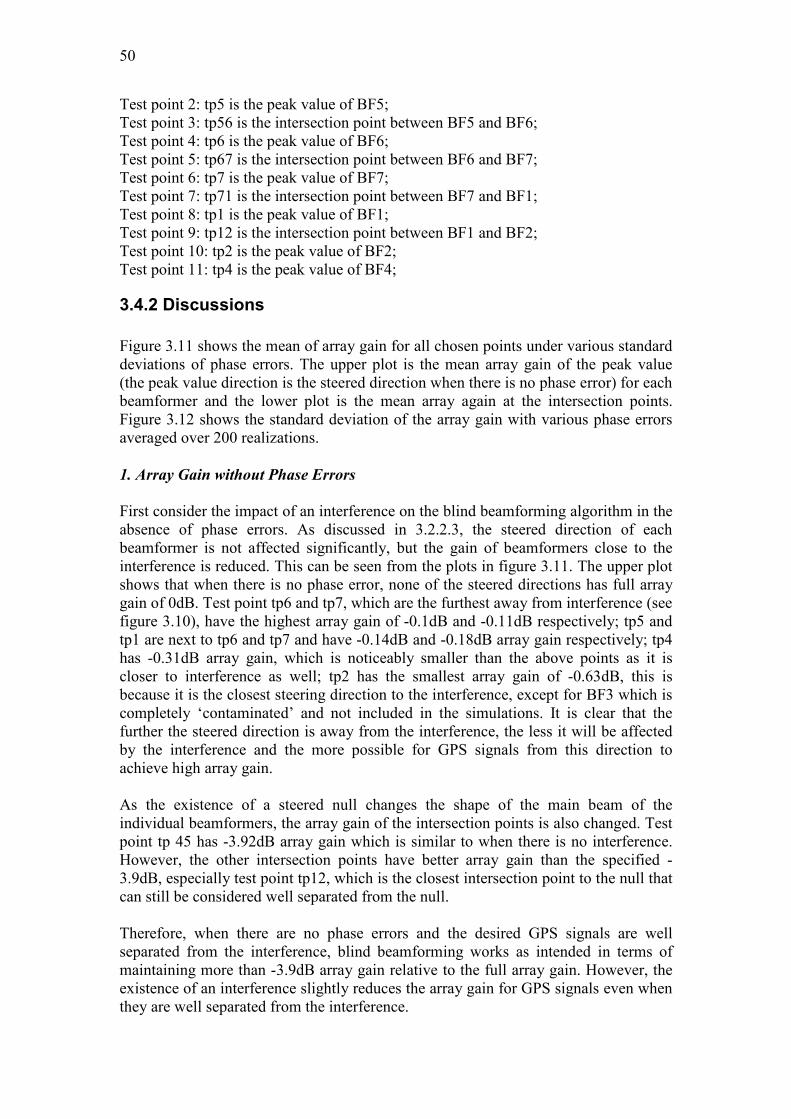
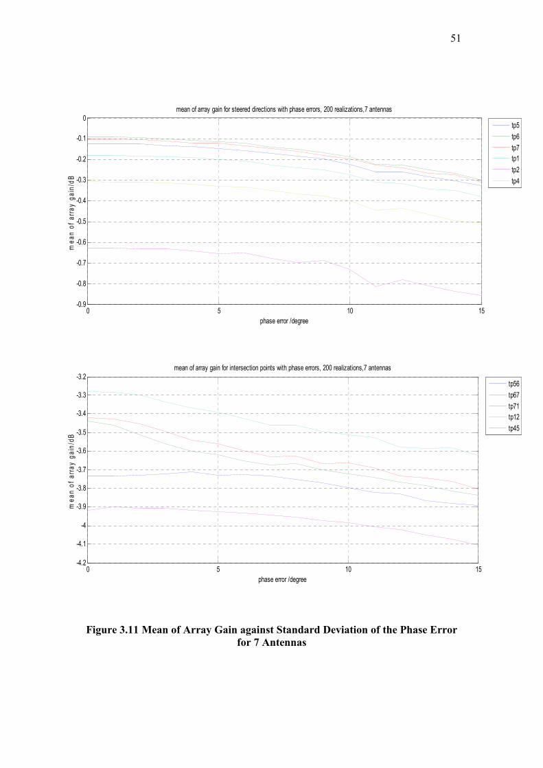
Transcript
Adaptive Antenna Array Processing
for GPS Receivers
By
Yaohua Zheng
Thesis submitted for the degree of
Master of Engineering Science
School of Electrical & Electronic Engineering
Faculty of Engineering, Computer & Mathematical Sciences
The University of Adelaide
Adelaide, South Australia
July, 2008
i
Contents
Statement of Originality ..............................................................................................v
of International Global Navigation Satellite Systems Symposium on GPS/GNSS /
Andrew Dempster (ed.):1-11,Sydney, Australia, 2007.
xvi
1
Chapter 1
Introduction
GPS, the Global Positioning System, was originally designed for the US military in
the 1970s. However, it has been increasingly applied to civilian areas nowadays. GPS
uses one-way ranging from the GPS satellites. Each satellite transmits GPS signals
which are Direct Sequence-Spread Spectrum (DS-SS) modulated with Pseudo-
Random Noise (PRN)* codes. Ranges are measured to four satellites simultaneously
in view by correlating the incoming signal with a user-generated replica signal and
measuring the received phase against the user’s (relatively crude) crystal clock [1].
The time delay )( su tt − for a GPS signal to travel from the satellite to the GPS receiver
is recovered in a special delay lock loop in the GPS receiver, where st is the time
when the GPS signal is transmitted from the satellite and ut is the time when the GPS
signal is received in a receiver. The pseudorange† from the satellite to receiver is
calculated as )( su ttcD −= , where c is the speed of light in space.
1.1 Motivation
The PRN codes used in GPS have low cross-correlation values and enable GPS to use
the Code Division Multiple Access (CDMA) concepts. Because of the use of DS-SS
in the GPS signals, relatively low powers can be transmitted by the satellites and still
be strong enough after correlation to have adequate Carrier power-to-Noise ratio
( 0/ NC )‡ for accurate user localization. However, the low received power makes the
GPS receivers vulnerable to interferences, either intentional or unintentional. As many
new applications have been emerging, some applications exist in environments that
* GPS PRN codes are a subset of a family of Gold codes, including Coarse/Acquisition (C/A) code
and Precision (P/Y) code. More information about the GPS Gold codes can be found on pp 114-118 in
[1].
† As the satellite clock time and user clock time are not accurately synchronized, there is always a
bias in the user’s clock time ut . Therefore the range calculated from )( su ttcD −= is not a “true” range
and is termed “pseudorange”. To solve this problem, another ranging measurement is required from a
fourth satellite to achieve 3-dimension position information.
‡ In this thesis, 0/ NC (dB W/Hz) will be used to describe the power level of GPS signals relative to
background noise, where C stands for the GPS carrier power and No is the noise power density.
2
attenuate the GPS signals to very weak levels. Requirements of such applications are
beyond the capability offered by conventional GPS receivers which motivates
advances in the GPS receiver algorithms. Therefore, the simultaneous suppression of
interferences and enhancement of weak GPS signals are important for GPS
applications.
The GPS receiver’s front end can filter out of band interferences. However, when
interferences occupy the same frequency band, then temporal filtering often can not
be used to separate signals from interferences. Since most interferences in a GPS
operational environment come from directions other than the Direction of Arrival
(DOA) of GPS signals, increasing attention has been paid to applying spatial
processing techniques to protect GPS from various point source interferences.
Adaptive antenna array processing techniques which are also known as adaptive
beamforming operate in the angular or spatial domain and are thus effective against
most point source interferences. Various beamforming algorithms
[11,13,15,23,26,27,28,32,33] have been studied and applied to GPS receivers. Some
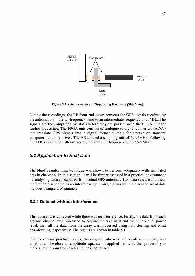
of these algorithms are applied before the correlation stage in GPS receivers, and
others are applied after correlation. A detailed literature review of existing algorithms
applied to GPS will be presented in chapter 2. All of the algorithms referenced in
chapter 2 require some prior information regarding the incoming GPS signals
However, in practice, this prior information is not always available, which leads to the
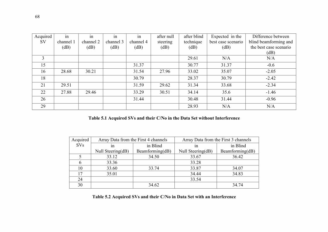
importance of “blind”* beamforming techniques for GPS receivers that require no
GPS signal information. These techniques will be the main focus of this thesis.
1.2 Thesis Outline and Contributions
This thesis proposes a blind beamforming algorithm for GPS receivers. A signal
model is developed in both theory and MATLAB. To compare the performance of
this algorithm with null steering and MMSE algorithm, some simulations were carried
out. Furthermore, this algorithm, together with null steering, was applied to real data.
The thesis is divided as follow:
� Chapter 2 gives the fundamentals of GPS signal and receiver structure and literature review of several existing beamforming techniques, including null
steering, MVDR, MMSE and MaxSINR.
� Chapter 3 describes the proposed blind beamforming technique and gives its simulation results.
Contribution: Proposal of a blind beamforming technique and a MATLAB
model.
* “Blind” here means the algorithm calculates the beamformer weights without knowing a priori
knowledge of the desired signal’s and interferences’ DOA, the Doppler, delays and antenna array’s
manifold. However, the transmitted signal’s waveform is assumed known.
3
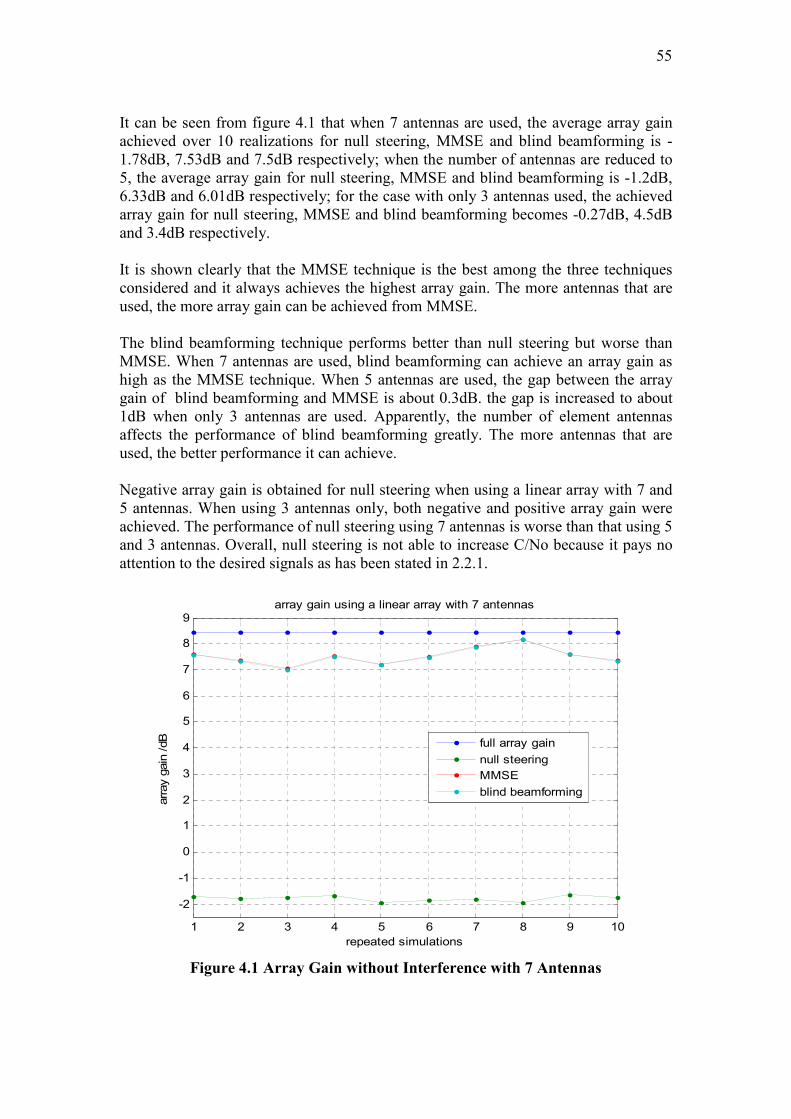
� Chapter 4 compares the blind beamforming technique with null steering and MMSE in various interference environments.
Contribution: Degradation of null steering on GPS signal when there is no
interference present in the received array data is quantified.
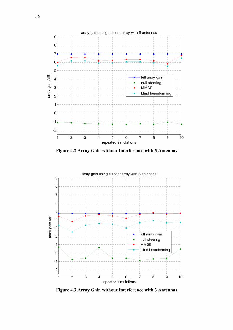
� Chapter 5 analyses the performance of blind beamforming and null steering in two real data sets: one is with an interference in the received data and the other one
with no interference.
Contribution: Application of the blind beamforming technique to real data.
� Chapter 6 summarises the research and draws the conclusions.
4
Chapter 2
Background
This chapter provides some introductory material about GPS and adaptive antenna
array processing used later in this thesis, including the GPS signal structure, the
generic structure of a GPS receiver, interference effects, introduction to beamforming
techniques and a literature review of beamforming algorithms.
2.1 GPS Background Information
2.1.1 GPS Signal Structure
In this section, the fundamentals of GPS signal are introduced, including the
components of a typical GPS C/A signal, the properties of PRN codes and the usual
power level of GPS signal on reception near the Earth’s surface. The characteristics of
the GPS signal structure have a critical impact on the choice of beamforming
algorithms developed for GPS receivers.
2.1.1.1 GPS Signal Components and Generation
Currently, the GPS satellites transmit two types of signals on two carrier frequencies
L1 and L2*. The L1 frequency is 1575.42MHz and the L2 frequency is 1227.6MHz.
The first type of GPS signal is a civilian signal on the L1 carrier frequency, known as
the Coarse/Acquisition (C/A) signal; the other one is a military signal transmitted on
both L1 and L2 carrier frequencies, known as the Precision (P/Y) signal. The use of
L-band as the carrier frequency gives acceptable received signal power and earth
coverage satellite antenna patterns.
Each GPS signal contains three components: an RF carrier frequency, a PRN code
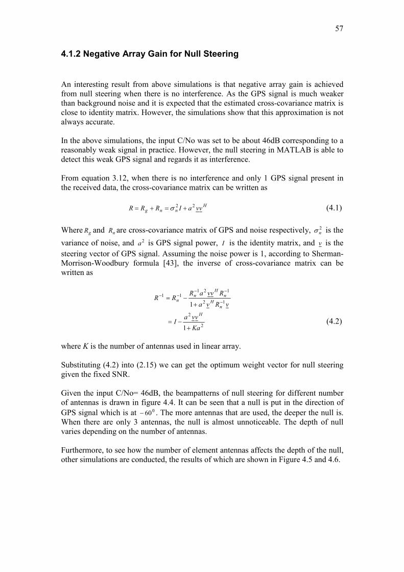
and a navigation message.
* An additional civil signal on the L2 carrier frequency and another two additional civil signals on
the L5 carrier frequency will be transmitted by new GPS satellites in the future. The frequency of L5 is
1176.45MHz [2].
5
The GPS PRN codes are binary codes with values of +1 and -1. For the military
signal, the PRN code used is the P code with a length of 12101871.6 × chips and a
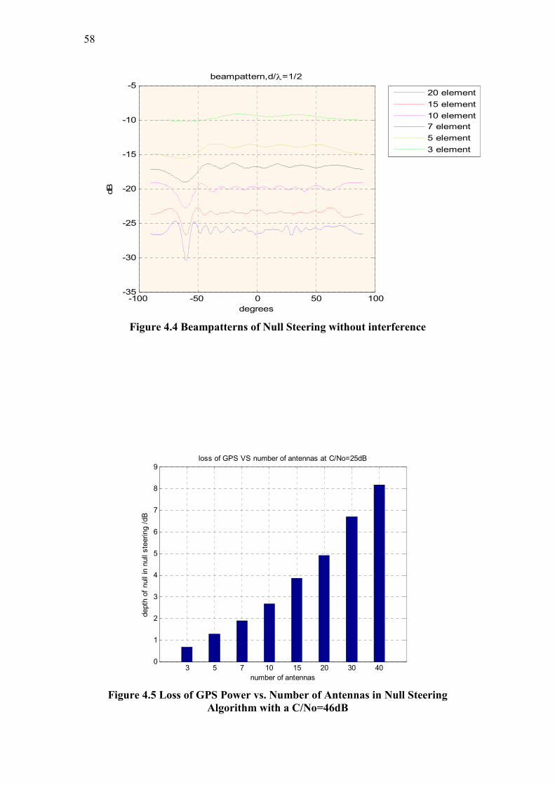
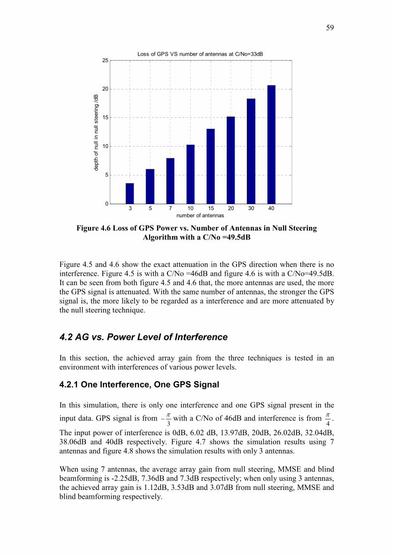
transmission rate of 10.23 Mchip/s. For the civil signal, the PRN code used is the C/A
code with a length of 1023 chips and a transmission rate of 1.023 Mchip/s. GPS C/A
codes with 1 kHz epochs are always available for intended users but civil users do not
have access to the P/Y code when the P/Y code is in the anti-spoof Y-code mode.
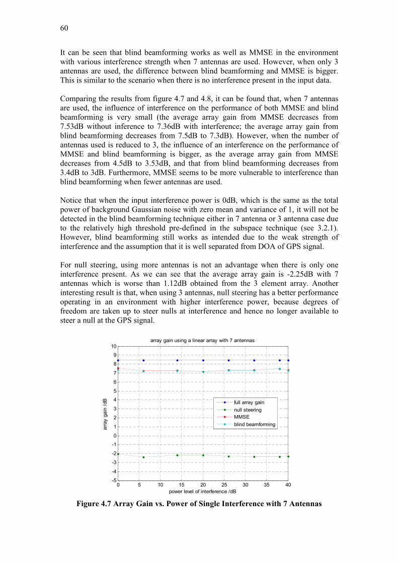
Therefore, only the study of the civil signal modulated with C/A code on the L1
carrier frequency band is considered in this thesis. However, all the techniques,
with suitable modifications, can be extended to P/Y signals.
The navigation message is 50 bps data with the binary values +1 and -1. The
navigation message contains the ephemeris and the almanac data that are needed for
the navigation solution. The data bit is synchronous with the 1 kHz C/A code epochs.
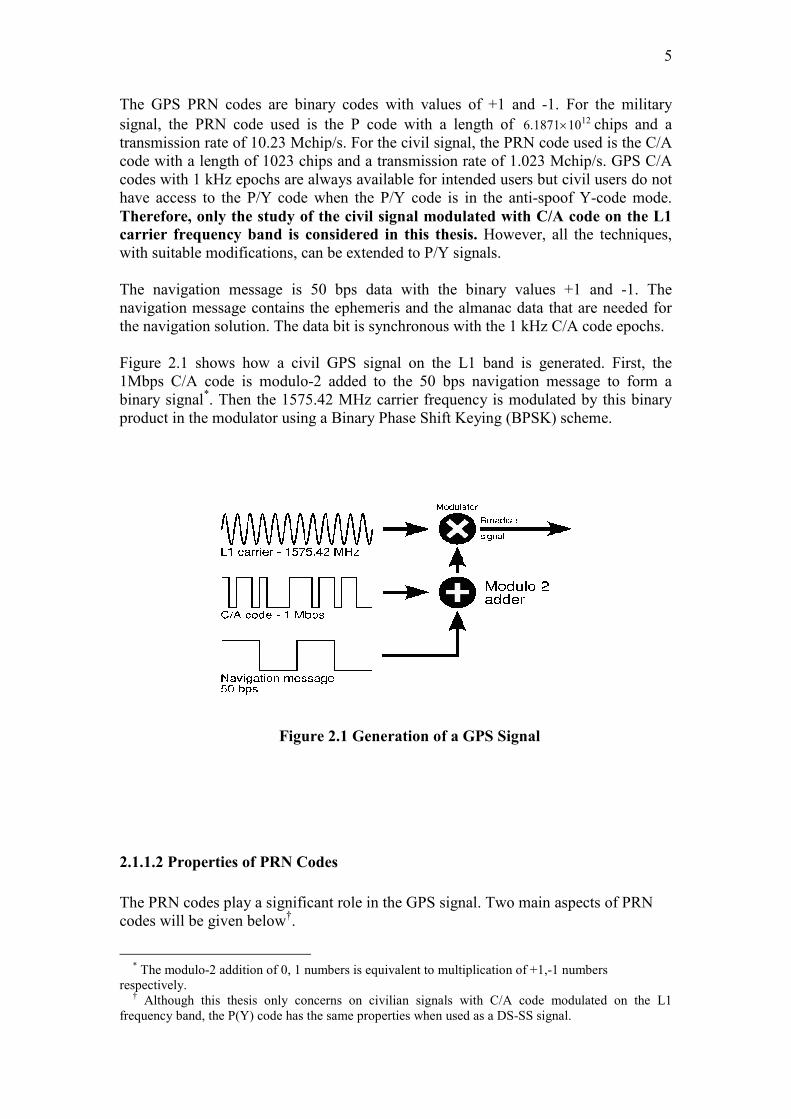
Figure 2.1 shows how a civil GPS signal on the L1 band is generated. First, the
1Mbps C/A code is modulo-2 added to the 50 bps navigation message to form a
binary signal*. Then the 1575.42 MHz carrier frequency is modulated by this binary
product in the modulator using a Binary Phase Shift Keying (BPSK) scheme.
Figure 2.1 Generation of a GPS Signal
2.1.1.2 Properties of PRN Codes
The PRN codes play a significant role in the GPS signal. Two main aspects of PRN
codes will be given below†.
* The modulo-2 addition of 0, 1 numbers is equivalent to multiplication of +1,-1 numbers
respectively.
† Although this thesis only concerns on civilian signals with C/A code modulated on the L1
frequency band, the P(Y) code has the same properties when used as a DS-SS signal.
6
1 The PRN Codes Serve as the Direct Sequence Spread Spectrum Signals (DS-SS)
GPS PRN codes are used as DS-SS signals, also known as Direct Sequence Code
Division Multiple Access (DS-CDMA). Assume the narrow band data signal
)(tD with bandwidth dB is modulated on a sinusoidal carrier to form )(td . When )(td is
multiplied by a PRN code )(tc with bandwidth cB ( dB << cB ), the bandwidth of )(td is
spread to approximately cB . Because the timing of the data and clock transitions are
synchronous, the product )()( tctd has almost exactly the same spectrum as that of
)(tc alone.
The use of DS-SS can also suppress pure tone interferences. Assume the received
signal at a GPS receiver is )()()()()( tntjtctdtr ++= , where )(td and )(tc are the same as
defined above, )(tj is a pure tone interference of power jP and )(tn is additive white
noise of power density 0N . After correlation with an identical and precisely time-
synchronized replica spreading code )(tc , the result
becomes )()()()()()()()()()()()()( 2 tntctjtctdtntctjtctdtctctr ++=++= , because 1)(2 =tc . The
correlation compresses the spread spectrum signal to its original narrow bandwidth
with only the data modulation remaining. Because the GPS PRN code has a
continuous constant envelope, when correlating with white Gaussian noise, the
resulting signal is still white Gaussian noise with same spectral density 0N . However,
the narrow band interference )(tj is now spread by )(tc and has a bandwidth of
approximately cB . Through a bandpass filter with bandwidth of bpB , where bpB is of
the same order as dB , the narrowband signal )(td is passed relatively undistorted and
only a fraction of the noise and interference power passes through the bandpass filter.
The spreading gain from the use of DS-SS is
bp
c
B
B10log10 . For C/A code, cB is
approximately 1MHz and assuming bpB is 20Hz, then the spreading gain is about
47dB.
2 Correlation Properties of C/A Codes
Any GPS receiver must perform a correlation operation if it is to extract the ranging
signal and recover the navigation data. The length of GPS C/A codes is chosen as
1023 in a compromise between fast acquisition and good cross correlation
performance. C/A codes have low cross correlation values. Because of the 1-ms
period of the C/A code, its power spectrum consists of line components spaced at 1
kHz. These line components have approximately, but not exactly, a 2)/(sin xx power
spectral envelope. The power level of the individual line components depends on the
individual code and varies from a worst case of -18.3 to -21.5 dB to more typical
values in the order of -30 dB below the code power for small frequency offsets [1].
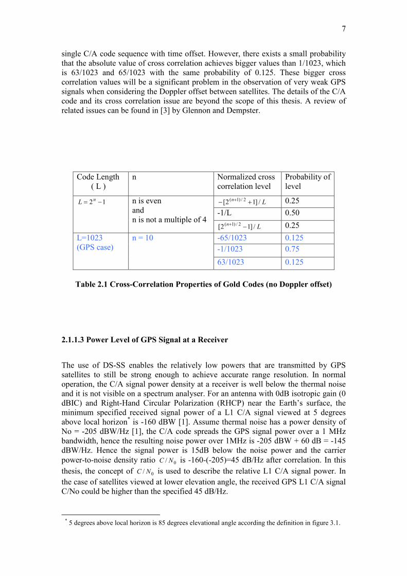
Table 1 shows some cross correlation properties of Gold codes. It can be seen that for
any two different GPS C/A codes with no Doppler offset the cross correlation value is
simply -1/1023 with a probability of 0.75; it is the same for the auto-correlation of a
7
single C/A code sequence with time offset. However, there exists a small probability
that the absolute value of cross correlation achieves bigger values than 1/1023, which
is 63/1023 and 65/1023 with the same probability of 0.125. These bigger cross
correlation values will be a significant problem in the observation of very weak GPS
signals when considering the Doppler offset between satellites. The details of the C/A
code and its cross correlation issue are beyond the scope of this thesis. A review of
related issues can be found in [3] by Glennon and Dempster.
Code Length
( L )
n Normalized cross
correlation level
Probability of
level
Ln /]12[ 2/)1( +− + 0.25
-1/L 0.50
12 −= nL n is even
and
n is not a multiple of 4 L
n/]12[
2/)1( −+ 0.25
-65/1023 0.125
-1/1023 0.75
L=1023
(GPS case)
n = 10
63/1023 0.125
Table 2.1 Cross-Correlation Properties of Gold Codes (no Doppler offset)
2.1.1.3 Power Level of GPS Signal at a Receiver
The use of DS-SS enables the relatively low powers that are transmitted by GPS
satellites to still be strong enough to achieve accurate range resolution. In normal
operation, the C/A signal power density at a receiver is well below the thermal noise
and it is not visible on a spectrum analyser. For an antenna with 0dB isotropic gain (0
dBIC) and Right-Hand Circular Polarization (RHCP) near the Earth’s surface, the
minimum specified received signal power of a L1 C/A signal viewed at 5 degrees
above local horizon* is -160 dBW [1]. Assume thermal noise has a power density of
No = -205 dBW/Hz [1], the C/A code spreads the GPS signal power over a 1 MHz
bandwidth, hence the resulting noise power over 1MHz is -205 dBW + 60 dB = -145
dBW/Hz. Hence the signal power is 15dB below the noise power and the carrier
power-to-noise density ratio 0/ NC is -160-(-205)=45 dB/Hz after correlation. In this
thesis, the concept of 0/ NC is used to describe the relative L1 C/A signal power. In
the case of satellites viewed at lower elevation angle, the received GPS L1 C/A signal
C/No could be higher than the specified 45 dB/Hz.
* 5 degrees above local horizon is 85 degrees elevational angle according the definition in figure 3.1.
8
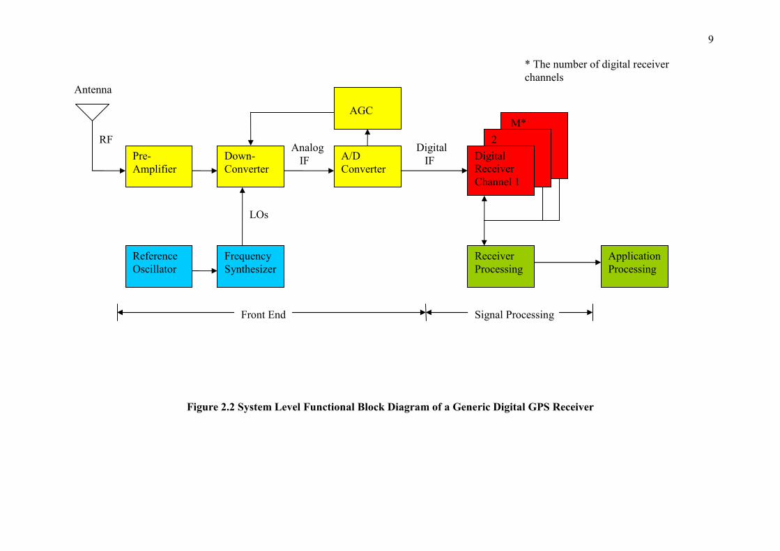
2.1.2 Generic Structure of a Digital GPS Receiver
Most modern GPS receiver designs are digital receivers. This section gives an
introduction to the generic structure of a digital GPS receiver.
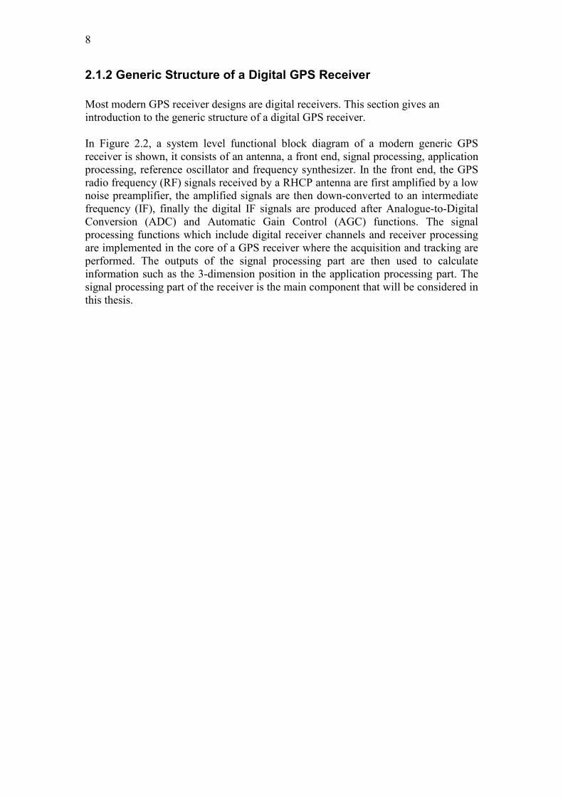
In Figure 2.2, a system level functional block diagram of a modern generic GPS
receiver is shown, it consists of an antenna, a front end, signal processing, application
processing, reference oscillator and frequency synthesizer. In the front end, the GPS
radio frequency (RF) signals received by a RHCP antenna are first amplified by a low
noise preamplifier, the amplified signals are then down-converted to an intermediate
frequency (IF), finally the digital IF signals are produced after Analogue-to-Digital
Conversion (ADC) and Automatic Gain Control (AGC) functions. The signal
processing functions which include digital receiver channels and receiver processing
are implemented in the core of a GPS receiver where the acquisition and tracking are
performed. The outputs of the signal processing part are then used to calculate
information such as the 3-dimension position in the application processing part. The
signal processing part of the receiver is the main component that will be considered in
this thesis.
9
Figure 2.2 System Level Functional Block Diagram of a Generic Digital GPS Receiver
* The number of digital receiver
channels
Signal Processing
Digital
IF
Front End
RF
Antenna
LOs
M*
2 Analog
IF Pre-
Amplifier
Down-
Converter
A/D
Converter
Digital
Receiver
Channel 1
Application
Processing
Reference
Oscillator
Frequency
Synthesizer
AGC
Receiver
Processing
10
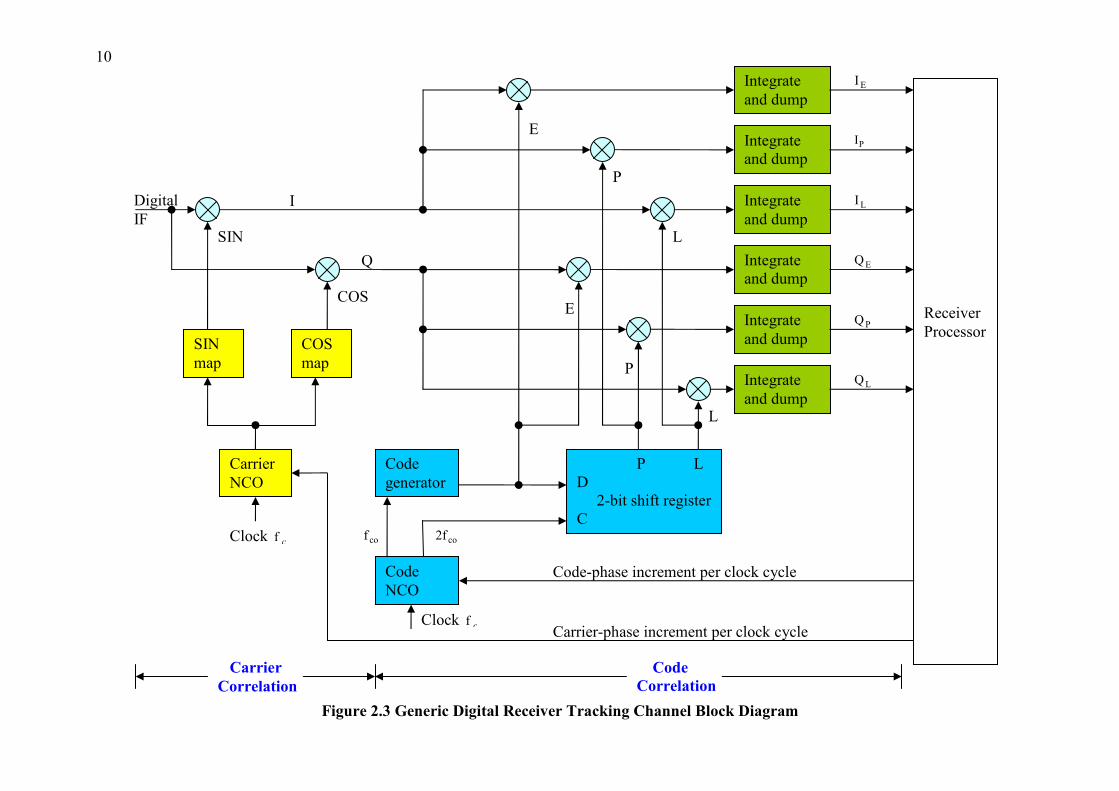
Figure 2.3 Generic Digital Receiver Tracking Channel Block Diagram
Code
Correlation
n
Carrier
Correlation
Clock cf
Code-phase increment per clock cycle
co2f cof
PQ
LQ
EQ
LI
PI
EI
L
L
P
P
E
E
COS
SIN
Q
I Digital
IF
Clock cf
Integrate
and dump
Integrate
and dump
Integrate
and dump
Integrate
and dump
Integrate
and dump
Integrate
and dump
Receiver
Processor SIN
map
COS
map
Carrier
NCO
Code
generator
Code
NCO
P L
D
2-bit shift register
C
Carrier-phase increment per clock cycle
11
2.1.2.1 Acquisition
1. Acquisition
Acquisition is the first step of the GPS signal processing scheme. A GPS receiver
must detect the presence of the GPS signals before they can be tracked and decoded
for positioning computation. The acquisition process must ensure that the signal is
acquired at the correct code phase and carrier frequency [1].
The main purpose of acquisition is to determine the visible Space Vehicles (SVs)*
code and provide a coarse estimate of the Doppler shift and code delay of the acquired
GPS signal which will be used in the tracking stage. The signal acquisition consists of
a two-dimensional search: code phase and frequency. A receiver generates GPS
matching signals with all PRN codes and performs multiple correlations with the
incoming signals. The correlation yields numerous power peaks. Only the main peak
(the largest one) is a valid peak (if there is only one SV present in the data). The
coordinate of the main peak in the frequency search direction indicates its
corresponding Doppler shift and in the code offset direction its code delay.
2. Acquisition Scheme
Various acquisition methods have been developed to acquire the GPS signals [2, 19].
A method called circular correlation by Fourier transforms performs a faster
acquisition over other methods and was used in [17] (the acquisition function used in
the simulation in this thesis is based on the MATLAB acquisition function in [17]).
3 Acquisition Search Band
The satellite motion induces a Doppler shift of up to ±5 kHz from the GPS L1
frequency [20]. The line of sight velocity of the satellite (with respect to the receiver)
causes a Doppler effect resulting in a higher or lower frequency. In most cases it is
sufficient to search the frequencies such that the maximum error will be less than or
equal to 500Hz [21]. Therefore, in the simulations of this thesis, the acquisition search
band was set to be 10± kHz off the IF and search step was set to be 500Hz.
4 Detection Thresholds
The correlation process results in a number of peaks. A threshold signal detector is
required to determine the presence of GPS signals. In [22], the detection threshold is
the minimum value which the correlation peak should exceed for the acquisition
process to declare the signal as acquired. However, in [17], a different detection
scheme was used. That is, after the peak is detected, the second-highest correlation
peak in the same frequency bin as the highest peak is acquired as well, and then the
ratio of the two peaks is used for the signal detection rule. This ratio is compared
* Each SV or satellite has a unique PRN code.
12
against a preset threshold to determine the presence of GPS signals. This preset
threshold is 2.5 in [17] and its MATLAB acquisition function*.
2.1.2.2 Tracking
The main purpose of the tracking channel is to achieve precise Doppler and code
delay. Figure 2.3 shows a high-level block diagram of one of the digital receiver
tracking channels [4].
As can be seen, in carrier correlation, the input digital IF from the front-end is
correlated with the replica carrier signals (SIN and COS map) to produce In-phase (I)
and Quadrature-phase (Q) data. The replica carrier signals are synthesized by the
carrier Numerically Controlled Oscillator (NCO) and the discrete sine and cosine
mapping functions. In code correlation, the I and Q signals are then correlated with
early, prompt and late replica code synthesized by the code generator, a 2-bit shift
register and the code NCO. Normally, the early and late replica codes are 1/2 chip
early and late respectively. When an incoming Space Vehicle (SV) code phase is
tracked correctly, the alignment between prompt replica code phase and incoming SV
code phase produces the highest correlation peak, and the correlation peak between
the early/late replica code phase and the incoming SV code phase is about half the
highest correlation. However, when the code phase is not tracked properly, the
correlations between the replica code phases (early/prompt/late) to the incoming SV
code phase produce different and lower output peaks. Therefore the amount and
direction of the phase change can be detected and adjusted by the code tracking loop
[4].
Notice that the coarse estimate of Doppler and code delay from acquisition is used to
initialise the tracking loop.
2.1.3 RF Interference (RFI)
Any radionavigation system can be disrupted by an interference of sufficiently high
power, and GPS is no exception. As stated in 2.1.1.3, the received GPS signals are
very weak, which makes the system vulnerable to interferences, intentional or
unintentional. Therefore, it is essential to suppress interferences in the signal before it
is further processed. This section introduces some common interferences occurring in
GPS applications and their effects on GPS performance.
* The acquisition detection scheme and MATLAB functions in [17] are adopted in the simulations in
this thesis.
13
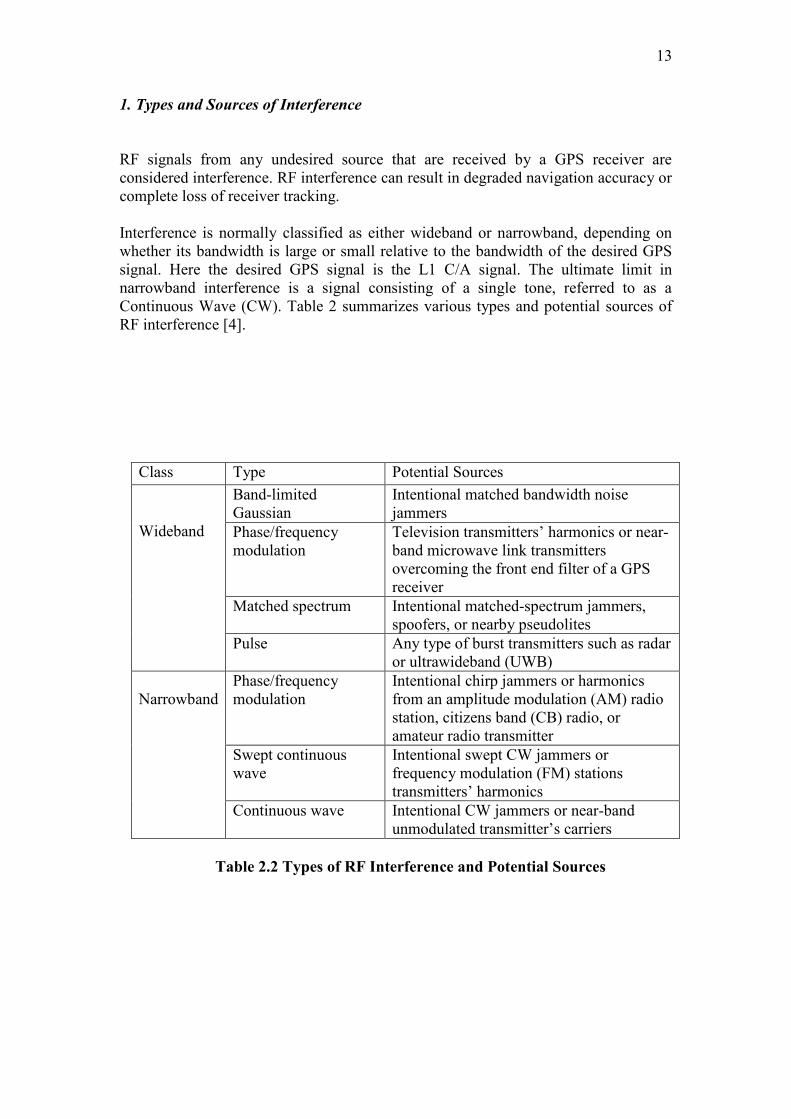
1. Types and Sources of Interference
RF signals from any undesired source that are received by a GPS receiver are
considered interference. RF interference can result in degraded navigation accuracy or
complete loss of receiver tracking.
Interference is normally classified as either wideband or narrowband, depending on
whether its bandwidth is large or small relative to the bandwidth of the desired GPS
signal. Here the desired GPS signal is the L1 C/A signal. The ultimate limit in
narrowband interference is a signal consisting of a single tone, referred to as a
Continuous Wave (CW). Table 2 summarizes various types and potential sources of
Pulse Any type of burst transmitters such as radar
or ultrawideband (UWB)
Phase/frequency
modulation
Intentional chirp jammers or harmonics
from an amplitude modulation (AM) radio
station, citizens band (CB) radio, or
amateur radio transmitter
Swept continuous
wave
Intentional swept CW jammers or
frequency modulation (FM) stations
transmitters’ harmonics
Narrowband
Continuous wave Intentional CW jammers or near-band
unmodulated transmitter’s carriers
Table 2.2 Types of RF Interference and Potential Sources
14
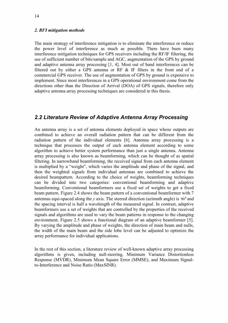
2. RFI mitigation methods
The main strategy of interference mitigation is to eliminate the interference or reduce
the power level of interference as much as possible. There have been many
interference mitigation techniques for GPS receivers including the RF/IF filtering, the
use of sufficient number of bits/sample and AGC, augmentation of the GPS by ground
and adaptive antenna array processing [1, 4]. Most out of band interferences can be
filtered out by either a GPS antenna or RF & IF filters in the front end of a
commercial GPS receiver. The use of augmentation of GPS by ground is expensive to
implement. Since most interferences in a GPS operational environment come from the
directions other than the Direction of Arrival (DOA) of GPS signals, therefore only
adaptive antenna array processing techniques are considered in this thesis.
2.2 Literature Review of Adaptive Antenna Array Processing
An antenna array is a set of antenna elements deployed in space whose outputs are
combined to achieve an overall radiation pattern that can be different from the
radiation pattern of the individual elements [6]. Antenna array processing is a
technique that processes the output of each antenna element according to some
algorithm to achieve better system performance than just a single antenna. Antenna
array processing is also known as beamforming, which can be thought of as spatial
filtering. In narrowband beamforming, the received signal from each antenna element
is multiplied by a “weight”, which varies the amplitude and phase of the signal, and
then the weighted signals from individual antennas are combined to achieve the
desired beampattern. According to the choice of weights, beamforming techniques
can be divided into two categories: conventional beamforming and adaptive
beamforming. Conventional beamformers use a fixed set of weights to get a fixed
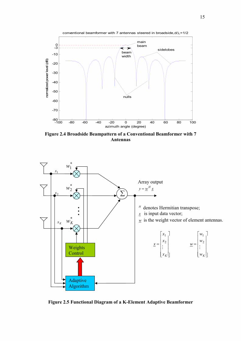
beam pattern. Figure 2.4 shows the beam pattern of a conventional beamformer with 7
antennas equi-spaced along the y axis. The steered direction (azimuth angle) is 090 and
the spacing interval is half a wavelength of the measured signal. In contrast, adaptive
beamformers use a set of weights that are controlled by the properties of the received
signals and algorithms are used to vary the beam patterns in response to the changing
environment. Figure 2.5 shows a functional diagram of an adaptive beamformer [5].
By varying the amplitude and phase of weights, the direction of main beam and nulls,
the width of the main beam and the side lobe level can be adjusted to optimize the
array performance for individual applications.
In the rest of this section, a literature review of well-known adaptive array processing
algorithms is given, including null-steering, Minimum Variance Distortionless
Response (MVDR), Minimum Mean Square Error (MMSE), and Maximum Signal-
to-Interference and Noise Ratio (MaxSINR).
15
-100 -80 -60 -40 -20 0 20 40 60 80 100-80
-70
-60
-50
-40
-30
-20
-10
-30
azimuth angle (degree)
normalized power level (dB)
conventional beamformer with 7 antennas steered in broadside,d/λ=1/2
nulls
sidelobes
main
beam
beam
width
Figure 2.4 Broadside Beampattern of a Conventional Beamformer with 7
Antennas
Figure 2.5 Functional Diagram of a K-Element Adaptive Beamformer
M
Array output
xwyH=
Kx
2x
1x
*Kw
*2w
*1w
∑
Adaptive
Algorithm
Weights
Control
=
Kx
x
x
xM
2
1
=
Kw
w
w
wM
2
1
H denotes Hermitian transpose;
x is input data vector;
w is the weight vector of element antennas.
16
2.2.1 Null Steering
The null steering beamformer is probably the earliest and simplest adaptive
beamforming technique. It was also a variant of the multiple sidelobe cancellers
(MSC), which was developed in the late 1950s by P.Howells [9] and subsequently by
S.Applebaum [10]. The basic idea of null steering is to put the null in the direction of
interference. There are two main techniques depending on how the nulls are steered.
One is based on the priori knowledge of the directions of desired signal and
interference, and the other one is based on the statistics of the received data at the
array.
1 Null Steering with Priori Knowledge
Consider a beamformer with K element antennas which steers a main beam in the
direction of a desired signal and generates L (L<K) nulls in the interference directions.
Assume w is the vector of weights for the beamformer, )(kv is the steering vector
corresponding to the direction k* of the desired signal, )( ikv is the steering vector
corresponding to the direction ik of the thi interference where i=1,2,…L. We want the
summed output of the beamformer to be unity in the direction k of desired signal and
zero in the direction ik of each interference. Then the weight vector w is the solution
to the following simultaneous equations:
1)( =kvwH (2.1)
0)( =iH
kvw i=1, 2 … L (2.2)
Combine equations (2.1) and (2.2) into a single equation:
)1(1+= L
wA δ (2.3)
where A is a KL ×+ )1( matrix given by
=
HL
H
H
kv
kv
kv
A
)(
)(
)(
1
M (2.4)
and )1(1+Lδ is a 1)1( ×+L vector given by
* k is wave vector defined as
=
φφθφθ
λπ
cos
sincos
sinsin2
k , where θ and φ are the azimuth and elevation
angle of GPS signal respectively, and λ is the wave length.
17
=+
0
0
1
)1(1
M
Lδ (2.5)
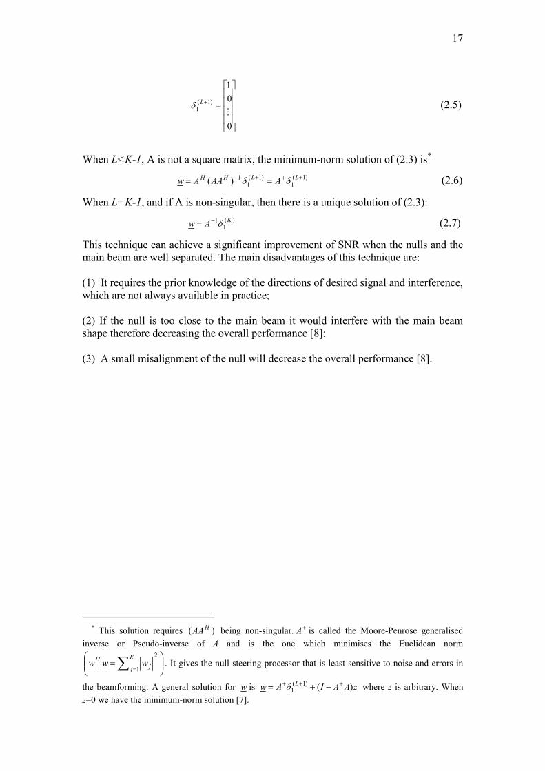
When L<K-1, A is not a square matrix, the minimum-norm solution of (2.3) is*
)1(1
)1(1
1)(+++− == LLHH AAAAw δδ (2.6)
When L=K-1, and if A is non-singular, then there is a unique solution of (2.3):
)(1
1 KAw δ−= (2.7)
This technique can achieve a significant improvement of SNR when the nulls and the
main beam are well separated. The main disadvantages of this technique are:
(1) It requires the prior knowledge of the directions of desired signal and interference,
which are not always available in practice;
(2) If the null is too close to the main beam it would interfere with the main beam
shape therefore decreasing the overall performance [8];
(3) A small misalignment of the null will decrease the overall performance [8].
* This solution requires )( HAA being non-singular. +A is called the Moore-Penrose generalised
inverse or Pseudo-inverse of A and is the one which minimises the Euclidean norm
=∑ =
2
1
K
jj
Hwww . It gives the null-steering processor that is least sensitive to noise and errors in
the beamforming. A general solution for w is zAAIAwL
)()1(
1+++ −+= δ where z is arbitrary. When
z=0 we have the minimum-norm solution [7].
18
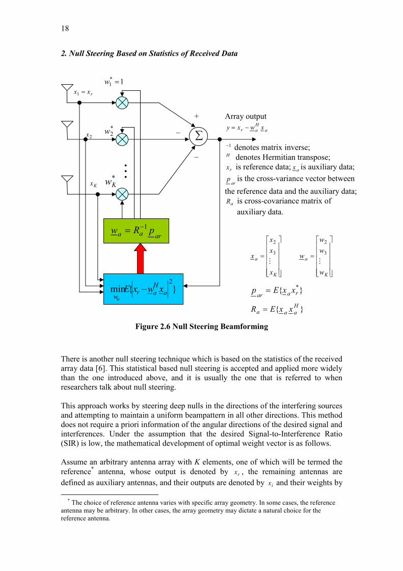
2. Null Steering Based on Statistics of Received Data
Figure 2.6 Null Steering Beamforming
There is another null steering technique which is based on the statistics of the received
array data [6]. This statistical based null steering is accepted and applied more widely
than the one introduced above, and it is usually the one that is referred to when
researchers talk about null steering.
This approach works by steering deep nulls in the directions of the interfering sources
and attempting to maintain a uniform beampattern in all other directions. This method
does not require a priori information of the angular directions of the desired signal and
interferences. Under the assumption that the desired Signal-to-Interference Ratio
(SIR) is low, the mathematical development of optimal weight vector is as follows.
Assume an arbitrary antenna array with K elements, one of which will be termed the
reference* antenna, whose output is denoted by rx , the remaining antennas are
defined as auxiliary antennas, and their outputs are denoted by ix and their weights by
* The choice of reference antenna varies with specific array geometry. In some cases, the reference
antenna may be arbitrary. In other cases, the array geometry may dictate a natural choice for the
reference antenna.
1− denotes matrix inverse; H denotes Hermitian transpose;
rx is reference data; ax is auxiliary data;
arp is the cross-variance vector between
the reference data and the auxiliary data;
aR is cross-covariance matrix of
auxiliary data.
_
_
+ Array output
a
H
ar xwxy −=
Kx
2x
rxx =1
*Kw
M
*2w
1*1 =w
∑
}{min2
a
H
arw
xwxEa
−
araa pRw1−=
=
K
a
x
x
x
xM
3
2
=
K
a
w
w
w
wM
3
2
}{ *raar
xxEp =
}{H
aaa xxER =
19
iw where i =2,…K. For simplicity, all the outputs of the auxiliary antennas are put into
a 1)1( ×−K vector denoted by ax and all their corresponding weights in another
1)1( ×−K vector denoted by aw .The adaptive algorithm is
−
2
min a
H
arw
xwxEa
(2.8)
which is to minimize the mean square error between reference antenna output rx and
the linear combination of auxiliary antennas outputs a
H
a xw , where H denotes the
Hermitian transpose. To achieve the minimum value of equation (2.8) leads to famous
Wiener-Hopf function
araa pwR = (2.9)
The solution of equation (2.9) is
araa
pRw 1−= (2.10)
where, aR is the )1()1( −×− KK co-variance matrix of auxiliary antenna outputs
}{H
aaa xxER = (2.11)
and {}.E denotes the expectation, 1− denotes the matrix inverse. The vector ar
p is the
1)1( ×−K cross-correlation vector between the conjugate of reference antenna output
rx and the auxiliary antenna output vector ax ,
}{ *raar
xxEp = (2.12)
This approach is also called power minimization null steering. Figure 2.6 shows the
block diagram of this approach, where for simplicity, the first antenna is chosen to be
the reference antenna and the remaining antennas make up the auxiliary antennas.
Equation (2.8) can also be interpreted as
{ } wRwwxxwEHHH
w=min subject to 11 =δ
Hw (2.13)
where w is the 1×K vector which includes the weights of all the antenna elements, x
is the 1×K vector consisting of all the antenna element outputs, R is the KK × cross-
covariance matrix of x , and 1δ is a 1×K vector given by
=
0
0
1
1M
δ (2.14)
20
Using the method of Lagrange multipliers, the optimal set of weights is found to be
the solution to
1
11
11
11
1
1
δδ
δ
δδ
δ−
−
−=⇒=
R
Rw
RwR
TngnullsteeriTngnullsteeri (2.15)
The optimal set of weights from a power minimization viewpoint is thus proportional
to the first column of the inverse of the covariance matrix of the array outputs [11].
The advantage of this approach over the null steering with priori knowledge is that the
DOA of the interference needs not be known.
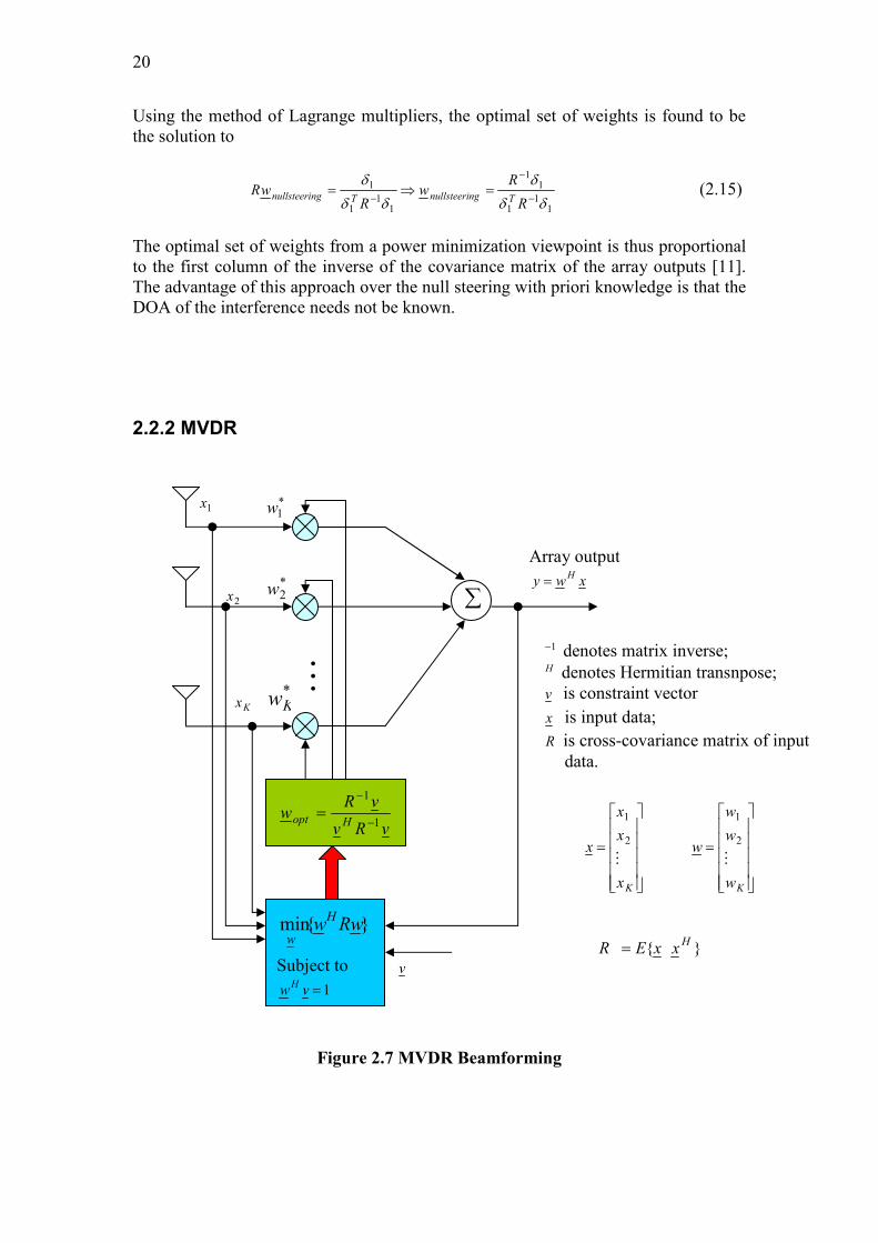
2.2.2 MVDR
Figure 2.7 MVDR Beamforming
v
1− denotes matrix inverse; H denotes Hermitian transnpose;
v is constraint vector
x is input data;
R is cross-covariance matrix of input
data.
Array output
xwyH=
Kx
2x
1x
*Kw
M
*2w
*1w
∑
}{min wRwH
w
Subject to
1=vwH
vRv
vRw
Hopt 1
1
−
−
=
=
Kx
x
x
xM
2
1
=
Kw
w
w
wM
2
1
}{H
xxER =
21
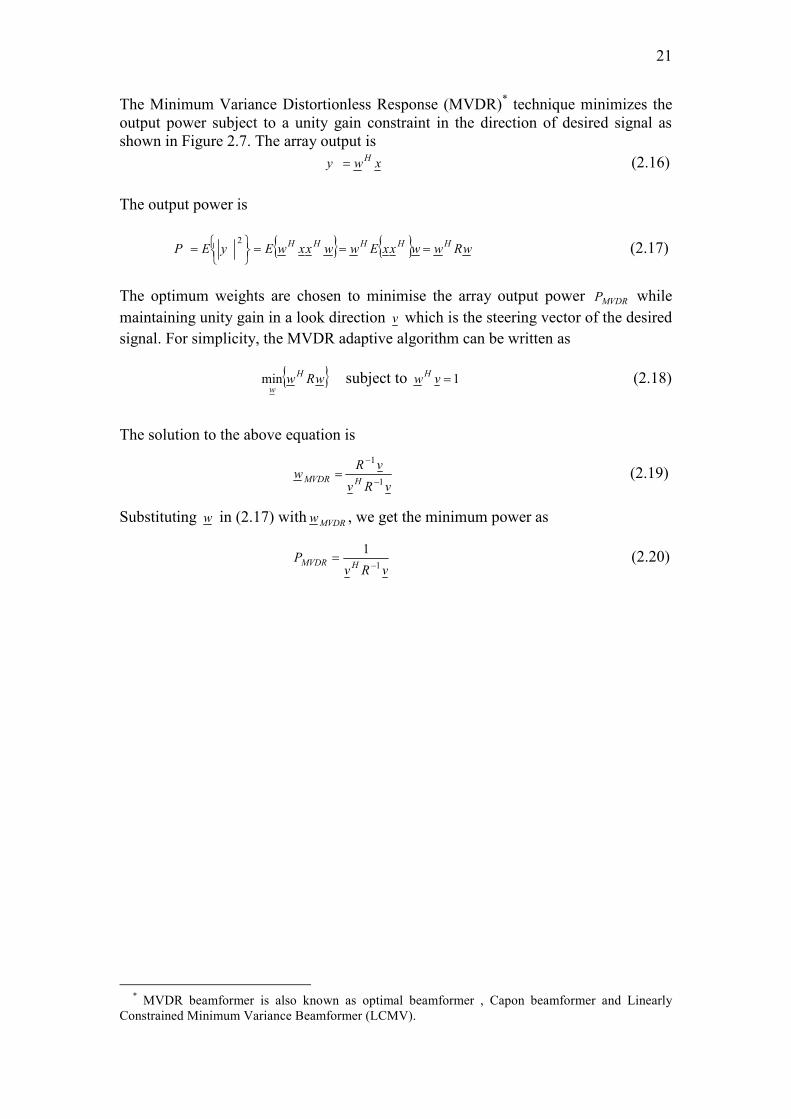
The Minimum Variance Distortionless Response (MVDR)* technique minimizes the
output power subject to a unity gain constraint in the direction of desired signal as
shown in Figure 2.7. The array output is
xwyH= (2.16)
The output power is
{ } { } wRwwxxEwwxxwEyEPHHHHH ===
=
2 (2.17)
The optimum weights are chosen to minimise the array output power MVDRP while
maintaining unity gain in a look direction v which is the steering vector of the desired
signal. For simplicity, the MVDR adaptive algorithm can be written as
{ }wRwH
wmin subject to 1=vw
H (2.18)
The solution to the above equation is
vRv
vRw
HMVDR 1
1
−
−
= (2.19)
Substituting w in (2.17) with MVDRw , we get the minimum power as
vRv
PHMVDR 1
1
−= (2.20)
* MVDR beamformer is also known as optimal beamformer , Capon beamformer and Linearly
Constrained Minimum Variance Beamformer (LCMV).
22
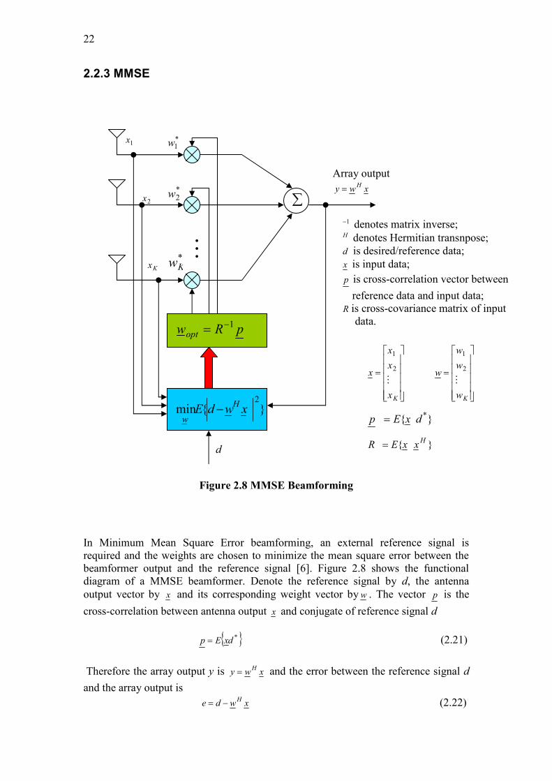
2.2.3 MMSE
Figure 2.8 MMSE Beamforming
In Minimum Mean Square Error beamforming, an external reference signal is
required and the weights are chosen to minimize the mean square error between the
beamformer output and the reference signal [6]. Figure 2.8 shows the functional
diagram of a MMSE beamformer. Denote the reference signal by d, the antenna
output vector by x and its corresponding weight vector by w . The vector p is the
cross-correlation between antenna output x and conjugate of reference signal d
{ }*dxEp = (2.21)
Therefore the array output y is xwyH= and the error between the reference signal d
and the array output is
xwdeH−= (2.22)
d
1− denotes matrix inverse; H denotes Hermitian transnpose;
d is desired/reference data;
x is input data;
p is cross-correlation vector between
reference data and input data;
R is cross-covariance matrix of input
data.
Array output
xwyH=
Kx
2x
1x
*Kw
M
*2w
*1w
∑
}{min2
xwdEH
w−
pRwopt1−=
=
Kx
x
x
xM
2
1
=
Kw
w
w
wM
2
1
}{ *dxEp =
}{H
xxER =
23
The MMSE criterion is
{ }
−=
22minmin xwdEeE
H
ww (2.23)
The optimal Wiener-Hopf solution for the weight vector w is
pRw1−= (2.24)
2.2.4 MaxSINR
Figure 2.9 MaxSINR Beamforming
As indicated by its name, MaxSINR choses the weights to directly maximize the
signal-to-interference plus noise ratio [6,23,24]. This algorithm is described in figure
2.9. Assuming the output vector of the antennas x includes the desired signals,
1− denotes matrix inverse; H denotes Hermitian transnpose;
R is cross-covariance matrix of input
Data;
maxλ is maximum eigenvalue of R
dR is cross-covariance matrix of desired
signal;
nR is cross-covariance matrix of
interference and noise
Array output
xwyH=
Kx
2x
1x
*Kw
M
*2w
*1w
∑
wRw
wRw
inH
dH
wmax
optoptsn wwRR max1 λ=−
=
Kx
x
x
xM
2
1
=
Kw
w
w
wM
2
1
}{H
xxER =
24
interference and Gaussian noise that are mutually uncorrelated, then the overall cross
covariance matrix is
{ } indnidH
RRRRRxxER +=++== (2.25)
where dR is the cross covariance matrix of the desired signals and inR is the cross
covariance matrix of interference plus Gaussian noise. Consequently, the output
desired signal power is
wRwP dH
d = (2.26)
and the output interference plus Gaussian noise power is
wRwP inH
in = (2.27)
The output SINR is therefore written as
wRw
wRw
P
PSINR
inH
dH
in
d == (2.28)
The solution to equation (2.28) results in the following eigenvalue equation [5]
wRwRP
PwR in
P
P
inin
dd
in
d
λ
λ
==
=
wwRR din λ=⇒ − )( 1 (2.29)
where λ and w are the eigenvalue and corresponding eigenvector of the
matrix )( 1din RR − . Obviously, the maximization of equation (2.28) is the maximum
eigenvalue in equation (2.29), that is, maxmax λ=SINR .
The optimum weight vector of the array is therefore the eigenvector corresponding to
maxλ , that is
optoptdin wwRR max1
)( λ=− (2.30)
As the cross covariance matrix dR of desired signals is hard to obtain but the overall
cross covariance matrix R of received data is easier to obtain, the maximization of
equation (2.28) can be rewritten as
1max)(
maxmaxmaxmax −=−+
===wRw
wRw
wRw
wRRRw
wRw
wRw
P
PSINR
inH
H
win
H
inindH
win
H
dH
win
d (2.31)
The solution to equation (2.31) becomes
optoptin wwRR max1)( λ=− (2.32)
25
Here maxλ and optw are the eigenvalue and corresponding eigenvector of the matrix
)( 1RRin− .
To solve equation (2.32), we only need to know R and inR and then to solve the
generalised eigen value problem for the weights. For the GPS case, it is possible to
separate inR from R . That is, when the SVs are successfully acquired by the
acquisition procedure, we purposefully mis-align either the code delay or carrier
frequency in the GPS tracking loops (see Figure 2.3) to remove GPS signals and thus
obtain interference plus noise cross covariance matrix.
2.2.5 Sampled Matrix Inversion
The optimal solutions introduced in the above four sections require the exact cross-
covariance matrix R in time domain. However, the exact R is not always available in
practice which leads to the estimation and adaptation techniques of the exact R.
The Least Mean Square (LMS) [37, 38] algorithm is a well-known and simple linear
adaptive filtering algorithm. It makes use of the estimates of the gradient vector from
the data, performs an iterative procedure to adjust the weight vector successively and
eventually leads to the least mean square error. However, it has slow convergence
when the eigenvalues of the covariance matrix are widespread [39]. Sample Matrix
Inversion (SMI) [7,39,40] is another interesting algorithm to estimate and update the
cross-covariance matrix. This technique assumes that consecutive data from the array
antennas is independent and ergodic, which is reasonable for GPS application. SMI
has a faster convergence than LMS since it employs matrix inversion directly but also
has higher computational complexity. The SMI technique is used to estimate the
cross-covariance matrix in the simulations associated with this thesis.
2.3 Application of Adaptive Array Processing to GPS
The desired GPS signals are 20dB to 30dB below the noise floor [31]. Consequently,
all signals above noise floor may be considered as interference, or jamming sources
[34]. Due to this property, the statistics based null steering technique is widely applied
to GPS. In [11], this technique is also called power minimization approach. It is a
simple real-time adaptive function based on equation (2.8). That is, the reference
antenna output may be viewed as a “reference signal” and the output of the linear
combination from the auxiliary elements as an estimate of the “desired signal”
leading to a simple LMS or RLS based algorithm for adapting the weights on a
continual basis [11]. Also it can effectively cancel up to (K-1) point source
interferences. The performance of such a technique was tested on a UAV by Li in
[12]. In [13, 14], the polarization information was exploited when implementing the
null steering algorithm. In [31], this technique is applied in a circular array. However,
the disadvantages of statistics based null steering are obvious. It can only be applied
26
in the case where the desired signal is much less than noise power or absent from the
auxiliary antennas. Another significant shortcoming of the approach is that since there
is no look direction constraint imposed on the optimum weights, it pays no attention
to the desired GPS signal, therefore there is no guaranteed preservation of GPS
signals. Apart from the viewpoint of preservation of GPS signal, when there is no
interference, the auxiliary weights will be zero and no array gain will be achieved.
The MVDR algorithm has also been applied to GPS. MVDR works well if a look
direction is given. It makes best use of available degrees of freedom to shape the
spatial nulls and has a greater probability to preserve GPS signals compared to null
steering [36]. However, in most practical situations, the direction of an incoming GPS
signal relative to the array coordinate system is usually unknown. Furthermore, when
the assumed steering vector doesn’t exactly coincide with actual steering vector for an
incoming desired signal, the performance of MVDR degrades as the desired signal is
viewed as interference [11]. The degradation varies with the extent of mismatch.
When applying the MMSE algorithm to GPS, the biggest change is to find the
reference signal. As for the GPS case, it is impossible to achieve a reference signal
before acquisition and tracking stage. However, once a GPS signal is tracked, a
reference signal can be derived from the code and tracking loops and therefore the
Least Mean Square (LMS) approach can be implemented to optimise this criterion. In
[15], Lorenzo et al. compared the LMS approach with other techniques such as
conventional beamforming and Applebaum beamforming. It was shown that the LMS
based approach had significant advantages in an environment where there are various
errors present such as antenna array phase-centre errors, RF front-end effects and RF
interference effects.
MaxSINR has other derivatives, such as maximum signal-to-noise ratio (maxSNR)
and maximum signal-plus-noise-to-noise ratio (MSNNR). However, all of these
involve solving the problem of separating the cross-covariance matrix of the desired
GPS signal from the cross-covariance of the interference or overall cross-covariance
matrix. Before the correlation procedure, the GPS signal is buried in background
noise and it is difficult to separate the GPS signal from noise and interference.
Therefore, maxSINR algorithm is usually combined with correlation processing. Lin
used the subspace approach (similar to the method introduced in 3.2.1) to remove
strong interferences from the input data and then applied the MSNNR algorithm for
remaining signals which are assumed to be GPS signals in [27], it is a completely
blind technique that does not require correlation processing. However, this technique
only forms one beam to maximise the SNR for all GPS signals and not much array
gain will be achieved with a limited number of antennas in an array when there are
many GPS signals (usually more than 4). In [25], the maxSINR described in equation
2.31 is applied and the matched filter method was used to classify/estimate overall
cross-covariance and interference plus noise cross-covariance. It is a blind adaptive
algorithm requiring no DOAs of desired signals or interference or array manifold by
exploiting the Doppler diversity and delay diversity amongst the desired signal and
interferences, but it requires the GPS signal code phase & carrier frequency for the
correlation processing. A very good review of adaptive techniques applied to DS-SS
multiple-access systems is given in [24] and a linear structure combining a
conventional matched filter and a tapped delay line is proposed. This technique has
27
unified capability of rejecting narrowband interferences and multipath components
when the maxSNR algorithm is applied. It gives the theoretical improvements and
limits that adaptive algorithms including maxSNR and MMSE can achieve.
Furthermore, an iterative blind adaptation is proposed in [35] to improve the method
introduced in [24] and it demonstrates faster convergence time.
2.4 Summary
This chapter begins with the fundamentals of GPS signal and GPS receivers, and then
demonstrates the potential RFI resources and several existing interference mitigation
methods. Lastly, a literature review of several adaptive array processing
(beamforming) techniques and their applications to GPS is presented. The study on
advantages and disadvantages of those beamforming techniques leads to a potential
improved beamforming technique—blind beamforming, which will be described in
next chapter.
28
Chapter 3
A Blind Beamforming Technique for GPS Receivers
Adaptive beamforming is an effective spatial signal processing technique to reject
interferences when the DOA’s are different to those of the desired GPS signals. As
stated in 2.2, commonly used adaptive array processing algorithms are most effective
in the case of GPS only when at least one prior information is given, either the DOA
of GPS signal (MVDR) or code phase (MMSE). However, in practice, this prior
information of the GPS signals is not always available. This has motivated the study
of GPS beamforming techniques operating in a ‘blind’ environment. This chapter
presents a blind beamforming technique for GPS receivers under the assumption that
GPS signal are spatially well separated from the interference. First, a signal model for
this technique is built; then more details of this technique are illustrated; finally a
simulation model is carried out and the results are discussed.
3.1 Signal Model
1 Assumption and Definitions
As mentioned before, this thesis only considers the GPS L1 C/A code signal which is
in the microwave frequency range, hence it is reasonable to assume that GPS signals
propagate in straight lines. Interferences here are considered to be wideband* FM
interferences modulated on the same carrier frequency band as the GPS L1 signals
and well separated from GPS signals through the whole thesis.
Furthermore, the following assumptions regarding the antenna elements are made
throughout the whole thesis:
(1) All antennas are considered immersed in a field which is comprised of the
superposition of waves propagating through free space. The antennas convert the
signals to electrical signals that are then processed;
* Notice the bandwidth of wideband FM interferences here is about 1MHz, similar to that of C/A
codes. It is ‘wide’ compared to C/A code, however, it is considered narrowband compared to L1 carrier
frequency.
29
(2) The antennas are sufficiently distant from the sources such that the waves can be
treated as plane;
(3) Each antenna is ‘transparent’ and that its presence does not affect the signals at
arriving at any other receiver of the array, i.e. mutual coupling is ignored;
(4) Each antenna element is considered to be a point receiver at given spatial
coordinate and all the antennas are considered to be identical.
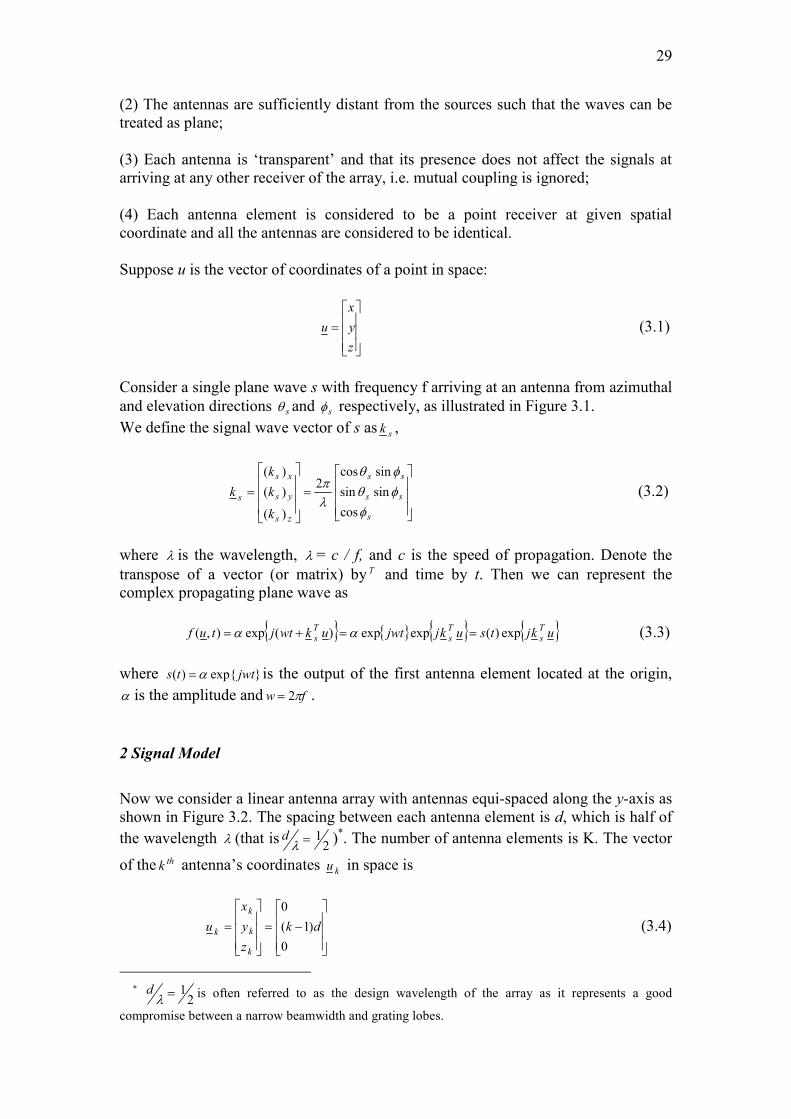
Suppose u is the vector of coordinates of a point in space:
=
z
y
x
u (3.1)
Consider a single plane wave s with frequency f arriving at an antenna from azimuthal
and elevation directions sθ and sφ respectively, as illustrated in Figure 3.1.
We define the signal wave vector of s as sk ,
=
=
s
ss
ss
zs
ys
xs
s
k
k
k
k
φ
φθ
φθ
λπ
cos
sinsin
sincos2
)(
)(
)(
(3.2)
where λ is the wavelength, λ = c / f, and c is the speed of propagation. Denote the transpose of a vector (or matrix) by T and time by t. Then we can represent the
complex propagating plane wave as
{ } { } { } { }ukjtsukjjwtukwtjtufT
s
T
s
T
s exp)(expexp)(exp),( ==+= αα (3.3)
where }exp{)( jwtts α= is the output of the first antenna element located at the origin,
α is the amplitude and fw π2= .
2 Signal Model
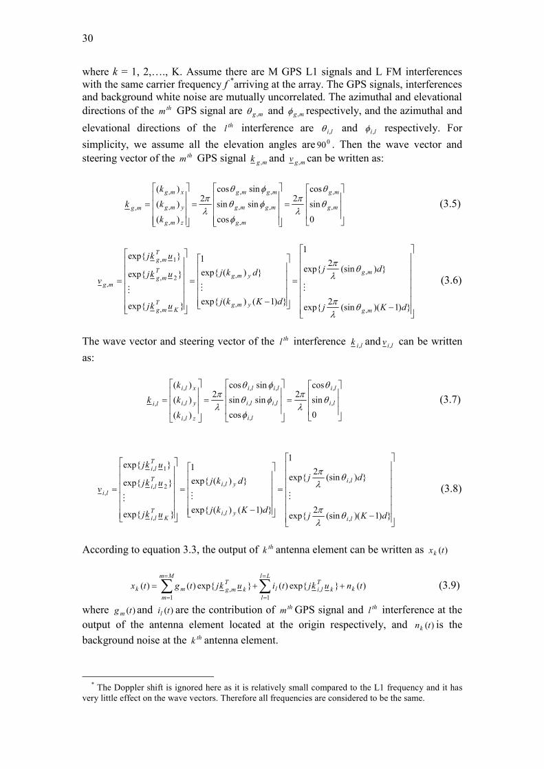
Now we consider a linear antenna array with antennas equi-spaced along the y-axis as
shown in Figure 3.2. The spacing between each antenna element is d, which is half of
the wavelength λ (that is21=λ
d )*. The number of antenna elements is K. The vector
of the thk antenna’s coordinates ku in space is
−=
=
0
)1(
0
dk
z
y
x
u
k
k
k
k (3.4)
*
21=λ
d is often referred to as the design wavelength of the array as it represents a good
compromise between a narrow beamwidth and grating lobes.
30
where k = 1, 2,…., K. Assume there are M GPS L1 signals and L FM interferences
with the same carrier frequency f *arriving at the array. The GPS signals, interferences
and background white noise are mutually uncorrelated. The azimuthal and elevational
directions of the thm GPS signal are mg ,θ and mg ,φ respectively, and the azimuthal and
elevational directions of the thl interference are li,θ and li,φ respectively. For
simplicity, we assume all the elevation angles are 090 . Then the wave vector and
steering vector of the thm GPS signal mgk , and mgv , can be written as:
=
=
=
0
sin
cos2
cos
sinsin
sincos2
)(
)(
)(
,
,
,
,,
,,
,
,
,
, mg
mg
mg
mgmg
mgmg
zmg
ymg
xmg
mg
k
k
k
k θ
θ
λπ
φ
φθ
φθ
λπ
(3.5)
−
=
−
=
=
})1)((sin2
exp{
})(sin2
exp{
1
})1()(exp{
})(exp{
1
}exp{
}exp{
}exp{
,
,
,
,
,
2,
1,
,
dKj
dj
dKkj
dkj
ukj
ukj
ukj
v
mg
mg
ymg
ymg
K
T
mg
T
mg
T
mg
mg
θλπ
θλπ
MMM
(3.6)
The wave vector and steering vector of the thl interference lik , and liv , can be written
as:
=
=
=
0
sin
cos2
cos
sinsin
sincos2
)(
)(
)(
,
,
,
,,
,,
,
,
,
, li
li
li
lili
lili
zli
yli
xli
li
k
k
k
k θ
θ
λπ
φ
φθ
φθ
λπ
(3.7)
−
=
−
=
=
})1)((sin2
exp{
})(sin2
exp{
1
})1()(exp{
})(exp{
1
}exp{
}exp{
}exp{
,
,
,
,
,
2,
1,
,
dKj
dj
dKkj
dkj
ukj
ukj
ukj
v
li
li
yli
yli
K
T
li
T
li
T
li
li
θλπ
θλπ
MMM
(3.8)
According to equation 3.3, the output of thk antenna element can be written as )(txk
)(}exp{)(}exp{)()(
1
,
1
, tnukjtiukjtgtx k
Ll
l
k
T
lil
Mm
m
k
T
mgmk ++= ∑∑=
=
=
=
(3.9)
where )(tgm and )(til are the contribution of thm GPS signal and thl interference at the
output of the antenna element located at the origin respectively, and )(tnk is the
background noise at the thk antenna element.
* The Doppler shift is ignored here as it is relatively small compared to the L1 frequency and it has
very little effect on the wave vectors. Therefore all frequencies are considered to be the same.
31
Figure 3.1 Coordinate System
Figure 3.2 A Linear Array with Antennas Equi-spaced along y Axis
Incoming plane
waves
x
z
y antenna
θ
φ
θ
(M-1)d 2d d 0
Element
M
3 2 Element
1
32
Denoting the outputs of the antennas in a vector form
=
)(
)(
)(
)(2
1
tx
tx
tx
tx
K
M and defining
=
)(
)(
)(
)(2
1
tn
tn
tn
tn
K
kM
then )()()()(
1
,
1
, tnvtivtgtx
Ll
l
lim
Mm
m
mgm ++= ∑∑=
=
=
=
(3.10)
After down-conversion and analog-to-digital (A/D) conversion, the sampled received
signals at time sntt = where st is the sampling interval can be written as
)()()()(
1
,
1
, nnvnivngnx
Ll
l
lil
Mm
m
mgm ++= ∑∑=
=
=
=
(3.11)
Due to the assumption stated before that GPS signals, interferences and background
noise are uncorrelated with each other, the cross-covariance matrix R of equation
(3.11) becomes:
IvvPvvPRRRnxnxER n
L
l
H
lilili
H
mgmg
M
m
mgnigH 2
1
,,,,,
1
,)}()({ σ++=++== ∑∑==
(3.12)
Where }{•E denotes the expectation, H denotes the Hermitian transpose; gR , iR and nR are
the contributions of GPS signals, interferences and noise in the overall cross-
covariance respectively; mgP , and liP , are the power of thm GPS signal and
thl interference respectively; 2nσ is the variance of background noise and I is the
identity matrix.
Notice that for the GPS case, the power of GPS signals is well below the white noise,
and we assume the power of interference is much stronger than that of white noise.
That is, in equation (3.12), mgP , << liP , , mgP , << 2nσ and liP , >>
2nσ ( 2
nσ is always
assumed to be 1). Therefore, interferences are dominating in the overall cross-
covariance matrix R. This is a very important property which enables the subspace
technique introduced in the following section to work properly.
33
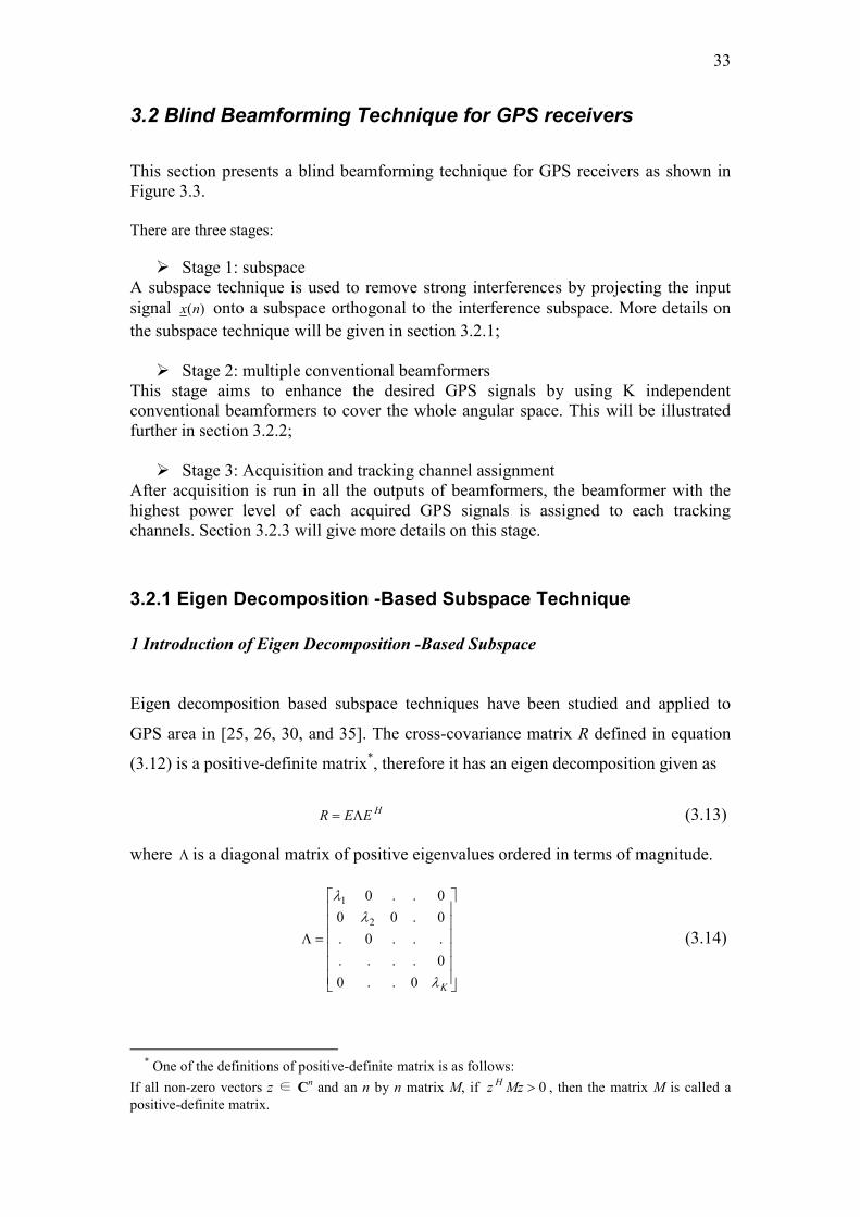
3.2 Blind Beamforming Technique for GPS receivers
This section presents a blind beamforming technique for GPS receivers as shown in
Figure 3.3.
There are three stages:
� Stage 1: subspace A subspace technique is used to remove strong interferences by projecting the input
signal )(nx onto a subspace orthogonal to the interference subspace. More details on
the subspace technique will be given in section 3.2.1;
� Stage 2: multiple conventional beamformers This stage aims to enhance the desired GPS signals by using K independent
conventional beamformers to cover the whole angular space. This will be illustrated
further in section 3.2.2;
� Stage 3: Acquisition and tracking channel assignment After acquisition is run in all the outputs of beamformers, the beamformer with the
highest power level of each acquired GPS signals is assigned to each tracking
channels. Section 3.2.3 will give more details on this stage.
3.2.1 Eigen Decomposition -Based Subspace Technique
1 Introduction of Eigen Decomposition -Based Subspace
Eigen decomposition based subspace techniques have been studied and applied to
GPS area in [25, 26, 30, and 35]. The cross-covariance matrix R defined in equation
(3.12) is a positive-definite matrix*, therefore it has an eigen decomposition given as
HEER Λ= (3.13)
where Λ is a diagonal matrix of positive eigenvalues ordered in terms of magnitude.
=Λ
Kλ
λλ
0..0
0....
...0.
0.00
0..0
2
1
(3.14)
* One of the definitions of positive-definite matrix is as follows:
If all non-zero vectors z ∈ Cn and an n by n matrix M, if 0>Mzz H , then the matrix M is called a
positive-definite matrix.
34
Figure 3.3 Schematic Diagram of Blind Beamforming Technique for GPS Receiver
)(nx
CBF 1
CBF K
Tracking
Channel 1
Acquisition
and
assigning
channels
Subspace
(P)
Tracking
Channel M
Stage 1 Stage 2 Stage 3
35
Kλλλ ,....,, 21 are eigenvalues and Kλλλ ≥≥≥ ....21 >0. The ordered set of eigenvalues
Kλλλ ,....,, 21 is called the eigen spectrum.
The K by K matrix E is the matrix whose columns are the eigenvectors corresponding to
Kλλλ ,....,, 21 respectively.
],...,,[ 21 KeeeE = (3.15)
The eigenvectors Keee ,...,, 21 are orthogonal to one another, i.e., 021=k
H
k ee for any 1k ,
2k =1, 2… K and 21 kk ≠ ; when 21 kk = , 121=k
H
k ee*. Any subset of eigenvectors spans a
subspace which is orthogonal to the subspace spanned by the remaining eigenvectors.
2 Subspaces for the GPS Case
As stated in the signal model in 3.1, in the GPS case, the interferences are dominating
in the overall cross-covariance matrix R (see Equation 3.12). Therefore, after eigen
decomposition of R, when the GPS components in equation (3.12) are ignored, the L
biggest eigenvalues correspond to strong interferences. That is Lλλλ ,....,, 21 and
Leee ,...,, 21 correspond to L uncorrelated interferences, and KLL λλλ ,....,, 21 ++ and the
space spanned by KLL eee ,...,, 21 ++ will only have components of the GPS signals and
components of background noise† in it. Denoting the interference subspace by intS and
GPS plus noise subspace gnS . Then we have
},.....,,{ 21int LeeespanS = (3.16)
},.....,,{ 21 KLLgn eeespanS ++= (3.17)
The interference subspace intS and signal plus noise subspace gnS are orthogonal to
each other. Therefore, when we project the received digitized signal )(nx onto signal
plus noise subspace gnS , the strong interference can be removed. Denoting the
projection matrix of subspace gnS by gnP‡, then we have
∑+
=K
L
H
llgn eeP
1
(3.18)
* By definition eigenvectors have unity magnitude. † This conclusion is made under the assumption that GPS signals and interference are not coincident
in angle. Also notice that all L interferences contribute to each of the eigen values Lλλλ ,....,, 21 and
there is not a one-to-one correspondence. ‡ There is another method to develop this projection matrix. Assuming V is interference subspace and
of full rank, then the projection matrix P of the subspace that is orthogonal to V
is: HH VVVVIP 1)( −−= , where the term HH VVV 1)( − is called Moore-Penrose Pseudo inverse of the
interference subspace V [41].
36
The interference-free output sub
y is
)(nxPy gnsub= (3.19)
3 Estimating the Number of Interferences
It can be seen from equation (3.16) and (3.17) that to apply the above subspace
technique successfully, it is essential to know the number of interferences present in
the received data. We assume that GPS signals are well below the noise and hence
detecting the number of interference is equivalent to detecting the number of signals
incident on the array. When it is difficult to distinguish the number of interferences by
eye from the eigen spectrum, there are some mathematical techniques available to
assist in the decision. There are two criteria that have been shown to be effective. One
is the Akaike Information Criterion (AIC) and the other one is Minimum Description
Length (MDL). Theses two criteria make use of the number of samples used to
estimate the cross-covariance matrix and the number of element antennas [7].
Assume the noise has a normal distribution, the AIC technique calculates a function
AIC (L):
)12(
ˆ)(
1
ˆ
ln)()(
1
)/(1
1 +−+
−
−−=
∑
∏
+=
−
+=LKL
LK
LKNLAICK
Ll
l
LKK
Ll
l
λ
λ
(3.20)
Here, N is the number of samples used to estimate the cross-covariance matrix, K
again is the number of element antennas and L is the estimated number of
interferences. The lλ̂ are the eigenvalues from estimated cross-covariance matrix R̂ ,
where ^ denotes an estimate of the actual values. The number of interferences L is the
value that minimises AIC(L).
The MDL technique uses a very similar function:
)ln(2
)12(
ˆ)(
1
ˆ
ln)()(
1
)/(1
1N
LKL
LK
LKNLMDLK
Ll
l
LKK
Ll
l
+−+
−
−−=
∑
∏
+=
−
+=
λ
λ
(3.21)
Both AIC and tend to overestimate the number of sources. When used on a simulated
data, both techniques classified the weak GPS signals as noise sources. Therefore,
they were not used and were replaced by a simple threshold algorithm.
37
Ignoring multipath effects, non-GPS signals arriving from different directions are
assumed to be interferences that are uncorrelated to each other and much stronger than
background noise, it is reasonable to regard any signal with a power significantly
bigger than that of the background receiver noise as an interference. Therefore, in the
simulation, a threshold is used to estimate the number of interferences from the eigen
spectrum. The threshold is set to be 5dB above the estimated noise power in order to
take into account the statistical variation of the estimated noise floor. That is, the
number of eigenvalues that are bigger than this threshold is assumed equal to the
number of interferences. This estimate is then used to distinguish the interference
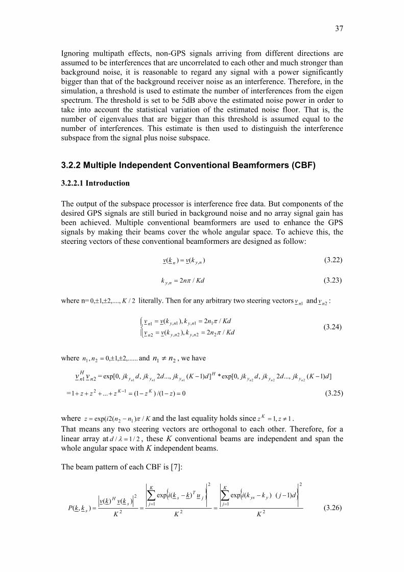
The output of the subspace processor is interference free data. But components of the
desired GPS signals are still buried in background noise and no array signal gain has
been achieved. Multiple conventional beamformers are used to enhance the GPS
signals by making their beams cover the whole angular space. To achieve this, the
steering vectors of these conventional beamformers are designed as follow:
)()( ,nyn kvkv = (3.22)
Kdnk ny /2, π= (3.23)
where n= 2/,....,2,1,0 K±± literally. Then for any arbitrary two steering vectors 1nv and 2nv :
==
==
Kdnkkvv
Kdnkkvv
nynyn
nynyn
/2),(
/2),(
22,2,2
11,1,1
π
π (3.24)
where ,......2,1,0, 21 ±±=nn and 21 nn ≠ , we have
21 n
H
n vv = ])1(...,2,,0exp[*])1(...,2,,0exp[222111
dKjkdjkdjkdKjkdjkdjknnnnnn yyy
Hyyy −−
= 0)1/()1(...1 12 =−−=++++ − zzzzz KK (3.25)
where Knniz /)(2exp( 12 π−= and the last equality holds since 1,1 ≠= zzK .
That means any two steering vectors are orthogonal to each other. Therefore, for a
linear array at 2/1/ =λd , these K conventional beams are independent and span the
whole angular space with K independent beams.
The beam pattern of each CBF is [7]:
{ } { }2
2
1
2
2
1
2
2 )1()(exp)(exp)()(
),(K
djkki
K
ukki
K
kvkvkkP
K
j
yys
K
j
jT
s
sH
s
∑∑==
−−
=
−
== (3.26)
38
The output of each CBF is
)())(()()()( nxkvPnxPkvykvy Hgngn
H
sub
Hcbf === (3.27)
where )(kv is the steering vector of a CBF and )( skv is the steering vector of an incoming
GPS signal. For any incoming GPS signal, the biggest power will be achieved from the output
of a CBF whose steered direction is closest to the DOA of the GPS signal provided there is
not an interference from this direction. The worst case scenario occurs when the DOA of the
GPS signal is located in the middle of two adjacent steered directions. In this case the same
power will be observed at the output of two beamformers.
The worst case GPS signal power can be calculated as follows: suppose a GPS signal comes
in the direction Kdnk ys /)12( 1 π+= which is in the middle of Kdnk y /2 11 π= and
Kdnk y /)1(2 12 π+= as shown in figure 3.4. According to equation (3.26), the normalized
power of this GPS signal is
{ }22
2
/22
2
111
min)2/(sin
11
1
11)1()/2/)12((exp
KKe
e
KK
djKdnKdni
PKi
i
K
j
π
ππ
π
π
=−
−=
−−+
=∑=
(3.28)
For K2/π <<1, KK 2/2/sin ππ ≈ ,
222min
4
)2/(
11
ππ=≈
KKP or -3.9dB (3.29)
Therefore, when there is no interference, for any incoming GPS signal well separated from
interferences, at least (10*log10(K)- 3.9) dB array gain* can be achieved by choosing the CBF
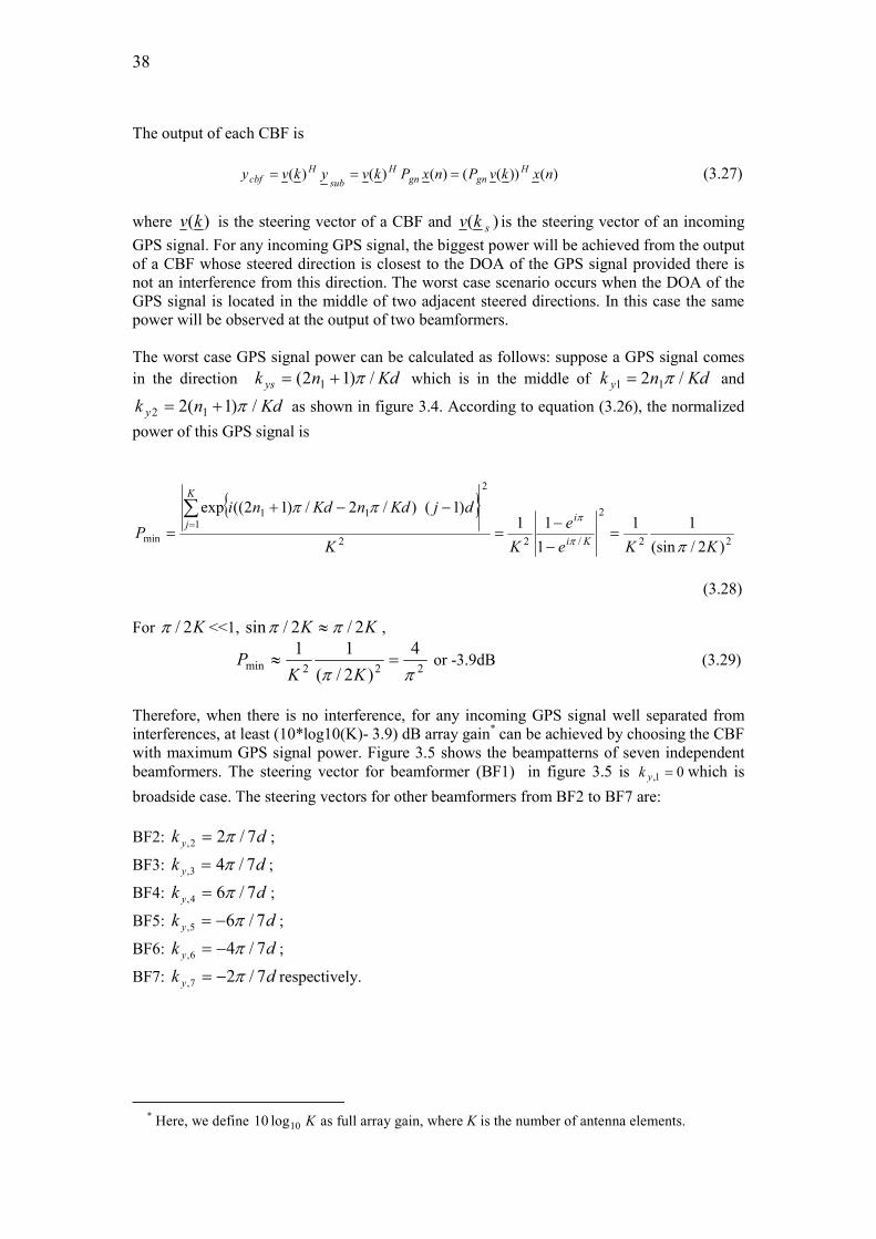
with maximum GPS signal power. Figure 3.5 shows the beampatterns of seven independent
beamformers. The steering vector for beamformer (BF1) in figure 3.5 is 01, =yk which is
broadside case. The steering vectors for other beamformers from BF2 to BF7 are:
BF2: dk y 7/22, π= ;
BF3: dk y 7/43, π= ;
BF4: dk y 7/64, π= ;
BF5: dk y 7/65, π−= ;
BF6: dk y 7/46, π−= ;
BF7: dk y 7/27, π−= respectively.
* Here, we define K10log10 as full array gain, where K is the number of antenna elements.
39
Figure 3.4 GPS Signal Gain in Worst Case Scenario
-1 -0.8 -0.6 -0.4 -0.2 0 0.2 0.4 0.6 0.8 1-90
-80
-70
-60
-50
-40
-30
-20
-10
0
10
unit=pi/d
dB
beampatterns of 7 independent beamformers in wavenumber d/λ=1/2
BF1
BF2
BF3
BF4
BF5
BF6
BF7
BF5 BF6 BF7 BF1 BF2 BF3 BF4
Figure 3.5 Beampatterns of Seven Independent Conventional Beamformers
Kdnk y /2 11 π= Kdnk y /)1(2 12 π+=
0d
-3.9dB
Kdnk ys /)12( 1 π+=
40
3.2.2.2 Overall Beampatterns Combining subspace and multiple independent
beamformers
Throughout the whole thesis, DOAs of GPS and interference are always assumed to
be well separated from each other to make the proposed method work as intended.
However, in this section, the consequences of when the DOAs of GPS and
interferences are close to each other will be discussed to explain why it is so necessary
to have the above assumption.
When the subspace processor and multiple independent beamformers are combined,
the overall beampattern 1_ noverallp steered at 1nv is
2
2
1
2
2
1
2
2
1
1_
)()()()())((
K
kvvP
K
kvvP
K
kvPvP
sH
ngnsH
nHgnsgn
H
n
noverall === (3.30)
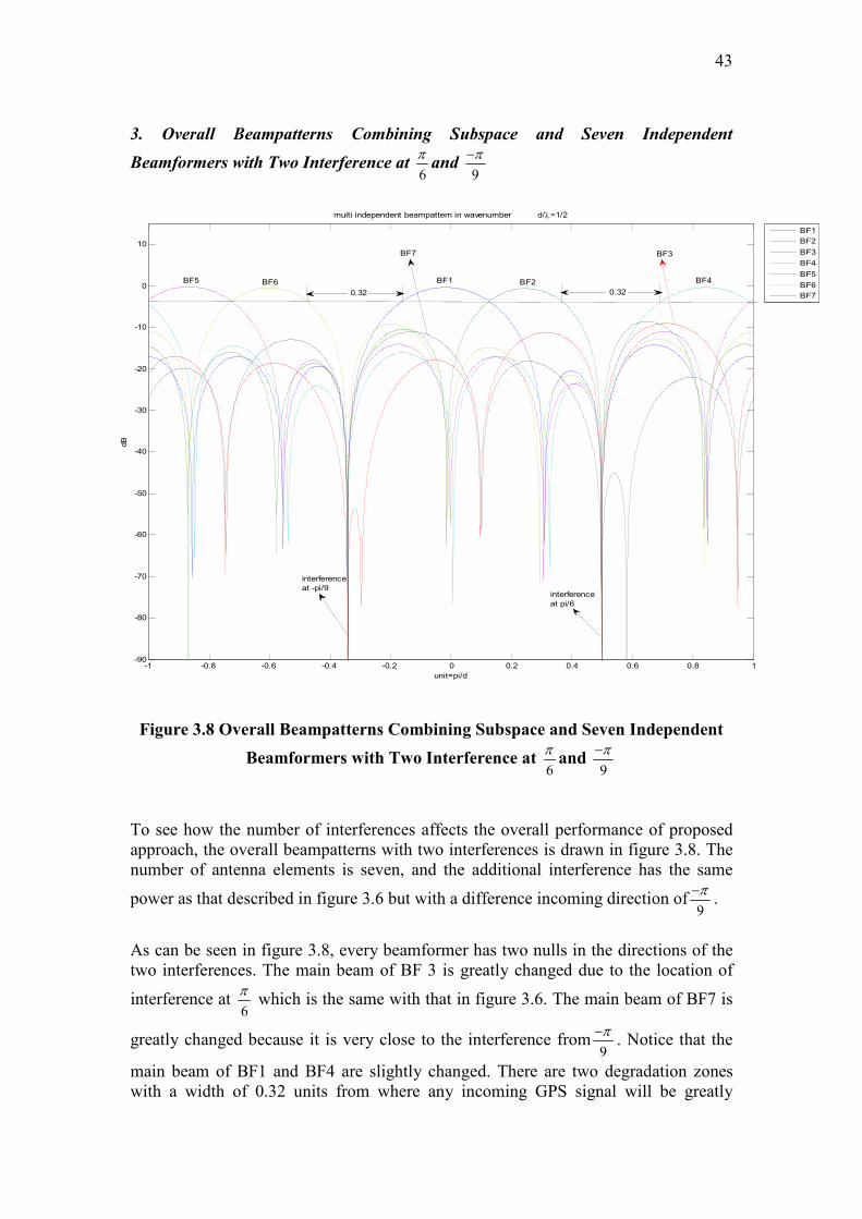
1. Overall Beampatterns Combining Subspace and Seven Independent
Beamformers with Interference at 6
π
-1 -0.8 -0.6 -0.4 -0.2 0 0.2 0.4 0.6 0.8 1-90
-80
-70
-60
-50
-40
-30
-20
-10
0
10
unit=pi/d
dB
overall beampatterns combing subspace and 7 independent beamformers in wavenumber d/λ=1/2
BF1
BF2
BF3
BF4
BF5
BF6
BF7
BF5 BF6 BF7 BF1 BF2 BF4
BF3
-3.9dB0.32
interference at pi/6
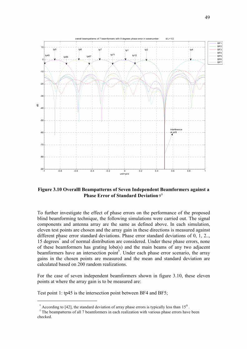
Figure 3.6 Overall Beampatterns Combining Subspace and Seven Independent
Beamformers with Interference at 6
π
41
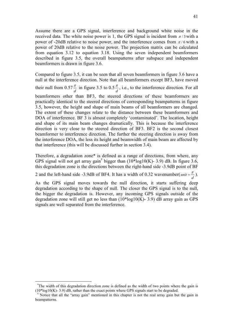
Assume there are a GPS signal, interference and background white noise in the
received data. The white noise power is 1, the GPS signal is incident from 3/π with a
power of -20dB relative to noise power, and the interference comes from 6/π with a
power of 20dB relative to the noise power. The projection matrix can be calculated
from equation 3.12 to equation 3.18. Using the seven independent beamformers
described in figure 3.5, the overall beampatterns after subspace and independent
beamformers is drawn in figure 3.6.
Compared to figure 3.5, it can be seen that all seven beamformers in figure 3.6 have a
null at the interference direction. Note that all beamformers except BF3, have moved
their null from 0.57d
π in figure 3.5 to 0.5
d
π, i.e., to the interference direction. For all
beamformers other than BF3, the steered directions of these beamformers are
practically identical to the steered directions of corresponding beampatterns in figure
3.5, however, the height and shape of main beams of all beamformers are changed.
The extent of these changes relate to the distance between these beamformers and
DOA of interference. BF 3 is almost completely ‘contaminated’. The location, height
and shape of its main beam changes dramatically. This is because the interference
direction is very close to the steered direction of BF3. BF2 is the second closest
beamformer to interference direction. The further the steering direction is away from
the interference DOA, the less its height and beamwidth of main beam are affected by
that interference (this will be discussed further in section 3.4).
Therefore, a degradation zone* is defined as a range of directions, from where, any
GPS signal will not get array gain† bigger than (10*log10(K)- 3.9) dB. In figure 3.6,
this degradation zone is the directions between the right-hand side -3.9dB point of BF
2 and the left-hand side -3.9dB of BF4. It has a width of 0.32 wavenumber(d
unitπ= ).
As the GPS signal moves towards the null direction, it starts suffering deep
degradation according to the shape of null. The closer the GPS signal is to the null,
the bigger the degradation is. However, any incoming GPS signals outside of the
degradation zone will still get no less than (10*log10(K)- 3.9) dB array gain as GPS
signals are well separated from the interference.
*The width of this degradation direction zone is defined as the width of two points where the gain is
(10*log10(K)- 3.9) dB, rather than the exact points where GPS signals start to be degraded.
† Notice that all the “array gain” mentioned in this chapter is not the real array gain but the gain in
beampatterns.
42
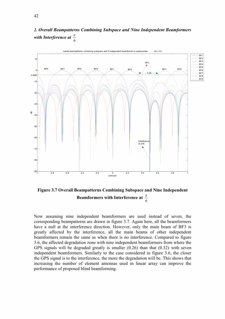
2. Overall Beampatterns Combining Subspace and Nine Independent Beamformers
with Interference at 6
π
-1 -0.8 -0.6 -0.4 -0.2 0 0.2 0.4 0.6 0.8 1-90
-80
-70
-60
-50
-40
-30
-20
-10
0
10
unit=pi/d
dB
overall beampatterns combining subspace and 9 independent beamformer in wavenumber d/λ=1/2
BF1
BF2
BF3
BF4
BF5
BF6
BF7
BF8
BF9
BF6 BF7 BF8 BF9 BF1 BF2 BF4 BF5
BF3
interference
at pi/6
-3.9dB0.26
Figure 3.7 Overall Beampatterns Combining Subspace and Nine Independent
Beamformers with Interference at 6
π
Now assuming nine independent beamformers are used instead of seven, the
corresponding beampatterns are drawn in figure 3.7. Again here, all the beamformers
have a null at the interference direction. However, only the main beam of BF3 is
greatly affected by the interference, all the main beams of other independent
beamformers remain the same as when there is no interference. Compared to figure
3.6, the affected degradation zone with nine independent beamformers from where the
GPS signals will be degraded greatly is smaller (0.26) than that (0.32) with seven
independent beamformers. Similarly to the case considered in figure 3.6, the closer
the GPS signal is to the interference, the more the degradation will be. This shows that
increasing the number of element antennas used in linear array can improve the
performance of proposed blind beamforming.
43
3. Overall Beampatterns Combining Subspace and Seven Independent
Beamformers with Two Interference at 6
πand
9
π−
-1 -0.8 -0.6 -0.4 -0.2 0 0.2 0.4 0.6 0.8 1-90
-80
-70
-60
-50
-40
-30
-20
-10
0
10
unit=pi/d
dB
multi independent beampattern in wavenumber d/λ=1/2
BF1
BF2
BF3
BF4
BF5
BF6
BF7
BF5 BF6 BF1 BF2 BF4
BF3BF7
0.32 0.32
interference
at -pi/9interference
at pi/6
Figure 3.8 Overall Beampatterns Combining Subspace and Seven Independent
Beamformers with Two Interference at 6
πand
9
π−
To see how the number of interferences affects the overall performance of proposed
approach, the overall beampatterns with two interferences is drawn in figure 3.8. The
number of antenna elements is seven, and the additional interference has the same
power as that described in figure 3.6 but with a difference incoming direction of9
π−.
As can be seen in figure 3.8, every beamformer has two nulls in the directions of the
two interferences. The main beam of BF 3 is greatly changed due to the location of
interference at 6
π which is the same with that in figure 3.6. The main beam of BF7 is
greatly changed because it is very close to the interference from9
π−. Notice that the
main beam of BF1 and BF4 are slightly changed. There are two degradation zones
with a width of 0.32 units from where any incoming GPS signal will be greatly
44
degraded. The chance that GPS signals get an array gain of no less than
(10*log10(K)- 3.9) dB is less than the case described in figure 3.6.
4. Summary
When there is no interference present in the received array data, the highest power of
a GPS signal from any direction can always have an array gain of no more than
(10*log10(K)- 3.9) dB; However, when there is one or more interferences existing in
the array data, only GPS signals that are well separated from the interference will
achieve guaranteed array gain of no more than (10*log10(K)- 3.9) dB. Any GPS
signal that is closer to the interference suffers degradation. The closer the GPS signal
is to the interference, the greater the degradation is. In such a situation, the proposed
blind beamforming technique rejects the interference but also degrades the GPS
signal. Thus little or no improvement in C/No is achieved. However, increasing the
number of antenna elements can reduce this negative effect by raising the full array
gain and narrowing the width of degradation zone over which GPS signals have an
array gain of less than (10*log10(K)- 3.9) dB.
Due to the above discussions, GPS signals are always assumed to be well separated
from the interference in this thesis.
3.2.3 Acquisition and Tracking Channel Assignment
This section considers suitable techniques for assigning the beamformer outputs with
the highest C/No of the acquired PRNs to the appropriate receiver channels. Both
acquisition and tracking phases will be considered. The basic operation of the
technique is illustrated in Figure 3.9, where the main channel is always assigned to the
beamformer with the highest C/No.
During signal acquisition, the same Doppler/code phase search algorithm for each SV
can be run in parallel on each beamformer output as the signal direction of arrival is
not known. This will increase the computational load. However, as the C/No is much
higher at the correct beamformer output, shorter integration times can be used for
reliable signal detection, which will again decrease the computational load per
channel.
During signal tracking, the receiver channel needs to switch between different
beamformers as the GPS signal direction of arrival changes. This can be achieved by
monitoring the GPS signal power in the output of the two spatially closest
beamformers. If the power in any of these two beamformers exceeds the power in the
main channel it will be switched to the beamformer with higher power and the two
new spatially closest beamformers will again be monitored. In principle three tracking
loops are required to monitor the GPS signal power at the output of the three selected
beamformers. However, as the Doppler and code phase of the acquired signal on each
of the 3 beamformers are expected to be identical only one complete tracking loop is
required and the remaining channels simply need to de-modulate and integrate the
GPS signal. This means they do not require the loop filters and the early/late
correlators found in standard tracking loops.
45
Figure 3.9 Acquistion and Tracking Assignment
The above structure will be assumed in this thesis, however, there are a number of
alternative ways to connect the tracking loops to the beamformers such as forming a
weighted average of all, or a subset of, the beamformer outputs. Alternatively three
beamformers could be allocated permanently to each tracking channel and be used to
track the GPS signal direction, rather than switching between beamformers. This
would also give the maximum array gain all the time.
When doing acquisition and tracking channel assignment, the acquisition function
from [17] was adjusted to suit the proposed algorithm and the tracking function was
used directly. Appendix A gives the detailed implementation of the proposed
algorithm and Appendix B gives the main MATLAB functions used in the
simulations.
3.3 Projection Matrix P in Subspace
This section shows that the projection matrix P can often be approximated by 1−R ,
which leads to an interesting comparison between this technique and multiple MVDR
beamformers, as well as an alternative way of deriving the P matrix (or 1−R ) based on
the multiple null steering technique.
3.3.1 Projection Matrix P and Inverse of Cross-Covariance Matrix
Recall that in equation (3.13), we have HEER Λ= . For a positive-definite matrix such
as cross-covariance matrix R, the inverse of R can be written as
HEER 11 −− Λ=
H
ii
K
i i
ee∑=
=1
1
λ (3.31)
PRN 11
BF-p1
BF-p
BF-p2
Simplified
Tracking
loop
Simplified
Tracking
loop
Channel m
BF-p3
Time t
BF-p1
BF-p
BF-p2
Simplified
Tracking
Simplified
Tracking
loop
Channel m
BF-p3
Time t’
46
where λ,,ΛE and e are defined in equation (3.14) and (3.15), K is the number of
element antennas. Assuming there are L (L<K) interferences and the variance of noise
plus weak GPS signals is 1( 12 =nσ ), equation (3.31) can be written as
H
ii
K
Li i
H
ii
L
i i
eeeeR ∑∑+==
− +=11
1 11
λλ
H
ii
K
Li
H
ii
L
i i
eeee ∑∑+==
+=11
1
λ
gnH
ii
L
i i
Pee +=∑=1
1
λ (3.32)
where gnP is defined in (3.18).
Comparing equation (3.32) and equation (3.18), we can find:
(1) When there is no interference, gngn PPR =+=− 01 ; IRL =⇒= −10 .
(2) When the interference is very strong, that is iλ >>1 (i=1, 2, L) and iλ1→ 0, the first
part of equation (3.32) approximates zero. Then we have gnPR ≈−1 ;
(3) When the interference is not very strong but still detectable, there is a big
difference between 1−R and projection matrix gnP .
When case (1) or (2) happens, gnP is equal or close to 1−R , this leads to two interesting
findings:
� The combination of subspace and multiple conventional beamforming stage will work like multiple MVDR beamformers;
� An alternative way to implement subspace using multiple null steering arrays.
They will be discussed in the following subsections.
3.3.2 Blind beamforming and Multiple MVDR Beamforming
When combining the subspace projection method with a conventional beam steered in
direction k , the output is given by:
)())(()()()( nxkvPnxPkvykvy Hgngn
H
sub
Hcbf ===
For simplicity, above equation can be rewritten as
)()( nxvPy H= (3.33)
Let vPw = , when PR ≈−1 , we have
vRw 1−= (3.34)
47
Comparing equation (3.34) with equation (2.19), we find the difference between the
weight vector in (3.34) and the weight vector of MVDR beamformer is a
scalarvRv
H 1
1
−. Therefore, the combination of subspace and each conventional
beamformer works like a MVDR beamformer when PR =−1 . The combination of
stage 1 and stage 2 works like multiple MVDR beamformers steered in orthogonal
directions, covering the entire angular space.
3.3.3 An alternative Calculation of Subspace
If we approximate P by 1−R , then P can be calculated from N null steering algorithms
with a different reference channel.
From (3.19), the output of subspace can be rewritten as
)()( 2
1
2
1
nx
w
w
w
nxP
y
y
y
y
H
K
H
H
gn
K
sub
==
=MM (3.35)
=
=
=
⇒
)(
)(
)(
22
11
nxwy
nxwy
nxwy
H
KK
H
H
M (3.36)
and
=
=
=
KgnK
gn
gn
Pw
Pw
Pw
δ
δδ
M
22
11
(3.37)
Where
=
0
0
1
1M
δ ,
=
0
0
1
0
2
M
δ , …
=
1
0
0
M
Kδ
When gnPR ≈−1 , the equation (3.37) can be rewritten as
=
=
=
−
−
−
KRKw
Rw
Rw
δ
δδ
11
21
2
11
1
M (3.38)
48
Comparing equation (3.38) with equation (2.15) we find that, except for the scalar
k
T
kR δδ 1
1
− ( ),2,1 Kk L= each row of the projection matrix contains the weights of a
null steering beamformer. The thk first row of the projection matrix contains the
weights of a null steering beamformer that uses the thk antenna as the reference
antenna. This indicates that when PR =−1 , it is possible to perform the subspace
technique using multiple null steering beamformers.
3.4 Blind Beamforming and Array Phase Error
One of the goals of the proposed blind beamforming algorithm is to achieve an array
gain of more than (10*log10(K)- 3.9) dB for all incoming GPS signals that are well
separated from the interference. However, this conclusion no longer holds in the
presence of phase errors.
3.4.1 Description of Simulations
Assuming a random phase error ke is added to each antenna element*, where k =1,2,..,
K and K is the number of antenna elements in the array. The array phase error ke is
measured in degrees and has a normal distribution with zero mean and a standard
deviation of δ . The weight vector in the presence of phase errors is denoted by 'kW ,
and kk vPW '' = , where kv is the steering vector of beamformer k which is one of the
independent beamformers defined in 3.2.2. 'P is as the projection matrix derived from
the cross covariance matrix 'R , as defined in equations 3.18 &3.12 respectively, but
suitably modified to include array phase errors. To illustrate the effect of phase errors
on the blind beamforming technique, a single example will first be analysed followed
by a more detailed investigation. Assuming there is a strong interference from
6/π with a power of 20dB above the background noise power and a GPS signal from
9
π−with a power of 20dB below the noise. Figure 3.10 shows the beampatterns of
seven independent beamformers with 09 phase error standard deviation. The steered
directions of the seven beamformers are the same as those in figure 3.6. When
comparing with figure 3.6, it can be seen that the shape, general location and the peak
values† of the main lobe of each independent beamformer have slightly changed due
to the phase errors, but the changes to the side lobe structure are the greatest.
However, all beamformers have a deep null in the direction of interference which
means the blind beamforming technique is still able to eliminate interference
effectively even with phase errors.
* In this simulation, the phase error is added to each element of the steering vector.
† The peak value means the array gain in the steered direction of each independent beamformer. When
there is no phase error, this peak value is always 0dB which means of full array gain. However, the
existence of phase error makes it lower than full array gain.
49
-1 -0.8 -0.6 -0.4 -0.2 0 0.2 0.4 0.6 0.8 1-90
-80
-70
-60
-50
-40
-30
-20
-10
0
10
unit=pi/d
dB
overall beampatterns of 7 beamformers with 9 degrees phase error in wavenumber d/λ=1/2
BF1
BF2
BF3
BF4
BF5
BF6
BF7
interference
at pi/6
tp71 tp12
tp2tp7tp5
tp56
tp6
tp67
tp1 tp4
tp45
Figure 3.10 Overalll Beampatterns of Seven Independent Beamformers against a
Phase Error of Standard Deviation 09
To further investigate the effect of phase errors on the performance of the proposed
blind beamforming technique, the following simulations were carried out. The signal
components and antenna array are the same as defined above. In each simulation,
eleven test points are chosen and the array gain in these directions is measured against
different phase error standard deviations. Phase error standard deviations of 0, 1, 2..,
15 degrees* and of normal distribution are considered. Under these phase errors, none
of these beamformers has grating lobe(s) and the main beams of any two adjacent
beamformers have an intersection point†. Under each phase error scenario, the array
gains in the chosen points are measured and the mean and standard deviation are
calculated based on 200 random realizations.
For the case of seven independent beamformers shown in figure 3.10, these eleven
points at where the array gain is to be measured are:
Test point 1: tp45 is the intersection point between BF4 and BF5;
* According to [42], the standard deviation of array phase errors is typically less than 015 .
† The beampatterns of all 7 beamformers in each realization with various phase errors have been
checked.
50
Test point 2: tp5 is the peak value of BF5;
Test point 3: tp56 is the intersection point between BF5 and BF6;
Test point 4: tp6 is the peak value of BF6;
Test point 5: tp67 is the intersection point between BF6 and BF7;
Test point 6: tp7 is the peak value of BF7;
Test point 7: tp71 is the intersection point between BF7 and BF1;
Test point 8: tp1 is the peak value of BF1;
Test point 9: tp12 is the intersection point between BF1 and BF2;
Test point 10: tp2 is the peak value of BF2;
Test point 11: tp4 is the peak value of BF4;
3.4.2 Discussions
Figure 3.11 shows the mean of array gain for all chosen points under various standard
deviations of phase errors. The upper plot is the mean array gain of the peak value
(the peak value direction is the steered direction when there is no phase error) for each
beamformer and the lower plot is the mean array again at the intersection points.
Figure 3.12 shows the standard deviation of the array gain with various phase errors
averaged over 200 realizations.
1. Array Gain without Phase Errors
First consider the impact of an interference on the blind beamforming algorithm in the
absence of phase errors. As discussed in 3.2.2.3, the steered direction of each
beamformer is not affected significantly, but the gain of beamformers close to the
interference is reduced. This can be seen from the plots in figure 3.11. The upper plot
shows that when there is no phase error, none of the steered directions has full array
gain of 0dB. Test point tp6 and tp7, which are the furthest away from interference (see
figure 3.10), have the highest array gain of -0.1dB and -0.11dB respectively; tp5 and
tp1 are next to tp6 and tp7 and have -0.14dB and -0.18dB array gain respectively; tp4
has -0.31dB array gain, which is noticeably smaller than the above points as it is
closer to interference as well; tp2 has the smallest array gain of -0.63dB, this is
because it is the closest steering direction to the interference, except for BF3 which is
completely ‘contaminated’ and not included in the simulations. It is clear that the
further the steered direction is away from the interference, the less it will be affected
by the interference and the more possible for GPS signals from this direction to
achieve high array gain.
As the existence of a steered null changes the shape of the main beam of the
individual beamformers, the array gain of the intersection points is also changed. Test
point tp 45 has -3.92dB array gain which is similar to when there is no interference.
However, the other intersection points have better array gain than the specified -
3.9dB, especially test point tp12, which is the closest intersection point to the null that
can still be considered well separated from the null.
Therefore, when there are no phase errors and the desired GPS signals are well
separated from the interference, blind beamforming works as intended in terms of
maintaining more than -3.9dB array gain relative to the full array gain. However, the
existence of an interference slightly reduces the array gain for GPS signals even when
they are well separated from the interference.
51
0 5 10 15-0.9
-0.8
-0.7
-0.6
-0.5
-0.4
-0.3
-0.2
-0.1
0
phase error /degree
mean o
f array g
ain
/dB
mean of array gain for steered directions with phase errors, 200 realizations,7 antennas
tp5
tp6
tp7
tp1
tp2
tp4
0 5 10 15-4.2
-4.1
-4
-3.9
-3.8
-3.7
-3.6
-3.5
-3.4
-3.3
-3.2
phase error /degree
mean o
f array g
ain
/dB
mean of array gain for intersection points with phase errors, 200 realizations,7 antennas
tp56
tp67
tp71
tp12
tp45
Figure 3.11 Mean of Array Gain against Standard Deviation of the Phase Error
for 7 Antennas
52
0 5 10 150
0.05
0.1
0.15
0.2
0.25
0.3
0.35
phase error /degree
standard deviation of array gain/dB
std deviation against phase errors over 200 realizations with a strong interference,7 antennas
tp4
tp45
tp5
tp56
tp6
tp67
tp7
tp71
tp1
tp12
tp2
Figure 3.12 Standard Deviation of Array Gain against Standard Deviation of the
Phase Error for 7 Antennas
2. Array Gain with Phase Errors
Phase errors will degrade the performance of the blind beamforming technique. For
all the peak value directions considered in figure 3.11, the mean array gain decreases
as the phase error increases as can be seen one the upper plot in figure 3.11. As the
phase error standard deviation increases from 00 to 015 , the mean array gain in the
peak value direction is reduced by about 2.1dB. For the intersection point directions,
the mean array gain also decreases as the phase error increases. However, those
directions that have higher array gain in the absence of phase errors degrade more
rapidly when phase errors are introduced. For example, when the phase error
increases from 00 to 015 , the intersection point directions with a bigger initial array
gain such as tp12, tp71 and tp67 are reduced by 0.34dB, 0.38dB and 0.4dB
respectively, while the mean of the array gain for directions with a smaller initial
value such as tp56 and tp45 only decrease by 0.17dB and 0.19dB respectively.
53
The standard deviation of the array gain over 200 realizations for all chosen points is
shown in figure 3.12. The solid lines represent the peak value directions and the
dashed lines represent the intersection point directions. Generally, the deviation for
the peak value directions is smaller than the intersection point directions except tp 2,
which is the closest point to the null among all chosen points and has the steepest
rising curve with phase error. The intersection points tp71, tp12 and tp67 which have
bigger initial mean of array gain than intersection points tp56 and tp45 also have
bigger standard deviation as the phase error increases. The standard deviation of all
points remains within 0.35dB as phase error increases from 00 to 015 .
In summary, the existence of phase error deteriorates the performance of blind
beamforming. It lowers the mean of array gain for all signal directions that are well
separated from the interference. In the worst case scenario, the specified array gain
which is (10*log10(K)- 3.9) dB is not guaranteed anymore. In some situations, the array gain for the worst case scenario is bigger than (10*log10(K)- 3.9) dB while in other situations it is
not. The directions that are closer to the interference tend to be more sensitive to phase errors.
3.5 Summary
This chapter describes a blind beamforming technique which requires no priori
information of received data. It starts from a signal model of this technique, then
moves to a detailed 3-stage structure, including subspace, multiple beamformer and
acquisition and tracking channel assigning; following that, some discussion regarding
the projection matrix in the subspace stage is made; lastly, the effect of interference
and phase errors on the proposed technique are investigated, and it is shown that the
existence of interference and phase errors degrades the performance of the blind
beamforming technique.
54
Chapter 4
Analysis and Comparison of Null Steering, MMSE and the Blind Beamforming technique
It was proposed in chapter 3 that the blind beamforming technique is able to enhance
of GPS signals. In this chapter, the introduced blind beamforming technique is
compared to other widely used techniques—Null Steering and MMSE. The
comparisons are conducted under the following scenarios: simulated input data
without interferences, simulated input data with various strength interferences,
including extreme situations. Details on how to simulate and the programming can be
found in Appendix A.
4.1 No Interference
The results presented in this section are from the simulations with no interference but
one GPS signal in the simulated input data. The GPS signal is from 3
π− and the input
Carrier-to-Noise ratio (C/No) is set to be around 46dB* (after correlation processing).
Different numbers of antennas will be used for the linear array. For each kind of linear
array, the data will be processed using null steering, MMSE and proposed blind
beamforming techniques.
4.1.1 Results
Notice that the full array gain defined in all simulations is 10*log10(K) dB. Figure 4.1
shows the achieved array gain† from three different techniques using a linear array
with 7 antennas. Figure 4.2 and 4.3 show the results from a linear array with 5 and 3
antennas respectively.
* (1)The background Gaussian noise is simulated using command Randn in MATLAB, therefore the
estimated variance of simulated background noise is not always 1. There is a small variation in each
simulated background noise. Thus the calculated C/No is not always the same but it is always around
46dB; (2) in terms of S/N, the input S/N is -14dB.
† Definition of array gain adopted in this thesis is: array gain=
input
beam
NoC
NoC
)/(
)/(, where beamNoC )/(
denotes the Carrier-to-Noise ratio after beamforming and inputNoC )/( denotes the Carrier-to-Noise
ratio before any array processing. Also notice that when there exists an interference, the power of
interference is not considered as a part of this noise.
55
It can be seen from figure 4.1 that when 7 antennas are used, the average array gain
achieved over 10 realizations for null steering, MMSE and blind beamforming is -
1.78dB, 7.53dB and 7.5dB respectively; when the number of antennas are reduced to
5, the average array gain for null steering, MMSE and blind beamforming is -1.2dB,
6.33dB and 6.01dB respectively; for the case with only 3 antennas used, the achieved
array gain for null steering, MMSE and blind beamforming becomes -0.27dB, 4.5dB
and 3.4dB respectively.
It is shown clearly that the MMSE technique is the best among the three techniques
considered and it always achieves the highest array gain. The more antennas that are
used, the more array gain can be achieved from MMSE.
The blind beamforming technique performs better than null steering but worse than
MMSE. When 7 antennas are used, blind beamforming can achieve an array gain as
high as the MMSE technique. When 5 antennas are used, the gap between the array
gain of blind beamforming and MMSE is about 0.3dB. the gap is increased to about
1dB when only 3 antennas are used. Apparently, the number of element antennas
affects the performance of blind beamforming greatly. The more antennas that are
used, the better performance it can achieve.
Negative array gain is obtained for null steering when using a linear array with 7 and
5 antennas. When using 3 antennas only, both negative and positive array gain were
achieved. The performance of null steering using 7 antennas is worse than that using 5
and 3 antennas. Overall, null steering is not able to increase C/No because it pays no
attention to the desired signals as has been stated in 2.2.1.
1 2 3 4 5 6 7 8 9 10
-2
-1
0
1
2
3
4
5
6
7
8
9
repeated simulations
array gain /dB
array gain using a linear array with 7 antennas
full array gain
null steering
MMSE
blind beamforming
Figure 4.1 Array Gain without Interference with 7 Antennas
56
1 2 3 4 5 6 7 8 9 10
-2
-1
0
1
2
3
4
5
6
7
8
9
repeated simulations
array gain /dB
array gain using a linear array with 5 antennas
full array gain
null steering
MMSE
blind beamforming
Figure 4.2 Array Gain without Interference with 5 Antennas
1 2 3 4 5 6 7 8 9 10
-2
-1
0
1
2
3
4
5
6
7
8
9
repeated simulations
array gain /dB
array gain using a linear array with 3 antennas
full array gain
null steering
MMSE
blind beamforming
Figure 4.3 Array Gain without Interference with 3 Antennas
57
4.1.2 Negative Array Gain for Null Steering
An interesting result from above simulations is that negative array gain is achieved
from null steering when there is no interference. As the GPS signal is much weaker
than background noise and it is expected that the estimated cross-covariance matrix is
close to identity matrix. However, the simulations show that this approximation is not
always accurate.
In the above simulations, the input C/No was set to be about 46dB corresponding to a
reasonably weak signal in practice. However, the null steering in MATLAB is able to
detect this weak GPS signal and regards it as interference.
From equation 3.12, when there is no interference and only 1 GPS signal present in
the received data, the cross-covariance matrix can be written as
Hnng vvaIRRR
22 +=+= σ (4.1)
Where gR and nR are cross-covariance matrix of GPS and noise respectively, 2nσ is the
variance of noise, and 2a is GPS signal power, I is the identity matrix, and v is the
steering vector of GPS signal. Assuming the noise power is 1, according to Sherman-
Morrison-Woodbury formula [43], the inverse of cross-covariance matrix can be
written as
vRva
RvvaRRR
nH
nH
nn 12
12111
1 −
−−−−
+−=
2
2
1 Ka
vvaI
H
+−= (4.2)
where K is the number of antennas used in linear array.
Substituting (4.2) into (2.15) we can get the optimum weight vector for null steering
given the fixed SNR.
Given the input C/No= 46dB, the beampatterns of null steering for different number
of antennas is drawn in figure 4.4. It can be seen that a null is put in the direction of
GPS signal which is at 060− . The more antennas that are used, the deeper the null is.
When there are only 3 antennas, the null is almost unnoticeable. The depth of null
varies depending on the number of antennas.
Furthermore, to see how the number of element antennas affects the depth of the null,
other simulations are conducted, the results of which are shown in Figure 4.5 and 4.6.
58
-100 -50 0 50 100-35
-30
-25
-20
-15
-10
-5
degrees
dB
beampattern,d/λ=1/2
20 element
15 element
10 element
7 element
5 element
3 element
Figure 4.4 Beampatterns of Null Steering without interference
3 5 7 10 15 20 30 400
1
2
3
4
5
6
7
8
9
number of antennas
depth of null in null steering /dB
loss of GPS VS number of antennas at C/No=25dB
Figure 4.5 Loss of GPS Power vs. Number of Antennas in Null Steering
Algorithm with a C/No=46dB
59
3 5 7 10 15 20 30 400
5
10
15
20
25
number of antennas
depth of null in null steering /dB
Loss of GPS VS number of antennas at C/No=33dB
Figure 4.6 Loss of GPS Power vs. Number of Antennas in Null Steering
Algorithm with a C/No =49.5dB
Figure 4.5 and 4.6 show the exact attenuation in the GPS direction when there is no
interference. Figure 4.5 is with a C/No =46dB and figure 4.6 is with a C/No=49.5dB.
It can be seen from both figure 4.5 and 4.6 that, the more antennas are used, the more
the GPS signal is attenuated. With the same number of antennas, the stronger the GPS
signal is, the more likely to be regarded as a interference and are more attenuated by
the null steering technique.
4.2 AG vs. Power Level of Interference
In this section, the achieved array gain from the three techniques is tested in an
environment with interferences of various power levels.
4.2.1 One Interference, One GPS Signal
In this simulation, there is only one interference and one GPS signal present in the
input data. GPS signal is from 3
π− with a C/No of 46dB and interference is from
4
π.
The input power of interference is 0dB, 6.02 dB, 13.97dB, 20dB, 26.02dB, 32.04dB,
38.06dB and 40dB respectively. Figure 4.7 shows the simulation results using 7
antennas and figure 4.8 shows the simulation results with only 3 antennas.
When using 7 antennas, the average array gain from null steering, MMSE and blind
beamforming is -2.25dB, 7.36dB and 7.3dB respectively; when only using 3 antennas,
the achieved array gain is 1.12dB, 3.53dB and 3.07dB from null steering, MMSE and
blind beamforming respectively.
60
It can be seen that blind beamforming works as well as MMSE in the environment
with various interference strength when 7 antennas are used. However, when only 3
antennas are used, the difference between blind beamforming and MMSE is bigger.
This is similar to the scenario when there is no interference present in the input data.
Comparing the results from figure 4.7 and 4.8, it can be found that, when 7 antennas
are used, the influence of interference on the performance of both MMSE and blind
beamforming is very small (the average array gain from MMSE decreases from
7.53dB without inference to 7.36dB with interference; the average array gain from
blind beamforming decreases from 7.5dB to 7.3dB). However, when the number of
antennas used is reduced to 3, the influence of an interference on the performance of
MMSE and blind beamforming is bigger, as the average array gain from MMSE
decreases from 4.5dB to 3.53dB, and that from blind beamforming decreases from
3.4dB to 3dB. Furthermore, MMSE seems to be more vulnerable to interference than
blind beamforming when fewer antennas are used.
Notice that when the input interference power is 0dB, which is the same as the total
power of background Gaussian noise with zero mean and variance of 1, it will not be
detected in the blind beamforming technique either in 7 antenna or 3 antenna case due
to the relatively high threshold pre-defined in the subspace technique (see 3.2.1).
However, blind beamforming still works as intended due to the weak strength of
interference and the assumption that it is well separated from DOA of GPS signal.
For null steering, using more antennas is not an advantage when there is only one
interference present. As we can see that the average array gain is -2.25dB with 7
antennas which is worse than 1.12dB obtained from the 3 element array. Another
interesting result is that, when using 3 antennas, null steering has a better performance
operating in an environment with higher interference power, because degrees of
freedom are taken up to steer nulls at interference and hence no longer available to
steer a null at the GPS signal.
0 5 10 15 20 25 30 35 40-5
-4
-3
-2
-1
0
1
2
3
4
5
6
7
8
9
10
power level of interference /dB
array gain /dB
array gain using a linear array with 7 antennas
full array gain
null steering
MMSE
blind beamforming
Figure 4.7 Array Gain vs. Power of Single Interference with 7 Antennas
61
0 5 10 15 20 25 30 35 40-3
-2
-1
0
1
2
3
4
5
power level of interference /dB
array gain /dB
array gain using a linear array with 3 antennas
full array gain
null steering
MMSE
blind beamforming
Figure 4.8 Array Gain vs. Power of Interference with 3 Antennas
4.2.2 Two Interferences, One GPS Signal
In this section, the simulated input data includes two interferences and one GPS
signal. The GPS signal is from 3
π− with a C/No of 46dB. Two interferences are from
4
π and
6
π respectively. 7 scenarios are considered in figures 4.9 and 4.10.
Scenario 1: Two interferences with the same power of 0dB. The power is the same as
background noise power and the power is so weak that they can not be
detected in blind beamforming.
Scenario 2: Two interferences with the same power of 6.02dB. The power is slightly
higher than the background noise power; when using 7 antennas, blind
beamforming can correctly estimate the number of interferences, but
when using 3 antennas, only 1 interference is estimated.
Scenario 3: Two interferences with the same power of 13.98dB;
Blind beamforming can successfully estimate the number of interferences
in both the 7 antenna and the 3 antenna case.
Scenario 4: Two interferences with the same power of 32.04dB;
Blind beamforming can successfully estimate the number of interferences
in both the 7 antenna and the 3 antenna case.
Scenario 5: One interference is 0dB, another one is 32.04dB;
Only 1 interference is detected in both the 7 antenna and 3 antenna case.
62
Scenario 6: One interference is 6.02dB, another one is 32.04dB;
Blind beamforming can give the correct estimate of the number of
interferences when using 7 antennas but only 1 interference is detected
when using 3 antennas.
Scenario 7: One interference is 13.98dB, the other one is 32.04dB.
Blind beamforming can successfully estimate the number of interferences
in both the 7 antenna and 3 antenna case.
As can be seen from figure 4.9 that no matter how strong or weak the two
interferences are, the MMSE and blind beamforming still work well when 7 antennas
are used. The power level of any interference does not significantly affect the
performance of both techniques. The average array gain for MMSE over all scenarios
is 7.27dB and that for blind beamforming is 7.15dB, the performance of blind
beamforming is slightly lower than that of the MMSE.
Compared to figure 4.1 and 4.7, the performance of null steering when there are 2
interferences present is the worst. The average array gain from figure 4.9 is -3.27dB.
From these simulations, when only 3 antennas are used, both MMSE and blind
beamforming are very vulnerable to the number and strength of the interferences. As
can be seen in figure 4.10, when the two interference are both very strong, MMSE and
blind beamforming have their worst performance and do not improve the C/No of the
GPS signal. When the overall strength of the interferences is small, such as scenario
1,2 ,5 and 6, both MMSE and blind beamforming achieve reasonable array gain,
which is between 3dB and 4dB and is close to the performance when there is only one
interference.
In figure 4.10, null steering works well only when both interferences have low power,
such as in scenario 1,2 and 5. when the two interferences are stronger, the
performance of null steering technique fluctuates.
1 2 3 4 5 6 7-5
-4
-3
-2
-1
0
1
2
3
4
5
6
7
8
9
10
scenario 1 to 7
array gain /dB
array gain using a linear array with 7 antennas
full array gain
null steering
MMSE
blind beamforming
Figure 4.9 Array Gain vs. Power of Two Interference with 7 Antennas
63
1 2 3 4 5 6 7-3
-2
-1
0
1
2
3
4
5
scenario 1 to 7
array gain /dB
array gain using a linear array with 3 antennas
full array gain
null steering
MMSE
blind beamforming
Figure 4.10 Array Gain vs. Power of Two Interference with 3 Antennas
4.3 Three Interferences, three antennas
In this simulation, the number of interferences is increased to three when using an
array with three antennas. The GPS signal is from 3
π− with a C/No of 46dB. Three
interferences are from 4
π, 6
π and
9
πrespectively. There are 7 scenarios that are
marked as x-axis in figure 4.11.
Scenario 1: All three interferences are 0dB.
When all three interferences are 0dB, they are as weak as the background noise.
Therefore, they can not be detected in the blind beamforming technique. Blind
beamforming underestimates the number of interference and processes the input
data as the case of no interference present.
Scenario 2: All three interferences are 6.02dB;
Each interference is slightly higher than background noise. However, blind
beamforming still underestimates the number of interferences. Only 1 interference
is detected in blind beamforming.
Scenario 3: All three interferences are 13.98dB;
All three interferences are significantly higher than background noise. But blind
beamforming still underestimates the number of interferences. Only 2
interferences are detected in blind beamforming.
Scenario 4: All three interferences are 32.04dB;
64
In this scenario, all three interference are very strong. Blind beamforming can
successfully estimate the number of interferences.
Scenario 5: Two interferences are 0dB, one interference is 32.04dB;
Only the strong interference is detected in blind beamforming.
Scenario 6: Two interferences are 6.02dB, one interference is 32.04dB;
Two interference are detected in blind beamforming.
Scenario 7: One interference is 6.02dB, two interferences are 32.04dB.
Two interferences are detected in blind beamforming.
1 2 3 4 5 6 7-8
-7
-6
-5
-4
-3
-2
-1
0
1
2
3
4
5
6
scenario 1 to 7
array gain /dB
array gain using a linear array with 3 antennas
full array gain
null steering
MMSE
blind beamforming
Figure 4.11 Array Gain vs. power of three interference using three antennas
When the number of interferences is equal to the number of antennas of an array, if all
three interference are small, or no more than 2 interferences are strong, MMSE still
gives small array gain for the desired GPS signal. The smaller the interference is, the
better performance MMSE can achieve. However, when all three interference are very
strong, MMSE technique can not give any improvement as seen in scenario 4 in figure
4.11, as it can only steer 2 nulls while maintaining a fixed look direction constraint.
When only 3 antennas are used, blind beamforming tends to underestimate the
number of interferences, which makes blind beamforming give reasonable
improvement when the interferences are weak such as scenarios 1, 2 and 5 in figure
4.11. When all interferences are very strong like in scenario 4, blind beamforming
fails to give any improvement like null steering and MMSE. What’s more, blind
beamforming degrades the strength of desired signal more than the other two
techniques. Further simulations show that, if blind beamforming gives the correct
estimate of the number of interference when interference are small, it degrades the
65
desired signal unlike the performance shown in scenario 1,2,3,5,6 and in figure 4.11
where it underestimates the number of interference.
4.4 Summary
This chapter compares null steering, MMSE and blind beamforming in various
interference environments (including an environment without any interference). Some
conclusions can be made as follows from above simulation results:
1. The MMSE is optimal and always gives the best result;
2. Blind beamforming can more reliably achieve performance close to MMSE when more antennas are used such as 7;
3. Blind beamforming is better than null steering in most scenarios;
4. When the number of interferences is close to the number of antennas, the performance of all three techniques degrades. The stronger the interference is,
the more likely it is detected as an interference, and the lower array they can
achieve;
5. The number of antennas has little impact on the performance of null steering when the number of antennas is bigger than the number of interference.
6. Blind beamforming technique introduced in the thesis tends to underestimate the number of interferences especially when the number of antennas is small
such as 3.
66
Chapter 5
Application to Real Data
It has been shown in chapter 4 that, blind beamforming can achieve performance
close to that of MMSE in most scenarios while no prior information is required. In
this chapter, the data from actual GPS antennas from a previous research project is
analysed using blind the beamforming technique to further test its performance on real
data.
5.1 Description of Collection of Data
The collection of the data being analysed was not conducted by the author of the
thesis, but was collected by other University of Adelaide personnel. The remainder of
this section describes the experimental setup and is taken from a description of the
experiment [16].
GPS RF Environment Testbed (GRET) is a 4-channel unit capable of monitoring,
recording and playing back GPS signals in real-time. During the trial, data was
collected from a 4-element antenna array for further post-trial analysis. The antenna
array and supporting hardware were mounted on the rooftop of a van (see Figure 5.1
and 5.2) while GRET was firmly affixed to the van’s interior. Low-loss cables were
used to connect the antenna elements to GRET.
Figure 5.1 Antenna Array and Supporting Hardware (Front View)
CH4 CH3 CH2 CH1
9cm 9cm 9cm Helical
antenna
Metal
plate
67
Figure 5.2 Antenna Array and Supporting Hardware (Side View)
During the recordings, the RF front end down-converts the GPS signals received by
the antennas from the L1 frequency band to an intermediate frequency of 75MHz. The
signals are then amplified by 30dB before they are passed on to the FPGA unit for
further processing. The FPGA unit consists of analogue-to-digital converters (ADCs)
that translate GPS signals into a digital format suitable for storage on standard
computer hard disk drives. The ADCs used a sampling rate of 49.95MHz. Following
the ADCs is a digital filter/mixer giving a final IF frequency of 12.5699MHz.
5.2 Application to Real Data
The blind beamforming technique was shown to perform adequately with simulated
data in chapter 4. In this section, it will be further assessed in a practical environment
by analysing datasets captured from actual GPS antennas. Two data sets are analysed:
the first data set contains no interference/jamming signals while the second set of data
includes a single CW jammer.
5.2.1 Dataset without Interference
This dataset was collected while there was no interference. Firstly, the data from each
antenna channel was processed to acquire the SVs in it and their individual power
level, then all the data from the array was processed using null steering and blind
beamforming respectively. The results are shown in table 5.1.
Due to various practical issues, the original data was not equalized in phase and
amplitude. Therefore an amplitude equalizer is applied before further processing to
make sure the gain from each antenna is equalized.
Metal
plate
Helical
antenna
Low-loss
cable
Connectors
68
Acquired
SV
in
channel 1
(dB)
in
channel 2
(dB)
in
channel 3
(dB)
in
channel 4
(dB)
after null
steering
(dB)
after blind
technique
(dB)
Expected in the
best case scenario
(dB)
Difference between
blind beamforming and
the best case scenario
(dB)
3 29.61 N/A N/A
15 31.37 30.77 31.37 -0.6
16 28.68 30.21 31.54 27.96 33.02 35.07 -2.05
18 30.79 28.37 30.79 -2.42
21 29.51 31.59 29.62 31.34 33.68 -2.34
22 27.88 29.46 33.29 30.51 34.14 35.6 -1.46
26 31.44 30.48 31.44 -0.96
29 28.93 N/A N/A
Table 5.1 Acquired SVs and their C/No in the Data Set without Interference
Array Data from the First 4 channels Array Data from the First 3 channels Acquired
SVs in
Null Steering(dB)
in Blind
Beamforming(dB)
in
Null Steering(dB)
in Blind
Beamforming(dB)
5 33.12 34.50 33.67 36.42
6 33.36 33.28
10 33.60 33.74 33.87 34.07
17 35.01 34.44 34.83
24 33.54
30 34.62 34.74
Table 5.2 Acquired SVs and their C/No in Data Set with an Interference
69
1. SV 16, 21 and 22 are acquired in the data from channel 1 but only SV 16 and 22 are
acquired in channel 2. There is no SV acquired in the data from channel 3. More SVs
are acquired in the data from channel 4 and their strengths are stronger than those in
channel 1 and channel 2. The reason for this is unclear.
2. The null steering algorithm was applied to the antenna array using channel 1 as the
reference. SV 16, 21 and 22 are acquired when using null steering which are the same
satellites as that were acquired in channel 1. The strengths of SV 16 and 21 after null
steering are similar to those in channel 1 but the strength of SV 22 in null steering is
2.63 dB higher than that in channel 1. The strength of SV 16 in channel 2 is 2.25dB
higher than after null steering but the strength of SV 22 is 1.05dB lower than after null
steering. Overall, null steering performs similar or slightly better than using data in
channel 1 but better than using the data in channel 2. However, null steering obtains
noticeably worse performance than using the data in channel 4 directly. In this case,
the choice of reference data is critical for null steering but overall, when there is no
jammer present, null steering provides little improvement as expected.
3. Eight SVs are acquired in the data after blind beamforming. The strength of SV 16
after blind beamforming is 4.34dB and 2.81dB higher than that in channel 1 and
channel 2 respectively. The strength of SV 21 and 22 after blind beamforming is
1.83dB and 6.26dB higher than that in channel 1 respectively. Blind beamforming
provides a consistent improvement over only using the data in channel 1 or channel 2.
For the acquired SVs in both channel 4 and array data after blind beamforming, the
strength of these SVs using blind beamforming is slightly worse than that in channel 4
except for SVs 16 and 22.
Table 5.1 also shows the results that can be achieved in the best* case scenario if a SV
can be acquired in individual channel(s) and blind beamformer. As can be seen the
performance of blind beamforming can never be better than the best case scenario.
The difference between the blind beamforming and the corresponding best case
scenario for the acquired SVs vary from -0.6dB to 2.42dB, which are all within 3.9dB
as expected. One of the causes to the difference is that the GPS signals are not
accurately incident from the steered directions of four independent beamformers in
stage 2. As indicated in 3.2.2.3, the closer the GPS signal is to the steered direction of
a beamformer in stage 2, the higher the array gain can be achieved using blind
beamforming technique. Thus, the bigger difference for SV 16, 18 and 21 that are -
2.05dB, -2.42dB and -2.34dB respectively implies that these three SVs are incident
from the direction close the intersection of two adjacent independent beamformers.
Similarly, the rest of acquired SVs are incident from the direction close to the steered
direction of an independent beamformer.
* The best case scenario assumes the received GPS signals are in-phase.
70
5.2.2 Dataset with a Jammer
A data set with a single jammer was also analysed. In this data set, the jammer was
strong enough to corrupt all GPS signals. Therefore no SV can be acquired from the
data prior to beamforming. The array data is equalized and Hilbert transformed before
using beamforming. After that, the array data is combined using null steering and
blind beamforming techniques respectively. The output of the array from both
techniques is then sent to an acquisition function to detect the GPS signals and
measure the strength of the detected SVs. Although there were 4 antennas used to
collect the data, the data from the 4th antenna/channel had a big phase/amplitude error
that could not be compensated even in the equalization process. Therefore, two array
data sets were tested using null steering and blind beamforming algorithms. The first
data set consists of the data from all 4 channels, but the second data set only includes
data from the first 3 channels. The acquired SVs and their strengths are shown in table
5.2.
1. Array Data from All Four Channels
As can be seen from table 5.2, four SVs were detected after null steering which are
SV 5,6,10 and 17. However, only three SVs are detected after blind beamforming
namely SV 5, 10 and 30. The strengths of SV 5 and 10 in blind beamforming are
1.38dB and 0.14dB higher than in null steering. But SV 6 and 17 can not be detected
using the blind beamforming technique. From the perspective of the number of
detected SVs, null steering has a better performance, because in practice at least four
SVs are required to obtain a GPS navigation solution.
2. Array Data from the First Three Channels
Five SVs are detected after null steering namely SV 5,6,10,17 and 24. SV 24 was not
detected when using the data from all four channels. The strengths of SV 5,6,10 and
17 are similar to the strengths obtained when using all 4 channels.
Four SVs are detected in blind beamforming which are 5,10,17 and 30. SV 17 was not
detected when using the data from all four channels. The S/N of SV 5 is 2.75dB
higher than after null steering. The S/N of SV 10 and 17 is only 0.2dB and 0.4dB
higher than after null steering. From the perspective of the S/N of acquired SVs, blind
beamforming has a slightly better performance than null steering in this array data.
Notice that the S/N of SV 5 is 3.3dB higher than from all four channels which is a
significant improvement, and it may indicate that the DOA of SV 5 is very close to
one of the steered directions in the blind beamforming technique. However note that
null steering detects 5 SVs while blind beamforming only detects 4.
71
3. Summary
From the analysis of table 5.2, it is clear that the array errors affect both null steering
and blind beamforming algorithms. It seems that blind beamforming is more
vulnerable to array errors than null steering. For the SVs that are detected in both null
steering and blind beamforming, blind beamforming increases their S/N over null
steering which is expected and null steering does little because null steering pays no
attention to desired GPS signals. However, in that case, null steering detects one more
SV than blind beamforming.
5.3 Summary
Due to time limitation and various other practical issues, only datasets without a
jammer and with a single strong CW jammer are analysed. Therefore, we have not
analysed how the blind beamforming algorithm works in scenarios that include
various interference such as different waveforms and strengths.
When there is no interference present, blind beamforming works as expected and
better than null steering. However, when there is a strong CW jammer in the received
data, the result displayed some gain but these were not as great as would be expected
under theoretically ideal conditions. Blind beamforming only achieves a slightly
better performance in terms of S/N but is worse in terms of number of signals
detected. This maybe partly due to the small number of antenna elements and array
phase errors. Blind beamforming technique benefits more from the number of
antennas and more vulnerable to array error than null steering.
72
Chapter 6
Conclusion
6.1 Summary
This thesis has presented a blind beamforming technique that is able to mitigate
interference and enhance the desired weak GPS signals without having any priori
information about the DOAs of the GPS signals.
Initially the GPS signal characteristics and GPS receiver structure were introduced.
The effect of interference on the GPS signal and receiver was also addressed. Then
four array processing algorithms were introduced and analysed for GPS applications.
The advantages and limitations of these four algorithms were presented. Finally, a
blind beamforming algorithm was proposed to combine the advantages and
disadvantages of existing algorithms.
The details of the proposed algorithm were given in chapter 3 including a
mathematical signal model, a three-stage processing algorithm and a realistic
simulation of this algorithm. One of the outcomes of this Master project is the
MATLAB software model of the proposed algorithm based on the software-defined
GNSS receiver in [17].
The blind beamforming algorithm together with null steering and MMSE algorithms
were tested in various simulated interference scenarios in chapter 4. The number of
interferences, the number of antenna elements and the strength of interference were
varied in the simulations. The performance of null steering, MMSE and blind
beamforming algorithms were compared in all scenarios and blind beamforming
algorithm showed potential in the simulated environments.
In chapter 5, the blind beamforming and null steering algorithm were applied to real
data that was collected in previous project [16]. However only two data sets were
analysed: one is the data without any jammer and the other one is data with a strong
CW jammer. The performance of blind beamforming and null steering algorithm in
these two data sets was compared. It was shown that blind beamforming algorithm
will potentially improve the SNR of GPS signals in practical situations, but is more
sensitive to system errors reducing the number of SVs detected.
73
6.2 Limitations
There are some critical factors involved in blind beamforming technique which can
also be seen as limitations of this algorithm.
The first limitation is the estimate of the number of interferences in the subspace
stage. To get the correct estimate is very important for blind beamforming to be able
to mitigate the interferences. Two methods were mentioned to estimate the number of
interferences in 3.2.1. One is AIC or MDL, which tends to over-estimate the number
of interferences; the other one is the threshold method. This method uses a fixed
threshold which should be based on an array calibration result. The threshold method
tends to under-estimate the number of interferences especially when the interference
is not very strong. Both over-estimate and under-estimate should be avoided.
However, since the GPS receiver tolerates a weak interference, the threshold method
performs better in situations with weak interference.
To ensure blind beamforming algorithms work as intended, a proper detection scheme
in the acquisition stage is required. The pre-defined threshold in acquisition is critical
in particular. This pre-defined threshold can also be obtained from an array calibration
process. The intermediate frequency used in the detection and the acquisition search
band are also very important.
The blind beamforming algorithm requires a reasonable number of antenna elements
to achieve a significant performance improvement. If the number of antenna elements
used is small such as three, then the improvement of this algorithm is not noticeable
or even worst than null steering in some scenarios. However, in practice, the number
of antenna elements in use is limited by the cost or hardware issues.
Throughout all the simulations in this thesis, the DOAs of the desired GPS signals are
always assumed to be well separated from the DOAs of interference. The proposed
blind beamforming algorithm is a spatial array processing technique. Therefore, GPS
signals will be attenuated when they are too close to the DOAs of interference.
6.3 Recommendations and Extensions
This thesis has demonstrated that the proposed blind beamforming technique is a
viable algorithm for mitigating interference and enhancing the desired weak GPS
signals. However, the subspace technique used in this algorithm involves lots of
computations. More research needs to done on reducing the computations. A fast
subspace technique in [18] might be helpful.
There were only two data sets that were analysed which is not adequate to test the
performance of proposed blind beamforming algorithm in practical environments and
it is recommended that more real data be analysed.
Appendix A
Implementation of proposed blind beamforming technique in MATLAB
In this section, the MATLAB simulation of the blind beamforming technique
described in 3.2 is presented, including essential explanations of the MATLAB code
and the corresponding simulation results.
1 Input Data Generation
This simulation assumes an ideal RF front end which converts the data from all the
element antennas to an Intermediate Frequency (IF) prior to the analogue-to- digital
converter (ADC). Therefore, the digital input data is generated in the signal
generation part. Because the frequency of C/A codes is 1.023 MHz, for simplicity, the
IF frequency is assumed to be 2.046 MHz and the sampling rate is assumed to be
8.184 MHz.
The simulated complex input data has three components: GPS signal, interference and
Gaussian noise.
1 GPS Signal
The GPS signal has three components: navigation data, C/A code and carrier
frequency (see Figure 2.1). Due to the long period of the navigation data compared
with the C/A code and carrier periods, the generation of a GPS signals in this
simulation doesn’t include the navigation data.
The digital frequency of the GPS carrier (0 Doppler) is: 2.046 MHz/8.184 MHz=0.25.
It is reasonable to assume that the maximum Doppler shift between any receiver on
Earth and satellites is + 5 kHz. In terms of digital frequency, the received GPS carrier
frequency is between (0.25-0.00061) to (0.25+0.00061). The frequency search step of
acquisition is assumed to be 500 Hz. Therefore, to make the received GPS signal
discernable from one another, the difference of the digital frequency between each
received GPS signal should be bigger than 5101.6 −× .
(1) Carrier Frequency Generation
Assume there is a GPS signal in view, its elevation angle is phi, azimuth angle is thita,
received carrier frequency if f, the amplitude is amp, and the number of samples to be
generated is number_of_samples, then generation of the sampled carrier and
wavevector k in Matlab are as follow (see function signal_generation in Appendix E):
where x2 is the data matrix of the interference incident on the antenna array, v2 and
k_int are its corresponding steering vector and wavevector. xInt is the sum of all the
interference data if there are more than one point source interference present in the
received data.
3 Gaussian Noise and Overall Simulated data
The Gaussian noise is simply generated using function randn in Matlab:
x_n=randn(size(xGPS));
The overall simulated data on antenna array x is the sum of GPS, interference and
Gaussian noise data matrix:
x=xGPS+xInt+x_n;
The simulated complex input data x is then processed through sequential stages
described in section 3.2.
Figure (3.7) shows the real part of a simulated data*. In this case, there are two input
GPS signals with input C/No of 38.6dB and they come from 060− and
020− respectively.
There are two strong wideband interferences both with a power of 40dB above noise power.
The incoming direction of interferences are 030 and
045 . The variance of Gaussian noise 2nσ is 1.
* This data is the first row of generated array data x.
78
0 1000 2000 3000 4000 5000 6000 7000 8000 9000-30
-20
-10
0
10
20
30
Figure A2 Real Part of Simulated Received Data at One Antenna
2 Simulation of Subspace Technique
This section explains how the subspace technique is implemented in Matlab.
1. Estimate of Cross-covariance Matrix
The subspace method is based on eigen-decomposition of cross-covariance matrix of
the received data x. Since we don’t know the exact cross-covariance matrix of the
received data in practice (but it is known in this simulation), an estimate of this matrix
is calculated through function estimate_R. Under the assumption that received data is
stationary and ergodic, estimate_R works as follow:
function [R]=estimate_R(x) [number_of_antennas,number_of_samples]=size(x); R=[]; for row=1:number_of_antennas for column=1:number_of_antennas R(row,column)=(x(row,:)*x(column,:)')/number_of_samples; end end
2. Estimate the Number of Interferences
The number of strong interferences is estimated from the eigen-spectrum of this
estimated cross-covariance matrix R through function estimate_number_of_int. This
function works as follows: first the built-in command lamda=svd(R) is used to
achieve all eigen-values of R in decreasing order, then assume the smallest eigen
value is the background noise power which is lamda(K) where K is the number of
antennas, next the noise floor is defined in term of dB/Hz as
noiseFloor=10*log10(lamda(K)/fs)+30 in Matlab, last the threshold of detecting the
interference is set to be 5dB above this noise floor which is
threshold=10*log10(K)+5+noiseFloor. The number of eigen value(s) that is/are
bigger than the threshold is regarded as the number of interferences:
79
number_of_int=0; for index=1:K if lamda(index)>threshold number_of_int=number_of_int+1; end end
The final result number_of_int is then passed to subspace function to partition the
interference subspace from overall space.
3. Subspace
The subspace technique is implemented in function subspace. The inputs of this
function are the estimated cross-covariance matrix R, input data x and estimated
number of interferences number_of_int. The outputs of this function include
interference-free subspace_output, the projectionMatrix and noise_subspace that is
orthogonal to interference subspace. Fuction subspace works as follows:
Firstly, the diagonal matrix that contains the eigen values and the matrix whose
columns are eigen vectors are generated through [E,D,E1]=svd(R), where here D is
the matrix defined in Equation 3.14, and E and E1 are the same matrix which is
defined in Equation 3.15. The biggest number_of_int eigen values are corresponding
to interferences, therefore the remaining (K- number_of_int) eigen values are
corresponding to weak GPS signals and Gaussian noise. The eigen vectors
corresponding to (K- number_of_int) smallest eigen values consist of the GPS plus
noise subspace which is orthogonal to interference subspace. GPS_noise_subspace=E(:,number_of_int+1:K)
The projection matrix of this orthogonal matrix is implemented as follows according
to Equation (3.18):
projection_noise=0; for index2=number_of_int+1:K projection_noise=projection_noise+E(:,index2)*E(:,index2)'; end
Finally, the interference-free output subspace_output of the subspace is obtained by
projecting the received data x onto the subspace GPS_noise_subspace:
subspace_output=projection_noise*x
subspace_output then goes through in the following Independent Beamformers stage.
Each column of the projection works as a weight vector from where a beampattern
can be drawn. Figure 3.8 shows the beampatterns of subspace using a linear array
with 7 antennas. It can be seen that two deep nulls are put in the directions of
interferences, which can be successfully mitigated.
80
-100 -80 -60 -40 -20 0 20 40 60 80 100-90
-80
-70
-60
-50
-40
-30
-20
-10
degrees
dB
beampattern,d/λ=1/2
Figure A3 Beampatterns of Subspaces
3 Simulation of Independent Beamforming Technique
This process is implemented in function multi_independent_BF. The inputs of this
function are array data (output of subspace stage) and array position matrix. The
outputs of this functions include the output, steering vector and beampattern of each
individual beamformer ( there are K independent beamformers totally).
The whole function is a big for loop (see Appendix B). Firstly, the wavevectors of each beamformer is defined according to equation (3.31).
There will be K beamformers from 090− to 090 in actual angle. The beamformer with
zero azimuth angle is labelled number 1. The beamformers with positive azimuth
angle from zero are labelled number 2, 3,..till 090 is reached and then the numbering
continues from the beamformer whose steering angle is close to 090− . Eventually, the
beamformer with negative steering angle and just beside beamformer number 1 will
be labelled number K. Figure B4 shows the beampatterns of 7 independent
conventional beamformers and their numbering. The x axis is in unit of
wavenumber/wavevector. The direction information of received data simulated is also
shown in the figure. Table 3.1 shows the corresponding spatial angle of wavenumbers.
81
-1 -0.8 -0.6 -0.4 -0.2 0 0.2 0.4 0.6 0.8 1-80
-70
-60
-50
-40
-30
-20
-10
0
10
20
unit=pi/d
dB
multi independent beampattern in wavenumber d/λ=1/2
CBF5 CBF6 CBF7 CBF1 CBF2 CBF3 CBF4
PRN11 PRN12 interference1interference2
Figure A4 Beampatterns of Independent Conventional Beamformers
Table A1 Corresponding Spatial Angles of Wavenumbers
82
Appendix B
MATLAB Functions
This appendix presents some critical MATLAB functions used in the simulations
1. Main Test Function
2 Signal Generation Function
function [s,k]=signal_generation(f,amp,thita,phi,number_of_samples) %this function generates the simulated incoming GPS signal %inputs: 1)digital frequency % 2)amplitude of the GPS signal % 3)azimuth and elevation angles % 4)the number of samples %outputs: 1)time domain signal % 2)simplified wavevector of the GPS signal N=[0:1:(number_of_samples-1)]; %N=[1:1:number_of_samples]; s=amp*exp(i*2*pi*f*N); %generate complex signal k=pi*[cos(thita)*sin(phi); sin(thita)*sin(phi); cos(phi)]; %generate wave vector k, here we assume that d/lamda=1/2
3 CAcode Generation Function
This function is from [17].
function CAcode = generateCAcode(PRN) % generateCAcode.m generates one of the 32 GPS satellite C/A codes. % % CAcode = generateCAcode(PRN) % % Inputs: % PRN - PRN number of the sequence. % % Outputs: % CAcode - a vector containing the desired C/A code sequence % (chips). %-------------------------------------------------------------------------- % SoftGNSS v3.0 % % Copyright (C) Darius Plausinaitis % Written by Darius Plausinaitis % Based on Dennis M. Akos, Peter Rinder and Nicolaj Bertelsen %-------------------------------------------------------------------------- %This program is free software; you can redistribute it and/or %modify it under the terms of the GNU General Public License %as published by the Free Software Foundation; either version 2 %of the License, or (at your option) any later version. %
83
%This program is distributed in the hope that it will be useful, %but WITHOUT ANY WARRANTY; without even the implied warranty of %MERCHANTABILITY or FITNESS FOR A PARTICULAR PURPOSE. See the %GNU General Public License for more details. % %You should have received a copy of the GNU General Public License %along with this program; if not, write to the Free Software %Foundation, Inc., 51 Franklin Street, Fifth Floor, Boston, MA 02110-1301, %USA. %-------------------------------------------------------------------------- %CVS record: %$Id: generateCAcode.m,v 1.1.2.5 2006/08/14 11:38:22 dpl Exp $ %--- Make the code shift array. The shift depends on the PRN number ------- % The g2s vector holds the appropriate shift of the g2 code to generate % the C/A code (ex. for SV#19 - use a G2 shift of g2s(19) = 471) g2s = [ 5, 6, 7, 8, 17, 18, 139, 140, 141, 251, ... 252, 254, 255, 256, 257, 258, 469, 470, 471, 472, ... 473, 474, 509, 512, 513, 514, 515, 516, 859, 860, ... 861, 862 ... end of shifts for GPS satellites ... Shifts for the ground GPS transmitter are not included ... Shifts for EGNOS and WAAS satellites (true_PRN = PRN + 87) 145, 175, 52, 21, 237, 235, 886, 657, ... 634, 762, 355, 1012, 176, 603, 130, 359, 595, 68, ... 386]; %--- Pick right shift for the given PRN number ---------------------------- g2shift = g2s(PRN); %--- Generate G1 code ----------------------------------------------------- %--- Initialize g1 output to speed up the function --- g1 = zeros(1, 1023); %--- Load shift register --- reg = -1*ones(1, 10); %--- Generate all G1 signal chips based on the G1 feedback polynomial ----- for i=1:1023 g1(i) = reg(10); saveBit = reg(3)*reg(10); reg(2:10) = reg(1:9); reg(1) = saveBit; end %--- Generate G2 code ----------------------------------------------------- %--- Initialize g2 output to speed up the function --- g2 = zeros(1, 1023); %--- Load shift register --- reg = -1*ones(1, 10);
84
%--- Generate all G2 signal chips based on the G2 feedback polynomial ----- for i=1:1023 g2(i) = reg(10); saveBit = reg(2)*reg(3)*reg(6)*reg(8)*reg(9)*reg(10); reg(2:10) = reg(1:9); reg(1) = saveBit; end %--- Shift G2 code -------------------------------------------------------- %The idea: g2 = concatenate[ g2_right_part, g2_left_part ]; g2 = [g2(1023-g2shift+1 : 1023), g2(1 : 1023-g2shift)]; %--- Form single sample C/A code by multiplying G1 and G2 ----------------- CAcode = -(g1 .* g2);
4 Spatial Filter
function [x,v]=spacial_filter(s,k,u) %This function performs spatial filter %assume: 1)K antennas are equal-spaced along y axis % 2)the spacing is half of the freqency length,that is d/lambda=1/2. %inputs: % 1)time domain GPS signal s % 2)wavevector k of the GPS signal % 3)coordinates of array antennas x=[]; % antennas output vector v=[]; % steering vector for each signal for index=1:size(u,2) v(index)=exp(i*k'*u(:,index)); %build steering vector x(index,:)=s*v(index); %generate antenna output end v=v.'; %transpose steering vector to make it column vector
5 Estimate the Cross-Covariance Matrix
function [R]=estimate_R(x) %estimate covariance matrix R of input x [number_of_antennas,number_of_samples]=size(x); R=[]; for row=1:number_of_antennas for column=1:number_of_antennas R(row,column)=(x(row,:)*x(column,:)')/number_of_samples; end end
6 Estimate the Number of Interference
function [number_of_int]=estimate_number_of_int(R,K,fs)
85
%this function performs the estimate of number of interferences %assumptions:the back ground noise power is 1 %inputs: 1)cross-covariance matrix % 2)the number of antennas % 3)the number of samples %output: the estimate of interference lamda=svd(R); lamda=10*log10(lamda); number_of_int=0; for index=1:K if lamda(index)>5 %in practical GPS case,the interference power is always assumed to be 5dB %higher than gausian noise floor. number_of_int=number_of_int+1; end end
7 Implementation of Subspace
function [subspace_output,projection_of_orthogonal_int_sub,GPS_noise_subspace]=subspace(R,x,number_of_int) %this is subspace function for the case that there are N uncorrelated %interferences and noise. %the purpose of this function is to reject interference and yield receiver %outputs where there is no interference. [E,D,E1]=svd(R); %eigen decomposition.D is K*K diagonal matrix whose diagonal are eigen %values and the columns of E is the corresponding eigen vectors %rearrange the order of E to make sure that the first N eigen vectors %correspond the first N biggest eigen values %re-arrange the eigen vector matrix for index=1:length(R) diaEle(index)=D(index,index); end [valueOfEigen,positionOfEigen]=sort(diaEle,2,'descend'); for index=1:length(R) EE(:,index)=E(:,positionOfEigen(index)); end E=EE; K=size(R,1); GPS_noise_subspace=E(:,number_of_int+1:K);
86
%find noise subspace which is spined by the eigen vectors corresponding to %smallest eigen values int_sub=E(:,1:number_of_int); %find interference subspace which is spined by the eigen vectors corresponding to %largest eigen values MPPI_of_int_sub=inv(int_sub'*int_sub)*int_sub'; %pseudo-inverse of matrix projection_of_orthogonal_int_sub=eye(K)-int_sub*MPPI_of_int_sub; %projection matrix of the orthogonal subspace subspace_output=projection_of_orthogonal_int_sub*x; %output of subspace stage
8 Implementation of Multiple Conventional Beamformers
function [y,vy,outputPower]=multi_independent_BF(x,u) %this function is to form K independent beamformers to cover the whole angular space %we assume receivers are equi-spaced along y axis %inputs: 1)u--the array position matrix U(the column of U is the position of % each antenna).U is a 3 by K matrix % 2)input data %outputs: 1)output of K independent beamformers that cover the whole angular space % 2)vy--the steering vector matrix vy.vy is a k by k matrix,whose % columns are the steering vectors that are orthogonal to each % other % 3)the power of each beamformer output K=size(u,2); %calculating the number of receivers from postion matrix for index1=1:K % generate K orthogonal steering vectors/wavenumbers if (index1-1)<=(K-1)/2 ky(index1)=(2*pi/K)*(index1-1); else ky(index1)=-(2*pi/K)*(K-index1+1); end %if we only generate K independent BF,then they only cover half of angular %space actually.Because of the symmetry of linear array,when index1 take %values from 1 to K,only [0,pi] space will be covered. for index2=1:K
87
vy(index2,index1)=exp(i*(ky(index1)*u(2,index2))); end y(index1,:)=(1/K)*vy(:,index1)'*x; %y is a matrix with the same size as x p=mean((abs(y(index1,:))).^2); p=10*log10(p); outputPower(index1)=p; end
9 Acquistion
This function is based on the function in [17].
function acqResults = acquisition(s, settings) %Function performs cold start acquisition on the collected "data". It %searches for GPS signals of all satellites, which are listed in field %"acqSatelliteList" in the settings structure. Function saves code phase %and frequency of the detected signals in the "acqResults" structure. % %acqResults = acquisition(s, settings) % % Inputs: % s - 11 ms of raw signal from the front-end % settings - Receiver settings. Provides information about % sampling and intermediate frequencies and other % parameters including the list of the satellites to % be acquired. % Outputs: % acqResults - Function saves code phases and frequencies of the % detected signals in the "acqResults" structure. The % field "carrFreq" is set to 0 if the signal is not % detected for the given PRN number. %-------------------------------------------------------------------------- % SoftGNSS v3.0 % % Copyright (C) Darius Plausinaitis and Dennis M. Akos % Written by Darius Plausinaitis and Dennis M. Akos % Based on Peter Rinder and Nicolaj Bertelsen %-------------------------------------------------------------------------- %This program is free software; you can redistribute it and/or %modify it under the terms of the GNU General Public License %as published by the Free Software Foundation; either version 2 %of the License, or (at your option) any later version. % %This program is distributed in the hope that it will be useful, %but WITHOUT ANY WARRANTY; without even the implied warranty of
88
%MERCHANTABILITY or FITNESS FOR A PARTICULAR PURPOSE. See the %GNU General Public License for more details. % %You should have received a copy of the GNU General Public License %along with this program; if not, write to the Free Software %Foundation, Inc., 51 Franklin Street, Fifth Floor, Boston, MA 02110-1301, %USA. %-------------------------------------------------------------------------- %CVS record: %$Id: acquisition.m,v 1.1.2.12 2006/08/14 12:08:03 dpl Exp $ %% Initialization ========================================================= % Find number of samples per spreading code samplesPerCode = round(settings.samplingFreq / ... (settings.codeFreqBasis / settings.codeLength)); % Create two 1msec vectors of data to correlate with and one with zero DC signal1 = s(1 : samplesPerCode); signal2 = s(samplesPerCode+1 : 2*samplesPerCode); signal3=[signal1,signal2]; variance1=var(signal1); variance2=var(signal2); signal0DC = s - mean(s); % Find sampling period ts = 1 / settings.samplingFreq; % Find phase points of the local carrier wave phasePoints = (0 : (samplesPerCode-1)) * 2 * pi * ts; % Number of the frequency bins for the given acquisition band (500Hz steps) numberOfFrqBins = round(settings.acqSearchBand * 2) + 1; % Generate all C/A codes and sample them according to the sampling freq. caCodesTable = makeCaTable(settings); %--- Initialize arrays to speed up the code ------------------------------- % Search results of all frequency bins and code shifts (for one satellite) results = zeros(numberOfFrqBins, samplesPerCode); % Carrier frequencies of the frequency bins frqBins = zeros(1, numberOfFrqBins);
89
%--- Initialize acqResults ------------------------------------------------ % Carrier frequencies of detected signals acqResults.carrFreq = zeros(1, 32); % C/A code phases of detected signals acqResults.codePhase = zeros(1, 32); % Correlation peak ratios of the detected signals acqResults.peakMetric = zeros(1, 32); acqResults.peakMetric1 = zeros(1, 32); acqResults.peakMetric2 = zeros(1, 32); fprintf('('); % Perform search for all listed PRN numbers ... for PRN = settings.acqSatelliteList %% Correlate signals ====================================================== %--- Perform DFT of C/A code ------------------------------------------ caCodeFreqDom = conj(fft(caCodesTable(PRN, :))); %--- Make the correlation for whole frequency band (for all freq. bins) for frqBinIndex = 1:numberOfFrqBins %--- Generate carrier wave frequency grid (0.5kHz step) ----------- frqBins(frqBinIndex) = settings.IF - ... (settings.acqSearchBand/2) * 1000 + ... 0.5e3 * (frqBinIndex - 1); %--- Generate local sine and cosine ------------------------------- sinCarr = sin(frqBins(frqBinIndex) * phasePoints); cosCarr = cos(frqBins(frqBinIndex) * phasePoints); %--- "Remove carrier" from the signal ----------------------------- I1 = imag((cosCarr-i*sinCarr ).* signal1); %Q1=-sinCarr.*signal1; Q1 = real((cosCarr-i*sinCarr ).* signal1); %I1=cosCarr.*signal1; I2 = imag((cosCarr-i*sinCarr ).* signal2); %Q2=-sinCarr.*signal2; Q2 = real((cosCarr-i*sinCarr ).* signal2); %I2=cosCarr.*signal2; %--- Convert the baseband signal to frequency domain -------------- IQfreqDom1 = fft(I1 + j*Q1); IQfreqDom2 = fft(I2 + j*Q2); %--- Multiplication in the frequency domain (correlation in time %domain) convCodeIQ1 = IQfreqDom1 .* caCodeFreqDom; convCodeIQ2 = IQfreqDom2 .* caCodeFreqDom; %--- Perform inverse DFT and store correlation results ------------
90
acqRes1 = abs(ifft(convCodeIQ1)) .^ 2; acqRes2 = abs(ifft(convCodeIQ2)) .^ 2; %--- Check which msec had the greater power and save that, will %"blend" 1st and 2nd msec but will correct data bit issues if (max(acqRes1) > max(acqRes2)) results(frqBinIndex, :) = acqRes1; variance=variance1; else results(frqBinIndex, :) = acqRes2; variance=variance2; end end % frqBinIndex = 1:numberOfFrqBins %% Look for correlation peaks in the results ============================== % Find the highest peak and compare it to the second highest peak % The second peak is chosen not closer than 1 chip to the highest peak %--- Find the correlation peak and the carrier frequency -------------- [peakSize frequencyBinIndex] = max(max(results, [], 2)); %peakSize here is already the power rather than amplitude. %--- Find code phase of the same correlation peak --------------------- [peakSize codePhase] = max(max(results)); %--- Find 1 chip wide C/A code phase exclude range around the peak ---- samplesPerCodeChip = round(settings.samplingFreq / settings.codeFreqBasis); excludeRangeIndex1 = codePhase - samplesPerCodeChip; excludeRangeIndex2 = codePhase + samplesPerCodeChip; %--- Correct C/A code phase exclude range if the range includes array %boundaries if excludeRangeIndex1 < 2 codePhaseRange = excludeRangeIndex2 : ... (samplesPerCode + excludeRangeIndex1); elseif excludeRangeIndex2 >= samplesPerCode codePhaseRange = (excludeRangeIndex2 - samplesPerCode) : ... excludeRangeIndex1; else codePhaseRange = [1:excludeRangeIndex1, ... excludeRangeIndex2 : samplesPerCode]; end %--- Find the second highest correlation peak in the same freq. bin --- secondPeakSize = max(results(frequencyBinIndex, codePhaseRange)); results(frequencyBinIndex, codePhase)=0; results1=results(:); len=length(results1);
91
%--- Store result ----------------------------------------------------- %convert result into : acqResults.peakMetric(PRN) = peakSize/secondPeakSize; acqResults.peakMetric1(PRN)=10*log10(peakSize/variance)+10*log10(settings.samplingFreq)-30; acqResults.peakMetric2(PRN)=10*log10(peakSize/variance)-2*10*log10(samplesPerCode)+10*log10(settings.codeFreqBasis); % 10log10(8184)=39.13 %acqResults.peakMetric2(PRN)=10*log10(peakSize/(sum(results1)/(len-1))); %acqResults.peakMetric(PRN) = peakSize/variance; % If the result is above threshold, then there is a signal ... if (peakSize/secondPeakSize) > settings.acqThreshold %% Fine resolution frequency search ======================================= %--- Indicate PRN number of the detected signal ------------------- fprintf('%02d ', PRN); %--- Generate 10msec long C/A codes sequence for given PRN -------- caCode = generateCAcode(PRN); codeValueIndex = floor((ts * (1:10*samplesPerCode)) / ... (1/settings.codeFreqBasis)); longCaCode = caCode((rem(codeValueIndex, 1023) + 1)); %--- Remove C/A code modulation from the original signal ---------- % (Using detected C/A code phase) xCarrier = ... signal0DC(codePhase:(codePhase + 10*samplesPerCode-1)) ... .* longCaCode; %--- Find the next highest power of two and increase by 8x -------- fftNumPts = 8*(2^(nextpow2(length(xCarrier)))); %--- Compute the magnitude of the FFT, find maximum and the %associated carrier frequency fftxc = abs(fft(xCarrier, fftNumPts)); uniqFftPts = ceil((fftNumPts + 1) / 2); [fftMax, fftMaxIndex] = max(fftxc(5 : uniqFftPts-5)); fftFreqBins = (0 : uniqFftPts-1) * settings.samplingFreq/fftNumPts; %--- Save properties of the detected satellite signal ------------- acqResults.carrFreq(PRN) = fftFreqBins(fftMaxIndex);
92
acqResults.codePhase(PRN) = codePhase; else %--- No signal with this PRN -------------------------------------- fprintf('. '); end % if (peakSize/secondPeakSize) > settings.acqThreshold end % for PRN = satelliteList %=== Acquisition is over ================================================== fprintf(')\n'); 10 Overall Beampatterns Combing Subspace and Multiple Independent Beamformers
%this file is to test how the projection matrix p from subspace affect the %beampattern of stage2 %1_stage conventional beamformer: % p_con=(1/k^2)|v(k)*v(ks)|^2 %2_stage conventional beamformer: % p_2stage=(1/k^2)(|v(k)*p*v(ks)|^2 %========== 1. initialization============================================== number_of_antenna=7; %define postion matrix for index1=1:number_of_antenna %assuming antennas are along y axis %position matrix is a 3-by-number_of antenna matrix %the space interval between two ajacent antennas is ignored; u(1,index1)=0; u(2,index1)=index1-1; u(3,index1)=0; end %assuming: 1 elevation angles of GPS and interference are 90 degrees % 2 only 1 GPS signal %define steering vectors of GPS and interference thita_GPS=pi/3; phi_GPS=pi/2; thita_interference1=-pi/9; phi_interference1=pi/2; thita_interference2=pi/6; phi_interference2=pi/2; %notice that k_x=0 and k_z=0 are not necessary. k_GPS=pi*[cos(thita_GPS)*sin(phi_GPS); sin(thita_GPS)*sin(phi_GPS); cos(phi_GPS)];
93
k_interference1=pi*[cos(thita_interference1)*sin(phi_interference1); sin(thita_interference1)*sin(phi_interference1); cos(phi_interference1)]; k_interference2=pi*[cos(thita_interference2)*sin(phi_interference2); sin(thita_interference2)*sin(phi_interference2); cos(phi_interference2)]; for index2=1:number_of_antenna %asumming d/lamda=1/2; v_GPS(index2,1)=exp(j*k_GPS'*u(:,index2)); v_interference1(index2,1)=exp(j*k_interference1'*u(:,index2)); v_interference2(index2,1)=exp(j*k_interference2'*u(:,index2)); end %define power level of GPS, interference and background noise power_GPS=0.01; power_interference1=100; power_interference2=100; power_noise=1; %exact cross-covariance matrix R1=power_GPS*(v_GPS*v_GPS')+power_interference1*(v_interference1*v_interference1')+power_noise*eye(number_of_antenna); %with interference1 R2=power_GPS*(v_GPS*v_GPS')+power_interference2*(v_interference2*v_interference2')+power_noise*eye(number_of_antenna); %with interference2 R12=power_GPS*(v_GPS*v_GPS')+power_interference1*(v_interference1*v_interference1')+power_interference2*(v_interference2*v_interference2')+power_noise*eye(number_of_antenna); %==================2. find projection matrix=============================== R=R12; [E,D,E1]=svd(R); %eigen decomposition.D is K*K diagonal matrix whose diagonal are eigen %values and the columns of E is the corresponding eigen vectors %rearrange the order of E to make sure that the first N eigen vectors %correspond the first N biggest eigen values %re-arrange the eigen vector matrix for index=1:length(R) diaEle(index)=D(index,index); end [valueOfEigen,positionOfEigen]=sort(diaEle,2,'descend'); for index=1:length(R) EE(:,index)=E(:,positionOfEigen(index)); end E=EE; K=size(R,1);
94
number_of_int=2; GPS_noise_subspace=E(:,number_of_int+1:K); %find noise subspace which is spined by the eigen vectors corresponding to %smallest eigen values int_sub=E(:,1:number_of_int); %find interference subspace which is spined by the eigen vectors corresponding to %largest eigen values MPPI_of_int_sub=inv(int_sub'*int_sub)*int_sub'; %pseudo-inverse of matrix projection_of_orthogonal_int_sub=eye(K)-int_sub*MPPI_of_int_sub; %projection matrix of the orthogonal subspace L=number_of_int; projection2=zeros(size(R)); for index=(L+1):K sum=E(:,index)*E(:,index)'; projection2=projection2+sum; end %==================3. set steering vectors of multiple beamformers========= K=number_of_antenna; n=0; k_y=2*n*pi/K; %ignore spatial interval d; k_multiple_beamformer=[0;k_y;0]; ud=0:(K-1); ud=ud(:); v_multiple_beamformer=exp(j*k_y*ud); %==================4. draw beampatterns==================================== w=projection_of_orthogonal_int_sub*v_multiple_beamformer; %the new weight vector w=p*v; figure(1); [y_power1,y_angle1]=beampattern(w,u); hold on; [y_power2,y_angle2]=beampattern3(projection_of_orthogonal_int_sub(:,K),u); hold on; [y_power0,y_angle0]=beampattern(v_multiple_beamformer,u); %figure(2);[y_power2,y_angle2]=beampattern(projection_of_orthogonal_int_sub(:,K),u); %hold on %[y_power2,y_angle2]=beampattern(projection2(:,K),u); %================5.beampatterns of multiple beamformers with projection====== figure(7); [vy,p]=beampattern_of_multi_independent_BF(u,projection_of_orthogonal_int_sub);
95
Bibliography
[1] B.W.Parkinson, J.J.Spilker Jr., “Global Positioning System: Theory and
Applications Volume I”, American Institute of Aeronautics and Astronautics,
Washington D.C., Progress in Astronautics and Aeronautics Series, Vol. 163, pp. 57-
119, 245-405 717-771, 1996.
[2] N.I.Ziedan, “GNSS Receivers for Weak Signals”, published by ARTECH house,
Inc, Norwood, MA, US, 2006.
[3] E.P.Glennon, A.G.Dempster, “A Review of GPS Cross Correlation Mitigation
Techniques”, presented at the 2004 International Symposium on GNSS/GPS, Sydney,
Australia, December 2004.
[4] E.D.Kaplan, C.J.Hegarty, “Understanding GPS: Principles and Applications”, 2nd