Adaptive Atmospheric Modeling - TUM · 2008-01-25 · Adaptive Atmospheric Modeling Key techniques...

Adaptive Atmospheric Modeling

Key techniques in grid generation, data structures,and numerical operations with applications

Jorn Behrens∗

May 10, 2005

∗Technische Universitat Munchen, Zentrum Mathematik (M3), 85747 Garching, Germany,[email protected]

Fur Katja, Laila und KJ.Ihr seid das großte Gluck in meinem Leben.

i

ii

Preface

This work represents the essence of nearly 16 years of work in scientific comput-ing for ocean and atmospheric modeling. When I started working on the paralleloptimization of multi-grid solvers for elliptic partial differential equations at Alfred-Wegener-Institute for Polar and Marine Research in Bremerhaven, Germany, I couldnot imagine how far I would get and – more importantly – how stony the trackwould be. However, I am happy and grateful that I had the chance to go all thatway, to have the opportunity to explore the subject from many different angles,to have such wonderful teachers and colleagues, and to have the chance to workand visit such exquisit places as the National Center for Atmospheric Research inBoulder, Colorado, USA, the Frontier Research System for Global Change at theYokohama Institute for Earth Science (Earth Simulator) in Yokohama, Japan, theMax-Planck-Institute for Meteorology in Hamburg, Germany, the aforementionedAlfred-Wegener-Institute for Polar and Marine Research in Bremerhaven and Pots-dam, Germany, the Technische Universitat Munchen in Garching, Germany, theFields Institute in Toronto, Canada, the Naval Research Laboratory in Monterey,California, USA, the Department of Informatics at the University of Bergen, Nor-way and the Centre for Mathematical Sciences at the University of Cambridge, UK,to name only the most influential ones.

My own interest in adaptive methods arose from the exploration of finite elementmethods. When comparing finite elements on simple model problems with finitedifferences, the former method is often disregarded for computational efficiencyand implementation complexity issues. However, finite element methods are muchmore versatile and flexible when it comes to irregular domains and locally refinedmeshes. Besides, finite elements are mathematically the more elegant approach.Being an aesthete, the wish for a method that fully unfolds the beauty of finiteelement methods was created. That was the start for the development of the adap-tive semi-Lagrangian finite element method, better to be called adaptive Lagrange-Galerkin method [34]. Since then, my research was focused on adaptivity andthe solution of geophysical fluid dynamics problems with advanced adaptive nu-merical methods. This was during my PhD period at Alfred-Wegener-Institute(AWI), where a prototype implementation of a shallow water solver was accom-plished.

With a grant from the Federal Ministry of Education and Research (BMBF), Istarted the development of a parallelizable adaptive mesh generation tool for oceanic

iii

and atmospheric applications in the mid 1990’s. At that time there was no such toolavailable. This work was continued after funding ran out by an internal grant fromAWI, before I decided to enlarge my scientific background by changing to Technis-che Universitat Munchen (TUM). The time at TUM was great in that it providedme with a lot of new knowledge in numerical analysis. I owe my teacher FolkmarBornemann a great debt of gratitude for his patience and his clearly structuredand precise way of teaching. On the other hand, the teaching and administrativeload at the university slowed down the development of adaptive methods tremen-dously.

By now, several groups have gained a lot of experience in adaptive modeling. Yetin atmospheric sciences, the number is still limited. To fulfil my requirements ofa German Habilitation, I considered to just compose some of my articles and re-ports for a short written document of my work in adaptive atmospheric modeling.However, thinking again, I am now convinced that taking the chance of having towrite something like a monograph, is the best excuse for doing this a bit more care-fully and summarizing what has been done in adaptive atmospheric modeling sofar. I am aware that this snapshot can only be incomplete. However, the referencesand approaches mentioned may at least give a good starting point for research inadaptive atmospheric modeling.

Acknowledgements

The work of the last few years has been supported by different sources, which I amgrateful for:

• Bundesministerium fur Bildung, Wissenschaft, Forschung und Technologie(BMBF), grant no. 07/VKV01/1.

• Alfred-Wegener-Institute (AWI) “Programm zur Forderung besonderer Forschungs-themen”, title Anwendungen der Multiskalenmodellierung mit adaptiven Finite-Elemente-Methoden.

• BMBF, grant no. 01 LD 0037 within the DEKLIM research program.

• Deutsche Forschungsgemeinschaft (DFG), grant no. BE 2314/3-1.

• DFG travel grants, no’s. BE 2314/1-1, BE 2314/2-1, and BE 2314/4-1.

• Deutscher Akademischer Austauschdienst (DAAD) PPP-Norway grant no.02/29189 (with Tor Sørevik).

Without money no work can be done, but even more important are the people thathad influence on my research.

iv

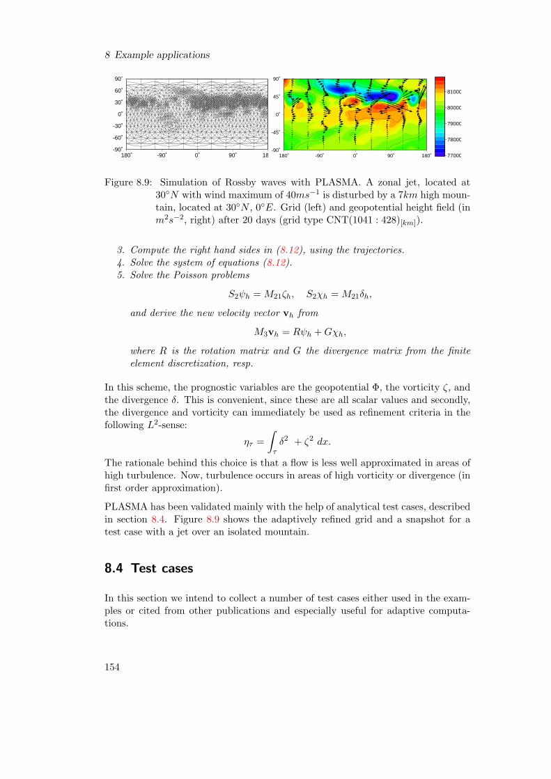
Wolfgang Hiller of Alfred-Wegener-Institute, Bremerhaven, created the scientificfreedom to start with the development of adaptive software for atmospheric model-ing. Natalja Rakowsky (Technische Universitat Hamburg-Harburg, formerly Alfred-Wegener-Institute, Bremerhaven) contributed to the basis of all the numerical imple-mentations, the software package amatos. The development also greatly benefitedfrom Stephan Frickenhaus (Alfred-Wegener-Institute, Bremerhaven) who gave valu-able input in various discussions on the design, Matthias Lauter (Alfred-Wegener-Institute, Potsdam) who was a pilot user with his shallow water model PLASMA,and Thomas Heinze (Deutscher Wetterdienst, formerly TU Munchen), who con-tributed to the spherical version. Matthias Lauter contributed figures 8.9 and8.13.

Many fruitful scientific discussions as well as very nice non-scientific experiences areowed to my friend Francis X. Giraldo from Monterey, CA, USA. In spite of the factthat we did not yet formally collaborate, there is a lot of trust and open exchange ofideas which I regard as exceptional in the scientific community.

Dave Williamson made my visit at NCAR, Boulder, CO, USA, possible and hismentorship was very valuable to me. The inspiring atmosphere in Annick Pouquet’sgroup, including Aime Fournier and Duane Rosenberg, helped to clarify ideas andconcepts. Rich Loft, Stephen Thomas, Ram Nair, Amik St-Cyr among others, allcontributed to the scientifically fruitful stay at NCAR.

I owe gratefulness to Folkmar Bornemann (TU Munchen), who supported my workat TU Munchen tremendously. He also pointed me to the space-filling curves thathelped solve a lot of different technical problems in adaptive implementations. TorSørevik’s (University of Bergen, Norway) support, his invitations to Bergen andthe scientific exchange with him and Ragnhild Blikberg (Paralab, Bergen, Norway)provided inspiration and a productive working atmosphere.

I would like to mention my students that contributed to the results. The originalimplementation of the space-filling code was done by Jens Zimmermann. PhamMinh Bolo and Tobias Landes started the implementation of the 3D version ofamatos, based on the 2D code, while Florian Klaschka developed the algorithmsrelated to the treatment of complex geometries. Florian is also the developer ofVisNET, a visualization package that can easily be combined with amatos. Someof the plots in this work have been made with VisNET. In this context I would liketo acknowledge the use of GMV, the General Mesh Viewer by Frank Ortega, forcreating figures [301]. Lars Mentrup successfully implemented conservative semi-Lagrangian schemes, especially the MPSLM scheme, and elaborated test cases, awork that was prepared by Matthias Dangl.

Many more people influenced my work and I am grateful for the support that I wasgiven. Frank Giraldo, Thomas Heinze, Matthias Lauter, and Lars Mentrup gaveinvaluable input to improve this manuscript.

v

Finally, and most importantly, my family gave me the support and strength to keepthe direction in all these years. I am grateful for the chances that I were offeredand the experience I could gain.

Munich, April 2005Jorn Behrens

vi

Contents

Preface iii

1 Introduction 11.1 Why adaptivity? . . . . . . . . . . . . . . . . . . . . . . . . . . . . . 11.2 Who’s who in adaptive atmospheric modeling . . . . . . . . . . . . . 51.3 Structure of the text . . . . . . . . . . . . . . . . . . . . . . . . . . . 6

2 Principles of adaptive atmospheric modeling 92.1 Paradigms of grid refinement – resolution enhancement versus error

equilibration . . . . . . . . . . . . . . . . . . . . . . . . . . . . . . . . 92.2 Principle difficulties with adaptivity . . . . . . . . . . . . . . . . . . 102.3 Abstract adaptive algorithm . . . . . . . . . . . . . . . . . . . . . . . 122.4 Dynamic grid adaptation – h-refinement . . . . . . . . . . . . . . . . 152.5 Adapting the order of local basis functions – p-refinement . . . . . . 172.6 Refinement criteria . . . . . . . . . . . . . . . . . . . . . . . . . . . . 19

2.6.1 Error proxies . . . . . . . . . . . . . . . . . . . . . . . . . . . 192.6.2 Physics based criteria . . . . . . . . . . . . . . . . . . . . . . 202.6.3 Mathematical error estimation – basic principles . . . . . . . 21

3 Grid generation 253.1 Notation . . . . . . . . . . . . . . . . . . . . . . . . . . . . . . . . . . 253.2 Grid types . . . . . . . . . . . . . . . . . . . . . . . . . . . . . . . . . 283.3 Refinement strategies in 2D . . . . . . . . . . . . . . . . . . . . . . . 303.4 Refinement in 3D . . . . . . . . . . . . . . . . . . . . . . . . . . . . . 413.5 Spherical geometries . . . . . . . . . . . . . . . . . . . . . . . . . . . 44

4 Data structures for computational efficiency 534.1 Data structures for grid management . . . . . . . . . . . . . . . . . . 534.2 Data structures for efficient numerical calculations . . . . . . . . . . 58

4.2.1 Vectorizable data structures . . . . . . . . . . . . . . . . . . . 594.2.2 Maintaining data locality – reordering schemes . . . . . . . . 60

4.3 Working with grid patches . . . . . . . . . . . . . . . . . . . . . . . . 644.4 Software packages for adaptive grid management . . . . . . . . . . . 654.5 Example for a grid handling software package – amatos . . . . . . . 66

vii

Contents

5 Issues in Parallelization of Irregularly Structured Problems 755.1 Metrics for parallelizing irregularly structured problems . . . . . . . 765.2 Partitioning strategies . . . . . . . . . . . . . . . . . . . . . . . . . . 78

5.2.1 Spectral bisection partitioning . . . . . . . . . . . . . . . . . 815.2.2 Kernighan-Lin partitioning . . . . . . . . . . . . . . . . . . . 825.2.3 Multi-level methods . . . . . . . . . . . . . . . . . . . . . . . 835.2.4 Space-filling curves . . . . . . . . . . . . . . . . . . . . . . . . 84

6 Numerical treatment of differential operators on adaptive grids 876.1 Approximating the gradient . . . . . . . . . . . . . . . . . . . . . . . 87

6.1.1 Finite difference approach . . . . . . . . . . . . . . . . . . . . 886.1.2 Least squares approximation . . . . . . . . . . . . . . . . . . 906.1.3 Galerkin approach . . . . . . . . . . . . . . . . . . . . . . . . 906.1.4 Radial basis function approach . . . . . . . . . . . . . . . . . 93

6.2 Evaluating the gradient approximation . . . . . . . . . . . . . . . . . 956.2.1 Further references . . . . . . . . . . . . . . . . . . . . . . . . 97

7 Discretization of conservation laws 1017.1 Some basic mathematical tools . . . . . . . . . . . . . . . . . . . . . 1027.2 Conservation laws of interest . . . . . . . . . . . . . . . . . . . . . . 103

7.2.1 Conservation of mass . . . . . . . . . . . . . . . . . . . . . . . 1047.2.2 Conservation of momentum . . . . . . . . . . . . . . . . . . . 1057.2.3 Conservation of energy . . . . . . . . . . . . . . . . . . . . . . 1077.2.4 Equations of state – closing the system . . . . . . . . . . . . 1087.2.5 Deriving the shallow water equations . . . . . . . . . . . . . . 1097.2.6 The rotating shallow water equations in spherical geometries 111

7.3 Finite volume methods . . . . . . . . . . . . . . . . . . . . . . . . . . 1177.3.1 One-dimensional model problem and basic algorithmic idea . 1177.3.2 Multidimensional extension . . . . . . . . . . . . . . . . . . . 1197.3.3 Convergence, consistency and stability . . . . . . . . . . . . . 121

7.4 Discontinuous Galerkin methods . . . . . . . . . . . . . . . . . . . . 1237.4.1 The basic idea for ordinary differential equations . . . . . . . 1247.4.2 Application of DG methods to multi-dimensional scalar con-

servation laws . . . . . . . . . . . . . . . . . . . . . . . . . . . 1257.5 Conservative semi-Lagrangian methods . . . . . . . . . . . . . . . . . 127

7.5.1 Adaptive semi-Lagrangian scheme . . . . . . . . . . . . . . . 1297.5.2 Mass-conserving algorithms . . . . . . . . . . . . . . . . . . . 132

8 Example applications 1418.1 Tracer advection . . . . . . . . . . . . . . . . . . . . . . . . . . . . . 141

8.1.1 Filamentation of trace gas in the arctic polar vortex . . . . . 1418.1.2 Adaptive tracer transport model . . . . . . . . . . . . . . . . 1428.1.3 Experiments and results . . . . . . . . . . . . . . . . . . . . . 143

8.2 Inverse tracer advection . . . . . . . . . . . . . . . . . . . . . . . . . 146

viii

Contents

8.3 Shallow water equations . . . . . . . . . . . . . . . . . . . . . . . . . 1518.4 Test cases . . . . . . . . . . . . . . . . . . . . . . . . . . . . . . . . . 154

9 Conclusions 1659.1 Evaluation of methods . . . . . . . . . . . . . . . . . . . . . . . . . . 1659.2 Road map for the next five years . . . . . . . . . . . . . . . . . . . . 167

List of notations 173

Bibliography 175

Index 207

ix

Contents

x

List of Figures

1.1 Meteosat satellite image . . . . . . . . . . . . . . . . . . . . . . . . . 21.2 Lee wave cloud pattern . . . . . . . . . . . . . . . . . . . . . . . . . . 31.3 Locally refined grid over Antarctica . . . . . . . . . . . . . . . . . . . 4

2.1 Locally adapted mesh for tracer dispersion . . . . . . . . . . . . . . . 102.2 Locally adapted mesh for error equilibration . . . . . . . . . . . . . . 11

3.1 Hanging nodes . . . . . . . . . . . . . . . . . . . . . . . . . . . . . . 273.2 Bisection of marked edge . . . . . . . . . . . . . . . . . . . . . . . . . 313.3 Iterative refinement by bisection . . . . . . . . . . . . . . . . . . . . 313.4 Admissible patch . . . . . . . . . . . . . . . . . . . . . . . . . . . . . 323.5 Regular triangular refinement . . . . . . . . . . . . . . . . . . . . . . 333.6 Green and blue refinement . . . . . . . . . . . . . . . . . . . . . . . . 333.7 Quadrilateral refinement algorithm . . . . . . . . . . . . . . . . . . . 353.8 Closures for quadrilateral refinement . . . . . . . . . . . . . . . . . . 363.9 Quadrilateral patch refinement . . . . . . . . . . . . . . . . . . . . . 373.10 Closures for quadrilateral patch refinement . . . . . . . . . . . . . . 383.11 Generalization of closures for quadrilateral patches . . . . . . . . . . 383.12 Voronoi cells and Delaunay graph . . . . . . . . . . . . . . . . . . . . 393.13 Delaunay triangulation . . . . . . . . . . . . . . . . . . . . . . . . . . 403.14 Local refinement of Delaunay triangulation . . . . . . . . . . . . . . 413.15 Tetrahedron with marked edge in standard position . . . . . . . . . . 423.16 Bisection of a tetrahedron . . . . . . . . . . . . . . . . . . . . . . . . 423.17 Red and Black tetrahedra . . . . . . . . . . . . . . . . . . . . . . . . 433.18 Hexahedral refinement . . . . . . . . . . . . . . . . . . . . . . . . . . 443.19 Octahedral triangulation of sphere . . . . . . . . . . . . . . . . . . . 473.20 Icosahedral triangulation of sphere . . . . . . . . . . . . . . . . . . . 473.21 Truncated icosahedral triangulation of sphere . . . . . . . . . . . . . 473.22 Lat-Lon and reduced Lat-Lon grid . . . . . . . . . . . . . . . . . . . 503.23 Capped and cubed sphere grids . . . . . . . . . . . . . . . . . . . . . 513.24 Yin Yang grid . . . . . . . . . . . . . . . . . . . . . . . . . . . . . . . 52

4.1 Two phases of an adaptive algorithm . . . . . . . . . . . . . . . . . . 544.2 Example grid with numbered nodes/elements . . . . . . . . . . . . . 554.3 Example of a refinement tree . . . . . . . . . . . . . . . . . . . . . . 58

xi

List of Figures

4.4 Triangular mesh numbering and connectivity matrix . . . . . . . . . 614.5 Cuthill-McKee and minimum degree reordering . . . . . . . . . . . . 624.6 Space filling curve in bisection refinement . . . . . . . . . . . . . . . 634.7 Space filling curve reordering . . . . . . . . . . . . . . . . . . . . . . 64

5.1 Examples of graphs related to meshes . . . . . . . . . . . . . . . . . 805.2 Examples of partitioned adaptively refined meshes . . . . . . . . . . 85

6.1 Piecewise linear basis function bi. . . . . . . . . . . . . . . . . . . . . 926.2 The basic test problem for gradient computation . . . . . . . . . . . 966.3 Convergence of the gradient approximation methods . . . . . . . . . 966.4 Gradient error plots for uniform mesh . . . . . . . . . . . . . . . . . 986.5 Gradient dependence on non-uniformity of mesh . . . . . . . . . . . 986.6 Gradient error plots for non-uniform mesh . . . . . . . . . . . . . . . 986.7 Timing results for the gradient approximation . . . . . . . . . . . . . 99

7.1 Sketch of the shallow water set up. . . . . . . . . . . . . . . . . . . . 1107.2 Idea of the finite volume method . . . . . . . . . . . . . . . . . . . . 1187.3 The dual cell . . . . . . . . . . . . . . . . . . . . . . . . . . . . . . . 1317.4 Upstream dual cell in cell-integrated scheme . . . . . . . . . . . . . . 1347.5 Quadrature points in a triangle . . . . . . . . . . . . . . . . . . . . . 1357.6 Definition of volumes in the MPSLM . . . . . . . . . . . . . . . . . . 1377.7 Mass packet refinement within one cell . . . . . . . . . . . . . . . . . 1387.8 Mass packet mapping step . . . . . . . . . . . . . . . . . . . . . . . . 138

8.1 January monthly mean geopotential (m) for the Arctic . . . . . . . . 1438.2 Adaptively refined grid for advection example . . . . . . . . . . . . . 1448.3 Initial configuration for the artificial model problem . . . . . . . . . 1448.4 Filamentary results of advection with artificial model problem . . . . 1478.5 Initial tracer distribution for the experiments . . . . . . . . . . . . . 1478.6 Tracer concentration using high and low resolution wind data . . . . 1478.7 Tracer concentration for different horizontal resolutions . . . . . . . 1488.8 Inverse tracer advection modeling result . . . . . . . . . . . . . . . . 1518.9 Simulation of Rossby waves with PLASMA . . . . . . . . . . . . . . 1548.10 Accelerating wind test case in 2D . . . . . . . . . . . . . . . . . . . . 1588.11 Accelerating wind test case in 3D . . . . . . . . . . . . . . . . . . . . 1588.12 Initial configuration convergence test case . . . . . . . . . . . . . . . 1598.13 Velocity vectors and geopotential height contours for test case 8.4.8. 162

xii

List of Tables

3.1 Naming convention for adaptive grids . . . . . . . . . . . . . . . . . 29

6.1 Common radial basis functions . . . . . . . . . . . . . . . . . . . . . 95

8.1 Grid resolution and type for advection example . . . . . . . . . . . . 144

xiii

List of Tables

xiv

1 Introduction

Adaptive Modeling in atmospheric sciences has evolved to a state of maturity thatit seems to be the right time to summarize what has been achieved so far andto sketch the near future of research directions. This work gives an overview ofcurrent approaches to adaptive atmospheric modeling. The author has includedmaterial and results cited from other sources in order to give a broader overview ofthe different approaches. It is clear that his own work is described in more detail,even if this might not in all cases be the main-stream in technological development.Many of the achievements of the author’s group are reported in a way that tries tobe as understandable as possible, yet detailed enough to be reproducible. However,if in doubt, readability was given the preference.

In this introductory chapter some motivation for aiming at adaptive atmosphericmodeling is given. This is essentially a collection of arguments, the author cameacross defending his approach against traditionalists especially in the early 1990’swhen adaptive modeling was still a small academic exercise and widely disregarded.However, it is not only a chain of arguments, but also a reasoning, why it mightbe advisable to take the challenge of additional programming complexity, computa-tional overhead and mathematical sophistication to achieve consistent and efficientadaptive models.

When collecting the references, publications and talks on adaptivity, it turns outthat many people did in fact think about adaptive methods for atmospheric prob-lems. So, we give a (certainly not concise) list of people and approaches in adaptiveatmospheric modeling. As a historic remark on adaptive mesh refinement we referto Babuska’s pioneering work [15], which was not related to atmospheric modeling.He coined the term of self-adaptation, which terms a method that adapts itself tothe solution properties, while it computes the solution. We will omit the prefix“self” and call such methods adaptive methods.

1.1 Why adaptivity?

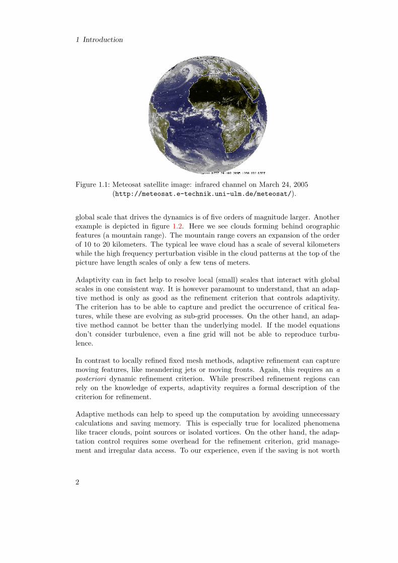
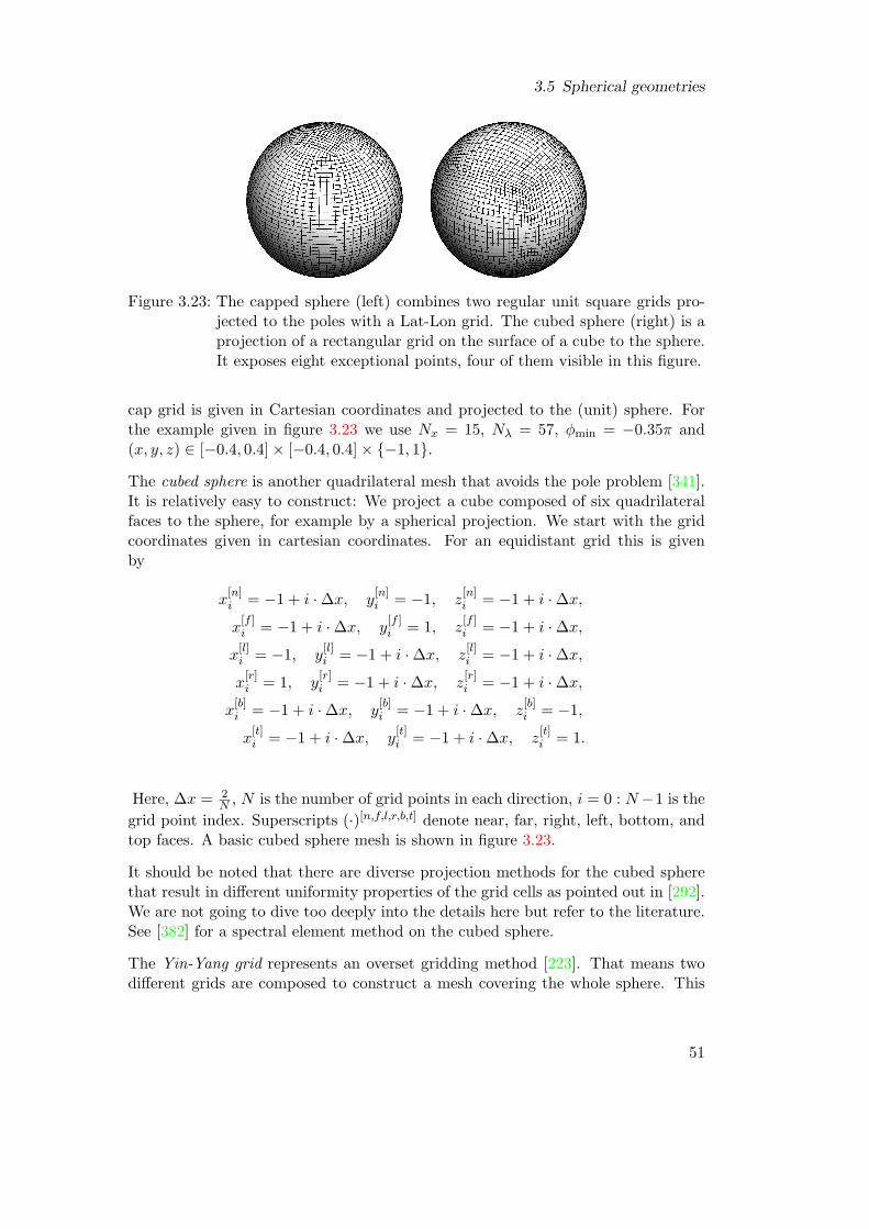
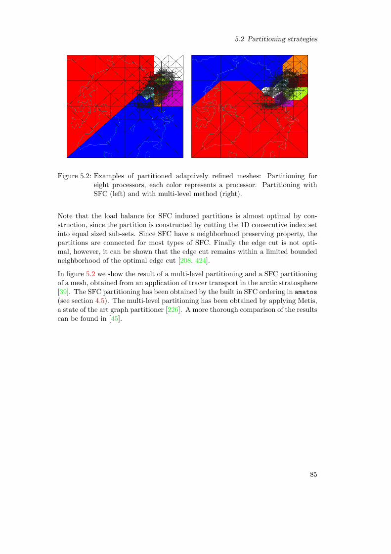
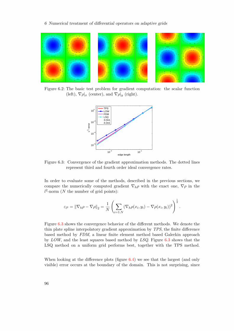
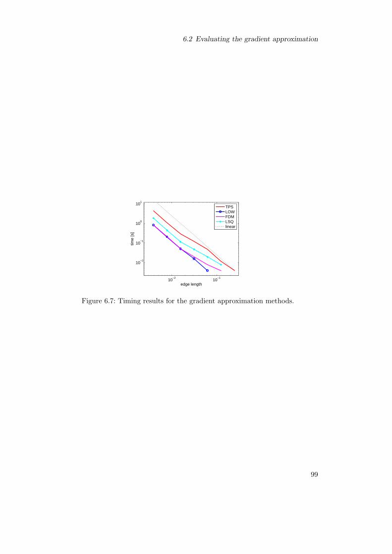
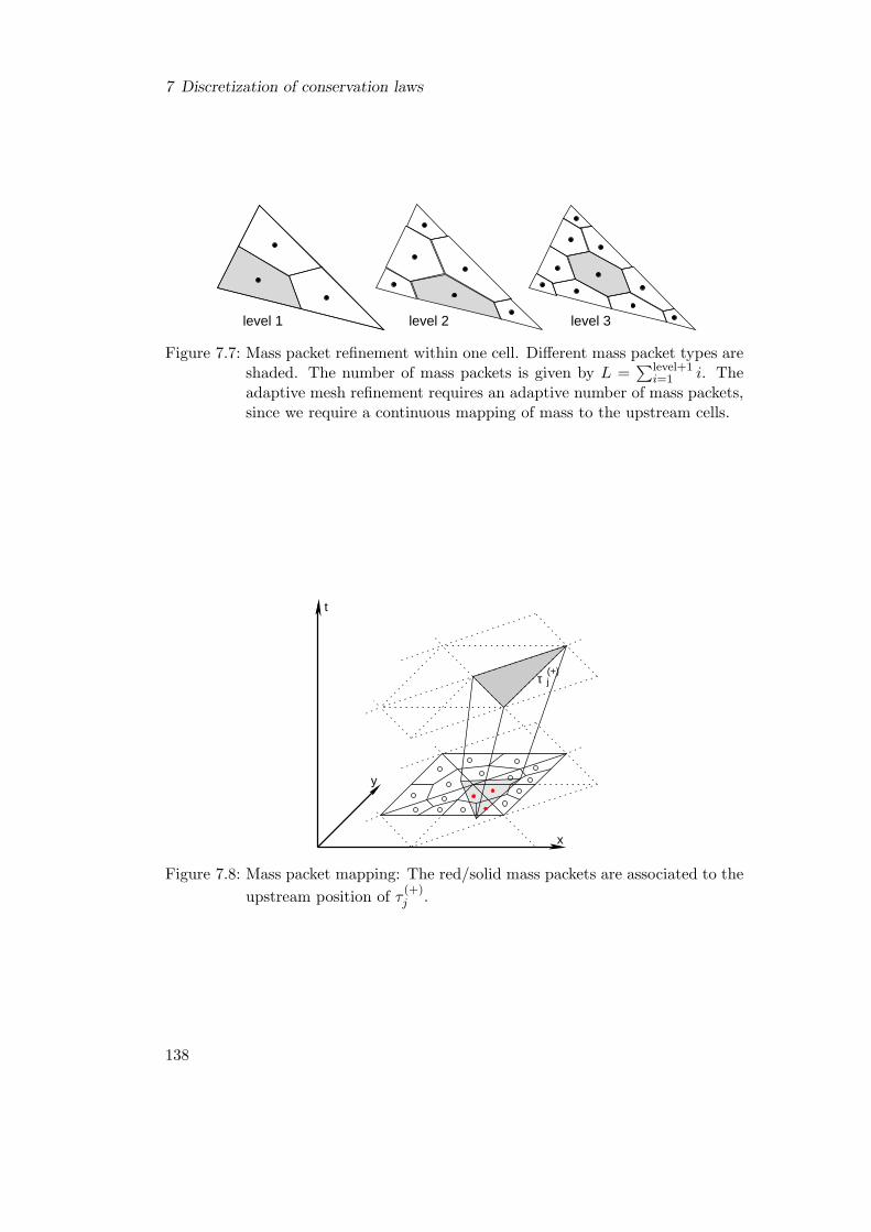
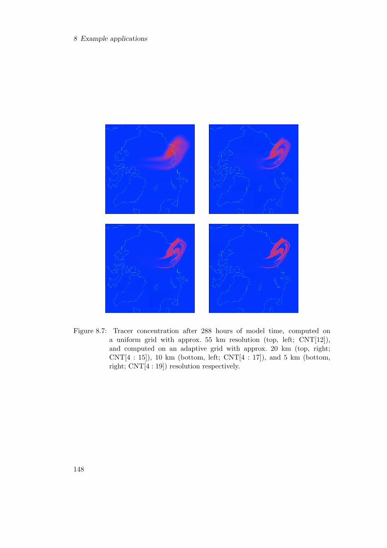
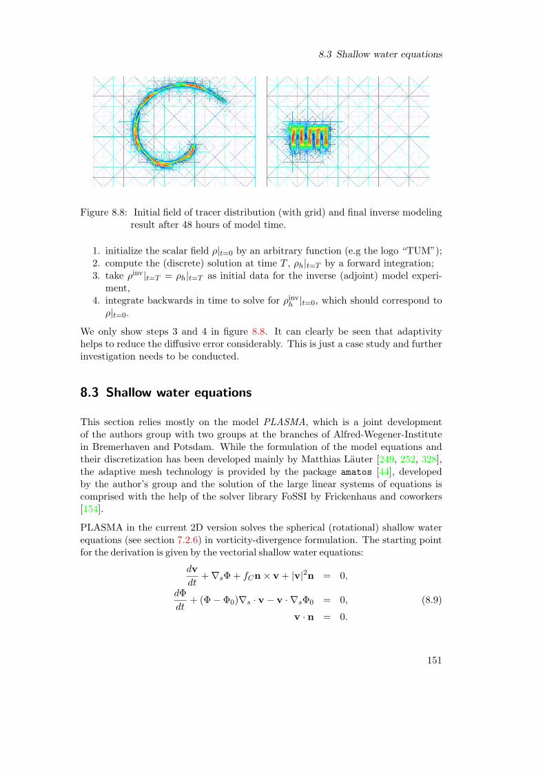
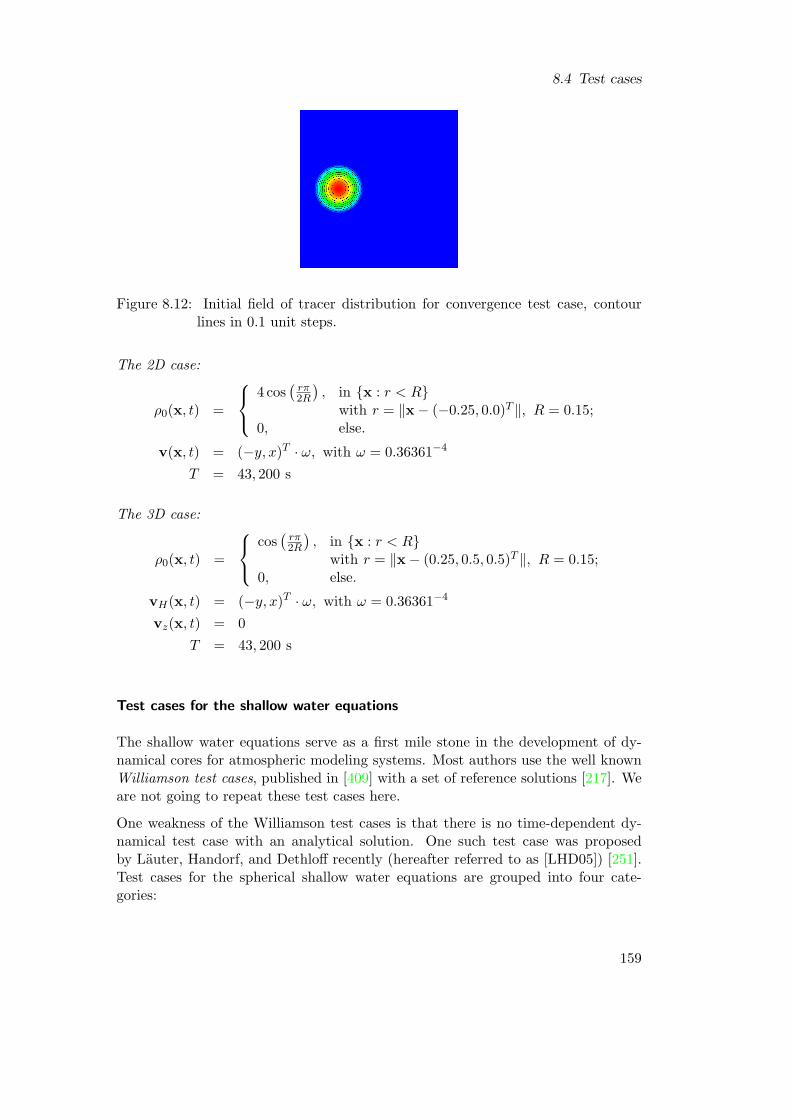
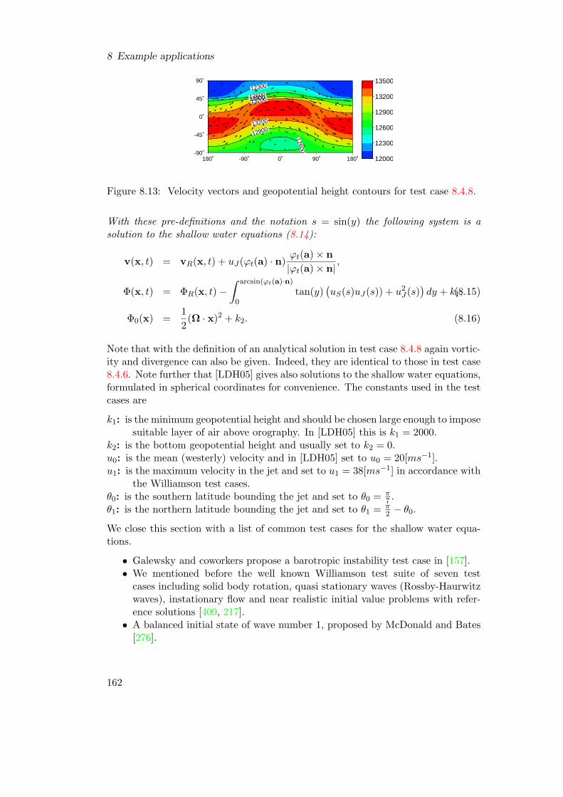
When looking at atmospheric phenomena, one almost always observes interaction ofa variety of scales. Looking at a satellite image (figure 1.1), one can observe fine scalestructures like a cyclone over the Atlantic ocean with filamentary structures andfronts that comprise a relevant length scale of approximately 5 to 10 km, while the

1

1 Introduction

Figure 1.1: Meteosat satellite image: infrared channel on March 24, 2005(http://meteosat.e-technik.uni-ulm.de/meteosat/).

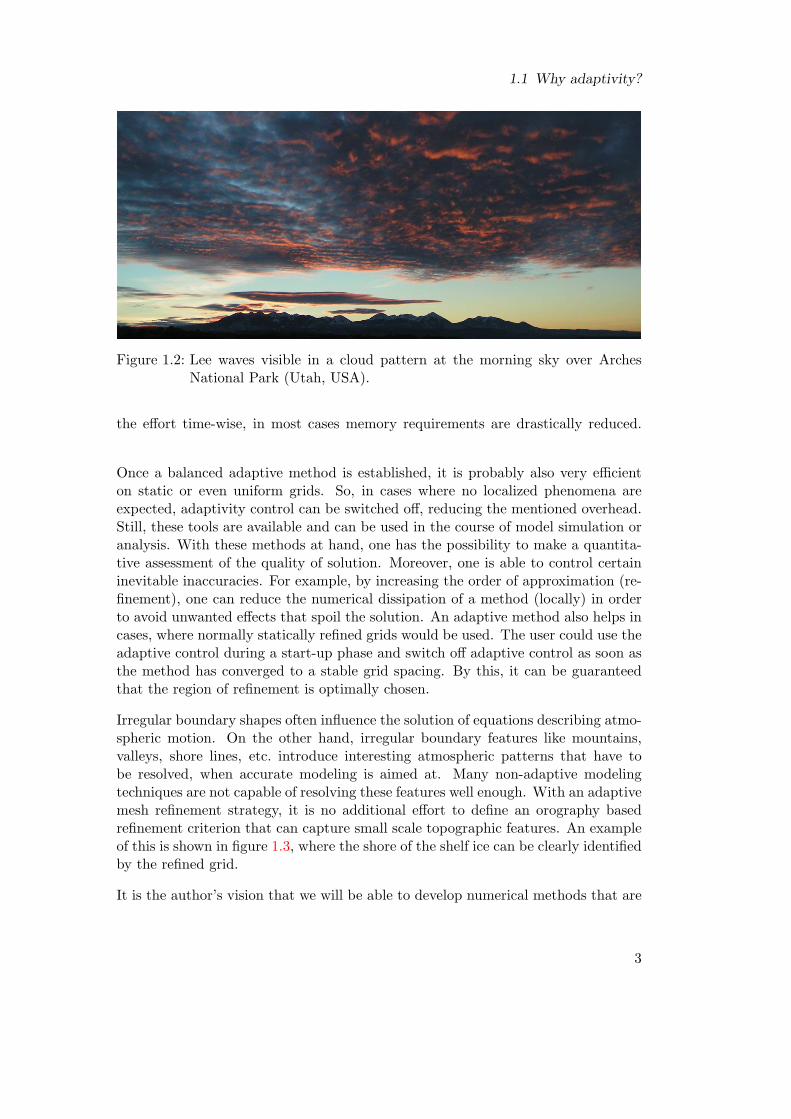
global scale that drives the dynamics is of five orders of magnitude larger. Anotherexample is depicted in figure 1.2. Here we see clouds forming behind orographicfeatures (a mountain range). The mountain range covers an expansion of the orderof 10 to 20 kilometers. The typical lee wave cloud has a scale of several kilometerswhile the high frequency perturbation visible in the cloud patterns at the top of thepicture have length scales of only a few tens of meters.

Adaptivity can in fact help to resolve local (small) scales that interact with globalscales in one consistent way. It is however paramount to understand, that an adap-tive method is only as good as the refinement criterion that controls adaptivity.The criterion has to be able to capture and predict the occurrence of critical fea-tures, while these are evolving as sub-grid processes. On the other hand, an adap-tive method cannot be better than the underlying model. If the model equationsdon’t consider turbulence, even a fine grid will not be able to reproduce turbu-lence.

In contrast to locally refined fixed mesh methods, adaptive refinement can capturemoving features, like meandering jets or moving fronts. Again, this requires an aposteriori dynamic refinement criterion. While prescribed refinement regions canrely on the knowledge of experts, adaptivity requires a formal description of thecriterion for refinement.

Adaptive methods can help to speed up the computation by avoiding unnecessarycalculations and saving memory. This is especially true for localized phenomenalike tracer clouds, point sources or isolated vortices. On the other hand, the adap-tation control requires some overhead for the refinement criterion, grid manage-ment and irregular data access. To our experience, even if the saving is not worth

2

1.1 Why adaptivity?

Figure 1.2: Lee waves visible in a cloud pattern at the morning sky over ArchesNational Park (Utah, USA).

the effort time-wise, in most cases memory requirements are drastically reduced.

Once a balanced adaptive method is established, it is probably also very efficienton static or even uniform grids. So, in cases where no localized phenomena areexpected, adaptivity control can be switched off, reducing the mentioned overhead.Still, these tools are available and can be used in the course of model simulation oranalysis. With these methods at hand, one has the possibility to make a quantita-tive assessment of the quality of solution. Moreover, one is able to control certaininevitable inaccuracies. For example, by increasing the order of approximation (re-finement), one can reduce the numerical dissipation of a method (locally) in orderto avoid unwanted effects that spoil the solution. An adaptive method also helps incases, where normally statically refined grids would be used. The user could use theadaptive control during a start-up phase and switch off adaptive control as soon asthe method has converged to a stable grid spacing. By this, it can be guaranteedthat the region of refinement is optimally chosen.

Irregular boundary shapes often influence the solution of equations describing atmo-spheric motion. On the other hand, irregular boundary features like mountains,valleys, shore lines, etc. introduce interesting atmospheric patterns that have tobe resolved, when accurate modeling is aimed at. Many non-adaptive modelingtechniques are not capable of resolving these features well enough. With an adaptivemesh refinement strategy, it is no additional effort to define an orography basedrefinement criterion that can capture small scale topographic features. An exampleof this is shown in figure 1.3, where the shore of the shelf ice can be clearly identifiedby the refined grid.

It is the author’s vision that we will be able to develop numerical methods that are

3

1 Introduction

Figure 1.3: Locally and statically refined grid over Antarctica, the topography gra-dient has been used as a refinement criterion.

robust and efficient enough to be combined with adaptivity in standard (operational)environments in atmospheric research. When we look at the development of numeri-cal methods for ordinary differential equations (see for example [118, 119, 178, 179])we see that today it is just a standard to use adaptive integrators. These methodshave reached a state of maturity that nobody really thinks about grids and adap-tive control anymore, but the user decides on accuracy and the software fulfills theneeds. This is the vision of adaptive atmospheric modeling (and probably adaptivesolution of PDEs in general).

Thus, adaptivity triggers the concern about accuracy and local error much morethan non-adaptive methods do. Once there is control over local approximation or-der, one has to decide on a tolerable error measure. At that point the question ariseson what “error” really means in a fully equipped atmospheric model.

To summarize, the promise of adaptive atmospheric modeling is the

• locally accurate• efficient• error controlled• truly multi-scale

simulation of atmospheric processes.

4

1.2 Who’s who in adaptive atmospheric modeling

1.2 Who’s who in adaptive atmosphericmodeling

Early approaches to adaptive mesh refinement in atmospheric modeling were pre-sented by researchers in Hurricane or Typhoon prediction that nested finer meshesinto coarse mesh models of the large scale simulation. One example of this not yetadaptive approach is documented in [260]. Others are given in [242, 243]. Nesting isstill a wide spread technique for achieving local high resolution [155]. However, thisreview is concerned with adaptive methods, which means methods that dynamicallyadapt to flow features during run time.

Early truly adaptive models were developed by Klemb and Skamarock and by Di-etachmayer and Droegemeier [123, 362, 364]. Klemb and Skamarock based theirrefinement strategy on a truncation error estimate [269].

There are two major adaptation principles, discussed in section 2.4. One does notchange the grid topology (i.e. the number of grid points and the inter-connectivity)but changes the spacing between grid points by transformation functions [70]. Theother principle refines/coarsens the mesh by inserting/deleting grid points and re-meshing (locally). Examples for the first approach are given in [123] and morerecently in [77, 210]. The author’s work and much of what follows in this book,follows the second approach.

The first – and to the author’s knowledge only – adaptive and operational weatherand dispersion model OMEGA uses a finite volume approach on an unstructuredDelaunay mesh that is locally modified and smoothed [20, 170]. OMEGA has beendeveloped by Bacon and coauthors at Science Applications International Corp.,McLean, VA. Giraldo based at Naval Research Lab in Monterey, CA, has usedDelaunay meshes for adaptively refined Lagrange-Galerkin methods to solve theshallow water equations [162]. Recently, a nodal spectral element method for tri-angular adaptively refined meshes has been proposed [167]. Iselin and coauthorspublished a dynamically adaptive version of the MPDATA scheme [210, 209]. MP-DATA is a finite difference scheme that has several advantageous characteristicslike conservation properties. Prusa and Smolarkiewicz combine a dynamic gridadaptation (movement) method with an Eulerian or semi-Lagrangian conservativeadvection scheme in [326]. Recently, Smolarkiewicz and Szmelter have presented anunstructured grid formulation of MPDATA [367]. There are several groups involvedin adaptive air quality modeling [368, 235, 310].

Jablonowsky’s dissertation, defended at the University of Michigan, is an example ofa finite volume scheme on quadrilateral adaptively refined meshes applied to the 2Dshallow water equations and the 3D baroclinic equations on the sphere [216]. Addi-tionally, she gives a good introduction to adaptive methods in atmospheric modeling.Barros and Garcia recently introduced a variable resolution semi-Lagrangian modelfor global circulation with the shallow water equations [26]. Fiedler uses dynamic

5

1 Introduction

grid adaptation to resolve the boundary layer [144]. A wavelet approach has beenutilized in adaptive ocean modeling in [218].

In the UK a strong adaptive tradition in atmospheric modeling is represented byworks of Tomlin and coworkers. A fully 3D approach on unstructured tetrahedralmeshes is documented in [388] and [161]. Hubbart and Nikiforakis use a 3D quadri-lateral locally refined mesh for simulating global tracer transport in [202]. For theocean Pain, Ford, Piggott and coworkers developed an advanced adaptive modelingtool for 3D unstructured computations [149, 150, 304, 317].

Ivanenko and Muratova introduce a quadrilateral distorted grid based finite differ-ence shallow water model with local mesh refinement [215]. Blayo and Debreu uselocal mesh refinement in the context of finite difference methods for ocean modeling[61]. Kashiyama and Okada use adaptive mesh generation techniques for solvingshallow water flow problems [231]. Again in ocean modeling an adaptive 3D shallowwater model has been proposed by Ham and coworkers in the Netherlands [181].Hundsdorfer et al. proposed an adaptive method of lines based finite differenceapproach for atmospheric transport problems [207].

In Germany the author’s group is active since the early 1990’s in adaptive at-mospheric modeling [33, 34, 35, 36, 39]. Lauter introduced a shallow water modelin vorticity-divergence formulation on the sphere [249, 250]. Hess has developed anadaptive and parallel multi-grid solver for the shallow water equations [196].

To summarize, research in adaptive atmospheric (and ocean) modeling is gainingmomentum in recent years. This is documented in a study on numerical schemes fornon-hydrostatic models that explicitly addresses suitability of schemes to adaptivelyrefined meshes [371]. However, the group of people working on adaptive modelingin this field is still moderate, even if one takes into account that the above list iscertainly not complete.

1.3 Structure of the text

This work is intended to give an overview of adaptive atmospheric modeling tech-niques in a way that makes it possible to extract the basic ideas for the own devel-opment, together with additional pointers to the more detailed literature. Severalaspects are covered in more detail. At the end of this book, a reader should be able todraft a simple adaptive atmospheric modeling technique for his/her own needs andfind literature with detailed descriptions on the construction.

Chapter 2 introduces several principles of adaptive modeling. It is of a more ab-stract and basic character, since adaptive methods are not well established in theatmospheric modeling community yet.

6

1.3 Structure of the text

In chapter 3 grid generation techniques are covered in some detail. Grid refine-ment is the major tool for multi-scale adaptivity in atmospheric modeling to date.Therefore, some effort has been put into the compilation of 2D and 3D triangular(unstructured) and quadrilateral (structured) mesh refinement strategies. Addition-ally basic initial grids for spherical geometries are introduced.

Computational aspects are treated in chapter 4. Grid generation – especially forunstructured grids – needs adequate data structures. On the other hand, numericalalgorithms need consecutive data structures for efficient execution. Both require-ments are covered there.

Chapter 5 treats issues in parallelization. Efficient execution on modern computingarchitectures calls for parallelizable data structures and dynamic load balancing.In this regard, chapters 4 and 5 are interrelated. While the description in theformer is valid for uniprocessor architectures alike, the latter is only valid for parallelarchitectures.

Chapters 6 and 7 deal with the more mathematical aspects of adaptive modeling:the representation of differential operators on adaptive grids and the discretizationof conservation laws. While conservation laws are the basic equations relevant inatmospheric modeling, they are mostly given in terms of partial differential equa-tions. Thus, the discretization of conservation laws requires differential operatorsto be represented on adaptive meshes.

Chapter 8 gives examples of the successful application of adaptive methods to at-mospheric modeling. Additionally, test cases for studying basic properties of adap-tive methods are introduced.

In 9 we draw conclusions from the material in the previous chapters and try to derivebasic rules of good practice. Finally, we try to pave the way to the future of adaptivetechniques in atmospheric modeling. It is the authors belief that adaptivity is abasic principle of multi-scale processes. Therefore, adaptive techniques will help tounderstand and solve future problems in atmospheric modeling.

7

1 Introduction

8

2 Principles of adaptive atmosphericmodeling

In this chapter, major principles of adaptivity and especially adaptive atmosphericmodeling will be discussed. We start with reconsidering the paradigms of adaptivityin the mathematical and in the meteorological communities respectively in order toclarify the basic notations. After this clarification, and a description of principlechallenges in adaptivity, we introduce concepts of adaptive refinement techniquesand discuss refinement criteria.

2.1 Paradigms of grid refinement – resolution enhancementversus error equilibration

A common cause for misunderstanding when talking about adaptive mesh refine-ment, or adaptivity in general, is the existence of two different approaches. In orderto avoid ambiguity or confusion this section explains the two paradigms.

The first approach is interested in increasing resolution locally. This is the prevailingaim in most meteorological applications, and fixed local mesh refinement has longbeen used to achieve this goal (see for example [100, 115]). The approach is drivenby the physical understanding that increased resolution reveals more structure inthe simulated phenomena.

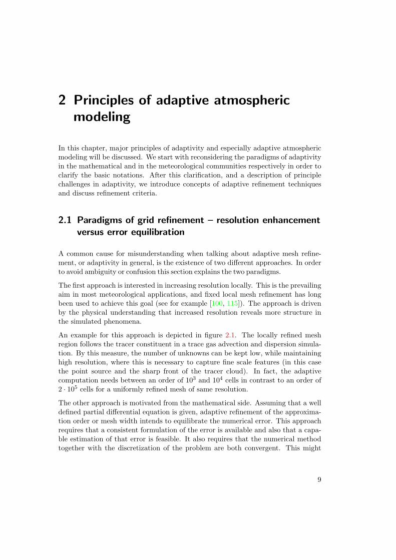
An example for this approach is depicted in figure 2.1. The locally refined meshregion follows the tracer constituent in a trace gas advection and dispersion simula-tion. By this measure, the number of unknowns can be kept low, while maintaininghigh resolution, where this is necessary to capture fine scale features (in this casethe point source and the sharp front of the tracer cloud). In fact, the adaptivecomputation needs between an order of 103 and 104 cells in contrast to an order of2 · 105 cells for a uniformly refined mesh of same resolution.

The other approach is motivated from the mathematical side. Assuming that a welldefined partial differential equation is given, adaptive refinement of the approxima-tion order or mesh width intends to equilibrate the numerical error. This approachrequires that a consistent formulation of the error is available and also that a capa-ble estimation of that error is feasible. It also requires that the numerical methodtogether with the discretization of the problem are both convergent. This might

9

2 Principles of adaptive atmospheric modeling

Figure 2.1: Locally adapted meshes for tracer dispersion experiment over SouthernGermany, Four time steps are shown, starting from a point source.

not be the case in real life meteorological applications, where discrete models ofsub-grid processes can destroy convergence.

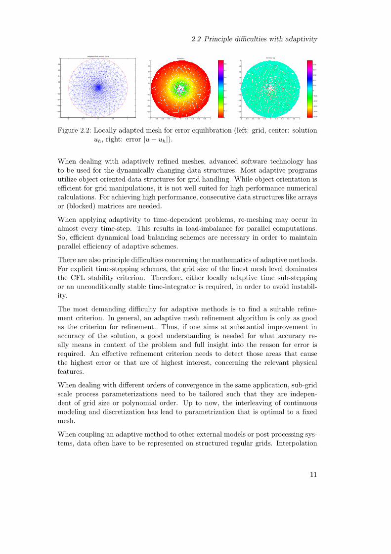
This paradigm was introduced in the early 1970’s probably by Babuska [15, 18]. Itwas originally used with finite element methods (FEM). For a historical draft of thedevelopment of FEM see [89, 384]. An example is depicted in figure 2.2, namely thesolution of Poisson’s equation on a circular domain with a Dirac delta function load(right hand side). This example is taken from the MATLAB PDE toolbox demos[271].

In many cases the two approaches will find similar solutions. Since intuitively, areasof high physical activity will be those of high mathematical error (e.g. steep gra-dient regions, high local curvature of some constituent). However, there are cases,where the mathematically induced error-driven criterion refines counter-intuitively.This statement is especially valid for transport dominated problems, found in at-mospheric modeling, since error can be propagated and the propagation directionmay not be predictable. In general, refinement criteria are very problem dependentand have to be chosen after a careful analysis of the problem’s requirements (see sec-tion 2.6 for a more detailed description of refinement criteria).

2.2 Principle difficulties with adaptivity

While an adaptive method promises to be more efficient for certain cases of localizedfeatures, it incurs several new difficulties that need to be treated with care. Somedifficulties can be circumvented by reasonable choices of software methods, othersneed to be tackled by mathematically more sophisticated methods. This sectionlists some of the principle difficulties that will be treated in the course of thispresentation.

Let us first look at the computer science part of adaptive methods. Since locallyrefined meshes are mostly unstructured, indirect addressing and the correspondingperformance loss is an issue. Even in the case of locally structured grids, an overheadof address information has to be taken into account.

10

2.2 Principle difficulties with adaptivity

−1 −0.5 0 0.5 1−1

−0.8

−0.6

−0.4

−0.2

0

0.2

0.4

0.6

0.8

1Adaptive Mesh on Unit Circle

−1 −0.8 −0.6 −0.4 −0.2 0 0.2 0.4 0.6 0.8 1−1

−0.8

−0.6

−0.4

−0.2

0

0.2

0.4

0.6

0.8

1Solution u

0

0.1

0.2

0.3

0.4

0.5

0.6

0.7

0.8

−1 −0.8 −0.6 −0.4 −0.2 0 0.2 0.4 0.6 0.8 1−1

−0.8

−0.6

−0.4

−0.2

0

0.2

0.4

0.6

0.8

1

Error |u−uh|

−0.05

−0.04

−0.03

−0.02

−0.01

0

0.01

0.02

0.03

0.04

0.05

Figure 2.2: Locally adapted mesh for error equilibration (left: grid, center: solutionuh, right: error |u− uh|).

When dealing with adaptively refined meshes, advanced software technology hasto be used for the dynamically changing data structures. Most adaptive programsutilize object oriented data structures for grid handling. While object orientation isefficient for grid manipulations, it is not well suited for high performance numericalcalculations. For achieving high performance, consecutive data structures like arraysor (blocked) matrices are needed.

When applying adaptivity to time-dependent problems, re-meshing may occur inalmost every time-step. This results in load-imbalance for parallel computations.So, efficient dynamical load balancing schemes are necessary in order to maintainparallel efficiency of adaptive schemes.

There are also principle difficulties concerning the mathematics of adaptive methods.For explicit time-stepping schemes, the grid size of the finest mesh level dominatesthe CFL stability criterion. Therefore, either locally adaptive time sub-steppingor an unconditionally stable time-integrator is required, in order to avoid instabil-ity.

The most demanding difficulty for adaptive methods is to find a suitable refine-ment criterion. In general, an adaptive mesh refinement algorithm is only as goodas the criterion for refinement. Thus, if one aims at substantial improvement inaccuracy of the solution, a good understanding is needed for what accuracy re-ally means in context of the problem and full insight into the reason for error isrequired. An effective refinement criterion needs to detect those areas that causethe highest error or that are of highest interest, concerning the relevant physicalfeatures.

When dealing with different orders of convergence in the same application, sub-gridscale process parameterizations need to be tailored such that they are indepen-dent of grid size or polynomial order. Up to now, the interleaving of continuousmodeling and discretization has lead to parametrization that is optimal to a fixedmesh.

When coupling an adaptive method to other external models or post processing sys-tems, data often have to be represented on structured regular grids. Interpolation

11


onto such interface grids needs to be consistent with the modeling error and con-servation properties of the physical constituents that are communicated (e.g. fluxeshave to adhere to mass conservation).

2.3 Abstract adaptive algorithm

In this section we will introduce an abstract formulation of the adaptive algorithmfor atmospheric transport-dominated problems. This algorithm is based on a pos-teriori refinement criteria. We will also define basic notations.

It is important to distinguish between a priori and a posteriori error control. Whilea priori refinement criteria where used even in the very first paper describing finite el-ement methods [391], a posteriori error control is a later concept.

With a priori error control or a priori refinement criteria we denote those methodsthat have prior knowledge about the solution of the problem and react by refiningthe approximation accordingly. Examples of this are models that refine over areasof interest [100, 115, 281], or in areas of known high turbulent activity, e.g. nearsteep topographical features (mountains, sea mounts, valleys, etc.) [90, 105, 150,181, 420].

For an adaptive algorithm, some kind of a posteriori refinement criterion is neces-sary. The algorithm starts with solving the problem on a provisional grid. Then,a posteriory (i.e. after solving), a criterion determines those regions of the compu-tational domain that need to be refined. Finally, a new solution is computed on therefined grid.

In general the true error is not available during the computation. So, for a math-ematical determination of refinement areas, i.e. areas of large local error, an errorestimator is needed. The concept of self-adaptation has been coined by Babuska[15]. The mathematical error estimation approach requires deep theoretical insightinto the nature of error of the numerical method together with the problem to besolved.

A posteriori refinement control can also be derived from heuristical criteria. In manycases gradients of relevant physical quantities or curvature properties are used forrefinement. It is also possible to use proxy data in order to obtain a refinementcriterion. So, even without deep theoretical error analysis, and even without aclear concept of error, an abstract a posteriori adaptively refined algorithm can beformulated.

Before stating the adaptive algorithm, the basic non-adaptive algorithm should beformulated. For transport dominated atmospheric flow problems, it is assumed thata discretization of the governing equations is performed in space and time separately.

12

2.3 Abstract adaptive algorithm

Thus, we first semi-discretize in time to obtain a time-stepping scheme, and thendiscretize the remaining stationary problem in space.

Let us assume that the time interval of interest I is normalized to start at time0, I = [0, T ] ∈ R. Let us denote the spatial domain with G ⊂ Rd and denoteρh the discrete variable corresponding to the continuous variable ρ. In general,ρ defines a map ρ : G × I → Rr, where r = 1 for scalar and r = d for vector-valued variables. Then ρh defines a map ρh : Gh × Ih → Rr. Here Gh is somediscrete representation of G, for example a polygonal approximation of the truedomain, which can be discretized by a triangulation T = τ1, . . . , τM (see section3.1 for a formal definition of a triangulation). Ih is the discretized time intervalIh = ti : 0 ≤ ti ≤ T (i = 0 : K). If we deal with systems then ρ and ρhrepresent vectors of all prognostic variables. We formulate the abstract problem bythe following equation

∂

∂tρ+Dρ = r, (2.1)

with a differential operator D = D(t,x, ρ) and a right hand side r = r(t,x, ρ).Additionally initial values ρ(t = 0) = ρ0 and boundary values ρ(t)|∂G = ρb(t) areassumed to be given. Furthermore, we assume that the time derivative can berepresented as an evolution

ρ(t > 0) = Ψ(0, t; ρ(0)),

and that the stationary problem can be solved separately and is represented by

Dξ = r,

where ξ can then be used in the evolution, ρ(t > 0) = Ψ(0, t; ξ). With theseassumptions, the basic non-adaptive algorithm reads as follows

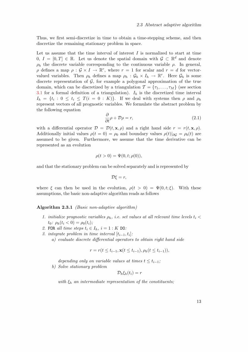
Algorithm 2.3.1 (Basic non-adaptive algorithm)

1. initialize prognostic variables ρh, i.e. set values at all relevant time levels ti <t0: ρh(ti < 0) = ρ0(ti);

2. FOR all time steps ti ∈ Ih, i = 1 : K DO:3. integrate problem in time interval [ti−1, ti]:

a) evaluate discrete differential operators to obtain right hand side

r = r(t ≤ ti−1,x(t ≤ ti−1), ρh(t ≤ ti−1)),

depending only on variable values at times t ≤ ti−1;b) Solve stationary problem

Dhξh(ti) = r

with ξh an intermediate representation of the constituents;

13


c) update prognostic variables at time ti:

ρh(ti) = Ψh(ti, ti−1; ξh(t ≤ ti−1)),

where Ψh is the discrete evolution operator;4. perform any other diagnostic calculations depending on values ρh(ti);5. END DO.

Remark 2.3.2 Note that algorithm 2.3.1 tries to be rather general. For example,an explicit method would have a diagonal system matrix Sh = diag(sh), where sh is avector of coefficients. However, this algorithm does not cover all possible discretiza-tion schemes for PDEs as they occur in atmospheric modeling, because it assumesthat the discretization leads to a time stepping scheme and that an evolution operatorcan be derived from the system of equations.

With this formal abstract definition of a time-stepping algorithm, it requires justtwo additional steps to define a basic adaptive algorithm:

Algorithm 2.3.3 (Basic adaptive algorithm)

1. initialize prognostic variables ρh (as in algorithm 2.3.1);2. FOR all time steps ti ∈ Ih, i = 1 : K DO:3. integrate problem in time interval [ti−1, ti]:

a) evaluate discrete differential operators to obtain right hand side

r = r(t ≤ ti−1,x(t ≤ ti−1), ρh(t ≤ ti−1)),

depending only on variable values at times t ≤ ti−1;b) Solve stationary problem

Dhξh(ti) = r

with ξh an intermediate representation of the constituents;c) update prognostic variables at time ti:

ρh(ti) = Ψh(ti, ti−1; ξh(t ≤ ti−1)),

where Ψh is the discrete evolution operator;d) calculate local refinement criterion ητ for each τ ∈ T , and refine those

τ , where ητ > θref , with θref a given refinement tolerance;e) IF grid changed, THEN: return to step 3a, ELSE: continue with step 4;

4. perform any other diagnostic calculations depending on values ρh(ti);5. END DO.

Note that only steps 3d and 3e in algorithm 2.3.3 have been added to the originalbasic algorithm 2.3.1. However, in these two steps, a huge amount of computationalintelligence is involved. We will specify the details of the refinement strategy insections 2.4 and 2.5 below. Furthermore, grid refinement in geometric terms isdiscussed in chapter 3, while some remarks on refinement criteria are made in section2.6.

14

2.4 Dynamic grid adaptation – h-refinement

2.4 Dynamic grid adaptation – h-refinement

One principle of adaptivity is to refine the computational mesh. This will be thepredominant method throughout this text. Commonly, the spatial mesh size isdenoted by h, therefore, refining the mesh corresponds to refining h. So, a commonname for adaptive mesh refinement (AMR) in the mathematical community is h-refinement.

h-refinement is based on an approximation property of the kind

εh = ‖ρ− ρh‖ ≤ Chν ‖ρ‖ , (2.2)

where we denote by ρ the true solution of some given problem, ρh is a discrete ap-proximation, C is a constant, h is a parameter indicating the mesh width, andν is the order of convergence. Equation (2.2) states that for h → 0 the dis-crete solution ρh tends to the true solution ρ or in other words, the error εh →0.

In the following we want to denote by

• εh the discretization error: εh = ‖ρ− ρh‖ in an appropriate norm;• ετ the local discretization error εh|τ ;• [εh], and [ετ ] an estimation of the global and local discretization error, resp.;• ητ or ηi for each τi, a local criterion that can be an error estimate or some

other local measure that can be used to derive a refinement.

There are several strategies to select the refinement regions. Ultimately, one is inter-ested in getting the most accurate solution with least effort. Therefore, an algorithmfor refinement has to be given. For now, let us assume that we can compute a localerror, denoted by ετ (we will present common error estimators and refinement cri-teria in section 2.6). A first simple approach is based on the maximum norm of thelocal error vector εm := (ετ1 , . . . , ετm). With εh = εmax = ‖εm‖∞ = maxk=1:m ετkthe global error in the∞-norm, one can try to minimize the global error by refiningthose elements of the mesh that have largest local errors.

More precisely, with a given tolerance 0 ≤ θref ≤ 1, a simple algorithm for localmesh refinement is given by

Algorithm 2.4.1 (∞-Norm based h-refinement)

1. Let T0 be a given initial triangulation, ε0 the vector of local error componentsετi, i = 1 : m, and ε0max =

∥∥ε0∥∥∞.2. FOR all τ ∈ T0 DO:3. IF ετ > θrefε

0max THEN:

a) refine τ4. END DO.

15


While algorithm 2.4.1 is scaling invariant (i.e. if ε0 is multiplied by a scalar α,then the result of refinement does not change) and extremely simple, there is in factno theoretical guarantee, that the discretization error is always reduced, or thatan algorithm equipped with this refinement procedure really converges. However,in practical applications this strategy has been used successfully (see [39] for itsapplication in a tracer transport problem).

Another p-norm based approach is the so called equi-distribution strategy [137]. Itis best illustrated by assuming a uniform distribution of local errors ετ = ε forall τ ∈ T0. Now, we define the global error to be the p-norm of the local errorvector:

ε = ‖εm‖p =

( ∑k=1:m

εpτk

) 1p

= (mεp)1p = m

1p ε.

We require ε ≤ θref . If we let ε = θref , we can see that ε = θref

m1p. From this, we

derive the heuristic

Algorithm 2.4.2 (equi-distribution h-refinement)

1. Let T0 be a given initial triangulation.2. FOR all τ ∈ T0 DO:3. IF ετ >

θref

m1pTHEN:

a) refine τ4. END DO.

Lauter uses this strategy for p = 2 in an application to adaptive shallow watermodeling in [250].

Dorfler introduces a guaranteed error reduction strategy [126]. This strategy – onlyoutlined here, since it is hardly ever used in atmospheric modeling so far – is basedon the idea that a subset of mesh elements is refined with the sum of their localerrors being a fixed part of the total error ε. Thus, given a parameter 0 < θ < 1,find a minimal set S = τ1, . . . , τk ⊆ T0, such that∑

τ∈Sεpτ ≥ (1− θ)pεp. (2.3)

It follows that if S is being refined, the error will be reduced by a factor depending onθ and the properties of the problem data (right hand side, etc.). Dorfler proposes astrategy for selecting the elements in S by an inner iteration. In this inner iteration,the ∞-norm strategy 2.4.1 is used with a decreasing threshold θref until S is largeenough to meet the requirement in (2.3).

So far, only refinement strategies have been considered. In transport dominatedatmospheric modeling the area of interest may move over time, so that we may

16

2.5 Adapting the order of local basis functions – p-refinement

need to coarsen the mesh after a while. Both of the above strategies 2.4.1 and2.4.2 can be inverted easily to be used as coarsening strategies. As an example, wedemonstrate this for the ∞-norm strategy 2.4.1. Let 0 ≤ θcrs < θref . Then one maycoarsen an element τ of the triangulation if

ετ < θcrsε0max.

There are two topics that have to be kept in mind. First, the choice of θcrs has to bedone carefully in order to avoid incompatible refinement and coarsening conditions.These in turn can cause oscillating refinement/coarsening of single elements. Inmathematical a posteriori error estimation, one can usually give an approximationof ετ in terms of the element (mesh) width hτ :

ετ ≤ Chντ ,

where ν is an appropriate exponent. For linear approximation order (ν = 1), coars-ening the element such that the mesh width is doubled, causes the local error toincrease by a factor of 2. Therefore, we have to choose

θcrs ≤θref2,

in order to avoid oscillatory behavior. For higher approximation order this argumenthas to be modified appropriately.

Secondly, we need to define a coarsening strategy, since an element can only be coars-ened, if the corresponding siblings are also coarsened. This strategy is described insection 3 in connection with the refinement strategies.

2.5 Adapting the order of local basis functions –p-refinement

In contrast to the h-refinement of the previous section, where the grid is refined,one can also increase the order of polynomial approximation, while leaving themesh unchanged. This p-refinement, where p stands for the order of approximation,has been developed in the context of finite element methods in the early 1970’s[19, 377]. The foundation for the p-refinement is given by a similar approximationproperty as (2.2). Let T0 be a given (and fixed) triangulation of the computationaldomain G ⊂ Rd, and let p be the order of approximation. Then at typical errorapproximation holds

εp = ‖ρ− ρp‖ ≤ Cpν ‖ρ‖ , (2.4)

where ρp denotes an approximation of order p to the true solution ρ and – asin (2.2) – ν is an appropriate exponent related to the convergence and C is aconstant.

17


In the context of finite elements let Pp(T0) be the space of continuous functionsthat are piecewise polynomials of degree p in each element τ ∈ T0 and globallycontinuous. Then for ρ ∈ Hk(G) there exists a sequence ρp ∈ Pp(T0), p = 1, 2, . . .such that for 0 ≤ l ≤ k

‖ρ− ρp‖l ≤ Cp−(k−l) ‖ρ‖k . (2.5)

For a proof of (2.5) see [19]. Equation (2.4) – or similarly (2.5) – states that byincreasing the order of polynomial approximation the error is minimized, εp →0.

In order to create a sequence of approximations of increasing order, a hierarchyof supporting functions needs to be constructed. In finite element analysis, thesehierarchical basis function families are easily constructed starting from the wellknown linear basis function [88]. For demonstration purposes, we give an exampleof the first three orders of basis functions for 2D triangular C0 finite elements here[377]. For the linear (order p = 1) element, we define the basis functions bi, i = 1 : 3by

b1(x1, x2) = 1− (x1 + x2),b2(x1, x2) = x1, (2.6)b3(x1, x2) = x2,

where we assume bi to be defined on the unit triangle τ1 being the convex hull ofthe three vertices (0, 0), (1, 0), (0, 1).

Now, the second order basis functions are composed hierarchically, by the firstorder basis functions and three additional basis functions normalized by a factor of−1

2 and evaluating the second derivatives of the approximating polynomials at thevertices (since the approximating polynomials are quadratic, the second derivativesare constant). The basis functions are given by

b4 = b1b2,

b5 = b2b3,

b6 = b3b1.

Finally, the third order basis functions can be constructed by re-using the first andsecond order basis functions and adding four more terms: the evaluations of thethree third derivatives at edge midpoints, a normalizing factor of 1

12 , and an internalnode value at the barycenter of the triangle. With this additional information thebasis functions are given by

b7 = b21b2 − b1b22,b8 = b22b3 − b2b23,b9 = b23b1 − b3b21,b10 = b1b2b3.

18

2.6 Refinement criteria

In the early papers, authors showed superior properties of the p-refinement overthe h-refinement. However, increased computing power and principle difficulties toincrease the order of approximation arbitrarily, helped the h-refinement or AMRmethods to become dominant. p-refinement is still a viable and very promisingoption in the hp-refinement methods, where one attempts to balance either meshrefinement or increase of order by appropriate error analysis techniques [16, 298,317, 353]. A combination of p-refinement in a moving mesh method and additionalh-refinement is given in [245]. A comparison of h and p refinement for solutions ofthe shallow water equations has been conducted in [399].


Refinement criteria are crucial to the whole process of adaptive modeling. Theadaptive model can only be as good as the adaptation criterion. If the criterionover-estimates the error, in other words if it is too selective, then it detects toolarge refinement areas, and the method cannot be efficient. On the other hand, if thecriterion under-estimates the error, the method will be inaccurate. So, the quest isto find a criterion that detects the refinement area as accurately as possible in orderto maximize efficiency and accuracy of the adaptive method.

There are three basic types of refinement criteria:

1. Heuristic error proxies;2. Physics based criteria;3. Mathematical (discretization) error estimators.

Mathematical error estimators are often based on the residual of a given operator.These estimators developed along with the mathematical adaptivity paradigm ofequilibrating the discretization error (see section 2.1). Physics based criteria aremore common on the application side of adaptive modeling. They represent theperspective of resolution enhancement by adaptive refinement. Error proxies oftenbridge the gap between these two, since they represent a heuristical way to estimatethe error by means of easily accessible (physical or functional) values. This sectionshall present several examples of the above types.

2.6.1 Error proxies

Error proxies are criteria that are derived from easily available data. For example,it is known that steep orography gradients create complex flow patterns. Since theorography is available a priori, these gradients can be easily computed and be usedto refine locally.

In tracer advection the gradient of the advected constituent can be used as a re-finement criterion. One can argue that especially for semi-Lagrangian methods, the

19


accuracy of interpolation drops where the gradient is steep. Therefore a gradient-based criterion can be used successfully for semi-Lagrangian advection (see section8.1.2, and [34, 39]). For purely advection modeling, Kessler showed that a gradientbased criterion results in even better approximation quality than a truncation errorestimate [235, 387].

In general, proxy criteria often interleave with physics based criteria. A gradient ora curvature of a constituent is only a proxy, since not the gradient of the constituentcauses the real problem but the low approximation quality of a numerical scheme.Karni and coworkers use a smoothness indicator for adaptive refinement control ina solver for hyperbolic systems [225].

In multi-constituent chemical transport modeling, a proxy based refinement, wherethe criterion is composed of several individual proxies, is indispensable. Tomlin etal. use such a weighted sum of proxy refinement indicators in [388]. Belwal et al.demonstrate a similar principle in [47].

2.6.2 Physics based criteria

Many physics based criteria have been developed in the context of cyclone tracking innested or adapting hurricane modeling. For example the 850 hPa relative vorticityextreme values have been used to track cyclones. Successful approaches appliedgeopotential or temperature extremes as well as sea level pressure (see [216] for areview of methods). Lauter uses the direct values of vorticity and divergence toderive an efficient and accurate refinement criterion. More precisely, the refinementcriterion ητ in each cell τ of the triangulation is computed from vorticity ζ anddivergence δ by

ητ =(∫

τζ2 + δ2 dx

)2

= ‖ζ + δ‖L2(τ) .

The grid is refined, wherever ητ is above a user defined threshold, that is scaledwith an absolute error factor derived from the previous time step [250]. Differ-ent strategies for marking elements for refinement have been introduced section2.4.

Jablonowski assesses three different physical adaptation criteria, the (relative) vor-ticity ζr, the gradient of the geopotential height field ∇Φ and the curvature of thegeopotential height, in other words the Laplacian ∆Φ [216]. Her conclusions re-sult in an error criterion based on either ∇Φ or ζr, as in Lauter. However, shereports on alternating refinement/de-refinement behavior in her simulations as wellas mislead refinement by high frequency oscillations in the solution due to numerical(instability) effects.

20


2.6.3 Mathematical error estimation – basic principles

Most mathematical error estimators rely on the residual of the differential operatorwith a discrete solution. We want to briefly outline the principle on an abstractexample equation:

D(ρ) = f in G ⊂ Rd. (2.7)

D represents a given linear (differential) operator and f a right hand side; we assumesuitably defined boundary and initial conditions on ρ. Let ρh be a numericallycomputed solution to the discrete analogue to (2.7). Then the residual is definedby

Rh = Rh(ρh) = D(ρh)− f in G. (2.8)

If we subtract the residual from both sides in (2.7) we obtain

D(ρ− ρh) = f −Rh(ρh) ⇒ ε = D−1(f −Rh(ρ)), (2.9)

where ε = ‖ρ− ρh‖ denotes the (discretization) error. One can easily see thatthe solution of (2.9) is at least as computationally expensive as the solution of theoriginal problem (2.7). The trick is to find a method that solves (2.9) approximatelyand/or locally with much less effort than the original problem. [ε] shall denote thisapproximate error estimator.

Another commonly used error estimation technique does not rely on the residual,but on the computed solutions themselves. Let ρh be the discrete solution of (2.7),while ρH is another solution obtained with a higher order scheme (if h and Hrepresent the mesh size, we would required h > H). The Richardson extrapolationcriterion defines [ε] by

[ε] = C ‖ρh − ρH‖ , (2.10)

with C a constant, correcting over- or under-estimation. In fact for H → 0 we havethat [ε]→ ε, provided that the method to compute ρH converges.

For an adaptive refinement control, we do not need to know the global error,but a local (element-wise) error. This can be achieved by translating the aboveidea to individual cells τ . Furthermore, we can define local area based residualsby

Rτ (ρh) = D(ρh)− f in τ,

and edge based (in 2D) or face based (in 3D) jumps, defined by

Re(ρh) =∣∣∣∣∂ρh∂ne

|τ1 −∂ρh∂ne|τ2∣∣∣∣ ,

where τ1 and τ2 are the two cells interfacing at edge/face e, and ne is the corre-sponding outer normal direction at edge e.

For finite element-like computations (i.e. for finite elements, as well as spectralelements and polynomial basis finite volume methods) we can distiguish five different

21


basic approaches to derive a local a posteriori mathematical error estimator [ε]τ (seealso [71, 394, 395]).

1. Residual estimators: the local error is approximated by [ε]τ by means ofRτ and Re, defined above. This approach is due to Babuska and Rheinboldt[18]. Hugger has reviewed this approach [205] and Thomas and Sonar proposea residual estimator for nonlinear hyperbolic conservation laws [383].

2. Estimators based on local Dirichlet problems: For every element τ wesolve a local problem of the form

D(χ) = f in τ , χ = ρh on ∂τ

where τ is a slightly extended domain surrounding τ . The approximationorder of this local problem is higher than the approximation order of ρh. Theestimator [ε]τ is then derived from ‖χ− ρh‖L1(τ) Again this approach has beenintroduced by Babuska and Rheinboldt [17].

3. Estimators based on local Neumann problems: In this case a localproblem of the form

D(χ) = Rτ (ρh) in τ,∂χ

∂n= Re(ρh) on e ∈ ∂τ,

is solved by an approximation order higher than the order of ρh. The errorestimator is based on the energy norm ‖χ‖τ . These error estimators wereoriginally proposed by Bank and Weiser [22]

4. Estimators based on averaging: Let us describe this method for Poisson’sequation, i.e. D = −∆. The method tries to construct an approximation σ(2)

to the true ∆ρ, by applying the following scheme for the gradient operatortwice. Let σ be the weighted average of the gradients corresponding to onenode patch:

σ =∑

i:τi∈ patch of node i

|τi| · ∇ρh|τi .

As usual, |τ | denotes the area of τ . Extend σ to the whole element τ by linearinterpolation. The error estimator is derived from |σ(2)−∆ρh|. This approachcan be found in [422]. Additionally, Carstensen shows that averaging methodsare relyable and efficient [78].

5. Hierarchical error estimators: These estimators use an expanded finiteelement space and take the difference of both solutions by applying a strength-ened Cauchy inequality. For the details see [120].

In atmospheric modeling the second approach can be found in [36]. An applicationof a variant of the averaging technique has been used in a mesh-less modeling tech-nique in [41]. Furthermore, Skamarock derived a truncation error estimate followingthe lines of a Richardson extrapolation as outlined above [363]. Further reading inerror estimation can include work by Bank and Xu [23, 24]. Recently, error estima-tion techniques based on computing error bounds have been proposed [85, 86, 266].

22


For hyperbolic problems, the error in an element is not only influenced by the lo-cal residual but also by the residual in the cells in the domain of influence. Thisdependency has been studied by Houston and Suli [201]. A proposal for efficienterror estimates for computational fluid dynamics, based on hydrodynamic stabilitycan be found in [221]. For biodegradation transport schemes Klofkorn and cowork-ers propose an a posteriori error estimate that is suited for advection dominatedproblems [238].

We can conclude that there is still a large potential for improvement in finding goodrefinement criteria for atmospheric multi-component modeling. There is hardly anyliterature on combinations of error and refinement criteria in the presence of multiplerefinement objectives. And a theoretically sound treatment of sub-grid processes inthe error estimation is not available.

23


24

3 Grid generation

We start the more formal description of adaptive atmospheric modeling methodswith an introduction to mesh generation. In contrast to non-adaptive methods,where a fixed grid is given, in adaptive methods, the grid generating parts of amodeling software play a fundamental role. While in fixed grid applications, thesoftware design is often derived from a computational stencil, in adaptive methods,the grid management forms the underlying basis for other derived data structures.We will discuss efficient data structures later in chapter 4 and will concentrate onlyon grid generation issues here.

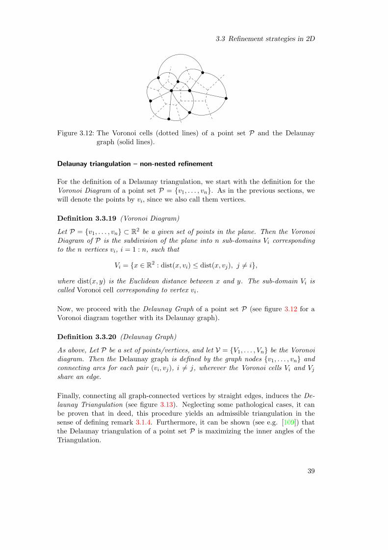
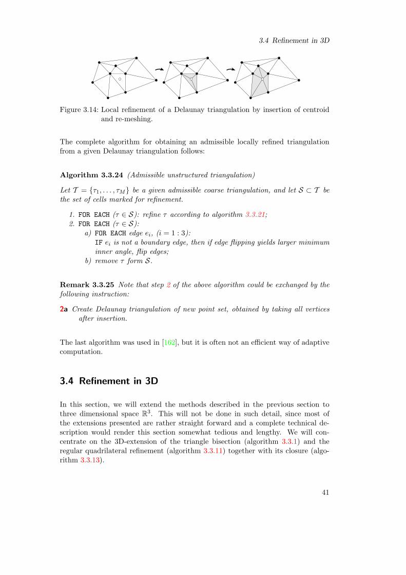
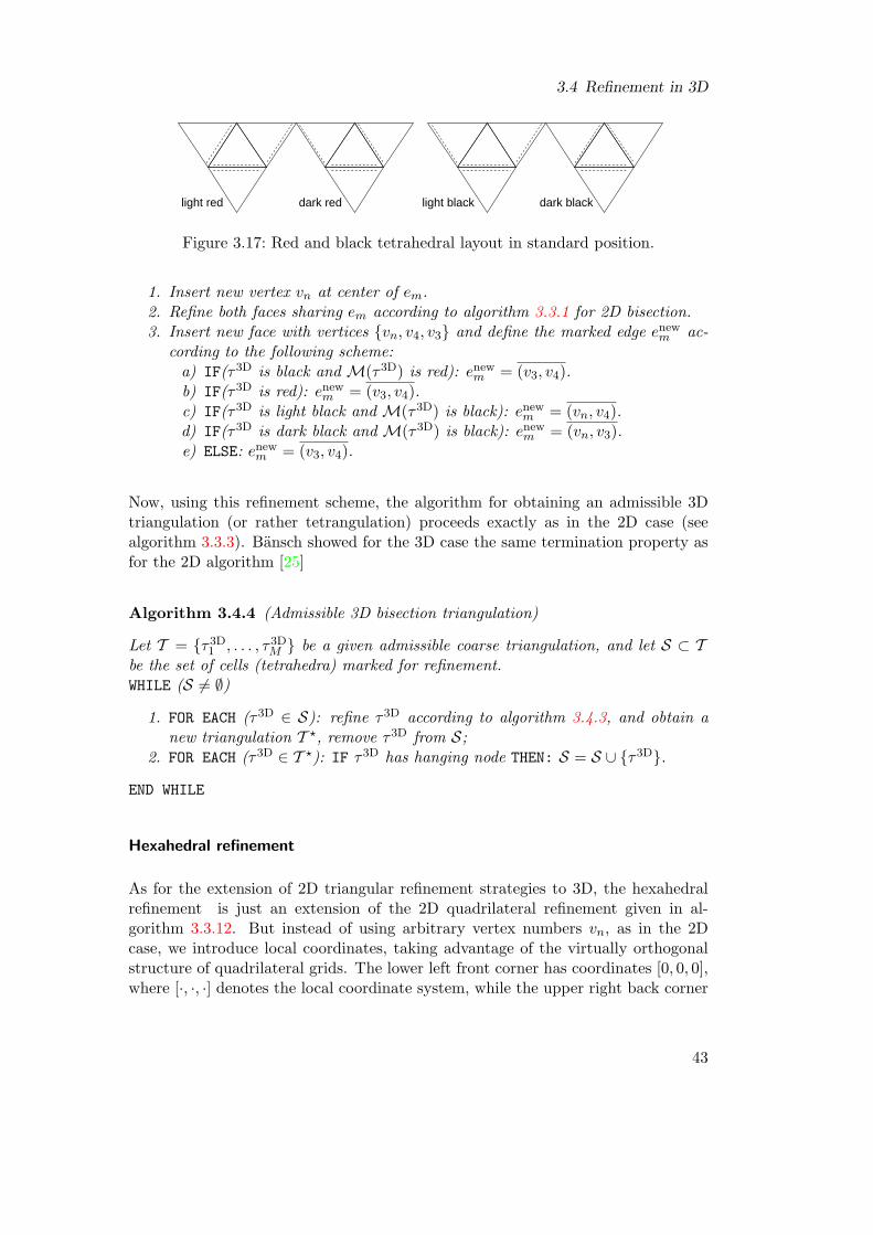
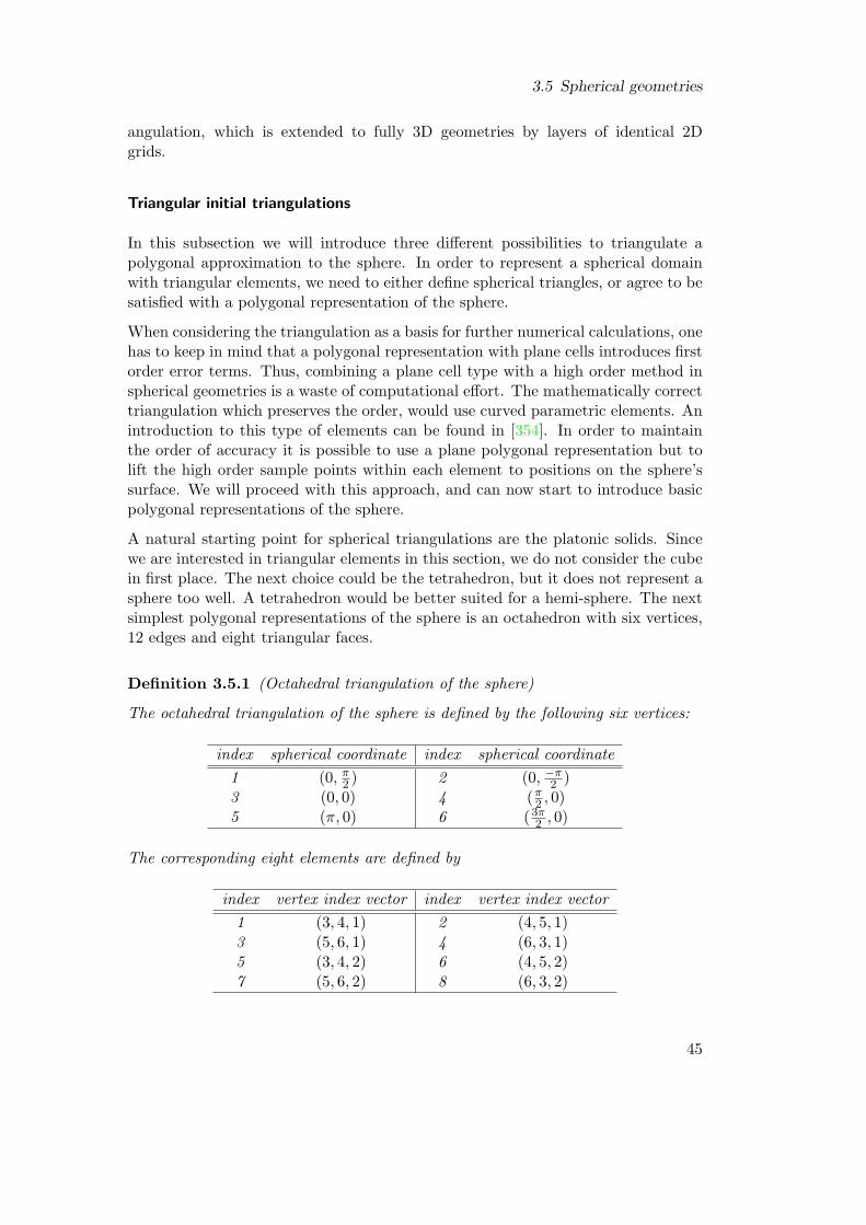
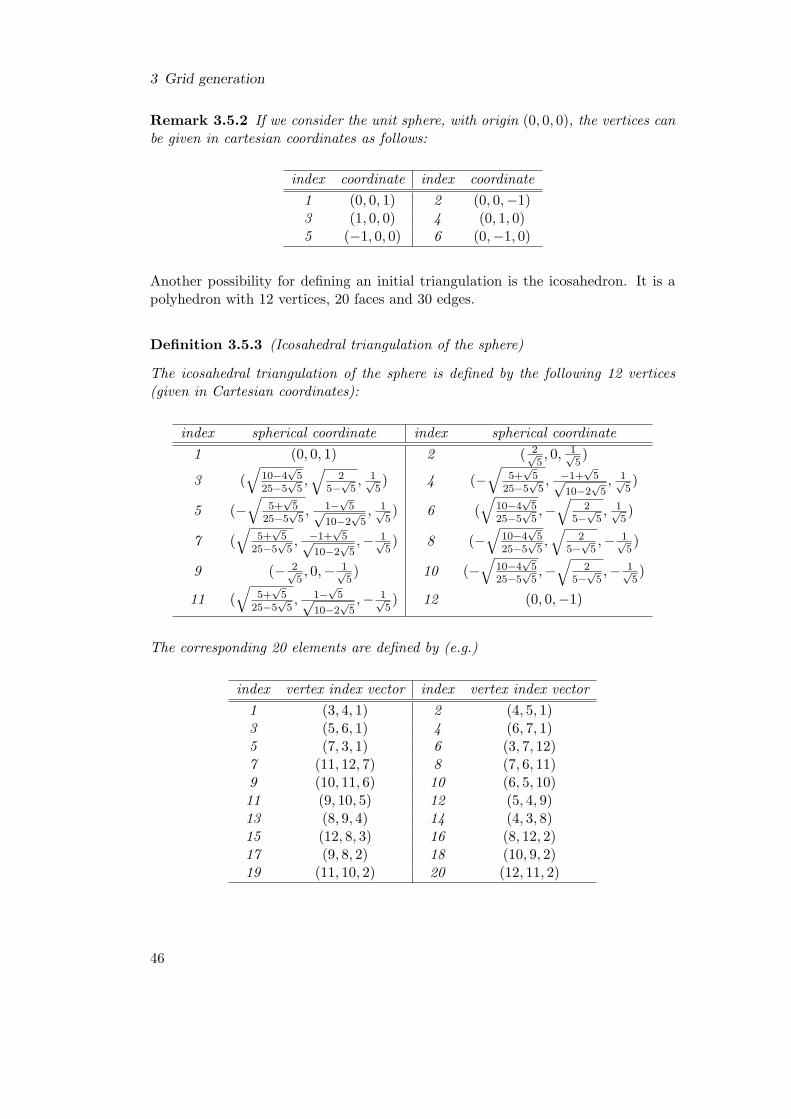
Two different tasks characterize the art of mesh generation: Automatic generationof a (coarse) mesh for a given – in most cases polygonal – domain; and efficientrefinement and un-refinement of a given initial mesh. Automatic mesh generation isstill an open field of research, since up to now, there is no fully automatic meshingtool available that can cover all demands. However, some very impressive resultshave been gained and the reader is referred to the literature for an overview [224, 283,385]. Since we are mostly concerned with spherical geometries without boundaries,we will focus on the second part, mesh refinement and un-refinement strategies,in this chapter. Section 3.5 reviews several initial grids for a special domain: thesphere.

3.1 Notation

In order to describe meshes formally correct, we need to introduce some notation.Let us begin with the basic definition of a triangulation. Note that by triangulationwe do not necessarily mean a triangular mesh. So let us define a cell first, were wewant to assume that cells in a triangulation are k-simplices..

Definition 3.1.1 (k-simplex)

Let P = P1, . . . , Pk ⊂ Rd be a (linearly independent) set of points (vertices) in thed-dimensional space. Then the convex hull of P is a k-simplex, where the convexhull is the intersection of all convex sets in Rd that contain P.

Example 3.1.2 (Simplicial cell types)

• A triangle is a 3-simplex in Rd.

25

3 Grid generation

• A hexahedral cell in R3 is a 8-simplex.• A tetrahedral cell in R3 is a 4-simplex.

Definition 3.1.3 (Triangulation)

Let G $ Rd be the finite d-dimensional and polygonal computational domain. ThenT = T (G) = τ1, . . . , τM, M number of cells, is an admissible triangulation, if

1. the cells τi, i = 1 : M , are open disjoint k-simplices in G, which cover thewhole domain:

τi ∩ τj = ∅ for i 6= j;⋃

i=1:M

τi = G.

2. for i 6= j is τi∩ τj either empty, or a common l-simplex with l < k (a commonedge, face, etc.).

Admissible triangulations are often called conforming triangulations.

Remark 3.1.4 When considering triangular cells in R2, definition 3.1.3 is equiv-alent to the definition given in many graph-based textbooks (see [109]): Let P =P1, . . . , Pn be a set of points in the plane (R2). A maximal planar subdivisionS is defined as a subdivision in which no edge can be added without destroying itsplanarity, i.e. any edge that is not in S intersects an edge in S. An admissibletriangulation is defined as a maximal planar subdivision with vertex set P.

Remark 3.1.5 Note that definition 3.1.3 is cell based. Therefore, when dealing withnode based methods, e.g. finite difference methods, only vertices of a triangulationare considered.

Remark 3.1.6 (Hanging node)

The above definition 3.1.3 defines an admissible triangulation, that is one withouthanging nodes. A hanging node is a node on an unrefined edge (see figure 3.1).Since many grid types incorporate hanging nodes we do not necessarily require ad-missible triangulations. A non-admissible triangulation is given by definition 3.1.3,omitting the second requirement. A non-admissible triangulation is often callednon-conforming.

In what follows, we will mostly omit the argument G for simplicity, since in mostcases it will be clear or irrelevant how specifically G is defined. In order to char-acterize a triangulation we need a measure for the quality and an expression forhierarchies of triangulations.

26

3.1 Notation

Figure 3.1: Two hanging nodes each in two different triangulations

Definition 3.1.7 (Hierarchies of triangulations)

Let T1 = τ1, . . . , τM and T2 = τ1, . . . , τK two triangulations. If T2 is createdfrom T1 by refinement, we write T1 ≺ T2.

Definition 3.1.8 (Mesh width, inner angle and regularity)

Let the following parameters be defined for a cell τ in a triangulation T .

he,τ : length of longest edge in τ,

hB,τ : radius of circum-circle of τ,hb,τ : radius of inner circle of τ.

We define the following parameters for characterizing the mesh size of T :

he = minτ∈The,τ,

hB = minτ∈ThB,τ,

hb = minτ∈Thb,τ.

Let furthermore ϑτ be the smallest angle in τ . The smallest inner angle of T isgiven by

ϑ = minτ∈Tϑτ

Finally, T is called regular, if 0 ϑ π.

Note that sincehb,τ < he,τ < hB,τ < Cϑhb,τ ,

where Cϑ is a constant that depends only on the smallest inner angle, all meshwidth parameters are equivalent to each other. Therefore, we often just use thenotation h for mesh width, without specifying which specific measure is to beused.

27

3 Grid generation

Remark 3.1.9 Since the sum of all inner angles of a triangle is π, for triangula-tions with triangular elements, the definition of regular in definition 3.1.8 impliesthat ϑ is close to π

3 . For quadrilateral triangulations a similar remark holds with ϑclose to π

2 .

Note that the regularity condition is equivalent to 0 hbhB

= C−1ϑ < 1.

3.2 Grid types

In this section different grid types are classified. A first attempt to classify gridtypes can be found for example in [87, 199]. These classifications have been de-veloped mainly for automatic mesh generation methods in engineering. However,since we are concerned with adaptively refined grids, we propose a distinct approachhere.

The first criterion of distinction between grids is the admissibility condition. Ad-missible (or conforming) grids do not allow hanging nodes. Both quadrilateral andtriangular grids can have hanging nodes, when refined locally, depending on therefinement strategy.

A second important distinction between grids is their orthogonality. Quadrilateralgrids have orthogonality properties, making them suitable for using 1D basis func-tions with tensor product expansion to d dimensions. When considering higherdimensional triangulations, also mixed grid types can occur, where the horizontalgrid is (non-orthogonal) triangular while the vertical dimension is discretized by anorthogonal quadrilateral extension, to give an example.

An important distinction is nesting. For locally refined meshes non-nested grids arecreated by defining new nodes and then completely re-meshing the triangulation.With nested grids, local refinement of single mesh elements with a certain refinementstrategy is performed. Nested meshes allow for (more or less) straight forwardimplementation of multi-grid methods.

A fourth category of distinction concerns structure, which we formally define.

Definition 3.2.1 (Structured and unstructured mesh)

A mesh is called structured, if the nodes can be ordered by an index array of ddimensions (i1, i2, . . . , id) and if neighboring nodes can be accessed by increasing theindex, e.g. (i1, i2 + 1, . . . , id). Otherwise a mesh is called unstructured.

Note that for an unstructured mesh additional data is required to define neigh-borhood relations (this is the so called connectivity). In adaptive grid generation,even logically structured meshes are sometimes treated like unstructured meshes,

28

3.2 Grid types

Table 3.1: Naming convention for adaptive grids

Position Tag Description1 C C: conforming2 O O: orthogonal3 N N: nested4 S S: structured5 T/H/P T: triangular/tetrahedral

H: quadrilateral/hexahedralP: polygonal/polyhedric

because then no different approaches have to be used in uniform (structured) andlocally refined (unstructured) areas.

For a short and precise descriptions of meshes we introduce a naming convention forgrid types given in table 3.1. The first four positions of the name-code correspondto the above classification, while the fifth position corresponds to a name for thegeometry of grid cells. In case a grid does not have one or the other of the tabulatedcharacteristic properties, the naming code is omitted. With this naming convention,a locally refined block-structured quadrilateral grid as used e.g. in [216] could becalled a ONSH-grid, while a bisected triangular grid like in amatos would be calledCNT-grid. A Delaunay triangulation is of type CT.

In order to further characterize a mesh, we can look at the number of refinementsas an indicator of resolution ratio. Most gridding schemes start with a given ini-tial mesh, which is uniformly refined up to a given level of refinement and thenfurther refined locally. For triangular meshes derived from an icosahedral initialdiscretization of the sphere, Baumgardner and Frederickson and more recently Gi-raldo have introduced a classification of uniform triangular refinements [163, 30].For a more universal convention and assuming that we have nested grids, we pro-pose a pair of numbers [c : f ] where c indicates the number of uniform refinements,i.e. c represents the coarsest mesh level used in computations, and f is the finestgrid level.

Extending the above naming convetion with this pair, we have a ONSH[3 : 6]-grid in [216], while in [39] the finest mesh is of type CNT[4 : 19]. If we haveuniform grids, then we can omit one of the entries, obtaining CNT[15] ≡ CNT[15 :15].

If refinement levels are inadequate or not available for the classification, we couldconsider resolutions of the coarsest grid cells and the finest grid cells. Thus, CNT[4 :19] ≡ CNT(230 : 5)[km]. For distinction, we have put the resolution in bracketsinstead of square brackets and added a subscript denoting the unit (Kilometers

29

3 Grid generation

here). As another example, the operational global model (GME) of the GermanWeather Service (DWD) has type CSH(40)[km].

3.3 Refinement strategies in 2D

In this section we give an overview of commonly used refinement strategies. Whenselecting a refinement strategy, it is important to have in mind the objectives ofthe refinement strategy. One could either optimize grid quality, but has to dealwith algorithmic complexity. On the other hand, it could be important to maintainorthogonality, but then admissibility cannot be maintained. There is no singlestrategy that optimizes all of the existing desirable properties of a mesh. For agood overview of mesh generation especially in engineering applications, see [385].A comparison of refinement strategies in the context of finite element methods isgiven in [284].

Triangular bisection

A very simple, yet powerful refinement strategy for triangular meshes is the bisectionstrategy. It constructs two daughter triangles from one mother. In order to maintainregularity of the mesh, only marked edges are allowed to be refined. Defined in aniterative procedure, this strategy leads to locally adaptive, nested, and admissiblemeshes.

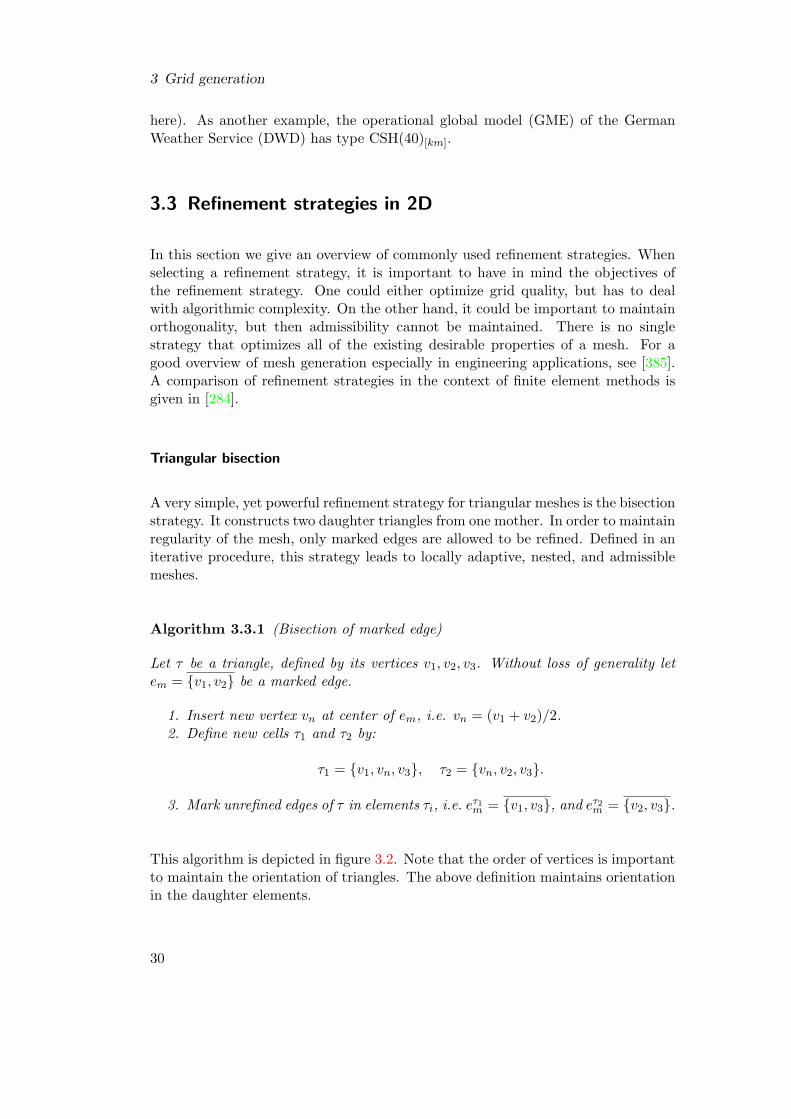
Algorithm 3.3.1 (Bisection of marked edge)

Let τ be a triangle, defined by its vertices v1, v2, v3. Without loss of generality letem = v1, v2 be a marked edge.

1. Insert new vertex vn at center of em, i.e. vn = (v1 + v2)/2.2. Define new cells τ1 and τ2 by:

τ1 = v1, vn, v3, τ2 = vn, v2, v3.

3. Mark unrefined edges of τ in elements τi, i.e. eτ1m = v1, v3, and eτ2m = v2, v3.

This algorithm is depicted in figure 3.2. Note that the order of vertices is importantto maintain the orientation of triangles. The above definition maintains orientationin the daughter elements.

30


marked edge

Figure 3.2: Bisection of marked edge algorithm 3.3.1 acting on a triangle.

Figure 3.3: The iterative process to construct a triangulation by algorithm 3.3.3.The shaded area corresponds to the set S, dotted lines depict markededges, and a hanging node is marked by an open circle.

Remark 3.3.2 (Bisection of longest edge)

There is a variant of algorithm 3.3.1, called bisection of longest edge. It differs fromthe above given algorithm in that it refines the longest edge only. When startingwith a sufficiently regular initial triangle, both algorithms are equivalent. However,marking an edge with the above scheme results in less computational effort, becauselongest edge bisection needs to evaluate the edge length for each of the three edgesin each step.

In order to create a complete mesh with regions of local refinement we have to usethe bisection algorithm iteratively:

Algorithm 3.3.3 (Admissible bisection triangulation)

Let T = τ1, . . . , τM be a given admissible coarse triangulation, and let S ⊂ T bethe set of cells marked for refinement.WHILE (S 6= ∅)

1. FOR EACH (τ ∈ S): refine τ according to algorithm 3.3.1, and obtain a newtriangulation T ?, remove τ from S (S is empty at the end of this step);

2. FOR EACH (τ ∈ T ?): IF τ has hanging node THEN: S = S ∪ τ.

END WHILE

Algorithm 3.3.3 is visualized in figure 3.3. It can be shown that algorithm 3.3.3converges, i.e. S is in fact empty after a finite number of iterations. Furthermore, it

31

3 Grid generation

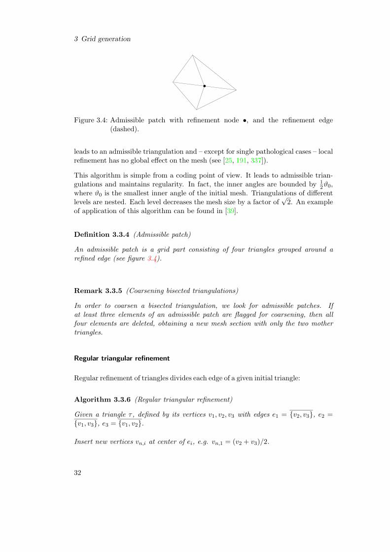
Figure 3.4: Admissible patch with refinement node •, and the refinement edge(dashed).

leads to an admissible triangulation and – except for single pathological cases – localrefinement has no global effect on the mesh (see [25, 191, 337]).

This algorithm is simple from a coding point of view. It leads to admissible trian-gulations and maintains regularity. In fact, the inner angles are bounded by 1

2ϑ0,where ϑ0 is the smallest inner angle of the initial mesh. Triangulations of differentlevels are nested. Each level decreases the mesh size by a factor of

√2. An example

of application of this algorithm can be found in [39].

Definition 3.3.4 (Admissible patch)

An admissible patch is a grid part consisting of four triangles grouped around arefined edge (see figure 3.4).

Remark 3.3.5 (Coarsening bisected triangulations)

In order to coarsen a bisected triangulation, we look for admissible patches. Ifat least three elements of an admissible patch are flagged for coarsening, then allfour elements are deleted, obtaining a new mesh section with only the two mothertriangles.

Regular triangular refinement

Regular refinement of triangles divides each edge of a given initial triangle:

Algorithm 3.3.6 (Regular triangular refinement)

Given a triangle τ , defined by its vertices v1, v2, v3 with edges e1 = v2, v3, e2 =v1, v3, e3 = v1, v2.

Insert new vertices vn,i at center of ei, e.g. vn,1 = (v2 + v3)/2.

32


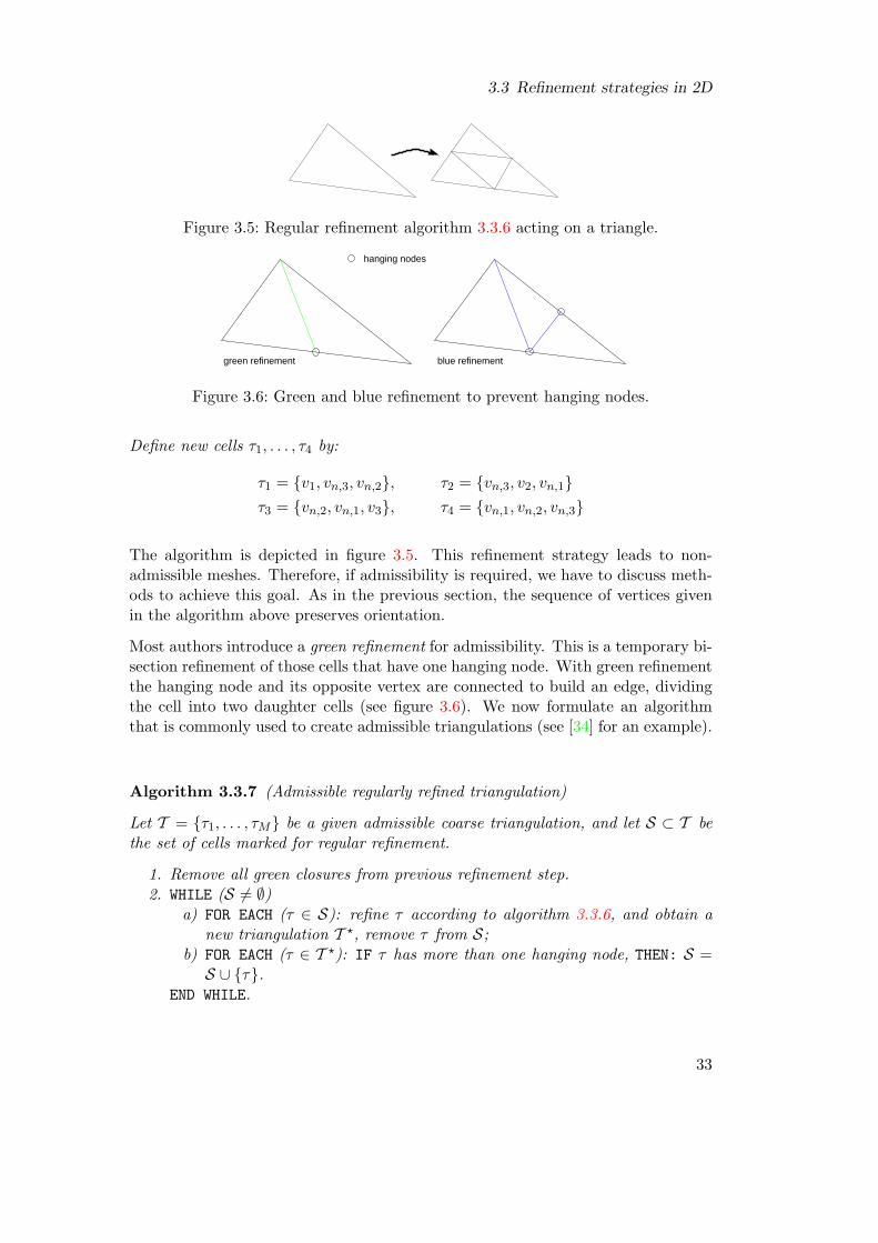
Figure 3.5: Regular refinement algorithm 3.3.6 acting on a triangle.

blue refinement

hanging nodes

green refinement

Figure 3.6: Green and blue refinement to prevent hanging nodes.

Define new cells τ1, . . . , τ4 by:

τ1 = v1, vn,3, vn,2, τ2 = vn,3, v2, vn,1τ3 = vn,2, vn,1, v3, τ4 = vn,1, vn,2, vn,3

The algorithm is depicted in figure 3.5. This refinement strategy leads to non-admissible meshes. Therefore, if admissibility is required, we have to discuss meth-ods to achieve this goal. As in the previous section, the sequence of vertices givenin the algorithm above preserves orientation.

Most authors introduce a green refinement for admissibility. This is a temporary bi-section refinement of those cells that have one hanging node. With green refinementthe hanging node and its opposite vertex are connected to build an edge, dividingthe cell into two daughter cells (see figure 3.6). We now formulate an algorithmthat is commonly used to create admissible triangulations (see [34] for an example).

Algorithm 3.3.7 (Admissible regularly refined triangulation)

Let T = τ1, . . . , τM be a given admissible coarse triangulation, and let S ⊂ T bethe set of cells marked for regular refinement.

1. Remove all green closures from previous refinement step.2. WHILE (S 6= ∅)

a) FOR EACH (τ ∈ S): refine τ according to algorithm 3.3.6, and obtain anew triangulation T ?, remove τ from S;

b) FOR EACH (τ ∈ T ?): IF τ has more than one hanging node, THEN: S =S ∪ τ.

END WHILE.

33

3 Grid generation

3. FOR EACH (τ ∈ T ?): IF τ has hanging node, THEN: refine τ by green refine-ment.

Remark 3.3.8 As in subsection 3.3, it can be shown that algorithm 3.3.7 leads toan admissible triangulation. The inner angles are bounded, since regular refinementcreates four similar daughter triangles form each mother triangle.

Remark 3.3.9 Some authors introduce a blue refinement to treat cells with twohanging nodes. In order to obtain a blue refinement, proceed as follows (see figure3.6):

1. bisect the cell by taking the hanging node on the longer edge and its oppositevertex as bisection edge;

2. bisect the daughter element of step 1, which contains the remaining hangingnode by connecting this hanging node with the first hanging node.

Remark 3.3.10 (Coarsening regularly refined triangulation)

Since green or blue refinements are removed from the grid before refinement/coarsening,we only have to consider regularly refined elements for coarsening. So, in order tocoarsen a regularly refined triangular element, the four daughter elements are re-moved, leaving the mother on the now finest mesh level. Coarsening is performed ifthree or more daughters are flagged for coarsening.

Quadrilateral refinement

Quadrilateral grids are very popular since several advantages can be exploited forefficient numerical calculations. Quadrilaterals are well suited for efficient interpo-lation/quadrature schemes, because the local coordinate system can be formulatedorthogonally. A structured data layout can be achieved easily. And the ratio ofcell number to node number (which is a measure for computational efficiency) issmaller than in triangular meshes. On the other hand, admissibility is often hurt.And more importantly, complex geometries are not easily represented by quadri-laterals. As a simplification and requirement for orthogonality, we want to assumeconvex quadrilaterals throughout this section.

The most simple refinement strategy, is to insert one vertex and add edges to thecenters of all cell edges:

Algorithm 3.3.11 (General quadrilateral refinement)

Given a Quad χ, defined by its vertices v1, . . . , v4 with edges e1 = v1, v2, . . . ,e4 = v4, v1.

34


a

b

Figure 3.7: Algorithm 3.3.11 for general quadrilateral refinement (a) and 3.3.12 forregular quadrilateral refinement acting on a cell.

1. Insert new vertex vn inside χ.2. Create new edge vertices vn,1, . . . , vn,4 by

vn,1 =(v1 + v2)

2, . . . , vn,4 =

(v4 + v1)2

.

3. Define new cells χ1, . . . , χ4 by:

χ1 = v1, vn,1, vn, vn,4, χ2 = vn,1, v2, vn,2, vnχ3 = vn, vn,2, v3, vn,3, χ4 = vn,4, vn, vn,3, v4

Remark 3.3.12 (Regular quadrilateral refinement)

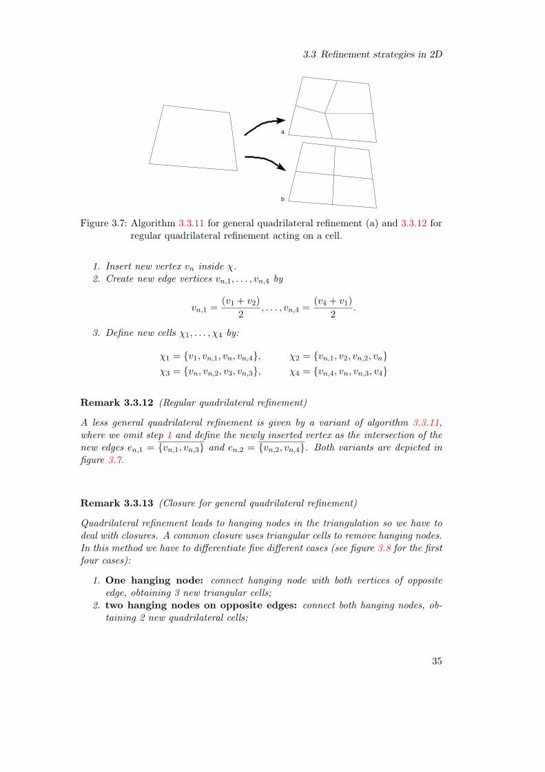
A less general quadrilateral refinement is given by a variant of algorithm 3.3.11,where we omit step 1 and define the newly inserted vertex as the intersection of thenew edges en,1 = vn,1, vn,3 and en,2 = vn,2, vn,4. Both variants are depicted infigure 3.7.

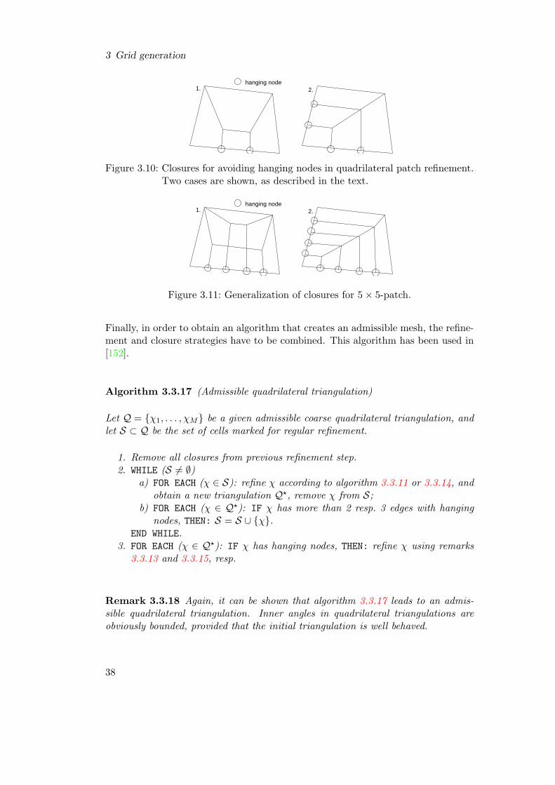
Remark 3.3.13 (Closure for general quadrilateral refinement)

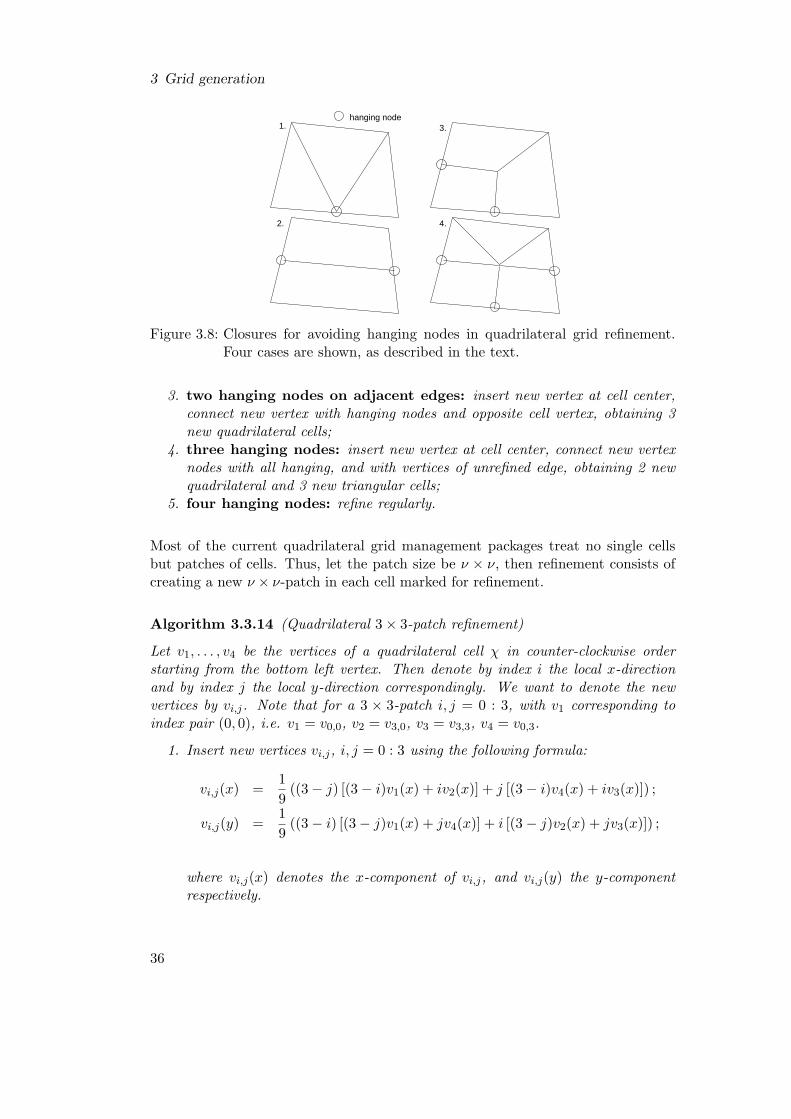
Quadrilateral refinement leads to hanging nodes in the triangulation so we have todeal with closures. A common closure uses triangular cells to remove hanging nodes.In this method we have to differentiate five different cases (see figure 3.8 for the firstfour cases):

1. One hanging node: connect hanging node with both vertices of oppositeedge, obtaining 3 new triangular cells;

2. two hanging nodes on opposite edges: connect both hanging nodes, ob-taining 2 new quadrilateral cells;

35

3 Grid generation

hanging node1.

2.

3.

4.

Figure 3.8: Closures for avoiding hanging nodes in quadrilateral grid refinement.Four cases are shown, as described in the text.

3. two hanging nodes on adjacent edges: insert new vertex at cell center,connect new vertex with hanging nodes and opposite cell vertex, obtaining 3new quadrilateral cells;

4. three hanging nodes: insert new vertex at cell center, connect new vertexnodes with all hanging, and with vertices of unrefined edge, obtaining 2 newquadrilateral and 3 new triangular cells;

5. four hanging nodes: refine regularly.

Most of the current quadrilateral grid management packages treat no single cellsbut patches of cells. Thus, let the patch size be ν × ν, then refinement consists ofcreating a new ν × ν-patch in each cell marked for refinement.

Algorithm 3.3.14 (Quadrilateral 3× 3-patch refinement)

Let v1, . . . , v4 be the vertices of a quadrilateral cell χ in counter-clockwise orderstarting from the bottom left vertex. Then denote by index i the local x-directionand by index j the local y-direction correspondingly. We want to denote the newvertices by vi,j. Note that for a 3 × 3-patch i, j = 0 : 3, with v1 corresponding toindex pair (0, 0), i.e. v1 = v0,0, v2 = v3,0, v3 = v3,3, v4 = v0,3.

1. Insert new vertices vi,j, i, j = 0 : 3 using the following formula:

vi,j(x) =19

((3− j) [(3− i)v1(x) + iv2(x)] + j [(3− i)v4(x) + iv3(x)]) ;

vi,j(y) =19

((3− i) [(3− j)v1(x) + jv4(x)] + i [(3− j)v2(x) + jv3(x)]) ;

where vi,j(x) denotes the x-component of vi,j, and vi,j(y) the y-componentrespectively.

36


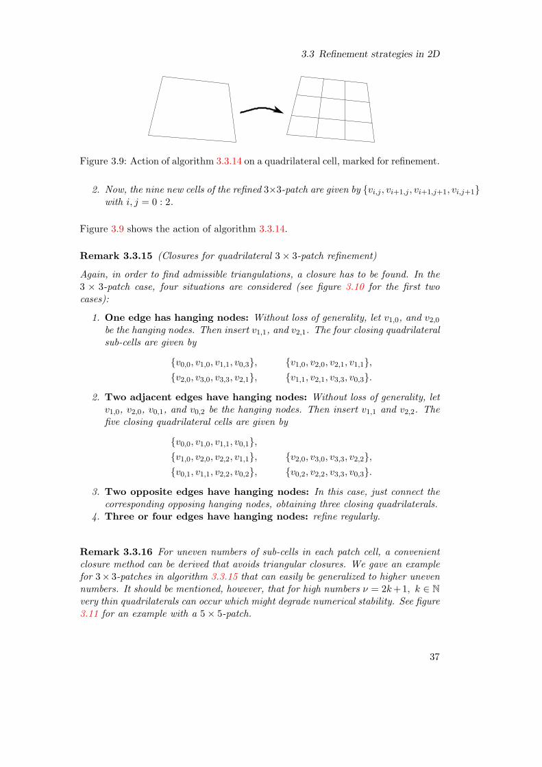
Figure 3.9: Action of algorithm 3.3.14 on a quadrilateral cell, marked for refinement.

2. Now, the nine new cells of the refined 3×3-patch are given by vi,j , vi+1,j , vi+1,j+1, vi,j+1with i, j = 0 : 2.

Figure 3.9 shows the action of algorithm 3.3.14.

Remark 3.3.15 (Closures for quadrilateral 3× 3-patch refinement)

Again, in order to find admissible triangulations, a closure has to be found. In the3 × 3-patch case, four situations are considered (see figure 3.10 for the first twocases):

1. One edge has hanging nodes: Without loss of generality, let v1,0, and v2,0be the hanging nodes. Then insert v1,1, and v2,1. The four closing quadrilateralsub-cells are given by

v0,0, v1,0, v1,1, v0,3, v1,0, v2,0, v2,1, v1,1,v2,0, v3,0, v3,3, v2,1, v1,1, v2,1, v3,3, v0,3.

2. Two adjacent edges have hanging nodes: Without loss of generality, letv1,0, v2,0, v0,1, and v0,2 be the hanging nodes. Then insert v1,1 and v2,2. Thefive closing quadrilateral cells are given by

v0,0, v1,0, v1,1, v0,1,v1,0, v2,0, v2,2, v1,1, v2,0, v3,0, v3,3, v2,2,v0,1, v1,1, v2,2, v0,2, v0,2, v2,2, v3,3, v0,3.

3. Two opposite edges have hanging nodes: In this case, just connect thecorresponding opposing hanging nodes, obtaining three closing quadrilaterals.

4. Three or four edges have hanging nodes: refine regularly.

Remark 3.3.16 For uneven numbers of sub-cells in each patch cell, a convenientclosure method can be derived that avoids triangular closures. We gave an examplefor 3× 3-patches in algorithm 3.3.15 that can easily be generalized to higher unevennumbers. It should be mentioned, however, that for high numbers ν = 2k+1, k ∈ Nvery thin quadrilaterals can occur which might degrade numerical stability. See figure3.11 for an example with a 5× 5-patch.

37

3 Grid generation

hanging node1. 2.

Figure 3.10: Closures for avoiding hanging nodes in quadrilateral patch refinement.Two cases are shown, as described in the text.

hanging node1. 2.

Figure 3.11: Generalization of closures for 5× 5-patch.

Finally, in order to obtain an algorithm that creates an admissible mesh, the refine-ment and closure strategies have to be combined. This algorithm has been used in[152].

Algorithm 3.3.17 (Admissible quadrilateral triangulation)

Let Q = χ1, . . . , χM be a given admissible coarse quadrilateral triangulation, andlet S ⊂ Q be the set of cells marked for regular refinement.

1. Remove all closures from previous refinement step.2. WHILE (S 6= ∅)

a) FOR EACH (χ ∈ S): refine χ according to algorithm 3.3.11 or 3.3.14, andobtain a new triangulation Q?, remove χ from S;

b) FOR EACH (χ ∈ Q?): IF χ has more than 2 resp. 3 edges with hangingnodes, THEN: S = S ∪ χ.

END WHILE.3. FOR EACH (χ ∈ Q?): IF χ has hanging nodes, THEN: refine χ using remarks

3.3.13 and 3.3.15, resp.

Remark 3.3.18 Again, it can be shown that algorithm 3.3.17 leads to an admis-sible quadrilateral triangulation. Inner angles in quadrilateral triangulations areobviously bounded, provided that the initial triangulation is well behaved.

38


Figure 3.12: The Voronoi cells (dotted lines) of a point set P and the Delaunaygraph (solid lines).

Delaunay triangulation – non-nested refinement

For the definition of a Delaunay triangulation, we start with the definition for theVoronoi Diagram of a point set P = v1, . . . , vn. As in the previous sections, wewill denote the points by vi, since we also call them vertices.

Definition 3.3.19 (Voronoi Diagram)

Let P = v1, . . . , vn ⊂ R2 be a given set of points in the plane. Then the VoronoiDiagram of P is the subdivision of the plane into n sub-domains Vi correspondingto the n vertices vi, i = 1 : n, such that

Vi = x ∈ R2 : dist(x, vi) ≤ dist(x, vj), j 6= i,

where dist(x, y) is the Euclidean distance between x and y. The sub-domain Vi iscalled Voronoi cell corresponding to vertex vi.

Now, we proceed with the Delaunay Graph of a point set P (see figure 3.12 for aVoronoi diagram together with its Delaunay graph).

Definition 3.3.20 (Delaunay Graph)

As above, Let P be a set of points/vertices, and let V = V1, . . . , Vn be the Voronoidiagram. Then the Delaunay graph is defined by the graph nodes v1, . . . , vn andconnecting arcs for each pair (vi, vj), i 6= j, wherever the Voronoi cells Vi and Vjshare an edge.

Finally, connecting all graph-connected vertices by straight edges, induces the De-launay Triangulation (see figure 3.13). Neglecting some pathological cases, it canbe proven that in deed, this procedure yields an admissible triangulation in thesense of defining remark 3.1.4. Furthermore, it can be shown (see e.g. [109]) thatthe Delaunay triangulation of a point set P is maximizing the inner angles of theTriangulation.

39

3 Grid generation

Figure 3.13: The Delaunay triangulation (solid lines) of a given point set togetherwith the Voronoi diagram (dotted lines).

The Delaunay triangulation of a point set P can be computed in O(n log n) op-erations with O(n) required storage positions, where n is the number of verticesin P. A practical algorithm (also for 3D Delaunay trianglulations) is given in[378].

In order to construct an adaptive method using a Delaunay triangulation, we needto specify a vertex insertion method. Again, we assume that there is a given initialtriangulation with a set of triangles marked for refinement. In principle, one couldtake a random distribution of points as an initial triangulation.

Algorithm 3.3.21 (Unstructured Vertex insertion)

Given a triangle τ , defined by its vertices v1, v2, v3.

Insert a new vertex vn at the barycenter of τ : vn = (v1 + v2 + v3)/3.

Define new cells τ1, . . . , τ3 by:

τ1 = v1, vn, v2, τ2 = v2, vn, v3, τ3 = v3, vn, v1

This algorithm is used in [20]. The insertion of new cells is depicted in figure3.14.

Remark 3.3.22 Note that algorithm 3.3.21 does not prevent inner angles to col-lapse. Therefore, in the algorithm for creating an complete triangulation, a re-meshing step is required (see algorithm 3.3.24, resp. remark 3.3.25).

Remark 3.3.23 Another vertex-based possibility to find locations for new nodes hasbeen used in [41]. Here, vertices are flagged for refinement instead of cells. Then,each corner of the corresponding Voronoi-cell is inserted as new vertex. After inser-tion of new nodes, re-meshing has to be performed. This method is especially suitedfor mesh-free methods, where only point locations are considered for calculations.

40

3.4 Refinement in 3D

Figure 3.14: Local refinement of a Delaunay triangulation by insertion of centroidand re-meshing.

The complete algorithm for obtaining an admissible locally refined triangulationfrom a given Delaunay triangulation follows:

Algorithm 3.3.24 (Admissible unstructured triangulation)

Let T = τ1, . . . , τM be a given admissible coarse triangulation, and let S ⊂ T bethe set of cells marked for refinement.

1. FOR EACH (τ ∈ S): refine τ according to algorithm 3.3.21;2. FOR EACH (τ ∈ S):

a) FOR EACH edge ei, (i = 1 : 3):IF ei is not a boundary edge, then if edge flipping yields larger minimuminner angle, flip edges;

b) remove τ form S.

Remark 3.3.25 Note that step 2 of the above algorithm could be exchanged by thefollowing instruction:

2a Create Delaunay triangulation of new point set, obtained by taking all verticesafter insertion.

The last algorithm was used in [162], but it is often not an efficient way of adaptivecomputation.


In this section, we will extend the methods described in the previous section tothree dimensional space R3. This will not be done in such detail, since most ofthe extensions presented are rather straight forward and a complete technical de-scription would render this section somewhat tedious and lengthy. We will con-centrate on the 3D-extension of the triangle bisection (algorithm 3.3.1) and theregular quadrilateral refinement (algorithm 3.3.11) together with its closure (algo-rithm 3.3.13).

41

3 Grid generation

v

4v3v 4v

2v

4v

1

Figure 3.15: Unfolding a tetrahedron into standard position, and notations for localvertex ordering and globally marked edge (dotted line).

*common face

? ***

Figure 3.16: Bisection of a tetrahedron (action of algorithm 3.4.3).

Tetrahedral bisection

In this section we follow an approach introduced by Bansch [25]. We start withdefining a tetrahedron with marked edges.

Definition 3.4.1 (Tetrahedron with globally marked edge)

Let τ3D be a tetrahedron, defined by its four vertices v1, . . . , v4 ⊂ R3, with facesτ1 = (v1, v2, v3), τ2 = (v2, v4, v3), τ3 = (v1, v3, v4), and τ4 = (v1, v4, v2) (see figure3.15. Let each of the τi have one marked edge such that exactly two of the faces sharetheir marked edge. We will call this edge a globally marked edge (of tetrahedronτ3D).

Remark 3.4.2 Note that the representation in figure 3.15 is called standard posi-tion. After rotation and scaling, this representation is unique, assuming that thereis only one globally marked edge (v1, v2).

When refining a tetrahedron, we can simply apply the 2D algorithms for refin-ing triangles to the faces. However, we have to define, how to set the markededge in the newly created face separating the two new tetrahedra (see figure 3.16).Bansch [25] uses the notion of red and black tetrahedra as given in figure 3.17.

Algorithm 3.4.3 (Tetrahedral Bisection)

Given a tetrahedron τ3D in standard position as defined in definition 3.4.1, with aglobally marked edge em = (v1, v2). We will denote the mother of τ3D by M(τ3D).

42


dark blacklight red dark red light black

Figure 3.17: Red and black tetrahedral layout in standard position.

1. Insert new vertex vn at center of em.2. Refine both faces sharing em according to algorithm 3.3.1 for 2D bisection.3. Insert new face with vertices vn, v4, v3 and define the marked edge enew

m ac-cording to the following scheme:

a) IF(τ3D is black and M(τ3D) is red): enewm = (v3, v4).

b) IF(τ3D is red): enewm = (v3, v4).

c) IF(τ3D is light black and M(τ3D) is black): enewm = (vn, v4).

d) IF(τ3D is dark black and M(τ3D) is black): enewm = (vn, v3).

e) ELSE: enewm = (v3, v4).

Now, using this refinement scheme, the algorithm for obtaining an admissible 3Dtriangulation (or rather tetrangulation) proceeds exactly as in the 2D case (seealgorithm 3.3.3). Bansch showed for the 3D case the same termination property asfor the 2D algorithm [25]

Algorithm 3.4.4 (Admissible 3D bisection triangulation)

Let T = τ3D1 , . . . , τ3D

M be a given admissible coarse triangulation, and let S ⊂ Tbe the set of cells (tetrahedra) marked for refinement.WHILE (S 6= ∅)

1. FOR EACH (τ3D ∈ S): refine τ3D according to algorithm 3.4.3, and obtain anew triangulation T ?, remove τ3D from S;

2. FOR EACH (τ3D ∈ T ?): IF τ3D has hanging node THEN: S = S ∪ τ3D.

END WHILE

Hexahedral refinement

As for the extension of 2D triangular refinement strategies to 3D, the hexahedralrefinement is just an extension of the 2D quadrilateral refinement given in al-gorithm 3.3.12. But instead of using arbitrary vertex numbers vn, as in the 2Dcase, we introduce local coordinates, taking advantage of the virtually orthogonalstructure of quadrilateral grids. The lower left front corner has coordinates [0, 0, 0],where [·, ·, ·] denotes the local coordinate system, while the upper right back corner

43

3 Grid generation

[0,0,1][1,1,1]

[0,0,0][0,0,0]

[2,2,2]

[1,1,1]

[1,0,0]

[0,1,0]

Figure 3.18: Hexahedral refinement, the action of algorithm 3.4.5.

has coordinates [1, 1, 1] or [2, 2, 2] after re-normalization and refinement (see figure3.18).

Algorithm 3.4.5 (Regular hexahedral refinement)

Given a hexahedron τ3D, defined by its vertices v1 = [0, 0, 0], . . . , v8 = [1, 1, 1], withfaces ν1, . . . , ν6.

1. Refine each face νi (i = 1 : 6), using algorithm 3.3.12.2. Connect opposite center vertices. The intersection of these edges yields an-

other new vertex vn.3. Define new cells τ3D

0,0,0, . . . , τ3D1,1,1 by:

τ3Di,j,k = [0, 0, 0], [1, 0, 0], [1, 1, 0], [0, 1, 0] ,

[0, 0, 1], [1, 0, 1], [1, 1, 1], [0, 1, 1] + [i, j, k], i, j, k = 0, 1.

As in the 2D case, hexahedral refinement causes non-admissible triangulations, i.e.hanging nodes. Therefore, a closure mechanism has to be defined, if admissible tri-angulations are required. For an extension of the 2D algorithm, pyramidal elementscan be introduced. However, the number of cases that have to be tackled and the re-gion of influence for closures is by far not as simple as in the 2D case. In fact, it is notpossible to define a point insertion algorithm that results in a conforming (purely)hexahedral mesh in complete generality (see chapter 21 in [385] by R. Schneiders).So we will omit the discussion of all those cases here.

Most applications with hexahedral mesh refinement use solution techniques thatcan handle hanging nodes. Thus, a non-conforming block-wise refinement strategyfor local refinement is often applied (see for example [202]).

3.5 Spherical geometries

In order to find discrete representations of the sphere, we have to start with aninitial triangulation T . In most cases, the sphere is triangulated by a 2D tri-

44


angulation, which is extended to fully 3D geometries by layers of identical 2Dgrids.

Triangular initial triangulations

In this subsection we will introduce three different possibilities to triangulate apolygonal approximation to the sphere. In order to represent a spherical domainwith triangular elements, we need to either define spherical triangles, or agree to besatisfied with a polygonal representation of the sphere.

When considering the triangulation as a basis for further numerical calculations, onehas to keep in mind that a polygonal representation with plane cells introduces firstorder error terms. Thus, combining a plane cell type with a high order method inspherical geometries is a waste of computational effort. The mathematically correcttriangulation which preserves the order, would use curved parametric elements. Anintroduction to this type of elements can be found in [354]. In order to maintainthe order of accuracy it is possible to use a plane polygonal representation but tolift the high order sample points within each element to positions on the sphere’ssurface. We will proceed with this approach, and can now start to introduce basicpolygonal representations of the sphere.

A natural starting point for spherical triangulations are the platonic solids. Sincewe are interested in triangular elements in this section, we do not consider the cubein first place. The next choice could be the tetrahedron, but it does not represent asphere too well. A tetrahedron would be better suited for a hemi-sphere. The nextsimplest polygonal representations of the sphere is an octahedron with six vertices,12 edges and eight triangular faces.

Definition 3.5.1 (Octahedral triangulation of the sphere)

The octahedral triangulation of the sphere is defined by the following six vertices:

index spherical coordinate index spherical coordinate1 (0, π2 ) 2 (0, −π2 )3 (0, 0) 4 (π2 , 0)5 (π, 0) 6 (3π

2 , 0)

The corresponding eight elements are defined by

index vertex index vector index vertex index vector1 (3, 4, 1) 2 (4, 5, 1)3 (5, 6, 1) 4 (6, 3, 1)5 (3, 4, 2) 6 (4, 5, 2)7 (5, 6, 2) 8 (6, 3, 2)

45

3 Grid generation

Remark 3.5.2 If we consider the unit sphere, with origin (0, 0, 0), the vertices canbe given in cartesian coordinates as follows:

index coordinate index coordinate1 (0, 0, 1) 2 (0, 0,−1)3 (1, 0, 0) 4 (0, 1, 0)5 (−1, 0, 0) 6 (0,−1, 0)

Another possibility for defining an initial triangulation is the icosahedron. It is apolyhedron with 12 vertices, 20 faces and 30 edges.

Definition 3.5.3 (Icosahedral triangulation of the sphere)

The icosahedral triangulation of the sphere is defined by the following 12 vertices(given in Cartesian coordinates):

index spherical coordinate index spherical coordinate1 (0, 0, 1) 2 ( 2√

5, 0, 1√

5)

3 (√

10−4√

525−5

√5,√

25−

√5, 1√

5) 4 (−

√5+

√5

25−5√

5, −1+

√5√

10−2√

5, 1√

5)

5 (−√

5+√

525−5

√5, 1−

√5√

10−2√

5, 1√

5) 6 (

√10−4

√5

25−5√

5,−√

25−

√5, 1√

5)

7 (√

5+√

525−5

√5, −1+

√5√

10−2√

5,− 1√

5) 8 (−

√10−4

√5

25−5√

5,√

25−

√5,− 1√

5)

9 (− 2√5, 0,− 1√

5) 10 (−

√10−4

√5

25−5√

5,−√

25−

√5,− 1√

5)

11 (√

5+√

525−5

√5, 1−

√5√

10−2√

5,− 1√

5) 12 (0, 0,−1)

The corresponding 20 elements are defined by (e.g.)

index vertex index vector index vertex index vector1 (3, 4, 1) 2 (4, 5, 1)3 (5, 6, 1) 4 (6, 7, 1)5 (7, 3, 1) 6 (3, 7, 12)7 (11, 12, 7) 8 (7, 6, 11)9 (10, 11, 6) 10 (6, 5, 10)11 (9, 10, 5) 12 (5, 4, 9)13 (8, 9, 4) 14 (4, 3, 8)15 (12, 8, 3) 16 (8, 12, 2)17 (9, 8, 2) 18 (10, 9, 2)19 (11, 10, 2) 20 (12, 11, 2)

46


Figure 3.19: Octahedral triangulation of sphere: initial triangulation (left, with 8triangles) and after uniform refinement (right, with 1024 triangles).

Figure 3.20: Icosahedral triangulation of sphere: initial triangulation (left, with 20triangles) and after refinement (right, with 1280 triangles).

Figure 3.21: Truncated icosahedral triangulation of sphere (buckyball): initial trian-gulation (left, with 180 triangles) and after uniform refinement (right,with 1440 triangles).

47

3 Grid generation

Remark 3.5.4 The rather obscure coordinate values in definition 3.5.3 can be cir-cumvented, when considering a sphere with radius r = 1

2

√5. Then, the coordinates

can be given in 3D cartesian form by

index i x-coordinate y-coordinate z-coordinate1 0.0 0.0 r2 0.0 0.0 −r

3:7 cos(

2(i−3)π5

)sin(

2(i−3)π5

)0.5

8:12 cos(π+2(i−8)π

5

)sin(π+2(i−8)π

5

)−0.5

Remark 3.5.5 In spherical coordinates(λ, φ, r) the vertex positions can be givennumerically and for arbitrary radius r by

index spherical coordinate index spherical coordinate1 (0, π2 ) 2 (0, −π2 )3 (0, 0.4636) 4 (2π

5 , 0.4636)5 (4π

5 , 0.4636) 6 (−4π5 , 0.4636)

7 (−2π5 , 0.4636) 8 (π5 ,−0.4636)

9 (3π5 ,−0.4636) 10 (1,−0.4636)

11 (−3π5 ,−0.4636) 12 (−π5 ,−0.4636)

Note that the icosahedron is the dual to the dodecahedron, a polyhedron with 12pentagonal faces. Therefore a triangulation of the dodecahedron results in the samegrids as a triangulation of the icosahedron. An application using the icosahedralgrid to derive a spherical geodesic grid is given in [335].

Finally, another possibility to define the initial triangulation of a sphere is to usethe truncated icosahedron (better known as buckyball or simply soccer ball). Thetruncated icosahedron consists of 12 pentagons and 20 hexagons. These polygonsare triangulated by adding their midpoint to the vertex list and connecting it toall surrounding polygon vertices. A concise description of the construction of suchtriangulation is given in [188]. We only give the vertex list for the truncated icosa-hedron here.

Definition 3.5.6 (Truncated icosahedral triangulation of the sphere)

The truncated icosahedral triangulation of the sphere is defined by the following 92vertices:

48


index sph. coord. index sph. coord. index sph. coord.1 (0, π2 ) 2 (0.6283, 1.2204) 3 (1.8850, 1.2204)4 (−π, 1.2204) 5 (−1.8850, 1.2204) 6 (−0.6283, 1.2204)7 (1.2566, 0.9184) 8 (2.5133, 0.9184) 9 (−2.5133, 0.9184)10 (−1.2566, 0.9184) 11 (0, 0.9184) 12 (−0.6283, 0.8141)13 (0.6283, 0.8141) 14 (1.8850, 0.8141) 15 (−π, 0.8141)16 (−1.8850, 0.8141) 17 (−0.2376, 0.5409) 18 (0.2376, 0.5409)19 (1.0190, 0.5409) 20 (1.4942, 0.5409) 21 (2.2757, 0.5409)22 (2.7509, 0.5409) 23 (−2.7509, 0.5409) 24 (−2.2757, 0.5409)25 (−1.4942, 0.5409) 26 (−1.0190, 0.5409) 27 (0.6283, 0.4636)28 (1.8850, 0.4636) 29 (−π, 0.4636) 30 (−1.8850, 0.4636)31 (−0.6283, 0.4636) 32 (1.2566, 0.1887) 33 (2.5133, 0.1887)34 (−2.5133, 0.1887) 35 (−1.2566, 0.1887) 36 (0, 0.1887)37 (0.4220, 0.1725) 38 (0.8346, 0.1725) 39 (1.6787, 0.1725)40 (2.0912, 0.1725) 41 (2.9353, 0.1725) 42 (−2.9353, 0.1725)43 (−2.0912, 0.1725) 44 (−1.6787, 0.1725) 45 (−0.8346, 0.1725)46 (−0.4220, 0.1725) 47 (2.7195,−0.1725) 48 (2.3070,−0.1725)49 (1.4629,−0.1725) 50 (1.0504,−0.1725) 51 (0.2063,−0.1725)52 (−0.2063,−0.1725) 53 (−1.0504,−0.1725) 54 (−1.4629,−0.1725)55 (−2.3070,−0.1725) 56 (−2.7195,−0.1725) 57 (−π,−0.1887)58 (1.8850,−0.1887) 59 (0.6283,−0.1887) 60 (−0.6283,−0.1887)61 (−1.8850,−0.1887) 62 (2.5133,−0.4636) 63 (1.2566,−0.4636)64 (0,−0.4636) 65 (−1.2566,−0.4636) 66 (−2.5133,−0.4636)67 (2.1226,−0.5409) 68 (1.6473,−0.5409) 69 (0.8659,−0.5409)70 (0.3907,−0.5409) 71 (−0.3907,−0.5409) 72 (−0.8659,−0.5409)73 (−1.6473,−0.5409) 74 (−2.1226,−0.5409) 75 (−2.9040,−0.5409)76 (2.9040,−0.5409) 77 (1.2566,−0.8141) 78 (0,−0.8141)79 (−1.2566,−0.8141) 80 (−2.5133,−0.8141) 81 (2.5133,−0.8141)82 (1.8850,−0.9184) 83 (0.6283,−0.9184) 84 (−0.6283,−0.9184)85 (−1.8850,−0.9184) 86 (−π,−0.9184) 87 (2.5133,−1.2204)88 (1.2566,−1.2204) 89 (0,−1.2204) 90 (−1.2566,−1.2204)91 (−2.5133,−1.2204) 92 (0, −π2 )

Remark 3.5.7 It should be noted that the triangulations obtained from regular tri-angular refinement (algorithm 3.3.6) from an icosahedron are equivalent to refine-ment of a truncated icosahedron and to refinement of a dodecahedron. If we startwith an icosahedron and refine two levels, and compare the grid with one refinementof a triangulated dodecahedron and finally with a triangulated truncated icosahedronas described in [188], we get the exactly same triangulations. However, with a bi-section refinement strategy this is not true and this is the reason for dealing with ithere.

49

3 Grid generation

Figure 3.22: Lat-Lon grid on the sphere (left). It can be easily seen that the polesform a singularity. The reduced Lat-Lon grid (right) relaxes the prob-lem of small mesh size near the pole.

Quadrilateral initial triangulations

The simplest and most straight forward quadrilateral triangulation of the sphereis a grid consisting of latitudinal and longitudinal coordinates, a so called Lat-Longrid. Thus a 1deg-grid consists of 360× 180 vertices. However, the two poles (0, 90)and (0,−90) are singular points in this grid. In fact, all grid cells adjacent to thenorth and south poles are triangles, since all points (λ,±90) with λ ∈ 0, 360coincide. Furthermore, many numerical algorithms are restricted in their stabilityby the mesh size of the smallest grid cell in the mesh. The mesh size at the polesin the Lat-Lon grid approaches 0, which poses severe problems to such algorithms.A 4deg × 4deg Lat-Lon grid is depicted in figure 3.22.

One possibility to circumvent the small mesh size near the poles is the Reduced Lat-Lon grid, an example of which is also depicted in figure 3.22. Here the mesh size isdoubled (several times) in the high latitudes, yielding an almost uniform mesh sizeon the whole sphere. Note that the pole singularity is not removed by this remedy.A semi-Lagrangian solution technique for the shallow water equations on a reducedgrid can be found in [253].

A combination of spherical grid and spherically projected unit square grid at thepoles, a so called capped sphere has been proposed by Lanser et al. [246], based onideas dating back to Phillips, Starius and Browning et al. [74, 313, 314, 315, 370].This grid avoids the diminishing mesh size at the poles by introducing a regulargrid at the poles and combining this grid with the Lat-Lon grid in mid latitudes inan admissible way. Following the notation in [246], a capped sphere is defined by aLat-Lon grid in the spherical coordinate range of 0 < λ < 2π and φmin < φ < φmax,where 0 > φmin > −π

2 and φmax = −φmin. When we denote Nλ the number ofgrid points in zonal direction (i.e. the number of longitudinal lines) and Nx thenumber of grid points in x-direction of the cap grid (we assume Nx = Ny, i.e.the number of grid points in x and y-direction to be identical) then in order toobtain an admissible mesh, we need to require Nλ − 1 = (Nx − 1) ∗ 4. Finally, the

50


Figure 3.23: The capped sphere (left) combines two regular unit square grids pro-jected to the poles with a Lat-Lon grid. The cubed sphere (right) is aprojection of a rectangular grid on the surface of a cube to the sphere.It exposes eight exceptional points, four of them visible in this figure.

cap grid is given in Cartesian coordinates and projected to the (unit) sphere. Forthe example given in figure 3.23 we use Nx = 15, Nλ = 57, φmin = −0.35π and(x, y, z) ∈ [−0.4, 0.4]× [−0.4, 0.4]× −1, 1.

The cubed sphere is another quadrilateral mesh that avoids the pole problem [341].It is relatively easy to construct: We project a cube composed of six quadrilateralfaces to the sphere, for example by a spherical projection. We start with the gridcoordinates given in cartesian coordinates. For an equidistant grid this is givenby

x[n]i = −1 + i ·∆x, y

[n]i = −1, z

[n]i = −1 + i ·∆x,

x[f ]i = −1 + i ·∆x, y

[f ]i = 1, z

[f ]i = −1 + i ·∆x,

x[l]i = −1, y

[l]i = −1 + i ·∆x, z

[l]i = −1 + i ·∆x,

x[r]i = 1, y

[r]i = −1 + i ·∆x, z

[r]i = −1 + i ·∆x,

x[b]i = −1 + i ·∆x, y

[b]i = −1 + i ·∆x, z

[b]i = −1,

x[t]i = −1 + i ·∆x, y

[t]i = −1 + i ·∆x, z

[t]i = 1.

Here, ∆x = 2N , N is the number of grid points in each direction, i = 0 : N−1 is the

grid point index. Superscripts (·)[n,f,l,r,b,t] denote near, far, right, left, bottom, andtop faces. A basic cubed sphere mesh is shown in figure 3.23.

It should be noted that there are diverse projection methods for the cubed spherethat result in different uniformity properties of the grid cells as pointed out in [292].We are not going to dive too deeply into the details here but refer to the literature.See [382] for a spectral element method on the cubed sphere.

The Yin-Yang grid represents an overset gridding method [223]. That means twodifferent grids are composed to construct a mesh covering the whole sphere. This

51

3 Grid generation

Figure 3.24: The Yin Yang grid consists of two separate grids (left and center),composed to one overlapping mesh (right), thereby omitting the polesingularity in mesh size. However it adds the problem of consistencyin the overlap region.

technique is often termed composite mesh generation [83]. In case of the Yin-Yanggrid, the complete mesh is constructed of two rotated partial Lat-Lon grids, the Yinand the Yang grids resp. The Yang grid can be obtained by rotating the grid pointsof the Yin grid with the following matrix operation

xYang = R · xYin

where x· is the cartesian coordinate of a grid point in either the Yin or the Yanggrid and R is the rotation matrix, given by

R =

−1 0 00 0 10 1 0

.We are left with defining the Yin grid. This is just the spherical jmax × kmax-gridgiven by coordinates (λj , φk), j = 0 : jmax−1, k = 0 : kmax−1 and

λj = λmin + j ·∆λ,φj = φmin + j ·∆φ,

where ∆λ = (λmax − λmin)/(jmax − 1), ∆φ = (φmax − φmin)/(kmax − 1), λmin =−π

4 − ω, λmax = π4 + ω, φmin = −3π

4 − ω, φmax = π4 + ω. ω denotes the overlap of

the two meshes. Figure 3.24 shows the Yin and the Yang grid together with thecomposite grid for ω = 0. There are several modifications, for example for non-overlapping matching Yin and Yang grids or for different methods to minimize theoverlap.

52

4 Data structures for computationalefficiency

Each adaptive algorithm for solving atmospheric flow problems can be separatedinto two basic parts:

1. grid generation and management,2. numerical computations discretizing the differential operators.

While the first part consists of mainly integer operations and database manage-ment, the second represents the number crunching part. So, the grid generationpart needs tree data structures or database-like data structures (hash tables orheaps) for efficient creation, destruction, and search of mesh items. Conversely, inthe numerical part, one tries to achieve consecutive data structures which are wellblocked such that hierarchical memory architectures can be utilized beneficially.Many AMR methods mix both parts in that they try to refine the mesh in blocksthat are large enough to do efficient computations. Additionally the blocks are selfsimilar, such that operators, defined on a block can be re-used on every level of thegrid. These operators can be optimized for performance on corresponding processorarchitectures.

Another class of applications strictly separates the above two basic parts by intro-ducing a gather and scatter step between the grid generation part and the numericalpart. This principle is depicted in figure 4.1.

4.1 Data structures for grid management

In order to assess data structures for grid management, let us first recall an abstractview of a grid. In adaptive atmospheric computations, grids consist of nodes, edges,faces, and cells. Most computations take place on nodes and cells, however, in FiniteVolume techniques for example, edges/faces between cells play a crucial role as well.

Definition 4.1.1 (Grid Atoms)

Node A node vi is a point in the computational domain, defined by its coordinatesxi ∈ G ⊂ Rd, d the space dimension (d = 1, 2, or 3).

53

4 Data structures for computational efficiency

VectorGather

NumericalCalculations

VectorScatter

GridManipulations

Time (h): 0.00(c) J. Behrens 2000Program: Flash90



Figure 4.1: Two phases of an adaptive algorithm, clearly separated by a gather andscatter between numerical data structures and grid data structures.

Edge An edge ej is a (possibly curved) line connecting two nodes vj1 and vj2, definedby the pair of nodes (vj1, v

j2).

Note that in a 2D grid, edges are the interfaces between each two grid cells.Face A face τk is a polygon in R2, defined either by the nodes vki , i = 1 : K or the

edges ekj , j = 1 : K.Note that in a 2D grid, faces represent the grid cells. Note further, that in a3D grid, faces are the interfaces between each two cells.

Cell A cell τ3Dl is a polyhedron in R3, defined by either its vertices (nodes) vli,

i = 1 : Lv, or by its edges elj, j = 1 : Le, or by its faces τ lk, k = 1 : Lτ .It is more common to take either the nodes, or the faces as defining items forcells.

Remark 4.1.2

1. For grids in 1D edges represent the cells, while nodes are the interfaces betweeneach 2 cells. In 2D faces represent the cells, while in 3D the definition of cellsis consistent with the definition 4.1.1.

2. The number of adjacent grid items also depends on the dimension. For d = 1,nodes can have 2 adjacent edges, while for d = 2, there can be more. Similarly,an edge can have two adjacent faces for d = 2, while for d = 3 there might bemany more.

3. We do not consider grids for d > 3 here.4. While this abstract list of grid items is valid for all kinds of grids, including

quadrilateral locally structured ones, it is probably not as useful for structuredas for unstructured grids.

54


87

4 5

23

1

9

8

67

6

54

1

32

10

9

Figure 4.2: Example grid with numbered nodes (blue, regular typeface) and cells(red, italic typeface).

While the grid atoms defined just above are the building blocks of a grid, the defini-tion of connectivity makes them a grid. There are in principle two ways to define theconnectivity: One list-oriented and one object-oriented approach. The list-orientedapproach originates from times where most technical software was implemented inFORTRAN77 where no dynamic data allocation was available and data structureswere essentially restricted to arrays.

Definition 4.1.3 (List-oriented grid)

A list-oriented grid data structure can be given by three lists:

1. Coordinates: a list with coordinates, this is a (d×N)-array, where d is thenumber of dimensions and N the number of nodes.

2. Cells: a list of indices to the cell’s nodes (of size K ×M , where M is thenumber of cells, K the number of nodes per cell).

3. Connectivity: a list of indices to the cell’s neighbors of size L ×M , whereL is the number of faces.

Example 4.1.4 An example grid is given in figure 4.2. The corresponding cell andconnectivity arrays according to definition 4.1.3 are given in the following equation.N = 9, M = 10, d = 2, and K = L = 3. We denote the cell array by el and theconnectivity array by ne. If the cell is at the boundary of the domain and has noneighbor at one side, we indicate this by an entry 0 in the connectivity array.

el =

1 3 4 4 7 7 9 8 8 53 5 5 3 4 9 8 5 6 62 2 3 1 1 4 4 4 5 2

,ne =

0 10 2 1 4 7 8 3 10 02 1 4 5 0 5 6 7 8 24 3 8 3 6 0 0 9 0 9

.

55


Note that the three lists of definition 4.1.3 define a grid completely. One can easilysee, that this type of data structure needs a lot of care when introducing adaptiverefinement with changing numbers of cells. Additionally, when removing cells dueto coarsening the mesh, gaps will occur in the arrays raising the need for pack-ing/defragmentation.

A more convenient data structure is an object oriented one. There is much morechoice on the design here. Therefore, we will restrict ourselves to one concept, usedin the grid generation software amatos [38].

Definition 4.1.5 (Object-oriented grid)

An object oriented grid data structure consists of grid atoms according to definition4.1.1, where the interface atoms (edges in 2D and faces in 3D) have informationabout their two neighbors.

Example 4.1.6 Looking again at figure 4.2, we have

• N = 9 node objects defined by their coordinates (not given here);• Le = 18 edge objects defined by their nodes and knowing their neighbors:

item nodes neig’s item nodes neig’s item nodes neig’s1 1 2 1 0 2 1 3 4 1 3 3 2 2 14 7 1 5 0 5 1 4 5 4 6 4 3 3 47 3 5 3 2 8 5 2 10 2 9 2 6 10 010 7 4 6 5 11 4 5 8 3 12 5 6 9 1013 7 9 0 6 14 9 4 7 6 15 4 8 7 816 8 5 9 8 17 9 8 0 7 18 8 6 0 9

• M = 10 elements, defined by their edges:item 1 2 3 4 5 6 7 8 9 10edge1 2 7 5 6 10 13 17 16 18 12edge2 3 8 7 2 5 14 15 11 12 9edge3 1 3 6 5 4 10 14 15 16 8

While the object-oriented grid data structure looks less compact (and in fact usesslightly more memory) it is much more versatile. All atoms can be stored in con-secutive lists, linked lists, or hash tables, and removing an atom due to coarseningof the grid, leads to only local updates. In fact, only the edges of the concernedelements have to be updated. No defragmentation is necessary and the informa-tion needed for the update is immediately at hand. Objects can be combined inderived data structures thus, a convenient data movement in multi-process envi-ronments is possible. For more details on grid data structures see chapter 14 of[385]

56


Finally, we need to create, find and delete elements in an efficient way. From thedescription of refinement strategies in chapter 3 it is obvious that we will use tree-likedata structures for this task.

Definition 4.1.7 (Tree)

A tree is either

• empty (no nodes), or• a root and has zero or more sub-trees.

A root is a node in the tree, that has no parents. While a node is either a leaf thathas no children or an internal node with parent and children.

Setting up a tree data structure for grid refinement, we need to define a root and thensub-trees. Each element of the initial (coarse) triangulation can be defined a root ofa tree. Then, each child of the root element is root of a sub-tree.

Remark 4.1.8 (Binary tree – bisection refinement)

The bisection refinement strategy (algorithm 3.4.3 or 3.3.1) yields a binary tree,that is a tree where each node has at most two children. In fact, if a node (triangle)has children, then (with bisection) it has exactly two children.

An example of a binary tree together with the corresponding mesh is given in figure4.3.

Remark 4.1.9 (Quad tree – regular refinement)

The 2D regular triangular refinement (algorithm 3.3.6) and the 2D regular quadri-lateral refinement (algorithm 3.3.11) both yield a quad tree, where each node has atmost four children.

Remark 4.1.10 (Oct tree – 3D hexahedral refinement)

The 3D quadrilateral refinement (algorithm 3.4.5) yields an oct tree, where eachnode has at most eight children.

Now, when searching one element of the triangulation, given a coordinate, a fastand efficient way to do so is to traverse the tree. Suppose that we start with onlyone initial element (root) and have a uniformly refined mesh. Then searching fora leaf element takes l steps, where l is the number of refinement levels. The totalnumber of elements (neglecting closures) for l refinements is M = bl, where we havel = 0 for the root element, and b = 2, 4, 8 the basis according to the correspondences

57


1

23

4

57

6

58

9 10

11

12 13

13121110

4 5

8 9

6 7

32

1 level 0 (root)

level 3

level 2

level 1

Figure 4.3: An example of a refinement tree, induced by triangular bisection.

in the above remarks. Thus, a tree search takes l = logb(M) steps, and is almostoptimal.

Refinement of elements is possible only at the leafs of the tree data structure. Whenan element is refined the tree is expanded. Coarsening means cutting of sub trees.A locally refined mesh can therefore have different depths of a tree. Thus, the abovecalculation of the computational effort for searching is an upper bound. Note thatif the initial triangulation consists of more than one element, then we have multipletrees, thus a search takes

M0 · logb(M)

steps, where M0 is the number of initial triangles.

4.2 Data structures for efficient numericalcalculations

Data structures for numerical calculations are likely to be well suited for optimiza-tion if they are in vector like shape. There is a lot of experience with vectorization.Most vectorized code structures can also easily be parallelized. However, this is notthe whole story. This section has to investigate efficient neighborhood preservingdata structures for adaptive grid refinement.

58

4.2 Data structures for efficient numerical calculations

While the description of grid data structures in the previous section was valid forboth unstructured triangular as well as semi-structured quadrilateral refinementstrategies, we have to consider structured and unstructured grids separately here.For the semi-structured meshes, a common technique of optimization is the defini-tion of operators on grid patches. We will deal with this in the next section. Here,we will focus on simple optimizations when working on unstructured triangularmeshes.

4.2.1 Vectorizable data structures

There are several abstract tasks that have to be executed on grid unknowns. Letus denote by ρ(xi, tj), i = 1 : N, j = 0 : I, a value u at unknown position xi andtime step tj .

1. update unknowns with independent function values: ρ(xi, tj) = f(xi, tj),2. update unknowns with spatially dependent function values:ρ(xi, tj) = F (xi, tj ; ρ(χ, tj)), where χ ⊂ xi|i = 1 : N.

3. update unknowns with space-time dependent function values:ρ(xi, tj) = F (xi, tj ; ρ(χ, τ)), where χ ⊂ xi|i = 1 : N and τ ⊂ tj |j = 1 : I.

Example 4.2.1 (Finite difference operators)

We can easily formulate a backward time difference ∂t or a first order spatial centereddifference operator ∂x by the above abstract notation:

∂tρ(xi, tj) =ρ(xi, tj)− ρ(xi, tj−1)

∆t=: Ft (xi, tj ; ρ(xi, tj), ρ(xi, tj−1)) ,

∂xρ(xi, tj) =ρ(xi+1, tj)− ρ(xi−1, tj)

2∆x=: Fx (xi, tj ; ρ(xi+1, tj), ρ(xi−1, tj)) .

If x = (x1, . . . ,xN ) is the consecutive vector of unknown positions and rj =(ρ1, . . . , ρN ), where ρi = ρ(xi, tj) is the consecutive vector of values, than the firsttask can be efficiently vectorized (and therefore parallelized) by the vector opera-tion

rj = Ft(x, tj).

In order to formulate a vectorizable version of the second task above, we need todivide χ into χo = xl|l < i and χn = xl|l ≥ i. Provided that F is a linearoperator, we can write (with the above vector notations)

rj = F (x, tj ; ρ(χo, tj)) + F (x, tj ; ρ(χn, tj)).

When computing this on a parallel or vector computer, a data dependency can occurfor the first term on the right hand side. However, this type of data dependencycan be treated by common techniques [200].

59


For the third task in the list above, a similar separation ansatz can be chosen:

rj = F (x, tj ; ρ(χo, tj)) + F (x, tj ; ρ(χn, tj)) +∑tk∈τ

F (xi, tj ; ρ(χ, tk)).

A data dependency can again be observed in the first term and has to be re-solved.

With the formalization and the examples, most numerical operations in atmosphericmodeling software can be covered. And with a vectorizing programming model, wecan optimize these operations efficiently.

4.2.2 Maintaining data locality – reordering schemes

Another aspect of optimization is data locality. So, in addition to vector-like datastructures, data in the vectors should preserve some kind of locality properties whenmapped from a d-dimensional mesh to a 1-dimensional vector (see for example [278]).

Example 4.2.2 (Data locality for finite difference Laplace operator)

The second order Laplace operator is defined by ∆ρ = ∂2ρ∂x2 + ∂2ρ

∂y2. It can be discretized

by using forward and backward finite difference operators with the well known fivepoint stencil (we omit the time index, and use the 2D position xi = (xi, yi)):

∆ρ(xi, yi) ≈1

∆x2[4ρ(xi, yi)− ρ(xi+1, yi)− ρ(xi−1, yi)− ρ(xi, yi+1)− ρ(xi, yi−1)] .

Applying this operator to a vector rj = (ρ1, . . . , ρN ) results in a corresponding matrixA with entries 4

∆x2 in the diagonal and −1∆x2 in four sub-diagonals. Preserving locality

means keeping the sub-diagonals close to the diagonal.

The example suggests a common technique for neighborhood preservation in map-ping d-dimensional data to 1-dimensional vectors, i.e. matrix reordering. Well-known techniques for data reordering are the Cuthill-McKee algorithm [103], and theminimum degree ordering [159]. We illustrate the reordering strategies by a simplegrid and connectivity matrix1 example illustrated in figure 4.4.

The Cuthill-McKee algorithm orders a graph by the following procedure. Note thatwe use the one-to-one correspondence of a graph to the grid, where each edge of ourgrid corresponds to an edge in the connectivity graph, referred to in the algorithm.

1For a formal definition of a connectivity matrix, see section 5.2.

60


1

3

8

6

10

4

511

9

2

127

Figure 4.4: A simple triangular mesh, created by a bisection refinement. The re-finement induces a numbering of nodes as given in the left mesh picture.The corresponding connectivity matrix (right) has a non-local structure.

Algorithm 4.2.3 (Cuthill-McKee reordering)

Let ni, i = 1 : N be nodes of a graph and let ej, j = 1 : M be the edges connectingnodes. A node nl is called adjacent to node ni, if there exists an edge ek connectingni and nl.

1. Start the procedure by selecting a starting node (e.g. the one with lowest de-gree). Relabel it with 1 (obtaining n1).

2. Relabel all nodes adjacent to n1 in consecutive order (taking the nodes withlower degree first). These nodes are called level 1 nodes, since they have dis-tance 1 from n1 in terms of graph connections.

3. Repeat step 2 for each level k node, obtaining level k + 1 nodes, k = 1, 2, . . ..

Note that algorithm 4.2.3 terminates when all connections have been traveled whichmeans that all nodes have been numbered (since our grid is equivalent to a connectedgraph). Cuthill and McKee could show that this algorithm results in a sparsematrix structure with almost minimum bandwidth. In other words, nodes that areadjacent are close to each other in the consecutive 1D ordering as well. The effectof reordering is depicted in figure 4.5.

A second and also well introduced reordering scheme is called (approximate) min-imum degree ordering. It was introduced by Rosen [342] for minimizing the band-width of sparse matrices and is still used in modern software (see e.g. [107]). Theoriginal algorithm reads

Algorithm 4.2.4 (Minimum degree reordering)

1. Determine those nodes that cause the largest bandwidth in the sparse matrix(i.e. that are farthest away from each other in the consecutive numberingscheme).

2. Determine, whether an interchange of the higher node index, say i, with someother node index, say j, yields a smaller bandwidth (i.e. moves it closer to itsneighbors).

61


3

8

5

4

9

10

116

1

2

127

10

6

4

3

7

8

2

5

119

1 12

Figure 4.5: The Cuthill-McKee reordering (left) yields low bandwidth (high locality)connectivity, while the minimum degree reordering (right) looks lessfavorable in this example.

3. If yes, interchange i and j.4. Repeat steps 1. to 3. until no further interchanges are possible.

There are much more efficient ways to compute the minimum degree reordering (seee.g. [108]); however, this discussion is not in the scope of this presentation. We usedan implementation of the minimum degree column ordering as given in MATLAB[8] to compute the reordering given in figure 4.5.

A very efficient and in most cases even better reordering mechanism stems fromspace-filling curves (SFC). A geometric construction of SFC was originally pro-posed by Hilbert [198], based on ideas by Peano [306], for proving a set theoreticalproblem. A space-filling curve passes through all points of a multi-dimensional do-main, thereby, mapping the multi-dimensional index space to a one-dimensional set(curve). One can show that SFC preserve neighborhood relations. Moreover, space-filling curves are well suited for parallelization, since they induce a partition of thedomain (see section 5.2).

It is easy to calculate SFC for adaptive grids. In fact, for triangular bisection,the index calculation consists of just one bit-manipulation per triangle [43]. TheSFC for triangular bisection grids corresponds to a Sierpinsky curve [45, 423]. Incontrast, a well suited SFC for quadrilateral grids is the Hilbert curve, used forexample by Roberts et al. [340] and by Griebel and Zumbush [174]. Hilbert’s curvecan also be constructed by recursion [73]. Several alternative patterns are proposedin [264].

The following data have to be known a priory:

a) the number of triangles in the initial triangulation N0,b) the maximum number of refinement levels l.

With these data, for each element we need a bit structure of length b = log2(N0)+ l.While the first b − l bits are used for consecutively numbering the initial elementsarbitrarily, each level is then represented by an additional bit. To illustrate thefollowing algorithm, observe figure 4.6.

62


000 000

step 0 step 1

100

step 2

000

100

110

010

step 2

000

010011100

101

110111

Figure 4.6: Series of steps in the construction of a space-filling curve in a locallybisection refined triangular mesh.

Algorithm 4.2.5 (Space-filling curve for 2D bisection)

Let τk be a cell on level k of the grid, and we denote with τki , (i = 1 : 2) bothdaughters of cell τk−1. For simplicity, we assume only one cell τ0 in the initialtriangulation, therefore b = l.

1. The algorithm starts with a zero bitmap of length b in τ0.2. FOR each level (k = 1 : l) DO:

a) copy the mother’s (τk−1) bitmap to both daughter cells (τki );b) determine left or right side cell τke according to the level:

τke = left, if mod (k, 2) = 0,τke = right, if mod (k, 2) = 1;

c) set the k-th bit of daughter τke to 1.3. END FOR

The effect of the SFC reordering on data locality, i.e. the connectivity matrix isshown in figure 4.7. Although the SFC reordering causes some entries far from thediagonal, which means far away in memory, in most cases the locality is very wellmaintained. Note that for many numerical computations involving sparse matricesthe inverse of the SFC numbering is even better, since it prevents creation of fill-in.

Vector-like data structures with neighborhood-preserving ordering are a handy toolfor optimized numerical calculations. One technique to gain performance in adaptive(unstructured) programs is therefore to gather data from grid data structures intovector-like data structures before entering the numerical computation parts of theprogram. This paradigm of code structuring has been used in the grid generationsoftware amatos described in section 4.5 below.

63


1

6

5

3

7

8

1110

2

4

129

Figure 4.7: SFC reordering yields good data locality as can be seen from the con-nectivity matrix.

4.3 Working with grid patches

In contrast to triangular refinement strategies, where cells are created individually,in block-structured quadrilateral methods, a whole block of cells is the building blockof the mesh. When using self-similar blocks (i.e. the same number of cells in eachblock, regardless of the refinement level) discrete mathematical operators like dif-ference operators (for finite difference methods) or flux operators (for finite volumemethods) can be defined in an abstract and optimized way.

Definition 4.3.1 (Grid Patch)

A grid patch is an abstract data structure defined by the following properties:

1. the position, for example the (x, y, z)-coordinate of the lower left corner;2. the grid level within the refinement hierarchy (alternatively or additionally

the grid spacing can be used as defining parameter);3. the number of grid-points in each space dimension (in other words, the size

of the grid patch).

There may be additional information like neighborhood relations, ghost cells, mother/daughtergrid patches, etc. attached to the data object grid patch.

With this definition an AMR supporting software can define iterators that handle allgrid patches in an adaptively refined mesh. By defining grid patches by some (few)characteristic parameters, a simplified handling of grids is possible.

Now, mathematical operators like differential operators that are needed to discretizethe underlying model equations, can be defined patch wise. Using grid patches ofa limited variability in size even allows for hardware optimized implementations ofoperators. Jablonowski [216] reports on optimal patch sizes, where the cache size ofthe microprocessor architecture plays an important role. Balancing the size of a gridpatch is an optimization problem stated in the following way:

64

4.4 Software packages for adaptive grid management

Remark 4.3.2 (Balancing grid patch size)

The minimum time required for solving a given problem by an AMR method withgrid patches is obtained by choosing the optimum between the following competingfunctions:

1. the time per unknown decreases with increasing patch size up to a saturationlimit (usually the cache size);

2. the overall time for solution grows linearly with the number of unknowns;3. the number of (overhead) unknowns grows with increasing patch size;4. the number of patches grows with the number of refinement regions/ localized

features.

Note that this type of balancing is not necessary (and not applicable) for triangulargrids with refinement strategies described in chapter 3. On the other hand, opti-mized algorithmic blocks defined on grid patches are not possible on triangular gridseither. Giving up some flexibility in the grid adaptation yields enhanced simplicityand performance in grid operations.

4.4 Software packages for adaptive gridmanagement

Several authors have contributed packages that ease the implementation of adaptivemodels. Many of these tools are either purely research tools or have been imple-mented for a broad application spectrum. One such tool is called ALBERTA andmaintained by Kunibert Siebert and Alfred Schmid [349, 348]. It is a finite elementtoolbox that is well structured in a hierarchical way and is well suited for academicresearch and education. However, since it is not parallelized, it cannot be used forreal life computationally intense applications. It can be regarded as a reference fordata structures and code design.

Several other tools for triangular and quadrilateral grid generation and finite elementsupport are available. We want to reference only a few. A comprehensive overviewof finite element software can be found at the Internet Finite Element Resources[418]. QMG is a research tool that works within either MATLAB or with a Tcl/Tkinterpreter. It aims at solving finite element discretized problems with complexgeometries in 2D and 3D [393]. CUBIT from Sandia National Laboratory is a moreproduction oriented tool for finite element simulation [302]. CUBIT is a collectionof tools for generating unstructured 2D and 3D meshes, based on tetrahedra orhexahedra, and geometry preparation. It is mainly built to generate meshes fromgiven geometries. A comprehensive collection on mesh generation tools can be foundonline [303, 350].

65


AMROC by Ralf Deiterding is a block structured AMR tool implemented in anobject oriented manner [112, 111]. It is parallelized for distributed memory archi-tectures and serves as an object oriented framework for flow solvers. An example isgiven for LeVeque’s CLAWPACK (see below). SAMRAI is a framework for struc-tured adaptive mesh refinement, developed at Lawrence Livermore National Lab[410].

Collela et al. at Lawrence Berkeley National Laboratory have developed CHOMBOa quite sophisticated tool for parallel structured adaptive mesh refinement [97, 96].Cart3D is a Cartesian mesh based grid generation and computational fluid dy-namics package [4]. Of course, the mother of all block structured AMR packagesCLAWPACK (formerly AMRCLAW ) by LeVeque and coworkers is available freeof charge for research purposes [256]. Blikberg parallelized an older version ofAMRCLAW in an application to solve the shallow water equations [63]. The lat-est version (4.2 at the date of writing this) is parallelized by the message passinginterface (MPI) and is therefore capable of computing on distributed memory ma-chines.

There are hardly any grid generation packages available that generically supporttwo-dimensional spherical geometries as required by global or large scale atmosphericmodeling. For triangular unstructured meshes such a tool, amatos, is presented inthe next section [38, 44, 32]. A tool that supports spherical geometries with blockstructured meshes is used by Jablonowski in her adaptive atmospheric model [216].The blocked spherical adaptive mesh refinement tool has been developed by Oehmkeand Stout [299].

4.5 Example for a grid handling software package –amatos

amatos is designed to reduce the code complexity for the application programmer.At the same time, amatos aims at efficiency, parallelization and ease of use. Appli-cations that have been realized using amatos include stationary problems of simplepotential calculations, tracer advection in 2D and 3D, and implementation of dy-namical cores for weather prediction and climate simulation.

amatos supports different numerical schemes but has been primarily designed withsemi-Lagrangian respectively Lagrange-Galerkin schemes in mind. The librarysupports finite element (FEM) type spatial discretizations, including spectral el-ements.

This section introduces the key techniques behind the grid generating library. Thesetopics cover grid generation, efficient data structures, including space-filling curve(SFC) ordering, interpolation of scattered data, including radial basis function(RBF) interpolation, FEM support issues, and computational geometry issues.

66

4.5 Example for a grid handling software package – amatos

For a detailed technical documentation of amatos the reader is referred to [32,37].

Main data structures

We start this technical description with an introduction of the main data structuresof amatos. While implemented in Fortran 90, the design of amatos tried to adhereto object oriented principles. The objects of a mesh are nodes, edges, elements (orfaces), and tetrahedra. Each of these objects is defined by a certain set of data, hasattributes and may be linked to other items. Thus, each grid item is represented bya derived structured data type with substructures def, att, and lnk, for definition,attributes, and links resp.

The node objects are defined by their physical coordinates r coor. Additionallyeach node has a unique identifying index i indx. Attributes of a node are it’s timestamp, an indicator for it’s time of occurrence, it’s patch (surrounding elements), theedge index it divides, and it’s physical values. Finally a node links to it’s periodicpartner, when periodic boundary conditions are applied.

Edge objects are defined by their node indices p node and again by a unique iden-tifier i indx. Attributes of an edge are among others the time stamp, it’s stateof refinement, it’s boundary condition (if it is a boundary edge), it’s values, and ifparallelized it’s processor number. Links are set to daughter edges (forming a 1-waybinary tree) and periodic partner.

Elements (faces) are defined by their nodes (vertices) p node or alternatively bytheir edges p edge. amatos uses both definitions redundantly (and takes care forconsistency). Element’s attributes are time stamp, indicator for it’s time of oc-currence, state of refinement, level of refinement, it’s SFC index, and it’s values.Links are set to the mother and daughter elements (forming a 2-way binary treestructure).

In principle, hash tables or linked lists would have done the job of managing all itemselegantly, but for the sake of quick random access, pointer arrays have been chosento store the addresses of all items. The main disadvantage of this managementstrategy is the need for packing/defragmenting these arrays from time to time,when coarsening has been conducted.

Several index lists are maintained for convenience and to achieve higher efficiency forcertain grid access structures. Index lists formally are just permutation or selectionvectors. There is an index list for all elements of the finest local level (i.e. allelements that form the actual computational mesh), there is a list for all boundaryedges, etc.

67


Mesh refinement strategy

Currently, there are triangular (for 2D) and tetrahedral meshes implemented inthe amatos-framework. In order to refine a given triangular/tetrahedral mesh cell,amatos employs a bisection refinement strategy, originally proposed by Rivara [337]and refined by Bansch [25]. This strategy is based on bisecting a marked edge anda marking algorithm that prevents small angles in the refined mesh, as describedin section 3.3. With this algorithm no special treatment is necessary for hangingnodes, since hanging nodes can be avoided by an iterative closure. A space-fillingcurve for ordering the mesh cells can be constructed extremely easily as shown in[43] and described in section 4.2.2. With uniform refinement every two levels alledges are halved. One disadvantage of this refinement strategy is the potentialfor criss-cross meshes that have shown numerical instabilities in certain situations(see for example [295]). For three-dimensional tetrahedral grids, again an extensionto the 2D bisection algorithm proposed by Bansch is followed. With these refine-ment and coarsening strategies, amatos is capable of creating arbitrarily refinedmeshes.

Gather/scatter and efficient data structures

amatos clearly separates the two phases of an adaptive calculation:

1. grid generation/modification phase,2. numerical calculation phase.

Calculations in the grid generation phase are performed on trees of grid atoms (i.e.tetrahedra, triangles, edges, nodes). Each atom in the grid has a unique identifica-tion index and can be accessed efficiently.

Once the mesh has been computed, a gather step collects data required for the nu-merical computation from the grid data structures within amatos. The result of thegather is a vectorized data structure, e.g. a vector of all unknowns (with dimensionN , where N is the total number of unknowns), or a matrix of all coordinates (withdimension (d,N), where d is the coordinate dimension and N as above). Once thenumerical computing phase has been completed, a scatter step has to be performedto write back new data into mesh data structures. Finally, the mesh can be ma-nipulated, and data is automatically propagated with the mesh. Figure 4.1 at thebeginning of this chapter illustrates this principle.

While the gather/scatter steps add a certain overhead to the whole procedure,this is compensated by the higher efficiency in both the grid generation phase andcomputational phase. In many of our practical problems, we see less than 1%overhead introduced by gather/scatter.

68


It should be mentioned that the gather/scatter routines contain a lot of intelligence,since a re-numbering of the items takes place according to the space-filling curves.Additionally these routines react differently depending on the action required by theuser. Since either tetrahedral, triangular, edge or nodal values have to be accessed,this is a nontrivial task. When higher order elemental unknowns are gathered, theyhave to be accessed from several item types, adding to the logical complexity of thegather/scatter operation.

Space-filling curves for ordering unstructured grids

One of the unique features of amatos is the integrated utilization of space-fillingcurve (SFC) techniques for ordering and partitioning grid items. The discrete formof space-filling curves is used in computer sciences in several different situations asindicated in [423]. There are two properties of SFC that are beneficial for compu-tations (see section 4.2.2):

1. mapping of d-dimensional domain to 1 dimension,2. preservation of data locality.

In the context of amatos’s meshes, we construct a discrete SFC that is fine enoughto have a curve-node in each element, thus inducing a consecutive numbering of ele-ments (this is a result of the first property above). The second property guaranteesconnected and locally compact partitions, when the consecutive numbering is usedfor partitioning the computational triangulated domain.

To obtain an ordering of other mesh items like nodes or edges, we follow the order-ing of elements and then collect those nodes/edges contained in the correspondingelements that have not yet been collected. This strategy results in data locality notonly for elemental data but also for all other unknowns.

Interpolation of scattered data

For several numerical applications, interpolation of data on given grids is required.One main class of applications is the semi-Lagrangian time discretization whereupstream values have to be interpolated. Since amatos’s grids are irregular, inter-polation methods have to deal with scattered data.

There are three different types of interpolation methods available in amatos:

1. Bi-cubic spline interpolation based on a Hermite representation on elements;2. radial basis function interpolation;3. interpolation based on the finite element representation of functions.

69


Interpolation based on cubic splines has been described in [33, 34]. We basically es-timate the gradients at element’s nodes and calculate a cubic interpolating functionfrom nodal values and nodal (estimated) derivatives. For more details on computinggradients on unstructured grids, see section 6.1.

The radial basis function (RBF) interpolation is described in detail in e.g. [40, 75,212] and is covered as well in section 6.1.4. amatos uses thin plate spline RBF forinterpolating scattered data. A RBF interpolation for l given function values ρ(xi)at sample points xi, i = 1 : l, looks as follows

If (x) =∑i=1:l

[λi · φ(‖xi − x‖)] + P (x),

where If (xi) = ρ(xi) for i = 1 : l fulfills the interpolation condition, ‖·‖ is theEuclidean norm, and P (x) is a polynomial that is required to close the arisingproblem of calculating coefficients λi from the given interpolation conditions. φ arethe radial basis functions, in this case

φ(r) = r2 log(r).

The finite element based interpolation is straight forward. Let xi, i = 1 : n be theunknowns of the element that contains the interpolation coordinate x. Then theinterpolating function is just the FEM expansion

I(x) =∑i=1:n

ρibi(x),

with bi the FEM basis functions and ρi the corresponding FEM coefficients corre-sponding to nodal values ρ(xi).

Note that all these interpolations are included in amatos’s programming interface,since interpolation needs access to individual nodes and this can be implementedmuch more efficiently by accessing the (object oriented) grid data directly. More-over, the unified interface allows for rapid exchange of different orders of interpola-tion for testing purposes.

As an example of how to call the interpolation, we demonstrate the interpolation ofupstream values in an application of atmospheric tracer transport.

Example 4.5.1 The following code segment shows the usage of three different rou-tines in amatos programming interface: grid domaincheck, grid boundintersect,and grid coordvalue. While the first two routines are used to guarantee that anupstream point in the semi-Lagrangian time stepping scheme is positioned in the do-main, interpolation is invoked by grid coordvalue. The following data structuresare used:

• p mesh is a grid handle data structure referring to the actual mesh;

70


• r coord is an array with node coordinates;• r upstr is an array with upstream coordinates;• GRID highorder is pre-defined in amatos and invokes cubic spline interpola-

tion;• i val is a pointer to a registered variable in amatos.

We demonstrate the loop over all nodes computing the interpolated upstream value:

!---------- loop over nodes: find element containing upstream point

node_loop: DO i_cnt=1, i_arlen

!---------- check if upstream value is outside of the domain

i_out= grid_domaincheck(p_mesh(i_time), r_upstr(:,i_cnt))

!---------- take the intersection of the trajectory with the

!---------- boundary as new upstream point

out_domain: IF(i_out /= 0) then

r_upstr(:,i_cnt)= grid_boundintersect(p_mesh(i_time), &

r_coord(:,i_cnt), r_upstr(:,i_cnt), i_info=i_stat)

no_intersect: IF(i_stat /= 0) THEN

r_rside(i_cnt)= 0.0

CYCLE node_loop

END IF no_intersect

END IF out_domain

!---------- interpolate

r_rside(i_cnt)= grid_coordvalue(p_mesh(i_time), r_upstr(:,i_cnt), &

i_interpolorder=GRID_highorder, i_valpoint=i_val)

END DO node_loop

Finite element support

amatos provides a flexible support for finite elements. The definition of elementtypes includes the assignment of unknowns (degrees of freedom, DOFs) to griditems like elements (interior DOFs), edges (edge DOFs) and nodes. Element typesare defined by a signature file.

In order to provide a flexible interface to all kinds of finite elements, amatos usesa signature data structure. The signature of a specific finite element contains theessential information of that element type:

• name, order, and total number of DOFs,• number of DOFs on the element’s vertices,• number and position of DOFs on element’s edges,• number and position of DOFs within the element,• coefficients of (Lagrange) basis and quadrature,• evaluation of basis functions at quadrature points.

The signature allows for a generic programming of finite element related routines(e.g. computing of stiffness or mass matrix), independent of the basis chosen. Ex-amples for this generic programming are given in the accompanying test driver

71


software for amatos. With this support, it is not only possible to work with fi-nite elements but also to apply spectral elements for high order approximations ontriangles [305].

Computational Geometry Applied

Some applications related to amatos require geometric manipulations of grid items.Important classes of geometric manipulations are the point intersection of a givenvector with the domain boundary, and area intersection of a given polygon with gridelements. Usually, these calculations require direct access to mesh items, so follow-ing amatos’ philosophy they are included in the programming interface.

Geometric intersection of a given vector with the boundary can be computed withthe routine grid boundintersect, where a vector is given by a start and end pointand the intersection point’s coordinates are returned. The algorithm behind theintersection is based on the parametric representation of lines. It can be found inalmost every book on computational geometry.

Algorithm 4.5.2

1. Input: Line AB and line XY ;2. Check whether A on same side of XY as B, if yes exit;3. Check whether AB parallel to XY , if yes exit;4. Calculate intersection by

(Y −X)× (X −A)(X − Y )× (B −A)

· (B −A) +A.

The algorithmic realization of the area intersection can also be found in standardliterature on computational geometry [9]. It follows a very simple principle, butrequires both intersected polygons to be oriented and convex (convexity has to beguaranteed by the user). Given a polygon and a triangle of the triangulation. Thenthe algorithm runs through each edge of the triangle and cuts off those parts ofthe polygon that are to the right (outside) of the edge. This algorithm effectivelyresults in calculating line intersections of the polygon lines and the triangle lines.The main ingredient is the calculation of cross products.

Algorithm 4.5.3

1. Input: Polygon vi (i = 1 : n) and triangle xi (i = 1 : 3);2. For each i = 1 : 3 DO:;3. For each j = 1 : n DO:

a) IF vj is right of xixi+1 (i.e outside of triangle) THENb) calculate line intersection wi of xixi+1 with vjvj+1;c) take wi as new node in intersection polygon.

72


d) END IF4. END DO

Now, to intersect a given polygon with all mesh cells that have an intersection area,requires to find those cells. amatos uses a recursive algorithm/implementation toachieve this, accessible by the interface routine grid polygridintersect (see [38]for a list of routines).

Algorithm 4.5.4

1. Input: Polygon P and mesh M ;2. For each cell τ of the coarsest level in M DO:

a) calculate area intersection of τ with P , A = τ ∩ P ;b) IF A 6= ∅ AND τ has children τ1 and τ2 THEN:c) Set τ ← τi (i = 1 : 2), GO TO step 2a;d) ELSE return.e) END IF

3. END DO

Structure of amatos application

To finalize this chapter we give an abstract structure of a typical application thatuses amatos as a mesh handling tool. We will not specify the individual tasks butassume that there is some method available for

• computing new values on grid data (function compute);• computing an element based refinement criterion (function criterion);• initialize data (function initialize);• define domain geometry (array r poly);• obtain initial (coarse) grid (file triang.file).

Example 4.5.5 (Fragment of an application using amatos)

!---------- initialize the fem signature

i_typ= grid_registerfemtype(signature.file)

!---------- initialize amatos data structures

CALL grid_initialize

!---------- register variable pointer i_var

i_var= grid_registerfemvar(i_typ)

!---------- set coarse and fine grid level

CALL grid_setparameter(p_grid, i_coarselevel= i1, i_finelevel= i2)

!---------- define domain and create initial triangulation

CALL grid_definegeometry(num.vertices, r_vertexarr= r_poly)

CALL grid_createinitial(p_grid, c_filename=triang.file)

!---------- initialize data

73


CALL initialize(p_grid)

!

!---------- this is the main adaptive loop

!

adapt_loop: while(l_adapt)

!---------- gather data from grid, use values in pointer i_var

CALL grid_getinfo(p_grid, i_femtype=i_typ, r_dofvalues=r_vals, &

i_arraypoint=(/i_var/))

!---------- do computations on r_vals, r_vals is overwritten with new values

CALL compute(r_vals)

!---------- scatter computed values back

CALL grid_putinfo(p_grid, i_femtype=i_typ, r_dofvalues=r_vals, &

i_arraypoint=(/i_var/))

!---------- refinement criterion based on r_vals, returns flags

CALL criterion(r_vals,i_flag)

!---------- apply flags to the grid

CALL grid_putinfo(p_grid, i_elementstatus=i_flag)

!---------- adapt the grid according to flags

CALL grid_adapt(p_grid,l_adapt)

END DO node_loop

!---------- terminate application

CALL grid_terminate

The example shows a very simple structure of an amatos-based program. Afterinitialization that comprises registration of FEM type, variables and geometry defi-nition, the main adaptation loop consist of only a few steps. First data is gatheredfrom the grid by grid getinfo. Then some user specified computations take place.The data has to be written back to the grid before any adaptation in order to main-tain consistency of data. Flags for refinement or coarsening have to be derived fromthe refinement criterion and scattered into the grid data structure. A simple callto grid adapt invokes refinement and coarsening and leads to a new conformingmesh.

74

5 Issues in Parallelization of IrregularlyStructured Problems

Problems in atmospheric modeling were counted among the grand challenges a fewyears ago. For almost a decade there has been extensive research in order to developmodeling software that is capable of utilizing modern high performance computingarchitectures (see e.g. [3, 102, 116, 152, 172, 177, 182, 196, 230, 232, 297, 329, 338,412]). High performance inevitably means parallel computing. When dealing withadaptive mesh refinement, parallelization becomes a non-trivial issue for severalreasons.

• Load balancing has to be performed dynamically, during the simulation, sinceload imbalances can (and will) occur frequently, when local phenomena changetheir location.• Adaptively refined grids are not topologically simple, therefore partitioning

strategies have to be more sophisticated than for non-adaptive grids.• Since partitioning has to take place during the simulation, it needs to be

parallelizable, scalable, and fast/efficient to be useful.• Data movement has to be minimized even with changing locations of refine-

ment.• Boundaries between processor’s partitions have to be as short as possible to

minimize inter-process communication. In other words, one is interested inmaximizing the volume to surface ratio of partitions.• With irregular (e.g. triangular) meshes it becomes difficult to maintain halo

regions, i.e. overlapping redundant boundary regions for lower communicationcosts.

Most of the above problems can be tackled by advanced data structures as discussedin chapter 4. However, a partitioning strategy is still required. This chapter willtherefore focus on partitioning methods. Load balancing for the partitions is es-sential. Therefore, the load balancing problem will be dealt with in more detail.We will only investigate in more detail load balancing of the computational grid.It should be noted that load balancing in adaptive methods has to consider the(hierarchical) refinement [390].

For parallel strategies to generate unstructured meshes for adaptive mesh refinementthere is a rich literature. We can only mention a selection here. For some generalapproaches and data structures for irregular tetrahedral meshes see [169, 220, 222].

75

5 Issues in Parallelization of Irregularly Structured Problems

An error estimate driven domain decomposition method that uses parallel instancesof serial grid generation software has been proposed by Bank and Holst [21]. Fi-nally, it should be noted (however, not elaborated) that the efficiency of adaptiveapplications is severely dependent on programming models on the target computingarchitectures [359].

5.1 Metrics for parallelizing irregularly structuredproblems

Naturally, all the metrics for measuring the parallel performance of a non-adaptiveprogram apply similarly to an adaptive program. For parallel metrics one may con-sult the standard literature (e.g. [200]). We recall the most important performancemetrics for later use in this chapter:

Definition 5.1.1 (Standard Metrics)

1. The computing time for a single process is denoted by tp, where p is theprocess id. We omit the dependence of tp = tp(N) on the problem size Nunless otherwise stated.

2. The wall clock time ttotal for a parallel process is defined by the maximumtime among each individual process times1:

ttotal := maxp=1:P

tp.

3. The speedup sP for P processors is defined as the inverse factor of decreasein computing time with parallel processors:

sP :=t1tP,

where t1 and tP is the wall clock time on 1 and P processors respectively.4. The parallel efficiency EP for P processors is defined as the percentage of

real achieved speedup over theoretically optimal speedup. In other words, theefficiency is the speedup scaled by 1

P .

EP :=t1

P · tP.

5. The scale-up Sl (l scaling factor) measures the behavior of an algorithm withincreasing number of processors P and similarly increasing problem size N ,

1Note that we assume that all processes start at the same time. More generally, the wall clocktime is the time from program start to program termination with parallel execution in betweenthese two points.

76

5.1 Metrics for parallelizing irregularly structured problems

such that each process maintains a constant problem size. The main influencelimiting the scale-up is inter-process communication.

Sl :=tP (N)

tl·P (l ·N).

In order to measure the quality of partitions we need to establish metrics for theusefulness of a partitioning strategy. As mentioned in the introduction to thischapter, we need to fulfill several requirements. First, a partitioning strategy needsto be efficient. Since partitioning is not our main task, all the work that goesinto calculating an (almost) optimal partitioning is overhead. We will accountfor this overhead. A good partitioner will cause as little overhead as possible.

Definition 5.1.2 (Partitioning Overhead)

The partitioning overhead Opart is the ratio of time for computing the partitioningtpart over total time ttotal, and is a number 0 < Op < 1.

Opart :=tpart

ttotal, (5.1)

Remark 5.1.3 Note that Opart can be a value that depends on the number of proces-sors. Since the partitioning might scale with another slope as the overall program.

Since the overall performance is utterly dependent on good load balancing (note thatthe parallel wall clock time can only be as short as the largest individual process),we define the load balancing parameter:

Definition 5.1.4 (Load Balancing Parameter)

Let Np be the problem size of processor p. The load balancing parameter is definedby

L :=maxpNp

minpNp

Note that L ≥ 1 and that optimal load balancing is achieved when L = 1.

But not only load balancing is crucial for efficient parallelization, data communi-cation is also to be minimized. If inter-process communication has to take place,then we assume that it takes place over interfaces that have distinct processes oneither side. Therefore, we introduce two metrics for evaluating the partitioning withcommunication issues in mind.

77


Definition 5.1.5 (Edge Cut)

The edge cut E is defined as the number of edges (2D) or faces (3D) resp. fpjpi that

form a boundary between processors relative to the total number of edges/faces ftotal:

E :=#fpj

pi

#ftotal

Finally, since re-partitioning has to take place frequently, we also have to considerthe cost for moving cells between processors.

Definition 5.1.6 (Re-Partitioning Cost)

Let M be the total number of mesh cells and let M ji be the number of cells that are

moved from processor pi to processor pj. Then the re-partition cost R is defined by

R :=

∑Pi,j=1M

ji

M.

Note that 0 ≤ R ≤ 1, because every cell can be moved at most once (the net effectis counted). If the unknowns are associated to processors (instead of the cells) thenthe definition of R has to be modified accordingly.

Some interesting comments on load balancing and metrics concerned with meshpartitioning can be found in [192, 193]. It is noteworthy that the edge cut is often amisleading measure for the quality of a partitioning method, since the computationis influenced by the true communication cost which is only weakly related to theedge cut.

5.2 Partitioning strategies

In order to distribute the computational load uniformly among processors, in adap-tive methods it is not sufficient to just split the domain naively. Since refinementregions may occur and vanish and also may move, partitioning has to take placefrequently. Additionally, the partitioning problem is in most cases an unstruc-tured problem. In this section, we will introduce four different classes of partition-ers.

• Spectral bisection partitioning;• Kernighan-Lin partitioning;• Multi-level methods;• Space-filling curves.

78


Each such procedure is in principle capable of handling quadrilateral as well astriangular meshes. Of course there are more strategies to partitioning. The readeris referred to [62, 76, 106, 121, 122, 148, 244, 398]. An overview of parallel loadbalancing schemes for adaptive methods can be found in [219].

To start the discussion of (unstructured) grid partitioning, we introduce the notionof graphs. The meshes described in section 3 can all be represented by an undirectedgraph.

Definition 5.2.1 (Undirected Graph, vertex degree)

Let V denote the set of graph vertices, and E the set of edges. | · | denotes thenumber of set members. Then by G(V,E) we denote the graph of vertices vi ∈ Vconnected by edges e(vi, vj) ∈ E.

Let v be a vertex of the graph. Then the degree g of the vertex is defined as |en|,where en ⊂ E is the subset of E of all edges that contain v.

Note that we assume implicitly that undirected graphs do not contain self edges,i.e. edges e(vi, vi), and do not contain multiple edges between two vertices. We willalso use the term node instead of vertex.

Example 5.2.2 (Triangular 2D finite element mesh)

For a finite element mesh it is most convenient to identify the elements with graphvertices. Then, the graph edges can be identified with the mesh edges. Even if themesh edges (faces) separate two elements, they provide the neighborhood informationrequired for the the graph edges to connect two elements (see figure 5.1). The graphedges, therefore, represent the neighborhood relations in the mesh.

Example 5.2.3 (Quadrilateral 2D finite difference mesh)

In a finite difference mesh the graph edges correspond to the mesh edges, sincethe vertices correspond to the grid nodes (see figure 5.1). The graph edges, likein example 5.2.2, represent the neighborhood relations, in other words the finitedifference stencil.

Now, we are able to formulate the partitioning problem in terms of a graph. Letp be the number of processors, and let G(V,E) be the graph corresponding to thegiven (adaptively refined) mesh, with n = |V | the number of grid atoms (graphvertices) to be partitioned. Then we look for a partitioning P = (V1, . . . , Vp) intosub-graphs G(Vk, Ek) (k = 1 : p) with the following properties:

1. Vk ∩ Vl = ∅ for k 6= l, k, l = 1 : p.2.⋃k=1:p Vk = V .

3. |Vk| = np for all k = 1 : p.

79


grid edgegraph edgegraph node

Figure 5.1: Examples of graphs related to meshes. An element-based graph (left)for triangular finite element meshes, and a node-based graph (right) forquadrilateral finite difference meshes.

In most cases, we will not be able to fulfil the last property exactly, since we needan integer number of vertices in each Vk, so we might relax this to |Vk| = dnp e, wheredξe = mini∈Z(i ≥ ξ) for ξ ∈ R is the ceiling function.

Note that the above properties imply that the partitions G(Vk, Ek) are connectedgraphs, inducing connected sub-meshes. If this cannot be guaranteed by the par-titioning method, we might relax the properties, by allowing k = 1 : q, withq > p.

In section 4.2 a connectivity matrix was used in illustrations. Here, we want toformally define the (sparse) matrices associated to a graph, and therefore, to thecorresponding mesh. With this association of

Mesh↔ Graph↔ Matrix

we are able to use powerful mathematical tools for matrix analysis in order to deriveappropriate partitions.

Definition 5.2.4 (Incidence/ Laplacian/ connectivity matrix)

Let G(V,E) be an undirected graph and let |V | = n, |E| = m. Then the incidencematrix I ∈ Nn×m is defined by

Ii,j =

1, if e(vi, vk) is the j − th edge,−1, if e(vk, vi) is the j − th edge,0, otherwise,

for some 1 ≤ k ≤ n. The connectivity matrix C ∈ Nn×n corresponding to G(V,E)is defined by

Ci,j =

1, if i = j,1, if e(vi, vj) exists,0, otherwise.

The Laplacian matrix L ∈ Nn×n is defined by

Li,j =

d, if i = j, d degree of node i−1, if e(vi, vj) exists,0, otherwise.

80


Note that the Laplacian matrix and the connectivity matrix, defined above, havethe same sparsity pattern. Some authors define the diagonal of the connectivitymatrix to be zero. Then one can write L = D − C, where D is the diagonalmatrix of all vertex degrees. Note that the definition of the incidence matrix issomewhat ambiguous, since we consider undirected graphs. Therefore, each row ofthe incidence matrix is defined uniquely up to the sign.

For simplicity, we will restrict ourselves in the following introduction to differ-ent partitioning methods to p = 2, with partitions of the V into the vertex setsV1, V2.

5.2.1 Spectral bisection partitioning

Spectral bisection partitioning has been motivated and introduced by Fiedler [145,146]. In the context of sparse matrix ordering, spectral bisection has been utilizedby Pothen et al. [321]. The algorithm is based on properties that can be proved forthe matrices, defined in definition 5.2.4 (for the proofs, see textbooks on algebraicgraph theory, e.g. [60]).

Proposition 5.2.5 (Properties of the matrices)

1. L = IIT is a symmetric matrix.2. From 1 follows that all eigenvalues of L are real: λ1, . . . , λn ∈ R. Furthermore

the eigenvectors are real and orthogonal.3. If e = (1, . . . , 1)T , then Le = 0.4. For 0 6= b ∈ Rn eigenvector of L, i.e. Lb = λb, λ ∈ R, we have

λ =

∥∥ITb∥∥2

1

‖b‖21=

∑e(vi,vj)∈E(bi − bj)2∑

i b2i

,

where ‖b‖21 =∑

i b2i for b ∈ Rn.

5. The eigenvalues of L are non-negative, 0 ≤ λ1 ≤ λ2 ≤ · · · ≤ λn.6. From 3 follows that λ1 = 0. The multiplicity of the trivial eigenvalue is equal

to the number of connected components of the graph.7. If the graph is connected, then λ2 > 0.

Note that the second largest eigenvalue λ2 is called algebraic connectivity of thegraph G(V,E).

Using these properties the algorithm of spectral bisection is simply

Algorithm 5.2.6 (Spectral bisection partitioning)

1. Compute the eigenvector b(2) = (b(2)1 , . . . , b

(2)n ) corresponding to the algebraic

connectivity λ2.

81


2. FOR each vertex vi ∈ V DO:a) IF b

(2)i < 0 put vertex vi in partition V1.

b) ELSE put vertex vi in partition V2.c) END IF

3. END FOR

Fiedler proves that if G(V,E) is connected and V1 and V2 are partitions obtainedby algorithm 5.2.6 then V1 is connected. Furthermore, if b(2)i 6= 0 for all i = 1 : n,then also V2 is connected.

Since we have to compute a specific eigenvalue-eigenvector pair, the spectral bisec-tion algorithm is hardly ever used for large meshes. In most cases it is combinedwith a multi-level approach as described in subsection 5.2.3.

5.2.2 Kernighan-Lin partitioning

The Kernighan-Lin heuristic minimizes the edge cut. It was motivated by elec-tronic circuit design problems [233]. We have to introduce the edge weight first.

Definition 5.2.7 (Edge weight)

Let e(vi, vj) ∈ E be an edge in the graph G(V,E). Then we associate an edge weightω(vi, vj) ∈ R to the edge.

Note that with this definition, we can reformulate the edge cut (see section 5.1)more formally:

Definition 5.2.8 (Edge cut revisited)

Let G(V,E) be a graph with a vertex set V = V1 ∪ V2 partitioned into two subsets.Then the cut weight WV1∩V2 can be defined by

WV1∩V2 =∑

vi∈V1,vj∈V2

ω(vi, vj).

With this and the total weight W =∑

e(vi,vj)∈E ω(vi, vj), the (weighted) edge cutcan be defined by

Eω =WV1∩V2

W.

The Kernighan-Lin heuristic tries to minimize Eω, resp. WV1∩V2 by means of agreedy algorithm.

Algorithm 5.2.9 (Kernighan-Lin algorithm)

82


1. Compute a random partition V1 ∪ V2 = V .2. FOR all edges e(vi, vj) with vi ∈ V1 and vj ∈ V2 DO:

a) Exchange vertices vi and vj virtually (i.e. put vertex vi into V2 and vjinto V1).

b) Compute new WV1∩V2.3. END DO4. Select the pair (vi, vj) with the lowest value for WV1∩V2 and obtain new parti-

tion V1 ∪ V2 = V .5. GOTO step 2 and repeat the procedure until no further gain is obtained.

Note that the given algorithm is equally valid for graphs with unit weights, i.e.un-weighted graphs. The Kernighan-Lin algorithm has computational complexityof order O(n3), where n = |V |. Therefore, it is hardly used for large meshes/graphs,but most commonly combined with multi-level methods.

5.2.3 Multi-level methods

Multi-level methods follow a simple and widely used principle: Do the bulk work ona coarse sub-set of the global problem, that represents the main features, and thenrecursively refine the result on larger and larger sub-sets, computing only correctionsto the coarse solution. The gain in efficiency results from the fact that correctionsto a given (even poor) solution can often be computed in much less time than thesolution itself.

We follow the original description of a multi-level graph partitioning algorithm byHendrickson and Leland [195], also used e.g. in [228] and [347]. We first sketch thebasic algorithm and then describe the single steps.

Algorithm 5.2.10 (Multi-level graph partitioning)

1. Start with k = 0, G(V (k), E(k)) = G(V,K).2. WHILE graph is too large, DO

a) coarsen graph: k := k + 1, G(V (k), E(k))← coarsen[G(V (k−1), E(k−1))]3. END WHILE4. On coarsest level (k = k?), partition graph into two partitions V (k?) = V

(k?)1 ∪

V(k?)2 .

5. WHILE refined graph is not original graph, i.e. V (k) = V(k)1 ∪ V (k)

2 6= V , DO:a) refine the graph, i.e. (k := k − 1, l = 1, 2) V (k−1)

l ← uncoarsen[V (k)l ].

b) optimize partition boundaries, V (k−1)l ← optimize[V (k−1)

l ].6. END WHILE

The coarsening of a graph can be achieved by first finding a maximal matching,that is a maximal set of edges, such that no two of them are incident on the same

83


node. Then the nodes, corresponding to the edges in the maximal matching arecollapsed. The weights of collapsed nodes are summed, while edges retain theirweights, unless they are adjacent, i.e. there are two edges that connect each of thetwo collapsed nodes to the same third node. Then the edge weights are summedas well. In the coarsening step, each node in the fine graph is uniquely mappedto a node in the coarse graph. Therefore, a partition of the coarse graph inducesa unique partition of the fine graph. Furthermore, a coarse graph has the samelocal properties regarding edge cut/weight and node weight as the fine (original)graph.

Since the refined partitions have more degrees of freedom (i.e. more vertices), thecoarse partition might not be the optimum partition for this level of refinement.Therefore, in the refinement step, a further (local) optimization of partition bound-aries improves the partition quality.

Note that this algorithm can be implemented with O(n) complexity. Furthermore,this algorithm can be parallelized as shown by Karypis and Kumar [227, 228]. Somost of the current state of the art mesh partitioners use a multi-level approach[194, 229, 308, 322, 397].

5.2.4 Space-filling curves

A special space-filling curve (SFC) for triangular and tetrahedral meshes induced bybisection refinement, has been introduced by algorithm 4.2.5 in section 4.2. Thereis a large variety of space-filling curves in use. An overview of SFC is given in[405, 423]. Other applications of SFC in parallelizing adaptively refined meshes aregiven in [51, 114, 175, 318].

The basic algorithm consists of only 3 steps:

Algorithm 5.2.11 (Space-filling curve partitioning)

1. Construct a SFC such that each graph vertex contains at least one point of the(discrete) SFC.

2. Renumber the graph vertices along the SFC consecutively.3. Partition the thus created index set into p equal sized sets.

We are not going to introduce the diverse algorithms for creating a space-filling curvefor a given graph. Sierpinsky’s curves have proven to be adequate for triangularmeshes (resp. the corresponding graphs), while Hilbert curves or Morton curvesproved to be advantageous for quadrilateral elements. Zimmermann shows thatHilbert’s curve can be easily extended to 3D [198, 423]. Most modern algorithmsfor creating a space-filling curves work with recursively altering bit patterns. Thecreation of SFC in most cases can be accomplished very efficiently with parallelizablecodes.

84


Figure 5.2: Examples of partitioned adaptively refined meshes: Partitioning foreight processors, each color represents a processor. Partitioning withSFC (left) and with multi-level method (right).

Note that the load balance for SFC induced partitions is almost optimal by con-struction, since the partition is constructed by cutting the 1D consecutive index setinto equal sized sub-sets. Since SFC have a neighborhood preserving property, thepartitions are connected for most types of SFC. Finally the edge cut is not opti-mal, however, it can be shown that the edge cut remains within a limited boundedneighborhood of the optimal edge cut [208, 424].

In figure 5.2 we show the result of a multi-level partitioning and a SFC partitioningof a mesh, obtained from an application of tracer transport in the arctic stratosphere[39]. The SFC partitioning has been obtained by the built in SFC ordering in amatos(see section 4.5). The multi-level partitioning has been obtained by applying Metis,a state of the art graph partitioner [226]. A more thorough comparison of the resultscan be found in [45].

85


86

6 Numerical treatment of differentialoperators on adaptive grids

This chapter is concerned with the realization of differential operators, mainly onunstructured and nonuniform grids. While a finite difference approximation to adifferential operator can be easily derived for orthogonal and quadrilateral grids, itis not straight forward to do the same for unstructured and non-orthogonal grids.We will focus the presentation on the gradient operator

∇ρ =(∂ρ

∂x1, . . . ,

∂ρ

∂xd

), (6.1)

where x = (x1, . . . , xd) ∈ Rd and ρ : Rd → R is a scalar function. We restrictourselves to the gradient operator, since all of the other operators used in this bookcan be derived from the gradient:

∆ρ = ∇ · (∇ρ) Laplace′s operator,rot(u) = ∇× v curl operator,div(u) = ∇ · v divergence operator,

where ρ is a scalar and u a vector valued function, which is sufficiently regular tobe differentiated in the above given way.

6.1 Approximating the gradient

There are different methods to approximate a gradient operator. In this section wewill introduce four different approaches to compute a discrete gradient. Note thatthese are all numerical gradient approximations.

• Finite difference approach;• Least squares approximation;• Galerkin approach;• Radial basis function interpolatory approach.

We do not consider methods of automatic or algorithmic differentiation. For anintroduction and description of current technological knowledge of automatic dif-ferentiation techniques the reader is referred to [176].

87

6 Numerical treatment of differential operators on adaptive grids

6.1.1 Finite difference approach

On quadrilateral and orthogonal grids, it is easy to discretize the gradient component-wise by a finite difference formula:

∂xiρ =∂ρ

∂xi≈ ρ(xi)− ρ(xi −∆xi)

∆xi, (6.2)

where ∆xi is a step size in the xi-coordinate direction. It is well known that this(backward) finite difference approximation is first order accurate and there are manyhigher order finite difference schemes available (see e.g. [282, 365]).

For unstructured grids, this approach has to be modified. There are two alreadyquite old methods, that will be reviewed here, one proposed by Klucewicz [239] andimplemented by Renka [333], the other one proposed by Akima [5]. All the men-tioned references are originally concerned with interpolation of irregularly spaceddata. However, the interpolation procedures rely on gradient data, thus the paperscontain descriptions of gradient estimation. These methods have been describedand tested for unstructured triangular grids in [33], so we only briefly introducethem here. Note that a more general approach to representing differential operatorson unstructured meshes can be found in [351].

Klucewicz’s method [239] is based on a mean of all gradients in grid cells surround-ing the corresponding node. So for locally adapted meshes the algorithm in twodimensions is given by

Algorithm 6.1.1 (Gradient estimation according to Klucewicz)

Let xi = (xi, yi) ∈ R2 be the node at which a gradient is to be calculated. Let

Ii = (j, k) : j 6= k 6= i, such that (xi,xj ,xk) form a triangle

be the index set of node indices in the patch of node xi.

1. Calculate the plane that represents the slope in each triangle defined by Ii.The plane is given by the equation

pijk(x, y) = ρ(xi) + c(x)ijk(x− xi) + c

(y)ijk(y − yi), (6.3)

where

c(x)ijk =

∂pijk∂x

, c(y)ijk =

∂pijk∂y

have to be chosen such that

pijk(xj , yj) = ρ(xj), pijk(xk, yk) = ρ(xk).

88


2. Form the convex combination

pi(x, y) =1wi

∑j,k∈Ii

wijkpijk(x, y)

with wi =∑

j,k∈Ii wijk, wijk weights.3. The gradient is then given by

∇ρ|x(xi) =1wi

∑j,k∈Ii

wijkc(x)ijk, ∇ρ|y(xi) =

1wi

∑j,k∈Ii

wijkc(y)ijk.

Note that algorithm 6.1.1 is based on the finite difference approximation of thegradient components in equation (6.3). Since in 3D a similar representation ofa hyperplane can be given, an extension to three dimensional settings is straightforward.

The basic idea behind the second method in this section is similar to the above one.It also computes means of surrounding slopes. However, the implementation differs,since it is based on the unit normal vectors to the planes representing such slopes.It turns out that this method is slightly advantageous compared to Klucewicz’smethod, so it is selected for the comparison of different methods in section 6.2,denoted by FDM.

Algorithm 6.1.2 (Gradient estimation according to Akima)

Let xi and Ii be defined as in algorithm 6.1.1.

1. For each element in the patch of node xi, defined by Ii, compute the vectors

ξj = (xj − xi), and ξk = (xk − xi).

Furthermore, compute the vector product ξj,k = ξj × ξk.2. Compute the mean χ of the ξj,k over all N patch elements

χ =1N

∑j,k∈Ii

ξj,k.

3. Normalize χ such that its third component is non-negative. χ = (χ1, χ2, χ3)is perpendicular to the plane defined by the slope of ρ in node i, given by theplane equation

pi(x, y) =χ1

χ3x− χ2

χ3y − C,

where C is a constant chosen suitably. Thus, the gradient is given by

∇ρ|x(xi) = −χ1

χ3, ∇ρ|y(xi) = −χ2

χ3.

89


6.1.2 Least squares approximation

In order to estimate the gradient at any position in the grid, a least squares approachseems natural. Let us consider a two-dimensional problem with a scalar functionρ : R2 → R for which the gradient ∇ρ is to be estimated. Let (xi, yi), ρi ∈R2 × R be coordinate-value pairs representing the (discrete) function ρ. Then theaim is to find a plane (representing the gradient), given by the linear parametricrepresentation

p(x, y) = ax+ by + c,

with (a, b, c) a parameter triplet. With the least squares approach, p can be foundby requiring it to be the best fit with respect to the l2-norm:

‖p− ρ‖2 = min!

This can be translated into a over-determined system of linear equations Ax = bwith

A =

x1 y1 1x2 y2 1

...xm ym 1

, x =

abc

, b =

ρ1

ρ2...ρm

. (6.4)

Note that we use the Vandermonde matrix A, which for larger number of parametersbecomes very ill conditioned. Solving this system of equations by a QR-algorithm,yields the three parameters [a, b, c]T . Now, observing the definition of p, we see thatwe obtain an approximation to the gradient by

∇ρ ≈ ∇hρ := ∇p = (a, b).

A much more elaborate approach for upwind finite difference type methods for fluidflow problems on arbitrary meshes can be found in [104].

6.1.3 Galerkin approach

A method for solving partial differential equations that was historically developedon unstructured meshes is the finite element method. We will briefly introduce thebasic principle here and derive from that principle a method to compute gradientsas well.

We start with the formulation of a model problem, namely Poisson’s equation on abounded domain G ⊂ Rd with boundary ∂G:

−∆ρ = f, in G, ρ = g, on∂G. (6.5)

For simplicity we will assume for the function g : ∂G → R that g ≡ 0, meaning thatwe assume homogeneous Dirichlet boundary conditions. ρ : G → R is the unknown

90


function and f : G → R a given right hand side. We assume suitable regularity forthe functions involved without specifying the details here.

The variational formulation of (6.5) is given by

Find ρ ∈ V such thata(ρ, b) = f(b), for all b ∈ V, (6.6)

with a a bilinear form and f a linear form defined below, b ∈ V a test function orbasis function and V = H1

0 (G) a suitably chosen function space, in this case theSobolev space of compactly supported integrable functions.

a(ρ, b) =∫G∇ρ ∇b dx,

f(b) =∫Gfb dx.

The derivation of the variational form, Sobolev spaces, and existence and conver-gence theorems can be found in common finite element books (see e.g. [2, 71]).

The Galerkin approach to solving (6.6) introduces suitable basis functions bi ∈ Vhsuch that ρ can be represented by the expansion

ρ(x) =∑i=1:N

ρibi(x), (6.7)

where ρi ∈ R are unique coefficients. In fact, spanb1, . . . , bN = Vh, whichmeans that the set b1, . . . , bN forms an N -dimensional basis of Vh. Further-more we denote by Vh the corresponding finite dimensional approximation to V.Since Vh ⊂ V we can now formulate the discrete form of the variational equation(6.6):

Find coefficients (ρ1, . . . , ρN ) ∈ RN such that∑i

a(ρibi, bj) = f(bj), for i, j = 1 : N. (6.8)

a and f are taken as defined above in the non-discrete formulation. Note thatsince the bi form a basis of Vh, we only have to test equation (6.8) over a finitenumber of basis functions. In other words, we have formulated a system of equa-tions

Ahρh = fh,

with

Ah =

a(b1, b1) · · · a(b1, bN )...

...a(bN , b1) · · · a(bNbN )

, ρh =

ρ1...ρN

, fh =

f(b1)...

f(bN )

.

91


i

Figure 6.1: Piecewise linear basis function bi.

The finite element method (FEM) constructs basis functions bi such that A becomesa sparse matrix, by defining bi only on a local (and small) support. This is done byintroducing a triangulation of the domain G, to obtain a polygonal approximationGh. Then, basis functions are defined piecewise on each element. Conforming FEMrequire continuity from element to element, while non-conforming FEM allow fordiscontinuities along cell edges. The simplest conforming finite element that can beused for solving Poisson’s equation and which is continuously differentiable, consistsof piecewise linear basis functions. Let xi, i = 1 : N be nodes of a triangulation.Then we define

bi(xj) = δij ,

where δij is the Dirac delta function, and linear in between the nodes. A sketch ofthis hat function is depicted in figure 6.1.

Depending on the problem, the system of equations may be nonlinear. In the caseof the above formulated model problem (Poisson’s equation (6.5)) the system islinear.

To summarize this very brief outline of the finite element method, the following stepsare required to realize a discretization of an equations of the form

D(ρ) = r,

where D denotes a differential operator, ρ is the unknown function and r a knownright hand side.

1. Triangulate the domain G with a suitable triangulation to obtain Gh.2. Choose appropriate function spaces V and Vh to represent the differential oper-

ator together with boundary and initial conditions in continuous and discretespace.

3. Define basis functions bi ∈ Vh such that the discretization matrix Ah becomessparse. In fact there are more requirements on the basis functions, like preser-vation of characteristic properties of the equation, that might influence thechoice of the basis.

92


4. Set up the system of equations, defined by the bilinear form a and the linearform f and solve it.

5. Reconstruct the function ρ by the Galerkin expansion (6.7).

Once the solution vector of coefficients (ρ1, . . . , ρN )T has been computed, the func-tion ρ can be reconstructed by means of the expansion (6.7). If we look for thegradient ∇ρ of ρ, we can use the expansion again. Apply the ∇-operator on bothsides of (6.7) to get

∇ρ(x) =∑i=1:N

ρi∇bi. (6.9)

When computing ∇ρ at nodes, based on piecewise functions, we face a problem. Forexample, the piecewise linear basis functions defined above and depicted in figure6.1 are not differentiable at cell interfaces and especially not at nodes. To solvethis problem, one could define higher order basis functions with higher regularityconditions along cell interfaces. Another possibility is to compute a weighted sumor mean of local gradients:

∇ρ(xi) =1n

∑τj∈Ii

|τj | · ∇ρ|τj (xi),

where n =∑

τj∈Ii |τj | is the area of the patch corresponding to node xi, defined byIi (see section 6.1.1), τj are the cells, and |·| is the area of a cell.

6.1.4 Radial basis function approach

Interpolatory methods for deriving the gradient operator on unstructured grids workaccording to the following simple idea:

1. Given a set of nodes x1, . . . ,xl ⊂ Rd and a set of function values corre-sponding to the nodes, ρ1, . . . , ρl, find a polynomial interpolation functionp : Rd → R such that

p(xi) = ρ(xi), for all i = 1 : l.

2. Since p is a polynomial, it is easy to derive the analytical partial derivative∇p.

3. Then set∇hρ := ∇p.

This principle works with all kinds of polynomials p, but an especially interestingclass of polynomials for locally unstructured grids and therefore irregularly distrib-uted nodes xi are the radial basis functions. This approach dates back to Hardy

93


[184] and Micchelli [280]. The interpolating function p is formed by one-dimensionalbasis functions that are radially symmetric. Thus, an ansatz

p(x) =∑i=1:l

λiϕ(‖x− xi‖) (6.10)

can be chosen, where λi are coefficients to be determined from the interpolationproblem and ϕ : R → R is a sufficiently smooth basis function. Together with theinterpolation problem

p(xi) = ρi, for all i = 1 : l

We have to solve a linear system of l × l equations Aλ = ρ. Denoting ϕi =ϕ(‖x− xi‖) we have

A =

ϕ1 · · · ϕl...

...ϕ1 · · · ϕl

, λ =

λ1...λl

, ρ =

ρ1...ρl

. (6.11)

Depending on the particular basis function, sometimes we have to add a polynomialpart to the ansatz (6.10), in order to be able to invert A in (6.11). This means, wedefine p by

p(x) =∑i=1:l

λiϕ(‖x− xi‖) + q(x).

To be solvable, we restrict the coefficients to fulfill∑i=1:q

λip(xi) = 0.

From the interpolation problem and the above restriction it follows, that we nowsolve a blocked system BΛ = Ξ, where

B =[

A PP T 0

], Λ =

[λµ

], Ξ =

[ρ0

], (6.12)

where µ is the vector of coefficients or the polynomial q,

q(x) =∑i=1:r

µixi−1,

and P is formed by evaluations of q(xi). Table 6.1 lists some common radial basisfunctions together with the order r of polynomial q. The algorithm for computingthe gradient operator at any given point is finally given by

Algorithm 6.1.3 (Radial basis function interpolatory gradient calculation)

Let x be a given coordinate, x1, . . . ,xl be the set of nearest mesh points withcorresponding values ρi, i = 1 : l.

94

6.2 Evaluating the gradient approximation

Table 6.1: Common radial basis functions with their corresponding polynomial ex-pansion order.

name formula order of qthin plate splines ϕ(r) = r2 log r r = 2multi-quadrics ϕ(r) =

√(r2 + 1) r = 1

Gaussians ϕ(r) = exp(−r2) r = 0inverse multi-quadrics ϕ(r) = (r2 + 1)−1/2 r = 0

1. Evaluate ϕ(‖x− xi‖) for i = 1 : l in order to derive the coefficients of A, andevaluate q(xi) for setting up P , if necessary.

2. Solve the linear system of equations given by either (6.11) or (6.12).3. Evaluate ∇p(x), where

∇p =∑

ϕ′ +∇q.

Note that we have to solve a (small) system of equations for each set of neighboringgrid points x1, . . . ,xl. Since the radial basis functions are only dependent on thedistance of mesh point xi to the given coordinate x, there is no mesh required inorder for the calculation to be well defined. For more details on radial basis functionsin general, the reader is referred to [75]. Fornberg and Flyer study the accuracyof radial basis functions for derivative estimation [151]. For radial basis functionsin advection problems, see [40, 41]. Hubbert has studied interpolation problems byradial basis function approaches on the sphere [203, 204]. Another study of scattereddata interpolation on spheres can be found in [294]. A compactly supported RBFapproach is taken to solve the shallow water equations in [411].


In order to evaluate the approximations derived in the previous section, we utilizea two-dimensional test case. Let

ρ(x, y) = cos(

2π(x− 14))

cos(

2π(y − 14))

be given on the two-dimensional unit square [0, 1]2 ⊂ R2. A plot of this functiontogether with the two gradient components is given in figure 6.2. The gradient ofthis function can be given analytically by

∇ρ|x = −2π sin(

2π(x− 14))

cos(

2π(y − 14)),

∇ρ|y = −2π cos(

2π(x− 14))

sin(

2π(y − 14)).

95


Figure 6.2: The basic test problem for gradient computation: the scalar function(left), ∇ρ|x (center), and ∇ρ|y (right).

10−2

10−1

10−6

10−4

10−2

100

edge length

L2 −er

ror

TPSLOWFDMLSQ3.Ord.4.Ord.

Figure 6.3: Convergence of the gradient approximation methods. The dotted linesrepresent third and fourth order ideal convergence rates.

In order to evaluate some of the methods, described in the previous sections, wecompare the numerically computed gradient ∇hρ with the exact one, ∇ρ in thel2-norm (N the number of grid points):

εl2 = ‖∇hρ−∇ρ‖2 =1N

( ∑i=1:N

(∇hρ(xi, yi)−∇ρ(xi, yi))2) 1

2

.

Figure 6.3 shows the convergence behavior of the different methods. We denote thethin plate spline interpolatory gradient approximation by TPS, the finite differencebased method by FDM, a linear finite element method based Galerkin approachby LOW, and the least squares based method by LSQ. Figure 6.3 shows that theLSQ method on a uniform grid performs best, together with the TPS method.

When looking at the difference plots (figure 6.4) we see that the largest (and onlyvisible) error occurs at the boundary of the domain. This is not surprising, since

96


all methods rely on collecting surrounding node/element values in order to ap-proximate the gradient operator. Since at the boundary, only node/element val-ues on one side of the corresponding position exist, accuracy drops drastically.

Next, we investigate the dependency of the corresponding method to local irregu-larities in the mesh. It is of great importance to keep these effects limited, as showne.g. in [129, 180]. In fact, all methods show dependence on the mesh geometry. Sur-prisingly the TPS method is affected most. Looking at the difference plots (figure6.6), we see that the largest error occurs at grid interfaces.

Finally, the computational effort has to be considered. The TPS method, althoughnot numerically exceptionally advantageous, is by a factor of 4 to 5 more costly thanthe LOW method, while the LSQ method is a factor of 1.5 to 2 more expensivethan the LOW method. However, all three methods show perfect linear orderof computational complexity, i.e. for increasing the number of mesh points, thecomputational cost grows linearly with this number.

6.2.1 Further references

For a better representation of gradients on unstructured meshes, it might be helpfulto look at different approaches. Abgrall and Harten introduce multi-level approachesto represent multi-scale functions on unstructured meshes [1]. An old and successfulmethod is the combination of finite element theory with least squares approximation[147]. Since the thin plate spline radial basis function approach in our examples didnot perform too satisfactorily, one could think of using other basis functions thatare better suited for the given data [75, 212]. Radial basis functions have been usedsuccessfully to recover vector valued functions [29]. A rapid evaluation methodthat further minimizes the effort of solving a dense system of equations for eachset of interpolation points can be found in [343]. A stencil based approach thatconsiders data locality and is suitable for parallelization is proposed in [59] andin a different way in [131]. Interpolatory methods might profit from insight inthe spatial error of the underlying interpolation method, which is investigated in[146]. Kirby and Karniadakis introduce de-aliasing techniques in order to improveresults of continuous and discontinuous Galerkin methods on non-uniform grids[236]. A stable variational approach for numerical differentiation is presented in[240].

97


Figure 6.4: Error plots for four different gradient approximation methods on a uni-form mesh (CNT[15], corresponding to h ≈ 5.5 ·10−3. From left to right:TPS, FDM, LOW, LSQ. Differences are hardly visible and are limitedto the boundary.

100

101

10−5

10−4

10−3

fine−to−coarse grid ratio

L2 −er

ror

TPSLOWFDMLSQ

Figure 6.5: Dependence on non-uniformity of the mesh: left a locally refined mesh(the CNT[11 : 17] case); right l2-norm of the error for cases CNT[11 : 17],CNT[13 : 17], CNT[15 : 17], resp. (mesh ratio is given).

Figure 6.6: Error plots for four different gradient approximation methods(like figure6.4) on a adaptively refined mesh (see figure 6.5 for the mesh).

98


10−2

10−1

10−2

10−1

100

101

edge length

time

[s]

TPSLOWFDMLSQlinear

Figure 6.7: Timing results for the gradient approximation methods.

99


100

7 Discretization of conservation laws

Many of the basic equations in atmospheric modeling based on conservation laws.Conservation of mass constitutes the continuity equation, and conservation of mo-mentum establishes the momentum equations. When conservation properties arepresent in the continuous equations, the numerical (discrete) counterparts shouldalso have conservative properties. Examples for numerical conservation of vortic-ity or other state variables can be found in [46, 345]. More generally we want anumerical method to adhere to a structure preservation property. To achieve con-servation is paramount for all kinds of numerical methods that try to discretizeconservation laws. However, for adaptive methods this often poses an additionalchallenge.

In this chapter we first introduce some of the basic mathematical tools like the di-vergence theorem and others. We will then deal with deriving the basic systems ofequations used in atmospheric modeling from conservation principles. Once theseequations have been established, we present several methods to solve these. Ourmain emphasis will be on semi-Lagrangian methods in section 7.5. Two other sec-tions are devoted to the finite volume method (section 7.3) and the discontinuousGalerkin method (section 7.4).

There are of course many more approaches to achieve conservation in adaptive flowproblems. A survey of (mostly geosciences related) advection methods can be foundin [139]. Mixed-hybrid finite element methods achieve conservation for fluid flow.An overview can be found in [143]. For a projection method in the context ofadaptive mesh refinement the reader is referred to [6]. A modified method of char-acteristics Galerkin scheme with local conservation properties has been proposed in[10]. Spectral methods for hyperbolic conservation laws are reviewed in [171]. Acomparison of different finite element methods for solving the shallow water equa-tions is given in [183]. High order finite differences are employed in [414], while apositive advection method for tracer transport on unstructured grids is introducedin [407]. An investigation of conservation of smoothed particle hydrodynamics forthe shallow water equations can be found in [153].

In this work we will not go into the very details of geophysical fluid flow. However,most geophysical flow problems comprise multiple time scales. In many cases, fastmodes are not considered or filtered in order to maintain numerical stability. Acomparison of several such methods, is given in [27]. More generally an overviewof unstructured grid techniques in CFD can be found in [272]. In section 7.5,

101


we consider semi-implicit methods. For further evaluation of implicit schemes see[48, 49, 50, 255, 288, 331]. In order to integrate (semi-) implicit schemes, largesystems of equations have to be solved. We will not consider to present solutiontechniques here, since this would go beyond the scope of this book. However, we referto [65, 66, 68, 81, 125, 142, 154, 197, 234, 416] among others.

7.1 Some basic mathematical tools

We start this chapter with a brief section on basic mathematical tools that willbe used throughout this topic. We denote by x = xx0,t0(t) the position at time tof a fluid particle that started at position x0 at time t0. We will often omit thesubscripts. Let x = xx0,t0(t) denote the trajectory representing the path of a particlethat starts at position x0 at starting time t0 up to time t > t0. In fact x marks thepath between x0 and x. V (t) shall denote a material volume moving with the fluidand containing exactly the same particles over time.

Obviously, the derivative in time of a position in space is given by the veloc-ity

dx(t)dt

= v(x, t).

The time derivative of a particle’s property ψ (the material property) is denoted bydψdt , called the material derivative. Since we assume a dense distribution of particlesand the property ψ being defined for each particle, we obtain a scalar field ψ(x, t).For the material derivative, applying the chain rule and taking into considerationthat the material derivative tracks individual particles, we have

dψ

dt=∂ψ

∂t+ v∇ψ. (7.1)

We will use the following theorems, that are recalled here for the reader’s conve-nience. Proofs can be found in [404].

Theorem 7.1.1 (Divergence Theorem)

For any volume V ⊂ Rd with piecewise smooth closed surface S and any differen-tiable vector field u the following integral relation holds:∫

V∇ · u dx =

∫Su · n ds,

where dx is the spatial differential, ds is the surface differential and n is the outwardunit normal on S.

102

7.2 Conservation laws of interest

Theorem 7.1.2 (Stokes theorem)

Let C be a closed curve and S a piecewise smooth surface bounded by C. Then, forany differentiable vector field u∮

Cu · dx =

∫S(∇× u) · n ds,

where dx is the curve differential along C, and n as above the outward unit normal(right handed in traversal direction).

With Stoke’s theorem one has a representation of u in terms of a gradient:

Corollary 7.1.3 (Potential)

If u is irrotational, i.e. u satisfies ∇×u = 0, then there exists a scalar field ψ suchthat

u = ∇ψ.

ψ is called the potential.

Another representation of a vector field u is given by the

Theorem 7.1.4 (Helmholtz representation)

For any bounded continuous vector field u that vanishes at infinity there exists ascalar field ψ and a divergence free vector field w (i.e. w satisfies ∇ ·w = 0), suchthat

u = ∇ψ +∇×w.

The following theorem will be used in section 7.5.

Theorem 7.1.5 (Transport theorem)

For any material volume V (t) and differential scalar field ψ we have (v the velocity):

d

dt

∫V (t)

ψ dx =∫V (t)

(∂ψ

∂t+∇ · (vψ)

)dx. (7.2)


In this section we derive some of the common equations of atmospheric modelingfrom basic conservation laws. Especially in climate modeling, it is essential topreserve these conservation properties in the discretization.

103


7.2.1 Conservation of mass

The most basic conservation principle is conservation of mass. We are going toderive the continuity equation from this principle in a one-dimensional setting. Thisexample corresponds to fluid flow through a tube, where we assume the fluid to beconstant across each cross section of the tube. Let x represent the space coordinate,and t the time. ρ = ρ(x, t) is the density of the fluid at time t and position x. Now,the fluid mass within a volume V (given by the two spatial points x1 and x2, say V =[x1, x2]) at a time t, denoted by MV,t, is given by the integral

MV,t =∫Vρ(x, t) dx =

∫ x2

x1

ρ(x, t) dx.

If we assume that mass cannot enter through the tube walls (i.e. there is no massproduction or destruction), then mass within a given volume V can only changedue to fluid flow. Let v = v(x, t) be the velocity of the fluid at time t and positionx. The flow rate (or flux), denoted by f = f(x, t) of fluid past a given position x attime t is given by

f(x, t) = ρ(x, t)v(x, t).

Thus, the rate of change in a volume V is

dMV,t

dt=

d

dt

∫ x2

x1

ρ(x, t) dx = ρ(x2, t)v(x2, t)− ρ(x1, t)v(x1, t).

Integration of both sides of the above equation over a time interval [t1, t2] gives anexpression of the mass evolution in terms of a pre-existing mass and an amount ofmass flowing in and out of the volume at both boundaries:∫ x2

x1

ρ(x, t2) dx =∫ x2

x1

ρ(x, t1) dx+∫ t2

t1

ρ(x2, t)v(x2, t) dt−∫ t2

t1

ρ(x1, t)v(x1, t) dt.

In order to derive the differential form of the conservation of mass, we assume thatboth ρ and v are differentiable. Then, with the relations

ρ(x, t2)− ρ(x, t1) =∫ t2

t1

∂ρ

∂t(x, t) dt, and

ρ(x2, t)v(x2, t)− ρ(x1, t)v(x1, t) =∫ x2

x1

∂

∂x(ρ(x, t)v(x, t)) dx,

we derive ∫ t2

t1

∫ x2

x1

[∂

∂tρ(x, t) +

∂

∂x(ρ(x, t)v(x, t))

]dxdt = 0.

Since this holds for arbitrary xi and tj (i, j = 1, 2) the differential form of theconservation of mass reads

∂tρ+ ∂x(ρv) = 0. (7.3)

104


For higher dimensions the conservation of mass can be derived in an analogous wayyielding

∂tρ+∇ · (ρv) = 0, (7.4)

where v is a vector valued velocity now.

Note that with the transport theorem 7.1.5, we could have derived (7.4) in a differentway. Assuming that mass in a material volume is conserved over time, we canformulate the following equation:

d

dt

∫V (t)

ρ dx = 0.

It states that the rate of change of mass in V (t) is zero. Now, applying the transporttheorem yields ∫

V (t)

(∂ρ

∂t+∇ · (ρv)

)dx = 0.

Since the above integral equation is true for any material volume V (t), (7.4) fol-lows.

Remark 7.2.1 (Mass conservation in incompressible flow)

An incompressible flow is defined by the property that the density of each materialparticle remains constant over time:

ρ(xx0,t0(t), t) = ρ(x0, t0).

In other words, dρdt = 0. From this and (7.4) it follows that ∇ · v = 0, since

∇ · (ρv) = ρ∇ · v + v · ∇ρ.

Another, often more useful alternative formulation of (7.4) in terms of the materialderivative is given by

dρ

dt+ ρ∇ · v = 0. (7.5)

7.2.2 Conservation of momentum

Newton’s law of conservation of momentum states that the rate of change of momen-tum in a material volume is balanced by the sum of all forces on it. In mathematicalterms this relation is reflected in

d

dt

∫V (t)

ρv dx =∫V (t)Fbodyρ dx+

∫S(t)Fsurf ds. (7.6)

105


The first integral on the right hand side of (7.6) represents the internal (body)forces in the material volume V (t), while the second integral represents the surfaceforces on the surface S(t) of the material volume.

We can apply the transport theorem 7.1.5 to the left hand side of (7.6) which givesus: ∫

V (t)

(∂(ρv)∂t

+∇ · [(ρv)v])dx =

∫V (t)Fbodyρ dx+

∫S(t)Fsurf ds.

Now, assuming that the surface forces can be represented by means of the stresstensor σsurf by

Fsurf = σsurfn,

where n is the outward unit normal on ds, and applying a scalar version of thedivergence theorem 7.1.1, we obtain∫

V (t)

(∂(ρv)∂t

+∇ · [(ρv)v])dx =

∫V (t)

(Fbodyρ+∇σsurf) dx.

Since this equation holds for arbitrary V (t), we conclude with the differential formof the conservation of momentum:

∂t(ρv) +∇ · [(ρv)v]−Fbodyρ−∇σsurf = 0. (7.7)

In order to obtain a formulation with respect to the material derivative, we as-sume incompressibility and perform some more elementary transformations to ob-tain

ρdvdt−Fbodyρ−∇σsurf = 0. (7.8)

Assuming that there are no surface forces and that the body force is representedby

• the pressure gradient,• the gravity acting on density as a potential, and• frictional forces summarized by a term F = F(µ,v),

where µ is the molecular viscosity, we obtain the momentum equation in analogyto [307]:

ρdvdt

+∇p− ρg −F(µ,v) = 0. (7.9)

Note that often not a molecular viscosity is assumed but an eddy viscosity, assum-ing certain scale dependencies. Furthermore, we have assumed that the fluid is aNewtonian fluid (see e.g. [404] for a definition of Newtonian fluids; water and aircan be considered Newtonian).

106


7.2.3 Conservation of energy

Internal energy e, like density ρ or pressure p, is a state variable of a fluid flowsystem. The first law of thermodynamics states that the total energy E of a closedsystem is balanced by the the work applied to the system and the heat added toit. Thus, total energy is the sum of kinetic energy and internal energy. The kineticenergy per unit mass of a material particle is 1

2v2, where v is the velocity. In order

to derive a conservation law for energy, we apply the first law of thermodynamicsto a material volume V (t):

d

dt

∫V (t)

ρE dx = W +Q, (7.10)

whereW is the rate of work acting on the fluid and Q is the rate of heat added. Bodyforce works at a rate of v · Fbodyρ dx and the surface force at a rate of v · Fsurf ds,which gives

W =∫V (t)

v · Fbodyρ dx+∫S(t)

v · Fsurf ds.

Using the same argument as in the derivation of momentum conservation in section7.2.2, we obtain

W =∫V (t)

(ρv · Fbody +∇(v · σsurf)) dx.

We assume a heating rate of q per unit of mass on each material particle and a heatflux of ς over the surface S(t). Then

Q =∫V (t)

ρq dx+∫S(t)

ς ds.

Further on, we assume that heat diffusion is governed by Fourier’s law, i.e.

ς = kn · ∇T,

where k is the thermal conductivity and T the temperature. Using this and thedivergence theorem, we obtain

Q =∫V (t)

(ρq +∇(k∇T )) dx.

Taking the above results, substituting into (7.10) and applying the transport theo-rem we get∫V (t)

(∂ρE

∂t+∇ · (ρvE)

)dx =

∫V (t)

(ρv · Fbody + ρq +∇(v · σsurf) +∇(k∇T )) dx.

Since this is true for arbitrary V (t), we derived the energy conservation equation

∂t(ρE) +∇ · [(ρE)v] = ρv · Fbody + ρq +∇(v · σsurf) +∇(k∇T ). (7.11)

107


A more suitable form of the energy equation that can be derived by using the massconservation equation (7.4) and some more elemental manipulations (see [404]).This yields an equation for the internal energy, which we give in a formulationinvolving a material derivative for e:

ρde

dt= −p∇ · v + ρq +∇(k∇T ) + ψ. (7.12)

The left hand side represents the advective energy transport which is balanced bythe terms on the right hand side, which are

• the work done by pressure, p∇ · v,• external heating, ρq,• diffusive energy transport, ∇(k∇T ), and• dissipative (frictional) heating ψ, which is non-negative.

7.2.4 Equations of state – closing the system

In the above sections, we derived a set of five equations:

1. conservation of mass (7.5), involving the density ρ and velocity v;2. conservation of momentum (7.9) for the three velocity components of v =

(u, v, w), involving v, ρ, and p;3. conservation of energy (7.12), involving e, v, T , ρ, and p.

Summarizing, we have seven state variables u, v, w, ρ, p, e, T but only five equations.Thus, in order to close the system, we need two more equations, the equations ofstate.

The perfect gas equation of state establishes a relation between pressure and den-sity/temperature by

p = ρRT, (7.13)

whereR is a constant specific to the individual gas. It is given by

R =Rg

µmuNA,

where Rg = 8.3143JK−1mol−1 is the gas constant, NA = 6.022 · 1023 mol−1 isAvogadro’s number, mu = 1.66 ·10−27 kg is the atomic mass unit and µ is the meanmolecular weight. For dry air we have R = 287JK−1kg−1.

For a perfect gas, the internal energy depends only on temperature, therefore weobtain a second equation of state

e = e(T ). (7.14)

108


The derivation of conservation laws and equations of state so far are valid for anyfluid dynamics application in a non-rotating frame of reference. We have not speci-fied any specialities for geophysical fluid dynamics or atmospheric fluid flow, and inparticular, we did not consider the flow on a rotating sphere. We will postpone thisto the following section, and will proceed by simplifying the equations by certainassumptions.

If we assume that the relation of ρ and p can be described by a function ψ in thefollowing sense:

1ρδp = δψ,

where δ(·) symbolizes a small variation in the corresponding function, then a flowis called barotropic. A common assumption is that p = p(ρ) is a function of densityalone, or that ρ = c = const. in which case ψ = c−1p.

Introducing specific entropy s, defined by T dsdt = de

dt + p ddt1ρ and assuming equations

of state of the formρ = ρ(p, T ), s = s(p, T ),

Pedlosky [307] derives several alternatives to (7.12). For ideal gases the potentialtemperature equation is

dΘdt

=ΘCpT

(1ρ∇(k∇T ) + q

),

with Θ the potential temperature, defined by Θ = T (p0p )R/Cp , p0 a reference pressure,and Cp the specific heat at constant pressure. Note that in the absence of internaland conductive heating (i.e. q = 0 and∇(k∇T ) = 0), potential energy is a conservedquantity for each material particle.

Another convenient form of the first thermodynamic law can be obtained from theassumption that ρ can be expressed as

ρ = ρ0(1− α(T − T0)).

Then the heat equation takes the form

dT

dt= κ∆T +

q

Cp,

where κ = kρCp

is the coefficient of thermal diffusivity.

7.2.5 Deriving the shallow water equations

In global atmospheric and oceanic modeling, the principal assumption that thetypical vertical length scale is small compared to the typical horizontal length scale

109


h(x,y,t)y,v

z,w

x,u

g

Dh (x,y)

L

b

Figure 7.1: Sketch of the shallow water set up.

is valid. A systematic scale analysis can be found in [307]. We will derive theshallow water equations along that line.

We consider the fluid with constant and uniform density, ρ = const., and let thefluid be inviscid, which means that viscosity µ is negligible or in other words thereare no internal frictional forces and F(µ,v) vanishes. The height of the surface isgiven by h = h(x, y, t), and the rigid bottom is given by hb = hb(x, y). The bodyforce from a potential ψ is modeled as a vector g perpendicular to the horizontal(x, y)-plane, i.e. antiparallel to the z-axis. See figure 7.1 for a sketch of the set up.

The specification of uniform and constant density leads to the incompressibilitycondition. This follows from mass conservation (7.4):

∇ · v = 0.

Furthermore, the thermodynamics is decoupled from the system, leaving only themass conservation and momentum equations.

Let D be the typical scale for the water depth (or the vertical length scale), whileL be the typical horizontal length scale. Then the above principal assumption isgiven by

δ =D

L 1.

With the above assumptions and a rigorous scale analysis, not repeated here, onesees that the vertical velocity is at most of the order of W ≤ O(δU), where W isthe typical vertical and U the typical horizontal scale of velocity. Furthermore, thevertical pressure variation p can be neglected, where we wrote the total pressurep = p(x, y, z, t) = −ρgz + p(x, y, z, t). This also yields the hydrostatic assumption(to order O(δ2) accuracy)

∂p

∂z= −ρg.

Assuming a constant surface pressure p0 one can write p = ρg(h−z)+p0. The inde-pendence of the horizontal components of the pressure gradient from z gives

∂p

∂x= ρg

∂h

∂x,

∂p

∂y= ρg

∂h

∂y.

110


One can reason that the horizontal velocities have to be independent of z. Therefore,the horizontal momentum equations (in component form) become

∂tu+ u∂xu+ v∂yu+ g∂xh = 0, (7.15)∂tv + u∂xv + v∂yv + g∂yh = 0. (7.16)

Using the z-independence of u and v, integrating the incompressibility conditionabove in z and taking the boundary conditions for w at the bottom z = hb and atthe surface z = h yields

∂h

∂t+

∂

∂x[(h− hb)u] +

∂

∂y[(h− hb)v] = 0.

Defining a total depth H = h− hb one obtains

∂tH + ∂x(Hu) + ∂y(Hv) = 0, (7.17)

which together with (7.15) and (7.16) form the shallow water equations.

Using the material derivative and using vector notation ξH = (ξ|x, ξ|y), with ξ|xand ξ|y the x and y components of ξH resp., for the horizontal components, one canrewrite the system to the following form

dvHdt

+ g∇HhH = 0, (7.18)

dH

dt+H∇H · vH = 0. (7.19)

7.2.6 The rotating shallow water equations in sphericalgeometries

In the previous section we derived the shallow water equations from basic conser-vation laws. Here we extend the equations to be valid on the rotating sphere. Notall applications in atmospheric modeling need to account for the rotation, but sinceour emphasis is on global modeling, we have to consider it.

We consider a rotating frame of reference with angular velocity Ω. An observer inan inertial frame of reference, which is the frame for the derived equations so far,and a second observer in a rotating frame of reference will have different views ofchanges to a vector ξ = (ξ1, ξ2, ξ3) in the following way:[

dξ

dt

]I

=[dξ

dt

]R

+ Ω× ξ.

111


The subscripts I and R refer to the inertial and rotating frames resp. Using thisrelation, we see immediately that for the velocity v we have that vI = vR + Ω× x.Some elementary transformations yield for the velocity[

dvIdt

]I

=[dvRdt

]R

+ 2Ω× vR + Ω× (Ω× x) +dΩdt× x,

where x is the position vector, and the three additional terms correspond to theCoriolis acceleration, the centripetal acceleration and the acceleration due to changesin the angular velocity itself, resp. By assuming a constant angular velocity andtransformations to treat the centripetal acceleration as a force potential, includedin the interior force term, the only remaining acceleration is the Coriolis term.With this, the momentum equation (7.9) in a rotating coordinate frame can bewritten

dvdt

+ 2Ω× v = −1ρ∇p+∇Φ + F ,

where Φ is a force potential, and F represents the other forces as above. Onecan show, that all terms on the right hand side (under certain assumptions, likeNewtonian fluid, etc.) are independent of the frame of reference, and therefore,remain unchanged compared to (7.9).

The material derivatives of scalar quantities remain unchanged in a rotating frameof reference. However, the individual components of the material derivative are notindependent. It holds [

dη

dt

]I

=[dη

dt

]R

− (Ω× x) · ∇η,

andvI · ∇η = (vR + Ω× x) · ∇η,

for a scalar η. Following the presentation in [189], we start deriving the shallow waterequations for rotating spherical geometries from the following set of equations, themomentum equation equipped with the Coriolis acceleration (as above) and thecontinuity equation from the previous section:

dvdt

= −1ρ∇p− 2Ω× v − g, (7.20)

dH

dt= −H∇ · v. (7.21)

We have simplified the force terms above to the internal gravitational force and usedthe notation g for the vector perpendicular to the earth’s surface (in each point) oflength g, the gravitational constant. With er the outward normal unit vector onthe sphere, we can write −g = erg.

We use the following results for vector calculus on spherical manifolds [133]. Letξ = (ξ1, ξ2, ξ3) be a vector in R3, then ξs denotes the tangential components

112


of ξ at each point x ∈ S ⊂ R3, where S is the 2D sphere in 3D space. Wehave

ξs = ξ − er(er · ξ).

Furthermore, for the tangential gradient and the tangential divergence we have

∇sη = ∇η − er(er · ∇)η,∇s · ξ = ∇ · ξ − er(er · ∇)ξ.

The radial differential for a scalar η is defined by ∂η∂r = er ·∇η. Using these notations

we can immediately transform the material derivative for the tangential componentsof vectors on the sphere to obtain

dξsdt

=∂ξs∂t

+ (v · ∇)ξs.

We define the geopotential height Φ by

Φ = g(h− hb) = gH.

With these tools at hand, we obtain the spherical form of the continuity equation(7.21):

dΦdt

+ Φ∇s · vs = 0. (7.22)

In order to derive the tangential components of the spherical momentum equationwe have to transform the Coriolis acceleration first. Additionally we use the Coriolisparameter fC = 2|Ω| sinλ, where λ is the latitude of the fluid element’s position,in order to reflect the position dependent Coriolis acceleration on the surface of thesphere. After some additional scaling arguments and transformations that are notrepeated here, we obtain the momentum equation of the spherical shallow waterequations:

dvsdt

+∇sΦ + fC(er × vs) = 0. (7.23)

There are a number of different formulations of the spherical shallow water equa-tions. We will report on some for reference and convenience. Williamson andcoworkers [409] give several of the shallow water equations which we do not want torepeat here, since that reference is well known. Their formulations include the fluxform SWE, the advective form of the SWE and the vorticity divergence form of theSWE, a stream function based formulation and a constrained 3D form. We want tomention some of the more recent formulations here. Note, that all of the mentionedformulations are pairwise equivalent. So, the choice of formulation depends verymuch on the numerical discretization scheme used.

We start with repeating the above result as a first form of the shallow water equa-tions (SWE). In the following examples we will always put the momentum equationfirst.

113


Definition 7.2.2 (SWE with tangential operators and geopotential height)

dvsdt

+∇sΦ + fC(er × vs) = 0

dΦdt

+ Φ∇s · vs = 0

Heinze and Hense combine this form of the SWE with a splitting of Φ into a constantterm and a fluctuation [189]. The second form follows the presentation in [267], anduses the fluid layer height instead of the geopotential height.

Definition 7.2.3 (SWE with fluid layer height)

dvsdt

+ fC(er × vs) + g∇h = 0,

dH

dt+H∇ · vs = 0.

The conservative form of the shallow water equations as in [267]:

Definition 7.2.4 (SWE in conserving form according to Majda)

∂(Hvs)∂t

+∇ ·(Hvs ⊗ vs +

g

2H2I

)= −(fCer × vs + g∇hB)H,

∂H

∂t+∇ · (Hvs) = 0.

We have used ⊗ as the tensor product. If we assume a flat bottom, a plane domain,and no rotation, the right hand side of the momentum equation in definition 7.2.4becomes zero and the shallow water equations are also called isentropic fluid flowequations.

For the reader who is more familiar with the shallow water equations in componentform rather than in vector form as in definition 7.2.4, we write them:

∂t(Hu) +∇ · ((Hu)vs) = −gH∂xH − g∂x(hB)H + fC(Hv),∂t(Hv) +∇ · ((Hv)vs) = −gH∂yH − g∂y(hB)H − fC(Hu), (7.24)

∂tH +∇ · (Hvs) = 0,

where we have used

∇ ·(Hvs ⊗ vs +

g

2H2I

)=[∇ · ((Hu)vs) + gH∂xH∇ · ((Hv)vs) + gH∂yH

],

−(fCer × vs + g∇hB)H =[f(Hv)− g∂x(hB)Hf(Hu)− g∂y(hB)H

].

114


Giraldo uses a 3D cartesian coordinate formulation of the shallow water equa-tions and introduces Lagrange multipliers to restrict the velocity vectors to thesphere’s surface in [163]. We cite his compact form of the shallow water equations:

Definition 7.2.5 (SWE in Cartesian coordinates according to Giraldo)

The SWE are given as a system of equations, defined by

∂Φ∂t

+∇ · (ΦvT ) = S(Φ),

with

Φ =

ΦΦuΦvΦw

, v =

uvw

, S(Φ) = −Φ∇Φ− fC(er × Φu) + µer.

The last term in S(Φ) is a force that restricts the 3D velocity vector to the sphere’ssurface with a Lagrange multiplier µ determined in the discretized equations.

Ringler and Randall use a formulation that includes the kinetic energy and absolutevorticity [335]:

Definition 7.2.6 (SWE with kinetic energy and absolute vorticity)

∂v∂t

+ ζer × v +∇[k + g(h+ hs)] = 0,

∂h

∂t+∇ · (hv) = 0,

with hs the fluid surface height, h the fluid layer thickness, k the kinetic energy, andζ the absolute vorticity,

ζ = fC + er · ∇ × v.

A scalar formulation is also given in [335]:

Definition 7.2.7 (Scalar SWE with kinetic energy and absolute vorticity)

∂δ

∂t− er · ∇ × (ζv) + ∆[k + g(h+ hs)] = 0,

∂ζ

∂t+∇ · (ζv) = 0,

∂h

∂t+∇ · (hv) = 0,

with δ = ∇ · v the divergence, and ζ the absolute vorticity. The velocity vector hasto be reconstructed by a Helmholtz decomposition.

115


A scalar form using the vorticity-divergence formulation with a Helmholtz decom-position is used by Lauter [249] (see section 8.3).

Definition 7.2.8 (SWE in vorticity divergence form with tangential operators)

dζ

dt+ ζδ + δfC + v · ∇sfC = 0,

dδ

dt+ ∆sΦ− ζfC + (er × v) · ∇sfC + J(v) = 0,

dΦdt

+ δ(Φ− Φ0)− v · ∇sΦ0 = 0.

Note that the operators ∇s, and ∆s together with the material derivative ddt are

tangential operators. J is a matrix specified in section 8.3, ζ = ∇s × v is thevorticity and δ = ∇s · v the divergence, Φ0 the orography.

Yet another scalar formulation with the fluid height, the potential vorticity and thedivergence is used by Pesch [312].

Definition 7.2.9 (SWE in height divergence form with tangential operators)

∂δ

∂t+∇ ·

[hζer × v +∇

(g(h+ hs) +

12v · v

)]= 0,

∂h

∂t+∇ · (hv) = 0,

∂hζ

∂t+∇ · (hζv) = 0.

Pesch uses the potential vorticity ζ.

Blikberg uses the shallow water equations in spherical geometry in the followingcompact form [63]:

Definition 7.2.10 (SWE in spherical compact form)

∂q∂t

+ ∂φf + ∂λg = s,

where (λ, φ) are the latitudinal and longitudinal coordinate pair, ∂ν is the partialderivative in ν direction and

q =

h

hu

hv

, f =

a(hu)a(hu2) + b(h)2g

a(huv)

, g =

c(hv)c(huv)

c(hv2) + d(h)2g

,

116

7.3 Finite volume methods

with h = h cosλ, a = (rearth cosλ)−1, b = (2rearth cos2 λ)−1, c = r−1earth, and d =

(2rearth cosλ)−1. The right hand side is given by

s =

0(fC + cu tanλ)hv

−(fC + cv tanλ)hu− d(h)2g tanλ

.Note that this set of equations does not involve orography.

We did not report on the full 3-dimensional set of equations that are usuallyused in numerical models of the atmosphere. We refer to the standard litera-ture (e.g. [307]). Some 3D adaptive model formulations can be found in [20, 216,304].


We are now going to explore methods for discretizing the equations of fluid motion,derived so far. One of the objectives of our discretization is to preserve structureof the equations under discretization. For instance, if we discretize the continu-ity equation (or conservation of mass equation) then the discrete form shall alsoconserve mass.

One numerical scheme that is especially suited for discretization of conservation lawsis the finite volume method. We will start the presentation with a one-dimensionalexample.

7.3.1 One-dimensional model problem and basic algorithmicidea

In order to derive the basic idea behind finite volume methods (FVM), we startwith a 1D model problem, namely the advection equation in flux form for a densitydistribution ρ = ρ(x, t):

∂tρ+ ∂xF (ρ) = 0, (7.25)

where F = uρ is the flux function. By using the transport theorem 7.1.5 we get anintegral form of (7.25)

d

dt

∫Gρ(x, t) dx = 0, (7.26)

where G is the whole domain. Assume we have a fixed mesh of cells τi, i = 1 : N ,then the mass in volume τk can only change by inflow and outflow over the left and

117


t

t+∆

Qk

t

t+∆tQk

F k−

t

xk xk+1kτ

t

x

t

Figure 7.2: Idea of the finite volume method: F tk− represents the flux from theupstream side of cell τk, contributing to the mean value Qt+∆t

k .

right borders of τk (see figure 7.2). This can be formulated by integrating (7.25) overthe time interval [t, t+ ∆t] and the grid cell τk = [xk, xk + 1]:∫τk

ρ(x, t+ ∆t) dx =∫τk

ρ(x, t) dx+∫ t+∆t

tF (ρ(xk+1, t) dt−

∫ t+∆t

tF (ρ(xk, t) dt.

(7.27)

TakingQtk as a discrete mean value of ρ in the grid cell τk, i.e. Qtk ≈1

∆x

∫τkρ(x, t) dx,

where we assumed that |τk| = xk+1−xk = ∆x, and defining the time averaged massfluxes

Fk− ≈ 1∆t

∫ t+∆t

tF (ρ(xk, t) dt, and

Fk+ ≈ 1∆t

∫ t+∆t

tF (ρ(xk+1, t) dt,

we obtain the discrete finite volume representation of (7.27)

Qt+∆tk = Qtk +

∆x∆t

(Fk+ − Fk−) . (7.28)

This equation represents the main idea of finite volume methods. Now, thereare a lot of more or less subtle issues in order to construct a stable, efficientand accurate discrete method from this principle. There are choices to be takenfor

• the time discretization ddt in (7.26);

• the calculation of fluxes Fk±;• the cell averages Qtk;• the finite volumes τk.

For these details the reader is referred to [257, 258].

118


7.3.2 Multidimensional extension

A multi-dimensional representation of (7.25) reads

∂tρ+∇ · F (ρ) = 0, (7.29)

where F (ρ) = ρv is the flux function, and v is a given velocity.

An equivalent form of this conservation law is given by the integral form

d

dt

∫Vρ(x, t) dx = 0,

where we have used the transport theorem 7.1.5. Here, V denotes the whole compu-tational domain as a control volume. Furthermore, we assumed that no boundaryconditions impose a flux of material into or out of the domain.

In order to derive a finite volume scheme, we consider a (small) reference volume V .Since the above conservation law (7.29) represents conservation of mass, we statethat mass within V can only change due to mass fluxes over the boundary ∂V :

d

dt

∫Vρ(x, t) dx = −

∮∂Vf(ξ, t) · n(ξ) dx, (7.30)

where ξ ∈ ∂V is on the boundary of V , n is the outer normal unit vector, and frepresents the contribution over ∂V . Note that by the minus sign, we state thatf denotes the inward contribution. Integrating both sides over the time interval ofone time step I = [t, t+ ∆t] yields:∫

Vρ(x, t+ ∆t) dx =

∫Vρ(x, t) dx+

∫ t+∆t

t

∮∂Vf(ξ, t) · n(ξ) dxdt. (7.31)

Note that we assume V to be fixed (but arbitrary) in time and space.

Let us assume that there is a mesh with simplicial cells (for triangular and quadrilat-eral cells see chapter 3). Let the reference volume V = τ be a cell with edges/facesej , j = 1 : M .

Algorithm 7.3.1 (Basic finite volume method)

A finite volume method (FVM) can be derived utilizing the following components.For each cell τ ∈ T in the triangulation:

1. Let Qtτ be the cell mean value of ρ,

Qtτ ≈1|τ |

∫τρ(x, t) dx,

where |τ | is the area/volume of cell τ .

119


2. Approximate the in-/outflow over cell edges/faces by

F tj ≈1

∆t

∮ t+∆t

t

(1hj

∫ej

f(ξ, t) · n dx

)dt,

where hj denotes the edge length or face area resp., and F tj is the time averagedmean edge/face flux.

3. Then equation (7.31) can be discretized by

Qt+∆tτ = Qtτ +

∆t|τ |

∑j=1:M

hjFtj . (7.32)

Note that we have to divide by |τ | and multiply by hj and ∆t in order toreproduce (7.31). Furthermore, the terms on the right hand side only dependon time t.

There is a large family of different finite volume methods. The main differencesconcern the computation of fluxes F tj (see [258] for a comprehensive presenta-tion of finite volume methods, and Thuburn for shape preserving flux computation[386]).

Note that a solution of the above algorithm may be discontinuous. The algorithmrequires a solution to be piecewise continuous only. Therefore, FVM are well suitedfor problems that develop shocks. A typical class of equations that are solved withFVM are hyperbolic conservation laws.

In the simplest case, where Qτ represents a constant value in the cell τ , in general wewill have that Qτj 6= Qτi for two distinct but neighboring cells τi∩τj = ej . Then cal-culating the flux over ej corresponds to solving a one-dimensional Riemann problemin the normal direction with respect to ej . Methods that utilize Riemann problemsto derive numerical flux functions Fj are called Godunov’s methods. Examples forGodunov’s method in an adaptive mesh refinement atmospheric simulation can befound in [202] and in combination with mesh moving adaptivity in [13]. On trian-gular uniform meshes Pesh has implemented a finite volume scheme for the shallowwater equations in the scalar potential vorticity-divergence formulation [312]. Choiand coworkers present a spectral finite volume method for the shallow water equa-tions [84]. An upwinding finite volume type method for the shallow water equationscan be found in [158] while a comparison of several upwind difference methods isgiven in [168]. Botta et al. propose a finite volume scheme that is well balancedin the sense that it is numerically stable for an ill conditioned pressure gradientin terrain following coordinates [67]. Another approach to a similar gravity waverelated problem is given in [237], utilizing a finite volume method with an orographyadapted grid. A general approach of finite volume methods on unstructured meshescan be found in [113], while a high-order accurate scheme for unstructured meshes isgiven in [300]. Generally constraint-preserving finite volume schemes for advectionare given in [389].

120


7.3.3 Convergence, consistency and stability

In order to assess the convergence of the scheme, we need to introduce some nota-tion. We will use the fundamental theorem of numerical analysis which is well knownas Dahlquist’s equivalence theorem for ordinary differential equations or as the Laxequivalence theorem for partial differential equations. It states that a method con-verges if and only if it is consistent and stable. Let the numerical method be givenby the evolution operator Ψ that maps a solution at time t to a new solution attime t+ ∆t:

Ψ : V → VQt 7→ Qt+∆t = Ψ(Qt),

where V is the solution space, and Qt is a discrete solution (e.g. the cell mean valuesfor all cells) at time t. Then we can define the one-step error:

Definition 7.3.2 (One-step error, truncation error)

The one-step error ε1 is defined by

ε1 = Ψ(qt)− qt+∆t,

where qt is the true solution at time t. The local truncation error εt is defined asthe one-step error scaled by the time step:

εt =1

∆t(Ψ(qt)− qt+∆t

).

A simple possibility to compute the mass flux between cells consists of the first orderfinite difference scheme Fj = nj · v(QTj −QTi). Here nj denotes the outward unitnormal vector on edge ej . Calculating the numerical flux in this way, results in afirst order upwind method. One can show that the truncation error for the upwindscheme is of order

εt = O(∆x) +O(∆t2),

which means that it is dominated by the first order spatial error [258]. We say thatthe upwind scheme is of first order consistency. Essentially, this means that whenwe decrease the mesh size by a factor of two, then the local truncation error willalso decrease at the same rate.

Now, that we showed consistency, we have to tackle the stability of the method. Thestability assessment is concerned with a global bound of the error when the timestep approaches zero (∆t → 0), and hence the number n of time steps approachesinfinity (n→∞). To see the principle, we assume that in the n-th time step t = n∆tthere is a corresponding error εn such that

Qt = qt + εn.

121


Using the evolution representation, we obtain Qt+∆t = Ψ(Qt) = Ψ(qt + εn). Fromthis we deduce for the global error:

εn+1 = Qt+∆t − qt+∆t =Ψ(qt + εn)−Ψ(qt)

+Ψ(qt)− qt+∆t

(7.33)

=Ψ(qt + εn)−Ψ(qt)

+ ∆tεt.

Thus, the global error is defined by two terms: the one-step error of the current timestep, and the error induced by the numerical method (represented by the evolutionoperator) applied to the perturbed data at time t. This second term is bounded ina stable numerical scheme.

If Ψ is a contractive operator, i.e.

‖Ψ(Q1)−Ψ(Q2)‖ ≤ ‖Q1 −Q2‖ ,

for some norm ‖·‖ and two discrete functions Q1 and Q2, then from (7.33) weget ∥∥εn+1

∥∥ ≤∥∥Ψ(qt + εn)−Ψ(qt)

∥∥+ ∆t∥∥εt∥∥

≤ ‖εn‖+ ∆t∥∥εt∥∥ .

Applying this recursively for all n time steps and taking ‖εmax‖ = max0≤t≤n∆t ‖εt‖,we get

‖εn‖ ≤∥∥ε0∥∥+ t ‖εmax‖ , with t = n∆t.

‖ε0‖ is the error in the initial data (continuous versus gridded data) and we require‖ε0‖ → 0 for ∆t → 0 in order to solve the correct initial value problem. If themethod is consistent (see above), then also ‖εmax‖ → 0 for ∆t → 0, which provesthe stability and therefore the convergence of the method.

Note that a relaxed condition on the operator Ψ is sufficient to prove conver-gence:

‖Ψ(Q1)−Ψ(Q2)‖ ≤ (1 + α∆t) ‖Q1 −Q2‖ ,

where α is a constant independent of ∆t. If the method is linear, i.e. Ψ is alinear operator, then the analysis becomes even more simple, since Ψ(qt + εn) =Ψ(qt) + Ψ(εn). So from the requirement∥∥Ψ(qt + εn)−Ψ(qt)

∥∥ = ‖Ψ(εn)‖ ≤ (1 + α∆t) ‖εn‖

we deduce that ‖Ψ‖ ≤ 1+α∆t. It suffices for Ψ to be bounded by a constant (‖Ψ‖ ≤C) to show stability of a linear method. This is referred to as the Lax-Richtmyerstability. One can show that the above given upstream method is a linear methodfulfilling the requirement of a bounded evolution operator.

A von Neumann stability analysis for the upwind method discretizing the advectionequation

Qt+∆tT = (1− ν)QtT + νQtTupwind

122

7.4 Discontinuous Galerkin methods

yields that the method is stable if the Courant number ν = v ∆t∆x fulfils 0 ≤ ν ≤ 1.

This stability criterion is referred to as the Courant Friedrichs Levy (CFL) stabilitycondition [101].

Generally, FVM are restricted by the CFL condition, which makes them less advan-tageous for adaptive methods, since the time step is restricted by the smallest gridsize. However, many current AMR methods rely on FVM, and employ time substepping in order to retain stability while maintaining efficiency even with locallyrefined grids [14, 52, 54, 55, 277, 286, 379]. A more rigorous convergence analysis canbe found in [93] or [296]. Stability of time-implicit finite volume schemes has beenstudied in [156]. Extensions to the finite volume methods and to the computation offluxes on unstructured tetrahedral meshes can be found in [11]. A relaxation of theCFL condition has been proposed in a so called h-box method [53]. A convergenceproof and relation of higher order finite volumes to discontinuous Galerkin methodsis given in [241]. Spectral finite volumes are employed in [401] to solve conservationlaws in 2D.

Lin and Rood [263, 262] extend the finite volume approach to long time steps byobserving that fluxes can be computed by following the Lagrangian trajectories ofthe cells. They use a splitting scheme for the 2D case, where Fx and Fy are the 1Dflux functions in x- and y-direction respectively. Then the splitting scheme can bewritten as

Qt+∆t = Qt + Fx

[Qt +

12Fy(Qt)

]+ Fy

[Qt +

12Fx(Qt)

].

Now the fluxes are decomposed into an integer part (corresponding exactly to inte-ger multiples of the time step) and a fractional part that can be computed by anyavailable Eulerian upstream flux form scheme. This method is shown to be uncondi-tionally stable for uniform flow fields. The original CFL stability criterion is replacedby a so called Lipschitz stability criterion that states that the trajectories must notcross or that the upstream cell must not collapse (see also [366]). Jablonowsky usesthe Lin-Rood scheme in an adaptive dynamical core [216]. Lanser and coworkersproposed an Osher type finite volume scheme for shallow water equations on thesphere [247, 248].


Discontinuous Galerkin methods have been introduced by Reed and Hill [330] anda good overview of the state of the art up to 1999 can be found in [94]. A com-parison of different finite difference, finite volume and discontinuous Galerkin (DG)methods has been conducted by Shu [360]. An extension to nonlinear hyperbolicconservation laws can be found in [91]. Today, discontinuous Galerkin methodshave been applied to all kinds of problems, including elliptic partial differential

123


equations [12]. An adaptive DG method based on an orthogonal basis is proposedin [332]. The popularity of DG methods stems from their scalability in paral-lel applications and their accuracy when combined with high order approximationmethods.

7.4.1 The basic idea for ordinary differential equations

In order to derive the discontinuous Galerkin method, we start with the one-dimensional case again. Assume, we want to solve an ordinary differential equation(ODE) of the form

dρ(t)dt

= f(t)ρ(t), (7.34)

on the time interval t ∈ I = [0, T ] and with initial condition ρ(t = 0) = ρ0. Wewill denote the discrete approximation to the true solution ρ of (7.34) by ρh. Forthe discontinuous Galerkin (DG) discretization, the interval I is partitioned intosub-intervals In = [tn, tn+1], n = 0 : N − 1, where t0 = 0 < · · · < T = tN . Thediscrete solution ρh is determined on each I(n) as the polynomial of degree at mostp(n) (the polynomial degree is allowed to change on the sub-intervals) such that

−∫I(n)

ρh(s)db(s)dt

ds+ ρhb|tn+1

tn =∫I(n)

f(s)ρh(s)b(s) ds, (7.35)

for all polynomials b of at most degree p(n). This is the classical weak formulationafter using integration by parts on the left hand side to shift over the derivative fromthe solution to the test function b. Note that the link between two adjacent intervalsis only due to the trace function ρh. In the simple case of constant polynomial degreeρh can be interpreted as a flux function and the DG method is a representative ofthe finite volume methods. More precisely

ρh(tn) =ρ0, if tn = 0,limε↓0 ρh(tn − ε), otherwise.

Here limε↓0 ρh(tn−ε) denotes the upstream value of ρh at the interface tn.

We summarize the main properties of DG methods and refer for more details to theliterature (e.g. [92, 94, 95]).

• DG methods comprise discontinuous discrete solution functions ρh, so thatno inter-element continuities have to be considered. This feature makes DGmethods well suited for hp-adaptive methods and also efficient in parallelcomputing environments.

• DG methods utilize a weak formulation of the problem, which makes thempreferable for problems with irregular solution behavior.• DG methods rely on the definition of a suitable interface function, the numer-

ical trace function ρh. The trace function is crucial to the convergence of DGmethods.

124


• The method introduced so far is consistent, if for the true solution ρ = ρ holds.• For suitable choices of the numerical trace function ρh one can prove the

stability of the method.• DG methods are locally conservative.

7.4.2 Application of DG methods to multi-dimensional scalarconservation laws

We will first apply the DG method to the spatial discretization and later extend theDG method by Runge-Kutta time discretization. Let us consider the d-dimensionalconservation law (7.29) again

ρt +∇ · F (ρ) = 0,

with F (ρ) = vρ, ρ and v functions of (x, t), x ∈ Rd, t ∈ [0, T ] and an initialcondition ρ|t=0 = ρ0.

The weak form of the above equation with a discrete (piecewise polynomial) functionρh is given by ∫

τ(ρh)tb dx−

∫τvρh · ∇b dx+

∫∂τ

vρh · nb ds = 0, (7.36)

where b denotes a test function, τ denotes an element of a triangulation T of thecomputational domain G ⊂ Rd, and n is the outward normal unit vector with respectto τ . If we choose the numerical trace function to be

vρh = v limε↓0

ρh(x− εv, ·),

then the corresponding DG method coincides with the classical upwind finite volumescheme. Again, this method is locally conservative, i.e.

d

dt

∫τρh dx+

∫∂τ

vρh · n ds = 0.

This follows from setting b ≡ 1 in (7.36). Note that τ is a fixed volume, sowe have to consider the change of mass due to fluxes over the cell’s boundary∂τ .

The above space discretization of the scalar conservation law can be combinedwith a Runge-Kutta (RK) scheme for the time discretization to form the Runge-Kutta Discontinuous Galerkin (RKDG) methods. Using a multi-step explicit RKscheme allows very efficient and scalable parallel solution of the conservation equa-tion. Starting with (7.36), we reformulate the equation substituting F (ρ) = ρvagain ∫

τ(ρh)tb dx−

∫τF (ρh) · ∇b dx+

∫∂τF (ρh) · nb ds = 0.

125


Discretizing the integrals we see easily, that we obtain a system of ordinary differ-ential equations of the form

dρhdt

= L(ρh),

where L is a linear operator. This ODE can be discretized by a multi-step RKscheme in the following way:

Algorithm 7.4.1 (Multi-step Runge-Kutta DG method)

1. Set ρ(0)h := ρth, where ρth is the solution of the conservation law at time t.

2. For k = 1 : K compute intermediate functions

ρ(k)h =

∑j=0:k−1

αk,jwk,jh , wk,jh = ρ

(j)h +

βk,jαk,j

∆tLh(ρ(j)h

),

with Lh the discretized form of the operator L above, and αk,j, βk,j given bythe corresponding RK scheme.

3. Set ρt+∆th = ρ

(K)h .

Note that, in order to obtain a stable method, there are more requirements on theRK scheme. Usually, the RKDG method has to be combined with a generalizedslope limiter that stabilizes the forward Euler step ρ

(k)h → wk,jh . For the details

consult [28] and the references therein. Another stability constraint follows fromthe von Neumann analysis of the RK method. When combining a (k + 1)-step RKmethod with a DG method with local polynomials of at most degree k, then weobtain an method of order (k + 1) accuracy, provided that

|v|∆t∆x≤ 1

2k + 1,

which, for high orders of approximation, is a severe CFL restriction.

RKDG methods are used by Giraldo and coauthors in an application to the spher-ical shallow water equations [165]. A spectral element based DG method for theshallow water equations has been proposed in [138]. Nair and coauthors use a totalvariation diminishing RK scheme for the time integration that renders additionalfiltering of high frequency oscillations obsolete [292, 291]. Discontinuous Galerkinmethods are suited for multi-scale problems that comprise hyperbolic and paraboliccharacter [80]. DG methods can also be combined with ADER schemes, known toyield high order in finite volume discretizations [130]. An implicit-explicit schemewith DG approach can be found in [206]. Iskandarani et al. compared severalschemes, including DG and finite volume schemes for advection equations in [211].A convergence analysis of DG methods for advection dominated flows in the caseof discontinuous solutions is given in [396] while smooth solutions are considered in[421].

126

7.5 Conservative semi-Lagrangian methods


Semi-Lagrangian schemes, probably introduced in the late 1950’s by Wiin-Nielsen[406] (see also [339, 346]), have gathered a wide acceptance for solving advection-dominated problems, especially in the atmospheric sciences. An overview of thestate of the art of semi-Lagrangian methods up to 1990 can be found in [369].Combining the semi-Lagrangian characteristics based time discretization with afinite element space discretization yields the Lagrange-Galerkin methods [56, 127,185, 375]. These methods are appreciated for their

• numerical stability, allowing long time-steps,• accuracy, which allows arbitrary high order approximation, and• algorithmic simplicity facilitating the parallelization and easy implementation.

One of the main drawbacks of the method, however, is the lack of conservationproperties in its original formulation. Therefore, several investigations aimed tofind semi-Lagrangian procedures that ensure conservation of mass or other quan-tities. Some of the early approaches just fixed the global mass in the advectionprocedure more or less intelligently (see e.g. [57, 323, 376]). Other approachesrely on integrating the upstream concentration function and preserve the inte-gral along the trajectory, like in [325]. In [293] the integral form is used togetherwith a constrained interpolation approach to gain a conservative semi-Lagrangianmethod.

A conceptually different approach is to use geometric properties of the flow. Here,volumes are advected along trajectories and physical values are preserved withinthese volumes. For rectangular and uniform meshes Scroggs and Semmazzi [355]and Machenhauer and Olk [265] have shown geometry based approaches. Priestleyapplied this to triangular meshes [324]. Peng et al. have implemented a conserv-ative semi-Lagrangian scheme in the framework of MM5, the meso-scale model ofPennsylvania State University and NCAR [309].

The Eulerian-Lagrangian Localized Adjoint Method (ELLAM) has been introducedby Celia et al. [79] and Russell and Trujillo [344] (see also [400]). An arbitraryLagrangian-Eulerian method suitable for moving grids is proposed in [160]. Anefficient remapping scheme for Eulerian-Lagrangian schemes for triangular meshescan be found in [358], and an ELLAM scheme for unstructured meshes with non-uniform time stepping is proposed in [417]. These methods are related to the weakLagrange-Galerkin method used by Giraldo [164]. For the characteristic Galerkinmethod, see [261]. Essentially, the weak form of the conservation form of the equa-tion is integrated at upstream positions. The difficulty consists of transferring theupstream integrated values to downstream grid points. Recently, Chen proposeda combination of characteristics based (semi-Lagrangian) and discontinuous (non-conforming) finite element methods [82]. A combination of Eulerian-Lagrangianand finite volume methods that circumvents the CFL restriction for finite volume

127


schemes can be found in [187]. A forward-in-time semi-Lagrangian conservativemethod can be found in [372]. Another short characteristics based approach hasbeen proposed in [110]. Falcone and Ferretti apply a semi-Lagrangian method toevolutive Hamilton-Jacobi equations and prove certain conservation properties. For1D implementations they even show a correspondence to Godunov methods [141].Israeli and coworkers combine a semi-Lagrangian scheme with a conservative split-ting scheme to obtain an unconditionally stable and conservative method for theshallow water equations [214]. Finally, we like to mention the possibility of evenextending the framework of Lagrangian techniques to the broad field of geometricintegrators (see [259]).

Although some of the above papers mention the possibility of extending the re-spective approach to unstructured, adaptively refined meshes, there are hardly anydemonstrations of these assumptions. Recently, Iske and Kaser presented work re-lated to the schemes presented here [213]. Some of the material in this chapter hasbeen published in [42]. All these methods are suitable for adaptive mesh refine-ment.

In order to set up a framework for conservative semi-Lagrangian advection, let usfirst consider the (Eulerian) flux form formulation of conservation of a density, sayρ = ρ(x, t) ∈ G:

∂ρ

∂t+∇ · (ρv) = 0 in G, (7.37)

where the computational domain is defined by (x, t) ∈ G = G × I, G ⊂ Rd, d = 2, 3,the spatial domain, I ⊂ [0,∞[ the time interval, and v = v(x, t) ∈ Rd is a givenmulti-dimensional flow. On the other hand, the Lagrangian formulation of thehomogeneous advection equation, assuming a divergence-free wind v, is given by:

dρ

dt= 0 on G, (7.38)

where dρdt = ∂ρ

∂t +v ·∇ρ is the material derivative. For being well defined, (7.37) and(7.38) need boundary conditions ρ(xb, t) = ρb(xb, t)∀xb ∈ ∂G, and initial conditionsρ(x, t = 0) = ρ0(x)∀x ∈ G, suitably chosen. In the following, we will not considerboundary conditions, so we assume that G = Rd.

Equation (7.38) in this form is not conservative, so we have to consider a source termwith the divergence operator to obtain an equivalent to (7.37):

dρ

dt= ρ∇ · v on G. (7.39)

In order to construct mass conserving semi-Lagrangian advection schemes, we wantto consider the integral (conservation) form of the advection equation that can beobtained for example by the transport theorem 7.1.5:

d

dt

∫V (t)

ρ dx = 0, (7.40)

128


with V (t) a reference volume moving with the flow. (7.40) will be discretized bythe semi-Lagrangian method in the following section. We will derive definitions forlocal and global mass conservation from that.

The proposed algorithms either discretize the integrals by numerical quadratureschemes or by geometric intersection. Another approach, namely the MPSLMscheme, discretizes the integrals by a high finite number of mass cells, which es-sentially form a subdivision of grid cells.

7.5.1 Adaptive semi-Lagrangian scheme

In this section we give a brief introduction to the adaptive semi-Lagrangian scheme,introduced in [34]. We first consider equation (7.38) and use a time-centered dis-cretization given by

ρ(x, t+ ∆t)− ρ(x− 2α(x), t−∆t)2∆t

= 0 in G, (7.41)

where ∆t is the discrete time step, α(x) denotes the path to the upstream positioncorresponding to x. α(x) is given by a simple ordinary differential equation, namely

·x=

dxdt

= v(x, t), (7.42)

where v = v(x, t) is the given velocity field as in (7.37). Solving (7.42) for t+∆t andtaking the difference of the positions gives x(t+∆t)−x(t−∆t) = 2α(x).

We end up with three steps of the so called three-time-level algorithm1 :

Algorithm 7.5.1 (Basic semi-Lagrangian Algorithm)

1. Calculate α(x) by solving (7.42).2. Interpolate upstream value ρ(x− 2α(x), t−∆t).3. Update grid value ρ(x, t+ ∆t) using (7.41).

The given algorithm can be modified into a two-time-level algorithm by observingthe fact that two decoupled calculations occur, when stepping forward in time:one acting on even, the other one on odd time steps. (7.41) is then modified to

ρ(x, t)− ρ(x− α(x), t−∆t)∆t

= 0 =⇒ ρ(x, t) = ρ(x− α(x), t−∆t), (7.43)

1The algorithm is called three-time-level algorithm, because it spans over three time levels, t+∆t,t, and t−∆t

129


where we assume time level t to be unknown. Discretizing the ODE by a fixed pointiteration, we obtain the discrete form of (7.42):

αk+1(x) = ∆t · v(x− αk(x)

2, t+

∆t2

). (7.44)

There are many more possibilities to solve the ODE (7.42). A comprehensive com-parison for this part of the computation can be found e.g. in [7]. In [275] anotherway of improving the computation of α is demonstrated, while a semi analyticalway to determine departure points is proposed in [270]. The convergence has beenstudied by McDonald [273, 274] and Falcone and Ferretti [140]. An analysis for therelated Lagrange-Galerkin methods for advection-dominated flows can be found in[31]. Another study of the stability is presented in [166].

So far, we have not mentioned a mesh. In fact, this algorithm in principal works onarbitrary meshes and even in mesh-less situations [41]. However, we consider adap-tively refined triangular and tetrahedral meshes in 2D and 3D here.

In order to formulate the adaptive semi-Lagrangian algorithm for equation (7.43),two different meshes have to be considered, one at time t which will be modifiedaccording to a suitable refinement criterion, and one fixed mesh at time t−∆t. Wedenote the k-th iterate of the new mesh with T (k)(t) and the old fixed mesh withT (t−∆t). We embed the semi-Lagrangian algorithm into an adaptive iteration toobtain:

Algorithm 7.5.2 (Adaptive semi-Lagrangian Algorithm)

1. Duplicate mesh T (t−∆t), obtaining an initial mesh for the adaptive iterationT (0)(t).

2. WHILE T (k)(t) 6= T (k−1)(t) (k > 0):3. Perform the semi-Lagrangian algorithm for all x ∈ T (k)(t):

a) Calculate α(x) from (7.44).b) Calculate ρ(x− α(x), t−∆t).c) Update ρ(x, t) according to (7.43).

4. Estimate the local error [ε]τ for each cell τ of T (k)(t).5. Refine those elements τ , where [ε]τ > θref · [ε]max, [ε]max = maxτ∈T (k)(t)[ε]τ ,

and θref a given tolerance (see section 2.4). Coarsen the mesh analogously, toobtain T (k+1)(t).

6. Set k ← k + 1.7. END WHILE

This adaptive semi-Lagrangian method has been introduced in [34]. We use cubicspline interpolation at the upstream position in the 2D case and a modified quadraticShepard method in the 3D case [334]. In order to achieve monotonicity of thesolution density, we apply a clipping algorithm, as described in [34]. Algorithm 7.5.2is defined pointwise, where we evaluate ρ(x, t) at grid points.

130


Figure 7.3: Dual nodes (), forming a dual cell, corresponding to an original node(•).

If we apply the same machinery to equation (7.40), we obtain∫V (t)

ρ(x, t) dx =∫V (t−∆t)

ρ(x, t−∆t) dx, (7.45)

where V (t−∆t) is the upstream reference volume. So, instead of computing pointvalues, we now need to define associated reference volumes V (x, t) for each gridpoint.

One possibility is to choose the dual cell corresponding to x. The dual cell isthe polyhedron, formed by the dual points ξi(x), i = 1 : n(x), surrounding x(see figure 7.3). Here we take the surrounding cell’s barycenters as dual points.

According to this definition of the reference volume, the upstream reference volumeV (x − α(x), t −∆t) is then formed by the polyhedron of all upstream dual pointsξ−i := ξi(x)− α(ξi(x)). It is intuitively clear that we have to require the trajectorypieces α(ξi(x)) not crossing within one time-step, in order prevent volumes fromcollapsing and to guarantee stability of the method (Lipschitz-stability, see [366]).Now, we are able to define local and global mass conservation.

Definition 7.5.3 (Global mass conservation)

Let Ψ(σ)t1t0 : ρ(x− α(x), t0)→ ρ(x, t1) the discrete evolution equation implementinga numerical scheme denoted by σ, x−α(x) being the upstream position, and supposeG = Rd. Let furthermore I = [0, T ]. Then we say that the scheme σ is globally massconserving, if ∫

Gρ(x, T ) dx =

∫G

Ψ(σ)T0 [ρ0(x)] dx !=∫Gρ0(x) dx.

Remark 7.5.4 Note that the above definition can easily be extended to the casewhere G $ Rd, I = [t, T ].

131


Definition 7.5.5 (Local mass conservation)

With the assumptions from 7.5.3 and denoting a volume corresponding to the space-time position (x, t) by V (x, t) we say that the scheme σ is locally mass conservingif ∫

V (x,t)ρ(x, t) dx =

∫V (x,t)

Ψ(σ)tt−∆t(ρ(x, t−∆t)) dx

!=∫V (x−α(x),t−∆t)

ρ(x, t−∆t) dx. (7.46)

Remark 7.5.6 It is easy to see that if a scheme is locally mass conserving, then itis globally mass conserving, while the converse is not necessarily true.

The locally mass conserving semi-Lagrangian schemes, described in the next sectionare all based on (7.46). So, they all discetize in one or the other way∫

V (x,t)ρ(x, t) dx =

∫V (x−α(x),t−∆t)

ρ(x, t−∆t) dx. (7.47)

Note that (7.47) is the discrete counterpart of (7.45).

7.5.2 Mass-conserving algorithms

This section is devoted to the description of several locally mass conserving semi-Lagrangian schemes. The introduction to the algorithms is given for the 2D versionsfor simplicity. Where applicable, extensions to 3D are mentioned.

Quasi-Conservative semi-Lagrangian Algorithm by Priestley

We briefly review this method, introduced by Priestley [323] and applied to shal-low water equations by Gravel and Staniforth [173]. It is built on top of a quasi-monotone semi-Lagrangian scheme proposed by Bermejo and Staniforth [58]. Thismethod is not locally mass conserving, but only globally mass conserving; and it isnot based on equation (7.47).

The algorithm is based on a blending mechanism. Given a high order (possibly nonmonotone) and a low order (monotone) interpolation of the upstream concentrationρH and ρL resp., the overall upstream concentration ρ− is calculated by the followingformula:

ρ−k = βkρHk + (1− βk)ρLk

132


for each grid point k = 1 : n. βk is maximized under the constraints 0 ≤ βk ≤ 1and min([ρk, l], ρLk ) ≤ ρ−k ≤ max([ρk, l], ρLk ), where [ρk, l] is the set of the l neighbor-ing concentration values. This describes essentially the algorithm of Bermejo andStaniforth.

Now, Priestley’s algorithm adds another constraint to the βk’s, namely choose γk,0 ≤ γk ≤ βk with

ρ−k = γkρHk + (1− γk)ρLk

such that ∫Gρ−(x)dx =

∫Gρ0(x)dx = C,

where ρ0 is the initial condition function. Priestley’s algorithm implements a linearprogramming approach and is very efficient. It has been implemented in the contextof the adaptive semi-Lagrangian method in [34]. It adds a very small overhead tothe computational work, while maintaining exact global conservation in the absenceof convergent and divergent wind fields. However, it cannot maintain conservationproperties in converging and accelerating wind.

Cell-Integrated semi-Lagrangian Algorithm

The cell-integrated algorithm, introduced to the meteorology community by Machen-hauer and Olk [265] and previously investigated by e.g. Semmazzi and Scroggs [355],is based on equation (7.47). In the mentioned approaches, based on a quadrilat-eral grid, each grid point is associated a cell. For each of the four cell corners theupstream position is determined. The concentration function is then integratedexactly over the upstream cell. Nair and Machenhauer and Nair, Scroggs andSemazzi give very efficient integration formulae based on geometric properties in[289, 290].

Here, we extend the algorithm to locally refined triangular meshes. For simplicity,we consider ρ(·, t − ∆t) = ρ to be constant on grid cells. The aim is to computeρ(x, t) for all grid points x. Consider the upstream dual cell V (x − α(x), t − ∆t)indicated by solid lines in figure 7.4. The idea of the cell-integrated scheme is togeometrically intersect the upstream dual cell with the underlying fixed mesh. Thendetermine the mass contribution of each underlying cell to the (new) grid point valuefrom the intersections.

In mathematical terms, we triangulate the upstream dual cell V (x−α(x), t−∆t) intotriangles t(x,t−∆t)

i , i = 1 : lx, lx being the number of triangles forming the upstreamdual cell (we use the index x, since the coordinate determines uniquely the dualcell, tha upstream dual cell, and their corresponding topological properties). Since

133


Figure 7.4: The upstream dual cell triangulated (solid lines) overlayed over the orig-inal mesh (with dotted dual cell as in figure 7.3).

we assume ρ to be constant on mesh cells τ the mass contribution to each t(x,t−∆t)i

is given bymi =

∑τ∈T (t−∆t)

(|τ ∩ t(x,t−∆t)i | · ρ|τ ). (7.48)

T is the mesh as in section 7.5.1. ρ(x, t) is then given by the formula

ρ(x, t) =1

|V (x, t)|∑i

mi. (7.49)

We are left with the problem of exactly determining the intersection τ ∩ t(x,t−∆t)i .

This can be performed using algorithms from computational geometry. Since weonly need to intersect triangles with triangles, this can be accomplished very effi-ciently as for example described in [9]. In section 4.5 we reported on the intersectioncapability of amatos.

Since the crucial part of this algorithm is the intersection, for a 3D version, we wouldneed the intersection of convex polyhedra. However, this is a non-trivial task. Theintersection in 2D is computationally much more demanding than e.g. the linearprogramming problem in the previous algorithm 7.5.2. In 3D we did not attempt toimplement a cell-integrated scheme, since we anticipated computational overheadthat is not acceptable.

Quadrature-Based semi-Lagrangian Algorithm

Reviewing equation (7.47), we see that we have to solve two integrals numerically.While the cell-integrated method of the previous section achieves this goal by geo-metrically intersecting the upstream cell with the underlying grid, the quadraturebased method represents the integrals by numerical quadrature formulae. Morton

134


Figure 7.5: Quadrature points for first (©) and second () order Newton-Cotesquadrature scheme.

et al. point to a possible instability issue when combining semi-Lagrangian schemeswith inexact quadrature in [287].

The idea is to find a quadrature rule for∫V (x,t)

ρ(x, t) dx.

Since in an adaptive mesh the reference volume V (x, t) may be distorted, which isvalid even more for the upstream volume V (x−α(x), t−∆t), we again triangulatethe volume as shown in figure 7.4.

Then, for each triangle in the dual cell, we can use a triangular quadrature scheme(see e.g. [136, 374]). For a first order approximation in each triangle, we canuse ∫

ti

ρ(x, t) dx ≈ |ti| · ρ(ξi, t),

where we denote ti, i = 1 : lx the triangles forming the reference volume V (x, t), ξithe center of gravity of ti. A second order approximation is given by values on thetriangle’s edge centers, as indicated in figure 7.5.

The quadrature based semi-Lagrangian scheme (with a first order quadrature scheme)is given by

ρ(x, t) =1

|V (x, t)|∑i=1:lx

|t(x,t−∆t)i | · ρ(ξi − α(ξi), t−∆t), (7.50)

where t(x,t−∆t)i are the triangles forming the upstream dual cell. Higher order

quadrature extends the above formula in an obvious way.

The quadrature-based algorithm by construction is not exactly (i.e. up to machineprecision) mass conserving, because the values for ρ at quadrature points are stillinterpolated and include error. However, this method is locally mass conserving up

135


to the order of discretization, provided a quadrature rule of at least discretizationorder is used.

This scheme can be naturally extended to 3D. While the upstream dual cell nowbecomes a polyhedron in 3D, there is a triangulation into tetrahedral elements forwhich Newton-Cotes cubature formulae are given in [136]. The computational effort,however, is increased over the 2D case, since a lot more tetrahedra are needed totriangulate the upstream dual cell, resulting in an increased number of cubaturepoints, and the interpolation at cubature points in 3D is computationally moreexpensive.

Cell-Weighted semi-Lagrangian Algorithm

The idea for the cell-weighted semi-Lagrangian algorithm is based on a simplificationof the first order quadrature scheme just introduced. Here, we simply approximatethe integral by ∫

V (x,t)ρ(x, t) dx ≈ |V (x, t)| · ρ(x, t).

Doing so on both sides of (7.47) results in the following simple scheme

ρ(x, t) =|V (x− α(x), t−∆t)|

|V (x, t)|· ρ(x− α(x), t−∆t). (7.51)

Thus, the plain semi-Lagrangian scheme is modified by a factor F = |V (x−α(x),t−∆t)||V (x,t)| ,

with |·| the area or volume, that recovers the conservation property.

This algorithm is very efficient, since additionally to the plain semi-Lagrangianmethod, it only needs to compute two areas/volumes. It can be extended easilyto 3D. Note that we did not use any 2D specific notion in the formulation of thealgorithm. However, as in the previous section, this algorithm is not exactly massconserving (up to machine precision), since there is still an interpolation involved.For a constant, homogenous wind field, this algorithm reduces to the plain semi-Lagrangian algorithm, because F = 1 then. A similar approach can be found in[316].

Mass-packet based semi-Lagrangian Algorithm

To describe the Mass-Packet Semi-Lagrangian Method (MPSLM) [279], we need todefine mass packets. These are mass-volume units which are defined by their mass,volume and barycenter’s position. In general they are much smaller than the gridcells. They are used to subdivide the cells into smaller parts. The mass packets,created in each time step, will be advected according to the semi-Lagrangian idea.

136


A jiNj

i

τ j

Figure 7.6: Volume |Aij | in Cell τj is associated to node N ij .

In this section, we will denote an item in the old mesh T (t−∆t) by superscript (−)

while a new item at time t is denoted by superscript (+).

First, the density ρ(−) must be transformed to mass values. Therefore, we define amass attached at each node N i(−)

j per cell τ (−)j by

m(N i(−)j ) = ρ(N i(−)

j )|Aij |, (7.52)

where we denote the volume by | · |, |Ai(−)j | is the corresponding area of τ (−)

j asdepicted in figure 7.6.

Then the mesh cell τ (−)j is fully partitioned into L disjoint pieces:

∑Ll=1 |M l

j | = |τ(−)j |

where the M lj are the L mass packets of cell τ (−)

j (see figure 7.7). According to themass packet’s volume |M l

j | and barycenter’s position λli with respect to the cell’s

nodes N i(−)j , packets get mass assigned by the formula

m(M lj) =

d+1∑i=1

λlim(N i(−)j )|M l

j | (7.53)

Note that the barycentric coordinates have the property that∑

l λl = 1. Thus,

keeping in mind the disjoint partition of cells in mass packets, summing over allmass packets in a cell, we obtain the exact mass assigned to each node. By thismeans the mass in mesh T (t − ∆t) is virtually transformed into mass packets.

For each node of the new grid the upstream position is calculated following theplain SLM (7.43). Knowing the upstream grid cells and the mass packets on theold grid, a mapping step follows. The mapping consists of assigning each upstream(new) cell τ (+)

j the corresponding (old) mass packets. A mass packet is assigned to

cell τ (+)j if its barycenter is inside the upstream position of τ (+)

j . It should be notedthat this search algorithm represents the most time consuming part of the wholescheme. The mapping is illustrated in figure 7.8.

137


level 2level 1 level 3

Figure 7.7: Mass packet refinement within one cell. Different mass packet types areshaded. The number of mass packets is given by L =

∑level+1i=1 i. The

adaptive mesh refinement requires an adaptive number of mass packets,since we require a continuous mapping of mass to the upstream cells.

x

y

t

(+)τ j

Figure 7.8: Mass packet mapping: The red/solid mass packets are associated to theupstream position of τ (+)

j .

138


After mapping the mass packets to new cells, the barycentric coordinates µli withrespect to the (new) nodes N i(+)

j are computed. Finally, the nodes N i(+)j get mass

assigned corresponding to the mass packets found in cell τ (+)j :

m(N i(+)j ) =

∑l:M l

j∈τ(+)j

µlim(M lj) (7.54)

As for the λ’s it holds that∑

l µl = 1. Therefore, the mass is reassigned to

the nodes without loss, except for mass packets lying outside the upstream (new)mesh.

Now that we know the mass at the (new) nodes, we can compute the density value

ρ(N i(+)j ) =

m(N i(+)j )

|V i(+)|(7.55)

where V i(+) is the control volume associated to node N i(+) composed of all Aij in thepatch of the node. This scheme guarantees that ρ is non-negative. Details of the im-plementation and theoretical proofs of the scheme’s conservation properties can befound in [279]. Summing up, the MPSLM algorithm is given by

Algorithm 7.5.7 (Mass Packet semi-Lagrangian Algorithm)

1. Compute nodal masses m(N i(−)j ) using (7.52).

2. Subdivide cells into mass packets and assign masses according to (7.53).3. Compute upstream positions to τ (+)

j and map mass packets to τ (+)j .

4. Compute new nodal masses using (7.54).5. Reconstruct nodal densities with (7.55).

139


140

8 Example applications

This chapter is devoted to some example applications in adaptive atmosphericmodeling. Of course, there are many more examples of the application of adap-tivity in atmospheric modeling. These examples represent projects that were re-alized by or in collaboration with the author. The first two examples are lineartracer transport examples, the third example is extracted from the research projectPLASMA in which a dynamical core for a simplified climate model is under devel-opment.

8.1 Tracer advection

Tracer advection – though very simple in it’s set-up – is a good testing environ-ment for adaptive numerical schemes and for adaptive concepts. This is the reason,why some detailed investigation of this simple application is presented in this sec-tion. The example is a 2D tracer dispersion application in the arctic stratosphere.The following material is taken from a publication by the author and coworkers[39].

8.1.1 Filamentation of trace gas in the arctic polarvortex

The perturbed chemistry within the polar stratospheric vortex has generated greatinterest in the respective dynamics. The atmospheric distribution of trace con-stituents in the lower stratosphere not only depends on chemical sources and sinksbut also on the redistribution as a result of transport, induced by various dynamicalprocesses [403].

The quasi-horizontal dispersion of a passive tracer on synoptic time scales is likely tooccur through the formation of tracer filaments in the presence of a background windshear. Plumb et al. showed that fine structures seen in aircraft data coincide withfilamentary structures produced by a contour advection model [319]. Edouard et al.claim that the ozone depletion depends on the resolution of the model, as smallscale structures influence the local depletion rate [134]. Although these results havebeen questioned in [356], it seems to be common sense that model resolution has animpact on density distribution and therefore on reaction rates. The scale cascade of

141


tracers under the influence of shear and strain has also been investigated in detailby Haynes and Anglade [186].

Bregman et al. carried out in situ measurements of the trace gases O3, HNO3, andN2O in the Arctic lower stratosphere during February 1993 on board of a CessnaCitation aircraft during the first Stratosphere-Troposphere Experiment by Aircraftmeasurements (STREAM) campaign [72]. Strong variations in the concentrationsand distributions of these trace gases were found. The time series with a resolutionof minutes showed pronounced small-scale variations and large horizontal variationsin the range of some dozen kilometers, indicating that the aircraft flew through airmasses with different origins. Unfortunately these data do not allow the identifica-tion of horizontal scales below some dozen kilometers.

The horizontal resolution required for the reproduction of filaments cannot beachieved by general circulation models to date. Most approaches, therefore, use of-fline chemistry transport models (CTM) with high local resolution. When attempt-ing to model filamentary structures, most other investigators use contour advectionmodels (see [128] for a description). Other approaches utilize purely Lagrangianparticle advection schemes (see e.g. [373]). In this section, we adopt an adaptivemodeling technique, developed in [34], and [36], in order to achieve very high localresolution. (we go as far as approx. 5 km here).

Three main aspects are investigated.

• The influence of varying resolution of wind data;• The applicability of very-high-resolution advection to coarse-resolution wind

data;• The influence of varying horizontal resolution of the transport model on the

formation of small scale filamentary structures.

Other studies investigated the influence of resolution (see [402]).

We consider the horizontal transport of a conserved passive tracer in the lower po-lar stratosphere in an idealized configuration, using the wind components from ahigh-resolution regional climate model (HIRHAM) [117, 336]. HIRHAM is a sophis-ticated climate model, which resolves the arctic region with a horizontal resolutionof 0.5. It is forced at the lateral and lower boundaries by ECMWF reanalysisdata. The simulated geopotential structure at 73.4 hPa (we call this the 70 hPalayer) during January 1990 with a cold low is presented in Figure 8.1, well known asPolar Vortex with, in our situation two centers, one north of Greenland the othersouth-east of Novaya Zemlya.

8.1.2 Adaptive tracer transport model

For the experiments, described in section 8.1.3, we use an adaptive tracer transportmodel. While a detailed description of the basic model ideas can be found in [34],

142


Figure 8.1: January monthly mean geopotential (m) for the Arctic, simulated inHIRHAM for 1990.

we give a brief overview here. The model solves the advection equation in twodimensions:

∂tρ+∇ · (vρ) = R (8.1)

The wind v = v(x, t) is given by the HIRHAM data (cf. section 8.1.1). R = R(x, t)is the right hand side of equation (8.1) which can contain additional forces, butis set to zero in our case (i.e. we simulate the advection of an idealized passivetracer without diffusion and without other sources and sinks). ρ = ρ(x, t) denotesthe (scalar) concentration density of the tracer, while x = (x, y) is the horizontalcoordinate in the 70 hPa layer.

The time dependent part of the equations is discretized by the conservative cell-weighted semi-Lagrangian method (see section 7.5.2). An adaptive grid generator(amatos) refines the triangular grid down to a lower bound, where the gradientof the tracer concentration ∇ρ is large. On the other hand, in regions where ∇ρis small, the grid is coarsened up to an upper bound. The maximum-norm basedrefinement strategy is used (see algorithm 2.4.1 in section 2.4). We set θref = 0.2and θcrs = 0.1. Table 8.1 gives the grid type according to the classification insection 3.2 and the corresponding horizonal grid resolution used in the experiments.

With this mechanism, we achieve very high local resolution without exhaustinglimited computing resources. An example of an adaptively refined grid is given infigure 8.2.

8.1.3 Experiments and results

In this sub-section we try to answer three main questions. The first one is of ratherphilosophical character, as we ask: why can we see small scale filaments in the tracer

143


Table 8.1: Highest local grid resolution and corresponding grid type for the adaptivesimulation.

grid type horiz. resolution (km)CNT[12] 55

CNT[4,15] 20CNT[4,17] 10CNT[4,19] 5

Figure 8.2: Adaptively refined grid, corresponding to the situation in fig. 8.6.

Figure 8.3: Initial configuration for the model problem with a circular wind field.

144


advection when these structures are not present (due to coarse resolution) in thedriving wind data?1 There are other more in depth investigations of this question[319, 186], however we decided to take this example into consideration because ofits simple and instructive character. The more practical aspects of our investigationwill analyze the influence of resolution of wind data and model resolution to theformation of small scale structures.

Influence of wind gradient

In order to explore the first question, let us think of a simplified example: letv in equation (8.1) be a constant circular wind with decreasing velocity towardsthe boundary, acting in a closed box: v(x, y) = [u(x, y), v(x, y)] := [−y · d, x · d],where d := 4 · ‖(xcenter, ycenter)− |(x, y)|‖2. Let the initial concentration distrib-ution be given by a rectangle with concentration 1 and zero everywhere else (seefigure 8.3).

After several time steps one will observe formation of small scale stirring in thetransport model, while obviously no dynamical features are present in the under-lying data. These small scale structures are caused by the presence of a gradientin the wind field acting orthogonally to the gradient of the concentration. In gen-eral, whenever a gradient in the wind field is non-tangential to the gradient of theconcentration, stirring will occur. If this process can be resolved fine enough bythe transport scheme, we will see small scale filamentation. On the other hand, ifresolution is too coarse, filaments will not be visible due to numerical dissipation(see figure 8.4).

It is therefore reasonable to use a very-high-resolution tracer transport scheme withdata that are not equally highly resolved. The wind data contain sub-grid scaleinformation, due to parameterized phenomena. The shape of the wind field is influ-enced by these parameterizations, resulting in filamentation by the above mentionedinteraction of gradients.

Influence of wind data resolution

In order to determine the influence of data resolution (i.e. the resolution of the givenwind field) to the formation of small scale filaments, wind data are given on gridsof 110 × 100, 55 × 50, and 22 × 20 grid-points respectively. This corresponds to amesh size of approx. 50 km, 100 km, and 250 km respectively (or approx. 0.5 ×0.5, 1 × 1, and 2.5 × 2.5 resp.). Minimal mesh size of the transport model isset to approx. 10 km, corresponding to the CNT[6,17] mesh. Here and in all thefollowing experiments, the tracer concentration is initialized as shown in figure 8.5.

1In fact, sub-grid features are present in the wind data as they are parameterized in the underlyingmodel and thus contribute to the shape of the wind field!

145


This position corresponds to the left “eye” of the Arctic Polar Vortex in January1990.

Compared to the reference case (110 × 100 data points), the 55 × 50 grid-pointcase shows no significant changes. However, reducing the data field to only 22× 20points results in a different behavior. On the one hand, wind structure is slightlydifferent, resulting in a displaced path of the transport. On the other hand, a moreinteresting behavior, namely the formation of small scale filaments, is deteriorated.When comparing both plots in figure 8.6, one observes that fine stirring structuresare present only in the high-resolution case.

Note that interpolation of the wind data set to the computational grid of the very-high-resolution transport model is a problem in itself. We tried bi-linear and bi-quadratic interpolation and found no significant difference. In the experiments weuse bi-linear interpolation for efficiency and shape preserving reasons. This is in ac-cordance with the choice in the contour advection simulations in [402].

Influence of model resolution

The next series of experiments aims at determining a necessary computational gridresolution for the formation of small scale filaments. Wind data are taken from thehigh-resolution data set (i.e. 110×100 data-points). The first case uses a uniformlyrefined grid with a resolution of approx. 55 km. This is almost the resolutionof the given data set. Three additional model configurations are probed with localresolutions of approx. 20 km, 10 km, and 5 km respectively (see table 8.1). Note thatall of these high-resolution tracer advection simulations can be easily computed on astandard workstation due to the adaptive refinement strategy.

As one would expect, finer resolution causes finer structures in the tracer concen-tration function. Figure 8.7 shows the tracer concentration for the different resolu-tions. While there are more and more second order filamentary structures visible,the main path and dispersion of the tracer field remain unchanged when increasingthe resolution.

8.2 Inverse tracer advection

In air quality modeling and monitoring, one is often faced with the problem ofreconstructing a source of pollution from measurement data. So, the inverse prob-lem (of a forward directed simulation of tracer dispersion) can be formulated asfollows:

Given a tracer (density) distribution ρ(x, T ) at some time T , what wasthe distribution at time t < T?

146


Figure 8.4: Result of the advection with the model problem after some hours ofmodeltime. With high (local) resolution, fine structures are visible (left)while numerical dissipation has led to heavy erosion with coarse (global)grid resolution (right). Note that the total mass of the tracer is conservedin both cases.

Figure 8.5: Initial tracer distribution for the experiments.

Figure 8.6: Tracer concentration after 288 hours of model time, using highly re-solved wind data on a grid of 110 × 100 grid-points (left), versus low-resolution 22× 20 grid-points (right).

147


Figure 8.7: Tracer concentration after 288 hours of model time, computed ona uniform grid with approx. 55 km resolution (top, left; CNT[12]),and computed on an adaptive grid with approx. 20 km (top, right;CNT[4 : 15]), 10 km (bottom, left; CNT[4 : 17]), and 5 km (bottom,right; CNT[4 : 19]) resolution respectively.

148


Note that the time advancement faces into the negative direction. This problemcan be solved by the adjoint operator to the advection operator [135]. The adjointor inverse modeling mode is sometimes called backward mode [357]. There is alarge resource of meteorological and especially oceanographical literature on adjointmodeling or assimilation [254, 285, 352, 380]. Many of the adjoint models arederived by automatic differentiation techniques, so called adjoint compilers or pre-processors [98, 176]. Sirkes and Tziperman however, argue that this (automated)approach might not be numerically stable, since it is not necessarily true that astable forward discretization is also stable after automatic differentiation in thebackward direction [361]. We do not comment on this result, but take it as agood reason for deriving the adjoint equations analytically and discretizing theseequations by a numerically stable adaptive method. We shall briefly describe thistechnique here, referring to [327]. The reader is also referred to [381]. A similarstrategy, utilizing a cost function and the generic finite element weak formulationof the model equations has been used by Dobrind for inversion of an ocean model[124].

Let D be the linear differential operator, defined by

D(·) = ∂t(·) +∇ · (v(·)), (8.2)

with a given velocity field v. Then the advection equation, given by

D(ρ) = r, (8.3)

represents the transport of a tracer with a source term r = r(x, t). For educationalreasons and because in atmospheric simulation (lateral) boundary conditions donot play a dominant role, we omit the detailed specification of adequate boundaryand initial conditions and assume that these are suitably given. Furthermore, weassume that ρ is given on a domain G = G × I ⊂ Rd × R, I = [0, T ]. Let H =H1(G) be the Sobolev space of square integrable functions in G. Then let D bedefined on the subset D(D) ⊂ H of functions that satisfy the boundary and initialconditions2.

The adjoint operator D∗ is defined by the duality relation

〈Dφ, ψ〉 = 〈φ,D∗ψ〉, (8.4)

where φ ∈ D(D) is an arbitrary function in the primal function space, ψ ∈ D(D∗) ⊂H is an arbitrary function in the dual space, and 〈·, ·〉 is the inner product on H,given by

〈φ, ψ〉 =∫ T

0

∫Gφψ dxdt,

2We deliberately omit the details of Hilbert spaces, specification of boundary and initial conditions,etc. and accept a great portion of sloppiness in this section. It is our intention to introduceto the basic idea of the adjoint and not to formulate the mathematical foundations of thederivation.

149


with φ, ψ ∈ H. Note that D(D∗) is different from D(D), and chosen such that theadjoint operator is well defined with appropriate boundary conditions. Now, forφ = ρ and ψ = ρ∗ we derive

〈Dρ, ρ∗〉 = 〈ρ,D∗ρ∗〉. (8.5)

From (8.5) we deduce in analogy to (8.3) the adjoint advection equation given by

D∗ρ∗ = q, (8.6)

with q representing a function of measurements, according to the problem formula-tion in the beginning of this section. By substitution of (8.6) and (8.3) into (8.5) itis easy to see that

〈r, ρ∗〉 = 〈ρ, q〉.In order to derive an explicit formula for the adjoint equation to the advection equa-tion, we proceed straight forward by substituting (8.2) into (8.5) to obtain

〈D(ρ), ρ∗〉 =∫ T

0

∫G∂tρρ

∗ dxdt+∫ T

0

∫G∇ · (vρ)ρ∗ dxdt.

After integration by parts and applying Green’s theorem, we get

〈D(ρ), ρ∗〉 = −∫ T

0

∫Gρ∂tρ

∗ dxdt−∫ T

0

∫Gρv · ∇ρ∗ dxdt+ F,

where F represents further terms that arise from the integration by parts. Carefulobservation reveals that F = 0 for suitably chosen boundary conditions on ρ∗ andρ. Therefore, we derive, using again the duality relation (8.4)

〈ρ,D∗(ρ∗)〉 =∫ T

0

∫Gρ (−∂tρ∗ − v · ∇ρ∗) dxdt. (8.7)

From this, we deduce the adjoint operator to the advection operator given in (8.2):

D∗(·) = −∂t(·)− v · ∇(·). (8.8)

Assuming a divergence free wind field (∇ · v = 0), homogeneous forcing (r ≡ 0and thus q ≡ 0), and a semi-Lagrangian advection scheme, where we discretize thematerial derivative

dρ

dt≈ ρ(x, t)− ρ(x− α, t−∆t)

∆twhere α denotes the upstream particle path, we see that solving the adjoint equa-tion is equivalent to solving the forward equation with an inverted (negative) windfield.

An academic example for the derived adjoint model is given in figure 8.8. If wetake the wind field for a forward computation as in the circular wind test casein section 8.1.2 above and the inverse wind being the negative of that. Then, wecan

150

8.3 Shallow water equations

Figure 8.8: Initial field of tracer distribution (with grid) and final inverse modelingresult after 48 hours of model time.

1. initialize the scalar field ρ|t=0 by an arbitrary function (e.g the logo “TUM”);2. compute the (discrete) solution at time T , ρh|t=T by a forward integration;3. take ρinv|t=T = ρh|t=T as initial data for the inverse (adjoint) model experi-

ment,4. integrate backwards in time to solve for ρinv

h |t=0, which should correspond toρ|t=0.

We only show steps 3 and 4 in figure 8.8. It can clearly be seen that adaptivityhelps to reduce the diffusive error considerably. This is just a case study and furtherinvestigation needs to be conducted.


This section relies mostly on the model PLASMA, which is a joint developmentof the authors group with two groups at the branches of Alfred-Wegener-Institutein Bremerhaven and Potsdam. While the formulation of the model equations andtheir discretization has been developed mainly by Matthias Lauter [249, 252, 328],the adaptive mesh technology is provided by the package amatos [44], developedby the author’s group and the solution of the large linear systems of equations iscomprised with the help of the solver library FoSSI by Frickenhaus and coworkers[154].

PLASMA in the current 2D version solves the spherical (rotational) shallow waterequations (see section 7.2.6) in vorticity-divergence formulation. The starting pointfor the derivation is given by the vectorial shallow water equations:

dvdt

+∇sΦ + fCn× v + |v|2n = 0,

dΦdt

+ (Φ− Φ0)∇s · v − v · ∇sΦ0 = 0, (8.9)

v · n = 0.

151


Note that we used the tangential material derivative

d

dt= ∂t + v · ∇s.

These equations have been derived, starting from the shallow water equations asgiven in [99]. Remember that we denoted by ∇s the tangential (horizontal) ∇-operator on the sphere (see section 7.2.6). Φ denotes the geopotential height andΦ0 the orography, while v is the velocity and n the unit outward normal on thesphere.

We define the vorticity ζ = ∇s × v and the divergence δ = ∇s · v. Applyingthe rotation and divergence operators to the momentum equation (first equation in(8.9)), a scalar formulation of the shallow water equations can be obtained, wherewe get additional equations from the Helmholtz decomposition.

dζ

dt+ ζδ + δfC + v · ∇sfC = 0

dδ

dt+ ∆sΦ− ζfC + (n× v) · ∇sfC + J(v) = 0

dΦdt

+ δ(Φ− Φ0)− v · ∇sΦ0 = 0 (8.10)

−∆sψ = ζ

∆sχ = δ

∇s × ψ +∇sχ = v.

The functions ψ, χ : S × [0, T ] → R are the stream function and velocity potentialrespectively, and J is defined by

J(v) = (∇svi)TAi,j(∇svj) + v · v,

with Ai,jk,l = δilδjk, and δµν the Dirac delta function. The first three equations in(8.10) are the actual scalar shallow water equations, while the last three equationsrepresent the Helmholtz decomposition of the vector field v. A thorough derivationand proof for the equivalence of (8.9) and (8.10) can be found in [250].

Equations (8.10) are discretized by an implicit Lagrange-Galerkin approach. How-ever, the process is a little more complicated and is only outlined here. Againthe details are given in [250]. In fact, PLASMA does not solve (8.10) but usesa stabilization by diminishing numerical diffusion. Thus, the advection operatorsv · ∇sϕ, where ϕ = ζ, δ,Φ (hidden in the material derivative operators) are re-placed by the operator v · ∇sϕ − ν∆sϕ with suitably chosen diffusion parameterν.

152


A semi-discretization of (8.10) is given by the following system. Note that themixed terms ζδ and Φδ have been treated by a time-averaging. Furthermore wehave written dtϕ = dϕ

dt .

(dtζ, bh) + ν1(∇sζ,∇sbh) + (ζδ, bh) + (fCδ, bh) = (F1, bh)(dtδ, bh) + ν1(∇sδ,∇sbh) + (∇sΦ,∇sbh)− (fCζ, bh) = (F2, bh)

(dtΦ, βh) + ν2(∇sΦ,∇sβh) + (δΦ, βh)− (Φ0δ, βh) = (F3, βh) (8.11)(∇sψ,∇sγh) = (ζ, γh)(∇sχ,∇sγh) = −(δ, γh)

(∇s × ψ +∇sχ,wh) = (v,wh).

Here, bh, βh, γh, and wh represent suitable variational test functions, while (·, ·)is the appropriate inner product; we also assumed suitably chosen Hilbert spacesfor the equations to be well defined. Now the first three equations in (8.11) arefurther discretized in time by a semi-Lagrangian time integration method. Usingquadrature rules to discretize the inner products above, finally leads to a largeblocked system of equations, given by M1 + ∆t(ν1S1 +B1) ∆t(C +B2) 0

−∆tC M1 + ∆tν1S1 −∆tS12

0 B4 M2 + ∆t(ν2S2 +N3)

ζhδhΦh

=

F1

F2

F3

.(8.12)

The vectors ζh, δh, and Φh represent the coefficients of vorticity, divergence andgeopotential height field in the Galerkin sense. For a variable ϕ, ϕh = (ϕh,1, . . . , ϕh,n)denotes the vector of coefficients of the Galerkin representation

ϕ(x) =∑i=1:n

ϕh,ibh,i(x)

of the function ϕ corresponding to basis functions bh. Furthermore, we denote byMi

the mass matrix, Si the stiffness matrix, C the Coriolis matrix with ci,j = (fCbi, bj),and Bi appropriately defined mixed variants of the mass matrix. Finally Fi are theright hand sides obtained by multiplication with the mass matrix. The Helmholtzdecomposition related equations in (8.11 are discretized in a similar manner by thefinite element method. To summarize, the solution process in PLASMA is given bythe following algorithm.

Algorithm 8.3.1 (Discretization of PLASMA)

Let initial values for v, and Ψ be given.

1. Initialize ζ and δ from the data.2. Compute trajectories by solving the ordinary differential equation

x = v(x, t)

for each grid point (see section 7.5.1).

153


180˚ -90˚ 0˚ 90˚ 180˚-90˚

-60˚

-30˚

0˚

30˚

60˚

90˚

180˚ -90˚ 0˚ 90˚ 180˚-90˚

-45˚

0˚

45˚

90˚

77000

78000

79000

80000

81000

Figure 8.9: Simulation of Rossby waves with PLASMA. A zonal jet, located at30N with wind maximum of 40ms−1 is disturbed by a 7km high moun-tain, located at 30N , 0E. Grid (left) and geopotential height field (inm2s−2, right) after 20 days (grid type CNT(1041 : 428)[km]).

3. Compute the right hand sides in (8.12), using the trajectories.4. Solve the system of equations (8.12).5. Solve the Poisson problems

S2ψh = M21ζh, S2χh = M21δh,

and derive the new velocity vector vh from

M3vh = Rψh +Gχh,

where R is the rotation matrix and G the divergence matrix from the finiteelement discretization, resp.

In this scheme, the prognostic variables are the geopotential Φ, the vorticity ζ, andthe divergence δ. This is convenient, since these are all scalar values and secondly,the divergence and vorticity can immediately be used as refinement criteria in thefollowing L2-sense:

ητ =∫τδ2 + ζ2 dx.

The rationale behind this choice is that a flow is less well approximated in areas ofhigh turbulence. Now, turbulence occurs in areas of high vorticity or divergence (infirst order approximation).

PLASMA has been validated mainly with the help of analytical test cases, describedin section 8.4. Figure 8.9 shows the adaptively refined grid and a snapshot for atest case with a jet over an isolated mountain.

8.4 Test cases

In this section we intend to collect a number of test cases either used in the exam-ples or cited from other publications and especially useful for adaptive computa-tions.

154

8.4 Test cases

Test cases for linear advection

We start our collection with some test cases for linear advection of a passive tracerin 2D and 3D. These test cases comprise constant divergence-free flow fields as wellas divergent fields. They are especially suited for testing conservation properties ofadvection schemes.

We consider the (conservative) flux form of the advection equation for a mixingratio or a density ρ:

∂tρ+∇ · (ρv) = 0 in G, (8.13)

where the computational domain is defined by (x, t) ∈ G = G × I, G ⊂ Rd, d =2, 3, the spatial domain, I = [0, T ] the time interval, and v = v(x, t) ∈ Rd isa given multi-dimensional flow. In order to be properly defined, equation (8.13)needs additional specifications for the computational domain G, for the boundaryconditions ρb(x, t), for the initial condition ρ0(x), and the wind v(x, t). For all 2Dtests we will assume

G = G2D = (x, t) : x ∈ [−0.5, 0.5]2; t ∈ [0, T ],

where T is specified in the test case. For the 3D tests, we assume

G = G3D = (x, t) : x ∈ [0, 1]3; t ∈ [0, T ].

Additionally, in 3D we will denote with ϕH the horizontal component of a vector-valued entity ϕ ∈ R3. Thus, if ϕ = (ϕx, ϕy, ϕz)T then ϕH = (ϕx, ϕy)T .

We will assume all lateral boundaries to be outflow boundaries. That means, masscan escape from the computational domain, but can not enter. It remains to bespecified the initial condition, the wind, and the time interval.

Example 8.4.1 (Diagonal Wind)

The 2D case:

ρ0(x, t) =

1, in x : |x− (−0.25,−0.25)T | < 0.15,0, else.

v(x, t) = (1, 1)T · s, with a scaling factor s = 0.36361−5

T = 18, 000 s

The 3D case:

ρ0(x, t) =

1, in x : |x− (0.25, 0.25, 0.5)T | < 0.15,0, else.

vH(x, t) = (1, 1)T · s, with a scaling factor s = 0.36361−5

vz(x, t) = 0T = 18, 000 s

155


Example 8.4.2 (Converging Wind)

The 2D case:

ρ0(x, t) =

1, in x : |x− (−0.25, 0.0)T | < 0.15,0, else.

v(x, t) = ((0.75, 0)T − xT ) · ω2, with ω = 0.36361−4

T = 18, 000 s

The 3D case:

ρ0(x, t) =

1, in x : |x− (0.25, 0.5, 0.5)T | < 0.15,0, else.

v(x, t) = ((1.25, 0.5, 0.5)T − xT ) · ω2, with ω = 0.36361−4

T = 18, 000 s

The following slotted cylinder test case has been adopted from a test case origi-nally proposed in [419]. Note that the angular velocity factor ω is chosen suchthat 96 time steps of 1, 800 s are exactly one revolution. This test case repre-sents a hard test for the numerical diffusion of an advection scheme, since it definesa non-smooth tracer function. Adaptive grids help to reduce numerical diffusionsubstantially while maintaining efficiency. Additionally, grid refinement increasesthe order of approximation near the steep gradients. High order approximationstend to show oscillation effects (over and under shooting) near these “singularities”.

Example 8.4.3 (Slotted Cylinder Test Case)

The 2D case:

ρ0(x, t) =

1, in x : |x− (−0.25, 0.0)T | < 0.15,

and x 6∈ [−0.28,−0.22]× [0,−0.5],0, else.

v(x, t) = ((−y, x)T · ω, with ω = 0.36361−4

T = 172, 800 s

The 3D case:

ρ0(x, t) =

1, in x : |x− (0.25, 0.5, 0.5)T | < 0.15,

and x 6∈ [0.22, 0.28]× [0.5, 1.0]× [0, 1.0],0, else.

vH(x, t) = ((−y, x)T · ω, with ω = 0.36361−4

vz(x, t) = 0T = 172, 800 s

156

8.4 Test cases

The accelerating wind test case has been adopted and extended to 3D from [213].Additionally, the scaling has been adjusted such that after 72 time steps of 1, 800s a full revolution is complete, and analytic error evaluation can be performed. Asan example we give snapshots of both the 2D and 3D simulation of the acceleratedwind field test case in figures 8.10 and 8.11 resp.

Example 8.4.4 (Accelerating Wind)

The 2D case:

ρ0(x, t) =

1, in x : |x− (−0.25, 0.0)T | < 0.15,

and x 6∈ [−0.28,−0.22]× [0,−0.5],0, else.

v(x, t) =

(−y, x)T · ω, if = (x, y) ∈ x : x ≤ 0,(−y, x)T · ω(1.5 cos(2φ) + 2.5), if = (x, y) ∈ x : x > 0, y > 0,(−y, x)T · ω(1.5 cos(2ψ) + 2.5), if = (x, y) ∈ x : x > 0, y ≤ 0,

with ω = 0.36361−4, φ = arctan(y

x), ψ = arctan(

−yx

).

T = 129, 600 s

The 3D case:

ρ0(x, t) =

1, in x : |x− (0.25, 0.5, 0.5)T | < 0.15,

and x 6∈ [0.22, 0.28]× [0.5, 1.0]× [0, 1.0],0, else.

vH(x, t) =

(−y, x)T · ω, if = (x, y) ∈ x : x ≤ 0,(−y, x)T · ω(1.5 cos(2φ) + 2.5), if = (x, y) ∈ x : x > 0, y > 0,(−y, x)T · ω(1.5 cos(2ψ) + 2.5), if = (x, y) ∈ x : x > 0, y ≤ 0,

with ω = 0.36361−4, φ = arctan(y

x), ψ = arctan(

−yx

).

vz(x, t) = 0T = 129, 600 s

Note that since we deal with linear advection, all the previous test cases can besolved analytically and, therefore, are very well suited for accuracy investigation.However, convergence tests need a smooth density distribution function, since evenhigh order schemes usually do not achieve high order convergence near discontinu-ities in the data. Therefore, a fifth test case is given for convergence tests. We rotatethe initial situation by just 1/4 revolution. The initial configuration is depicted infigure 8.12.

Example 8.4.5 (Convergence test case)

157


Figure 8.10: Accelerating wind test case in 2D: Initial field of tracer distribution(left) intermediate state after 36 time steps (mid) and final step after72 time steps (right).

Figure 8.11: Accelerating wind test case in 3D: Initial field of tracer distribution(left) intermediate state after 36 time steps (mid) and final step after72 time steps (right). The 0.95 iso-surface is shown.

158

8.4 Test cases

Figure 8.12: Initial field of tracer distribution for convergence test case, contourlines in 0.1 unit steps.

The 2D case:

ρ0(x, t) =

4 cos

(rπ2R

), in x : r < R

with r = ‖x− (−0.25, 0.0)T ‖, R = 0.15;0, else.

v(x, t) = (−y, x)T · ω, with ω = 0.36361−4

T = 43, 200 s

The 3D case:

ρ0(x, t) =

cos(rπ2R

), in x : r < R

with r = ‖x− (0.25, 0.5, 0.5)T ‖, R = 0.15;0, else.

vH(x, t) = (−y, x)T · ω, with ω = 0.36361−4

vz(x, t) = 0T = 43, 200 s

Test cases for the shallow water equations

The shallow water equations serve as a first mile stone in the development of dy-namical cores for atmospheric modeling systems. Most authors use the well knownWilliamson test cases, published in [409] with a set of reference solutions [217]. Weare not going to repeat these test cases here.

One weakness of the Williamson test cases is that there is no time-dependent dy-namical test case with an analytical solution. One such test case was proposedby Lauter, Handorf, and Dethloff recently (hereafter referred to as [LHD05]) [251].Test cases for the spherical shallow water equations are grouped into four cate-gories:

159


• analytical solutions to simplified equations;• steady state solutions to the complete equations;• unsteady analytical solutions to the full equations with a prescribed solution

forcing technique;• close-to-reality initial data and comparison to high resolution model reference

solutions.

[LHD05] add a new class of analytical test cases that does not need a forcing tech-nique, but should converge under correct numerical treatment of the continuousequations. The derivation of test cases is based on the transformation of knownsolutions to the shallow water equations in non-rotating frames of reference to therotating sphere. We cite two of the given test cases here, omitting the technique oftransformation, which is described in detail in [LHD05] and has been adopted from[132, 307].

We start with repeating the formulation of the shallow water equations in a sphericalrotating frame.

dvdt

+∇sΦ + fCn× v +|v|2

|x|n = 0,

dΦdt

+ Φ∇s · v −∇s · (vΦ0) = 0, (8.14)

v · n = 0.

As usual, v denotes the tangential velocity, n the unit outward normal vector, fCthe Coriolis term, Φ the geopotential height and Φ0 the orography. A simple testcase is given by the axially symmetric flow:

Example 8.4.6 (Unsteady axially symmetric flow)

We first define

• a ∈ R3, |a| = 1 a fixed symmetry axis, and k1, k2 constants;• u : [−1, 1]→ R a smooth integrable velocity profile, i.e. u satisfies∫

[−π2,π2]| tanxu2(sinx)| dx <∞.

• ϕt a coordinate transformation function from the non-rotating to the rotatingframeset given by

ϕt(x) = (x · bi)ei, ϕ−1t (y) = (y · ei)bi,

where

b1(t) = cos(Ωt)e1 + sin(Ωt)e2, b2(t) = − sin(Ωt)e1 + cos(Ωt)e2, b1(t) = e3,

with Ω the earths rotational velocity.

160

8.4 Test cases

Then the pair (vA,ΦA) is a solution to the shallow water equations (8.14) with

vA(x, t) = u(ϕt(a) · n(x))ϕt(a)× n(x)|ϕt(a)× n(x)|

−Ω× x,

ΦA(x, t) =∫ arcsin(ϕt(a)·n(x))

0tan yu2(sin y) dy +

12(Ω · x) + k1,

ΦA,0(x) =12(Ω · x) + k1.

We used Ω = Ωe3, and ΦA,0 denotes the orography. Note that k1, and k2 are notspecified and can be chosen arbitrarily.

Remark 8.4.7 With the analytical solution given in test case 8.4.6, the correspond-ing analytical functions for the vorticity ζ and the divergence δ can be given (rdenotes the sphere’s radius):

ζ(x, t) =u(ϕt(a) · n(x))ϕt(a) · n(x)r√

1− (ϕt(a) · n(x))2

− 1ru′(ϕt(a) · n(x))

√1− (u′(ϕt(a) · n(x)))2 − 2Ω · n(x),

δ(x, t) = 0.

The second test case cited from [LDH05] is a jet stream. A sketch of that test caseis given in figure 8.13.

Example 8.4.8 (Unsteady jet stream)

We start with some definitions:

• Let c ∈ R3 with |c| = 1 a fixed rotation axis.• Let u0, u1 ∈ R flow velocities, θ0, θ1 ∈ [−π

2 ,π2 ] latitudinal angles, and k1, k2 ∈

R constants.• Define the velocity and geopotential of a solid body rotation vR and ΦR as

vR(x, t) = u0ϕt(c)× n,

ΦR(x, t) =12[−(u0ϕt(c) · n + Ω · x)2 + (Ω · x)2

]+ k1.

• With c0 = u1 exp(4(θ0 − θ1)−2), let the jet velocity profile uJ be

uJ(x) =c0 exp

((arcsin(x− θ0) arcsin(x− θ1))−1

)for θ0 ≤ arcsin(x) ≤ θ1,

0 else.

• Let a = u0c+rΩ|u0c+rΩ| , r the sphere’s radius, and a second velocity profile defined

byuS(x) = (u0c + rΩ)

√1− x2

for x ∈ [−1, 1].

161


180˚ -90˚ 0˚ 90˚ 180˚-90˚

-45˚

0˚

45˚

90˚12300

12600

12600

12900

12900

13200

13200

12000

12300

12600

12900

13200

13500

Figure 8.13: Velocity vectors and geopotential height contours for test case 8.4.8.

With these pre-definitions and the notation s = sin(y) the following system is asolution to the shallow water equations (8.14):

v(x, t) = vR(x, t) + uJ(ϕt(a) · n)ϕt(a)× n|ϕt(a)× n|

,

Φ(x, t) = ΦR(x, t)−∫ arcsin(ϕt(a)·n)

0tan(y)

(uS(s)uJ(s)) + u2

J(s))dy + k1,(8.15)

Φ0(x) =12(Ω · x)2 + k2. (8.16)

Note that with the definition of an analytical solution in test case 8.4.8 again vortic-ity and divergence can also be given. Indeed, they are identical to those in test case8.4.6. Note further that [LDH05] gives also solutions to the shallow water equations,formulated in spherical coordinates for convenience. The constants used in the testcases are

k1: is the minimum geopotential height and should be chosen large enough to imposesuitable layer of air above orography. In [LDH05] this is k1 = 2000.

k2: is the bottom geopotential height and usually set to k2 = 0.u0: is the mean (westerly) velocity and in [LDH05] set to u0 = 20[ms−1].u1: is the maximum velocity in the jet and set to u1 = 38[ms−1] in accordance with

the Williamson test cases.θ0: is the southern latitude bounding the jet and set to θ0 = π

7 .θ1: is the northern latitude bounding the jet and set to θ1 = π

2 − θ0.

We close this section with a list of common test cases for the shallow water equa-tions.

• Galewsky and coworkers propose a barotropic instability test case in [157].• We mentioned before the well known Williamson test suite of seven test

cases including solid body rotation, quasi stationary waves (Rossby-Haurwitzwaves), instationary flow and near realistic initial value problems with refer-ence solutions [409, 217].• A balanced initial state of wave number 1, proposed by McDonald and Bates

[276].

162

8.4 Test cases

• Solid body rotation test cases with an inclination angle [392, 408].• Zonal wind steady state solution by Browning and coworkers [74].

As an outlook, we mention the three dimensional test cases for baroclinic dynamicalcores of future numerical modeling systems, proposed by Jablonowski and by Polvaniand coworkers. These test cases are especially interesting, since they provide a frameof reference for full 3D models. The Jablonowski-Williamson test case describes theevolution of a baroclinic wave from a balanced (and perturbed) initial state [216]. Itis well suited for adaptive methods, since the wave stays spatially local. A somewhatsimilar test case, also starting from an initially balanced flow field that is perturbed,has been proposed by Polvani and coworkers for primitive equation solvers [320].Earlier test cases for 3D dynamical cores have been proposed by Held and Suarez[190] and Boer and Denis [64].

For fully featured models, the only way to evaluate their quality is by comparingmodeling results to measurements. For an adaptive global atmospheric model suchan evaluation is documented by Boybeyi and coauthors [69].

163


164

9 Conclusions

Adaptive atmospheric modeling is a truly interdisciplinary approach in scientificcomputing. We have seen several tools from applied mathematics, theoreticalphysics, computer science and even pure mathematics interacting in order to achieveefficiency, accuracy and robustness for adaptive algorithms in atmospheric modeling.This chapter aims in reviewing the methods and evaluating their respective useful-ness. From this we try to derive a path for future research directions.

9.1 Evaluation of methods

It is indeed challenging and fascinating at the same time how broad the spectrumof mathematical methods that help solving adaptive atmospheric modeling. Wetouched

• graph theory and computational geometry in the mesh generation part andparallel mesh partitioning;• functional analysis with Sobolev spaces in the finite element discretization of

differential equations;• variational formulations of conservation laws;• geometric and quadrature integration in the discretization of conservative

semi-Lagrangian advection;• classical analysis and set theory in the derivation of space-filling curves;• complexity theory when deriving optimal search strategies and parallel algo-

rithms.

Above all is the aim of applying adaptive multi-scale methods for true life applica-tions.

In essence, adaptive methods have gained a technical state of maturity that allowsfor serious applications in atmospheric modeling. Efficient data structures for han-dling adaptively refined meshes are available and prove to be useful. When applyingadaptive mesh refinement, it is important to adhere to two principles

• hierarchical data structures, and• neighborhood preservation.

165

9 Conclusions

There are powerful refinement and de-refinement strategies available, either forquadrilateral/hexahedral refinement and for triangular/tetrahedral refinement. Thecoupling with automatic mesh generation, however, has not yet been integrated.Most mesh handling and generating tools start from a given coarse grid.

Parallelization, though much more involved with adaptive methods, is possible andpractical. Many tools show efficiency up to at least moderate numbers of processors.It is important to consider

• dynamic,• parallelizable, and• locality preserving

load balancing strategies.

The construction of differential operators for irregular mesh structures reveales someproblematic issues. Mesh independency is not yet fully achieved. There remainssome more research to be conducted in order to find a consistent way to deal withmesh irregularities. This is of great importance, since gradients in many discretiza-tions of 3D atmospheric and oceanic circulation play a crucial role for the stabilityof the whole dynamical core.

The development of discretization schemes for conservation laws with adaptivemesh refinement has gained a state of maturity over the past 15 years that makescomplex simulations feasible. We introduced finite volume schemes, discontinu-ous Galerkin schemes and conservative semi-Lagrangian schemes for solving thedynamic equations of atmospheric circulation. For adaptive methods to be use-ful, discretization techniques for conservation laws must be capable of implement-ing

• unstructured• direction independent

discrete evolution operators. While the first two methods (FV and DG) are wellestablished and proved their effective conservation properties, they lack the advan-tageous stability property making them truly mesh independent. Semi-Lagrangianschemes on the other hand are stable and therefore more mesh independent, but itis more cumbersome to achieve conservation.

The examples demonstrated in chapter 8 prove the effectiveness of adaptive methodsin atmospheric modeling. However, it remains to be shown that adaptivity showsthe same gain in fully complex atmospheric applications. Some test cases, tailoredfor adaptive modeling, have been proposed. Yet, more interesting and challengingcases are to be developed. Adaptive methods can reveal their effectiveness in caseswith

• localized features,• large scale differences,

166

9.2 Road map for the next five years

• time dependent local phenomena.

This work has tried to give a fair overview of the state of the art of adaptive at-mospheric modeling. Some impressive results have been achieved. The interestingwork has just begun. Now, we can start of thinking to solve problems that could notbe tackled with the methods available so far. Studying fine-scale interaction withglobal processes, resolving orography realistically, including fully dynamic convec-tive processes, to name a few, appear to be feasible options now.


After more than 15 years from first papers on adaptive atmospheric modeling [363,364, 123], this overview of the current state of adaptive methods for atmosphericmodeling reveals: It is by far not a completed field of research, in contrary the realwork just started. There are important tasks ahead of the community of adaptiveatmospheric modelers and this section tries to outline a road map for the next fiveyears. The reader is asked to be forbearing with the author, since even with someexperience in adaptive modeling, there is no looking glass into the future. However,several options for further development are obvious.

Consistent numerical methods

There is still a great need for consistent numerical methods. That means the questfor the ultimate numerical scheme that is mesh independent, efficient, stable, ac-curate and preserves the structural properties of the continuous problem, is stillopen.

We came much closer to this goal in the recent years. Discontinuous Galerkinmethods promise to preserve most of the continuous properties of the underlyingconservation laws even for high order accuracy. However, there is still some workrequired to find a stable time integration scheme that fits well to the DG schemeand is stable for large Courant numbers. On the other hand, several authors pre-sented (stable) semi-Lagrangian schemes that were modified such that conservationproperties hold [355, 413, 415].

Moreover, it is necessary that the numerical schemes used are robust enough to han-dle the case of model changes. That means, when refining locally, the assumptionson approximations become more and more violated. In this case, the mathematicalmodel has to be changed or in some cases, the characteristics of the model equationschange (e.g. the low mach number flow, where some intermediate state between hy-perbolic and parabolic equations is covered). The numerical method must be chosensuch that no numerical artifacts result from this fact.

167

9 Conclusions

And finally, the numerical method should be able to hide grid effects even in largeto very large ratios of refinement to de-refinement mesh size. In order to exploitadaptive methods, one wishes to be able to refine locally down to fine scales, whilea global coarse background model generates the necessary background data. Thenumerical scheme should be stable for this kind of situations.

Refinement criteria

Adaptive methods are only as good as the refinement criteria driving the adaptationstrategy. This fact cannot be over exaggerated. So far, refinement is controlledby

• error proxies;• physical criteria, like gradients, divergence or vorticity values;• mathematical error estimates based on discretization or truncation error esti-

mates for the dynamic equations.

However, what if there are several constituents that all play a role in the accuracy ofthe simulated situation, but react differently in distinct regions of the computationaldomain? How to treat equations, where the error can propagate in time? How todetect sub-grid scale processes that may trigger a refinement once they are relevantin magnitude (but cannot be resolved on a coarse mesh)?

Since atmospheric modeling is always concerned with multi-scale interaction ofprocesses with a multitude of constituents involved, there is not much researchfrom other communities that could serve as template for adoption. Research ef-forts will be necessary to solve the problem of finding rigorous efficient and robustrefinement criteria.

Sub-grid parametrization

As mentioned above, atmospheric modeling is concerned with multi-scale phenom-ena, spanning a range of scales that cannot be resolved even with adaptive gridrefinement. Therefore, some processes will always be captured by intelligent para-metrization techniques. However, current parametrization is most often tuned tocertain mesh resolutions. Thus, a re-design of parametrization schemes such thatthey become grid-independent or can be adapted to changing grid sizes in a func-tional way, is necessary.

This effort, as painful as it might be, promises some fruitful insight. Since such mesh-independent parametrization will probably be derived from first principles, a moreconsistent and physical approach may eventually be the result.

It is - on the other hand - naive to assume that after so many years of intense researchactivity in parameterizations that the community will easily take the challenge of

168


rethinking many of the methods used so far. Therefore, this research issue willprobably remain on the agenda far beyond the next five years.

Additionally, the evolution of promising stochastic approaches to sub-grid parame-trization are not prepared to adaptive mesh sizes. It may well be that stochasticmodeling is much more mesh independent than the physics based parametrization,but this has not yet been investigated.

Computational efficiency

Since adaptive methods almost always involve some kind of indirect addressing,irregularity in data structures and changing memory requirements, there is stilla great demand in more efficient computational methods. Additionally, the firstadaptive atmospheric models have to catch up with the vast optimization effortsthat went into gaining speed in operational models and corresponding numericalcores. We outlined several methods in this work that try to address this issue,however, it still remains to be shown that adaptive methods really outperform welltuned uniform and regular grid based models.

Realistic and useful applications

Up to now, the state of the art in adaptive atmospheric modeling allowed for thedevelopment of dynamical cores and simplified models only. The only operationaladaptive model OMEGA may be considered an exception, however, it also does notexploit the full potential of adaptive methods.

I can see applications in severe weather forecasting, where fronts of thunderstormscan be resolved accurately (without parameterizing the local convection). Moregenerally, it is not hard to foresee that meso-scale convection cells can be de-tected by a sub-grid criterion and then adaptively resolved in a non-hydrostaticmodel.

For realistic assessment of orographic influence especially near mountainous regions(Fohn wind, lee waves, etc.) a locally refined mesh is an obvious option. Evenin large scale models, this kind of refinement might yield much more realistic flowfields than a parameterized orographic forcing.

There are applications of adaptive methods for air quality and pollution modelingof localized emitters. However, in the inverse modeling situation, where one usesan adjoint model for solving the problem of determining a source from field values,adaptive methods can greatly increase the local accuracy, as shown in section 8.2. Itremains to be shown, that this approach remains useful and applicable for realisticsituations with reacting constituents, etc.

169

9 Conclusions

Scale-interaction is another promising field for adaptive methods. Large scaleprocesses triggering small scale features that again have an important influence/feed-back to the large scale or small scale processes triggering large scale characteristicfeatures play an important role in the atmosphere and oceans. For example, thetide induced small scale jets that are caused by coastal topography in the Weddelsea are supposedly responsible for significant interaction and deep sea water forma-tion in the Weddel eddy [311]. While the tide wave is a truly global process witha characteristic length scale of 1

2rEarth (rEarth the earth’s radius), the jets have adiameter of some hundreds of meters.

A realistic Tsunami forecasting model will face the same ratio in magnitudes: Thewave caused by deep sea seismic activity and the corresponding characteristic lengthscale is probably a large fraction of an ocean basin or several thousand kilometers.On the other hand the Tsunami unfolds it’s power due to shallow water and anamplification of energy due to convergence. In these regions, characteristic lengthscales of a few meters play a role.

Rigorous scale analysis

In order to be usefully solved by adaptive modeling techniques, it is necessary toknow the scale regions for which certain approximations are valid. Furthermore, onecan think of methods that extend the equations once they refine below a certainlevel. In order to control the refinement criterion sensibly, a rigorous scale analysishas to be conducted for the common mathematical models of atmospheric dynamics[268].

Coupling of sub-system models

Adaptive grids pose additional difficulties for coupling several models. While regulargrids allow for more or less straight forward interpolation techniques that haveto adhere to conservation and structural properties of the underlying equations,it is less obvious how to handle this problem with adaptively refined, temporallychanging grids. Interpolation is always an option, however, the error has to becontrolled.

More generally, what is the interface to an adaptive model? Up to now, atmosphericmodelers think in grid structures. This is not a useful concept for adaptive methods.Here, we want to think in functional values, regardless of the mesh. However, if amesh is no longer explicitly provided, error bounds need to be given together withinterchanged values, since otherwise no useful assessment of the overall accuracy ispossible.

170


Pre- and post-processing

Most of the tools in atmospheric modeling that can be used for visualization, archiv-ing, data-base storage, distribution and interchange of data, etc., are made for uni-form and quadrilateral meshes. A first approach to reconnect adaptive methods tothe toolbox available for pre- and post-processing is interpolation. In many casesthis will suffice to yield satisfactory results (e.g. in visualization, where the visualeffect can be maintained even if the error of interpolation is in the order of a fewpercent). However, if accurate data is required, an interpolation might not be theright option. It will be necessary to re-design many of the pre- and post-processingtools for irregularly structured data.

Again, this is not necessarily a major drawback, since it might be worth to re-designseveral of the aged methods anyway. However, it is a time factor that has to betaken into account.

Vision

It is the author’s vision that in some years, we will not think in grids anymore. Wewill be talking about results, error measures, experiments. The numerical methodswill be able to resolve the model equations accurately up to a user supplied tolerance.Results will be handled mesh-independently, more generally meshes will be whatthey ought to be, just tools for representing data. We will come back to the typeor research in the early days of atmospheric sciences, that is we will be concernedabout formulating model equations and well posed initial and boundary conditionsinstead of being concerned about the correct numerical solution of such equations.Adaptive methods will have gained a state of robustness and efficiency that theycan be used in modular experimental software environments, allowing for interactiveplayful research.

171

9 Conclusions

172

List of notations

Notation Description First occurrenceI = [0, T ] time interval 2.3G ∈ Rd, Gh ∈ Rd continuous and discrete computational domain 2.3ρh discrete (scalar) variable corresponding to ρ 2.3τ element of a triangulation 2.3h mesh size parameter, also used as discrete subscript 2.4η, ητ (local) refinement criterion 2.3θref , θcrs refinement/coarsening tolerance 2.4T a triangulation 2.4T1 ≺ T2 hierarchically refined triangulations 3.1.7ϑ inner angle of triangulation 3.1vi vertex of a triangulation 3.3τ3D element/tetrahedron in 3D triangulation 3.4(λ, φ, r) spherical coordinates 3.5∂x, ∂t first order partial differential operators 4.2.1∆ Lalpace’s operator 4.2.2L, E , R Load balancing, edge cut, and re-partitioning cost 5.1G(V,E) graph with vertex set V and edges E 5.2∆x, ∆t spatial and time step 3.5, 4.2.1·|x, ·|y x- and y-component of (·) 6.1.1b, bi usually a basis function 6.1.3V, Vh continuous and discrete function space 6.1.3ε, [ε] true error and error estimate 2.4, 2.6.3δij Dirac delta function 6.1.3D, D∗ abstract differential operator, and adjoint 6.1.3, 8.2ϕ radial basis function 6.1.4

173

List of notations

Notation continued:

Notation Description First occurencex trajectory or particle path 7.1V (t), V material volume, control volume 7.1, 7.3.2ddt material derivative 7.1n outward unit normal 7.1.1σsurf surface stress tensor 7.2.2F force term 7.2.2Ω angular velocity 7.2.6v velocity (vector) 7.2.6Φ geopotential height 7.2.6fC Coriolis parameter 7.2.6∇s, ∆s tangential gradient/divergence, and Laplacian 7.2.6, 8.3

174

Bibliography

[1] R. Abgrall and A. Harten, Multiresolution representation in unstructuredmeshes, SIAM J. Numer. Anal. 35 (1998), no. 6, 2128–2146.

[2] R. A. Adams and J. F. J. Fournier, Sobolev spaces, 2nd ed., Academic Press,Amsterdam, 2003.

[3] G. Adrian, Parallel processing in regional climatology: The parallel version ofthe “Karlsruhe Atmospheric Mesoscale Model” (KAMM), Parallel Computing25 (1999), 777–787.

[4] M. Aftosmis, M. Berger, J. Melton, and S. Murman, Cart3D homepage,http://people.nas.nasa.gov/%7Eaftosmis/cart3d/.

[5] H. Akima, Algorithm 526: Bivariate interpolation and smooth surface fittingfor irregularly distributed data points, ACM Trans. on Math. Softw. 4 (1978),no. 2, 160–164.

[6] A. S. Almgren, J. B. Bell, P. Collela, L. H. Howell, and M. L. Welcome, Aconservative adaptive projection method for the variable density incompressiblenavier-stokes equations, Journal of Computational Physics 142 (1998), 1–46.

[7] T. Alsos, Effective ODE-solvers for trajectory calculations in semi-Lagrangianmethods used in weather forcasting, 1998.

[8] P. R. Amestoy, T. A. Davis, and I. S. Duff, Algorithm 837: AMD, an approxi-mate minimum degree ordering algorithm, ACM Trans. on Math. Software 30(2004), no. 3, 381–388.

[9] I. O. Angell, High resolution computer graphics using C, Macmillan ComputerScience Series, Macmillan, Basingstoke, Hampshire, 1990.

[10] T. Arbogast and M. F. Wheeler, A characteristics-mixed finite element methodfor advection-dominated transport problems, SIAM J. Numer. Anal. 32 (1995),no. 2, 404–424.

[11] P. Arminjon and A. St-Cyr, Nessyahu-Tadmor-type central finite volumemethods without predictor for 3d Cartesian and unstructured tetrahedral grids,App. Numer. Math. 46 (2003), 135–155.

175

Bibliography

[12] D. N. Arnold, F. Brezzi, B. Cockburn, and L. D. Marini, Unified analysis ofdiscontinuous Galerkin methods for elliptic problems, SIAM J. Numer. Anal.39 (2002), no. 5, 1749–1779.

[13] B. N. Azarenok and T. Tang, Second-order Godunov-type scheme for reactiveflow calculations on moving meshes, J. Comput. Phys. 206 (2005), 48–80.

[14] Despres B., An explicit a priori estimate for a finite volume approximation oflinear advection on non-Cartesian grids, SIAM J. Numer. Anal. 42 (2004),no. 2, 484–504.

[15] I. Babuska, The selfadaptive approach in the finite element method, The Math-ematics of Finite Elements and Applications, 1976, Proceedings of the BrunelUniversity Conference of the Institute of Mathematics and its Applicationsheld in April 1975 (MAFELAP 1975), pp. 125–142.

[16] I. Babuska and M. R. Dorr, Error estimates for the combined h and p versionsof the finite element method, Numer. Math. 37 (1981), 257–277.

[17] I. Babuska and W. C. Rheinboldt, A posteriori error estimates for the finiteelement method, Int. J. Numer. Meth. Eng. 12 (1978), 1597–1615.

[18] I. Babuska and W. C. Rheinboldt, Error estimates for adaptive finite elementcomputations, SIAM J. Numer. Anal. 15 (1978), no. 4, 736–754.

[19] I. Babuska, B. A. Szabo, and I. N. Katz, The p-verions of the finite elementmethod, SIAM J. Numer. Anal. 18 (1981), no. 3, 515–545.

[20] D. P. Bacon, N. N. Ahmad, Z. Boybeyi, T. J. Dunn, M. S. Hall, P. C. S.Lee, R. A. Sarma, M. D. Turner, K. T. Wraight III, S. H. Young, and J. W.Zack, A dynamically adapting weather and dispersion model: The operationalmultiscale environment model with grid adaptivity (OMEGA), Mon. Wea. Rev.128 (2000), 2044–2076.

[21] R. E. Bank and Holst M., A new paradigm for parallel adaptive meshingalgorithms, SIAM J. Sci. Comput. 22 (2000), no. 4, 1411–1443.

[22] R. E. Bank and A. Weiser, Some a posteriori error estimators for ellipticpartial differential equations, Math. Comp. 44, No. 170 (1985), 283–301.

[23] R. E. Bank and J. Xu, Asymptotically exact a posteriori error estimators,part I: Grids with superconvergence, SIAM J. Numer. Anal. 41 (2003), no. 6,2294–2312.

[24] , Asymptotically exact a posteriory error estimators, part II: Generalunstructured grids, SIAM J. Numer. Anal. 41 (2003), no. 6, 2313–2332.

[25] E. Bansch, Local mesh refinement in 2 and 3 dimensions, Impact of Comput.in Sci. and Eng. 3 (1991), 181–191.

176

Bibliography

[26] S. R. M. Barros and C. I. Garcis, A global semi-implicit semi-Lagrangianshallow-water model on locally refined grids, Mon. Wea. Rev. 132 (2004), 53–65.

[27] P. Bartello, A comparison of time discretization schemes for two-timescaleproblems in geophysical fluid dynamics, J. Comput. Phys. 179 (2002), 268–285.

[28] T. J. Barth, Simplified discontinuous Galerkin methods for systems of conser-vation laws with convex extensions, Discontinuous Galerkin Methods (Berlin,Heidelberg, New York) (B. Cockburn, G. E. Karniadakis, and C.-W. Shu,eds.), Lecture Notes in Computational Science and Engineering, vol. 11,Springer Verlag, 2000, pp. 63–75.

[29] J. Baudisch, Accurate reconstruction of vector fields using radial basis func-tions, 2005.

[30] J. R. Baumgardner and P. O. Frederickson, Icosahedral discretization of thetwo-sphere, SIAM J. Numer. Anal. 22 (1985), no. 6, 1107–1115.

[31] M. Bause and P. Knabner, Uniform error analysis for Lagrange-Galerkin ap-proximations of convection-dominated problems, SIAM J. Numer. Anal. 39(2002), no. 6, 1954–1984.

[32] J. Behrens, amatos – Adaptive mesh generator for atmospheric and oceanicsimulation,http://www-m3.ma.tum.de/m3/software/amatos.

[33] , Adaptive Semi-Lagrange-Finite-Elemente-Methode zur Losung derFlachwassergleichungen: Implementierung und Parallelisierung, Ber. Polar-forsch. 217 (1996).

[34] , An adaptive semi-Lagrangian advection scheme and its paralleliza-tion, Mon. Wea. Rev. 124 (1996), no. 10, 2386–2395.

[35] , A parallel adaptive finite-element semi-Lagrangian advection schemefor the shallow water equations, Modeling and Computation in EnvironmentalSciences (Braunschweig) (R. Helmig, W. Jager, W. Kinzelbach, P. Knabner,and G. Wittum, eds.), Notes on Numerical Fluid Mechanics, vol. 59, Vieweg,1997, Proceedings of the First GAMM-Seminar at ICA Stuttgart, October12–13, 1995, pp. 49–60.

[36] , Atmospheric and ocean modeling with an adaptive finite elementsolver for the shallow-water equations, Applied Numerical Mathematics 26(1998), no. 1–2, 217–226.

[37] J. Behrens, amatos – Adaptive mesh generator for atmosphere and ocean sim-ulation, Technische Universitat Munchen, TUM, Center for Mathematical Sci-ences, D-80290 Munich, Germany, 2002, API Documentation Version 1.2.

177

Bibliography

[38] J. Behrens, Adaptive mesh generator for atmospheric and oceanic simulations– amatos, Technical Report TUM-M0409, Technische Universitat Munchen,Zentrum Mathematik, Boltzmannstr. 3, 85747 Garching, 2004,http://www-lit.ma.tum.de/veroeff/html/040.65008.html.

[39] J. Behrens, K. Dethloff, W. Hiller, and A. Rinke, Evolution of small-scalefilaments in an adaptive advection model for idealized tracer transport, Mon.Wea. Rev. 128 (2000), 2976–2982.

[40] J. Behrens and A. Iske, Grid-free adaptive semi-Lagrangian advection usingradial basis functions, Comp. Math. Appl. 43 (2002), 319–327.

[41] J. Behrens, A. Iske, and S. Pohn, Effective node adaption for grid-free semi-Lagrangian advection, Discrete Modelling and Discrete Algorithms in Con-tinuum Mechanics (Berlin) (Th. Sonar and I. Thomas, eds.), Logos Verlag,2001, Proceedings of the GAMM Workshop, November 24-25, 2000, TechnicalUniversity of Brunswick, Germany, pp. 110–119.

[42] J. Behrens and L. Mentrup, A conservative scheme for 2D and 3D adap-tive semi-Lagrangian advection, Recent Advances in Adaptive Computation(Providence, Rhode Island) (Z.-C. Shi, Z. Chen, T. Tang, and D. Yu, eds.),Contemporary Mathematics, vol. 383, American Mathematical Society, 2005,pp. 219–233.

[43] J. Behrens, N. Rakowsky, W. Hiller, D. Handorf, M. Lauter, J. Papke, andK. Dethloff, amatos: Parallel adaptive mesh generator for atmospheric andoceanic simulation, Technical Report TR 02-03, BremHLR – CompetenceCenter of High Performance Computing Bremen, Bremen, Germany, 2003,http://www.bremhlr.uni-bremen.de/TR 0203.pdf.

[44] , amatos: Parallel adaptive mesh generator for atmospheric andoceanic simulation, Ocean Modelling 10 (2005), no. 1–2, 171–183.

[45] J. Behrens and J. Zimmermann, Parallelizing an unstructured grid generatorwith a space-filling curve approach, Euro-Par 2000 Parallel Processing – 6thInternational Euro-Par Conference Munich, Germany, August/Sptember 2000Proceedings (Berlin) (A. Bode, T. Ludwig, W. Karl, and R. Wismuller, eds.),Lecture Notes in Computer Science, vol. 1900, Springer Verlag, 2000, pp. 815–823.

[46] M. J. Bell, Conservation of potential vorticity on Lorenz grids, Mon. Wea.Rev. 131 (2003), 1498–1501.

[47] C. Belwal, A. Sandu, and E. M. Constantinescu, Adaptive resolution mod-eling of regional air quality, Proceedings of the 2004 ACM symposium onApplied computing (New York), ACM Symposium on Applied Computing,ACM Press, 2004,http://portal.acm.org/citation.cfm?id=967900.967951, pp. 235–239.

178

Bibliography

[48] P. Benard, Stability of semi-implicit and iterative centered-implicit time dis-cretizations for various equations systems used in NWP, Mon. Wea. Rev. 131(2003), 2479–2491.

[49] , On the use of a wider class of linear systems for the design ofconstant-coefficients semi-implicit time schemes in NWP, Mon. Wea. Rev.132 (2004), 1319–1324.

[50] P. Benard, R. Laprise, J. Vivoda, and P. Smolıkova, Stability of leapfrogconstant-coefficients semi-implicit schemes for the fully elastic system of Eulerequations: Flat-terrain case, Mon. Wea. Rev. 132 (2004), 1306–1318.

[51] M. J. Berger, M. J. Aftosmis, D. D. Marshall, and S. M. Murman, Performanceof a new CFD solver using a hyprid programming paradigm, J. Parallel Distrib.Comput. 65 (2005), 414–423.

[52] M. J. Berger and P. Colella, Local adaptive mesh refinement for shock hydro-dynamics, Jou. Comp. Phys. 82 (1989), 64–84.

[53] M. J. Berger, C. Helzel, and R. J. LeVeque, h-box methods for the approxima-tion of hyperbolic conservation laws on irregular grids, SIAM J. Numer. Anal.41 (2003), no. 3, 893–918.

[54] M. J. Berger and R. J. LeVeque, Adaptive mesh refinement using wave-propagation algorithms for hyperbolic systems, SIAM J. Numer. Anal. 35(1998), no. 6, 2298–2316.

[55] M. J. Berger and J. Oliger, Adaptive mesh refinement for hyperbolic partialdifferential equations, Jou. Comp. Phys. 53 (1984), 484–512.

[56] R Bermejo, A Galerkin-characteristic algorithm for transport-diffusion equa-tions, SIAM J. Numer. Anal. 32 (1995), no. 2, 425–454.

[57] R. Bermejo and J. Conde, A conservative quasi-monotone semi-Lagrangianscheme, Mon. Wea. Rev. 130 (2002), 423–430.

[58] R. Bermejo and A. Staniforth, The conversion of semi-Lagrangian advectionschemes to quasi-monotone schemes, Mon. Wea. Rev. 120 (1992), 2622–2632.

[59] G. Berti, A calculus for stencils on arbitrary grids with applications to parallelPDE solution, Proceedings of the GAMM Workshop Discrete Modelling andDiscrete Algorithms in Contin (Braunschweig) (T. Sonar and I. Thomas, eds.),Logos Verlag, 2001.

[60] N. Biggs, Algebraic graph theory, 2 ed., Cambridge University Press, Cam-bridge, 1994.

[61] E. Blayo and L. Debreu, Adaptive mesh refinement for finite difference oceanmodels: Some first experiments, Project IDOPT, Laboratoire de Modelisationet Calcul, Universite Joseph Fourier, Grenoble, France, 1998.

179

Bibliography

[62] E. Blayo, L. Debreu, G. Mounie, and D. Trystram, Dynamic load balancingfor ocean circulation model with adamtive meshing, Euro-Par 1999 (Berlin,Heidelberg, New York) (P. Amestoy, P. Berger, M. Dayde, I. Duff, V. Fraysse,L. Giraud, and D. Ruiz, eds.), Lecture Notes in Computer Science, vol. 1685,Springer Verlag, 1999, pp. 303–312.

[63] R. Blikberg, Nested parallelism in OpenMP with application to adaptive meshrefinement, Phd thesis, Parallab/Department of Informatics, University ofBergen, Bergen, Norway, 2003.

[64] G. J. Boer and B. Denis, Numerical convergence of the dynamics of a GCM,Climate Dynamics 13 (1997), 359–374.

[65] L. Bonaventura and G. Rosatti, A cascadic conjugate gradient algorithm formass conservative, semi-implicit discretization of the shallow water equationson locally refined structured grids, Int. J. Numer. Meth. Fluids 40 (2002),217–230.

[66] F. A. Bornemann and P. Deuflhard, The cascadic multigrid method for ellipticproblems, Numer. Math. 75 (1996), 135–152.

[67] N. Botta, R. Klein, S. Langenberg, and S. Lutzenkirchen, Well balanced finitevolume methods for nearly hydrostatic flows, J. Computat. Phys. 196 (2004),539–565.

[68] A. Bourchtein, Semi-Lagrangian semi-implicit space splitting regional baro-clinic atmospheric model, App. Num. Math. 40 (2002), 307–326.

[69] Z. Boybeyi, N. N. Ahmad, D. P. Bacon, T. J. Dunn, M. S. Hall, P. C. S. Lee,R. A. Sarma, and T. R. Wait, Evaluation of the operational multiscale envi-ronment model with grid adaptivity against the European Tracer Experiment,Journal of Applied Meteorology 40 (2001), no. 9, 1541–1558.

[70] J. U. Brackbill and J. S. Saltzman, Adaptive zoning for singular problems intwo dimensions, J. Comput. Phys. 46 (1982), 342–368.

[71] D. Braess, Finite elements – theory, fast solvers, and applications in solidmechanics, 2nd ed., Cambridge University Press, Cambridge, UK, 2001.

[72] A. Bregman, A. F. J. van Velthoven, F. G. Wienhold, H. Fischer, T. Zenker,A. Waibel, A. Frenzel, F. Arnold, G. W. Harris, M. J. A. Bolder, andJ. Lelieveld, Aircraft measurements of O3, HNO3, and N2O in the winterarctic lower stratosphere during the stratosphere-troposphere experiment byaircraft measurements (STREAM) 1, J. Geophys. Res. 100 (1995), 11,245–11,260.

[73] G. Breinholt and C. Schierz, Algorithm 781: Generating Hilbert’s space-fillingcurve by recursion, AMS Trans. Math. Softw. 24 (1998), 184–189.

180

Bibliography

[74] G. L. Browning, J. J. Hack, and P. N. Swarztrauber, A comparison of threenumerical methods for solving differential equations on the sphere., Mon. Wea.Rev. 117 (1989), 1058–1075.

[75] M. D. Buhmann, Radial basis functions: Theory and implementations, Cam-bridge University Press, 2003.

[76] A. C. Calder, B. C. Curtis, L. J. Dursi, B. Fryxell, G. Henry, P. MacNeice,K. Olson, P. Ricker, R. Rosner, F. X. Timmes, H. M. Tufo, J. W. Truran,and M. Zingale, High-performance reactive fluid flow simulations using adap-tive mesh refinement on thousands of processors, Proceedings of the 2000ACM/IEEE conference on Supercomputing (CDROM), IEEE Computer So-ciety, 2000,http://csdl.computer.org/comp/proceedings/sc/2000/9802/00/98020056abs.htm.

[77] W. Cao, W. Huang, and R. D. Russell, Approaches for generating movingadaptive meshes: Locality versus velocity, App. Numer. Math. 47 (2003), 121–138.

[78] C. Carstensen, All first-order averaging techniques for a posteriori finite el-ement error control on unstructured grids are efficient and reliable, Math.Comp. 73 (2004), no. 247, 1153–1165.

[79] M. A. Celia, T. F. Russell, I. Herrera, and R. E. Ewing, An Eulerian-Lagrangian localized adjoint method for the advection-diffusion equation, Adv.Water Resources 13 (1990), 187–206.

[80] S. Chen, E. Weinan, and C.-W. Shu, The heterogeneous multi-scale methodbased on the discontinuous Galerkin method for hyperbolic and parabolicproblems,http://www.dam.brown.edu/scicomp/publications/Reports/Y2004/BrownSC-2004-

11.pdf, 2004.

[81] S.-H. Chen and W.-Y. Sun, Application of the multigrid method and a flexiblehybrid coordinate in a nonhydrostatic model, Mon. Wea. Rev. 129 (2001),2660–2676.

[82] Z. Chen, Characteristic-nonconforming finite-element methods for advection-dominated diffusion problems, Comp. Math. Appl. 48 (2004), 1087–1100.

[83] G. Chesshire and W. D. Henshaw, Composite overlapping meshes for the so-lution of partial differential equations, J. Comput. Phys. 90 (1990), 1–64.

[84] B.-J. Choi, M. Iskandarani, J. Levin, and D. B. Haidvogel, A spectral finite-volume method for the shallow water equations, Mon. Wea. Rev. 132 (2004),1777–1791.

181

Bibliography

[85] H.-W. Choi and M. Paraschivoiu, A posteriori finite element output boundswith adaptive mesh refinement: Application to a heat transfer problem in athree-dimensional rectangular duct, Comput. Methods Appl. Mech. Engrg.191 (2002), 4905–4925.

[86] , Adaptive computations of a posteriori finite element output bounds: Acomparison of the “hybrid-flux” approach and the “flux-free” approach, Com-put. Methods Appl. Mech. Engrg. 193 (2004), 4001–4033.

[87] N. Chrisochoides, Parallel grid generation,http://www.npac.syr.edu/PROJECTS/PUB/nikos/ParGG.html, 1994.

[88] P. G. Ciarlet, The finite element method for elliptic problems, North–HollandPublishing Co., Amsterdam, 1978.

[89] R. W. Clough, Original formulation of the finite element method, Finite Ele-ments in Analysis and Design 7 (1990), 89–101.

[90] R. Cocci Grifoni, F. Bisegna, and G. Passerini, A refinement of AERMODresults by means of mesoscale model simulation, Proceedings from the 8thInternational Conference on Harmonisation within Atmospheric DispersionModelling for Regulatory Purposes (Sofia), October 2002,http://www.harmo.org/conferences/proceedings/ Sofia/Sofia proceedings.asp,pp. 191–195.

[91] B. Cockburn, Devising discontinuous Galerkin methods for non-linear hyper-bolic conservation laws, J. Comput. Appl. Math. 128 (2001), 187–204.

[92] , Discontinuous Galerkin methods, Z. Angew. Math. Mech. 83 (2003),no. 11, 731–754.

[93] B. Cockburn, F. Coquel, and P. G. LeFloch, Convergence of the finite volumemethod for multidimensional conservation laws, SIAM J. Numer. Anal. 32(1995), no. 3, 687–705.

[94] B. Cockburn, G. E. Karniadakis, and C.-W. Shu, The development of dis-continuous Galerkin methods, Discontinuous Galerkin Methods (Berlin, Hei-delberg, New York) (B. Cockburn, G. E. Karniadakis, and C.-W. Shu, eds.),Lecture Notes in Computational Science and Engineering, vol. 11, SpringerVerlag, 2000, pp. 3–50.

[95] B. Cockburn and C.-W. Shu, The local discontinuous Galerkin methodfor time-dependent convection-diffusion systems, SIAM J. Numer. Anal. 35(1998), no. 6, 2440–2463.

[96] P. Colella, D. T. Graves, T. J. Ligocki, D. F. Martin, D. Modiano, D. B.Serafini, and B. Van Straalen, CHOMBO homepage,http://seesar.lbl.gov/anag/chombo.

182

Bibliography

[97] , Chombo software package for AMR applications – design docu-ment, Lawrence Berkeley National Laboratory, Applied Numerical AlgorithmsGroup, NERSC Division, Berkeley, CA, 2003.

[98] G. Corliss, C. Faure, A. Griewank, L. Hascoet, and U. Naumann (eds.), Auto-matic differentiation of algorithms: From simulation to optimization, SpringerVerlag, New York, 2002.

[99] J. Cote, A Lagrange multiplier approach for the metric terms of semi-Lagrangian models on the sphere, Quart. J. Roy. Meteor. Soc. 114 (1988),1347–1352.

[100] J. Cote, S. Gravel, A. Methot, A. Patoine, M. Roch, and A. Staniforth, Theoperational CMC-MRB global environmental multiscale (GEM) model: Part I– design considerations and formulation, Mon. Wea. Rev. 126 (1998), no. 6,1373–1395.

[101] R. Courant, K. O. Friedrichs, and H. Lewy, Uber die partiellen Differenzen-gleichungen der mathematischen Physik, Math. Annalen 100 (1928), 67–108.

[102] E. N. Curchitser, M. Iskandarani, and D. B. Haidvogel, A spectral elementsolution of the shallow water equations on multiprocessor computers, Preprint,1996.

[103] E. Cuthill and J. McKee, Reducing the bandwidth of sparse symmetric matri-ces, ACM/CSC-ER Proceedings of the 1969 24th national conference, ACMPress New York, NY, USA, 1969, pp. 157–172.

[104] Sridar. D. and N. Balakrishnan, An upwind finite difference scheme for mesh-less solvers, J. Comput. Phys. 189 (2003), 1–29.

[105] S. Danilov, G. Kivman, and J. Schroter, A finite-element ocean model: Prin-ciples and evaluation, Ocean Modelling 6 (2004), 125–150.

[106] J. R. Davis and Y. P. Sheng, Development of a parallel storm surge model,Int. J. Numer. Meth. Fluids 42 (2003), 549–580.

[107] T. A. Davis, J. R. Gilbert, S. G. Larimore, and E. G. Ng, Algorithm 836:COLAMD, a column approximate minimum degree ordering algorithm, ACMTrans. on Math. Software 30 (2004), no. 9, 377–380.

[108] T. A. Davis, J. R. Gilbert, S. I. Larimore, and E. G. Ng, A column approxi-mate minimum degree ordering algorithm, ACM Trans. on Math. Software 30(2004), no. 3, 353–376.

[109] M. de Berg, M. van Kreveld, M. Overmars, and O. Schwarzkopf, Compu-tational geometry: Algorithms and applications, 2nd revised ed., Springer,Berlin, Heidelberg, New York, 2000.

183

Bibliography

[110] A. Dedner and P. Vollmoller, An adaptive higher order method for solving theradiation transfport equation on unstructured grids, J. Comput. Phys. 178(2002), 263–289.

[111] R. Deiterding, AMROC homepage,http://amroc.sourceforge.net.

[112] , Parallel adaptive simulation of multi-dimensional detonation struc-tures, PhD thesis, Brandenburgische Technische Universitat Cottbus, Cot-tbus, Germany, 2003.

[113] E. D. Dendy, N. T. Padial-Collins, and W. B. VanderHeyden, A general-purpose finite-volume advection scheme for continuous and discontinuousfields on unstructured grids, J. Comput. Phys. 180 (2002), 559–583.

[114] J. M. Dennis, Partitioning with space-filling curves on the cubed-sphere,http://www.scd.ucar.edu/css/publications/sfc3.pdf, 2003.

[115] M. Deque, C. Dreverton, A. Braun, and D. Cariolle, The ARPEGE/IFS at-mosphere model: a contribution to the French community climate modelling,Climate Dynamics 10 (1994), no. 4–5, 249–266.

[116] L. DeRose, K. Gallivan, E. Gallopoulos, and A. Navarra, Parallel ocean cir-culation modeling on CEDAR, CSRC Report 1124, University of Illinois atUrbana-Champaign, Center for Supercomputing Research and Development,Urbana, Illinois, 1991.

[117] K. Dethloff, A. Rinke, R. Lehmann, J. H. Christensen, M. Botzet, andB. Machenhauer, Regional climate model of the arctic atmosphere, Jou. Geo-phys. Research 101 (1996), no. D18, 23401–23422.

[118] P. Deuflhard, Recent progress in extrapolation methods for ordinary differentialequations, SIAM Review 27 (1985), no. 4, 505–535.

[119] P. Deuflhard and F. Bornemann, Numerische Mathematik II, de Gruyter,2002.

[120] P. Deuflhard, P. Leinen, and H. Yserentant, Concepts of an adaptive hierar-chical finite element code, IMPACT Comp. Sci. Eng. 1 (1989), no. 1, 3–35.

[121] R. Diekmann, A. Frommer, and B. Monien, Efficient schemes for nearestneighbor load balancing, Parallel Computing 25 (1999), 789–812.

[122] R. Diekmann, D. Meyer, and B. Monien, Parallel decomposition of unstruc-tured FEM-meshes, Proceedings of IRREGULAR 95, Lecture Notes in Com-puter Science, vol. 980, Springer-Verlag, 1995, pp. 199–215.

[123] G. S. Dietachmayer and K. K. Droegemeier, Application of continuous dy-namic grid adaptation techniques to meteorological modeling. Part I: Basicfromulation and accuracy, Mon. Wea. Rev. 120 (1992), 1675–1706.

184

Bibliography

[124] U. Dobrind, Ein Inversmodell fur den Sudatlantik mit der Methode der finitenElemente, PhD thesis, Universitat Bremen, Bremen, Germany, 1999,http://elib.suub.uni-bremen.de/publications/dissertations/E-

Diss35 Dobrindt U1999.pdf.

[125] J. J. Dongarra, I. S. Duff, D. C. Sorensen, and H. A. van der Vorst, Numericallinear algebra for high-performance computers, SIAM, Philadelphia, 1998.

[126] W. Dorfler, A convergent adaptive algorithm for Poisson’s equation, SIAM J.Numer. Anal. 33 (1996), no. 3, 1106–1134.

[127] J. Douglas Jr. and T. F. Russell, Numerical methods for convection-dominateddiffusion problems based on combining the method of characteristics with finiteelement or finite difference procedures, SIAM J. Numer. Anal. 19 (1982), no. 5,871–885.

[128] D. G. Dritschel and M. H. P. Ambaum, A contour-advective semi-Lagrangiannumerical algorithm for simulating fine-scale conservative dynamical fields,Q. J. R. Meteorol. Soc. 123 (1997), 1097–1130.

[129] J. K. Dukowicz, Mesh effects for Rossby waves, J. Comput. Phys. 119 (1995),188–194.

[130] M. Dumbser and C.-D. Munz, Arbitrary high order discontinuous Galerkinschemes,http://www.iag.uni-stuttgart.de/people/michael.dumbser/files/PAPER ADER-DG.pdf,2003.

[131] P. A. Durbin and G. Iaccarino, An approach to local refinement of structuredgrids, J. Comput. Phys. 181 (2002), 639–653.

[132] J. A. Dutton, Dynamics of atmospheric motion, Dover Books on Earth Sci-ences, Dover Publications, Ney York, 1995, formerly: The Ceaseless Wind,unabridged and unaltered republication.

[133] G. Dziuk, Finite elements for the Beltrami operator on arbitrary surfaces,Partial Differential Equations and Calculus of Variations (Berlin, Heidelberg,New York) (S. Hildebrand and R. Leis, eds.), Lecture Notes in Mathematics,vol. 1357, Springer Verlag, 1988, pp. 142–155.

[134] S. Edouard, B. Legras, F. Lefevre, and R. Eymard, The effect of small-scaleinhomogeneities on ozone depletion in the arctic, Nature 384 (1996), 444–447.

[135] H. Elbern, H. Schmidt, O. Talagrand, and A. Ebel, 4D-variational data as-similation with an adjoint air quality model for emission analysis, Environ.Modelling & Software 15 (2000), 539–548.

[136] H. Engels, Numerical quadrature and cubature, Computational Mathematicsand Applications, Academic Press, London, 1980.

185

Bibliography

[137] K. Eriksson and C. Johnson, Adaptive finite element methods for parabolicproblems I: A linear model problem, SIAM J. Numer. Anal. 28 (1991), no. 1,43–77.

[138] C. Eskilsson and S. J. Sherwin, A triangular spectral/hp discontinuousGalerkin method for modelling 2D shallow water equations, Int. J. Numer.Meth. Fluids 45 (2004), 605–623.

[139] R. E. Ewing and H. Wang, A summary of numerical methods for time-dependent advection-dominated partial differential equations, J. Comput.Appl. Math. 128 (2001), 423–445.

[140] M. Falcone and R. Ferretti, Convergence analysis for a class of high-ordersemi-Lagrangian advection schemes, SIAM J. Numer. Anal. 35 (1998), no. 3,909–940.

[141] , Semi-Lagrangian schemes for Hamilton-Jacobi equations, discreterepresentation formulae and Godunov methods, J. Comput. Phys. 175 (2002),559–575.

[142] C. C. Fang and T. W. H. Sheu, Two element-by-element iterative solutions forshallow water equations, SIAM J. Sci. Comput. 22 (2001), no. 6, 2075–2092.

[143] M. Farhloul and M. Fortin, Review and complements on mixed-hybrid finiteelement methods for fluid flows, J. Comput. Appl. Math. 140 (2002), 301–313.

[144] B. H. Fiedler, Grid adaption and its effect on entrainment in an E-l model ofthe atmospheric boundary layer, Mon. Wea. Rev. 130 (2002), 733–740.

[145] M. Fiedler, Algebraic connectivity of graphs, Czechoslovak Mathematical Jour-nal 23 (1973), 298–305.

[146] , A property of eigenvectors of nonnegative symmetric matrices and itsapplication to graph theory, Czechoslovak Mathematical Journal 25 (1975),619–633.

[147] G. J. Fix, M. D. Gunzburger, and R. A. Nicolaides, On finite element methodsof the least squares type, Comp. Math. with Appls. 5 (1979), 87–98.

[148] J. E. Flaherty, R. M. Loy, M. S. Shephard, B. K. Szymanski, J. D. Teresco,and L. H. Ziantz, Adaptive local refinement with octree load balancing for theparallel solution of three-dimensional conservation laws, J. Par. Dist. Comp.47 (1997), 139–152.

[149] R. Ford, C. C. Pain, M. D. Piggott, A. H. J. Goddard, C. R. E. de Oliveira, andA. P. Umpleby, A nonhydrostatic finite-element model for three-dimensionalstratified oceanic flows. Part I: Model formulation, Mon. Wea. Rev. 132(2004), 2816–2831.

186

Bibliography

[150] R. Ford, C. C. Pain, M. D. Piggott, A. J. H. Goddard, C. R. E. de Oliveira, andA. P. Umpleby, A nonhydrostatic finite-element model for three-dimensionalstratified flows. Part II: Model validation, Mon. Wea. Rev. 132 (2004), 2832–2844.

[151] B. Fornberg and N. Flyer, Accuracy of radial basis function interpolation andderivative approximations on 1-D infinite grids,http://amath.colorado.edu/faculty/fornberg/Docs/RBF.pdf, 2003.

[152] A. Fournier, M. A. Taylor, and J. J. Tribbia, The spectral element atmospheremodel (SEAM): High-resolution parallel computation and localized resolutionof regional dynamics, Mon. Wea. Rev. 132 (2004), 726–748.

[153] J. Frank and S. Reich, Conservation properties of smoothed particle hydrody-namics applied to the shallow water equations, BIT Num. Math. 43 (2003),41–55.

[154] S. Frickenhaus, W. Hiller, and M. Best, FoSSI: The family of simplified solverinterfaces for the rapid development of parallel numerical atmosphere andocean models, Ocean Modelling 10 (2005), 185–191.

[155] L. M. Frohn, J. H. Christensen, and J. Brandt, Development of a high-resolution nested air pollution model – the numerical approach, J. Comput.Phys. 179 (2002), 68–94.

[156] J. Fuhrmann and H. Langmach, Stability and existence of solutions of time-implicit finite volume schemes for viscous nonlinear conservation laws, Appl.Num. Math. 37 (2001), 201–230.

[157] J. Galewsky, R. K. Scott, and L. M. Polvani, An initial-value problem fortesting numerical models of shallow water equations, Tellus 56A (2004), 429–440.

[158] P. Garcia-Navarro, M. E. Hubbard, and A. Priestley, Genuinely multidimen-sional upwinding for the 2D shallow water equations, J. Comput. Phys. 121(1995), 79–93.

[159] A. George and J. W. H. Liu, A fast implementation of the minimum degreealgorithm using quotient graphs, ACM Trans. on Math. Software 6 (1980),no. 3, 337–358.

[160] P. Geuzaine, C. Grandmont, and C. Farhat, Design and analysis of ALEschemes with provable second-order time-accuracy for inviscid and viscous flowsimulations, J. Comput. Phys. 191 (2003), 206–227.

[161] S. Ghorai, A. S. Tomlin, and M. Berzins, Resolution of pollutant concentra-tions using a fully 3D adaptive method, Atmospheric Modelling: IMA Volumesin Mathematics and Applications (New York) (Chock and Charmichael, eds.),Springer Verlag, 2002, pp. 61–79.

187

Bibliography

[162] F. X. Giraldo, The Lagrange-Galerkin method for the two-dimensional shallowwater equations on adaptive grids, Int. J. Numer. Meth. Fluids 33 (2000),789–832.

[163] , A spectral element shallow water model on spherical geodesic grids,Int. J. Numer. Meth. Fluids 35 (2001), 869–901.

[164] , Strong and weak Lagrange-Galerkin spectral element methods for theshallow water equations, Comp. Math. Appl. 45 (2003), 97–121.

[165] F. X. Giraldo, J. S. Hesthaven, and T. Warburton, Nodal high-order discontin-uous Galerkin methods for the spherical shallow water equations, J. Comput.Physics 181 (2002), 499–525.

[166] F. X. Giraldo and B. Neta, Stability analysis for Eulerian and semi-Lagrangianfinite-element formulation of the advection-diffusion equation, Comp. Math.Appl. 38 (1999), 97–112.

[167] F. X. Giraldo and T. Warburton, A nodal triangle-based spectral elementmethod for the shallow water equations on the sphere, J. Comput. Phys.(2005), in press.

[168] P. Glaister, Conservative upwind difference schemes for the shallow waterequations, Comp. Math. Appl. 39 (2000), 189–199.

[169] G. Globisch, PARMESH – A parallel mesh generator, Parallel Computing 21(1995), 509–524.

[170] S. G. Gopalakrishnan, D. P. Bacon, N. N. Ahmad, Z. Boybeyi, T. J. Dunn,M. S. Hall, Y. Jin, P. C. S. Lee, D. E. Mays, R. V. Madala, A. Sarma,M. D. Turner, and T. R. Wait, An operational multiscale hurricane forecastingsystem, Mon. Wea. Rev. 130 (2002), 1830–1847.

[171] D. Gottlieb and J. S. Hesthaven, Spectral methods for hyperbolic problems, J.Comp. Appl. Math. 128 (2001), 83–131.

[172] A. Graff and W. Joppich, Parallelisierung eines Helmholtzlosers aus denlokalen Vorhersagemodellen des Deutschen Wetterdienstes, Arbeitspapiere derGMD 896, Gesellschaft fur Mathematik und Datenverarbeitung, Sankt Au-gustin, 1995.

[173] S. Gravel and A. Staniforth, A mass-conserving semi-Lagrangian scheme forthe shallow-water equations, Mon. Wea. Rev. 122 (1994), 243–248.

[174] M. Griebel and G. Zumbusch, Hash-storage techniques for adaptive multilevelsolvers and their domain decomposition parallelization, Contemporary Math-ematics 218 (1998), 279–286.

[175] , Parallel multigrid in an adaptive PDE solver based on hashing andspace-filling curves, Parallel Computing 25 (1999), 827–843.

188

Bibliography

[176] A. Griewank, Evaluating derivatives: Principles and techniques of algorithmicdifferentiation, Frontiers in Applied Mathematics, vol. 19, SIAM, Philadel-phia, 2000.

[177] J. J. Hack, J. M. Rosinski, D. L. Williamson, B. A. Boville, and J. E. Trues-dale, Computational design of the NCAR community climate model, ParallelComputing 21 (1995), 1545–1569.

[178] E. Hairer, S. P. Nørsett, and G. Wanner, Solving ordinary differential equa-tions I: Nonstiff problems, 2nd ed., Springer Verlag, Berlin, Heidelberg, NewYork, 2000, 2nd corrected printing.

[179] E. Hairer and G. Wanner, Solving ordinary differential equations II: Stiff anddifferential-algebraic problems, 2nd ed., Springer Verlag, Berlin, Heidelberg,New York, 2002, 2nd corrected printing.

[180] P. Hall and A. M. Davies, The influence of an irregular grid upon internalwave propagation, Ocean Modelling 10 (2005), 193–209.

[181] D. A. Ham, J. Pietrzak, and G. S. Stelling, A scalable unstructured grid 3-dimensional finite volume model for the shallow water equations, Ocean Mod-elling 10 (2005), 153–169.

[182] S. W. Hammond, R. D. Loft, J. M. Dennis, and R. K. Sato, Implementationand performance issues of a massively parallel atmospheric model, ParallelComputing 21 (1995), 1593–1619.

[183] E. Hanert, V. Legat, and E. Deleersnijder, A comparison of three finite ele-ments to solve the linear shallow water equations, Ocean Modelling 5 (2002),17–35.

[184] R. L. Hardy, Multiquadric equations of topography and other irregular surfaces,J. Geophys. Res. 76 (1971), no. 8, 1905–1915.

[185] Y. Hasbani, E. Livne, and M. Bercovier, Finite elements and characteristicsapplied to advection-diffusion equations, Computers and Fluids 11 (1983),no. 2, 71–83.

[186] P. Haynes and J. Anglade, The vertical-scale cascade in atmospheric tracersdue to large-scale differential advection, Jou. Atm. Sci. 54 (1997), no. 9, 1121–1136.

[187] R. W. Healy and T. F. Russell, Solution of the advection-dispersion equa-tion in two dimensions by a finite-volume eulerian-lagrangian localized adjointmethod, Adv. Water Resources 21 (1998), no. 1, 11–26.

[188] T. Heinze, Ein numerisches Verfahren zur Losung der Flachwassergleichungenauf einer rotierenden Kugel mittels der Lagrange-Galerkin-Methode, Diplo-marbeit, Institut fur angewandte Mathematik, Meteorologisches Institut,Rheinische Friedrich-Wilhelms-Universitat, Bonn, Germany, 1998.

189

Bibliography

[189] T. Heinze and A. Hense, The shallow water equations on the sphere and theirLagrange-Galerkin-solution, Meteorol. Atmos. Phys. 81 (2002), 129–137.

[190] I. M. Held and M. J. Suarez, A proposal for the intercomparison of the dynam-ical cores of atmospheric general circulation models, Bulletin of the AmericanMeteorol. Soc. 75 (1994), no. 10, 1825–1830.

[191] D. Hempel, Local mesh adaptation in two space dimensions, IMPACT ofComp. Sci. Engrg. 5 (1993), 309–317.

[192] B. Hendrickson, Load balancing fictions, falsehoods and fallacies, AppliedMathematical Modelling 25 (2000), 99–108.

[193] B. Hendrickson and T. G. Kolda, Graph partitioning models for parallel com-puting, Parallel Computing 26 (2000), 1519–1534.

[194] B. Hendrickson and R. Leland, The Chaco user’s guide: Version 2.0, TechnicalReport SAND94-2692, Sandia National Laboratory, 1994,ftp://ftp.cs.sandia.gov/pub/papers/bahendr/guide.ps.gz.

[195] , A multilevel algorithm for partitioning graphs, Proceedings of theIEEE/ACM SC95 Conference, Dec. 03-06, 1995, San Diego, California, 1995.

[196] R. Hess, Dynamically adaptive multigrid on parallel computers for a semi-implicit discretization of the shallow water equations, Tech. Report 9, GMD– Forschungszentrum Informationstechnik GmbH, St. Augustin, 1999.

[197] H. A. Hijkstra, H. Oksuzoglu, F. W. Wubs, and E. F. F. Botta, A fully implicitmodel of the three-dimensional thermohaline ocean circulation, J. Comput.Phys. 173 (2001), 685–715.

[198] D. Hilbert, Uber die stetige Abbildung einer Linie auf ein Flachenstuck, Math.Ann. 38 (1891), no. 3, 459–460.

[199] K. Ho-Le, Finite element mesh generation methods: A review and classifica-tion, Computer-Aided Design 20 (1988), no. 1, 27–38.

[200] R. W. Hockney and C. R. Jesshope, Parallel computers 2: Architecture, pro-gramming, and algorithms, 2nd ed., Adam Hilger, Bristol, Philadelphia, 1988.

[201] P. Houston and E. Suli, A posteriori error indicators for hyperbolic problems,http://web.comlab.ox.ac.uk/oucl/publications/natr/na-97-14.html, 1998.

[202] M. E. Hubbart and N. Nikiforakis, A three-dimensional, adaptive, Godunov-type model for global atmospheric flows, Mon. Wea. Rev. 131 (2003), 1848–1864.

[203] S. Hubbert, Radial basis function interpolation on the sphere, Phd thesis,Imperial College London, London, U.K., 2002,http://www.math.uni-giessen.de/Numerik/hubbert.html.

190

Bibliography

[204] S. Hubbert and T. M. Morton, Lp-error estimates for radial basis functioninterpolation on the sphere, J. Approx. Theory 129 (2004), 58–77.

[205] J. Hugger, A theory for local, a posteriori, pointwise, residual-based estimationof the finite element error, J. Comput. Appl. Math. 135 (2001), 241–292.

[206] W. Hundsdorfer and J. Jaffre, Implicit-explicit time stepping with spatial dis-continuous finite elements, App. Num. Math. 45 (2003), 231–254.

[207] W. Hundsdorfer, B. Koren, M. van Loon, and J. G. Verwer, A positive finite-difference advection scheme, J. Comput. Phys. 117 (1995), 35–46.

[208] J. Hungershofer and J.-M. Wierum, On the quality of partitions based onspace-filling curves, Computational Science - ICCS 2002: International Con-ference, Amsterdam, The Netherlands, April 21-24, 2002. Proceedings, PartIII (Berlin Heidelberg) (P. M. A. Sloot, C. J. K. Tan, J. J. Dongarra, andA. G. Hoekstra, eds.), Lecture Notes in Computer Science, vol. 2331, SpringerVerlag, 2002, pp. 36–45.

[209] J. P. Iselin, W. J. Gutowski, and J. M. Prusa, Tracer advection using dynamicgrid adaptation and MM5, Mon. Wea. Rev. 133 (2005), 175–187.

[210] J. P. Iselin, J. M. Prusa, and W. J. Gutowski, Dynamic grid adaptation usingthe MPDATA scheme, Mon. Wea. Rev. 130 (2002), 1026–1039.

[211] M. Iskandarani, J. C. Lewin, B.-J. Choi, and D. B. Haidvogel, Comparison ofadvection schemes for high-order h-p finite element and finite volume methods,Ocean Modelling 10 (2005), 233–252.

[212] A. Iske, Multiresolution methods in scattered data modelling, Lecture Notesin Computational Science and Engineering, vol. 37, Springer Verlag, Berlin,Heidelberg, 2004.

[213] A. Iske and M. Kaser, Conservative semi-Lagrangian advection on adaptiveunstructured meshes, Report TUM-M0207, TU Munchen, Munchen, 2003.

[214] M. Israeli, N. H. Naik, and M. A. Cane, An unconditionally stable scheme forthe shallow water equations, Mon. Wea. Rev. 128 (2000), 810–823.

[215] S. A. Ivanenko and G. V. Muratova, Adaptive grid shallow water modeling,Appl. Num. Math. 32 (2000), 447–482.

[216] C. Jablonowski, Adaptive grids in weather and climate modeling, PhD thesis,The University of Michigan, Ann Arbor, 2004,http://www.scd.ucar.edu/css/staff/cjablono/amr.html.

[217] R. Jakob-Chien, J. J. Hack, and D. L. Williamson, Spectral transform solutionsto the shallow water test set, Jour. Comp. Phys. 119 (1995), 164–187.

191

Bibliography

[218] L. Jameson and T. Miyama, Wavelet analysis and ocean modeling: A dynami-cally adaptive numerical method “WOFD-AHO”, Mon. Wea. Rev. 128 (2000),1536–1548.

[219] P. K. Jimack, An overview of parallel dynamic load-balancing for parallel adap-tive computational mechanics codes, Parallel and Distributed Processing forComputational Mechanics: Systems and Tools (B. H. V. Topping, ed.), Saxe-Coburg Publications, 1999, pp. 350–369.

[220] , Techniques for parallel adaptivity, High Performance Computing forComputational Mechanics (B. H. V. Topping and L. Lammer, eds.), Saxe-Coburg Publications, 2000, pp. 105–118.

[221] C. Johnson, R. Rannacher, and M. Boman, Numerics and hydrodynamic sta-bility: Toward error control in computational fluid dynamics, SIAM J. Numer.Anal. 32 (1995), no. 4, 1058–1079.

[222] M. T. Jones and P. E. Plassmann, Parallel algorithms for adaptive mesh re-finement, SIAM J. Sci. Comput. 18 (1997), no. 3, 686–708.

[223] A. Kageyama and T. Sato, The “Yin-Yang Grid”: An overset grid inspherical geometry, Preprint, Earth Simulator Center, Japan Agency forMarine-Earth Science and Technology, Yokohama 236-0001, Japan, 2004,arXiv:physics/0403123.

[224] B. K. Karamete, M. W. Beall, and M. S. Shephard, Triangulation of arbitrarypolyhedra to support automatic mesh generators, Int. J. Numer. Meth. Engng.49 (2000), 167–191.

[225] S. Karni, A. Kurganov, and G. Petrova, A smoothness indicator for adaptivealgorithms for hyperbolic systems, J. Comput. Phys. 178 (2002), 323–341.

[226] G. Karypis and V. Kumar, Metis – a software package for partitioning un-structured graphs, partitioning meshes, and computing fill-reducing orderingsof sparse matrices, University of Minesota, Dept. of Computer Science/ ArmyHPC Research Center, Mineapolis, MN 55455, 1998, Version 4.0.

[227] , Multilevel k-way partitioning scheme for irregular graphs, J. Par.Distr. Comp. 48 (1998), 96–129.

[228] , A parallel algorithm for multilevel graph partitioning and sparse ma-trix ordering, J. Par. Distr. Comp. 48 (1998), 71–95.

[229] G. Karypis, K. Schloegel, and V. Kumar, ParMetis parallel graph partition-ing and sparse matrix ordering library – version 3.1, Manual, University ofMinnesota, Dept. of Computer Science and Engineering, Army HPC ResearchCenter, Minneapolis, MN 55455, 2003,http://www-users.cs.umn.edu/˜karypis/metis/parmetis/files/manual.pdf.

192

Bibliography

[230] K. Kashiyama, H. Ito, M. Behr, and T. E. Tezduyar, Three-step explicit finiteelement computation of shallow water flows on a massively parallel computer,Int. Jou. Num. Meth. Fluids 21 (1995), 885–900.

[231] K. Kashiyama and T. Okada, Automatic mesh generation method for shallowwater flow analysis, Int. J. Numer. Meth. Fluids 15 (1992), 1037–1057.

[232] K. Kashiyama, K. Saitoh, M. Behr, and T. E. Tezduyar, Parallel finite elementmethods for large-scale computation of storm surges and tidal flows, Int. Jou.Num. Meth. Fluids 24 (1997), 1371–1389.

[233] B. W. Kernighan and S. Lin, An efficient heuristic procedure for partitioninggraphs, Bell Syst. Tech. J. 49 (1970), 291–307.

[234] H.-P. Kersken, B. Fritzsch, O. Schenk, W. Hiller, J. Behrens, andE. Krauße, Parallelization of large scale ocean models by data decomposi-tion, High-Performance Computing and Networking (Berlin) (W. Gentzschand U. Harms, eds.), Lecture Notes in Computer Science, no. 796, Springer-Verlag, 1994, pp. 323–328.

[235] M. Kessler, Development and analysis of an adaptive transport scheme, At-mospheric Environment 33 (1999), 2347–2360.

[236] R. M. Kirby and G. E. Karniadakis, De-aliasing on non-uniform grids: algo-rithms and applications, J. Comput. Phys. 191 (2003), 249–264.

[237] L. Klassen, D. Kroner, and Ph. Schott, Finite volume method on unstructuredgrids in 3D with applications to the simulation of gravity waves, Meteorol.Atmos. Phys. 82 (2003), 259–270.

[238] R. Klofkorn, D. Kroner, and M. Ohlberber, Local adaptive methods for con-vection dominated problems, Int. J. Numer. Meth. Fluids 40 (2002), 79–91.

[239] I. M. Klucewicz, A piecewise C1 interpolant to arbitrarily spaced data, Comp.Graph. and Image Proc. 8 (1978), 92–112.

[240] I. Knowles and R. Wallace, A variational method for numerical differentiation,Numer. Math. 70 (1995), 91–110.

[241] D. Kroner, S. Noelle, and M. Rokyta, Convergence of higher order upwindfinite volume schemes on unstructured grids for scalar conservation laws inseveral space dimensions, Numer. Math. 71 (1995), 527–560.

[242] Y. Kurihara and M. A. Bender, Use of a movable nested-mesh model fortracking a small vortex, Mon. Wea. Rev. 108 (1980), 1792–1809.

[243] Y Kurihara, G. J. Tripoli, and M. A. Bender, Design of a movable nested-meshprimitive equation model, Mon. Wea. Rev. 107 (1979), 239–249.

[244] Z. Lan, V. E. Taylor, and G. Bryan, A novel dynamic load balancing schemefor parallel systems, J. Parallel Distrib. Comput. 62 (2002), 1763–1781.

193

Bibliography

[245] J. Lang, W. Cao, W. Huang, and R. D. Russell, A two-dimensional mov-ing finite element method with local refinement based on a posteriori errorestimates, App. Num. Math. 46 (2003), 75–94.

[246] D. Lanser, J. G. Blom, and J. G. Verwer, Spatial discretization of the shallowwater equations in spherical geometry using Osher’s scheme, Jou. Comp. Phys.165 (2000), 542–565.

[247] , Spatial discretization of the shallow water equations in sphericalgeometry using Osher’s scheme, J. Comput. Phys. 165 (2000), 542–565.

[248] , Time integration of the shallow water equations in spherical geometry,J. Comput. Phys. 171 (2001), 373–393.

[249] M. Lauter, An adaptive Lagrange-Galerkin method for the shallow water equa-tions on the sphere, PAMM 3 (2003), 48–51.

[250] , Großraumige Zirkulationsstrukturen in einem nichtlinearen adap-tiven Atmospharenmodell, PhD thesis, Mathematisch-NaturwissenschaftlicheFakultat der Universitat Potsdam, Potsdam, Germany, 2004.

[251] M. Lauter, D. Handorf, and K. Dethloff, Unsteady analytical solutions of thespherical shallow water equations, article in press, Alfred-Wegener-Institutefor Polar and Marine Research, Potsdam, Germany, 2005.

[252] M. Lauter, D. Handorf, K. Dethloff, S. Frickenhaus, N. Rakowsky, andW. Hiller, An adaptive Lagrange-Galerkin shallow-water model on the sphere,Proceedings of the Workshop on Current Development in Shallow Water Mod-els on the Sphere, March 10–14, 2003, Garching, Germany (Boltzmannstr. 3,85747 Garching, Germany) (Th Heinze, D. Lanser, and A. T. Layton, eds.),TU Munchen, Center for Mathematical Sciences, 2004,http://www-m3.ma.tum.de/m3/workshop/proceedings.html.

[253] A. T. Layton and W. F. Spotz, A semi-Lagrangian double Fourier methodfor the shallow water equations on the sphere, J. Comput. Phys. 189 (2003),180–196.

[254] F.-X. Le Dimet and O. Talagrand, Variational algorithms for analysis andassimilation of meteorological observations: theoretical aspects, Tellus 38A(1986), 97–110.

[255] D. Y. Le Roux, C. A. Lin, and A. Staniforth, A semi-implicit semi-Lagrangianfinite-elment shallow-water ocean model, Mon. Wea. Rev. 128 (2000), 1384–1401.

[256] R. LeVeque, J. O. Langseth, M. Berger, and S. Mitran, Clawpack homepage,http://www.amath.washington.edu/˜claw/.

[257] R. J. LeVeque, Numerical methods for conservation laws, 2nd ed., Lectures inMathematics ETH Zurich, Birkhauser Verlag, Basel, Boston, Berlin, 1992.

194

Bibliography

[258] , Finite volume methods for hyperbolic problems, Cambridge Texts inApplied Mathematics, Cambridge University Press, Cambridge, UK, 2002.

[259] D. Lewis and N. Nigam, Geometric integration on spheres and some interest-ing applications, J. Comput. Appl. Math. 151 (2003), 141–170.

[260] G. W. Ley and R. L. Elsberry, Forecasts of typhoon Irma using a nested-gridmodel, Mon. Wea. Rev. 104 (1976), 1154–1161.

[261] P. Lin, K. W. Morton, and E. Suli, Characteristic galerkin schemes for scalarconservation laws in two and three space dimensions, SIAM J. Numer. Anal.34 (1997), no. 2, 779–796.

[262] S.-J. Lin, A “Vertically Lagrangian” finite-volume dynamical core for globalmodels, Mon. Wea. Rev. 132 (2004), 2293–2307.

[263] S.-J. Lin and R. B. Rood, Multidimensional flux-form semi-Lagrangian trans-port schemes, Mon. Wea. Rev. 124 (1996), 2046–2070.

[264] X. Liu, Four alternative patterns of the Hilbert curve, App. Math. Comput.147 (2004), 741–752.

[265] B. Machenhauer and M. Olk, The development of a cell-integrated semi-Lagrangian shallow water model on the sphere, ECMWF Semi-LagrangianWorkshop 6-8 Sept. 1995, 1995.

[266] L. Machiels, J. Peraire, and A. T. Patera, A posteriori finite-element out-put bounds for the incompressible Navier-Stokes equations: Application to anatural convection problem, J. Comput. Phys. 172 (2001), 401–425.

[267] A. Majda, Introduction to PDEs and waves for the atmosphere and ocean,Courant lecture notes in mathematics, American Mathematical Society, Prov-idence, Rhode Island, 2003.

[268] A. J. Majda and R. Klein, Systematic multiscale models for the tropics, J.Atmos. Sci. 60 (2003), 393–408.

[269] P. A. Makar and S. R. Karpik, Basis-spline interpolation on the sphere: Appli-cations to semi-Lagrangian advection, Mon. Wea. Rev. 124 (1996), 182–199.

[270] N. Martin and S. M. Gorelick, Semi-analytical method for departure pointdetermination, Int. J. Numer. Meth. Fluids 47 (2005), 121–137.

[271] The Mathworks, Inc., Natick, MA, Partial differential equations toolbox user’sguide, 2004,http://www.mathworks.com/access/helpdesk/help/pdf doc/pde/pde.pdf.

[272] D. J. Mavriplis, Unstructured grid techniques, Annu. Rev. Fluid. Mech. 29(1997), 473–514.

195

Bibliography

[273] A. McDonald, Accuracy of multiply-upstream, semi-Lagrangian advectiveschemes, Mon. Wea. Rev. 112 (1984), 1264–1275.

[274] , Accuracy of multiply-upstream, semi-Lagrangian advective schemesII, Mon. Wea. Rev. 115 (1987), 1446–1450.

[275] A. McDonald and J. R. Bates, Improving the estimate of the departure pointposition in a two-time level semi-Lagrangian and semi-implicit scheme, Mon.Wea. Rev. 115 (1987), 737–739.

[276] A. McDonald and J. R. Bates, Semi-Lagrangian integration of a gridpointshallow-water model on the sphere., Mon. Wea. Rev. 117 (1989), 130–137.

[277] A. Meister and T. Sonar, Finite-volume schemes for compressible fluid flow,Surv. Math. Ind. 8 (1998), 1–36.

[278] J. Mellor-Crummey, D. Whalley, and K. Kennedy, Improving memory hi-erarchy performance for irregular applications, Proceedings of the 13th In-ternational Conference on Supercomputing (Rhodes, Greece), 1999, ISBN:1-58113-164-X, pp. 425–433.

[279] L. Mentrup, Entwicklung einer massenerhaldenden Semi-Lagrange-Methodezur Simulation von Spurenstofftransport in der Atmosphareauf einem adap-tiven dreidimensionalen Gitter, 2003,http://www-m3.ma.tum.de/m3/mentrup/DA MPSLM.pdf.

[280] C. A. Micchelli, Interpolation of scattered data: Distance matrices and condi-tionally positive definite functions, Constr. Approx. 2 (1986), 11–22.

[281] K. A. Mironakis and P. A. Kassomenos, Application of MM5 model in thenorthwest area of Greece using a four-nest procedure, Int. J. Envir. Pollut. 20(2003), no. 1–6, 269–277.

[282] A. R. Mitchell and D. F. Griffiths, The finite difference method in partialdifferential equations, John Wiley & Sons, Chichester, New York, Brisbane,Toronto, 1980.

[283] S. A. Mitchell and S. A. Vavasis, Quality mesh generation in higher dimen-sions, SIAM J. Comput. 29 (2000), no. 4, 1334–1370.

[284] W. F. Mitchell, A comparison of adaptive refinement techniques for ellipticproblems, ACM Trans. in Math. Softw. 15 (1989), no. 4, 326–347.

[285] G. J. Moridis and D. L. Reddell, The Laplace transform finite differencemethod for simulation of flow through porous media, Water Resour. Research27 (1991), no. 8, 1873–1884.

[286] K. W. Morton, Discretization of unsteady hyperbolic conservation laws, SIAMJ. Numer. Anal. 39 (2001), no. 5, 1556–1597.

196

Bibliography

[287] K. W. Morton, A. Priestley, and E. Suli, Stability of the Lagrange-Galerkinmethod with non-exact integration, Mathematical Modelling and NumericalAnalysis 22 (1988), no. 4, 625–653.

[288] V. A. Mousseau, D. A. Knoll, and J. M. Reisner, An implicit nonlinearly con-sistent method for the two-dimensional shallow-water equations with Coriolisforce, Mon. Wea. Rev. 130 (2002), 2611–2625.

[289] R. D. Nair and B. Machenhauer, The mass-conservative cell-integrated semi-Lagrangian advection scheme on the sphere, Mon. Wea. Rev. 130 (2002),649–667.

[290] R. D. Nair, J. S. Scroggs, and F. H. M. Semazzi, Efficient conservative globaltransport schemes for climate and atmospheric chemistry models, Mon. Wea.Rev. 130 (2002), 2059–2073.

[291] R. D. Nair, S. J. Thomas, and R. D. Loft, A discontinuous Galerkin globalshallow water model, Mon. Wea. Rev. 133 (2005), 876–888.

[292] , A discontinuous Galerkin transport scheme on the cubed sphere, Mon.Wea. Rev. 133 (2005), 814–828.

[293] T. Nakamura, R. Tanaka, T. Yabe, and K. Takizawa, Exactly conservativesemi-Lagrangian scheme for multi-dimensional hyperbolic equations with di-rectional splitting technique, J. Comput. Phys. 174 (2001), 171–207.

[294] F. J. Narcowich and J. D. Ward, Scattered data interpolation of spheres: Er-ror estimates and locally supported basis functions, SIAM J. Math. Anal. 33(2002), no. 6, 1393–1410.

[295] B. Neta and R. T. Williams, Stability and phase speed for various finite ele-ment formulations of the advection equation, Computers and Fluids 14 (1986),no. 4, 393–410.

[296] J. Nordstrom, K. Forsberg, C. Adamsson, and P. Eliasson, Finite volumemethods, unstructured meshes and strict stability for hyperbolic problems, App.Numer. Math. 45 (2003), 453–473.

[297] J. M. Oberhuber and K. Ketelsen, Parallelization of an OCGM on the CrayT3D, personal communication, 1994.

[298] J. T. Oden, The best FEM, Finite Elements in Analysis and Design 7 (1990),103–114.

[299] R. Oehmke and Q. F. Stout, Parallel adaptive blocks on a sphere, Proc. 11thSIAM Conf. Parallel Processing for Sci. Computing, 2001,http://www.eecs.umich.edu/˜qstout/pap/SIAMPP01.ps.

197

Bibliography

[300] C. Ollivier-Gooch and M. VanAltena, A high-order-accurate unstructuredmesh finite-volume scheme for the advection-diffusion equation, J. Comput.Phys. 181 (2002), 729–752.

[301] F. Ortega, The general mesh viewer (GMV) – homepage,http://www-xdiv.lanl.gov/XCM/gmv/GMVHome.html.

[302] S. J. Owen, CUBIT homepage,http://cubit.sandia.gov.

[303] , Meshing research corner homepage,http://www.andrew.cmu.edu/user/sowen/mesh.html.

[304] C. C. Pain, M. D. Piggott, A. J. H. Goddard, F. Fang, G. J. Gorman,D. P. Marshall, M. D. Eaton, P. W. Power, and C. R. E. de Oliveira, Three-dimensional unstructured mesh ocean modelling, Ocean Modelling 10 (2005),5–33.

[305] R. Pasquetty and F. Rapetti, Spectral element methods on triangles andquadrilaterals: comparison and applications, J. Comput. Phys. 198 (2004),349–362.

[306] G. Peano, Sur une courbe, qui remplit toute une aire plane, Math. Ann. 36(1890), no. 1, 157–160.

[307] J. Pedlosky, Geophysical fluid dynamics, 2nd ed., Springer-Verlag, New York,1987.

[308] F. Pellegrini, SCOTCH 3.4 user’s guide, Research Report RR-1264-01, Labo-ratoire Bordelais de Recherche en Informatique, Universite Bordeaux I, Bor-deaux, France, 2001,http://www.labri.fr/Perso/˜pelegrin/papers/scotch user3.4.ps.gz.

[309] X. Peng, F. Xiao, T. Yabe, and K. Tani, Implementation of the CIP as theadvection solver in the MM5, Mon. Wea. Rev. 131 (2003), 1256–1271.

[310] D. W. Pepper and D. B. Carrington, Application of h-adaptation for envi-ronmental fluid flow and species transport, Int. J. Numer. Meth. Fluids 31(1999), no. 1, 275–283.

[311] A. F. Pereira, Numerical investigation of tidal processes and phenomena in theWedell Sea, Antarctica, PhD thesis, Universitat Bremen, Bremen, Germany,2001,http://elib.suub.uni-bremen.de/publications/dissertations/E-Diss233 cover.pdf.

[312] L. Pesch, A finite-volume discretization of the shallow-water equations inspherical geometry, Proceedings of the Workshop on Current Developmentin Shallow Water Models on the Sphere, March 10–14, 2003, Garching, Ger-many (Boltzmannstr. 3, 85747 Garching, Germany) (Th. Heinze, D. Lanser,and A. T. Layton, eds.), TU Munchen, Center for Mathematical Sciences,

198

Bibliography

2004,http://www-m3.ma.tum.de/m3/workshop/proceedings.html.

[313] N. A. Phillips, The general circulation of the atmosphere: A numerical exper-iment, Quart. J. Roy. Meteor. Soc. 82 (1956), 123–164.

[314] , A coordinate system having some special advantages for numericalforecasting, Journal of Atmospheric Sciences 14 (1957), no. 2, 184–185.

[315] , A map projection system suitable for large-scale numerical weatherprediction, J. Meteor. Soc. Japan (1957), 262–267.

[316] T. N. Phillips and A. J. Williams, Conservative semi-Lagrangian finite volumeschemes, Numer. Methods Partial Differential Eq. 17 (2001), no. 4, 403–425.

[317] M. D. Piggott, C. C. Pain, G. J. Gorman, P. W. Power, and A. H. J. Goddard,h, r, and hr adaptivity with applications in numerical ocean modelling, OceanModelling 10 (2005), 95–113.

[318] J. R. Pilkington and S. B. Baden, Dynamic partitioning of non-uniform struc-tured workloads with spacefilling curves, IEEE Trans. Par. Distr. Systems 7(1996), no. 3, 288–300.

[319] R. A. Plumb, D. W. Waugh, R. J. Atkinson, P. A. Newman, M. R. Lait, M. R.Schoeberl, E. V. Browell, A. J. Simmons, and M. Loewenstein, Intrusionsinto the lower stratospheric Arctic vortex during the winter of 1991-1992, J.Geophys. Res. 99 (1994), 1089–1105.

[320] L. M. Polvani, R. K. Scott, and S. J. Thomas, Numerically converged solutionsof the global primitive equations for testing the dynamical core of atmosphericGCMs, Mon. Wea. Rev. 132 (2004), 2539–2552.

[321] A. Pothen, H. D. Simon, and K.-P. Liou, Partitioning sparse matrices witheigenvectors of graphs, SIAM J. Matrix Anal. Appl. 11 (1990), no. 3, 430–452.

[322] R. Preis and R. Diekmann, The PARTY partitioning-library, user guide – ver-sion 1.1, Technical Report TR-RSFB-96-024, University of Paderborn, Pader-born, Germany, 1996,ftp://ftp.uni-paderborn.de/doc/techreports/Informatik/tr-rsfb-96-024.ps.Z.

[323] A. Priestley, A quasi-conservative version of the semi-Lagrangian advectionscheme, Mon. Wea. Rev. 121 (1993), 621–629.

[324] , Exact projections and Lagrange-Galerkin method: A realistic alter-native to quadrature, J. Comp. Phys. 112 (1994), no. 2, 316–333.

[325] , The positive and nearly conservative Lagrange-Galerkin method, IMAJournal of Numerical Analysis 14 (1994), 277–294.

[326] J. M. Prusa and P. K. Smolarkiewicz, An all-scale anelastic model for geophys-ical flows: dynamic grid deformation, J. Comput. Phys. 190 (2003), 601–622.

199

Bibliography

[327] J. A. Pudykiewicz, Application of adjoint tracer transport equations for eval-uating source parameters, Atmospheric Environment 32 (1998), no. 17, 3039–3050.

[328] N. Rakowsky, S. Frickenhaus, W. Hiller, M. Lauter, D. Handorf, andK. Dethloff, A self-adaptive finite element model of the atmosphere, ECMWFWorkshop on the Use of High Performance Computing in Meteorology: Real-izing Tera Computing, 4–8 November, Reading, UK (Singapore) (W. Zwiefl-hofer and N. Kreitz, eds.), ECMWF, World Scientific, 2003, pp. 279–293.

[329] R. Redler, K. Ketelsen, J. Dengg, and C. W. Boning, A high-resolution nu-merical model for the circulation of the Atlantic ocean, Contribution to the4th CRAY-SGI MPP Workshop, Garching/Munich, Sept. 10-12, 1998, 1998.

[330] W. H. Reed and T. R. Hill, Triangular mesh methods for the neutron transportequation, report LA-UR-73-479, Los Alamos Nat. Lab., Los Alamos, NM,USA, 1973.

[331] J. Reisner, V. Mousseau, and D. Knoll, Application of the Newton-Krylovmethod to geophysical flows, Mon. Wea. Rev. 129 (2001), 2404–2415.

[332] J.-F. Remacle, J. E. Flaherty, and M. S. Shephard, An adaptive discontinu-ous Galerkin technique with an orthogonal basis applied to compressible flowproblems, SIAM Review 45 (2003), no. 1, 53–72.

[333] R. J. Renka, Algorithm 624: Triangulation and interpolation at arbitrarilydistributed points in the plane, ACM Trans. on Math. Softw. 10 (1984), no. 4,440–442.

[334] , Algorithm 661 QSHEP3D: Quadratic Shepard method for trivariateinterpolation of scattered data, ACM Trans. Math. Softw. 14 (1988), no. 2,151–152.

[335] T. D. Ringler and D. A. Randall, A potential enstrophy and energy conservingnumerical scheme for solution of the shallow-water equations on a geodesicgrid, Mon. Wea. Rev. 130 (2002), 1397–1410.

[336] A. Rinke, K. Dethloff, and J. H. Christensen, Arctic winter climate and itsinterannual variation simulated by a regional climate model, J. Geophys. Res.104 (1999), 19,027–19,038.

[337] M. C. Rivara, Algorithms for refining triangular grids suitable for adaptive andmultigrid techniques, International Journal for Numerical Methods in Engi-neering 20 (1984), 745–756.

[338] L. Rivier, R. Loft, and L. M. Polvani, An efficient spectral dynamical core fordistributed memory computers, Mon. Wea. Rev. 130 (2002), 1384–1396.

[339] A. Robert, A stable numerical integration scheme for the primitive meteoro-logical equations, Atmosphere-Ocean 19 (1981), 35–46.

200

Bibliography

[340] S. Roberts, S. Kalyanasundaram, M. Cardew-Hall, and W. Clarke, A keybased parallel adaptive refinement technique for finite element methods, Tech.report, Australian National University, Canberra, ACT 0200, Australia, 1997.

[341] C. Ronchi, R. Iacono, and P. S. Paolucci, The “cubed sphere”: A new methodfor the solution of partial differential equations in spherical geometry, J Com-put. Phys. 124 (1996), 93–114.

[342] R. Rosen, Matrix bandwidth minimization, ACM/CSC-ER Proceedings of the1968 23rd ACM national conference (New York, NY, USA), ACM Press, 1968,pp. 585–595.

[343] G. Roussos and B. J. C. Baxter, Rapid evaluation of radial basis functions, J.Comput. Appl. Math. 180 (2005), 51–70.

[344] T. F. Russell and R. V. Trujillo, Eulerian-Lagrangian localized adjoint methodswith variable coefficients in multiple dimensions, Computational Methods inSurface Hydrology – Proceedings of the Eighth International Conference onComputational Methods in Water Resources, held in Venice, Italy, June 11-151990 (Berlin) (G. Gambolati, A. Rinaldo, C. A. Brebbia, W. G. Gray, andG. F. Pinder, eds.), Springer Verlag, 1990, pp. 357–363.

[345] Robert Sadourny, The dynamics of finite-difference models of the shallow-water equations, J. Atmos. Sci. 32 (1975), 680–689.

[346] J. S. Sawyer, A semi-Lagrangian method of solving the vorticity advectionequation, Tellus 15 (1963), 336–342.

[347] K. Schloegel, G. Karypis, and V. Kumar, Multilevel diffusion schemes forrepartitioning of adaptive meshes, J. Par. Distr. Comp. 47 (1997), 109–124.

[348] A. Schmidt and K. G. Siebert, ALBERTA homepage,http://www.alberta-fem.de.

[349] , Design of adaptive finite element software: The finite element toolboxALBERTA, Lecture Notes in Computational Science and Engineering, vol. 42,Springer Verlag, Berlin, Heidelberg, New York, 2005.

[350] R. Schneiders, Mesh generation & grid generation on the web,http://www-users.informatik.rwth-aachen.de/˜roberts/meshgeneration.html.

[351] W. Schonauer and T. Adolph, How WE solve PDEs, J. Comput. Appl. Math.131 (2001), 473–492.

[352] J. Schroter, U. Seiler, and M. Wenzel, Variational assimilation of geosat datainto an eddy resolving model of the Gulf Stream extension area, J. Phys.Oceanogr. 23 (1993), 925–953.

201

Bibliography

[353] C. Schwab, p- and hp-finite element methods: Theory and applications in solidand fluid mechanics, Clarendon Press, Oxford University Press, Oxford, NewYork, 1998.

[354] H. R. Schwarz, Finite element methods, Academic Press, London, 1988.

[355] J. S. Scroggs and F. H. M. Semazzi, A conservative semi-Lagrangian methodfor multidimensional fluid dynamics applications, Numerical Methods for Par-tial Differential Equations 11 (1995), 445–452.

[356] K. R. Searle, M. P. Chipperfield, S. Bekki, and J. A. Pyle, The impact ofspatial averaging on calculated polar ozone loss – 1. model experiments, Jou.Geophys. Res. 103 (1998), no. D19, 25,397–25,408.

[357] P. Seibert and A. Frank, Source-receptor matrix calculation with a Lagrangianparticle dispersion model in backward mode, Atmos. Chem. Phys. 4 (2004),51–63.

[358] K. Shahbazi, M. Paraschivoiu, and J. Mostaghimi, Second order accurate vol-ume tracking based on remapping for triangular meshes, J. Comput. Phys.188 (2003), 100–122.

[359] H. Shan, J. P. Singh, L. Oliker, and R. Biswas, A comparison of three program-ming models for adaptive applications on the Origin 2000, J. Parallel Distr.Comput. 62 (2002), 241–266.

[360] C.-W. Shu, High-order finite difference and finite volume WENO schemes anddiscontinuous Galerkin methods for CFD, Int. J. Comp. Fluid Dyn. 17 (2003),no. 2, 107–118.

[361] Z. Sirkes and E. Tziperman, Finite difference of adjoint or adjoint of finitedifference?, Mon. Wea. Rev. 125 (1997), 3373–3378.

[362] W. Skamarock, J. Oliger, and R. L. Street, Adaptive grid refinement for nu-merical weather prediction, J. Comput. Phys. 80 (1989), 27–60.

[363] W. C. Skamarock, Truncation error estimates for refinement criteria in nestedand adaptive models, Mon. Wea. Rev. 117 (1989), 872–886.

[364] W. C. Skamarock and J. B. Klemp, Adaptive grid refinement for two-dimensional and three-dimensional nonhydrostatic atmospheric flow, Mon.Wea. Rev. 121 (1993), 788–804.

[365] G. D. Smith, Numerical solution of partial differential equations: Finite dif-ference methods, 3rd ed., Clarendon Press, Oxford, 1993.

[366] P. K. Smolarkiewicz and J. A. Pudykiewicz, A class of semi-Lagrangian ap-proximations for fluids, J. Atmos. Sci. 49 (1992), no. 22, 2082–2096.

[367] P. K. Smolarkiewicz and J. Szmelter, MPDATA: An edge-based unstructured-grid formulation, J. Comput. Phys. (2005), in press.

202

Bibliography

[368] R. K. Srivastava, D. S. McRae, and M. T. Odman, An adaptive grid algorithmfor air-quality modeling, J. Comput. Phys. 165 (2000), 437–472.

[369] A. Staniforth and J. Cote, Semi-Lagrangian integration schemes for at-mospheric models - a review., Mon. Wea. Rev. 119 (1991), 2206–2223.

[370] G. Starius, Composite mesh difference methods for elliptic boundary valueproblems, Numer. Math. 28 (1977), 243–258.

[371] J. Steppeler, R. Hess, U. Schattler, and L. Bonaventura, Review of numericalmethods for nonhydrostatic weather prediction models, Meteorol. Atmos. Phys.82 (2003), 287–301.

[372] D. E. Stevens and S. Bretherton, A forward-in-time advection schem andadaptive multilevel flow solver for nearly incompressible atmospheric flow, J.Comput. Phys. 129 (1996), 284–295.

[373] A. Stohl, M. Hittenberger, and G. Wotawa, Validation of the Lagrangianparticle dispersion model FLEXPART against large-scale tracer experimentdata, Atmos. Eviron. 32 (1998), no. 24, 4245–4264.

[374] A. H. Stroud, Approximate calculation of multiple integrals, Prentice Hall,Inc., Englewood Cliffs, NJ, USA, 1971.

[375] E. Suli, Convergence and nonlinear stability of the Lagrange-Galerkin methodfor the Navier-Stokes equations, Numer. Math. 53 (1988), no. 4, 459–483.

[376] W.-Y. Sun and M.-T. Sun, Mass correction applied to semi-Lagrangian ad-vection scheme, Mon. Wea. Rev. 132 (2004), 975–984.

[377] B. A. Szabo, Some recent development in finite element analysis, Computersand Mathematics with Applications 5 (1979), 99–115.

[378] M. Tanemura, T. Ogawa, and N. Ogita, A new algorithm for three-dimensionalVoronoi tesselation, Jou. Comp. Phys. 51 (1983), no. 2, 191–207.

[379] H. Tang and T. Tang, Adaptive mesh methods for one- and two-dimensionalhyperbolic conervation laws, SIAM J. Numer. Anal. 41 (2003), no. 2, 487–515.

[380] M. Tanguay, P. Bartello, and P. Gauthier, Four-dimensional data assimilationwith a wide range of scales, Tellus 47A (1995), 974–997.

[381] M. Tanguay and S. Polavarapu, The adjoint of the semi-Lagrangian treatmentof the passive tracer equation, Mon. Wea. Rev. 127 (1999), 551–564.

[382] M. Taylor, J. Tribbia, and M. Iskandarani, The spectral element method for theshallow water equations on the sphere, J. Comput. Phys. 130 (1997), 92–108.

[383] I. Thomas and T. Sonar, On a second order residual estimator for numericalschemes for nonlinear hyperbolic conservation laws, J. Comput. Phys. 171(2001), 227–242.

203

Bibliography

[384] V. Thomee, From finite differences to finite elements A short history of nu-merical analysis of partial differential equations, J. Comput. Appl. Math. 128(2001), 1–54.

[385] B. K. Thompson, J. F. ad Sony and N. P. Weatherill (eds.), Handbook of gridgeneration, CRC Press, Boca Raton, London, New York, Washington D.C.,1999.

[386] J. Thuburn, Multidimensional flux-limited advection schemes, J. Comput.Phys. 123 (1996), 74–83.

[387] A. Tomlin, M. Berzins, J. Ware, J. Smith, and M. J. Pilling, On the use ofadaptive gridding methods for modelling chemical transport from multi-scalesources, Atmos. Environ. 31 (1997), no. 18, 2945–2959.

[388] A. S. Tomlin, S. Ghorai, G. Hart, and M. Berzins, 3-D Multi-scale air pollutionmodelling using adaptive unstructured meshes, Environmental Modelling andSoftware 15 (2000), 681–692.

[389] M Torrilhon and M. Fey, Constraint-preserving upwind methods for multi-dimensional advection equations, SIAM J. Numer. Anal. 42 (2004), no. 4,1694–1728.

[390] N. Touheed and P. Jimack, Dynamic load-balancing for adaptive PDE solverswith hierarchical refinement, Proceedings of the Eighth SIAM Conference onParallel Processing for Scientific Computing (M. et al. Heath, ed.), SIAM,1997.

[391] M. Turner, H. C. Clough, H. C. Martin, and L. J. Topp, Stiffness and de-flection analysis of complex structures, J. Aeronaut. Sci. 23 (1956), no. 9,805–823.

[392] L. Umscheid Jr. and M. Sankar-Rao, Further tests of a grid system for globalnumerical prediction, Mon. Wea. Rev. 99 (1971), no. 9, 686–690.

[393] S. A. Vavasis, QMG 2.0 – overview and examples of QMG, Cornell University,Ithaca, NY, 1999,http://www.cs.cornell.edu/home/vavasis/qmg2.0.

[394] R. Verfurth, A posteriori error estimation and adaptive mesh-refinement tech-niques, J. Comp. App. Math. 50 (1994), 67–83.

[395] , A review of a posteriori error estimation and adaptive mesh refine-ment techniques, Wiley-Teubner, Chichester, 1996.

[396] N. J. Walkington, Convergence of the discontinuous Galerkin method for dis-continuous solutions, SIAM J. Numer. Anal. 42 (2005), no. 5, 1801–1817.

204

Bibliography

[397] C. Walshaw, The parallel JOSTLE library user guide: Version 3.0, Manual,School of Computing and Mathematical Sciences, University of Greenwich,University of Greenwich, London, SE10 9LS, UK, 2002,http://www.gre.ac.uk/˜c.walshaw/jostle/jostleplib.pdf.

[398] C. Walshaw, M. Cross, and M. G. Everett, Parallel dynamic graph partitioningfor adaptive unstructured meshes, J. Par. Dist. Comp. 47 (1997), 102–108.

[399] R. A. Walters and E. J. Barragy, Comparison of h and p finite element solu-tions of the shallow water equations, Int. J. Numer. Meth. Fluids 24 (1997),61–79.

[400] H. Wang, H. K. Dahle, R. E. Ewing, M. S. Espedal, R. C. Sharpley, and Man.S., An ELLAM scheme for advection-diffusion equations in two dimensions,SIAM J. Sci. Comput. 20 (1999), no. 6, 2160–2194.

[401] Z. J. Wang and Y. Liu, Spectral (finite) volume method for conservation lawson unstructured grids, J. Comput. Phys. 179 (2002), 665–697.

[402] D. W. Waugh and R. A. Plumb, Contour advection with surgery: A techniquefor investigating finescale structure in tracer transport, Jou. Atm. Sci. 51(1994), no. 4, 530–540.

[403] D. W. Waugh, R. A. Plumb, R. J. Atkinson, M. R. Schoeberl, L. R. Lait, P. A.Newman, M. Loewenstein, D. W. Toohey, L. M. Avallone, C. R. Webster, andR. D. May, Transport out of the lower stratospheric arctic vortex by Rossbywave breaking, J. Geophys. Res. 99 (1994), 1071–1088.

[404] P. Wesseling, Principles of computational fluid dynamics, Springer Verlag,Berlin, Heidelberg, New York, 2001.

[405] J.-M. Wierum, Anwendung diskreter raumfullender Kurven: Graphpartition-ierung und Kontaktsuche in der Finite-Elemente-Simulation, PhD thesis,Paderborn University, Faculty of Computer Science, Electrical Engineeringand Mathematics, 2003, http://wwwcs.upb.de/pc2/papers/files/423.pdf.

[406] A. Wiin-Nielsen, On the application of trajectory methods in numerical fore-casting, Tellus 11 (1959), 180–196.

[407] P. Wilders and G Fotia, A positive spatial advection scheme on unstructuredmeshes for tracer transport, J. Comput. Appl. Math. 140 (2002), 809–821.

[408] D. L. Williamson and G. L. Browning, Comparison of grids and difference ap-proximations for numerical weather prediction over a sphere, J. Appl. Meteor.12 (1973), no. 2, 264–274.

[409] D. L. Williamson, J. B. Drake, J. J. Hack, R. Jakob, and P. N. Swarztrauber, Astandard test set for numerical approximations to the shallow water equationsin spherical geometry, J. Comp. Phys. 102 (1992), 211–224.

205

Bibliography

[410] A. M. Wissink, R. D. Hornung, S. R. Kohn, S. S. Smith, and N. Elliot,Large scale parallel structured AMR calculations using the SAMRAI frame-work, SC2001 (Denver, CO), ACM, 2001.

[411] S. M. Wong, Y. C. Hon, and M. A. Golberg, Compactly supported radial basisfunctions for shallow water equations, App. Math. Comput. 127 (2002), 79–101.

[412] P. H. Worley and I. T. Foster, Parallel Spectral Transform Shallow WaterModel: a runtime–tunable parallel benchmark code, 1994 IEEE Scalable High-Performance Computing Conference (SHPCC) (Los Alamitos, CA) (J. J. Don-garra and D. W. Walker, eds.), IEEE Computer Society Press, 1994, pp. 207–214.

[413] F. Xiao, A class of single-cell high-order semi-Lagrangian advection schemes,Mon. Wea. Rev. 128 (2000), 1165–1176.

[414] Y. Xing and C.-W. Shu, High order finite difference WENO schemes with theexact conservation property for the shallow water equations,http://www.dam.brown.edu/scicomp/publications/Reports/Y2004/BrownSC-2004-

10.pdf, 2004.

[415] T. Yabe, R. Tanaka, T. Nakamura, and F. Xiao, An exactly conservativesemi-Lagrangian scheme (CIP-CSL) in one dimension, Mon. Wea. Rev. 129(2001), 332–344.

[416] I. Yavneh and J. C. McWilliams, Efficient multigrid solution of the shallow-water balance equations, Tech. report, National Center for Atmospheric Re-search, Boulder Colorado, 1993.

[417] A. Younes and P. Ackerer, Solving the advection-diffusion equation with theEulerian-Lagrangian localized adjoint method on unstructured meshes and nonuniform time stepping, J. Comput. Phys. (2005), in press.

[418] R. Young and I. MacPhedran, Internet finite element resources,http://www.engr.usask.ca/˜macphed/finite/fe resources/fe resources.html.

[419] S. T. Zalesak, Fully multidimensional flux-corrected transport algorithms forfluids, Jou. Comput. Phys. 31 (1979), 335–362.

[420] G. Zangl, An improved method for computing horizontal diffusion in a sigma-coordinate model and its application to simulations over mountainous topog-raphy, Mon. Wea. Rev. 130 (2002), 1423–1432.

[421] Q. Zhang and C.-W. Shu, Error estimates to smooth solutions of Runge-Kuttadiscontinuous Galerkin methods for scalar conservation laws, SIAM J. Numer.Anal. 42 (2004), no. 2, 641–666.

206

Bibliography

[422] O. C. Zienkiewicz and J. Z. Zhu, A simple error estimator and adaptive proce-dure for practical engineering analysis, Int. J. Numer. Meth. Eng. 24 (1987),337–357.

[423] J. Zimmermann, Dynamische Lastverteilung bei Finite-Elemente-Methoden auf Parallelrechnern mithilfe von spacefilling curves, 2001,http://www.cip.informatik.uni-muenchen.de/zimmermc/sfc/zula/zula.html.

[424] G. Zumbusch, On the quality of space-filling curve induced partitions, Z.Angew. Math. Mech. 81 (2001), no. S1, 25–28.

207

Bibliography

208

Index

amatos, 66amatos-application, 73

abstract vector notation, see vector no-tation

accelerationangular velocity, 112centripetal, 112Coriolis, 112

adaptive mesh, 128adaptive semi-Lagrangian method, 129adjoint operator, 149admissible patch, 32advection equation

adjoint, 150Eulerian flux form, 128integral form, 128Lagrangian form, 128

advection-dominated problem, 127Akima, see gradientALBERTA, 65algebraic connectivity, 81algorithm

adaptive semi-Lagrangian, 130basic adaptive, 14basic non-adaptive, 13finite volume, 119MPSLM, 139QR, 90semi-Lagrangian, 129

amatos, 151AMR, 15AMRCLAW, 66AMROC, 66angular acceleration, see acceleration

angular velocity, see velocityAPI (application programming inter-

face), 70atomic mass unit, 108automatic differentiation, 149Avogadro’s number, 108a posteriori, 12a priori, 12

balancing patch size, 65bandwidth, 61barotropic flow, 109basis function, 91binary tree, see data structurebisection, see refinementblue refinement, see refinementbody forces, 106boundary conditions

Dirichlet, 90periodic, 67

buckyball, see icosahedron

capped sphere, 50ceiling function, 80cell, 25, see data structurecell interface, 54cell-integrated method, 133cell-weighted SLM, 136, 143centripetal acceleration, see accelera-

tionCFL condition, 123chain rule, 102chemistry transport model, 142CHOMBO, 66circum-circle, 27

209

Index

classification, see tiangulation28CLAWPACK, 66closure

quadrilateral, 35quadrilateral patch, 37triangular, 33

coarseningregular triangular, 34triangular bisection, 32

communicationdata, 77

computational complexity, 97tree search, 58

computational geometry, 72, 134, 165computing time, see metricsconductivity, 107conforming mesh, see triangulationconnectivity, 55connectivity matrix, 60, see graphconservation

differential form, 104, 106of mass, 101, 104of momentum, 101

conservation law, 101, 165conservation of mass, 104conservation of momentum, 106consistency, 121consistent numerical method, 167continuity eq., see conservationcontinuity equation, 101

spherical, 113contour advection method, 142contractive operator, 122control volume, 119convergence, 121

h-refinement, 15Coriolis acceleration, see accelerationCoriolis parameter, 113coupling, 170Courant number, 123, 167CTM, see chemistry transport modelcubature, 136cubed sphere, 51CUBIT, 65

Dahlquist’s equivalence theorem, 121data dependency, 59data locality, 60data structure

binary tree, 57, 67cell, 54derived, 67edge, 54face, 54grid patch, 64index list, 67list oriented, 55node, 53object oriented, 56, 67oct tree, 57quad tree, 57tree, 57vectorized, 59, 68

degree, 79Delaunay

graph, 39density, 104DG method, see discontinuous Galerkindifference plot, 96diminishing diffusion, 152Dirac delta function, 92, 152Dirichlet boundary cond., see bound-

ary conditionsdiscontinuous Galerkin method, 124,

166dispersion of tracer, 141divergence, 152

tangential, 113divergence free, 103divergence theorem, 101, 102dodecahedron, 48DOF (degree of freedom), 71domain partitioning, 62dry air, 108dual cell, 131duality relation, 149dynamical core, 141

ECMWF, 142

210

Index

edge, see data structureedge cut, see metricsedge flux, 120edge weight, see graphefficiency, see metricseigenvalue, 81elements

spectral, 66ELLAM, see Eulerian-Lagrangianenergy

internal, 107kinetic, 107total, 107

energy transportadvective, 108diffusive, 108

equations of state, 108equivalence theorem, 121error

h-refinement, 15error in l2-norm, 96Eulerian-Lagrangian method, 127evolution operator, 121

linear, 122

face, see data structurefilament, 141finite difference, 59finite element, 70, 71

conforming, 92non-conforming, 92signature, 71

finite element method, 92finite volume method, 117, 166flux operator, 64Fortran 90, 67FORTRAN77, 55FoSSI, 151Fourier’s law, 107frame of reference

inertial, 111rotating, 111

Galerkin approach, 91

Galerkin method, 90Galerkin representation, 153gas constant, 108gather, 68Gaussians, 95geopotential height, 113, 152ghost cell, 64global error, 122global mass conservation, see mass con-

servationglobally marked edge, see tetrahedronGodunov’s method, 120gradient, 70, 87, 166

Akima’s method, 89convergence, 96finite difference approximation, 88Galerkin method, 90interpolatory method, 93Klucewicz’s method, 88least squares method, 90radial basis function method, 94tangential, 113test case, 95timing result, 97

graph, 79associated matrix, 80coarse, 84connectivity matrix, 80degree, 79edge weight, 82fine, 84incidence matrix, 80Laplacian, 80Laplacian matrix, 80matrix properties, 81maximal matching, 83of finite difference mesh, 79of finite element mesh, 79self edge, 79undirected, 79vertex, 79

graph theory, 165greedy algorithm, 82green refinement, see refinement

211

Index

Green’s theorem, 150grid atoms, 53grid generator, 143grid patch, see data structure

h-refinement, 15∞-norm based, 15, 143equi-distribution, 16

halo region, 75hanging node, 26hash table, 56hat function, 92heat, 107heat equation, 109heat flux, 107heating

dissipative, 108external, 108rate, 107

Helmholtz decomposition, 115, 152Helmholtz representation, 103hexahedral refinement, see refinementhierarchical basis, 18hierarchical data structure, 165HIRHAM, 142horizontal resolution, 142hp-refinement, 19hydrostatic assumption, 110hyperbolic conservation law, 120

icosahedral triangulation, see sphereicosahedron, 46

truncated, 48in situ measurement, 142incidence matrix, see graphincompressibility, 110incompressible flow, 105index list, see data structureinner circle, 27integration by parts, 124, 150internal energy, 107internal forces, 106interpolation, 69interpolation problem, 94

intersection, 72, 133area, 72lines, 72

inverse model, 169inverse multi-quadrics, 95irregular mesh, see unstructuredirrotational, 103isentropic equations, 114iterator, 64

k-simplex, 25kinetic energy, 107Klucewicz, see gradient

Lagrange-Galerkin method, 66, 127, 152Lagrangian particle advection method,

142Laplace operator, 60Laplacian matrix, see graphlat-lon grid, 50

reduced, 50Lax equivalence theorem, 121Lax-Richtmyer stability, 122least squares approach, 90length scale, 110Lin-Rood scheme, 123linear programming, 133linked list, 56Lipschitz stability criterion, 123Lipschitz-stability, 131list oriented grid, see data structureload balancing, 75, 77, 166local mass conservation, see mass con-

servationlocal support, 92longest edge, 27, see refinement

manifold, 112mapping step, 137marked edge, see refinementmass, 104mass conservation

global, 131local, 132

mass flux

212

Index

time averaged, 118mass packet SLM, 136material derivative, 102material volume, 102MATLAB, 65matrix reordering, see reorderingmaximal matching, see graphmesh-less method, 130metrics, 76

edge cut, 78, 82efficiency, 76load balancing, 77partitioning overhead, 77re-partitioning cost, 78scale-up, 76speedup, 76time, 76wall clock, 76

molecular weight, 108momentum eq., see conservationmomentum equation, 101, 112MPI, 66MPSLM, see mass packet SLMmulti-quadrics, 95multiplicity of eigenvalue, 81

neighborhood preservation, 165Neumann stability, see von Neumannnode, see data structurenumerical quadrature, 134numerical trace function, 125

object oriented grid, see data struc-ture

oct tree, see data structureoctahedral triangulation, see sphereoctahedron, 45one-step error, see truncation erroroptimal patch size, see balancingoptimization, 169

vectorization, 58ordinary differential equation, 124over-determined system, 90ozone depletion, 141

p-norm, 16p-refinement, 17parallel computing, 75, 124parametrization, 168particle, 102particle path, see trajectorypartitioning

Kernighan-Lin, 78, 82multi-level, 78multi-level method, 83overhead, 77space-filling curves, 78spectral bisection, 78, 81strategy, 77

partitioning problem, 79patch of cells, 36perfect gas, 108periodic boundary conditions, see bound-

ary conditionsPLASMA, 151Poisson’s equation, 90polar stratosphere, 142Polar Vortex, 142pole singularity, 50polygon

convex, 72oriented, 72

potential, 103potential temperature, 109programming interface, see API

QMG, 65QR-algorithm, see algorithmquad tree, see data structurequadrature, 165quadrature based method, 134quadrature based SLM, 135quadrilateral grid, 133quadrilateral refinement, see refinementquasi-conservative SLM, 132quasi-monotone SLM, 132

radial basis function, 70, 93rate of change, 104

213

Index

ratiovolume to surface, 75

re-partitioning cost, 78reduced grid, see lat-lon gridrefinement

blue, 34general quadrilateral, 34green, 33hexahedral, 43index insertion, 40longest edge, 31marked edge, 30quadrilateral, 166quadrilateral patch, 36regular quadrilateral, 35regular triangular, 32tetrahedral bisection, 42triangular, 166triangular bisection, 30

refinement criterion, 154, 168reordering, 60

Cuthill-McKee, 60, 61minimum degree, 60, 61

resolutionhorizontal, 142

Riemann problem, 120rotating sphere, 109, 111Runge-Kutta Discontinuous Galerkin

method, 125

SAMRAI, 66scale interaction, 2scale-up, see metricsscatter, 68scattered data, 69self edge, see graphself-adaptation, 12semi-Lagrangian method, 66, 127, 166SFC, see space-filling curveshallow water equations, 110, 111

scalar formulation, 152signature, see finite elementsimplicial cell, 119SLM, see semi-Lagrangian method

slope, 89slope limiter, 126Sobolev space, 91, 149, 165soccer ball, see icosahedronspace-filling curve, 62, 165sparse matrix, 61spectral elements, see eements66speedup, see metricssphere

icosahedral triangulation, 46octrahedral triangulation, 45rotating, 111

spherical geodesic grid, 48spherical triangle, 45stability, 121

CFL criterion, 11stabilization, 152standard position, see tetrahedronstate variable, 107, 108stirring, 145Stokes theorem, 103stream function, 152stress tensor, 106structure preservation, 101structured mesh, see triangulationsub stepping, 123surface forces, 106

tangential component, 112tangential divergence, see divergencetangential gradient, see gradientTcl/Tk, 65test case, 155

accelerating wind, 157convergence, 157converging wind, 156diagonal wind, 155Jablonowski-Williamson, 163slotted cylinder, 156unsteady axially symmetric flow,

160Williamson, 159

test case for gradient, see gradienttest function, 91, 124

214

Index

tetrahedronbisection, 42globally marked edge, 42standrad position, 42

thermal conductivity, see conductivitythermodynamics

first law, 107thin plate spline, 95three-time-level method, 129total energy, 107trace function, 124tracer transport, 141trajectory, 102

Lagrangian, 123transport theorem, 103tree, see data structuretree search, 58triangulation, 15, 26

3D bisection, 43non-admissible, 26admissible, 26, 28bisection, 31classification of, 28conforming, 74Delaunay, 29, 39hierarchical, 27naming convention, 29orthogonality, 28quadrilateral, 38regular, 27regularly refined, 33structured, 28unstructured, 28, 41

truncation error, 121Tsunami, 170two-time-level method, 129

undirected graph, see graphunstructured mesh, see triangulationupwind scheme, 121

Vandermonde matrix, 90variational formulation, 91

vector data structure, see data struc-ture

vector field, 102vector notation, 59vectorization, see optimizationvelocity, 102

angular, 111velocity potential, 152vertex, see graphvertex insertion, see refinementvon Neumann stability analysis, 122Voronoi

diagram, 39Voronoi cell, 39vorticity, 152

wall clock time, see metricsweak formulation, 124Wedell sea, 170Williamson test cases, see test casewind shear, 141work, 107

Yin-Yang grid, 51

215

Date post:	08-Jul-2020
Category:	Documents
Upload:	others
View:	1 times
Download:	0 times

Adaptive Atmospheric Modeling - TUM · 2008-01-25 · Adaptive Atmospheric Modeling Key techniques...

Documents