Adaptive beamforming for array signal processing1 in aeroacoustic measurements

2 Xun Huanga)

3 State Key Laboratory of Turbulence and Complex Systems, Department of Aeronautics and Astronautics,4 Peking University, Beijing, 100871, China

5 Long Bai and Igor Vinogradov6 Department of Mechanics and Aerospace Engineering, Peking University, Beijing, 100871, China

7 Edward Peers8 Department of Aeronautics and Astronautics, Peking University, Beijing, 100871, China

9 (Received 15 June 2011; revised 4 January 2012; accepted 9 January 2012)

10 Phased microphone arrays have become an important tool in the localization of noise sources for11 aeroacoustic applications. In most practical aerospace cases the conventional beamforming12 algorithm of the delay-and-sum type has been adopted. Conventional beamforming cannot take13 advantage of knowledge of the noise field, and thus has poorer resolution in the presence of noise14 and interference. Adaptive beamforming has been used for more than three decades to address these15 issues and has already achieved various degrees of success in areas of communication and sonar. In16 this work an adaptive beamforming algorithm designed specifically for aeroacoustic applications is17 discussed and applied to practical experimental data. It shows that the adaptive beamforming18 method could save significant amounts of post-processing time for a deconvolution method. For19 example, the adaptive beamforming method is able to reduce the DAMAS computation time by at20 least 60% for the practical case considered in this work. Therefore, adaptive beamforming can be21 considered as a promising signal processing method for aeroacoustic measurements.

VC 2012 Acoustical Society of America. [DOI: 10.1121/1.3682041]

PACS number(s): 43.60.Fg, 43.60.Jn, 43.28.Ra [DKW] Pages: 1–10

22 I. INTRODUCTION

23 Beamforming techniques with microphone arrays1–3 are24 increasingly being used in the aerospace industry4,5 to local-25 ize the distribution of airframe noise to allow the develop-26 ment of efficient noise control strategies.6 Airframe noise is27 particularly evident during landing when the engines operate28 at a low power setting7 and the high lift devices and landing29 gear are deployed. Generally, airframe noise is produced by30 a fluid–structure interaction of aerodynamic surfaces and the31 surrounding turbulent flow.8 Scaled models of airframe com-32 ponents, which include high lift devices, landing gear, wheel33 wells, and sharp trailing edges, have recently been tested in34 wind tunnels and anechoic chambers to investigate aeroa-35 coustic related flow mechanisms and localize noise source36 distributions using acoustic imaging techniques.9

37 Beamforming is a technique that uses a sensor array to38 visualize the location of a signal of interest.10 Various appli-39 cations can be found in radar, sonar, communications, and40 medical imaging. Aeroacoustic measurements are, to some41 extent, challenging for beamforming because of the poor sig-42 nal-to-noise ratio and multipath effects in a traditional aero-43 dynamic testing facility.5 To address these issues, a test44 facility has to be modified specifically to reduce background45 noise and to mitigate wall reflections.11,12 Particular atten-46 tion has also been paid to array design in order to reduce the

47detrimental effect of the background noise. More design48details can be found in Refs. 4, 13, and 14. On the other49hand, although numerous beamforming methods have been50proposed in the last three decades, the conventional beam-51forming method10 with the delay-and-sum approach and its52variants3,13,15 are still the dominant technique used for aeroa-53coustic measurements.54From the perspective of signal processing, an acoustic55imaging process can be regarded as a convolution between56the array frequency responses and acoustic sources of interest.57The frequency response of the conventional beamforming58method has a wide main lobe and high side lobe peaks, which59masks the signal of interest through convolution, leading to60the well-known limited resolution problem. To address this61issue, several different deconvolution algorithms16–21 have62recently been proposed to post-process conventional beam-63forming results in order to restore the signals of interest.64Nowadays the conventional beamformer with the delay-65and-sum approach is rarely used in sonar, radar, and commu-66nication applications, for which the method was initially67developed. An alternative method, adaptive beamforming, or68the so-called Capon beamforming, has a much better resolu-69tion and interference rejection capability22 and has been70adopted as a de facto method in array signal processing. It is71natural to expect that an adaptive beamformer could be help-72ful to pinpoint aeroacoustic noise sources more accurately73and better minimize the convolution effects,5 which, in turn,74could produce array outputs of higher quality saving the75computational efforts of the aforementioned deconvolution

PROOF COPY [11-10626R] 023203JAS

a)Author to whom correspondence should be addressed. Electronic mail:

huangxun@pku.edu.cn

J_ID: JAS DOI: 10.1121/1.3682041 Date: 25-January-12 Stage: Page: 1 Total Pages: 11

ID: rajeshp Time: 18:18 I Path: Q:/3b2/JAS#/Vol00000/120037/APPFile/AI-JAS#120037

J. Acoust. Soc. Am. 131 (3), March 2012 VC 2012 Acoustical Society of America 10001-4966/2012/131(3)/1/10/$30.00

PROOF COPY [11-10626R] 023203JAS

76 methods. However, adaptive beamforming is quite sensitive77 to any perturbations and its performance can quickly deterio-78 rate below an acceptable level, preventing the direct applica-79 tion of present adaptive beamforming methods for80 aeroacoustic measurements.81 It is generally assumed that errors in array measure-82 ments are mainly from steering vectors,23 which are deter-83 mined by the relative distances between a signal of interest84 and the array microphones. More often than not, a steering85 vector deviates from the expected one. Installation of a86 microphone array on a vibrating testing facility wall is par-87 tially responsible for this problem. Any mismatch in steer-88 ing vector leads to significant computational error due to89 the sensitive nature of adaptive beamforming. The steering90 vector can therefore be regarded within a predefined uncer-91 tainty ellipsoid and a robust beamformer24 can be conse-92 quently designed to maintain an acceptable accuracy93 within the complete uncertainty ellipsoid25 (see references94 therein for more details of the approach). Diagonal loading95 is the other popular approach to improve the robustness of96 an adaptive beamformer. This method has been adopted in97 the current work for its simplicity of implementation. The98 same approach has already been used in previous aeroa-99 coustic measurements.5,26 It can be seen that the perform-

100 ance of diagonal loading depends on a suitable choice of101 loading parameter. An iterative procedure has been102 adopted in this work to straightforwardly find an appropri-103 ate value of the loading parameter in practical aeroacoustic104 tests.105 In previous work,5,26 adaptive beamforming for aeroa-106 coustics has only been applied for numerical benchmark107 cases or idealized cases with speakers as experimental noise108 sources. To the best of our knowledge, there is no literature109 dealing with development and/or application of adaptive110 beamforming for practical aeroacoustic setups. Because the111 only way to validate an algorithm is to apply it for practical112 applications, the main contribution of this work fills the gap,113 using an adaptive beamforming for one of the landing gear114 components. First, the adaptive beamforming algorithm115 developed specifically for aeroacoustics is proposed in116 Sec. II. The experimental setup of the aeroacoustic test is117 summarized in Sec. III and the related acoustic imaging118 results are reviewed in Sec. IV. Advantages and shortcom-119 ings of adaptive beamforming for aeroacoustics are dis-120 cussed in Sec. V.

121 II. FORMULATIONS

122 A. Sound field model

123 The notations that generally appear in the literature5,23

124 are adopted in the following. Given a microphone array with125 M microphones, the output x(t) denotes time domain meas-126 urements of microphones, x 2 <M�1 and t denotes time. For127 a single signal of interest s tð Þ 2 <1 in a free sound propaga-128 tion space, using Green’s function for the wave equation in a129 free space, we can have

x tð Þ ¼ 1

4prs t� sð Þ; s ¼ r

C; (1)

130where C is the speed of sound, r 2 <M�1 are the distances131between the signal of interest s and microphones, and s is132the related sound propagation time delay between s and the133microphones. For most aeroacoustic applications, beam-134forming is generally conducted in the frequency domain.18

135The frequency domain version of Eq. (1) is

XðjxÞ ¼ 1

4prSðjxÞe�jxs ¼ a0 r; jxð ÞSðjxÞ; (2)

136where j ¼ffiffiffiffiffiffiffi�1p

, a0 is the steering vector, x is angular fre-137quency, (jx) and (r, jx) can be omitted for brevity, X and S138are counterparts in the frequency domain, and we can simply139write Eq. (2) as X¼ a0S.140The situation becomes more complex for a practical141case, for which the array output vector can be represented as

X ¼ a0Sþ Iþ N (3)

142where I is the interference from coherent signals and/or143reflections and N denotes the collective error from facility144background noise and sensor noise. It is worthwhile to note145that the signal of interest (S), interference (I), and noise (N)146are of zero-mean signal waveforms, and S and N are gener-147ally assumed statistically independent for simplicity.148Let RX, RIN, and RS denote the M�M theoretical covar-149iance matrix (also known as the cross spectrum matrix or150cross-spectral density matrix) of the array output vector and151interference-plus-noise covariance and signal of interest co-152variance matrices, respectively; and then we have

Rx ¼ E XX�f g; (4)

RIN ¼ E Iþ Nð Þ Iþ Nð Þ�f g; (5)

RS ¼ E a2a0a�0� �

¼ RX � RIN ; if E X Iþ Nð Þ�¼ 0f g(6)

153where (�)* stands for conjugate transpose, E{�} denotes the154statistical expectation, and r2 ¼ Ef Sj j2g is the variance of S.155In practical aeroacoustic measurements, N denotes back-156ground noise that can be measured separately without the157presence of any test model, which is a practice generally158adopted in aeroacoustic experiments.4,9,17,18 The measure-159ments of X can be conducted thereafter with the placement160of a test model within the test section. The statistics of the161signal of interest r2 can be subsequently estimated and a162suitable beamforming method with a narrow main lobe and163small side lobes can reduce interference from unknown I.

164The assumption of E {X(IþN)*¼ 0} suggests that no corre-165lation between the signal of interest and the interference plus166the facility background noise. The assumption is normally167valid in most aeroacoustic experiments and therefore has168been widely adopted.17,18 For the correlated case, a so-called169observer-based beamforming method has been proposed in170the literature13,27,28 to address the issue.171In practical applications, the covariance matrix R is172approximated by sample covariance matrices, which are con-173structed based on array samples X and N. We can have

J_ID: JAS DOI: 10.1121/1.3682041 Date: 25-January-12 Stage: Page: 2 Total Pages: 11

ID: rajeshp Time: 18:18 I Path: Q:/3b2/JAS#/Vol00000/120037/APPFile/AI-JAS#120037

2 J. Acoust. Soc. Am., Vol. 131, No. 3, March 2012 Huang et al.: Adaptive beamforming for aeroacoustics

PROOF COPY [11-10626R] 023203JAS

RX �1

K

XK

k¼1

XX�; (7)

174 where the caret denotes approximations and K is the number175 of sampling blocks which is preferably a large number (e.g.,176 100 was empirically chosen in experiments), compared to177 the period of signal of interest, for statistical confidence. In178 addition, RIN has to be approximated in the following form179 as the interference I is largely unknown:

RIN �1

K

XK

k¼1

NN�: (8)

180 And finally the approximation for RS is

RS � RX � RIN: (9)

181 B. Conventional beamforming

182 A narrowband beamformer output for each frequency183 bin of interest can be written as

Y ¼W�X; (10)

184 where Y is the beamformer output and W 2 CM�1 is the185 beamformer weight vector. For the conventional beam-186 former of delay-and-sum type, the beamformer weight vec-187 tor is obtained by minimizing the approximation error10

minw

W�W subject to W�a0 ¼ 1: (11)

188 It is easy to see that the solution is Wopt ¼ a0a�0� ��1

a0 yield-189 ing the following estimation of r2:

r2 ¼W�optRSWopt ¼ a�0 a0a�0

� ��1RS a0a�0� ��1

a0; (12)

190 where RS can be approximated with Eq. (9) in experiments191 and a0 can be obtained with array geometry and experimen-192 tal setup details.

193 C. Adaptive beamforming

194 The fundamental idea behind Capon beamforming is to195 obtain Wopt through maximizing the signal-to-interference-196 plus ratio (SINR),

SINR ¼ W�RSW

W�RINW; (13)

197 and maintaining distortionless response toward the direction198 of the signal of interest.23,29 In other words, the expected199 effect of the noise and interferences should be minimized,200 thus leading to the following linearly constrained quadratic201 problem:30

minW

W�RINW subject to W�a0 ¼ 1; (14)

202The solution can be obtained with a Lagrange multiplier,10

203i.e., Wopt ¼ aR�1IN a0, where a is a constant that equals

204a�0R�1IN a0

� ��1. In practical aeroacoustic applications the co-

205variance matrix RIN is unavailable and has to be approxi-206mated by the sampling covariance matrix RX. We can have

r2 ¼ W�optRSWopt; (15)

207where Wopt ¼ R�1

x a0=a�0R�1

x a0 and RS can be obtained using208Eq. (9). It is worthwhile to mention that Eq. (15) is different209from the classical form of adaptive beamforming,

r2 ¼ W�optRSWopt; (16)

210where Wopt is the same as that in Eq. (15), whose solutions211contain both background noise and the desired signal.212Hence, Eq. (16) is not adopted in this work. In addition, the213covariance matrix of the desired signal RX and the noise RIN

214can be approximated using Eqs. (8) and (9), respectively.215One could also propose another alternative adaptive beam-216forming algorithm as shown in

r2 ¼ W�optRSWopt; (17)

217where Wopt ¼ R�1

IN a0=a�0R�1

IN a0. In this work we found that218this algorithm fails to generate satisfactory results for practi-219cal data. The potential reason could be mismatches in back-220ground noise covariance matrices. That is, RIN in Eq. (17) is221obtained without the presence of any test model. The instal-222lation of a test model, however, could alter the background223noise covariance matrix. As a result, Eq. (15) is adopted in224this paper for adaptive beamforming implementation.225It is worthwhile to emphasize that the method [Eq. (14)]226was originally proposed for rank-one signal (point source)227cases. However, the number of discrete noise sources distrib-228uted in a practical aeroacoustic case could be larger than the229number of array microphones. As a result, RX could have a230full rank. The direct application of Eq. (15) [the solution of231Eq. (14)] for acoustic imaging could lead to questionable232results. Hence, specific modifications of RX have to be con-233ducted, the details of which can be found in Sec. IV.

234D. Robust adaptive beamforming

235The main objective of this paper is to investigate the236performance of adaptive beamforming in practical aeroa-237coustic applications. In previous work we have already dem-238onstrated that conventional beamforming with a delay-and-239sum approach is independent of sample data and has been240successfully applied for various aeroacoustic cases.13,31,32 AQ1In241contrast, the adaptive beamforming method is well known242for its great sensitivity to any mismatches, perturbations, and243data errors. A systematic solution has been proposed to244improve the robustness of adaptive beamforming with245respect to any mismatches in steering vectors.23,25 In this246work the array is placed outside of the free stream and247should have little mismatch in steering vector (detailed setup248is given in the next section). It is therefore assumed that the249main computational error of an adaptive beamformer should

J_ID: JAS DOI: 10.1121/1.3682041 Date: 25-January-12 Stage: Page: 3 Total Pages: 11

ID: rajeshp Time: 18:18 I Path: Q:/3b2/JAS#/Vol00000/120037/APPFile/AI-JAS#120037

J. Acoust. Soc. Am., Vol. 131, No. 3, March 2012 Huang et al.: Adaptive beamforming for aeroacoustics 3

PROOF COPY [11-10626R] 023203JAS

250 come from the ill-conditioning of sample matrices. Regulari-251 zation methods can be used to mitigate the ill-conditioning252 by adding a suitable constant to diagonal elements of sample253 matrices. This is the so-called diagonal loading technique,254 which is one of the most popular approaches for robust255 adaptive beamforming. The regularized problem can be256 described by

minW

W�RINWþ �W�W subject to W�a0 ¼ 1; (18)

257 where the diagonal loading factor � imposes a penalty to258 avoid an inappropriately large array vector W. The diagonal259 loaded version of Eq. (15) is

r2 ¼ W�optRSWopt; (19)

260 where Wopt ¼ RX þ �IM

� ��1a0=a�0 RX þ �IM

� ��1a0 and IM is

261 the M�M identity matrix. It is easy to see that the diagonal262 loading ensures the invertibility of the loaded matrix263 RX þ �IM regardless of weather RX is ill-conditioned.264 The choice of the diagonal loading factor � is somewhat265 ad hoc. Empirical criteria for � with respect to the so-called266 white noise gain parameter has been given previously.16 The267 latter parameter depends on physical insights. For simplicity,268 an iterative procedure is used in this work to tune �, which is269 set to k max [eig(RX)], eig (�) denotes the eigenvalues of a270 matrix. The diagonal loading parameter k can be iteratively271 chosen between 0.01 and 0.5. A smaller k normally produces272 an image with better resolution, but the computation can fail273 due to numerical instability. The computational failure is274 determined by comparing the maximal sound pressure val-275 ues. Once the difference between the classical beamforming276 result and the adaptive beamforming result exceeds a thresh-277 old (empirically set to 3 dB), the adaptive beamforming278 computation fails. The value of k is thus improper and has to279 be enlarged. On the other hand, a larger k generates a result280 similar to that of a conventional beamformer. This finding is281 understandable as a big k leads to a heavy penalty � in the282 optimization in Eq. (19) that therefore approaches Eq. (11).283 For the following practical case we found that the value284 of k can be quickly determined within a couple of iterations.285 The diagonal loading approach is hence used in the rest of286 this paper for its simplicity of implementation. In summary287 the beamforming algorithm for a narrowband frequency288 range is conducted as follows:

289 Step 1: Compute sample covariance matrices RX and RS,290 and compute eigenvalues of RX.291 Step 2: Given an observed plane, which has N gridpoints,292 construct steering vector a0 for each gridpoint.293 Step 3: Calculate the diagonal loading factor � with an initial294 guess of k¼ 0.01. �¼ k max [eig(RX)].295 Step 4: Repeat the adaptive beamforming equation296 [Eq. (19)] at each of N gridpoints to produce the acoustic297 image.298 Step 5: Qualitative check. The whole computation is com-299 pleted if the quality is satisfactory and no numerical insta-300 bility appears. Otherwise double the value of k and repeat301 steps 3–5.

302E. Deconvolution approach

303Various deconvolution algorithms(16–21) have been304proposed to post-process beamforming results. The deconvo-305lution approach for the mapping of acoustic sources306(DAMAS)17 was adopted in this work. For convenience of307readers, the fundamental idea behind DAMAS is briefly308introduced in the following.309The DAMAS approach resolves an inverse problem,310Z¼AS, where Z 2 CN�1 are the N estimations of each grid-311point, using Eq. (12) or Eq. (19), respectively; S 2 CN�1 rep-312resents sound sources at each gridpoint and A 2 CN�N is313formed by the steering vectors, relating Z to S. The acoustic314images shown in this work have 121� 121 gridpoints and315N¼ 14 641. It is thus extremely difficult to calculate the316inverse of A. An iterative scheme has been proposed17 to317estimate S from Z, instead of the direct calculation of the318inverse of A. As a result, the resolution of acoustic images319could be extensively improved. For brevity, details of the320algorithms are omitted. The interested reader should refer to321the literature.17

322III. EXPERIMENTAL APPARATUS

323To test the performance, the above adaptive signal proc-324essing algorithm is applied for a practical aeroacoustic case.325The experiments have been conducted in an anechoic chamber326facility (9.15 m� 9.15 m� 7.32 m) at ISVR, University of327Southampton. Figure 1 shows the complete setup. A nozzle328(500 mm � 350 mm) connecting to a plenum chamber can329produce a jet flow of U1¼ 30 m/s. An array with 56 electret330microphones (Panasonic WM-60A) is placed on the ground.331The sensitivity of each microphone is �45 6 5 dBV/Pa. The332frequency response (amplitude and phase) of each microphone333is calibrated to a B&K 4189 microphone in order to reduce in-334herent amplitude and phase differences between array micro-335phones. An airframe model representing a part of a landing336gear was placed right above the microphone array. The coordi-337nates shown in Fig. 1 are used throughout the rest of the paper.338The coordinate origin is at the center of the link structure of339the triangle shape. The center of the array is aligned with the340origin, and the distance from the origin is 0.7 m.341Figure 2 shows a photograph of the experimental setup342in the test section. Two endplates are used to hold the bluff

FIG. 1. (Color online) The illustration of the setup of experiment units (not

to scale).

J_ID: JAS DOI: 10.1121/1.3682041 Date: 25-January-12 Stage: Page: 4 Total Pages: 11

ID: rajeshp Time: 18:18 I Path: Q:/3b2/JAS#/Vol00000/120037/APPFile/AI-JAS#120037

4 J. Acoust. Soc. Am., Vol. 131, No. 3, March 2012 Huang et al.: Adaptive beamforming for aeroacoustics

PROOF COPY [11-10626R] 023203JAS

343 body model and maintain two-dimensional free stream flow344 in the open test section. A pitot tube is placed in front of the345 model to measure the free stream speed. The array is under-346 neath the model. The shear layer correction based on Snell’s347 law9 is used in the beamforming signal processing as the348 array is placed outside of the testing flow. Measurements349 have also been conducted for a separate scenario without the350 presence of the model to approximate the facility back-351 ground noise.352 The size of the complete array is 1 m� 1 m. The effec-353 tive diameter is 0.64 m, within which microphones are354 deployed. The layout of microphones was designed for the355 particular purpose of reducing spatial aliasing.9 The accu-

356racy of the microphone locations is within 1 mm. In addition,357the array was placed outside of testing flow and firmly fas-358tened to the ground to prevent any flow induced vibration,359reducing the chance of any potential mismatch in the steer-360ing vectors of the array.361An NI PXI-1033 chassis with four 24 bit PXI-4496362cards has been used to simultaneously sample 56 channels of363microphones at 44 000 samples/s. Each data acquisition is364operated through a band pass filter to remove the direct cur-365rent part and to avoid high frequency aliasing. The data366stream is cut into consecutive blocks, and each block con-367tains 4096 samples for the discrete Fourier transform (DFT).368The DFT amplitudes of each microphone are calibrated to a369sound source of 96 dB at 1 kHz, and the decibel values are370referenced to 2� 10�5Pa.

371IV. RESULTS AND DISCUSSION

372A literature review shows that most previous work is373focused on numerical examples. However, an application of374an algorithm to experimental data is required to determine375its applicability. In this work a practical aeroacoustic case376involving a bluff body model is considered.377Figure 3 shows nondimensionalized acoustic image378results at f¼ 5 kHz. The two horizontal lines in Fig. 3 repre-379sent the two endplates that help to maintain a better quality380of test flow. The rest of the sketch illustrates the bluff body381model. Two triangle-shaped bodies represent the compo-382nents installed on the cylinder model, which are intentionally383removed in Figs. 3(b)–3(d) to clearly show acoustic images.384The whole bluff body is an idealized model of the main ele-385ments of an aircraft landing gear. The free stream direction

FIG. 2. (Color online) Overall system working in an anechoic chamber.

FIG. 3. (Color online) Acoustic

image for the practical aeroacoustic

case with a bluff body model, (a) the

adaptive beamforming method [with

Eq. (19) at k¼ 0], (b) the adaptive

beamforming method [with Eq. (19)

at k¼ 0.1], (c) the adaptive beam-

forming method [with Eq. (19) at

k¼ 0.5], and (d) the conventional

beamforming method [with Eq.

(12)], respectively. f¼ 5 kHz and

U1¼ 30 m/s.

J_ID: JAS DOI: 10.1121/1.3682041 Date: 25-January-12 Stage: Page: 5 Total Pages: 11

ID: rajeshp Time: 18:18 I Path: Q:/3b2/JAS#/Vol00000/120037/APPFile/AI-JAS#120037

J. Acoust. Soc. Am., Vol. 131, No. 3, March 2012 Huang et al.: Adaptive beamforming for aeroacoustics 5

PROOF COPY [11-10626R] 023203JAS

386 of the open jet is from the left to the right. All experiments387 have been conducted at U1¼ 30 6 0.5 m/s. The correspond-388 ing Reynolds number with respect to the cylinder diameter is389 in the order of 105. The dominant flow-induced noise sources390 are located at the links [A–C in Fig. 3(b)]. More details391 related to the test model and related flow-induced noise392 mechanisms can be found in Ref. 31, whereas the attention393 of this paper is focused on the array signal processing394 method.395 Figure 3(a) is the acoustic image obtained with Eq. (19)396 but without diagonal loading (k and � equal 0). This figure397 contains chaotic acoustic imaging patterns with much lower398 sound pressure (see the upcoming Fig. 12), which suggests399 that the adaptive beamforming method without diagonal load-400 ing fails to identify dominant noise sources for practical aeroa-401 coustic data. Any discrepancy in experimental measurements,402 such as multipath propagation, background noise or interfer-403 ence from coherent signals, and the mismatching of steering404 vectors, can lead to failure of adaptive beamformers.405 Diagonal loading is used to address the issue, although406 the determination of a suitable diagonal loading parameter407 remains an open problem. For the case considered in this408 work, k¼ 0.1 and k¼ 0.5 have been tested and results are409 shown in Figs. 3(b) and 3(c), respectively. Both figures show410 that the background noise from the open jet has been411 rejected. Compared to the conventional beamforming results412 shown in Fig. 3(d), the positions and amplitudes of the domi-413 nant noise sources at the middle locations of the model agree414 well. Dynamic ranges of both adaptive beamforming and415 conventional beamforming results are quite similar, whereas416 the resolution has been improved. In addition, the resolution417 of Fig. 3(b) with k¼ 0.1 is somewhat better than that of Fig.418 3(c) with k¼ 0.5. In contrast the resolution of the conven-419 tional beamforming results is relatively low and some cha-420 otic patterns can be found in Fig. 3(d), which are caused by421 the relatively high side lobes of the conventional beamform-422 ing method. It is worthwhile to point out that weights can be423 optimized (such as applying a window technique) to lower424 the side lobes. However, the width of the main lobe will be425 increased and the resolution will thus be sacrificed.426 The adaptive beamforming method fails to improve re-427 solution extensively for this practical case. This outcome428 answers the question frequently raised by signal processing429 experts: Why is adaptive beamforming so rarely used in430 aeroacoustic measurements? However, for its distinctive

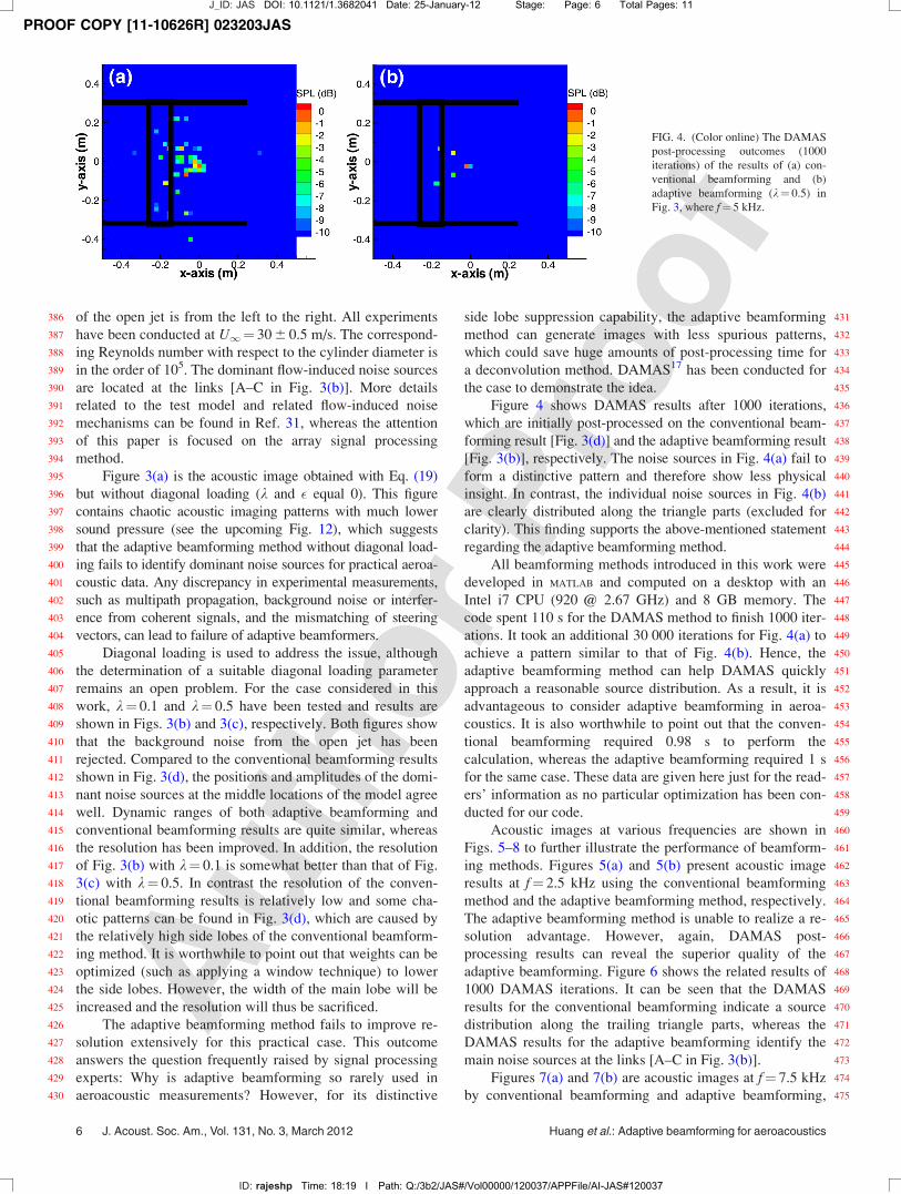
431side lobe suppression capability, the adaptive beamforming432method can generate images with less spurious patterns,433which could save huge amounts of post-processing time for434a deconvolution method. DAMAS17 has been conducted for435the case to demonstrate the idea.436Figure 4 shows DAMAS results after 1000 iterations,437which are initially post-processed on the conventional beam-438forming result [Fig. 3(d)] and the adaptive beamforming result439[Fig. 3(b)], respectively. The noise sources in Fig. 4(a) fail to440form a distinctive pattern and therefore show less physical441insight. In contrast, the individual noise sources in Fig. 4(b)442are clearly distributed along the triangle parts (excluded for443clarity). This finding supports the above-mentioned statement444regarding the adaptive beamforming method.445All beamforming methods introduced in this work were446developed in MATLAB and computed on a desktop with an447Intel i7 CPU (920 @ 2.67 GHz) and 8 GB memory. The448code spent 110 s for the DAMAS method to finish 1000 iter-449ations. It took an additional 30 000 iterations for Fig. 4(a) to450achieve a pattern similar to that of Fig. 4(b). Hence, the451adaptive beamforming method can help DAMAS quickly452approach a reasonable source distribution. As a result, it is453advantageous to consider adaptive beamforming in aeroa-454coustics. It is also worthwhile to point out that the conven-455tional beamforming required 0.98 s to perform the456calculation, whereas the adaptive beamforming required 1 s457for the same case. These data are given here just for the read-458ers’ information as no particular optimization has been con-459ducted for our code.460Acoustic images at various frequencies are shown in461Figs. 5–8 to further illustrate the performance of beamform-462ing methods. Figures 5(a) and 5(b) present acoustic image463results at f¼ 2.5 kHz using the conventional beamforming464method and the adaptive beamforming method, respectively.465The adaptive beamforming method is unable to realize a re-466solution advantage. However, again, DAMAS post-467processing results can reveal the superior quality of the468adaptive beamforming. Figure 6 shows the related results of4691000 DAMAS iterations. It can be seen that the DAMAS470results for the conventional beamforming indicate a source471distribution along the trailing triangle parts, whereas the472DAMAS results for the adaptive beamforming identify the473main noise sources at the links [A–C in Fig. 3(b)].474Figures 7(a) and 7(b) are acoustic images at f¼ 7.5 kHz475by conventional beamforming and adaptive beamforming,

FIG. 4. (Color online) The DAMAS

post-processing outcomes (1000

iterations) of the results of (a) con-

ventional beamforming and (b)

adaptive beamforming (k¼ 0.5) in

Fig. 3, where f¼ 5 kHz.

J_ID: JAS DOI: 10.1121/1.3682041 Date: 25-January-12 Stage: Page: 6 Total Pages: 11

ID: rajeshp Time: 18:19 I Path: Q:/3b2/JAS#/Vol00000/120037/APPFile/AI-JAS#120037

6 J. Acoust. Soc. Am., Vol. 131, No. 3, March 2012 Huang et al.: Adaptive beamforming for aeroacoustics

PROOF COPY [11-10626R] 023203JAS

FIG. 5. (Color online) Acoustic

image results of the practical aeroa-

coustic case, (a) the conventional

beamforming method [with Eq.

(12)] and (b) the adaptive beam-

forming method [with Eq. (19)] with

diagonal loading at k¼ 0.5, where

f¼ 2.5 kHz.

FIG. 6. (Color online) The DAMAS

post-processing outcomes (1000 iter-

ations) of the results of (a) conven-

tional beamforming and (b) adaptive

beamforming (k¼ 0.5) in Fig. 5,

where f¼ 2.5 kHz.

FIG. 7. (Color online) Acoustic

image results of the practical aeroa-

coustic case, (a) the conventional

beamforming method [with Eq.

(12)] and (b) the adaptive beam-

forming method [with Eq. (19)] with

diagonal loading at k¼ 0.5, where

f¼ 7.5 kHz.

FIG. 8. (Color online) The DAMAS

post-processing outcomes (1000

iterations) of the results of (a) con-

ventional beamforming and (b)

adaptive beamforming (k¼ 0.5) in

Fig. 7, where f¼ 7.5 kHz.

J_ID: JAS DOI: 10.1121/1.3682041 Date: 25-January-12 Stage: Page: 7 Total Pages: 11

ID: rajeshp Time: 18:19 I Path: Q:/3b2/JAS#/Vol00000/120037/APPFile/AI-JAS#120037

J. Acoust. Soc. Am., Vol. 131, No. 3, March 2012 Huang et al.: Adaptive beamforming for aeroacoustics 7

PROOF COPY [11-10626R] 023203JAS

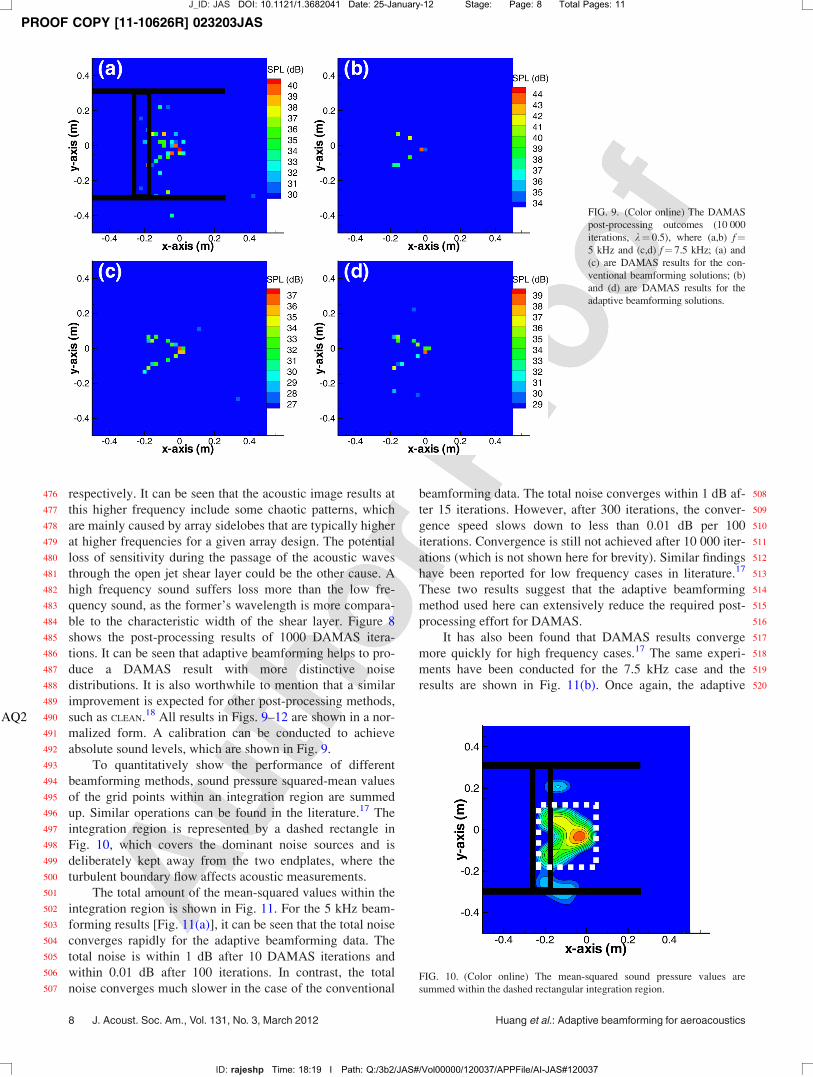
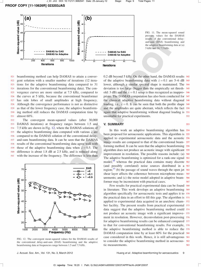
476 respectively. It can be seen that the acoustic image results at477 this higher frequency include some chaotic patterns, which478 are mainly caused by array sidelobes that are typically higher479 at higher frequencies for a given array design. The potential480 loss of sensitivity during the passage of the acoustic waves481 through the open jet shear layer could be the other cause. A482 high frequency sound suffers loss more than the low fre-483 quency sound, as the former’s wavelength is more compara-484 ble to the characteristic width of the shear layer. Figure 8485 shows the post-processing results of 1000 DAMAS itera-486 tions. It can be seen that adaptive beamforming helps to pro-487 duce a DAMAS result with more distinctive noise488 distributions. It is also worthwhile to mention that a similar489 improvement is expected for other post-processing methods,490 such as CLEAN.18 All results in Figs. 9–12AQ2 are shown in a nor-491 malized form. A calibration can be conducted to achieve492 absolute sound levels, which are shown in Fig. 9.493 To quantitatively show the performance of different494 beamforming methods, sound pressure squared-mean values495 of the grid points within an integration region are summed496 up. Similar operations can be found in the literature.17 The497 integration region is represented by a dashed rectangle in498 Fig. 10, which covers the dominant noise sources and is499 deliberately kept away from the two endplates, where the500 turbulent boundary flow affects acoustic measurements.501 The total amount of the mean-squared values within the502 integration region is shown in Fig. 11. For the 5 kHz beam-503 forming results [Fig. 11(a)], it can be seen that the total noise504 converges rapidly for the adaptive beamforming data. The505 total noise is within 1 dB after 10 DAMAS iterations and506 within 0.01 dB after 100 iterations. In contrast, the total507 noise converges much slower in the case of the conventional

508beamforming data. The total noise converges within 1 dB af-509ter 15 iterations. However, after 300 iterations, the conver-510gence speed slows down to less than 0.01 dB per 100511iterations. Convergence is still not achieved after 10 000 iter-512ations (which is not shown here for brevity). Similar findings513have been reported for low frequency cases in literature.17

514These two results suggest that the adaptive beamforming515method used here can extensively reduce the required post-516processing effort for DAMAS.517It has also been found that DAMAS results converge518more quickly for high frequency cases.17 The same experi-519ments have been conducted for the 7.5 kHz case and the520results are shown in Fig. 11(b). Once again, the adaptive

FIG. 9. (Color online) The DAMAS

post-processing outcomes (10 000

iterations, k¼ 0.5), where (a,b) f¼5 kHz and (c,d) f¼ 7.5 kHz; (a) and

(c) are DAMAS results for the con-

ventional beamforming solutions; (b)

and (d) are DAMAS results for the

adaptive beamforming solutions.

FIG. 10. (Color online) The mean-squared sound pressure values are

summed within the dashed rectangular integration region.

J_ID: JAS DOI: 10.1121/1.3682041 Date: 25-January-12 Stage: Page: 8 Total Pages: 11

ID: rajeshp Time: 18:19 I Path: Q:/3b2/JAS#/Vol00000/120037/APPFile/AI-JAS#120037

8 J. Acoust. Soc. Am., Vol. 131, No. 3, March 2012 Huang et al.: Adaptive beamforming for aeroacoustics

PROOF COPY [11-10626R] 023203JAS

521 beamforming method can help DAMAS to attain a conver-522 gent solution with a smaller number of iterations (12 itera-523 tions for the adaptive beamforming data compared to 31524 iterations for the conventional beamforming data). The con-525 vergence curves are more similar at 7.5 kHz, compared to526 the curves at 5 kHz, because the conventional beamformer527 has side lobes of small amplitudes at high frequency.528 Although the convergence performance is not as distinctive529 as that of the lower frequency case, the adaptive beamform-530 ing method still reduces the DAMAS computation time by531 almost 60%.532 The convergent mean-squared values (after 30,000533 DAMAS iterations) at frequency ranges between 1.5 and534 7.5 kHz are shown in Fig. 12, where the DAMAS solutions of535 the adaptive beamforming data computed with various k are536 compared to the DAMAS solution of the conventional delay-537 and-sum beamforming data. It can be seen that the DAMAS538 results of the conventional beamforming data agree well with539 those of the adaptive beamforming data when k¼ 0.5. The540 difference is about 1.8 dB at 2.5 kHz, and is reduced along541 with the increase of the frequency. The difference is less than

5420.2 dB beyond 5 kHz. On the other hand, the DAMAS results543of the adaptive beamforming data with k¼ 0.1 are 5–6 dB544lower, although a similar spectral shape is maintained. The545deviation is too large (bigger than the empirically set thresh-546old: 3 dB) and the k¼ 0.1 setup is thus recognized as inappro-547priate. The DAMAS computation has also been conducted for548the classical adaptive beamforming data without diagonal549loading, i.e., k¼ 0. It can be seen that both the profile shape550and the amplitudes are quite aberrant, which reflects the fact551again that adaptive beamforming without diagonal loading is552unsuitable for practical experiments.

553V. SUMMARY

554In this work an adaptive beamforming algorithm has555been proposed for aeroacoustic applications. This algorithm is556applied to experimental aeroacoustic data and the acoustic557image results are compared to that of the conventional beam-558forming method. It can be seen that the adaptive beamforming559algorithm does not produce an acoustic image with significant560improvement in resolution. The possible reasons include: (a)561The adaptive beamforming is optimized for a rank-one signal562model,29 whereas the practical data contains many discrete563(and possibly correlated) noise sources distributed in a564region;13 (b) the passage of sound waves through the open jet565shear layer affects the coherence between microphone meas-566urements; and (c) the noise model adopted in adaptive beam-567former may be inconsistent with practical cases.568Few results for practical experimental data can be found569in literature. This work develops an adaptive beamforming570algorithm specifically for aeroacoustic tests and applies it to571the practical data in an effort to fill this gap. The algorithm is572applied to experimental data acquired in an anechoic cham-573ber facility. The present results from practical experimental574data suggest that the adaptive beamforming method could575not produce an acoustic image with a significant improve-576ment in resolution. However, deconvolution post-processing577for adaptive beamforming results can be enhanced compared578to that for conventional beamforming results. For example,579the adaptive beamforming method is able to reduce the580DAMAS computation time by at least 60% for the practical581case considered in this work. Hence, it is still advantageous582to consider the adaptive beamforming method in aeroacous-583tic measurements.

FIG. 11. The mean-squared sound

pressure values for the DAMAS

results of the conventional delay-

and-sum (DAS) beamforming and

the adaptive beamforming data at (a)

5 kHz and (b) 7.5 kHz.

FIG. 12. The convergent mean-squared values for the DAMAS results of

the conventional delay-and-sum (DAS) beamforming and the adaptive

beamforming data at frequencies range between 1.5 and 7.5 kHz.

J_ID: JAS DOI: 10.1121/1.3682041 Date: 25-January-12 Stage: Page: 9 Total Pages: 11

ID: rajeshp Time: 18:20 I Path: Q:/3b2/JAS#/Vol00000/120037/APPFile/AI-JAS#120037

J. Acoust. Soc. Am., Vol. 131, No. 3, March 2012 Huang et al.: Adaptive beamforming for aeroacoustics 9

PROOF COPY [11-10626R] 023203JAS

584 ACKNOWLEDGMENTS

585 The majority of this research was supported by the586 National Science Foundation grant of China (Grant Nos.587 11172007, 11050110109, and 11110072). The experiments588 were conducted at ISVR, University of Southampton. We589 acknowledge Professor Xin Zhang for his support in the590 experiments.591

592 1D. R. Morgan and T. M. Smith, “Coherence effects on the detection593 performance of quadratic array processors, with applications to large-594 array matched-field beamforming,” J. Acoust. Soc. Am. 87, 737–747595 (1990).596 2D. E. Dudgeon, “Fundamentals of digital array processing,” Proc. IEEE597 65, 898–904 (1977).598 3Y. Liu, A. R. Quayle, A. P. Dowling, and P. Sijtsma, “Beamforming cor-599 rection for dipole measurement using two-dimensional microphone600 arrays,” J. Acoust. Soc. Am. 124, 182–191 (2008).601 4H. C. Shin, W. R. Graham, P. Sijtsma, C. Andreou, and A. C. Faszer,602 “Implementation of a Phased Microphone array in a closed-section wind603 tunnel,” AIAA J. 45, 2897–2909 (2007).604 5R. A. Gramann and J. W. Mocio, “Aeroacoustic measurements in wind605 tunnels using adaptive beamforming methods,” J. Acoust. Soc. Am. 97,606 3694–3701 (1995).607 6X. Huang, S. Chan, X. Zhang, and S. Gabriel, “Variable structure model608 for flow-induced tonal noise control with plasma actuators,” AIAA J. 46,609 241–250 (2008).610 7X. X. Chen, X. Huang, and X. Zhang, “Sound radiation from a bypass611 duct with bifurcations,” AIAA J. 47, 429–436 (2009).612 8M. J. Lighthill, “On sound generated aerodynamically. I. General theory,”613 Proc. R. Soc. London Ser. A 221, 564–587 (1952).614 9P. T. Soderman and C. S. Allen, “Microphone measurements in and out of615 stream,” in Aeroacoustic Measurements, edited by T. J. E. Mueller616 (Springer, New York, 2002), Chap. 1, pp. 26–41.617 10B. D. Van Veen and K. M. Buckley, “Beamforming: A versatile approach618 to spatial filtering,” IEEE ASSP Mag. 5, 4–24 (1988).619 11M. C. Remillieux, E. D. Crede, H. E. Camargo, R. A. Burdisso, W. J.620 Devenport, M. Rasnick, P. V. Seeters, and A. Chou, “Calibration and dem-621 onstration of the new Virginia Tech anechoic wind tunnel,” 14th AIAA/622 CEAS Aeroacoustics Conference and 29th AIAA Aeroacoustics Confer-623 ence, Vancouver, May 2008, AIAA Paper No. 2008-2911.624 12E. Sarradj, C. Fritzsche, T. Geyer, and J. Giesler, “Acoustic and aerody-625 namic design and characterization of a small-scale aeroacoustic wind626 tunnel,” Appl. Acoust. 70, 1073–1080 (2009).627 13X. Huang, “Real-time algorithm for acoustic imaging with a microphone628 array,” J. Acoust. Soc. Am. 125, EL190–EL195 (2009).

62914X. Huang, I. Vinogradov, L. Bai, and J. C Ji, “Observer for phased micro-630phone array signal processing with nonlinear output,” AIAA J. 48,6312702–2705 (2010).63215L. Bai and X. Huang, “Observer-based beamforming algorithm for acous-633tic array signal processing,” J. Acoust. Soc. Am 130, 3803–3811 (2011).63416Y. W. Wang, J. Li, P. Stoica, M. Sheplak, and T. Nishida, “Wideband635RELAX and wideband CLEAN for aeroacoustic imaging,” J. Acoust. Soc.636Am. 115, 757–767 (2004).63717T. F. Brooks and W. M. Humphrey, “A deconvolution approach for the638mapping of acoustic sources (DAMAS) determined from phased micro-639phone arrays,” J. Sound Vib. 294, 858–879 (2006).64018P. Sijtsma, “CLEAN based on spatial source coherence,” Int. J. Aeroa-641coust. 6, 357–374 (2007).64219T. Yardibi, J. Li, P. Stoica, and L. N. Cattafesta, “Sparsity constrained643deconvolution approaches for acoustic source mapping,” J. Acoust. Soc.644Am. 123, 2631–2642 (2008).64520P. A. Ravetta, R. A. Burdisso, and W. F. Ng, “Noise source localization646and optimization of phased-array results,” AIAA J. 47, 2520–2533 (2009).64721T. Yardibi, J. Li, P. Stoica, N. S. Zawodny, and L. N. Cattafesta III, “A co-648variance fitting approach for correlated acoustic source mapping,” J.649Acoust. Soc. Am. 127, 2920–2931 (2010).65022O. L. Frost, “An algorithm for linearly constrained adaptive array proc-651essing,” Proc. IEEE 60, 926–935 (1972).65223P. Stoica, Z. S. Wang, and J. Li, “Robust Capon beamforming,” IEEE Sig-653nal Proc. Lett. 10, 172–175 (2003).65424H. Cox, R. M. Zeskind, and M. M. Owen, “Robust adaptive655beamforming,” IEEE Trans. Acoust. Speech. Sig. Proc. ASSP-35,6561365–1376 (1987).65725Z. S. Wang, J. Li, P. Stoica, T. Nishida, and M. Sheplak, “Constant-beam-658width and constant -powerwidth wideband robust Capon beamformers for659acoustic imaging,” J. Acoust. Soc. Am. 116, 1621–1631 (2004).66026Y. T. Cho and M. J. Roan, “Adaptive near-field beamforming techniques661for sound source imaging,” J. Acoust. Soc. Am. 125, 944–957 (2009).66227X. Huang, L. Bai, and I. Vinogradov, “An observer for phased microphone663array signal processing with nonlinear output,” AIAA J. 48, 2702–2705664(2010). AQ366528X. Huang, “Real-time location of coherent sound sources by the observer-666based array algorithm” Meas. Sci. Technol. 22, 065501 (2011).66729S. Shahbazpanahi, A. B. Gershman, Z. Q. Luo, and K. M. Wong, “Robust668adaptive beamforming for general-rank signal models,” IEEE Trans. Sig-669nal Process. 51, 2257–2269 (2003).67030R. G. Lorenz and S. P. Boyd, “Robust minimum variance beamforming,”671IEEE Trans. Signal Process. 53, 1684–1696 (2005).67231X. Huang, X. Zhang, and Y. Li, “Broadband flow-induced sound control673using plasma actuators,” J. Sound Vib. 329, 2477–2489 (2010).67432X. Huang and X. Zhang, “The Fourier pseudospectral time-domain675method for some computational aeroacoustics problems,” Int. J. Aeroa-676coust. 5, 279–294 (2006).

J_ID: JAS DOI: 10.1121/1.3682041 Date: 25-January-12 Stage: Page: 10 Total Pages: 11

ID: rajeshp Time: 18:20 I Path: Q:/3b2/JAS#/Vol00000/120037/APPFile/AI-JAS#120037

10 J. Acoust. Soc. Am., Vol. 131, No. 3, March 2012 Huang et al.: Adaptive beamforming for aeroacoustics