ADAPTIVE DATA-DRIVEN REGULARIZATION FORVARIATIONAL IMAGE RESTORATION IN THE BV SPACE

Hongwei Zheng and Olaf HellwichComputer Vision & Remote Sensing, Berlin University of Technology

Franklinstrasse 28/29, Sekretariat FR 3-1, D-10587 Berlinhzheng,hellwich@cs.tu-berlin.de

Keywords: Bayesian estimation, regularization, convex optimization, functions of bounded variation, linear growth func-tional, self-adjusting, parameter estimation, data-driven, hyperbolic conservation laws, image restoration.

Abstract: We present a novel variational regularization in the space of functions of Bounded Variation (BV) for adaptivedata-driven image restoration. The discontinuities are important features in image processing. The BV spaceis well adapted for the measure of gradient and discontinuities. More over, the degradation of images includesnot only random noises but also multiplicative, spatial degradations, i.e., blur. To achieve simultaneous im-age deblurring and denoising, a variable exponent linear growth functional on the BV space is extended inBayesian estimation with respect to deblurring and denoising. The selectionof regularization parameters isself-adjusting based on spatially local variances. Simultaneously, the linear and non-linear smoothing oper-ators are continuously changed following the strength of discontinuities. The time of stopping the processis optimally determined by measuring the signal-to-noise ratio. The algorithm isrobust in that it can handleimages that are formed with different types of noises and blur. Numerical experiments show that the algorithmachieves more encouraging perceptual image restoration results.

1 INTRODUCTION

The primary goal of image restoration is to recoverlost information from a degraded image and obtainthe best estimate to the original image. Its applica-tions include photography, remote sensing, medicalimaging, and multimedia processing. According tothe image degradation modelg = h f + η, given anobserved image functiong ∈ L2(Ω), with Ω ⊂ R

2 isan open bounded domain, the problem is to estimatethe original imagef with unknown noiseη and pointspread functionh. In order to solve this ill-posed in-verse problem, one of the well-known techniques isby energy minimization and regularization.

In classical Sobolev spaces, we can not make de-tailed analysis and reasonable measure of discontinu-ities. A simple image including a white disk on ablack background is not in any Sobolev space, but be-longs to the BV space. The BV space is the spaceof functions for which the sum of the perimeters ofthe level sets is finite. Therefore, the BV space iswell adapted for determining discontinuities across or

along edges. Compared to wavelet based methods inthe frequency domain (Gousseau and Morel, 2001),the assumption of the functions on the BV space isstill too restrictive to represent tiny detailed texturesand infinite discontinuities (Alvarez and Gousseau,1999). However, currently, the BV space is still amuch larger space than the Sobolev space for mod-eling images in the spatial domain.

Since the seminal work of the ROF model (Rudinet al., 1992), the BV space based functionals havebeen widely applied to image restoration, super-resolution approaches, segmentation and related earlyvision tasks, e.g., Mumford-Shah functional (Mum-ford and Shah, 1989), modeling of oscillatory com-ponents (Meyer, 2001), modeling of inpainting andsuper-resolution approaches, (Chan and Shen, 2006).Recently, (Aubert and Vese, 1997), (Vese, 2001)propose a convex linear growth functional in theBV space for deblurring and denoising usingΓ-convergence approximation. (Chen et al., 2006),(Chen and Rao, 2003) suggest a more general variableexponent, linear growth functional in the BV space

53

for image denoising. However, through the literaturestudy, we find that only little work is done on howto determine regularization parameters, and diffusionoperators for achieving optimal and high-fidelity im-age restoration results.

In this paper, we extend the variable exponent,linear growth functional (Chen et al., 2006), (Chenand Rao, 2003) to double regularized Bayesian es-timation for simultaneously deblurring and denois-ing. The Bayesian framework provides a structuredway to include prior knowledge concerning the quan-tities to be estimated (Freeman and Pasztor, 2000).Different from traditional “passive” edge-preservingmethods (Geman and Reynolds, 1992), our methodis an “active” data-driven approach which integratesself-adjusting regularization parameters and dynamiccomputed gradient prior for self-adjusting the fidelityterm and multiple image diffusion operators. A newscheme is designed to select the regularization pa-rameters adaptively on different levels based on themeasurements of local variances. The chosen diffu-sion operators are automatically adjusted followingthe strengths of edge gradient. The suggested ap-proach has several important effects: firstly, it showsa theoretically and experimentally sound way of howlocal diffusion operators are changed automaticallyin the BV space. Secondly, the self-adjusting regu-larization parameters also control the diffusion oper-ators simultaneously for image restoration. Finally,this process is relatively simple and can be easily ex-tended for other regularization or energy optimiza-tion approaches. The experimental results show thatthe method yields encouraging results under differentkinds and amounts of noise and degradation.

The paper is organized as follows. In section 2, wediscuss the concepts of BV space, the total variation(TV) model and its related functionals. In section 3,we present a Bayesian estimation based adaptive vari-ational regularization with respect to the estimationof PSFs and images. Numerical approximation andexperimental results are shown in section 4. Conclu-sions are summarized in section 5.

2 RELATED WORK

2.1 The Bv Space and the Tv Method

Following the total variation (TV) functional (Rudinet al., 1992), (Chambolle and Lions, 1997), (Weickertand Schnorr, 2001), (Chan et al., 2002), (Aubert andVese, 1997), we study the total variation functional inthe bounded total variation (BV) space.

Definition 2.1.1 BV(Ω) is the subspace of functionsf ∈ L1(Ω) where the quantity is finite,

TV( f ) =Z

Ω|D f |dA= (1)

sup

ZΩ

f ·divϕdA ; ϕ ∈C1c(Ω,RN)

where dA= dxdy, |ϕ(A)|L∞(Ω) ≤ 1, C1c(Ω,RN) is

the space of functions in C1(Ω) with compact sup-port Ω. BV(Ω) endowed with the norm‖ f‖BV(Ω) =‖ f‖L1(Ω) +TV( f ) which is a Banach space.

While one adopts the TV measure for image regular-ization, the posterior energy for Tikhonov Regulariza-tion then takes the form which is also given in (Rudinet al., 1992),

J ( f ) =λ2

ZΩ|g−h f |2dA+

ZΩ|D f |dA (2)

whereg is the noisy image,f is an ideal image andλ > 0 is a scaling regularization parameter. When animage f is discontinuous, the gradient off has to beunderstood as a measure. TheTV( f ) functional isoften denoted by

RΩ |D f |dxdy, with the symbolD re-

ferring to the conventional differentiation∇. One usef ∈ L1(Ω) to simplify the numerical computation (see(Giusti, 1984), for instance),

RΩ |D f |dA=

RΩ |∇ f |dA.

In order to study more precisely the influence ofthe smoothing term in the regularization, we need tomake an insight observation of a more general totalvariation functional which can help us to understandthe convexity criteria in variational regularization. Ageneral bounded total variational functional can bewritten in the following,

J ( f(g,h)) =λ2

ZΩ

(g−h f)2dA+

ZΩ

φ(|∇ f (x,y)|)dA

The choice of the functionφ is crucial. It determinesthe smoothness of the resulting functionf in the spaceV = f ∈ L2(Ω);∇ f ∈ L1(Ω) which is not reflexive.

In this variational energy function, the closenessof the solution to the data is imposed by the penaltyterm φ(·) in the energy function. If the energy func-tions are nonconvex, it might become more compli-cated than the convex functionals. Although somenon-convexφ(·) penalty terms can achieve edge-preserving results, convex penalty terms can help usto get a global convergence and decrease the complex-ity of computation. In the following, we studyφ(·) ina more general formφ(∇ f )→ φ(D f ) in the BV space.

2.2 Convex Linear-Growth Functional

Let Ω be an open, bounded, and connected subsetof R

N. We use standard notations for the Sobolev

VISAPP 2007 - International Conference on Computer Vision Theory and Applications

54

W1,p(Ω) and Lebesgue spacesLp(Ω). A variationalfunction can be written in the form,

J ( f(g,h)) =λ2

ZΩ

(g−h f)2dA+Z

Ωφ(D f (x,y))dA

where the functionR

Ω φ(D f )dA is finite on the spaceW1,1 which is a nonreflexive Banach space.

We recall the notation of lower semicontinuity offunctionals defined on theBV(Ω) space. We denoteby LN the LebesgueN-dimensional measureRN andby H α the α-dimensional Hausdorff measure. Wesay that f ∈ L1(Ω) is a function of bounded varia-tion ( f ∈ BV(Ω)) if its distributed derivativeD f =(D1 f , ...,DN f ) belongs to the weakest topology onM (Ω). M (Ω) is the set of all signed measures onΩ with bounded total variation.

For any functionf ∈ L1(Ω), we denote bySf thecomplement of the Lebesgue set off . The setSf isof zero Lebesgue measure and is also called thejumpset of f. If f ∈ BV(Ω), then f is differentiable al-most everywhere onΩ\Sf . Moreover, the Hausdorffdimension ofSf is at most(N− 1) and forH N−1,x∈ Sf it is possible to find uniquef +(x), f−(x) ∈ R,with f +(x) > f−(x) andν ∈ SN−1 of unit sphere inR

N, such that

limr→0+

r−NZ

Bνr (x)

| f (y)− f +(y)|dy

= limr→0+

r−NZ

Bνr (x)

| f (y)− f−(y)|dy= 0 (3)

where Bνr (x) = y ∈ Br(x) : (y − x) · ν > 0 and

B−νr (x) = y ∈ Br(x) : (y− x) · ν < 0. The normal

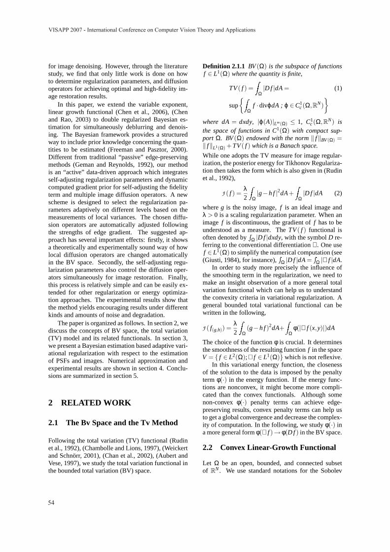
ν means that they points toward the larger value inthe imagef . We denote byBr(x) the ball centered inx of radiusr, shown in Fig. 1.

We have the Lebesgue decomposition,

D f = ∇ f ·LN +Ds f (4)

where∇ f ∈ (L1(Ω))N is the Radon-Nikodym deriva-tive of D f with respect toLN. In other words,∇ fis the density of the absolutely continuous part ofD f with respect to the Lebesgue measure. We alsohave the decomposition forDs f = Cf + Jf , whereJf = ( f + − f−)Nf ·H

N−1S is Hausdorff partor jump

part andCf is theCantor partof D f . The measureCf is singular with respect toLN and it is diffuse, thatis, Cf (S) = 0 for every setSof Hausdorff dimensionN−1. H N−1

|Sfis called the perimeter of related edges

in Ω. Finally, we can writeD f and its total variationon Ω, |D f |(Ω), in the following,

D f = ∇ f ·LN +Cf +( f +− f−)ν ·H N−1|Sf

|D f | =Z

Ω|∇ f |dx+

ZΩ\Sf

|Cf |+Z

Sf

( f + − f−)dH N−1|Sf

( )fn x

fS

( )r

B xx

( )xf

( )xf

Figure 1: Definition off +, f−, and the jump setSf .

It is then possible to define the convex function ofmeasureφ(| · |) onM (Ω), which is forD f ,

φ(|D f |) = φ(|∇ f |) ·LN +φ∞(1)|Ds f |, (5)

and the functional following (Goffman and Serrin,1964),Z

Ωφ(|D f |) =

ZΩ

φ(|∇ f |)dx+Z

Ωφ∞(1)|Ds f |, (6)

where the functionalφ(| · |)(Ω) is proved in weaktopology and lower semi-continuous onM (Ω). Thatis to say that

RΩ φ(|D f |) is convex onBV(Ω), φ is

convex and increasing onR+.By the decomposition ofDs f , the properties ofCf ,

Jf , and the definition of the constantc, the functionalRΩ φ(|D f |) can be written as,ZΩ

φ(|D f |) =Z

Ωφ(|∇ f |)dx

+ cZ

Ω\Sf

|Cf |+cZ

Sf

( f + − f−)dH N−1|Sf

Based on this equation, the energy functional on theBV space becomes,

inff∈BV(Ω)

J =λ2

ZΩ

(g−h f)2dA+Z

Ωφ(|D f |)dA (7)

Although some characterization of the solution is pos-sible in the distributional sense, it remains difficultto handle numerically. To circumvent the problem,(Vese, 2001) approximates the BV solution using thenotion of Γ-convergence which is also an approxi-mation for the well-known Mumford-Shah functional(Mumford and Shah, 1989). The Mumford-Shahfunctional is a sibling of this functional (Chan andShen, 2006).

The target of studying these functionals on the BVspace is to understand a more general variable expo-nent,Lp linear growth functional which is a deductionfunctional on the BV space.

2.3 Variable Exponent Linear-GrowthFunctional

While the penalty function isφ(|D f |)→ φ(x, |D f |), itbecomes a variable exponent linear growth functional

ADAPTIVE DATA-DRIVEN REGULARIZATION FOR VARIATIONAL IMAGE RESTORATION IN THE BV SPACE

55

in the BV space (Chen et al., 2006), (Chen and Rao,2003),

J ( f(g,h)) =λ2

ZΩ

(g−h f)2dA+Z

Ωφ(x,D f (x,y))dA

For the definition of a convex function of measures,we refer to the works of (Goffman and Serrin, 1964),(Demengel and Teman, 1984). According to theirwork, for f ∈ BV(Ω), we have,Z

Ωφ(x,D f )dA=

ZΩ

φ(x,∇ f )dA+Z

Ω|Ds f |dA (8)

where

φ(x,∇ f )dA=

1q(x) |∇ f |q(x), |∇ f | < β

|∇ f |− βq(x)−βq(x)

q(x) , |∇ f | ≥ β

whereβ > 0 is fixed, and 1≤ q(x) ≤ 2. The termq(x) is chosen asq(x) = 1+ 1

1+k|∇Gσ∗I(x)|2based on

the edge gradients.I(x) is the observed imageg(x),Gσ(x) = 1

σ exp[−|x|2/(2σ2)] is a Gaussian filter.k >0, σ > 0 are fixed parameters. The main benefit ofthis equation is that the local image information arecomputed as prior information for guiding image dif-fusion. This functional including two equations areboth convex and semi-continuous. This leads to amathematically sound model for ensuring the globalconvergence. This equation is extended in a Bayesianestimation based double variational regularization notonly for image denoising but also for image deblur-ring.

3 BAYESIAN ESTIMATIONBASED VARIATIONAL IMAGERESTORATION

Following a Bayesian paradigm, the ideal imagef ,the PSFh and an observed imageg fulfill

P( f ,h|g) =p(g| f ,h)P( f ,h)

p(g)∝ p(g| f ,h)P( f ,h) (9)

Based on this form, our goal is to find the op-timal estimated imagef and the optimal blurkernel h that maximizes the posteriorp( f ,h|g).J ( f |h,g) = − logp(g| f ,h)P( f ) and J (h| f ,g) =− logp(g| f , h)P(h) express that the energy costJis equivalent to the negative log-likelihood of the data.

The resulting method attempts to minimize dou-ble cost functions subject to constraints such as non-negativity conditions of the image and energy preser-vation of PSFs. The objective of the convergence is tominimize double cost functions by combing the en-ergy function for the estimation of PSFs and images.

(a) (b) (c)

Figure 2: Homogeneous Neumann Boundary Conditions.(a) An original MRI head image. (b)(c) HomogeneousNeumann boundary condition is implemented by mirroringboundary pixels.

We propose a Bayesian based functional on the BVspaces. It is formulated according to

Jε( f ,h) =λ2

ZΩ

(g−h f)2dA+βZ

Ω(∇h)dA

+γZ

Ωφε(x,D f )dA (10)

The Neumann boundary condition (shown inFig. 2) ∂ f

∂N (x, t) = 0 on ∂Ω × [0,T] and the initialconditionf (x,0) = f0(x) = g in Ω are used, whereNis the direction perpendicular to the boundary.

3.1 Alternating Minimization

To avoid the scale problem between the minimizationof PSF and image via steepest descent, an AM methodfollowing the idea of coordinate descent is applied(Zheng and Hellwich, 2006). The AM algorithm de-creases complexity.

The equations derived from Eq. (10) are using fi-nite differences which approximate the flow of theEuler-Lagrange equation associated with it,

∂Jε∂ f

= λ1h(−x,−y)∗ (h∗ f −g)− γdiv(φ(x,∇ f ))

∂Jε∂h

= λ2 f (−x,−y)∗ ( f ∗h−g)−β∇h·div

(∇h|∇h|

)

Neumann boundary conditions are assumed (Acarand Vogel, 1994). In the alternate minimization,blur identification including deconvolution, and data-driven image restoration including denoising are pro-cessed alternatingly via the estimation of images andPSFs. The partially recovered PSF is the prior for thenext iterative image restoration and vice versa. Thealgorithm is described in the following:

Initialization:g(x) = g(x), h0(x) is random numberswhile nmse> threshold

(1). nth it. fn(x) = argmin( fn|hn−1,g),fix hn−1(x), f (x) > 0

(2). (n+1)th it. hn+1 = argmin(hn+1| fn,g),fix fn(x), h(x) > 0

end

VISAPP 2007 - International Conference on Computer Vision Theory and Applications

56

While h = I and I is the identity matrix, the al-ternating minimization of PSFs and images becomesthe estimation of images, e.g., it is corresponding to adenoising problem. Whileh 6= I (h is generally a con-volution operator), it corresponds to a deblurring anddenoising problem. The existence and uniqueness ofsolution remain true, ifh satisfies the following hy-potheses: (a)h is a continuous and linear operatoron L2(Ω). (b) h does not annihilate constant func-tions. (c)h is injective. Thereby, we need to considerthe blur kernels at the first step. Further more, we dodeconvolution for the blurred noisy image. Then thedeconvolved image is smoothed by a family of lin-ear and nonlinear diffusion operators in an alternatingminimization.

3.2 Self-Adjusting RegularizationParameters

We have classified the regularization parametersλ inthree different levels. Here, we present the method forthe selection of window-based regularization param-etersλw (window w basedλw, the 1st level). Whenthe size of windows is amplified to the size of an in-put image,λ becomes a scale regularization param-eter for the whole image (the 2nd level). If we fixλ for the whole process, then the selection of regu-larization parameter is conducted on the level of onefixed λ for the whole process (the 3nd level). We as-sume that the noise is approximated by additive whiteGaussian noise with standard deviationσ to constructa window-based local variance estimation. Then wefocus on the adjustment of parameterλ and operatorsin the smoothing termφ. These two computed compo-nents can be prior knowledge for preserving disconti-nuities and detailed textures during image restoration.The Eq. 10 can be formulated in the following,

argminZ

Ωφ(x,D f (x,y))dAsubject to

ZΩ

(g−h f)2dA

where the noise is a Gaussian distributed with vari-anceσ2. λ can be a Lagrange multiplier in the fol-lowing form,

λ =1

σ2|Ω|

ZΩ

div [φ(x,D f (x,y))] (g−h f)dA (11)

λ is a regularization parameter controlling the “bal-ance” between the fidelity term and the penalty term.The underlying assumption of this functional satisfies‖ f‖BV(Ω) = ‖ f‖L1(Ω) + TV( f ) in the BV space. Thedistributed derivative|D f | generates an approxima-tion of input “cartoon model”and oscillation model(Meyer, 2001). Therefore, this process preservesdiscontinuities during the elimination of oscillatory

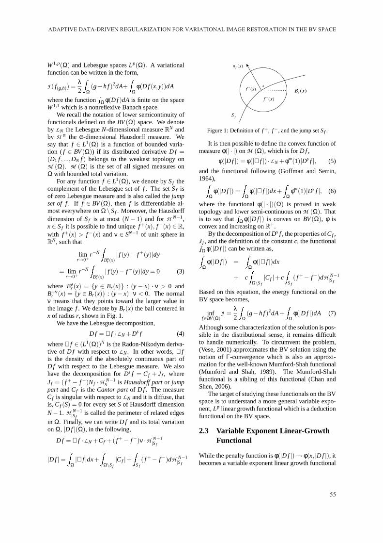
Figure 3: a|b. (a) Computedλ ∈ [0.012,0.032] values insampling windows for the image with size [160, 160]. (b)Zoom in (a) for showing the distribution of the regulariza-tion parametersλw.

noise. We note that the termR

Ω (g−h f)2dA is thepower of the residue. Therefore, there exists a re-lationship among the non-oscillatory sketch “cartoonmodel” (Mumford and Shah, 1989), (Blake and Zis-serman, 1987), oscillation model (Meyer, 2001) andthe reduced power of the original image with someproportional measure. We formulate the local vari-anceLw(x,y) in a given windoww based on an inputimage.

Lw(x,y) =1|Ω|

ZΩ[ fw(x,y)−E( fw)]2w(x,y)dxdy (12)

wherew(x,y) is a normalized and symmetric smallwindow, fw is the estimated image in a small windoww. E( fw) is the expected value with respect to thewindow w(x,y) on the size ofΩ×Ω estimated im-age f in each iteration. The local variance in a smallwindow satisfiesvar( fw) = Lw(x,y). Thereby, we canwrite λ for a small windoww according to Euler-Lagrange equation for the variation with respect tofTherefore, the regularization equation is with respectto the window-levels. It becomes

Jε( f ) = ∑λwLw(x,y)+Sp( f ) (13)

whereλwis a λ in a small windoww, Sp( f ) is thesmoothing term. Thus, we can easily get manyλw formoving windows which can be adjusted by local vari-ances, shown in Fig. 3. Theseλw are directly usedas regularization parameters for adjusting the balanceduring the energy optimization. They also adjust thestrength of diffusion operators for keeping more fi-delity during the diffusion process. The related regu-larization parametersβ andγ incorporate theλ, whilethe parameterλ of the fidelity term needs to be de-fined.

During image restoration, the parameterλ can beswitched among three different levels. The window-based parameterλw and the scale-based (entire im-age) parameter can be adjusted to find the optimalresults. Simultaneously,λ thus control the image fi-delity and diffusion strength of each selected operatorin an optimal manner.

ADAPTIVE DATA-DRIVEN REGULARIZATION FOR VARIATIONAL IMAGE RESTORATION IN THE BV SPACE

57

(a) (b)

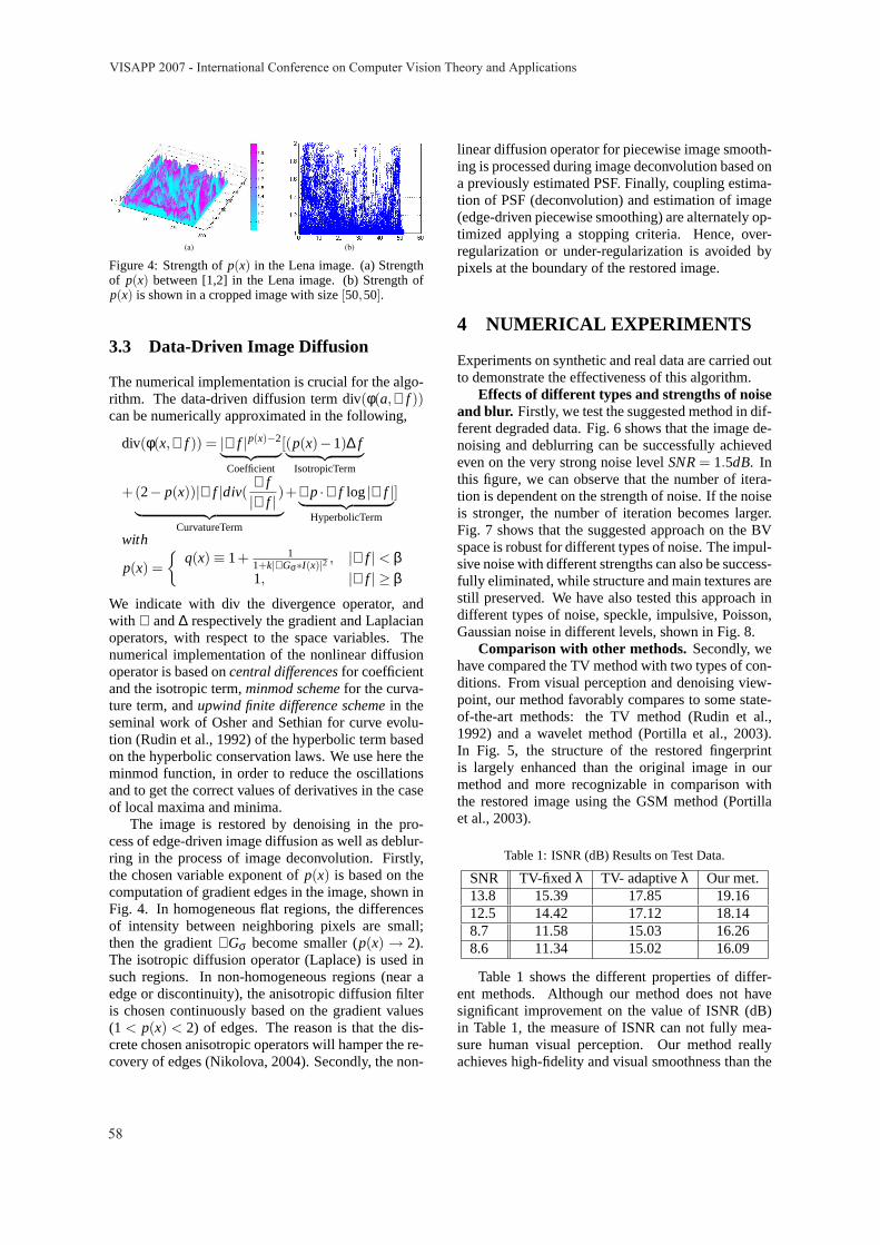
Figure 4: Strength ofp(x) in the Lena image. (a) Strengthof p(x) between [1,2] in the Lena image. (b) Strength ofp(x) is shown in a cropped image with size[50,50].

3.3 Data-Driven Image Diffusion

The numerical implementation is crucial for the algo-rithm. The data-driven diffusion term div(φ(a,∇ f ))can be numerically approximated in the following,

div(φ(x,∇ f )) = |∇ f |p(x)−2

︸ ︷︷ ︸

Coefficient

[(p(x)−1)∆ f︸ ︷︷ ︸

IsotropicTerm

+(2− p(x))|∇ f |div(∇ f|∇ f |

)

︸ ︷︷ ︸

CurvatureTerm

+∇p·∇ f log|∇ f |︸ ︷︷ ︸

HyperbolicTerm

]

with

p(x) =

q(x) ≡ 1+ 1

1+k|∇Gσ∗I(x)|2, |∇ f | < β

1, |∇ f | ≥ β

We indicate with div the divergence operator, andwith ∇ and∆ respectively the gradient and Laplacianoperators, with respect to the space variables. Thenumerical implementation of the nonlinear diffusionoperator is based oncentral differencesfor coefficientand the isotropic term,minmod schemefor the curva-ture term, andupwind finite difference schemein theseminal work of Osher and Sethian for curve evolu-tion (Rudin et al., 1992) of the hyperbolic term basedon the hyperbolic conservation laws. We use here theminmod function, in order to reduce the oscillationsand to get the correct values of derivatives in the caseof local maxima and minima.

The image is restored by denoising in the pro-cess of edge-driven image diffusion as well as deblur-ring in the process of image deconvolution. Firstly,the chosen variable exponent ofp(x) is based on thecomputation of gradient edges in the image, shown inFig. 4. In homogeneous flat regions, the differencesof intensity between neighboring pixels are small;then the gradient∇Gσ become smaller (p(x) → 2).The isotropic diffusion operator (Laplace) is used insuch regions. In non-homogeneous regions (near aedge or discontinuity), the anisotropic diffusion filteris chosen continuously based on the gradient values(1 < p(x) < 2) of edges. The reason is that the dis-crete chosen anisotropic operators will hamper the re-covery of edges (Nikolova, 2004). Secondly, the non-

linear diffusion operator for piecewise image smooth-ing is processed during image deconvolution based ona previously estimated PSF. Finally, coupling estima-tion of PSF (deconvolution) and estimation of image(edge-driven piecewise smoothing) are alternately op-timized applying a stopping criteria. Hence, over-regularization or under-regularization is avoided bypixels at the boundary of the restored image.

4 NUMERICAL EXPERIMENTS

Experiments on synthetic and real data are carried outto demonstrate the effectiveness of this algorithm.

Effects of different types and strengths of noiseand blur. Firstly, we test the suggested method in dif-ferent degraded data. Fig. 6 shows that the image de-noising and deblurring can be successfully achievedeven on the very strong noise levelSNR= 1.5dB. Inthis figure, we can observe that the number of itera-tion is dependent on the strength of noise. If the noiseis stronger, the number of iteration becomes larger.Fig. 7 shows that the suggested approach on the BVspace is robust for different types of noise. The impul-sive noise with different strengths can also be success-fully eliminated, while structure and main textures arestill preserved. We have also tested this approach indifferent types of noise, speckle, impulsive, Poisson,Gaussian noise in different levels, shown in Fig. 8.

Comparison with other methods. Secondly, wehave compared the TV method with two types of con-ditions. From visual perception and denoising view-point, our method favorably compares to some state-of-the-art methods: the TV method (Rudin et al.,1992) and a wavelet method (Portilla et al., 2003).In Fig. 5, the structure of the restored fingerprintis largely enhanced than the original image in ourmethod and more recognizable in comparison withthe restored image using the GSM method (Portillaet al., 2003).

Table 1: ISNR (dB) Results on Test Data.

SNR TV-fixed λ TV- adaptiveλ Our met.13.8 15.39 17.85 19.1612.5 14.42 17.12 18.148.7 11.58 15.03 16.268.6 11.34 15.02 16.09

Table 1 shows the different properties of differ-ent methods. Although our method does not havesignificant improvement on the value of ISNR (dB)in Table 1, the measure of ISNR can not fully mea-sure human visual perception. Our method reallyachieves high-fidelity and visual smoothness than the

VISAPP 2007 - International Conference on Computer Vision Theory and Applications

58

Figure 5: a|b|cd|e| f . Comparison of two methods for fingerprint

denoising. (a)(d) Cropped noisy image,SNR= 8 dB. (b)(e)GSM method (Portilla et al., 2003) PSNR=27.8. dB. (c)(f)The suggested method PSNR= 28.6 dB.

SNR 1.5 dB 100 Iteration 200 Iteration 300 Iteration

400 Iteration 500 Iteration 550 Iteration 580 Iteration

Noise image, SNR = 1.5dB, sigma 75 Restored Image using the suggested method

Figure 6: Restored image using the suggested method.Stronger distributed noise withSNR= 1.5dB. 100 itera-tions need 600 seconds for the image size of [512,512].

TV methods. The TV methods with fixedλ and adap-tive λ still have some piecewise constant effects on re-stored images. Furthermore, our method keeps high-fidelity for restoring stronger or impulsive noisy im-ages, while the TV methods (fixedλ and adaptiveλ)cannot keep high-fidelity for restoring such degradedimages, e.g., SNR = 1.5dB or some impulsive noisyimages, shown in Fig. 6, Fig. 7 and Fig. 8.

More results are shown in Fig. 9 to demonstratethat the suggested method keeps high-fidelity and vi-sual perception image restoration. These experimentsshow that the suggested method on the BV spacehas some advantages on image denoising and image

Figure 7: a|b|c|de| f |g|h . Restoration of impulsive noise images.

(a) 10% salt-pepper noise image. (b) Restored image, 200iterations. (c)(d) Zoom in images from (a)(b) respectively.(e)25% salt-pepper noise image. (f) Restored image, 900iterations. (g)(h) Zoom in images from (e)(f) respectively.

Figure 8: a|b|c|de| f |g|h . Image denoising using the suggested

method. (a)(b)Speckle noise image and denoising. (c)(d)Zoom in from (a)(b) respectively, 100 iterations. (e)(f) Pois-son noise image and denoising. (g)(h) Zoom in from (e)(f)respectively, 100 iteration.

restoration. It can also be easily extended to other re-lated early vision problems.

5 CONCLUSION

The main structure and skeleton of images are wellapproximated on the BV space. In order to preservetextures and detailed structures, more constraints orgenerative prior information are investigated. Wehave developed a self-adjusting scheme that controlsthe image restoration based on the edge-driven con-vex semi-continuous functionals. The performanceof image restoration is not only based on the com-puted gradient but also based on local variances ofthe residues. Therefore, linear and nonlinear smooth-ing operators in the smoothing term are continuouslyself-adjusting via the gradient power. The consistencyof self-adjusting local variances and the global con-vergence can be achieved in the iterative convex op-timization approach. We have shown that this algo-rithm has relatively robust performance for differenttypes and strengths of noise. The image restorationkeeps high fidelity to the original image.

ADAPTIVE DATA-DRIVEN REGULARIZATION FOR VARIATIONAL IMAGE RESTORATION IN THE BV SPACE

59

(a) (b) (c)

Figure 9: Image denoising using the suggested method. (a)column: Original images. (b) column: Noisy images withSNR = 10 dB . (c) column: Restored images (100 iterations)using the suggested method.

REFERENCES

Acar, R. and Vogel, C. R. (1994). Analysis of boundedvaraition penalty methods for ill-posed problems.In-verse problems, 10(6):1217–1229.

Alvarez, L. and Gousseau, Y. (1999). Scales in naturalimages and a consequence on their bounded varia-tion norm. InScale-Space, volume Lectures Notes onComputer Science, 1682.

Aubert, l. and Vese, L. (1997). A variational methodin image recovery. SIAM Journal Numer. Anal.,34(5):1948–1979.

Blake, A. and Zisserman, A. (1987).Visual Reconstruction.MIT Press, Cambridge.

Chambolle, A. and Lions, P. L. (1997). Image recoveryvia total variation minimization and related problems.Numer. Math., 76(2):167–188.

Chan, T. F., Kang, S. H., and Shen, J. (2002). Euler’s elas-tica and curvature based inpaintings.SIAM J. Appli.Math, pages 564–592.

Chan, T. F. and Shen, J. (2006). Theory and computa-tion of variational image deblurring.Lecture Notes on“Mathematics and Computation in Imaging Scienceand Information Processing”.

Chen, Y., Levine, S., and Rao, M. (2006). Variable expo-nent, linear growth functionals in image restoration.SIAM Journal of Applied Mathematics, 66(4):1383–1406.

Chen, Y. and Rao, M. (2003). Minimization problems andassociated flows related to weightedp energy and to-tal variation. SIAM Journal of Applied Mathematics,34:1084–1104.

Demengel, F. and Teman, R. (1984). Convex functions of ameasure and applications.Indiana University Mathe-matics Journal, 33:673–709.

Freeman, W. and Pasztor, E. (2000). Learning low-levelvision. In Academic, K., editor,International Journalof Computer Vision, volume 40, pages 24–57.

Geman, S. and Reynolds, G. (1992). Constrained restora-tion and the recovery of discontinuities.IEEE Trans.PAMI., 14:367–383.

Giusti, E. (1984). Minimal Surfaces and Functions ofBounded Variation. Birkhauser.

Goffman, C. and Serrin, J. (1964). Sublinear functions ofmeasures and variational integrals.Duke Math. J.,31:159–178.

Gousseau, Y. and Morel, J.-M. (2001). Are natural imagesof bounded variation?SIAM Journal on MathematicalAnalysis, 33:634–648.

Meyer, Y. (2001). Oscillating patterns in image processingand in some nonlinear evolution equations.The 15thDean Jacquelines B. Lewis Memorial Lectures, 3.

Mumford, D. and Shah, J. (1989). Optimal approximationsby piecewise smooth functions and associated varia-tional problems. Communications on Pure and Ap-plied Mathematics, 42:577–684.

Nikolova, M. (2004). Weakly constrained minimization:application to the estimation of images and signalsinvolving constant regions.J. Math. Image Vision,21(2):155–175.

Portilla, J., Strela, V., Wainwright, M., and Simoncelli,E. (2003). Image denoising using scale mixtures ofGaussians in the Wavelet domain.IEEE Trans. onImage Processing, 12(11):1338–1351.

Rudin, L., Osher, S., and Fatemi, E. (1992). Nonlinear totalvarition based noise removal algorithm.Physica D,60:259–268.

Vese, L. A. (2001). A study in the BV space of a denoising-deblurring variational problem.Applied Methematicsand Optimization, 44:131–161.

Weickert, J. and Schnorr, C. (2001). A theoretical frame-work for convex regularizers in PDE-based computa-tion of image motion.International Journal of Com-puter Vision, 45(3):245–264.

Zheng, H. and Hellwich, O. (2006). Double regularizedBayesian estimation for blur identification in video se-quences. InP.J. Narayanan et al. (Eds.) ACCV, vol-ume 3852 ofLNCS, pages 943–952. Springer.

VISAPP 2007 - International Conference on Computer Vision Theory and Applications

60