Adaptive finite element methods in computational mechanicsjjan/transfer/adaptive_hansbo.pdf ·...

Computer Methods in Applied Mechanics and Engineering 101 (1992) 143-181 North-Holland

CMA 296

Adaptive finite element methods in computational mechanics

Claes Johnson and Peter Hansbo Department of Mathematics, Chalmers University of Technology, S-412 96 Gdteborg, Sweden

Received 14 October 1991

We present a general approach to adaptivity for finite element methods and give applications to linear elasticity, non-linear elasto-plasticity and nonlinear conservation laws, including numerical results.

1. Introduction

In this paper, we review the general approach to adaptivity for finite element methods presented in [l-16]. We also present new theoretical and computational results for linear elasticity, non-linear elasto-plasticity and non-linear conservation laws illustrating the general theory.

The basic problem in adaptivity for finite element methods may be formulated as follows. Suppose 9 is a given (initial-)boundary value problem with given data f and corresponding exact solution U. Let ??,, p be a finite element method for 9 based on piecewise polynominal approximation on a family { .Yh,p} of meshes with mesh functions h = h(x, t) and p = p(x, t)

giving the local mesh size h(x, t) in space and time and local order p(x, t) of the polynomial approximations as functions of space x and time t and let { uh,*} be the corresponding family of finite element solutions. Let I] * 11 b e a g iven norm and TOL > 0 a given tolerance. Then construct and algorithm & for finding a mesh Y,_, such that for the corresponding finite element solution u,,~, we have

(1 u - uh,p 11 6 TOL > (14

and the work to compute u~,~ is nearly minimal. As a measure of the computational work, for definiteness, we use the total number of unknowns. We thus seek an algorithm & for solving (approximately) the following non-linear optimization problem. Find a mesh 9;:; with as few degrees of freedom as possible, referred to as an optimal mesh, under the side condition that ]I u - u~,~ I] < TOL, where u~,~ is the corresponding finite element solution. This is a complex problem which is not directly solvable since the exact solution u is not known and the

Correspondence to: Claes Johnson, Department of Mathematics, Chalmers University of Technology and University of Goteborg, Sven Hultins gata 6, 412 96 Goteborg, Sweden.

0045-7825/92/$05.00 0 1992 Elsevier Science Publishers B.V. All rights reserved

144 C. Johnson, P. Hansbo, Adaptive finite element methods

dependence of IIu - u~,~II on (h, p) is very implicit. In general, both the local mesh size h and the local degree p of the polynomial approximation are variable in space and time and are determined in the adaptive process. We refer to adaptive algorithms in this generality as (h, p)-methods. Adaptive algorithms with p fixed or h fixed are referred to as h-methods and p-methods, respectively. In this note we mainly concentrate on h-methods, but our results also directly apply to the case of (h, p)-methods (if p is not large). Concerning h-adaptivity, note that in addition to the local mesh size, the local mesh orientation and stretching of the mesh (in space or space-time) may also be adaptively controlled. Thus, for simplicity of notation, we assume that the mesh parameter h = hfx, t) in general represents both the mesh size in space and time, as well as the mesh orientation/stretching. The main emphasis below is on methods without adaptive orientation/stretching, but cases including such features are also discussed.

Clearly we require the adaptive algorithm & to be both reliable and ejficient, in the sense that the desired error control should be guaranteed, and the computational work should be nearly minimal. The basic problem in adaptivity is to construct adaptive algorithms that are both reliable and efficient in the sense just given. Successful solutions of this problem will have a profound influence on the finite element software of tomorrow.

In our work [l-16], we have constructed reliable and efficient adaptive algorithms for a large class of problems, including elliptic, parabolic and hyperbolic problems, linear as well as non-linear. Typical applications concern convection-diffusion problems in the whole range from diffusion-dominated to convection-dominated problems, stationary as well as time- dependent problems, linear wave equations, non-linear monotone elliptic problems modelling unilateral contact and elasto-plasticity, and also non-linear conservation laws. Below we give more details and/or more precise references on these topics.

Our algorithms are based on a posteriori error estimates of the form

lb - uh,ptl d E,th, P, 'h,p, f> ) (1.2)

where the error If u - u~,~ II is estimated in terms of a directly computable quantity E,(h, p, u~,~, f) depending on the computed solution u~,~, the mesh size h(n, t) and the degree p(x, t) of the polynomial approximation, and the data f of the problem. The dependence in E, on the computed solution u~,~ yp t ically occurs through the residual R(u,,,)

Of uh p, which is basically the deviation from equality (properly evaluated) obtained by inserting u~,~ into the given continuous equation. For elliptic problems, (1.2) may typically take the form

11 u - uh,plj G ‘11 h2R(uh,,)ll or

IlV(u - UhJl zz mw+z,,)ll ’

(1.3)

where 11. II may be the &-norm or an L,-norm, 1 G q s ~0, or weighted such norms, and where C is a certain constant to be commented on below. For first order hyperbolic problems, (1.2) may typically take the form

C. Johnson, P. Hansba, Adaptive finite element methods 145

The adaptive algorithm producing a mesh Sil’,““’ is constructed from the a posteriori error estimate by (approximately) minimizing the number of degrees of freedom under the condition

This is again a non-linear minimization problem, but this problem is more directly solvable since knowledge of u is not required and the dependence of E,(h, p, u~,~, f) on (h, p) is more explicit. Usually this non-linear minimization problem may be solved iteratively by seeking to equidistribute the element contributions in the quantity E,(h, p, uh+, f). A very important feature of E,(h, p, u~.~, f) is that this quantity contains information on the structure of the error as a function of (h, p), which usually makes it possible to solve the minimization problem, i.e., construct the adaptive algorithm, rather easily. Without sufficient information on the structure of the error, it appears difficult to design efficient adaptive algorithms (cf. the discussion below).

Clearly, adaptive algorithms using (1.6) in particular as stopping criterion will be reliable in the sense that, by the a posteriori error estimate (I-Z), the error control (1.1) will be guaranteed. The adaptive algorithm will be efficient if Yzfp”pt is close to 3’:$, which is the same as requiring that Yidpapt without orientation/stretch~ng,

is nowhere overly refined as compared to Thor”. In the case this is a question related to the quality of the a posteriori

bound (1.2). To prove sharpness of (1.2), which is clearly required to give an efficient algorithm, we typically prove that

E,(h, P, ‘h,p, f> d cE,(h> p, u) , f 1.7)

where C is a constant and E,(h, p, u) is a sharp a priori error bound depending on h, p and the exact solution u satisfying

If (1.8) is (reasonably) sharp and (1.7) holds, then it follows that 91d;” is not globally overly refined as compared to 5;:;’ prove that .Y:yipf

up to the constant C in (1.7) which’ indicates efficiency. To is not locally overly refined, which is the real test of efficiency in the case

without orientation/stretching, localized forms of (1.7) may be used (cf. ]l, 21). Concerning the choice of norm I] + II in the error control, note that in our approach a variety

of different norms are possible, depending on the nature of the problem; we are not in general restricted to the use of energy norms as is the case in other approaches to adaptivity (cf. the discussion below). We recall that energy norms may be used for elliptic problems, while for parabolic and hyperbolic problems energy norms do not play the same role. For elliptic problems, we may in addition to energy norms use L9-norms, 1 s q d ~0, for the solution itself or for derivatives of the solution, or weighted such norms. We may for instance use maximum norms for the displacements or the stresses in elasticity problems, which would give more precise error control of clear significance in applications than standard energy norm control, where the stresses are only controlled in a mean square sense. For time dependent problems we may use ~~(~~)-norms, i.e., maximum-norm in time and L,-norm in space, for the


solution or derivatives thereof, or L,(L,)-norms in space-time. We emphasize the generality of our approach, giving the possibility of considering more general norms than energy norms and general problems, not only of elliptic type, but also parabolic and hyperbolic problems.

The proofs of the a posteriori error estimates underlying the adaptive algorithms typically have the following structure: (1) representation of the error in terms of the residual of the finite element solution and the

solution of a continuous (linearized) dual problem; (2) use of the Galerkin orthogonality built in the finite element method; (3) local interpolation estimates for the dual solution; (4) strong stability estimates for the continuous dual problem. Clearly, the a posteriori error estimates obtained in this way are residual-based. Critical issues are how to evaluate the residual and what norms to use when estimating the residual (cf. below). The data of the dual problem is the error itself in the case of L,-norm control. In the case of energy norm control for elliptic problems, the solution of the dual problem coincides with the error itself, and the introduction of the dual problem may be avoided (cf. below). Notice that the error representation gives information on the structure of the error which is used in the design of the adaptive algorithm.

The proofs of the a priori error estimates have a similar structure: (1) representation of the error in terms of the exact solution and a discrete linearized dual

problem; (2) use of the Galerkin orthogonality built in the finite element method to introduce the

truncation error in the error representation; (3) local interpolation estimates for the truncation error; (4) strong stability estimates for the discrete dual problem. In both cases, the stability of the dual problem is the critical issue. Note that in the case of an a posteriori error estimate, the stability of a continuous dual problem arises, while in the case of an a priori error estimate, we are concerned with the stability of a discrete dual problem. In both cases, the stability of the dual problem reflects the error propagation properties of the discretization procedure. In the case of the a posteriori error estimates, the error is connected to the residual through the error representation formula, involving the continuous dual solution. In the case of a priori estimates, the error is connected to the truncation error (which is the interpolation error for the exact solution) through the discrete dual solution. Thus, the solution of the (discrete or continuous) dual problem plays a fundamental role in any attempt to control the discretization error. More precisely, it is the stability properties of the dual solution that matter. A particular feature of our methodology is the use of (new) strong stability estimates for the dual problem, which makes it possible to derive sharp error estimates which result in efficient adaptive algorithms. These new strong stability estimates involve control of certain derivatives of the solution of the dual problem (typically the leading

derivatives in the dual problem) in terms of the data of the dual problem (whereas standard stability estimates, except in the case of energy norms, involve weaker such control).

The possibility of using strong stability estimates, resulting in sharp error estimates, is closely connected to the orthogonality inherent in the Galerkin methods underlying the finite element methods. Roughly speaking, the strong stability estimates together with the Gal&in orthogonalities make it possible to obtain sharper results than through standard perturbation arguments, relying on standard (weak) stability estimates. In the case of energy norms, strong

C. Johnson, P. Hansbo, Adaptive finite element methods 147

stability is basically the same as standard energy-norm stability (which involves certain derivative control), while, as already indicated, in other norms strong stability is indeed stronger than the standard stability. As particular cases where the use of strong stability gives new sharp results, we mention the results on long-time integration for parabolic problems in [3,5] and the adaptive algorithms for hyperbolic problems of [6,7,16]. In both cases, it appears to be impossible to obtain sharp general results using classical stability concepts. The possibility of exploiting Galerkin orthogonalities, in combination with strong stability estimates, resulting in improved error estimates significantly adds to the list of advantages of Galerkin-based procedures.

In the a posteriori error estimates underlying the adaptive algorithms, two types of constants arise, one set of constants C” related to the stability estimates for the continuous dual problem, and one set of constants C’ related to local polynomial interpolation. These constants have to be determined approximatively in order to define the adaptive algorithm and control the error on the given tolerance level. The interpolation constants C’ depend on the shape of the elements and the local order of the polynomial approximation, but not (or only trivially so) on the particular problem B to be solved, and may thus be determined analytically or computationally once and for all for different classes of problems. The stability constants C”, on the other hand, in general depend on the particular problem P (but not on the discretization, i.e., not on p and h), and it is less obvious how to estimate these constants with one important exception: in energy norms the problem is trivial, since by definition we have C” = 1 (in which case the interpolation constants C’ in fact contain a dependence on the energy norm, which is easy to take into account). In other cases it may be possible to obtain analytical estimates of the stability constants fairly easily (e.g. for special classes of monotone parabolic problems). In general, however, we will have to rely on auxiliary computations to determine the actual values of the stability constants C”, although of course it is still highly relevant to prove boundedness of these constants by analytical techniques, since this proves that the a posteriori error estimates have a correct form. Below we discuss different possibilities of computational evaluation of the stability constants. We note that this situation cannot be avoided without seriously limiting the framework: either we have to restrict ourselves to elliptic problems and use energy norms, in which case C” = 1 by definition, or we restrict ourselves to a certain class of (simple) problems for which analytical estimates are possible to obtain, or we expand the framework to include more general problems and pay the price (which usually is not large) required to estimate the stability constants computationally. We recall that the stability properties of the dual continuous problem gives us the bridge between the computable residual of the discrete solution and the error itself, and thus it is necessary to estimate the stability of the dual problem, one way or the other, for instance by estimating the stability constants C”. There is no way we can get around this problem if we want to design algorithms for automatic error control based on rational arguments; the question is only how much computational work will be required for this purpose. It appears that in many cases this work is small compared to the total work.

We now briefly compare our approach to adaptivity with three other well-known approaches presented in the literature, the one by BabuSka et al. [18,19] (see also [20,21]); the one by Zienkiewicz and Zhu [22,23], and the one by Verfurth [24] concerning Stokes equations. Our a posteriori error estimates in energy norms for linear elliptic problems are of the same form as those by Verfurth and are similar to those of BabuSka. The difference


between our energy-norm estimates and those of BabuSka, is that the latter involve the solution of local problems with data related to the local residual (typically involving the jumps in stresses or fluxes across interelement boundaries), while our estimates involve the residual directly (again typically through the jumps in the indicated quantities), without having to solve local problems. We may view our a posteriori error estimates in energy norms as simplified versions of those of BabuSka. The advantages of the simplification are considerable: the adaptive algorithms are easier and cheaper to implement and the proofs of the underlying a posteriori error estimates are much simpler and can be carried out in much greater generality. The estimates of Babuska may be more precise in certain cases, but this fact is countered by the greater simplicity and generality of our estimates. To sum up the comparison of adaptivity according to BabuSka and Verfurth, we have that in energy norms for elliptic problems, our a posteriori error estimates are similar to those of BabuSka and Verfurth, but our estimates have a greater generality, covering other norms than energy norms and more general problems, e.g. of parabolic and hyperbolic type.

In the work by BabuSka, a strong emphasis is put on the concept of the effectivity index 0 defined to be the estimated total error divided by the true total error. Adaptive algorithms are sought with 0 close to 1. Ideally, one would like to construct algorithms for which it is possible to prove that 8 would tend to 1 if the mesh size tends to zero. Certain results in this direction have been obtained by BabuSka et al. for elliptic problems, using superconvergence on regular meshes. In our case the effectivity index would be given by

E,(h, P, 'h,p, f>

8= lb--h.l,/i ’ u-9

and with the constants in E, correctly estimated above, we would have 8 3 1. The question is now how large the effectivity index 19 defined by (1.9) would be in typical cases with our estimator E,. The answer depends on the difficulty of the problem and how much work we spend on (computationally) estimating the stability constants C”. Our experience is that it is possible to obtain effectivity indices in the range from 1 to 2-3 for fairly general classes of problems. It appears to be difficult to guarantee effectivity indices close to 1 in general, but, on the other hand, from a practical point of view it could very well be acceptable with effectivity indices in the indicated range 1-3, at least for more difficult problems. Thus, we do not consider the question of having effectivity indices very close to 1 as so essential, and would rather trade generality for larger effectivity indices. Let us also remark that efficiency has no clear connection with the effectivity index being close to 1. Even if the error is accurately estimated, so that the effectivity index is close to 1, the underlying mesh may be very far from an optimal mesh, and there is no way we can detect this by simply looking at the effectivity index. Thus, in our opinion, the focus should shift from the question of whether the effectivity index is close to 1 or not, to the problem of efficiency of the adaptive algorithm, which is a more general question. An efficient adaptive algorithm necessarily has a reasonably small effectivity index, but, as indicated above, even an effectivity index very close to 1 does not in general imply efficiency of the adaptive algorithm.

We now turn to a comparison with the adaptive methods advocated by Zienkiewicz and Zhu [22], the so called Z2-approach, which is fundamentally different from ours in spirit, although not necessarily so in practice in the case of energy norms as discussed below. The

C. Johnson, P. Hansbo, Adaptive finite eternent methods 149

Z2-approach is based on directly estimating the error in the solution u~,~ by constructing from u~,~, by suitable local averaging, a hopefully improved solution u;,~ and taking the difference

* ‘h,p = %,p - ‘h.p

as an estimate of the true error e = u - tih p. The adaptive algorithm of Z2 is then based on the estimate for eh,P. To justify this type’ of algorithm, super-convergence results are required: the post-processed solution u:,~ should be a better approximation than uh,_,. Such results, however, may only be expected to hold for regular or nearly regular meshes, and thus 2’ does not appear to cover the general case of unstructured meshes. Another difficulty in this approach is the construction of the adaptive algorithm from the computation of eh p. In general, it is not correct to refine/unrefine according to the local size

of eh p’ since an error at one location may influence the error at other locations (e.g. through pollution in elliptic problems or convection mechanisms in convection-diffusion problems). However, for energy-norm control in elliptic problems, eh,p appears to be a good indicator for local refinement/unrefinement, in fact also in the case of general meshes. An explanation for this phenomenon could be that the error indicator eh,p in the .Z”-approach in fact is close to the residual in our approach and the approach by Babuska and Verfiirth (a circumstance which appears to have formed an initial motivation for 2’; cf. [22,25]). Thus, the reason for the success of Z2 for energy-norm control in elliptic problems is not necessarily a superconvergence phenomenon, requiring the postprocessed solution U: p to be an improved approximation, but probably simply the fact that e,, p happens to give a good approximation of the residual of uh p. For elasticity problems, this ‘would correspond to the difference between the computed and the postprocessed stress being close to the jump in the computed stress, which may be expected to be true on general meshes. Consequently, the Z2-approach appears to be close to the other approaches discussed in the case of energy-norm control for elliptic problems. For other norms or other problems, it is likely that an adaptive procedure like Z”, based on refining the mesh according to the size of the estimated local error, cannot be expected to generate efficient adaptive procedures in general, even if the estimate of the local error happens to be accurate. The simplest example of such a situation is given by the following linear ordinary differential equation: U = f(t) for t > 0, u(O) = ug, with the given function f(t) - 1 except in a small interval (1 - 6,1+ 6) with 6 > 0, where f >> 1. Solving this problem numerically by, e.g., the explicit Euler method, the rapid variation of u in (1 - 8, I+ S) will cause an error e(t) which will be large for all t > 1+ 6. In this case it is not correct to refine the mesh where e(t) is large, i.e. in (1 + 6, m), but only in (1 - 6, 1 + a), where the residual is large.

In this paper we shall, as model problems illustrating the general theory, consider first linear elasticity, then non-linear elasto-plasticity, and finally present some recent results on adaptive finite element methods for systems of non-linear conservation laws in one space dimension [16]. The results on non-linear conservation laws, in particular, show the strength of the presented framework; as far as we know these are the first results to show that adaptive error control (in L2(L2)) based on a posteriori error estimates is possible for systems of conservation laws. The proofs of the a posteriori estimates use strong stability estimates for the dual problem, which (in one djmension) are proved by analytical techniques, coupled with Galerkin orthogonalities as indicated above. A particular feature of non-linear conservation laws is that the standard weak stability of the dual problem simply is not valid, reflecting the fact that solutions of conservation laws may be unstable under &-perturbations. Thus, it appears that error control in L,, using some classical perturbation technique, would be


impossible in such a case. However, the dual problem in the case of conservation laws in one space dimension can be proved to satisfy non-standard strong stability estimates, which indeed makes it possible to obtain (in fact seemingly optimal) a posteriori error control in L, in suitable Galerkin procedures. Note that the Kruzkow L,-continuity, which may be used as a basis for adaptive error control for scalar conservation laws, is not available for systems, and thus our L,-approach seems to be the only possibility open so far.

We now briefly outline the results obtained in [2-161. In the series [2-51, we design and analyze adaptive finite element methods for parabolic problems in a fairly large generality. The mesh size in time and space may be variable in space and time; thus we have almost complete freedom concerning the mesh in space as well as time, and we also cover a class of non-linear parabolic problems. We prove optimal a priori and a posteriori error estimates in a variety of norms including L,(L,) and L,(L,). In particular we solve the problem of long-time integration for parabolic problems. In [2], we also give the basics of adaptivity for linear elliptic problems in the spirit described above. In [12,13], we extend the framework for adaptivity for elliptic problems to some non-linear monotone elliptic problems modelling unilateral contact and elasto-plasticity. In [14], we prove a posteriori (and a priori) error estimates for finite element methods for second order linear wave equations, and designed corresponding adaptive algorithms. In [6,7] (see also [ll]), we prove a posteriori error estimates for the streamline diffusion finite element method for linear convection-diffusion problems, stationary as well as time-dependent, and again designed corresponding adaptive algorithms. These results are extended, as indicated above, in [16] to systems of non-linear conservation laws in one space dimension. In [1.5], we give computational results for such adaptive finite element methods applied to two-dimensional compressible flow. In [ll], we give a survey of our results for linear convection-diffusion problems, including elliptic, parabolic and hyperbolic problems.

An outstanding open problem in adaptivity is error control for the equations of fluid mechanics, compressible or incompressible, in several space dimensions. As indicated, we have proved a posteriori error estimates and designed corresponding adaptive algorithms for compressible flow in one space dimension. These results can be directly extended to several dimensions, also including incompressible flow, except for the analytical proof of the strong stability estimate for the linearized continuous dual problem. Thus, the main question is whether or not the dual problem satisfies strong stability estimates in several dimensions. This may or may not be true, depending on the nature of the particular problem. If the problem itself is unstable, with chaotic or turbulent solutions, then most likely the dual problem will be unstable as well, while in a more stable case we could expect the dual problem to be stable in the strong sense discussed above. In general, it appears to be extremely difficult to (quantita- tively) evaluate the stability of the dual problem by analytical techniques, but there may be a computational way out of this difficulty: by feeding in suitable data in the dual problem (linearized around a computed solution) and computing the corresponding dual solution numerically, This could also yield a computational strategy for realizing quantitative error control for complicated problems, such as those encountered in fluid mechanics. The general structure of the adaptive algorithm would then be as outlined above, together with computational evaluation of the strong stability of the dual problem. We have tested algorithms of this form for compressible and incompressible flow with good results, but more work is required to achieve closer control of the stability estimates involved.


In this paper, we mainly concentrate on elliptic and hyperbolic problems. For a detailed account of adaptive finite element methods for parabolic problems, we refer to [2-51.

Below, L,(R) and L,(dfl) with 1 d 4 d m will denote standard Lebesgue spaces with norms

Ilull L,(w) = ess y+Wl 1

where 0 is a domain in R” with boundary aR, o = R or o = aa, V(X) is a vector-valued function (for scalar functions we use the notation u(x)), and I . I denotes the Euclidean norm. Further H’(0) and H:,(R) denote the standard Sobolev spaces of functions on R which are square integrable together with derivatives of first order, with the functions restricted to zero on the boundary of 0 in the latter case.

2. Linear elliptic problems: elasticity

In this section we illustrate our general approach to adaptivity for linear elliptic problems in the case of the following basic problem in linear elasticity: Find the displacement u = (uj)~=, and the stress tensor G = (a,):,_, such that

u = h div ul + 2~4~) in 0 , (2.la)

-div a=f in 0, (2.lb)

u=O onr,, (2.lc)

a*n=g on r,, (2. Id)

where R is a bounded domain in R” with boundary r split into two parts r, and r,, h and p are positive constants (the Lame coefficients) components

and E(U)-= (E,(U)):,,=, is the strain tensor with

i at.6 au, ';jCU) = 5 & + z .

i .I I

Furthermore,

div u =

I= (Sij)f,j=, with 6, = 1 if i=j and 6, =0 if i#j, fE [15~(0)]~ and gE [L2(r,)13 are given loads and n is the outward unit normal to r,. For simplicity, we consider only the case of constant A and p. The extensions of the results to be presented to variable A and p is straightforward.

The variational formulation of (2.1) reads as follows: Find u E V, where


V= {UE [H’(f2)]“: u = 0 on r,} ,

such that

a(u, u) = L(u) vu E v )

where

a(u, u) = n (A div u div u + APE: E(U)) dx I

and

L(u) = I- f - u dx + i, g - u ds .

(2.2)

We note that the bilinear form a(u, u) has the form of ‘virtual work’:

a(u, u) = I R

a(~) : E(U) dx , (2.3)

where a(u) = A div ul+ 2&u) and u: E = Cy,j,l a,i~ij. Now let Yh,P = {K} be a standard finite element subdivision of 0 into non-overlapping

tetrahedrons (or, e.g., brick elements) K of diameter h,, and let, for each K E 5h,P, pK be a positive integer and P(K) be a space of polynomials on K containing the set of polynomials on K of degree at most pK. Furthermore, let Vh,P denote a corresponding standard finite element space defined by

Vh,P = {u E V: u is continuous on Q ul, E [P(K)13, VK E Yh,p} ,

and consider the following standard finite element method for (2.2): Find u~,~ E Vh,p such that

4Uh,p, u) = L(u) vu E v, p . (2.4)

Here, h = h(x) and p = p(x) are functions on 0 giving the local mesh size and degree of the polynomial approximation defined by h(x) = h,, p(x) = pK for x E K.

For use below, we denote by Y,, = {S} the collection of faces S of tetrahedrons K E 9h,P which are not contained in r. For each face S E .Y,, which is common to two tetrahedrons K E T,,P, we let nS be a unit normal to S. We further assume that T, and thus also r, is a union of faces of tetrahedrons K E T,, p.

2.1. A posteriori error estimates

In this section, we prove a posteriori error estimates for the finite element method (2.4) for the elasticity problem (2.1), first in the energy norm 11 - IIa, defined by llulla = u(u, u)*‘~, and then in Lq-norms, 1 d q d 03, for the displacements.

2.1 .l. A posteriori error estimates in the energy norm We have, with e = u - uh,p using (2.2) with u = e,

Ilellf = a(u - uh,p, e> = a(& e> - u(“h,p7 e, = L(e) - u(“h,p7 e> .


Using (2.4) with u = The E Vh,p, where nh : [H’(O)]‘+ Vh,p is a standard nodal interpolation

operator (or the &-projection), we find that

so that by elementwise integration by parts in the second term,

Ilelli = Kzh p lK (f + div 4+J)* (e - The) dx

+ I r,

g * (e - The) ds

where nK denotes the outward unit normal to the boundary 8K of K E Y,,P, and 0 * n =

(C y=, a,nj)~,, is the stress on a boundary with unit normal n = (ni)f=,. Regrouping terms, using that each S E 9’,,, the set of interior faces of 3,,P as defined above, is common to two tetrahedrons in F,,P, we obtain

Ilell: = K;h p lK (f + div 4%,&J)* (e - v,6) dx

where, for x E S,

is the jump of a(~,, P) * n, across the side S E Y,, with unit normal n,. This gives us the following error representation, from which the a posteriori error estimate will follow, using suitable estimates for the interpolation error e - n,,e:

Ilell: = 4 + 4 ) (2.5) where

E, = c I K K

R,(u,,,) * (e - The> dx, E, = c K I aK hKR,(u,,,)e(e- The)ds 7

with

R,(u,,,) =f + div ~(~,J on KY KE &,p , (2.6)

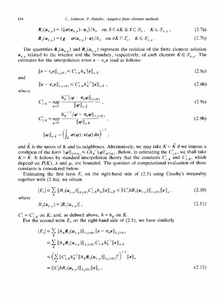
154 C. Johnson, P. Hansbo. Adaptive finite element methods

R2(uh,,,) = :[u(u~.~). n,] lh, on S C dK if S E Y, , K E Yh ,, , (2.7a)

R&J = (g - 4uh.J. 4 lh, on X n &, K E &+ . (2.7b)

The quantities R,(u,,,,,) and R,(u,.,) represent the residual of the finite element solution

‘h.p related to the interior and the boundary, respectively, of each element K E Yh,P. The estimates for the interpolation error e - rrhe read as follows:

Ile - 71,41L2W) d ~I.K~Kll~llU.17 (2.8a)

) d GKG%ll,., 7 (2.8b)

and

Ile - vlIL2(aK where

h,’ c; K = sup

._ lb - ~h~IIL(K)

cpE” (2.9a)

(2.9b)

and k is the union of K and its neighbours. Alternatively, we may take K = k if we impose a condi$on of the form JJ~pJJH~~Kj d Ch,’ JJ+DPJI~~(~). Below, in estimating the Ci..i, we shall take K = K. It follows by standard interpolation theory that the constants Cl;,, and Ci,K, which depend on P(K), A and p, are bounded. The question of computational evaluation of these constants is considered below.

Estimating the first term E, on the right-hand side of (2.5) using Cauchy’s inequality together with (2.8a), we obtain

I’%( d 2 ilR,(uh.,)ii K

L~~K~C;.K~K~~~~,,~ d ~~C’;h~,(~h,,)~l,~~,,~~e~~. 7 (2.10)

where

R,(uh.,>) = k(%,)I 9

Cl = Cl,, on K, and, as defined above, h = h, on K. For the second term E, on the right-hand side of (2.5), we have similarly

(2.11)

lE,l d T (lhKRZ(llh.p)l(LZ(?rK)lle - “heiiL2(ilK)

sc IlhKR2(Uh,p)llLZ(iiK~C:,Kh~211ellil.K K

(2.12)

C. Johnson, P. Hansbo, Adaptive finite element methods

where C; = Ck K on K,

155

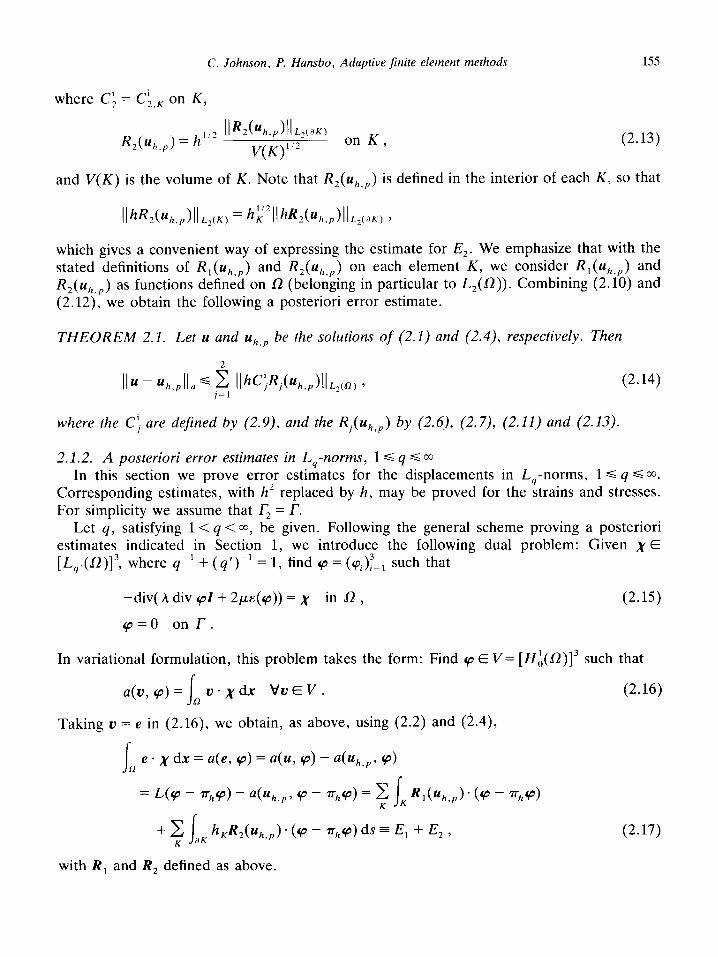
R2(u,,,) = Q/2 ““2y;\;*(JK) on K, (2.13)

and V(K) is the volume of K. Note that R,(u,,,) is defined in the interior of each K, so that

lI~~2(%,,)IIL2(K) = h~211hR2(u,,,)llLz(aK) 3

which gives a convenient way of expressing the estimate for E,. We emphasize that with the stated definitions of R,(u,,,) and R,(u,,,) on each element K, we consider R,(u,,,) and R,(u,,,) as functions defined on a (belonging in particular to L2(0)). Combining (2.10) and (2.12), we obtain the following a posteriori error estimate.

THEOREM 2.1. Let u and u~,~ be the solutions of (2.1) and (2.4), respectively. Then

lb - %,Ja y$ IlhC~.Ri(~,,,)II,Z(a) ’ (2.14)

where the C; are defined by (2.9), and the Rj(u,,,) by (2.6), (2.7), (2.11) and (2.13).

2.1.2. A posteriori error estimates in L4-norms, 1 d q d ~0 In this section we prove error estimates for the displacements in L,-norms, 1 d q s ~0.

Corresponding estimates, with h2 replaced by h, may be proved for the strains and stresses. For simplicity we assume that r2 = K

Let q, satisfying 1 < q < ~0, be given. Following the general scheme proving a posteriori estimates indicated in Section 1, we introduce the following dual problem: Given x E [L,,(n)]“, where 4-l + (q’)-1 = 1, find cp = (cp,);_, such that

-div( h div qpZ + 2&p)) = x in 0 , (2.15)

q=O onr.

In variational formulation, this problem takes the form: Find 4p E V= [HA(n)]” such that

a@, 9) = I n u.Xdx VuEV. (2.16)

Taking u = e in (2.16), we obtain, as above, using (2.2) and (i.4),

+C hKR,(u,.,) * b - w’) ds = E, + E, 7 K

(2.17)

with R, and R, defined as above.


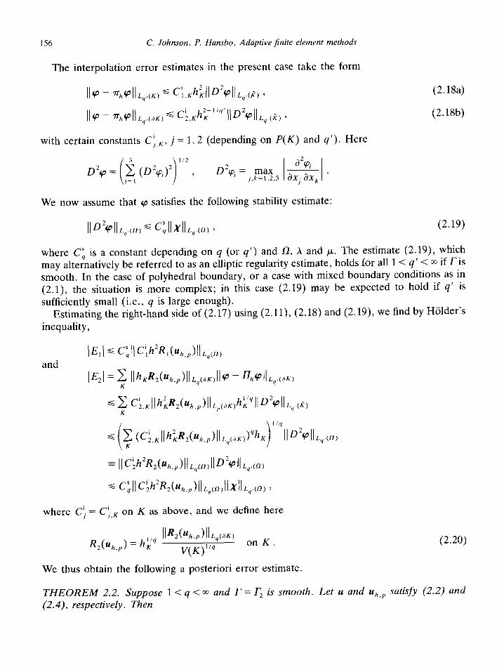
The interpolation error estimates in the present case take the form

(2.18a)

(2.18b)

with certain constants C:. K, j = 1,2 (depending on P(K) and s ‘) . Here

We now assume that 9 satisfies the following stability estimate:

Il~*44L,.(n) d C;llxllL,in, ’ (2.19)

where Ci is a constant depending on q (or q’) and 0, h and /_L The estimate (2.19), which may alternatively be referred to as an elliptic regularity estimate, holds for all 1 < q’ < ~0 if ris smooth. In the case of polyhedral boundary, or a case with mixed boundary conditions as in (2.1), the situation is more complex; in this case (2.19) may be expected to hold if q’ is

sufficiently small (i.e., q is large enough). Estimating the right-hand side of (2.17) using (2.11), (2.18) and (2.19), we find by Holder’s

inequality,

and

i i

l/q

d c (C;,KIlhZ,R2(Uh,,)llL4(aK))qhK llD2~llLq,(f) K

where Cf = Ci,K on K as above, and we define here

M%.,) = cq II~2(%p)llLq(dK)

V(K)“’ on K. (2.20)

We thus obtain the following a posteriori error estimate.

THEOREM 2.2. Suppose 1 < q < 0~ and r = IJ, is smooth. Let u and u~,~ satisfy (2.2) and (2.4), respectively. Then


with the R, de~ned by (2.61, (2.71, (2.11) and (2.201, the Ci are the interrogation co~tants in (2.18) and CS, is the stability constant in (2.19).

REMARK 2.1. It is possible to prove (2.21) with 4 = a if we choose

C”, = c:llog h,;“( ,

where CL is a constant depending on fz, h and /J, and where hmin = min, h. This estimate in particular applies to the case of a general polyhedral boundary including also mixed boundary conditions.

REMARK 2.2. Estimates of the stresses or strains of the form

may be proved by similar techniques. In the case of a non-convex polyhedral boundary, or problems with mixed boundary conditions, one can prove weighted norm analogs of (2.21), of particular interest in the case where q is not large (e.g., in the case q = 2) taking so called pollution effects into account.

REPARK 2.3. In the case of a piecewise linear approximation on tetrahedrons (p = l), we will have R1(u,,,) =J If f is smooth we can, in this case, replace the RI-terms in (2.14) and

(2.21) by llh3C#&Z(nj and llh4C;@&,q(nj’ respectively, with suitably modified interpola-

tion constants C;. This effectively means that in the case of a piecewise linear approximation and a smooth f, the RI-terms in the a posteriori error estimate may be neglected (cf. Section

5).

2.2. Adaptive algorithms, reliability and ejjkiency

As indicated, starting from an a posteriori error estimate such as (2.21) or (2.14), we may design adaptive algorithms based on seeking a mesh $iy;pt with (nearly) as few degrees of freedom as possible, such that

(2.22)

This is a non-linear minimization problem which may be solved approximately in an iterative process, seeking to equidistribute the element contributions in the sum over the elements in the definition of CT_, l~h2C:Ri(U,,,)/1L,ta, (see [2,11)). For instance, in the case q = =J, with

the indicated dependence of CS, on log(h,i’,), the corresponding adaptive algorithm based on (2.22) would take the following form if p is constant: Given a mesh TfiOld with mesh size hoId


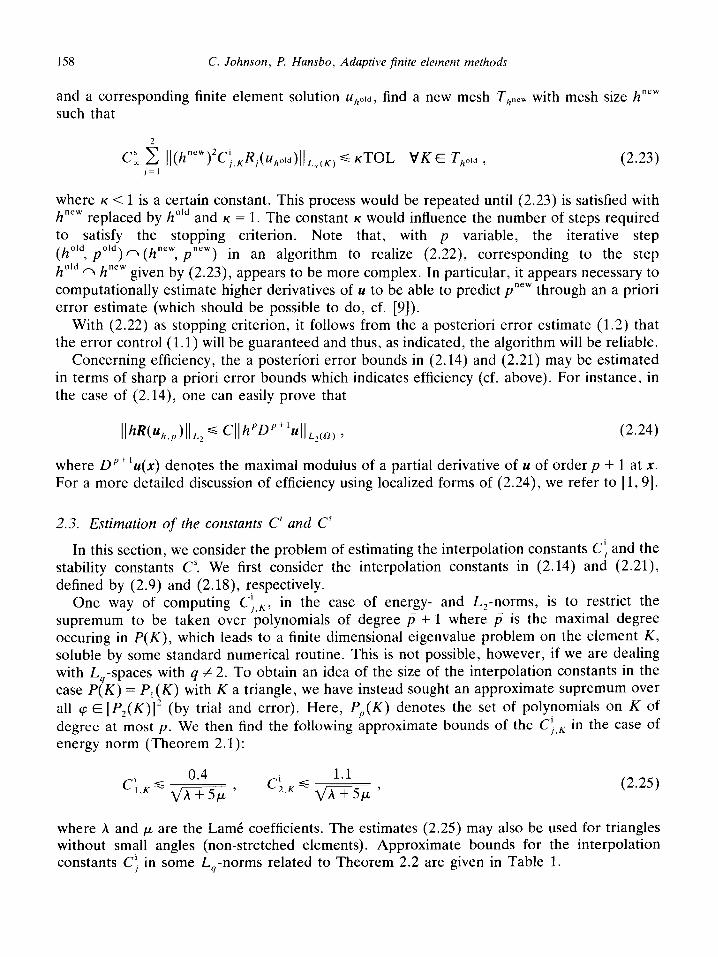
and a corresponding finite element solution uhold, find a new mesh T,,,,, with mesh size h”“” such that

(2.23)

where K < 1 is a certain constant. This process would be repeated until (2.23) is satisfied with h new replaced by hoId and K = 1. The constant K would influence the number of steps required to satisfy the stopping criterion. Note that, with p variable, the iterative step

(;;dk~;;Jwn (h”? p”““) m an algorithm to realize (2.22), corresponding to the step h given by (2.23), appears to be more complex. In particular, it appears necessary to computationally estimate higher derivatives of u to be able to predict p”“” through an a priori error estimate (which should be possible to do, cf. [9]).

With (2.22) as stopping criterion, it follows from the a posteriori error estimate (1.2) that the error control (1.1) will be guaranteed and thus, as indicated, the algorithm will be reliable.

Concerning efficiency, the a posteriori error bounds in (2.14) and (2.21) may be estimated in terms of sharp a priori error bounds which indicates efficiency (cf. above). For instance, in the case of (2.14), one can easily prove that

(2.24)

where Dp+’ u(x) denotes the maximal modulus of a partial derivative of u of order p + 1 at X. For a more detailed discussion of efficiency using localized forms of (2.24), we refer to [l, 91.

2.3. Estimation of the constants C’ and C”

In this section, we consider the problem of estimating the interpolation constants Cf and the stability constants C’. We first consider the interpolation constants in (2.14) and (2.21), defined by (2.9) and (2.18), respectively.

One way of computing C;,,, in the case of energy- and &-norms, is to restrict the supremum to be taken over polynomials of degree p + 1 where ~7 is the maximal degree occuring in P(K), which leads to a finite dimensional eigenvalue problem on the element K, soluble by some standard numerical routine. This is not possible, however, if we are dealing with L,-spaces with 4 # 2. To obtain an idea of the size of the interpolation constants in the case P(K) = P,(K) with K a triangle, we have instead sought an approximate supremum over all cp E [P,(K)]* (by trial and error). Here, P,(K) denotes the set of polynomials on K of degree at most p. We then find the following approximate bounds of the C), in the case of energy norm (Theorem 2.1):

(2.25)

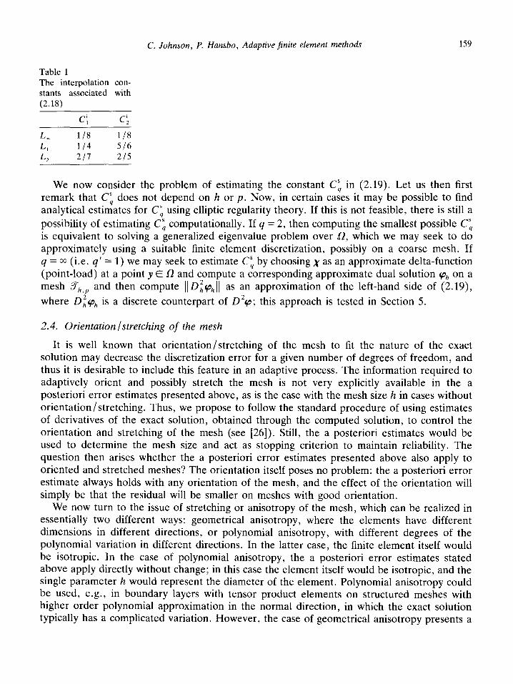
where A and p are the Lame coefficients. The estimates (2.25) may also be used for triangles without small angles (non-stretched elements). Approximate bounds for the interpolation constants C) in some L,-norms related to Theorem 2.2 are given in Table 1.


Table 1 The interpolation constants associated with (2.18)

C’, G L l/8 118 L, l/4 516

L* 217 215

We now consider the problem of estimating the constant Cb in (2.19). Let us then first remark that Ci does not depend on h or p. Now, in certain cases it may be possible to find analytical estimates for Ci using elliptic regularity theory. If this is not feasible, there is still a possibility of estimating Ci computationally. If 9 = 2, then computing the smallest possible CS, is equivalent to solving a generalized eigenvalue problem over 0, which we may seek to do approximately using a suitable finite element discretization, possibly on a coarse mesh. If 4 = ~0 (i.e. 9’ = 1) we may seek to estimate Ci by choosing x as an approximate delta-function (point-load) at a point y E J2 and compute a corresponding approximate dual solution qh on a mesh Th p and then compute I[D~v~[I as an approximation of the left-hand side of (2.19),

where D;fqh is a discrete counterpart of D24p; this approach is tested in Section 5.

2.4. Orientation /stretching of the mesh

It is well known that orientation/stretching of the mesh to fit the nature of the exact solution may decrease the discretization error for a given number of degrees of freedom, and thus it is desirable to include this feature in an adaptive process. The information required to adaptively orient and possibly stretch the mesh is not very explicitly available in the a posteriori error estimates presented above, as is the case with the mesh size h in cases without orientation/stretching. Thus, we propose to follow the standard procedure of using estimates of derivatives of the exact solution, obtained through the computed solution, to control the orientation and stretching of the mesh (see [26]). Still, the a posteriori estimates would be used to determine the mesh size and act as stopping criterion to maintain reliability. The question then arises whether the a posteriori error estimates presented above also apply to oriented and stretched meshes? The orientation itself poses no problem: the a posteriori error estimate always holds with any orientation of the mesh, and the effect of the orientation will simply be that the residual will be smaller on meshes with good orientation.

We now turn to the issue of stretching or anisotropy of the mesh, which can be realized in essentially two different ways: geometrical anisotropy, where the elements have different dimensions in different directions, or polynomial anisotropy, with different degrees of the polynomial variation in different directions. In the latter case, the finite element itself would be isotropic. In the case of polynomial anisotropy, the a posteriori error estimates stated above apply directly without change; in this case the element itself would be isotropic, and the single parameter h would represent the diameter of the element. Polynomial anisotropy could be used, e.g., in boundary layers with tensor product elements on structured meshes with higher order polynomial approximation in the normal direction, in which the exact solution typically has a complicated variation. However, the case of geometrical anisotropy presents a

problem for the a posteriori error estimates above, since these estimates, as stated, cannot take advantage of the different mesh size in different directions.

To indicate how to obtain improved estimates for geometrical anisotropy in the case of structured meshes, let &? be a square in CR,‘, and let Y h,p be a rectangular mesh given by a subdivision {nf) in the x,-direction and a subdivision {xi} in the x,-direction, with mesh functions h, in X, and hz in x,, and let V, be the corresponding space of continuous piecewise bilinear displacements. Suppose fi, << h, corresponding to a situation where u has a rapid variation in x2 and a slow variation in x1. Let the set of faces (element sides) Y,, be divided into the set YF1 of the sides perpendicular to the x,-axis and the set of sides Y,,2 perpendicular to the x2-axes, Assuming r, = r, the representation formula (2.6) now takes the form

Let P, and P2 be the $-projections onto the set of continuous piecewise linear functions on the meshes {x’,} and {xi>, respectively, and define =& = PIP2. Taking into account that the x,-derivatives of finite element displacements have a contin~ous~ piecewise Linear variation in X, , and vice versa, we find the following error representation, using the orthogonaIities for PI and Fz:

and f - f denotes the jump in the indicated quantity. Arguing as above, we now obtain the following variant of the a posteriori error estimate (2.14):

Ilu-u h,Ja g II@* + wt~l(%,p)llL,(n) + Ilh,C:~,,(~,,,)ll,,in)

+ I/h2C:L)2:(“h,p)IlLZ(“) f where on an element K

where we take the maximum over the sides of K pe~endicular to x1 and x*, respectively. The important feature of this estimate is that h, is combined with the jump [L),(u,)] in the

C. Johnson, P. Hanrbo, Adaptive finite element methods 161

x,-direction, where ~~~~~) only contains derivatives with respect to x1 and similarly for x2. We thus have in the jump terms a complete separation in x1 and x,, so that h, is combined with x,-derivatives (which are not large) and h, with x,-derivatives (which are large). This is a necessary feature in order to be able to take advantage of the small mesh size h, in the x,-direction. Here, a combination of h, with an x,-derivative would lead to an inefficient algorithm. Such a combination occurs here in the R, -term, but this occurrence is much less harmful than in the jump terms.

We have briefly indicated how to handle oriented/stretched meshes in the a posteriori error estimates underlying the adaptive algorithms. Here, only geometrical anisotropy poses a problem, which may be resolved on structured tensor-product meshes as indicated. The problem of proving efficient a posteriori error estimates on general meshes with large geometrical anisotropy is open. It appears, however, that such meshes do not occur frequently in practice, since large stretching is usually coupled with structured meshes.

3. Non-linear elliptic problems: small strain elasto-plasticity

3.1. fiencky ‘s problem

As an example of a monotone non-linear elliptic problem, we present in this section an a posteriori error estimate for a finite element method for a Hencky problem in small strain perfect plasticity with the Von Mises yield criterion. Although not adequate as a model for plasticity problems in general, the Hencky model contains the essential theoretical difficulties of the more satisfactory Prandtl-Reuss incremental model; in fact, each step in an incremental formulation of plasticity requires the solution of a Hencky-type problem. Thus, the extension of our results to a small strain incremental formulation poses no additional theoretical or computational difficulties. Numerical results for the Prandtl-Reuss plasticity problem will be reported in future work. The extension to large strain plasticity is a problem of great significance in applications which, again, we hope to return to in later work. It is interesting to note that also in the latter case the Hencky problem plays an important role in an incremental process (see [27]).

The material of this section gives extensions of the results of [13], where a posteriori error estimates for a finite element method for a simpler model problem in plasticity (the antiplane shear problem) were presented.

The Hencky problem in perfect plasticity with the Von Mises yield criterion may be formulated as follows, with the notation of Section 2. Find the displacement u and the stress e such that

0 = K7(2/LLED(U)) + 3A+2,~

3 div 111 in 0 , (3.la)

-divu=f in L?,

u=O onr,

(3Sb)

(3.lc)

where 0 is a bounded domain in R3, rD = 7 - f tr TZ= 7 - $fE~,, T~~)Z is the stress de- viatoric corresponding to T, and


where cY is a material constant and 171 = (7 : T)*“.

To avoid some technical difficulties in the formulation (3.1), associated with the fact that the displacement u may be discontinuous (e.g., corresponding to the presence of slip lines), in which case the meaning of (3.la) is not obvious (cf. [28]) we shall, for convenience, consider the following regularized variant of (3. l), corresponding to a slightly viscous, perfectly plastic material: Given y > 0 small, find (u,, , u,,) E H x V such that

1 - a; +

1

2P 9A+6p tr uYZ + t (a,P - na,“) = E(u,) in 0 , (3.2a)

1 R aY: E(U) dx = f.udx tlvEV, (3.2b)

where V= [H;,(n)]” 2 H = (7 = (T,i)&,: Ti/ = 7/, E L,(R)} .

Note that (3.2) formally tends to (3.1) as y-,0. The regularization is introduced with the sole purpose of simplifying the statement and the proof of the a posteriori error estimate, and the actual value of the regularization parameter y (small) will be insignificant.

Let Vh = Vh,P be a finite element space as above and consider the following finite element method: Find (a,,, , u~,~) E H x V, such that

1 - uyi, +

1

2P ’ 9h+6p tr QIZ + t (a;* - fl&) = E(u,,h) in R , (3.3a)

U y,h : tz(u) dx = (3.3b)

In practice, we may take y = 0 in (3.3), since V, C V, which gives the following analog of (3.1), formulated in displacements only: Find uh E V,, such that

~(2wDhJ: 44 dx + I 3h+2/_~ R 3 div uh div u dx = (3.4)

for all u E V,, .

3.2. An a posteriori error estimate for the stresses

We now state and prove an a posteriori error estimate for the stresses in the finite element method (3.3) (or (3.4)) for the Hencky problem (3.1) in the complementary energy norm

corresponding to the energy norm in the linear elasticity problem of Section 2, in the sense that ]Iu(u)]lU~~ = ((u[], if (2.la) holds.

C. Johnson, I? Hunsbo, Adaptive finite element methods 163

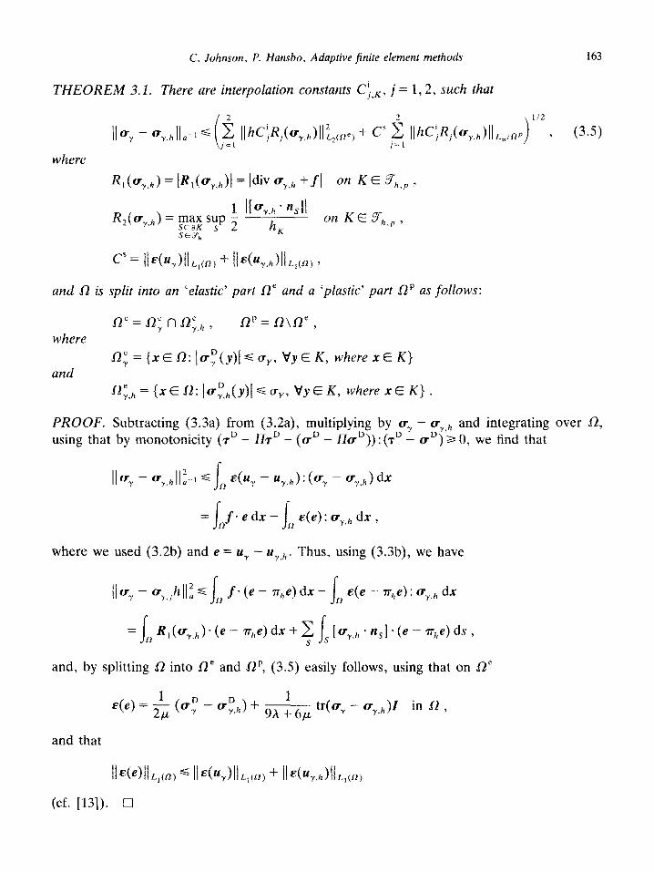
THEOREM 3.1. There are interpolation constants Cl*,: j = 1,2, such that

and R is split into an ‘elastic’ part Lliz’ and a ‘plastic’ part Op as follows:

ne = 0; f-l qh ) i-.lp = n\ne )

where

and 0; = {x E R: lay(y)1 G u,,, Vy E K, where xE K}

‘RG.h = {x E 0: lori,(y)/ G uy, Vy E K, where x E K} .

PROOF. Subtracting (3.3a) from (3.2a), multiplying by a7 - uY,h and integrating over ~2, using that by monotonicity (7D - ZYIkD - (uD - ZIu”)) : (TV - uD) a 0, we find that

where we used (3.2b) and e = u, - u~,~. Thus, using (3.3b), we have

and, by splitting R into 0’ and fl p, (3.5) easily follows, using that on fle

e(e) = $ (u,D - u:,) f 1

9hf6p tr(u, - u~,~)Z in 0 ,

and that

Il44llL,ja) 9 lI4fqIlL,(n) + ll~(+&(n,

(cf. [13]). 0

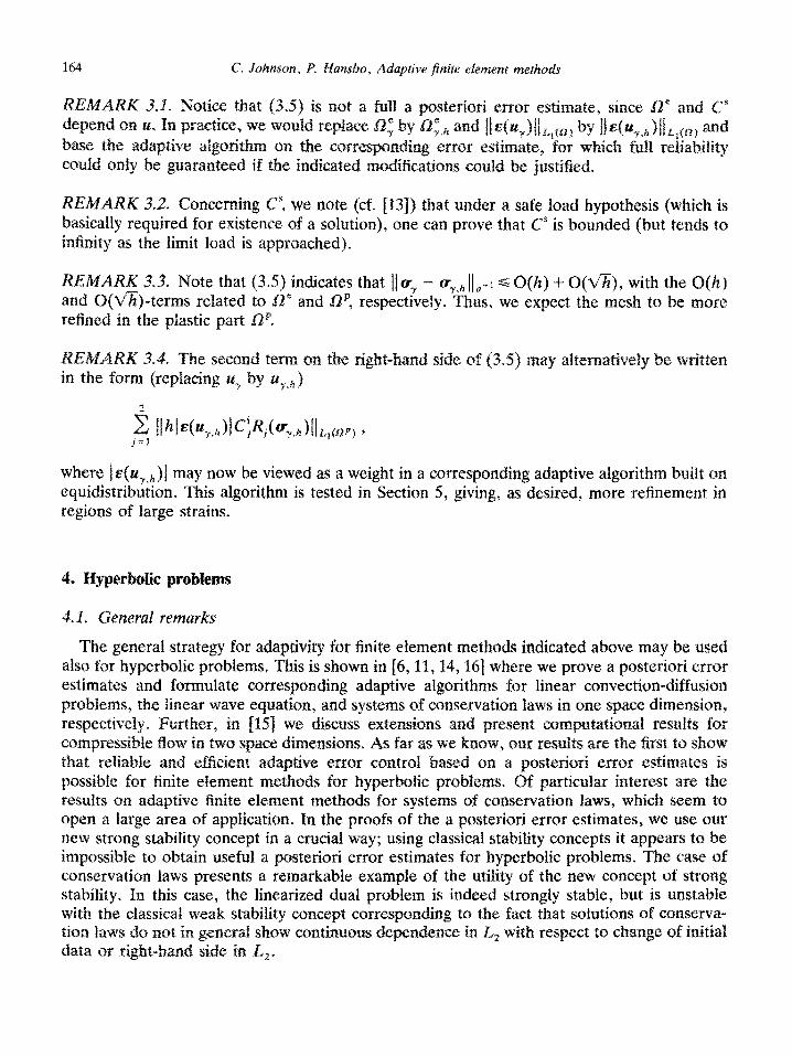
~~~A~~ 3.1. Notice that (3.5) is not a full a psteriori error estimate, since fJ2” and C” depend on tc, In practice, we would replace $2; by fz;,& and ft E(u,)/~.~~~~ by ~~&(~~~*)~~~~~~~ and base the adaptive a~go~thm on the co~~s~ond~ng error estimate, for which f&B re~ab~~~t~ could only be guaranteed if the indicated mod~~cat~ons co&d be justified.

~~~A~~ 3.2. Concerning C”, we note (cf. [133) that under ix safe load hypothesis (which is basically required for existence of a solution), one can prove that C” is bounded (but tends to i~~~~~y as the limit load is a~~~~~~hed).

REiKARK 3.3. Note that (3.5) indicates that lja, - v~,~//~-~ 6 O(h) -i- O(V%), with the Cr;(aZ) and Q(a)-terms related to R” and LP, respectively. Thus, we expect the mesh to be more refined in the pbstic part W,

where j&(~)l may now be viewed as tr weight in a corresponding adaptive algorithm built on equidistribution. This algorithm is tested in Section 5, giving, as desired, more refinement in regions of large strains,

The general strategy for ~da~~~~i~~ for finite element rn~tb~~s indicated above may be used also for hyperbolic problems, This is shown in t&11,14, ‘lrj] where we prove a posteriari error estimates and formulate correspoading adaptive algorithms for linear convection-diffusion problems, the linear wave equation, and systems of conservation laws in one space dimension, respectively. Further, in fl51 we discuss extensions and present ~rn~~tat~ona~ resuhs for co~~~~~b~e f&w in two space d~rn~~s~~~s~ As far as we know, our results are the first to show that reliable and ef~c~~n~ ~da~~ve error control based on a poster-k error es~rn~t~s is possible for finite element methods for hype&ok problems. Qf particular interest are the results on adaptive finite element methads for systems of conservation laws, which seem tea open a large area of application. In the proofs of the a posteriori error estimates, we use our new strong stabiiity concept in a crucial way; using classical stability concepts it appears to be irn~~~sible to obtain useful a ~~$t~~~ri error estimates for b~~~rbolic problems. The c&se of conservation laws presents a remarkable example of the utility of the new concept of strong stability. In this case, the linearized dual problem is indeed strongly stable, but is unstable with the classical weak stability concept corresponding to the fact that solutions of conservation taws do not in generag show eo~t~~uu~~ dependence in Lz with respect to change of initial data or right-hand side in A,.

To illustrate the essential points, we shall in this section indicate the proof of an a posteriori error estimate for a finite element method for a scalar conservation law in our space dimension (Burgers’ equations. For more details and the ~mportaut extension to the case of systems, we refer to f16j.

4.2. An a posteriori error estimate for a finite element method for Burgers’ equation

We consider Burgers’ equation: Find the scalar function U’ = u’(x, t) such that

(4. la)

where u,, E L,(R) has compact support, and E is a small positive constant. For E > 0, this problem is uniquely solvable. As E tends to zero, the solution u’ will converge to a limit u, the entropy solution of the inviscid Burges’ equation corresponding to (4.1) with E = 0. Even if the data u, is smooth, u( * , t) may become discontinuous in finite time, corresponding to the development of shocks. The entropy condition states that at shocks (d~scontinuities), we have u-(x, C) > u+(x, t), where

is the left-hand and right-hand limit, respectively, This means that close to shocks ~~~/~~ may be very large negative (but au”/ax will be bounded above). In such a case, the linearized problem

(4.2a)

obtained by linearizing (4,la) around the solution ~3, (4.2a) by # and integrating with respect to x leads to

is unstable in L,, since muitip~ying

where the right-hand side may be large if ~~~/~~ is large negative, which corresponds to the fact that (4.1) is not contiuuo~s in L, with respect to ~~-perturbations of initial data. This ~rgumeut seems to indicate that a posterior-i error control in L, for approximate solutions of (4.1) would be impossible in the presence of shocks. The remarkable fact is, however, that such an error control is in fact possible to establish, if we use a proper stability concept and

use the Galerkin orthogonality intrinsic in the finite element method, which we now proceed to demonstrate.

The a posteriori error estimate in 1;,, for a finite element method for (4.1) to be presented, may be extended to the case of system of conservation laws in one space dimension. This yields a way out of the stalemate position of the classical approach to conservation laws, based on &-continuity, which is limited to the scalar case.

For simplicity, we shall consider a “semi-discrete’ finite element method for (4.2) of the form of ‘exact transport + &-projection’ (cf. [l?]). The extension to the fully discrete case with space-time elements follows the same principles (see 1161).

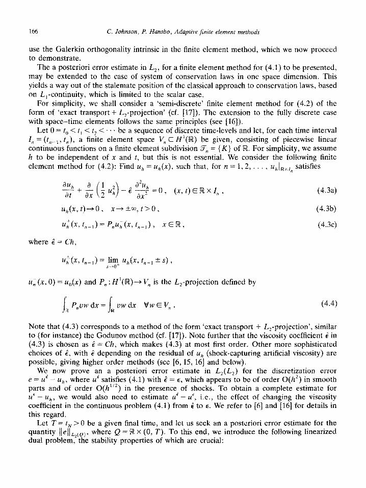
Let 0 = t,, < t, < t, < f - . be a sequence of discrete time-levels and let, for each time interval Z,, = (fn_I, t,>, a finite element space V, C ~I(~~ be given, consisting of piecewise linear continuous functions on a finite element subdivision yfl = (K) of R. For simpticity, we assume h to be independent of x and t, but this is not essential. We consider the following finite element method for (4.2): Find uh = u~(x>, such that, for p1= 1,2, . . . , uhlRx,,, satisfies

au, a 1 at+- -u; c > n a2u,

ax 2 --E.------o, (XJ)ERXZn,

a?

u, (x, 0) = U,(X) and P, : H”(R)-+ V,, is the &-projection defined by

I r% P,vwdx= vwdx VwEV,.

(4.3a)

(4.3b)

(4.3c)

(4.4)

Note that (4.3) corresponds to a method of the form ‘exact transport + &-projection’, similar to (for instance) the Godunov method (cf. [17]). Note further that the viscosity coefficient g in (4,3) is chosen as i = CrZ, which makes (4.3) at most first order. Other more sophisticated choices of i, with Z depending on the residual of uh (shock-capturing artificial viscosity) are possible, giving higher order methods (see [6,15, 161 and below).

We now prove an a posteriori error estimate in II,,,(L,) for the discretization error e=u’-u,, where uQ satisfies (4.1) with 2 = E, which appears to be of order 0(/z’) in smooth parts and of order O(h”*) in the presence of shocks. To obtain a complete estimate for tie - U,&, we would also need to estimate ui - ~8, i.e., the effect of changing the viscosity coefficient in the continuous problem (4.1) from 2 to E. We refer to [B] and 1161 for details in this regard.

Let T = t, > 0 be a given final time, and let us seek an a posteriori error estimate for the

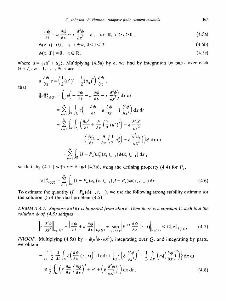
quantity lM,cpt7 where Q = R x (0, T). To this end, we introduce the following Linearized dual probfem, the stability properties of which are crucial:

C. fohnson, P. Nansito, Adaptive finite element ~~eth~d~ IS7

(4Sa)

(4Sb)

c/+, T)=O, XER, (4.5c)

where a = $(u’ + uh). Multiplying (4Sa) by e, we find by integration by parts over each R X l,, n. = 1, . _ . , N, since

so that, by (4.la) with E = 2 and (4.3a), using the defining property (4.4) for P,,

To estimate the quantity (I- P,)qb(* , tlP_l), we use the following strong stability estimate for the solution # of the dual problem (4.5).

PROOF, Multiplying (4.5a) by -<(a’#/ax*), integrating over Q, and integrating by parts, we obtain

integrates to zero. 17

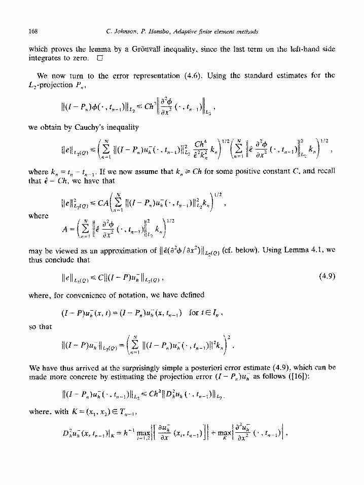
We now turn to the error representation ~~~~r~j~ctio~ P,,

(4.6). Using t,he standard estimates for the

where k, = t,z - b,_, . If we naw assume that k, 2 Ch for some positive constant C, and recall that $2 = C!z, we have that

may be viewed as an a~~r~xirna~~on of f]2(&$ /&x’)/\ La(Q) {ccf, below). Using Lemma 4. I I we

thus conclude that

(4.9)

where, for convenience of notation, we have defined

We have thus arrived at the ~~~~r~singly simple a posteriori error estimate (4.9), which can be made more concrete by estimating the projection error (I - P),t)~i as foIlows ([14]):


with [(~u,/&)(x~, t,_r)] the jump in the derivative au,/& at (xi, t,_r). Extending D2u, to (0, T) by defining

Diui(x, t) = D2u,(x, t,_I) for t E Z, ,

we can thus express the a posteriori error estimate (4.6) alternatively as follows:

(4.10)

Some comments are in order. First, the assumption used above, that A = II l (a24 /~~~)ll,~(~), can easily to avoided, using the presence of the other terms in the strong stability estimate (4.5) (see [16] for details). Secondly, the a posteriori estimate (4.10) appears to be optimal, i.e., in particular second order accurate for smooth solutions. This is a consequence of the choice of i as i = Ch, which itself would correspond to an O(h) perturbation for smooth solutions, and thus reduce the accuracy of the total approximation to first order. With the more elaborate choice of E as, for instance < = C max(h2R(u,), h3’2), where Z?(U~) is the residual of uh defined below, which is a typical choice of the artificial viscosity in the shock capturing streamline diffusion method (see [6, 15,16]), we would obtain a method of total accuracy 0(h3’2) for smooth solutions satisfying the following a posteriori error estimate (cf. (1.5)):

or llell Lz(Q) d ‘11 min(1, h1’2R(U,))(),2(Q, , (4.11)

lkll L*(Q) d ciI min(1, h3’2D2Uk)(lL2(Q) 7 (4.12)

where we define R(u,,) = (I- P,)u,(- , t,_I)/h on Z,. We summarize the results obtained for Burgers’ equation as follows where the assumption

of boundedness of up and u,, is used in the complete proof in [16].

THEOREM 4.2. Let u,, be the solution of (4.3) and u’ that of (4.1) with E = Z = Ch and k, 2 ch. Suppose that b/ax = $(a /ax)(u’ + uh) is bounded from above, and that up and uh are bounded. Then there are constants C such that

11” - ‘&Q) d ‘il(‘- ‘hii h2(Q) 4 Cilh2D2U, hz(Q) ’ (4.13)

REMARK 4.1. Note that the estimates (4.13) indicate O(a) accuracy (which is optimal) in the presence of shocks, since, in an O(h)-neighbourhood of the shock, the integrands on the right-hand side would be of order 0( 1).

REMARK 4.2. The dual problem (4.5) may be L,-unstable, since multipliction of (4.5a) by 4 gives

= 2 iwax I d" ~J'(x, t) dx + ]R e(x, t)+(x, t) dx ,

170 C. Johnson, P. Hunsbo, Adaptive finite element methods

which may Iead to instabiIity if &r/ax is large negative (cf. the discussion above for the linearized problem (4.2)).

For analogs of 14.13) for full discretizations of (4.1) and extensions to systems of conservation laws in one space dimension, we refer to [ 161, where we also consider the case of rarefaction waves with da/& possibly large for t small (~~/~~ s C/t), using a weighted norm technique. The a posteriori error estimate of Theorem 4.2 may be extended to systems of conservation laws in one dimension under appropriate assumptions including the presence of shocks, contact discontinuities and rarefaction waves. As far as we know, these results are the first to show that a posteriori error control for systems of conservation laws is possible. To establish the crucial stability estimates in the system case correspunding to Lemma 4.1, dia~onalization together with a weighted norm technique is used.

The techniques for proving a posteriori error estimates for conservation laws indicated above may be formally extended to systems of conservation laws in several dimensions, leading to a posteriori error estimates of, e.g., the form (lS), if the corresponding linearized dual problem statisfies strong stability estimates analogous to (4.7). In [15]. we give computational results for the corresponding adaptive algorithms in the case of time-dependent compressible flow in two dimensions. Below, we present a corresponding result for a stationary shock reflection problem. The question of whether the linearized dual problem statisfles the strong stability estimates in the case of systems of conservation laws (or the incompressible Navier-Stokes equations) in several dimensions is theoreticaliy very complex, but, as indicated, may probably be tested com~utationally. We pian to give more details on this topic in future work.

5. Cornputationat resufts

In this section we give some computational results for the model problems discussed in the previous sections. We restrict ourselves to problems in R2 with a piecewise linear approximation on triangles. The interpolation constants Cy used were those given in Section 2.3.

5. I. Lima P e~~~t~~~~~

For simplicity we write, in two Dimensions, u = DE and E = Go; where c and E are now defined as column vectors, i.e., E = [E!~, +, &12 + ~~,j~ and CT = [cr,,, crZ2, LT!.J~, and where

r

I and G =

L

-A

WA + P> A+~/.L

~P(A + P) 0

0

0 7

1

lu 1 corresponding to plane strain conditions, The case of plane stress is covered by replacing A by A in D and G, where A = 2Ap /( A + 2~).


5.1 .l. Validation problem: the unit square In order to obtain a problem with known exact solution, consider (2.1) on the unit square

(0,l) x (0,l) with u = 0 on the boundary and with

f=[ (A + /-a1 -2x,)(1 - 2%)

-2/.LX,(l - X2) - 2( A -t 2&(1 - X1) 1 ’ corresponding to the exact solution

[

0 U=

-x&l - X,)(1 - X2) I ’

The energy norm corresponding to the solution is

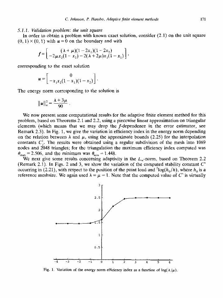
We now present some computational results for the adaptive finite element method for this problem, based on Theorems 2.1 and 2.2, using a piecewise linear approximation on triangular elements (which means that we may drop the f-dependence in the error estimator, see Remark 2.3). In Fig. 1, we give the variation in efficiency index in the energy norm depending on the relation between A and p, using the approximate bounds (2.25) for the interpolation constants Ci. The results were obtained using a regular subdivision of the mesh into 1089 nodes and 2048 triangles; for the triangulation the maximum efficiency index computed was 8 max = 2.506, and the minimum was (9min = 1.448.

We next give some results concerning adaptivity in the L--norm, based on Theorem 2.2 (Remark 2.1). In Figs. 2 and 3, we show the variation of the computed stability constant C” occurring in (2.21), with respect to the position of the point load and 210g(h,/h), where h, is a reference meshsize. We again used A = p = 1. Note that the computed value of C” is virtually

.

1 -

0.5 -

I

-4 -3 -2 -1 0 1 2 3 4 5 6

Fig. 1. Variation of the energy norm efficiency index as a function of log( X /p).

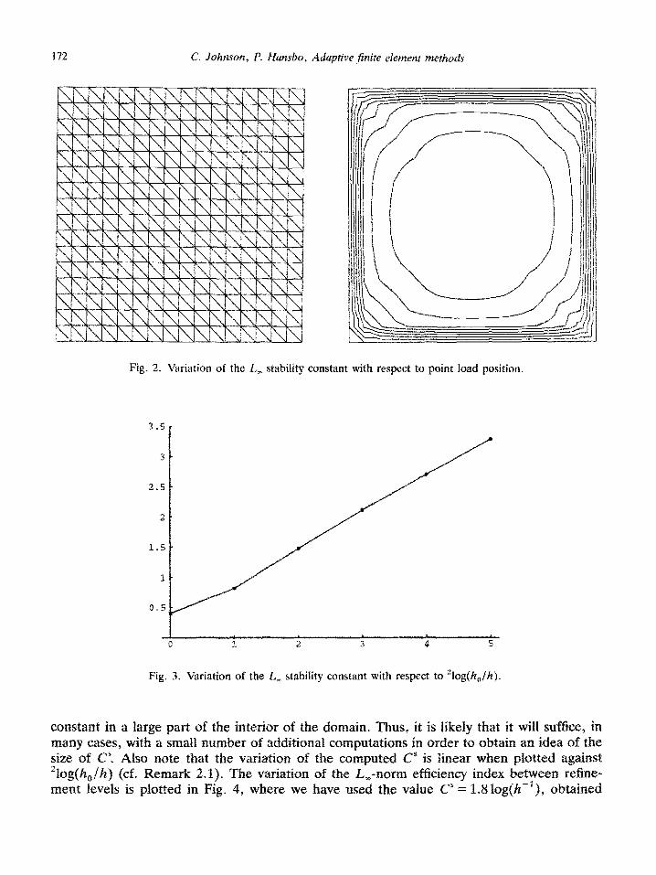
Fig. 2. Variation of the t, stability constant with respect to point load position.

0 z 2 3 4 5

Fig. 3. Variation of the L, stability constant with respect to ‘log(h,/h).

constant in a large part of the interior of the domain. Thus, it is like& that it will suffice, in many cases, with a smalt number of additional ~~rn~utat~~~s ia order tu obtain an idea af the size of C”. Also note that the variation of the computed C” is tinear when plotted against ‘l~g~~~/~~ (cf_ R emark 2.1). The variatirtn of the L,-norm ~f~~e~~~ index between refinement fevels is pbtted in Fig. 4, where we haye used the value C” = 1.8 lugfh-‘1, ~~t~i~~d

C. Johnson, F. Hansbo, Adaptive finite element methods 173

0 1 2 3 4 5

Fig. 4. Variation of the L, efficiency index between refinement levels, C‘ = 1.8 log h-‘.

1.4 -

1.3 -

1.2 -

1.1.

0 1 2 3 4 5

Fig. 5. Variation of the L, efficiency index between refinement levels, C” = 1.8 log hi’.

from Fig. 3. In this example, we in fact observe quadratic convergence without the factor log(~*/~). Nevertheless, the estimate ]]e]] G Ch2 log(l/h) is known to be sharp (an example concerning Poisson’s equation is given in [29]). The corresponding result using a constant value of C” is shown in Fig. 5.

5.1.2. A short cantilever beam with surface load This example has been utilised by a number of authors (see e.g. [23]), where a close

approximation of the energy norm of the exact solution is given as ]] u]]i = 1.903697. The

174

Cl 1 2 3 4

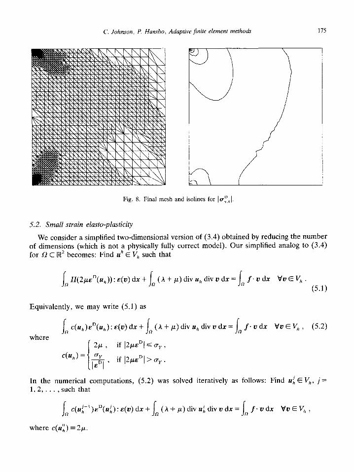
domain is $2 = (0,l) x (0, l), and we assume plane strain conditions, A surface load g = (0, - 1) is applied at x2 = 1 and the beam is clamped along the fine x, = 0, fn Fig. 6, we give the exact energy error ~dasb~d fine) and the a~~ru~~rnate energy error (solid line), The ef~~ie~~~ index increases sIightty from the first to the last level of refinement, from 8 = 1. f to B = 1.3. The mesh and isolines for ~cIK~I {projected onto V,) are shown for the first and final meshes in Figs. 7 and 8,

Fig. 7. First mesh and


Fig. 8. Final mesh and isolines for [a$ I.

5.2. Small strain elasto-plasticity

We consider a simplified two-dimensional version of (3.4) obtained by reducing the number of dimensions (which is not a physically fully correct model). Our simplified analog to (3.4) for R C R2 becomes: Find gh f If;, such that

I n H(~~E~(M~)) : E(U) dx + n (A + p) div u,, div u dx = n f. u dx I I

Vv E V, .

(5.1)

Equivalently, we may write (5.1) as

c(~~)~D(~~):~(~)d~+ VUEV,, (5.2)

where 2Y f

c(qJ = CY

i-

if I2j.k~~~ G uY,

lEDI ’ if 12pEDl > cY .

In the numerical computations, (5.2) was solved iteratively as follows: Find U; E V,, j = 1,2,. . .) such that

where ~(a”,) = 2~.

Further, we used an adaptive a~go~thm based on Theorem 3.2, rnod~~ed according to Remark 3.4 in order to take into account the Iocal variation of the strains.

We consider the unit square, LI = (0,l) X (0, l), submitted to compression. Boundary conditions are given by U, = 0 at x, = 0 and u2 = 0 at x2 = 0 (corresponding to symmetry

+ f +

f + + + f

c -6 f ” f + +

+ + c t f -4 + + -t" +

f f t f t + +t + f +” + + f f

f f t c f f + f -I- f + f f

f f + + t + +

4. t- + t + f

Fig. 9. First mesh (deformed) and plastic ZCXXL

ill- +t- ++ ++ ; + + + + + + -t ++ ++ ++ ++ + + + -I” +

++ ++ ++ ++ +

+ f t + + f + f

+i

+ f + f

f + -I- +

i-t f+ + f i + + + + * t + t”

Fig. IO. First refinement and plastic zone.

Fig. IL Second refinement and plastic zane.

Fig. 12. Third refinement and plastic XOIW.

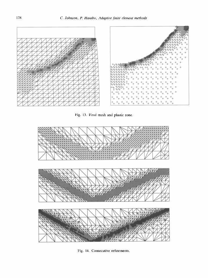
c~~diti~us fur a danain of size (0,2) x (0, Z)), The parameter u-~ = 1; h and g were chosen c~rre~~~~d~~~ to a Ymmg’s ~ud~~~~ of 10’ and a Poismn’s ratio of O-3. 1~ Figs. 9-13, we show the successive meshes and plastic zone fur fq, u2) = (0, -0.0015) units at x2 = 2, and with a tolerance level of 0.002 satisfied on the final mesh,


Fig. 13. Final mesh and plastic zone.

Fig. 14. Consecutive refinements.


Fig. 15. Elevation of the pressure on the final mesh.

5.3. Adaptivity for conservation laws

We show a result for the compressible Euler equations with an adaptive algorithm based on C]]hR{] L2 = TOL (motivated by Theorem 4.2): a stationary shock reflection problem in a domain 4 units long and 1 unit high. The inflow boundary conditions on the right-hand side were set to u = (1.0, 2.9, 0, 5.99) and the inflow conditions on the top of the domain were u = (1.7, 4.45, 0.86, 9.87). We used an explicit, simplified streamline diffusion-type algorithm (corresponding to an O(~)-perturbation of the original problem, in accordance with the analysis in Section 4). Three successive refinements are shown in Fig. 14, and an elevation of the pressure solution in Fig. 15. For further examples concerning Euler’s equations, see [15].

6. Conclusions and prospects for the future

We have briefly outlined a general approach to adaptivity for finite element methods and given concrete applications to some model problems in computational mechanics. The presented methodology appears to have strong potential and opens the possibility of efficient

and reliably ~uant~tat~v~ error control ia a variety of norms for large ciasses of problems of elliptic, parabolic or hyperbolic type* A central component in our approach is the new concept i>f strC?ng stabiMy, which, when Coupled waitir the Galerkin ~~~ugo~a~~t~ inherent in the finite c&merit method, makes it possible to obtain sharp error estimates of both a priori and a posteriori type. The problem of computational evaluation uf the stability properties of the continuous linearized dual problem, connected with the a posteriori error estimates underlying the adaptive algorithms, is fundamental. This problem appears in principle to be possible to salve, even for, e.g., curnp~~~~t~~ flow problems, but more research is required to find cost effective solutions. Other ~rnp~~ta~t topics =cor~err~ a~~or~thrns for adaptive or~e~tat~o~~ stretching of the mesh in space or space-time, which may yield subst~tia~ increase in efficiency, for instance for problems with boundary layers and shocks.

To sum up, the main features of ~dapt~v~~y for finite element methods now seem to be visibfe, and the door is open to ~rnp~ern~~tat~o~ of ada~t~~t~ ia generaf purpose software. A great dea1 of activity in this direction is to be expected over the next few years.

[I] R. Wksson, Adaptive finite clement ~eth~s based on o~~irn~I error estimates for linear efliptZc probfems, Technical Report, Chalmers University of Technology, 15X37.

[Z] K. Eriksson and C. Johnson, Adaptive finite element methods for ~ar~~~~ic probIems f: A linear model ~r~~I~rn~ SIAM .I. Numer. Anal. 28 (I99~) 43-77.

fci] K. Eriksson and C. Johnson, Adaptive fir&e efement methods for parabolic problems If: A priori error ~sti~t~s in L,fL,), TechnicaX Report, Chalmers University of ~~~~o~~y, 1992

{4] IL Eriksson and C. Johnson, Adaptive finite element methods for parabolic problems III: Time steps variable in space and non-coercive problems, Technical Report, Chalmers LJniversity of Technology, 1992.

[S] K. Eriksson and C. Johnson, Adaptive hnite element methods for parabolic problems IV: Non-linear problems, Technical Report, Chalmers University of Technology, 1992.

f6] IL Eriksson and C. Johnson, Adaptive streamline diffusion finite element methods for stationary convcction- diffusion problems, Math. Comg., in press,

!‘7] K. Eriksson and C. Johnson, Adaptive streamline diffusion finite element methods for tim~d~~~~~~~t co~v~ct~on-d~ffns~on problems, to appear*

[g] IL Eriksson and C. Johnson, An adaptive finite element method for linear elliptic Froblems~ Math, Camp. %I (1988) x3-383.

[9] IL Eriksson and C. Johnson, Err5r estimttes and automatic time step controf for ~~~~~n~~~ ~ara~li~ problems, I, SIAM .I. Numer. Anal. 24 (l%G) 12-23.

[XJj C, Johnson, Error estimates and adaptive time step control for a class of one step methods for ~3% ~~~~~~~~

differential equations, SIAM J. Numer, Anal. 25 (1988) 908-926. [ll] C. Johnson, Adaptive finite element methods for diffusion and convection problems, Cornput, Methods Appl,

Mech. Engrg. 82 (1990) 301-322. 1121 C, Johnson, Adaptive finite clement methods for the obsracle problem, Technical Report, Chalmers

University of Technology, Giiteborg, 1991, to appear in M3AAS. [13J 6. Johnson and R Hansbo, Adaptive finite element methods for small strain eI~~f~~la~t~c~ty, I%oc. ~~~A~

Cont. on Finite Inelastic Deformations -Theory and Ap~licat~ons (Urdv. of Hannover, 199%) in press. {I43 C. Sohncron, ~iscont~~uo~~s Gaierkin fItrite element methods for second order h~per~oI~c problems, TcchnicaX

Report, Chalmers Un~~~~~ty of ~echnnlagy, Giiteborg, 1991, to appear in Compnt. Methods Appl. Mech Engrg.


[16] C. Johnson and A. Szepessy, Adaptive streamline diffusion methods for conservation laws, to appear. [17] C. Johnson, A new approach to algorithms for convection problems which are based on exact transport +

projection, Comput. Methods Appl. Mech. Engrg. 100 (1992) 45-62. [18] I. Babuska and W.C. Rheinboldt, A posteriori error estimators for the finite element method, Internat. J.

Numer. Methods Engrg. 12 (1978) 1597-1615. [19] I. Babuska, Feedback, adaptivity and a posteriori estimates in finite elements: Aims, theory, and experience,

in: I. BabuSka et al., eds., Accuracy Estimates and Adaptive Refinements in Finite Element Computations (Wiley, New York, 1986) 3-23.

[20] R. Bank and A. Weiser, Some a posteriori error estimators for elliptic partial differential equations, Math. Comp. 44 (1985) 283-301.

[21] J.T. Oden, L. Demkowicz, W. Rachowicz and T.A. Westermann, Toward a universal h-p adaptive finite element strategy, Part 2. A posteriori error estimation, Comput. Methods Appl. Mech. Engrg. 77 (1989) 113-180.

[22] O.C. Zienkiewicz and J.Z. Zhu, A simple error estimator and adaptive procedure for practical engineering analysis, Internat. J. Numer. Methods Engrg. 24 (1987) 337-357.

[23] M. Ainsworth, J.Z. Zhu, A.W. Craig and O.C. Zienkiewicz, Analysis of the Zienkiewicz-Zhu a posteriori error estimator in the finite element method, Internat. J. Numer. Methods Engrg. 28 (1989) 2161-2174.

[24] R. Verfiirth, A posteriori error estimators for the Stokes equation, Numer. Math. 55 (1989) 309-325. [25] E. Rank and O.C. Zienkiewicz, A simple error estimator in the finite element method, Comm. Appl. Numer.

Methods 3 (1987) 243-249. [26] J. Peraire, M. Vahdati, K. Morgan and 0-C. Zienkiewicz, Adaptive remeshing for compressible flow

computations, J. Comput. Phys. 72 (1987) 449-466. [27] J.C. Simo, A framework for finite strain elastoplasticity based on maximum plastic dissipation and the

multiplicative decomposition. Part II: Computational aspects, Comput. Methods Appl. Mech. Engrg. 68 (1988) 1-31.

[28] R. Temam, Mathematical problems in plasticity (Gauthier-Villars, Paris, 1985). [29] D. Jespersen, Ritz-Galerkin methods for singular boundary value problems, SIAM J. Numer. Anal. 15 (1978)

813-834.

Date post:	06-Feb-2018
Category:	Documents
Upload:	vanxuyen
View:	227 times
Download:	2 times

Adaptive finite element methods in computational mechanicsjjan/transfer/adaptive_hansbo.pdf ·...

Documents