Adaptive Higher-Order Finite Element Methods

for Transient PDE Problems Based on Embedded

Higher-Order Implicit Runge-Kutta Methods

Pavel Solina,b, Lukas Korousc

aDepartment of Mathematics and Statistics, University of Nevada, Reno, USAbInstitute of Thermomechanics, Academy of Sciences of the Czech Republic, Prague

cCharles University, Prague, Czech Republic

Abstract

We present a new class of adaptivity algorithms for time-dependent partialdifferential equations (PDE) that combines adaptive higher-order finite ele-ments (hp-FEM) in space with arbitrary (embedded, higher-order, implicit)Runge-Kutta methods in time. Weak formulation is only created for thestationary residual of the equation, and the Runge-Kutta method is suppliedvia its Butcher’s table. Around 30 Butcher’s tables for various Runge-Kuttamethods with numerically verified orders of local and global truncation errorsare provided. New time-dependent benchmark problem with known exactsolution that contains a moving front of arbitrary steepness is introduced,and used to compare the quality of seven embedded implicit higher-orderRunge-Kutta methods. Numerical experiments also include a comparison ofadaptive low-order FEM and hp-FEM with dynamically changing meshes.All numerical results presented in this paper are easily reproducible in theFEMhub Online Lab (http://femhub.org) and using the Hermes open sourcelibrary (http://hpfem.org/hermes).

Keywords: Runge-Kutta method, Butcher’s table, Finite element method,Automatic adaptivity, Dynamically changing meshes, Reproducible research

Email addresses: solin@unr.edu (Pavel Solin), lukas.korous@gmail.com (LukasKorous)

Preprint submitted to J. Comput. Appl. Math. July 26, 2011

1. Introduction

In recent years, adaptive higher-order spatial discretizations includingspectral elements (SEM), higher-order finite elements (hp-FEM), and higher-order Discontinuous Galerkin (hp-DG) methods have become very popularin computational engineering and science. See, e.g., [6, 10, 12, 14, 17, 22, 23]and the references therein (this list is largely incomplete).

The next task of great practical importance is to combine these techniqueswith adaptive implicit higher-order time integration methods to design robusthigher-order methods for transient problems that are adaptive both in spaceand in time. To our best knowledge, this has not been done yet.

When spatially-adaptive algorithms are extended to transient problems,it is customary to speak about adaptivity with dynamic or dynamically-changing meshes. Mostly this is done with low-order methods both in spaceand in time [1, 2, 9, 15, 16, 18, 19, 24]. Sometimes these methods are wronglyreferred to as ”Space-Time Finite Element Discretizations”, which createsan impression that a d+ 1 dimensional space-time continuum is meshed anddiscretized using d+ 1 dimensional finite elements.

Higher-order spatial discretizations with dynamically-changing meshesare far less frequent in the context of transient problems, and to our bestknowledge they have been only combined with non-adaptive time discretiza-tions or with adaptive lower-order implicit time stepping methods such as in[7, 21].

1.1. Need for Implicit Higher-Order Methods

Explicit time stepping is not practical in conjunction with spatial adap-tivity. This can be seen on parabolic problems where for stability reasonsthe time step size ∆t is limited by the square of the size of the smallest meshelement O(∆h2). This is a serious constraint even without spatial adaptiv-ity. When ∆h is further reduced by mesh refinements, the time step easilybecomes prohibitively small. CFL-like conditions for hyperbolic problemsusually limit the time step by O(∆h) instead of O(∆h2) but the outcome issimilar.

We are particularly interested in embedded implicit higher-order Runge-Kutta methods that provide at the end of each time step a pair of approxi-mations with different orders of accuracy. The difference between these twoapproximations can be used as an a-posteriori error estimator. With sucherror estimator in hand, it is possible to design trivial algorithms for adaptive

2

time step control. These algorithms will not be discussed in this paper, butwe will look at the quality of the error estimate provided by several embeddedimplicit higher-order Runge-Kutta methods.

1.2. Outline

The outline of the paper is as follows: Section 2 provides a brief reviewof Runge-Kutta methods and Butcher’s tables for future reference. Sec-tion 3 explains how the spatial discretization of a transient problem canbe combined with an arbitrary Runge-Kutta method. Section 4 presents adatabase of around 30 Butcher’s tables with verified local and global trunca-tion errors. Section 5 introduces a time-dependent benchmark problem withknown exact solution that contains a moving front of arbitrary steepness.This benchmark is used to compare the quality of seven embedded implicithigher-order Runge-Kutta methods in Section 6. In Section 7 we describe anadaptive algorithm for time-dependent problems with dynamically-changingmeshes that works with any Runge-Kutta method. The algorithm is illus-trated numerically in the same section. Finally, conclusions and outlook areformulated in Section 8.

2. Brief Review of Runge-Kutta Methods

For an ordinary differential equation

dy

dt= f(t, y), (1)

an s-stage Runge-Kutta method has the form

yn+1 = yn + ∆ts∑

j=1

bjkj (2)

where

ki = f

tn + ∆tci, yn + ∆ts∑

j=1

aijkj

. (3)

Here tn is the last time level, ∆t the time step, and aij, bi and ci are knownconstants. The unknowns ki are called stage derivatives and their calcula-tion is the most demanding part of the computation. With known stagederivatives, the new time level approximation yn+1 in (2) is evaluated easily.

3

2.1. Butcher’s Tables

The constants aij, bi and ci in (2), (3) can be written in the form of atable [4],

c1 a11 a12 . . . a1sc2 a21 a22 . . . a2s...

......

...cs as1 as2 . . . ass

b1 b2 . . . bs

Table 1: Butcher’s table of a general Runge-Kutta method.

The Runge-Kutta method is explicit if aij = 0 whenever j ≥ i, diagonallyimplicit if aij = 0 whenever j > i, and fully implicit otherwise. For themoment we will not distinguish between these cases and assume an arbitrarys × s matrix A. However, the final computer code needs to distinguishbetween them for efficiency reasons.

2.2. Embedded Runge-Kutta Methods

A distinct place among Runge-Kutta methods belongs to embedded meth-ods. These methods can be written using a Butcher’s table that has twoB-rows,

c1 a11 a12 . . . a1sc2 a21 a22 . . . a2s...

......

...cs as1 as2 . . . ass

b1 b2 . . . bsb∗1 b∗2 . . . b∗s

.

Table 2: Butcher’s table of an embedded Runge-Kutta method.

The second B-row is used in conjunction with (2) to calculate an extra ap-proximation

y∗n+1 = yn + ∆ts∑

j=1

b∗jkj (4)

4

whose order of accuracy is less than the order of accuracy of the originalapproximation yn+1. Note that the extra approximation y∗n+1 is very cheapsince the stages k1, k2, . . . , ks calculated in (3) are reused without change.

The difference between these two approximations can be used as an a-posteriori error estimator,

en+1 ≈ yn+1 − y∗n+1.

2.3. Butcher’s Tables for Other Than Runge-Kutta Methods

Let us remark that the Butcher’s syntax is not limited to traditionalRunge-Kutta methods. For example, the widely used implicit Crank-Nicolsonmethod has the Butcher’s table

1 1/2 1/20 0 0

1/2 1/2.

2.4. Resources for Runge-Kutta Methods

There is a vast amount of resources on Runge-Kutta methods and Butcher’stables. Many tables and references can be found in the original Butcher’sbook [4]. The Wikipedia page on Runge-Kutta methods [25] contains manyuseful Butcher’s tables and references as well.

3. Application to PDE Problems

Let us consider a general (nonlinear, time-dependent) partial differentialequation

∂u

∂t= f(x1, . . . , xd, t, u,∇u)

that after the semi-discretization is space takes the form

MdY

dt= F (t, Y ). (5)

Here M is the mass matrix, F a (nonlinear) vector-valued function withN components, and Y = Y (t) an N -vector of time-dependent unknown so-lution coefficients. Without time-dependent equation data equation (5) isautonomous, F = F (Y ). Explicit dependence of F on t may come, for ex-ample, from time-dependent equation coefficients, time-dependent boundary

5

conditions, time-dependent forcing term (such as, e.g., heat sources or electricchange density), or time-dependent geometry.

For the application of the Runge-Kutta method (2), (3) we write (5)formally as

dY

dt= M−1F (t, Y ), (6)

although the mass matrix is never inverted in practise.In the light of (6), equations (2) and (3) become

Yn+1 = Yn + ∆ts∑

j=1

bjKj (7)

and

MKi = F

tn + ∆tci, Yn + ∆ts∑

j=1

aijKj

. (8)

3.1. Newton’s Method

Any standard method can be used to solve the nonlinear algebraic sys-tem (8). We will use the Newton’s method as the nonlinearity F usually isdifferentiable. Equation (8) is rewritten as

M 0 . . . 00 M . . . 0...

......

0 0 . . . M

K1

K2...Ks

−F(tn + ∆tc1, Yn + ∆t

∑sj=1 a1jKj

)F(tn + ∆tc2, Yn + ∆t

∑sj=1 a2jKj

)...

F(tn + ∆tcs, Yn + ∆t

∑sj=1 asjKj

)

=

000...0

.(9)

The Ns×Ns Jacobian matrix of the left-hand side has the form

J = Jijsi,j=1

where each Jij is an N ×N matrix of the form

Jij = δijM − aijhJ(tn + ∆tci, Yn + ∆ts∑

j=1

aijKj).

Here J stands for the Jacobian matrix DF (t, Y )/DY , and δij is the Kroneckerdelta.

6

3.2. Efficiency

Clearly, in the finite element method all the nonzero matrices Jij have thesame sparsity structure that, moreover, is identical to the sparsity structureof M . Furthermore, for every i the matrix J(tn + ∆tci, Yn + ∆t

∑sj=1 aijKj)

is the same in all Jij, 1 ≤ j ≤ s. If equation (8) is autonomous, then Jij isthe same for all 1 ≤ i, j ≤ s.

If the time-integration is explicit then the solution of system (8) is re-duced to the solution of s linear algebraic systems with the mass matrix Mon the left-hand side. If the time-integration method is diagonally-implicit(DIRK), then the solution of system (8) is reduced to the solution of s non-linear systems with a N × N Jacobian matrix. The full Ns × Ns Jacobianmatrix should be used only with fully implicit methods whose Butcher’s tablecontains nonzero elements above the diagonal.

4. Database of Verified Butcher’s Tables

After an extensive literature and Internet search we collected around 30Butcher’s tables. Since some tables were incomplete (pending various ”simplecalculations”) and some contained typos, we implemented and tested all ofthem in the FEMhub Online Laboratory [8]. Moreover, for each table weverified numerically the order of local and global truncation errors. Thiswas done for both the lower and higher-order variants in embedded methods.The tables and verification scripts in Python can be found in the publishedworksheet ”Arbitrary RK Method” in the FEMhub Online Lab. To accessit, click on the ”Published Worksheets” button on the login screen.

For illustration let us show two graphs that are part of the publishedworksheet ”Arbitrary RK Method” in the FEMhub Online Lab. They cor-respond to a 5-stage embedded SDIRK method by Cash [5] of orders 2 and4, and show that indeed the orders of the global truncation error are 2 and4, respectively. Note that in the log-log plot, the order of the method isrevealed by the slope of the convergence curve.

7

Figure 1: Log-log plot of the global truncation error for the second-order variant of theembedded implicit SDIRK method by Cash [5].

Figure 2: Log-log plot of the global truncation error for the fourth-order variant of theembedded implicit SDIRK method by Cash [5].

8

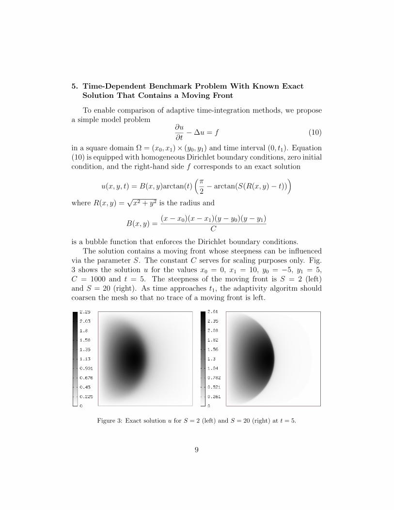
5. Time-Dependent Benchmark Problem With Known ExactSolution That Contains a Moving Front

To enable comparison of adaptive time-integration methods, we proposea simple model problem

∂u

∂t−∆u = f (10)

in a square domain Ω = (x0, x1)× (y0, y1) and time interval (0, t1). Equation(10) is equipped with homogeneous Dirichlet boundary conditions, zero initialcondition, and the right-hand side f corresponds to an exact solution

u(x, y, t) = B(x, y)arctan(t)(π

2− arctan(S(R(x, y)− t))

)where R(x, y) =

√x2 + y2 is the radius and

B(x, y) =(x− x0)(x− x1)(y − y0)(y − y1)

C

is a bubble function that enforces the Dirichlet boundary conditions.The solution contains a moving front whose steepness can be influenced

via the parameter S. The constant C serves for scaling purposes only. Fig.3 shows the solution u for the values x0 = 0, x1 = 10, y0 = −5, y1 = 5,C = 1000 and t = 5. The steepness of the moving front is S = 2 (left)and S = 20 (right). As time approaches t1, the adaptivity algoritm shouldcoarsen the mesh so that no trace of a moving front is left.

Figure 3: Exact solution u for S = 2 (left) and S = 20 (right) at t = 5.

9

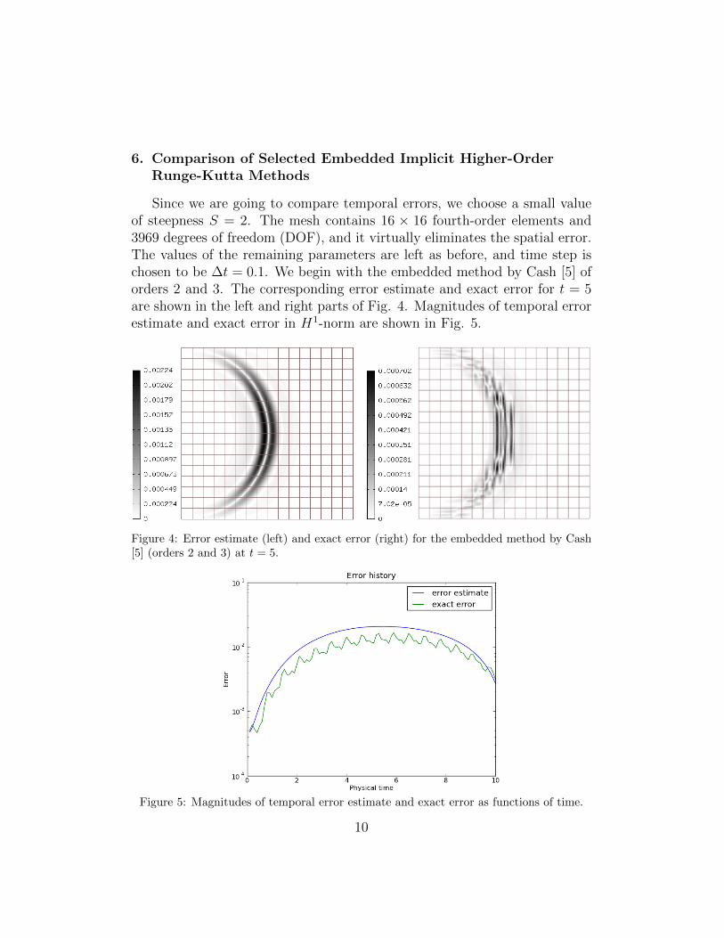
6. Comparison of Selected Embedded Implicit Higher-OrderRunge-Kutta Methods

Since we are going to compare temporal errors, we choose a small valueof steepness S = 2. The mesh contains 16 × 16 fourth-order elements and3969 degrees of freedom (DOF), and it virtually eliminates the spatial error.The values of the remaining parameters are left as before, and time step ischosen to be ∆t = 0.1. We begin with the embedded method by Cash [5] oforders 2 and 3. The corresponding error estimate and exact error for t = 5are shown in the left and right parts of Fig. 4. Magnitudes of temporal errorestimate and exact error in H1-norm are shown in Fig. 5.

Figure 4: Error estimate (left) and exact error (right) for the embedded method by Cash[5] (orders 2 and 3) at t = 5.

Figure 5: Magnitudes of temporal error estimate and exact error as functions of time.

10

Next we consider the embedded method by Billington [3] of orders 2 and3. This method fails. The corresponding error estimate and exact error fort = 5 are shown in the left and right parts of Fig. 6. Magnitudes of temporalerror estimate and exact error are shown in Fig. 7.

Figure 6: Error estimate (left) and exact error (right) for the embedded method by Billing-ton [3] (orders 2 and 3) at t = 5.

Figure 7: Magnitudes of temporal error estimate and exact error as functions of time.

Next let us look at the TR-BDF2 method [11] of orders 2 and 3. Thecorresponding error estimate and exact error for t = 5 are shown in the leftand right parts of Fig. 8. Magnitudes of temporal error estimate and exacterror are shown in Fig. 9.

11

Figure 8: Error estimate (left) and exact error (right) for the embedded method TR-BDF2[11] (orders 2 and 3) at t = 5.

Figure 9: Magnitudes of temporal error estimate and exact error as functions of time.

The next method that we test is TR-X2 [11]. The corresponding errorestimate and exact error for t = 5 are shown in the left and right parts ofFig. 10. Magnitudes of temporal error estimate and exact error are shownin Fig. 11.

12

Figure 10: Error estimate (left) and exact error (right) for the embedded method TR-X2[11] (orders 2 and 3) at t = 5.

Figure 11: Magnitudes of temporal error estimate and exact error as functions of time.

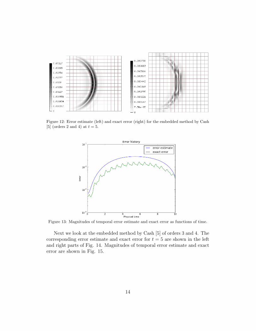
Next on our list is the embedded method by Cash [5] of orders 2 and 4.The corresponding error estimate and exact error for t = 5 are shown in theleft and right parts of Fig. 12. Magnitudes of temporal error estimate andexact error are shown in Fig. 13.

13

Figure 12: Error estimate (left) and exact error (right) for the embedded method by Cash[5] (orders 2 and 4) at t = 5.

Figure 13: Magnitudes of temporal error estimate and exact error as functions of time.

Next we look at the embedded method by Cash [5] of orders 3 and 4. Thecorresponding error estimate and exact error for t = 5 are shown in the leftand right parts of Fig. 14. Magnitudes of temporal error estimate and exacterror are shown in Fig. 15.

14

Figure 14: Error estimate (left) and exact error (right) for the embedded method by Cash[5] (orders 3 and 4) at t = 5.

Figure 15: Magnitudes of temporal error estimate and exact error as functions of time.

The last method on our list is the embedded method by Ismail [13] oforders 4 and 5. The corresponding error estimate and exact error for t = 5are shown in the left and right parts of Fig. 16. Magnitudes of temporalerror estimate and exact error are shown in Fig. 17.

15

Figure 16: Error estimate (left) and exact error (right) for the embedded method by Ismail[13] (orders 4 and 5) at t = 5.

Figure 17: Magnitudes of temporal error estimate and exact error as functions of time.

6.1. Discussion of Results

The reader can see that (with the exception of the Billington’s method) allmethods were capable of identifying correctly the spatial distribution of thetemporal approximation error. The magnitude of the temporal error was bestestimated by the Cash 23, Cash 24 and Cash 34 methods. Remarkably goodresults were obtained by the Cash 34 method. The magnitude of the temporalerror was significantly underestimated by the TR-BDF2, TR-X2 and Ismailmethods. In particular the last is a disappointment since it uses seven stages,and thus it takes lots of CPU time compared to all other methods.

16

7. Spatial Adaptivity with Dynamically-Changing Meshesand Arbitrary Runge-Kutta Methods in Time

Given the limited length of the paper, we have to refer to [7, 20, 21]for basic ideas of multimesh assembling. In particular [7, 21] describe howthe multimesh assembling is used to construct adaptive hp-FEM with dy-namically changing meshes for transient PDE problems. However, papers[7, 21] are based on the Rothe’s method where the temporal discretizationis incorporated into the weak formulation. Thus the implementation of eachnew time stepping method means a new weak formulation and new com-puter code. In order to circumvent this problem, the present study employsthe Method of lines which is more flexible in working with time steppingmethods.

Let us assume that we just finished nth time step and have a locallyrefined mesh τn that was obtained using automatic hp-adaptivity, and anapproximation un on it. The adaptivity algorithm for the next time step isas follows:

Step 1 (Global mesh derefinement):Each time step with the exception of the first one begins with a global meshderefinement. This step is implementation-dependent, and thus let us presentthree options that are available in the Hermes library:

• Reset the mesh τn to a very coarse base mesh τbase. Reset the polyno-mial degrees of all elements to the initial polynomial degree pinit.

• Remove m refinement layers uniformly from all elements in the meshτn. Here m is usually one, two or at most three. Reset the polynomialdegrees of all elements to the initial polynomial degree pinit.

• Remove just one refinement layer uniformly from all elements in themesh τn. Decrease the polynomial degrees of all mesh elements by one.

The first option is mathematically cleanest, meaning that the mesh obtainedon the new time level is completely independent from the mesh that was gen-erated during the last time step. The last option is fastest, but the sequenceof dynamical meshes generated in this way may have on average more DOFthan needed. The second option is a compromise. The coarsened mesh isdenoted by τn+1

r where r = 0 is the counter of adaptivity steps. This is theinitial mesh for the adaptive procedure that will lead to the next time level

17

approximation un+1.

Step 2 (Construction of a solution pair):

The mesh τn+1r is refined globally in both h and p [22] and the resulting mesh

is denoted by τn+1r, ref . Problem (8) is solved on the mesh τn+1

r, ref for the stage

vectors Kn+1r, 1 , K

n+1r, 2 , . . . , K

n+1r, s . The stage vectors are combined linearly with

the basis functions on the mesh τn+1r, ref to obtain their equivalents in the finite

element space on the mesh τn+1r, ref . These continuous, piecewise polynomial

functions are denoted by un+1r, K1

, un+1r, K2

, . . . , un+1r, Ks

. We add up these functions,weighted with the coefficients b1, b2, . . . , bs and the time step, to obtain

un+1r, K = ∆t

s∑j=1

bjun+1r, Kj

.

Next, the functionun+1r, ref = un + un+1

r, K

is projected to the mesh τn+10 to extract its lower-order part. Since the ap-

proximations un and un+1r, K are defined on different meshes which, however,

have a common coarse master mesh, the multimesh assembling technique[21] is employed. This is essential, since the multimesh technique ensuresno loss of information during the projection. The result of the projection isdenoted by un+1

r . Hence we have two approximations with different orders ofaccuracy, un+1

r and un+1r, ref .

Step 3 (Mesh adaptation):

With the solution pair un+1r and un+1

r, ref in hand, we perform one step of hp-adaptivity on the mesh τn+1

r [22]. The result of the mesh adaptation step isdenoted by τn+1

r+1 . With this new mesh in hand, we can increase the counterof adaptivity steps r := r+1 and return to Step 1. The adaptivity algorithmis stopped when the norm of the relative error estimate

errr =‖un+1

r,ref − un+1r ‖

‖un+1r,ref‖

in some adaptivity step r is below a given relative error tolerance. Then wedefine un+1 := un+1

r , τn+1 := τn+1r , and proceed to the next time step.

18

7.1. Comparison of low-order h-FEM and hp-FEM with dynamical meshes

The benchmark problem from Section 5 can be used to compare theperformance of adaptive low-order h-FEM and adaptive hp-FEM. We keepthe same parameter values as in Section 5, including the time step ∆t = 0.1and front steepness S = 20. In all cases, a relative error tolerance for spatialadaptivity of 1% is used as a stopping criterion. For this computation weuse the fully implicit fifth-order three-stage Radau IIA method that virtuallyeliminates the temporal error.

Figs. 18 – 20 show approximate solutions and meshes for t = 2.5, t =5.0 and t = 7.5 obtained with adaptive hp-FEM. In the mesh images, thenumbers stand for polynomial degrees. All elements are quadrilaterals. Twocolors within one element mean different directional polynomial degrees.

Figure 18: Approximate solution and mesh, time t = 2.5.

Figure 19: Approximate solution and mesh, time t = 5.0.

19

Figure 20: Approximate solution and mesh, time t = 7.5.

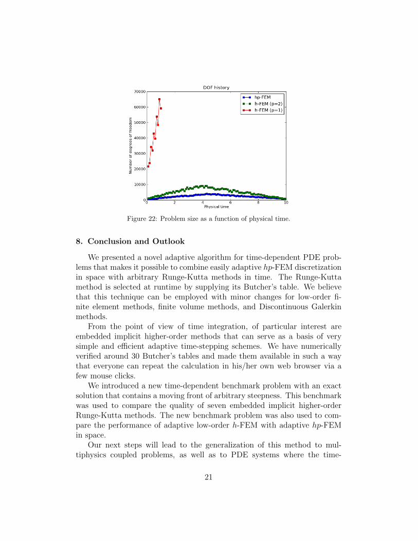
In Fig. 21 we present an analogous result to the hp-FEM mesh shown inthe right part of Fig. 18, but now for adaptive h-FEM with p = 2. While forthe hp-FEM the number of DOF at t = 2.5 was 2637 and for h-FEM withp = 2 it was 6707. For h-FEM with p = 1 the problem size grew rapidly andthe computation was stopped after it exceeded 60000 DOF.

Figure 21: Mesh for adaptive h-FEM with p = 2 at t = 2.5.

A graphical overview of how the number of DOF evolves with physicaltime for these three computations is shown in Fig. 22. The fact that thenumber of DOF is not growing or descending monotonically is due to thestopping criterion. In each time step the adaptivity algorithm stops imme-diately after the error estimate is less than 1%, but the final value can differfrom one time step to another. If the value of the error estimate in step n+1is greater than in step n, then the number of DOF in step n+ 1 can be lesscompared to step n. Whether this happens or not is random.

20

Figure 22: Problem size as a function of physical time.

8. Conclusion and Outlook

We presented a novel adaptive algorithm for time-dependent PDE prob-lems that makes it possible to combine easily adaptive hp-FEM discretizationin space with arbitrary Runge-Kutta methods in time. The Runge-Kuttamethod is selected at runtime by supplying its Butcher’s table. We believethat this technique can be employed with minor changes for low-order fi-nite element methods, finite volume methods, and Discontinuous Galerkinmethods.

From the point of view of time integration, of particular interest areembedded implicit higher-order methods that can serve as a basis of verysimple and efficient adaptive time-stepping schemes. We have numericallyverified around 30 Butcher’s tables and made them available in such a waythat everyone can repeat the calculation in his/her own web browser via afew mouse clicks.

We introduced a new time-dependent benchmark problem with an exactsolution that contains a moving front of arbitrary steepness. This benchmarkwas used to compare the quality of seven embedded implicit higher-orderRunge-Kutta methods. The new benchmark problem was also used to com-pare the performance of adaptive low-order h-FEM with adaptive hp-FEMin space.

Our next steps will lead to the generalization of this method to mul-tiphysics coupled problems, as well as to PDE systems where the time-

21

derivative is not present in all equations (such as in incompressible Navier-Stokes equations).

Acknowledgment

The work of the first author was supported by Subcontract No. 00089911of Battelle Energy Alliance (U.S. Department of Energy intermediary) andby the Grant No. IAA100760702 of the Grant Agency of the Academy ofSciences of the Czech Republic.

References

[1] E. Bansch: An Adaptive Finite-Element Strategy for the Three-Dimensional Time-Dependent Navier-Stokes Equations, J. Com-put. Appl. Math. 36 (1991) 328.

[2] R. Bermejo, J. Carpio: A Space-Time Adaptive Finite Ele-ment Algorithm Based on Dual Weighted Residual Methodologyfor Parabolic Equations. SIAM J. Scientific Computing (2009),3324 3355.

[3] S.R. Billington, Type-Insensitive Codes for the Solution of Stiffand Nonstiff Systems of Ordinary Differential Equations. In: Mas-ter Thesis, University of Manchester, United Kingdom (1983).

[4] J.C. Butcher: Numerical Methods for Ordinary Differential Equa-tions, J. Wiley & Sons, 2003.

[5] J.R. Cash: Diagonally Implicit Runge-Kutta Formulae with ErrorEstimates, J. Inst. Maths Applies (1979) 24, 293-301.

[6] L. Demkowicz: Computing with hp-Adaptive Finite Elements,Taylor & Francis, 2007.

[7] L. Dubcova, P. Solin, J. Cerveny, P. Kus: Space and Time Adap-tive Two-Mesh hp-FEM for Transient Microwave Heating Prob-lems, Electromagnetics, Vol. 30, Issue 1, pp. 23 - 40, 2010.

[8] FEMhub Online Laboratory: http://femhub.org, retrieved June25, 2011.

22

[9] Y.T. Feng, D. Peric: A Time-Adaptive Space-Time Finite El-ement Method for Incompressible Lagrangian Flows with FreeSurfaces: Computational Issues, Comput. Methods Appl. Mech.Engrg. 190 (2000) 499-518.

[10] J. Hesthaven, T. Warburton: Nodal Discontinuous Galerkin Meth-ods: Algorithms, Analysis, and Applications. Springer, 2008.

[11] M.E. Hosea, L.F. Shampine: Analysis and Implementation of TR-BDF2, Applied Numerical Mathematics 20, (1996) 21-37.

[12] P. Houston, C. Schwab, E. Suli: Discontinuous hp-Finite Ele-ment Methods for Advection-Diffusion-Reaction Problems, SIAMJ. Numer. Anal. (2002) 2133-2163.

[13] F. Ismail et al: Embedded Pair of Diagonally Implicit Runge-Kutta Method for Solving Ordinary Differential Equations, SainsMalaysiana 39 (2010), 10491054.

[14] H.C. Krokowski et al: hp-Finite Element Methods for SingularPerturbations, Springer Berlin Heidelberg, 2008.

[15] J. Lang, D. Teleaga: Towards a Fully Space-Time Adaptive FEMfor Magnetoquasistatics, IEEE Transactions on Magnetics (2008),1238 - 1241.

[16] D. Meidner: Adaptive Space-Time Finite Element Methods forOptimization Problems Governed by Nonlinear Parabolic Sys-tems, Ph.D. thesis, Universitt Heidelberg, Heidelberg, 2007.

[17] W. Mitchell: A Survey of hp-Adaptive Strategies for Elliptic Par-tial Differential Equations, Recent Advances in Computationaland Applied Mathematics (T. E. Simos, ed.), Springer, 2011, 227-258.

[18] M. Moeller: Adaptive high-resolution finite element schemes,Ph.D. dissertation, Technical University of Dortmund, 2008.

[19] M. Schmich, B. Vexler: Adaptivity with Dynamic Meshes forSpace-Time Finite Element Discretizations of Parabolic Equa-tions. SIAM J. Scientific Computing (2008), 369 393.

23

[20] P. Solin, J. Cerveny, L. Dubcova, D. Andrs: Monolithic Discretiza-tion of Linear Thermoelasticity Problems via Adaptive Multimeshhp-FEM, J. Comput. Appl. Math 234 (2010) 2350 - 2357.

[21] P. Solin, L. Dubcova, J. Kruis: Adaptive hp-FEM with DynamicalMeshes for Transient Heat and Moisture Transfer Problems, J.Comput. Appl. Math. 233 (2010) 3103-3112.

[22] P. Solin, K. Segeth, I. Dolezel: Higher-Order Finite Element Meth-ods, CRC Press, 2003.

[23] B. Stamm, T. P. Wihler: hp-Optimal Discontinuous GalerkinMethods for Linear Elliptic Problems, EPFL-IACS report07.2007.

[24] L.L. Thompson, D. He: Adaptive Space-Time Finite ElementMethods for the Wave Equation on Unbounded Domains, Com-put. Methods in Appl. Mech. Engrg. (2005) 1947-2000.

[25] Wikipedia page on Runge-Kutta Methods: http://en.wikipedia.org/wiki/Runge-Kutta methods. Retrieved June 25, 2011.

24