Semester project Microengineering department Adaptive Human-Robot Interaction: From Human Intention to Motion Adaptation Using Parameterized Dynamical Systems Autumn semester at LASA - EPFL By : Antoine Laurens Assistant : Mahdi Khoramshahi Professor: Aude Billard
Transcript
Semester project
Microengineering department
Adaptive Human-Robot Interaction:From Human Intention to Motion AdaptationUsing Parameterized Dynamical Systems
Robots are mainly here to assist us with tasks that are repetitive and burdensome. Up to now, they have mainlybeen used in industry on large production lines where the robots accomplish in many cases a specific task. Fig.1ashows a production line with robots operating on car frames gives an example of a fully automatized production.These applications require high safety as a human could easily get hurt by one of the moving arms. Therefore,human interaction is usually limited to an operator controlling and configuring the robot through a control paneland at a safe distance to avoid all harm. However, robots are to set to become available for a much larger range ofapplications of which are included:
• Rehabilitation robotics that can, for example, allow people with disabilities to walk again.
• Service robots to assist people in their daily lives.
• Highly modular robots for small to medium size industry where one robot should accomplish a large varietyof tasks. An example is shown in Fig.1b
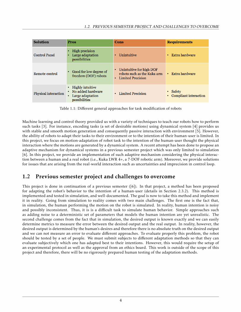
These three applications all require an understanding of user intention in order to adapt the motion; for example,a highly adaptive robot that would be used for a wide range of applications in a small industry needs to under-stand for which job it is needed for now and adapt its behavior accordingly. Different approaches exist to endowrobots with such capability. Table 1.1 summarize three general categories of solutions with their pros and cons tomodify a robotic task. Among these three solutions, two of them have added-hardware which can be a burden totransport or to learn how to use them. The goal is for the user to communicate its desired behavior in an intuitiveway without needing to learn technical details for multiple hours. For this reason, our focus will be on the thirdmethod; i.e., direct physical interaction where the robot adapts its motion according to the intentional forces ofthe human user.
(a) (b)
Figure 1: (a) Industrial Robots on a car production line [1] (b) Human working on a car with the help of a robot [2]
3
1.2. PREVIOUS SEMESTER PROJECT AND CHALLENGES TO OVERCOME
Table 1.1: Different general approaches for task modification of robots
Machine learning and control theory provided us with a variety of techniques to teach our robots how to performsuch tasks [3]. For instance, encoding tasks (a set of desirable motions) using dynamical system [4] provides uswith stable and smooth motion generation and consequently passive interaction with environment [5]. However,the ability of robots to adapt their tasks to their environment or to the intention of their human-user is limited. Inthis project, we focus on motion-adaptation of robot task to the intention of the human-user thought the physicalinteraction where the motions are generated by a dynamical system. A recent attempt has been done to propose anadaptive mechanism for dynamical systems in a previous semester project which was only limited to simulation[6]. In this project, we provide an implementation of such adaptive mechanism considering the physical interac-tion between a human and a real robot (i.e., Kuka LWR 4+, a 7-DOF robotic arm). Moreover, we provide solutionsfor issues that are arising from the real-world interaction such as uncertainties and imprecision in control loop.
1.2 Previous semester project and challenges to overcome
This project is done in continuation of a previous semester ([6]). In that project, a method has been proposedfor adapting the robot’s behavior to the intention of a human-user (details in Section 2.3.2). This method isimplemented and tested in simulation, and well-documented. The goal is now to take this method and implementit in reality. Going from simulation to reality comes with two main challenges. The first one is the fact that,in simulation, the human performing the motion on the robot is simulated. In reality, human intention is noisyand possibly inconsistent. Thus, it is is a difficult task to simulate human behavior. Simple approaches suchas adding noise to a deterministic set of parameters that models the human intention are yet unrealistic. Thesecond challenge comes from the fact that in simulation, the desired output is known exactly and we can easilydetermine metrics to measure the error between the desired output and the real output. In reality, however, thedesired output is determined by the human’s desires and therefore there is no absolute truth on the desired outputand we can not measure an error to evaluate different approaches. To evaluate properly this problem, the robotshould be tested by a set of people. We must submit subjects to different adaptation methods so that they canevaluate subjectively which one has adapted best to their intentions. However, this would require the setup ofan experimental protocol as well as the approval from an ethics board. This work is outside of the scope of thisproject and therefore, there will be no rigorously prepared human testing of the adaptation methods.
4
Chapter 2
Robot control
2.1 General robot control
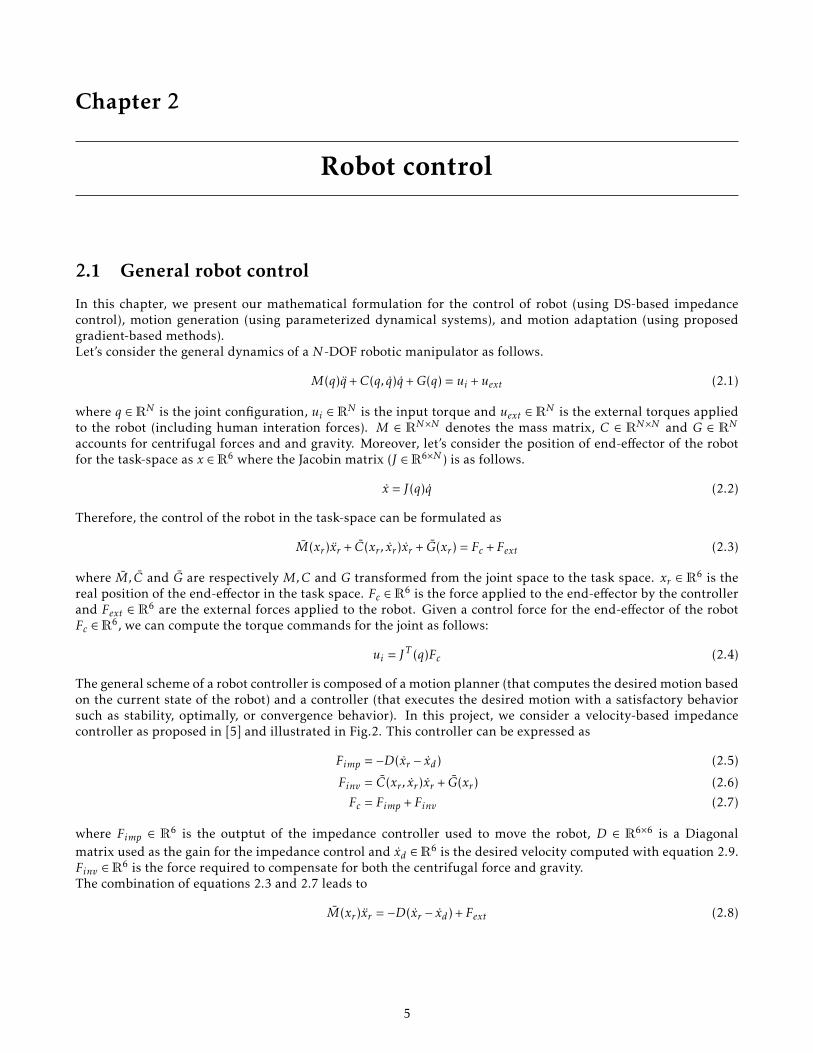
In this chapter, we present our mathematical formulation for the control of robot (using DS-based impedancecontrol), motion generation (using parameterized dynamical systems), and motion adaptation (using proposedgradient-based methods).Let’s consider the general dynamics of a N -DOF robotic manipulator as follows.
M(q)q+C(q, q)q+G(q) = ui +uext (2.1)
where q ∈ RN is the joint configuration, ui ∈ RN is the input torque and uext ∈ RN is the external torques appliedto the robot (including human interation forces). M ∈ RN×N denotes the mass matrix, C ∈ RN×N and G ∈ RNaccounts for centrifugal forces and and gravity. Moreover, let’s consider the position of end-effector of the robotfor the task-space as x ∈R6 where the Jacobin matrix (J ∈R6×N ) is as follows.
x = J(q)q (2.2)
Therefore, the control of the robot in the task-space can be formulated as
where M, C and G are respectively M,C and G transformed from the joint space to the task space. xr ∈ R6 is thereal position of the end-effector in the task space. Fc ∈R6 is the force applied to the end-effector by the controllerand Fext ∈ R6 are the external forces applied to the robot. Given a control force for the end-effector of the robotFc ∈R6, we can compute the torque commands for the joint as follows:
ui = JT (q)Fc (2.4)
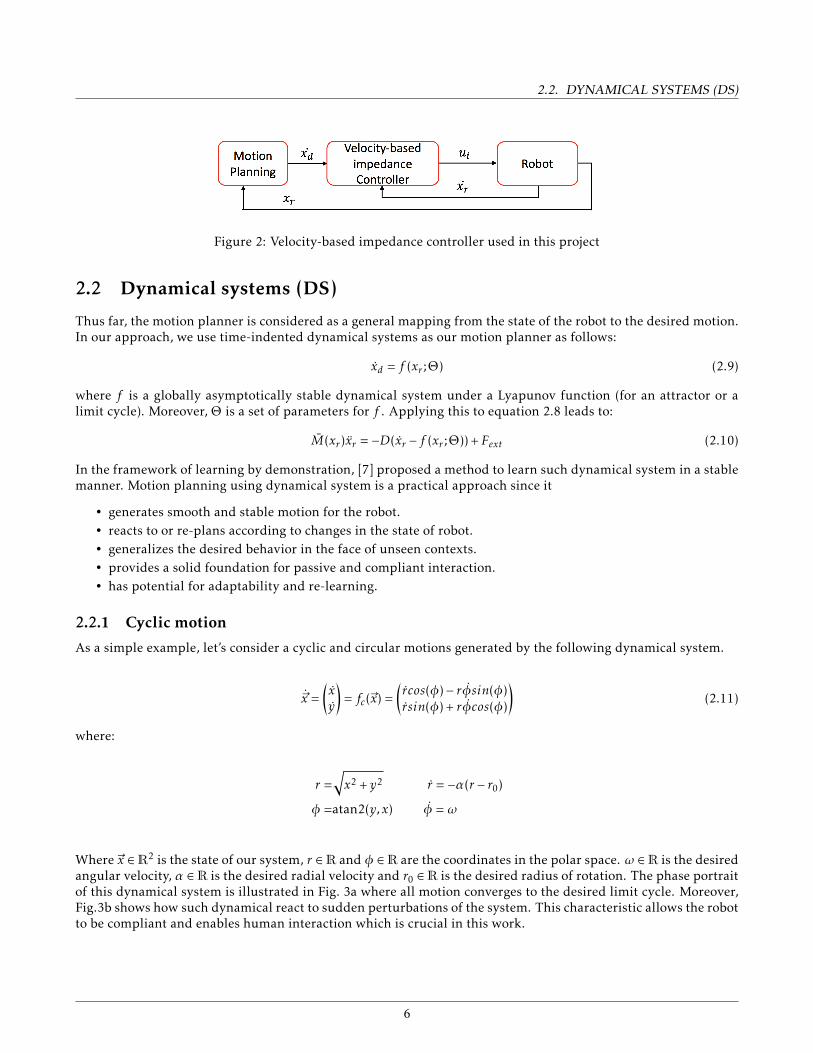
The general scheme of a robot controller is composed of a motion planner (that computes the desired motion basedon the current state of the robot) and a controller (that executes the desired motion with a satisfactory behaviorsuch as stability, optimally, or convergence behavior). In this project, we consider a velocity-based impedancecontroller as proposed in [5] and illustrated in Fig.2. This controller can be expressed as
Fimp = −D(xr − xd) (2.5)
Finv = C(xr , xr )xr + G(xr ) (2.6)
Fc = Fimp +Finv (2.7)
where Fimp ∈ R6 is the outptut of the impedance controller used to move the robot, D ∈ R6×6 is a Diagonalmatrix used as the gain for the impedance control and xd ∈R6 is the desired velocity computed with equation 2.9.Finv ∈R6 is the force required to compensate for both the centrifugal force and gravity.The combination of equations 2.3 and 2.7 leads to
M(xr )xr = −D(xr − xd) +Fext (2.8)
5
2.2. DYNAMICAL SYSTEMS (DS)
Figure 2: Velocity-based impedance controller used in this project
2.2 Dynamical systems (DS)
Thus far, the motion planner is considered as a general mapping from the state of the robot to the desired motion.In our approach, we use time-indented dynamical systems as our motion planner as follows:
xd = f (xr ;Θ) (2.9)
where f is a globally asymptotically stable dynamical system under a Lyapunov function (for an attractor or alimit cycle). Moreover, Θ is a set of parameters for f . Applying this to equation 2.8 leads to:
M(xr )xr = −D(xr − f (xr ;Θ)) +Fext (2.10)
In the framework of learning by demonstration, [7] proposed a method to learn such dynamical system in a stablemanner. Motion planning using dynamical system is a practical approach since it
• generates smooth and stable motion for the robot.• reacts to or re-plans according to changes in the state of robot.• generalizes the desired behavior in the face of unseen contexts.• provides a solid foundation for passive and compliant interaction.• has potential for adaptability and re-learning.
2.2.1 Cyclic motion
As a simple example, let’s consider a cyclic and circular motions generated by the following dynamical system.
~x =(xy
)= fc(~x) =
(rcos(φ)− rφsin(φ)rsin(φ) + rφcos(φ)
)(2.11)
where:
r =√x2 + y2 r = −α(r − r0)
φ =atan2(y,x) φ =ω
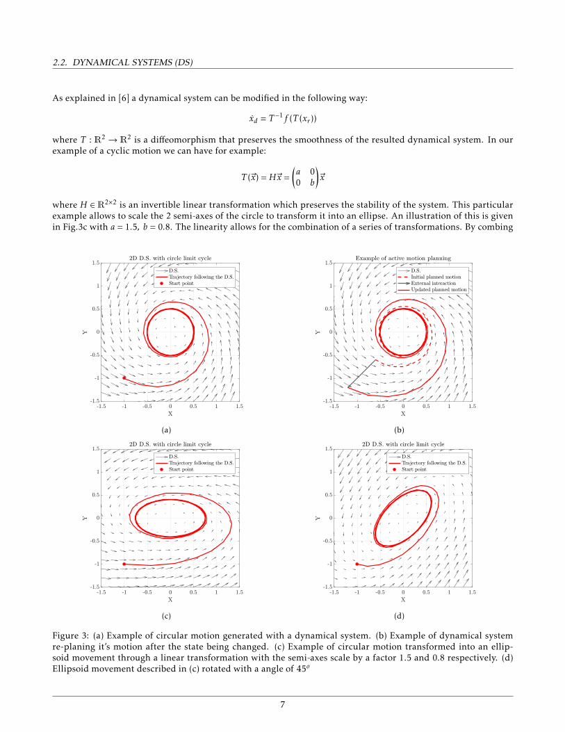
Where ~x ∈R2 is the state of our system, r ∈R and φ ∈R are the coordinates in the polar space. ω ∈R is the desiredangular velocity, α ∈R is the desired radial velocity and r0 ∈R is the desired radius of rotation. The phase portraitof this dynamical system is illustrated in Fig. 3a where all motion converges to the desired limit cycle. Moreover,Fig.3b shows how such dynamical react to sudden perturbations of the system. This characteristic allows the robotto be compliant and enables human interaction which is crucial in this work.
6
2.2. DYNAMICAL SYSTEMS (DS)
As explained in [6] a dynamical system can be modified in the following way:
xd = T −1f (T (xr ))
where T : R2 → R2 is a diffeomorphism that preserves the smoothness of the resulted dynamical system. In ourexample of a cyclic motion we can have for example:
T (~x) =H~x =(a 00 b
)~x
where H ∈R2×2 is an invertible linear transformation which preserves the stability of the system. This particularexample allows to scale the 2 semi-axes of the circle to transform it into an ellipse. An illustration of this is givenin Fig.3c with a = 1.5, b = 0.8. The linearity allows for the combination of a series of transformations. By combing
(a) (b)
(c) (d)
Figure 3: (a) Example of circular motion generated with a dynamical system. (b) Example of dynamical systemre-planing it’s motion after the state being changed. (c) Example of circular motion transformed into an ellip-soid movement through a linear transformation with the semi-axes scale by a factor 1.5 and 0.8 respectively. (d)Ellipsoid movement described in (c) rotated with a angle of 45o
7
2.2. DYNAMICAL SYSTEMS (DS)
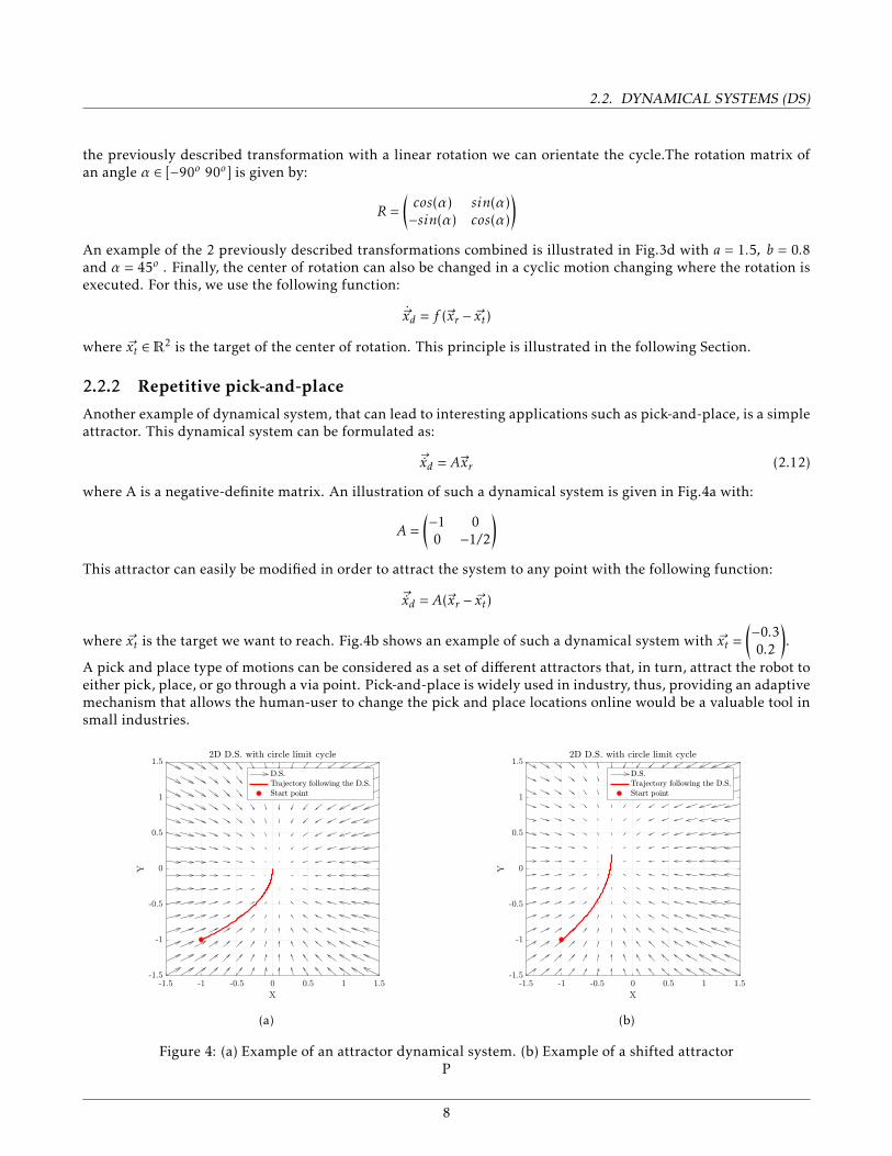
the previously described transformation with a linear rotation we can orientate the cycle.The rotation matrix ofan angle α ∈ [−90o 90o] is given by:
R =(cos(α) sin(α)−sin(α) cos(α)
)An example of the 2 previously described transformations combined is illustrated in Fig.3d with a = 1.5, b = 0.8and α = 45o . Finally, the center of rotation can also be changed in a cyclic motion changing where the rotation isexecuted. For this, we use the following function:
~xd = f (~xr − ~xt)
where ~xt ∈R2 is the target of the center of rotation. This principle is illustrated in the following Section.
2.2.2 Repetitive pick-and-place
Another example of dynamical system, that can lead to interesting applications such as pick-and-place, is a simpleattractor. This dynamical system can be formulated as:
~xd = A~xr (2.12)
where A is a negative-definite matrix. An illustration of such a dynamical system is given in Fig.4a with:
A =(−1 00 −1/2
)This attractor can easily be modified in order to attract the system to any point with the following function:
~xd = A(~xr − ~xt)
where ~xt is the target we want to reach. Fig.4b shows an example of such a dynamical system with ~xt =(−0.30.2
).
A pick and place type of motions can be considered as a set of different attractors that, in turn, attract the robot toeither pick, place, or go through a via point. Pick-and-place is widely used in industry, thus, providing an adaptivemechanism that allows the human-user to change the pick and place locations online would be a valuable tool insmall industries.
(a) (b)
Figure 4: (a) Example of an attractor dynamical system. (b) Example of a shifted attractorP
8
2.3. MOTION ADAPTION USING DYNAMICAL SYSTEMS
(a) (b)
Figure 5: (a) Example of a local adaptation(orange area) of a dynamical system[8]. (b) Different dynamical systemsused to perform task adaptation in [9]
2.3 Motion adaption using dynamical systems
2.3.1 State of the art
Although numerous works have been done to perform motion-adaptation, here we only focus on those usingdynamical systems. In [8], authors investigated local adaptation of dynamical systems for grasping objects de-pending on the shape of the object while avoiding obstacles of unknown size and shapes. The illustration of thelocal adaptation of a dynamical system is shown in Fig.5a. For instance, a local modulation can be applied to theDS to avoid an obstacle that would be along the initial trajectories.
A second example of adaptation of dynamical systems is illustrated in [9]. In this work, the adaptation is notdirectly performed on a single DS, but on a linear combination of several ones. The goal is to switch betweendifferent dynamical systems based on human interaction. A general motion planner measures the likelihood ofdifferent DS. When the human wants to switch motion, it can safely grab the robot and move it according to thedesired motion. The planer measures the likelihood increase of the desired motion and smoothly switches fromone stable DS to the other. The different DS used in the mentioned work are illustrated in Fig.5b.
In contrast to previous works, the adaptation in this work is done 1) globally (not just locally) which allowsfor higher level of generalization and 2) without switching which enables the robot to reshape one specific taskaccording to the intention of the human.
2.3.2 Solution studied in previous semester project
As mentioned in Section 1.2, this work is done in the continuity of a previous semester project that simulated theadaptation of dynamical systems. In this approach, the goal is to adapt the set of parameters Θ upon which the DSdepends. For example, in the circular motion described in Section 2.2, the parameter that describes the shape ofthe trajectory is the r0 coefficient. By changing this parameter, one can modify the shape of the dynamical systemand adapts it to the user’s intentions.
In order to achieve this, optimization algorithms were used to minimize the error between the real velocity (whichaccounts for the human intention since it can be influenced by human interaction in our compliant architecture)and the desired velocity (which is generated by dynamical system given its parameters). This is described by thefollowing cost function:
J(xr , xr ;Θ) =12eT e =
12|xr − xd |2 (2.13)
9
2.3. MOTION ADAPTION USING DYNAMICAL SYSTEMS
where e = xr − xd is the error between the real and the desired velocities, |.| denotes the norm of a vector. In theprevious work, the gradient of this function was used in order to update the parameters. The gradient of thisfunction is defined as:
∇ΘJ =∂J∂Θ
(2.14)
=(∂J∂θ1
∂J∂θ2
· · · ∂J∂θn
)T(2.15)
where n is the number of parameters and θi is the ith parameter of the dynamical system. To compute the gradientwith respect to each parameter, we can write:
∂J∂θi
= eT · ∂e∂θi
(2.16)
= eT ·∂f (xr ;Θ)∂θi
(2.17)
The analytical formulation of ∂f (xr ,Θ)∂θi
for nontrivial DS is usually not available. Therefore, we use the centereddifferences approximation:
∂J∂θi
=eT ·f (xr ;Θ,i ,θi + h)− f (xr ;Θ,i ,θi − h)
2h(2.18)
where h is the step size of the gradient, and Θ,i denotes all other parameters (except θi) that are kept at theirprevious value.
The results of this project show that the best adaptation algorithms depends on the motion that is being adapted.In a fast evolving motion, such as point to point faster algorithms perform better. However, in the case of cyclicmotions, the adaptation must be slow to avoid instability issues. The first motion that will be adapted to in realitywill be the cyclic motion and therefore the adaptation method that will be implemented is the gradient descentmethod. In this method, the parameters are updated proportionally to the gradient of the cost function. This givesus:
Θ = −ε∇ΘJ (2.19)
where ε is the rate of adaptation of the gradient descent which leads us to the following discrete formulation:
θnew = θold − εeT ·∂f (xr ;Θ)∂θi
(2.20)
Therefore there are 2 hyperparameters for this method, the gradient step h and the rate of adaptation ε.
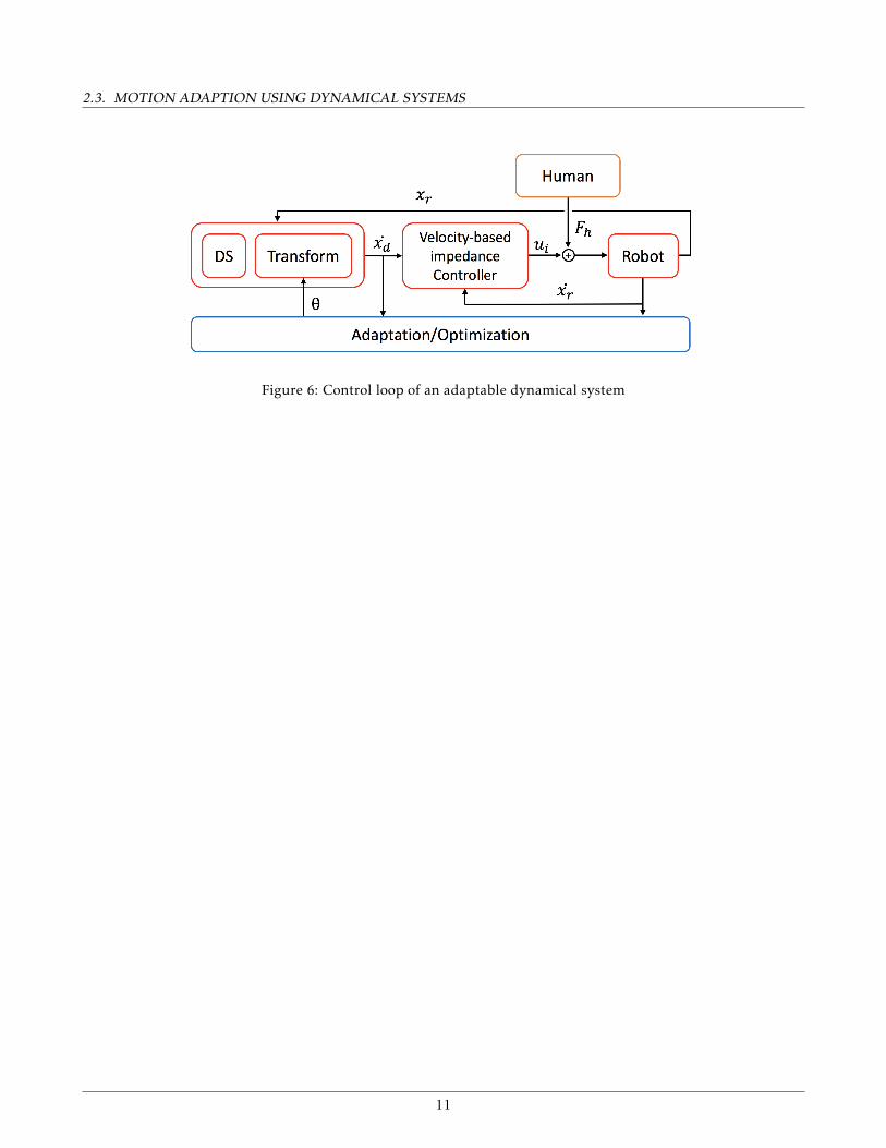
The control loop shown in Fig.2 can be modified to include this adaptation step as illustrated by Fig.6. An adapta-tion/optimization block is added to the system that takes as input the real velocity of the robot xr and the desiredvelocity of the robot xd . The human is also added to the control loop where it applies an unknown force Fh to therobot in order to demonstrate his/her desired motions.
10
2.3. MOTION ADAPTION USING DYNAMICAL SYSTEMS
Figure 6: Control loop of an adaptable dynamical system
11
Chapter 3
Implementation of the adaptation
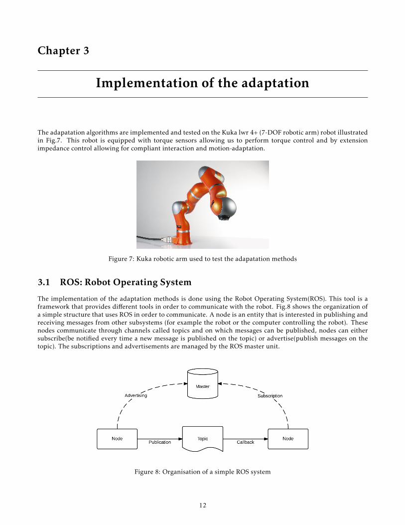
The adapatation algorithms are implemented and tested on the Kuka lwr 4+ (7-DOF robotic arm) robot illustratedin Fig.7. This robot is equipped with torque sensors allowing us to perform torque control and by extensionimpedance control allowing for compliant interaction and motion-adaptation.
Figure 7: Kuka robotic arm used to test the adapatation methods
3.1 ROS: Robot Operating System
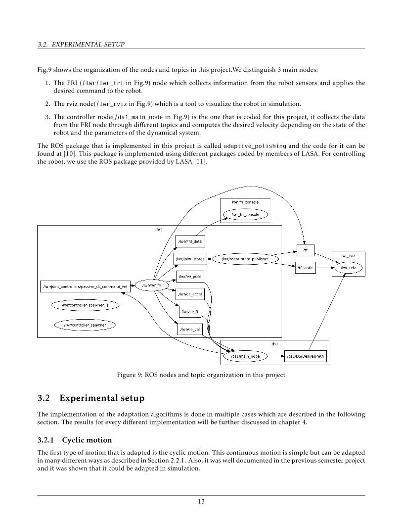
The implementation of the adaptation methods is done using the Robot Operating System(ROS). This tool is aframework that provides different tools in order to communicate with the robot. Fig.8 shows the organization ofa simple structure that uses ROS in order to communicate. A node is an entity that is interested in publishing andreceiving messages from other subsystems (for example the robot or the computer controlling the robot). Thesenodes communicate through channels called topics and on which messages can be published, nodes can eithersubscribe(be notified every time a new message is published on the topic) or advertise(publish messages on thetopic). The subscriptions and advertisements are managed by the ROS master unit.
Figure 8: Organisation of a simple ROS system
12
3.2. EXPERIMENTAL SETUP
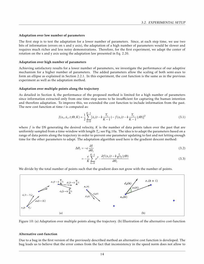
Fig.9 shows the organization of the nodes and topics in this project.We distinguish 3 main nodes:
1. The FRI (/lwr/lwr_fri in Fig.9) node which collects information from the robot sensors and applies thedesired command to the robot.
2. The rviz node(/lwr_rviz in Fig.9) which is a tool to visualize the robot in simulation.
3. The controller node(/ds1_main_node in Fig.9) is the one that is coded for this project, it collects the datafrom the FRI node through different topics and computes the desired velocity depending on the state of therobot and the parameters of the dynamical system.
The ROS package that is implemented in this project is called adaptive_polishing and the code for it can befound at [10]. This package is implemented using different packages coded by members of LASA. For controllingthe robot, we use the ROS package provided by LASA [11].
Figure 9: ROS nodes and topic organization in this project
3.2 Experimental setup
The implementation of the adaptation algorithms is done in multiple cases which are described in the followingsection. The results for every different implementation will be further discussed in chapter 4.
3.2.1 Cyclic motion
The first type of motion that is adapted is the cyclic motion. This continuous motion is simple but can be adaptedin many different ways as described in Section 2.2.1. Also, it was well documented in the previous semester projectand it was shown that it could be adapted in simulation.
13
3.2. EXPERIMENTAL SETUP
Adaptation over low number of parameters
The first step is to test the adaptation for a lower number of parameters. Since, at each step time, we use twobits of information (errors on x and y axis), the adaptation of a high number of parameters would be slower andrequires much richer and less noisy demonstrations. Therefore, for the first experiment, we adapt the center ofrotation on the x and y axis using the adaptation law presented in Eq. 2.20.
Adaptation over high number of parameters
Achieving satisfactory results for a lower number of parameters, we investigate the performance of our adaptivemechanism for a higher number of parameters. The added parameters allow the scaling of both semi-axes toform an ellipse as explained in Section 2.2.1. In this experiment, the cost function is the same as in the previousexperiment as well as the adaptation method.
Adaptation over multiple points along the trajectory
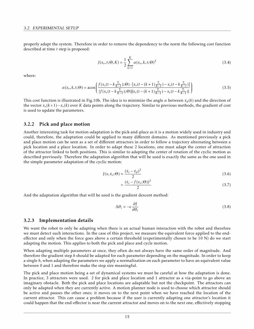
As detailed in Section 4, the performance of the proposed method is limited for a high number of parameterssince information extracted only from one time-step seems to be insufficient for capturing the human intentionand therefore adaptation. To improve this, we extended the cost function to include information from the past.The new cost function at time t is computed as:
J(xr , xr , t;Θ,K) =12
K−1∑k=0
[xr (t − kTsK − 1
)− f (xr (t − kTsK − 1
);Θ)]2 (3.1)
where f is the DS generating the desired velocity, K is the number of data points taken over the past that areuniformly sampled from a time-window with length Ts; see Fig.10a. The idea is to adapt the parameters based on arange of data points along the trajectory in order to prevent one parameter updating to fast and not letting enoughtime for the other parameters to adapt. The adaptation algorithm used here is the gradient descent method:
∆θi = −ε ∂J∂θi
(3.2)
= − εK
K−1∑k=0
eT ·∂f (xr (t − k
TsK−1 );Θ)
∂θi(3.3)
We divide by the total number of points such that the gradient does not grow with the number of points.
(a) (b)
Figure 10: (a) Adaptation over multiple points along the trajectory. (b) Illustration of the alternative cost-function
Alternative cost-function
Due to a bug in the first version of the previously described method an alternative cost function is developed. Thebug leads us to believe that the error comes from the fact that inconsistency in the speed norm does not allow to
14
3.2. EXPERIMENTAL SETUP
properly adapt the system. Therefore in order to remove the dependency to the norm the following cost functiondescribed at time t step is proposed:
J(xr , t;Θ,K) =12
K∑k=1
α(xr , k, t;Θ)2 (3.4)
where:
α(xr , k, t;Θ) = acos
f (xr (t − kTsK−1 );Θ) · [xr (t − (k + 1) Ts
K−1 )− xr (t − kTsK−1 )]
|f (xr (t − kTsK−1 );Θ)||xr (t − (k + 1) Ts
K−1 )− xr (t − kTsK−1 )|
(3.5)
This cost function is illustrated in Fig.10b. The idea is to minimize the angle α between xd(k) and the direction ofthe vector xr (k+1)−xr (k) over K data points along the trajectory. Similar to previous methods, the gradient of costis used to update the parameters.
3.2.2 Pick and place motion
Another interesting task for motion-adaptation is the pick-and-place as it is a motion widely used in industry andcould, therefore, the adaptation could be applied to many different domains. As mentioned previously a pickand place motion can be seen as a set of different attractors in order to follow a trajectory alternating between apick location and a place location. In order to adapt these 2 locations, one must adapt the center of attractionof the attractor linked to both positions. This is similar to adapting the center of rotation of the cyclic motion asdescribed previously. Therefore the adaptation algorithm that will be used is exactly the same as the one used inthe simple parameter adaptation of the cyclic motion:
J(x, xr ;Θ) =(xr − xd)2
2(3.6)
=(xr − f (xr ;Θ))2
2(3.7)
And the adaptation algorithm that will be used is the gradient descent method:
∆θi = −ε ∂J∂θi
(3.8)
3.2.3 Implementation details
We want the robot to only be adapting when there is an actual human interaction with the robot and thereforewe must detect such interactions. In the case of this project, we measure the equivalent force applied to the end-effector and only when the force goes above a certain threshold (experimentally chosen to be 10 N) do we startadapting the motion. This applies to both the pick and place and cycle motion.
When adapting multiple parameters at once, they often do not always have the same order of magnitude. Andtherefore the gradient step h should be adapted for each parameter depending on the magnitude. In order to keepa single h, when adapting the parameters we apply a normalization on each parameter to have an equivalent valuebetween 0 and 1 and therefore make the step size meaningful.
The pick and place motion being a set of dynamical systems we must be careful at how the adaptation is done.In practice, 3 attractors were used. 2 for pick and place location and 1 attractor as a via-point to go above animaginary obstacle. Both the pick and place locations are adaptable but not the checkpoint. The attractors canonly be adapted when they are currently active. A motion planner node is used to choose which attractor shouldbe active and pauses the other ones; it moves on to the next point when we have reached the location of thecurrent attractor. This can cause a problem because if the user is currently adapting one attractor’s location itcould happen that the end-effector is near the current attractor and moves on to the next one, effectively stopping
15
3.2. EXPERIMENTAL SETUP
the adaptation half-way through. To prevent this, the force applied to the end-effector must be below a certainthreshold. This signal that the human has let go of the robot and is therefore satisfied with the new location foreither place or pick. In short, the post-condition for sub-task is to reach the attractor and to have small interactionforces.
16
Chapter 4
Results
4.1 Cyclic motion
4.1.1 Adaptation over low number of parameters
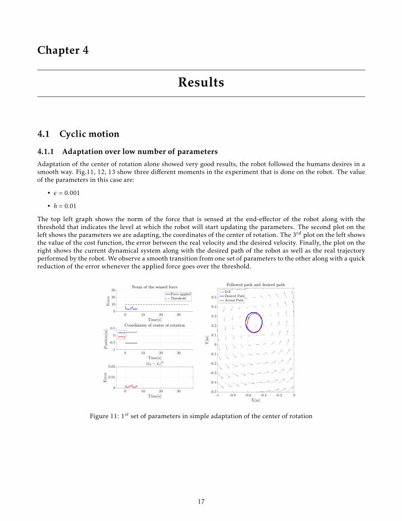
Adaptation of the center of rotation alone showed very good results, the robot followed the humans desires in asmooth way. Fig.11, 12, 13 show three different moments in the experiment that is done on the robot. The valueof the parameters in this case are:
• ε = 0.001
• h = 0.01
The top left graph shows the norm of the force that is sensed at the end-effector of the robot along with thethreshold that indicates the level at which the robot will start updating the parameters. The second plot on theleft shows the parameters we are adapting, the coordinates of the center of rotation. The 3rd plot on the left showsthe value of the cost function, the error between the real velocity and the desired velocity. Finally, the plot on theright shows the current dynamical system along with the desired path of the robot as well as the real trajectoryperformed by the robot. We observe a smooth transition from one set of parameters to the other along with a quickreduction of the error whenever the applied force goes over the threshold.
Figure 11: 1st set of parameters in simple adaptation of the center of rotation
17
4.1. CYCLIC MOTION
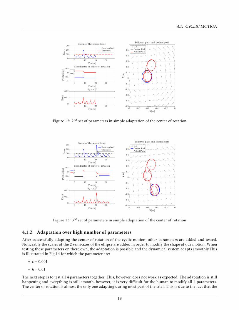
Figure 12: 2nd set of parameters in simple adaptation of the center of rotation
Figure 13: 3rd set of parameters in simple adaptation of the center of rotation
4.1.2 Adaptation over high number of parameters
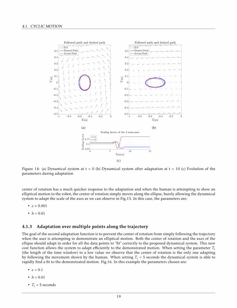
After successfully adapting the center of rotation of the cyclic motion, other parameters are added and tested.Noticeably the scales of the 2 semi-axes of the ellipse are added in order to modify the shape of our motion. Whentesting these parameters on there own, the adaptation is possible and the dynamical system adapts smoothly.Thisis illustrated in Fig.14 for which the parameter are:
• ε = 0.001
• h = 0.01
The next step is to test all 4 parameters together. This, however, does not work as expected. The adaptation is stillhappening and everything is still smooth, however, it is very difficult for the human to modify all 4 parameters.The center of rotation is almost the only one adapting during most part of the trial. This is due to the fact that the
18
4.1. CYCLIC MOTION
(a) (b)
(c)
Figure 14: (a) Dynamical system at t = 0 (b) Dynamical system after adaptation at t = 10 (c) Evolution of theparameters during adaptation
center of rotation has a much quicker response to the adaptation and when the human is attempting to show anelliptical motion to the robot, the center of rotation simply moves along the ellipse, barely allowing the dynamicalsystem to adapt the scale of the axes as we can observe in Fig.15. In this case, the parameters are:
• ε = 0.001
• h = 0.01
4.1.3 Adaptation over multiple points along the trajectory
The goal of the second adaptation function is to prevent the center of rotation from simply following the trajectorywhen the user is attempting to demonstrate an elliptical motion. Both the center of rotation and the axes of theellipse should adapt in order for all the data points to "fit" correctly to the proposed dynamical system. This newcost function allows the system to adapt efficiently to the demonstrated motion. When setting the parameter Ts(the length of the time window) to a low value we observe that the center of rotation is the only one adaptingby following the movement shown by the human. When setting Ts = 5 seconds the dynamical system is able torapidly find a fit to the demonstrated motion. Fig.16. In this example the parameters chosen are:
• ε = 0.1
• h = 0.01
• Ts = 5 seconds
19
4.1. CYCLIC MOTION
(a) (b) (c)
(d) (e) (f)
Figure 15: Evolution of the dynamical system with the first cost cost function while adapting multiple parameters,we can see the center of rotation moving along the trajectory
• K = 10 points
In Fig.17 we show the adaptation of the cyclic motion with the angle of the rotation as added parameter bring thetotal number of parameters to adapt up to 5. The set of parameters used are the same as for the previous example.
4.1.4 Alternative cost-function
Due to lack of time the alternative cost function is not tuned sufficiently. The initial results show that the adapta-tion isn’t very consistent and doesn’t always manage to converge to the ideal solution. Fig.18 shows an example inwhich the adaptation is successful, but later on when a new motion was shown isn’t able to converge to the desiredsolution. In this case, the parameters used are:
• ε = 0.001
• h = 0.01
• Ts = 5 seconds
• K = 20 points
20
4.2. PICK AND PLACE MOTION
(a) (b) (c)
(d)
Figure 16: (a) & (b) & (c) Dynamical system at respectively t = 15s, t = 30s and t = 47s (d) Evolution of theparameters during adaptation
4.2 Pick and place motion
Adaptation of the attractors during the repetitive pick and place motion show that it is possible to adapt eachattractor independently and therefore modify the pick and place locations with ease and very intuitively. However,it is noticed that there is sometimes not enough time to grab the robot before it reaches the attractor and thereforeare not able to update it. The set of parameters that work for this adaptation are:
• ε = 0.001
• h = 0.01
For a demonstration of the pick and place adaptation see [12].
21
4.2. PICK AND PLACE MOTION
(a) (b)
(c) (d)
Figure 17: (a) & (b) & (c) Dynamical system at respectively t = 10s, t = 25s and t = 39s (d) Evolution of theparameters during adaptation
22
4.2. PICK AND PLACE MOTION
(a) (b)
(c)
Figure 18: (a) Example of when the alternative cost function allows for good adaptation (t = 15) (b) Example ofwhen the alternative cost function doesn’t allows for good adaptation (t = 26) (c) Evolution of the parametersduring adaptation
23
Chapter 5
Conclusion and future work
Conclusion
This project shows that motion-adaptation using parametric dynamical system is not only possible but it couldbe very effective for compliant human-robot interaction. We showed by sampling few data points form humanbehavior (captured by the real velocity) and motion-generator (the desired velocity), our simple adaptation mech-anism is able to comply to the intention of the human. We observed that quality of the adaptation depends on thechoice of the cost function, type of the motion, and hyperparameters. When adapting on a low number of param-eters, a single data point can be taken in order to minimize the cost function. However, with the increase in thenumber of parameters to adapt, we need more information order to properly adapt the dynamical system to thedemonstrated motion. The cost function 3.1 derived in this project allows such an adaptation by optimizing overa set of points along the trajectory instead of only the most recent point as proposed by [6]. With this modifiedcost function, we are able to successfully adapt cyclic dynamical systems with a set of 5 different parameters:
• The center of rotation of the rotation in both x and y.
• The angle of the orientation of the rotation of the cyclic motion.
• The scale of both semi-axes of the ellipse.
We have also shown that adaptation of a simple attractor is possible and that by extension this can allow to adaptmore complex motions such as a repetitive pick and place which could be valuable for industrial applications.
Future work
Further attempts are required to reach a systematic approach for tuning the parameters to obtain a workingsolution based on the cost function 3.4. Also, a rigorous tuning of the hyper-parameters should be done in orderto find the best working solution. Intuition on how the parameters were chosen for this project and where to startto optimize them further is the following:
• ε: When this parameter goes to 0, there is no more adaptation as the change in the parameters is directlyproportional to the value of epsilon. However, if this parameter is set too high, then the parameters do notupdate smoothly and the dynamical system varies extremely quickly creating a very jerky motion that isvery unpleasant to the user.
• h: The gradient step must be sufficiently small to have a precise approximation for the derivative of the costfunction. However, since we are dealing with noisy observation, reducing this parameter would result innoisy approximation for the derivative.
• Ts and K : These two parameters go hand in hand. In order to adapt properly the dynamical system, theadaptation must be done on a set of points that both characterizes well the DS (from the desired velocity)and captures well the human intention (from the real velocity). Therefore, Ts must be sufficiently largeto capture a sufficient portion of the cycle and K must allow the sampling of enough data points. On theother hand, increasing the number of data point increases leas to issues with the computational effort andincluding contradictory demonstrations form the past that needs to be forgotten.
Finally, future work can be done to improve the compliant behavior of the robot during the adaptation. The ideawould be to lower the impedance gains (D in equation 2.5), thus, reducing the stiffness of the robot. This wouldbring 2 advantages: 1) it would reduce the human effort required to demonstrate his/her desired behavior, 2) thevariation of the compliance serve as a haptic communication where human can infer the state of robot (e.g., the
24
robot’s confidence with respect to the parameters that it is optimizing). However, the variation of the complianceshould be done in a smooth and stable manner to avoid creating jerky and sudden motion while in contact with ahuman. Also, it is required to find a method where the impedance gains are updated based on the quality of theadaptation; e.g., based the value of the cost function. For example, if the human is unable to demonstrate a consistmotion that the adaptation mechanism cannot converge to, the robot’s stiffness should be decreased even furtherin order to allow the human to demonstrate the motion in a better way.
Antoine Laurens
Date and Signature
25
Bibliography
[1] Industrial production line. url: http://imgur.com/CF8tEct.
[2] Robot assisting human in industry. url: https://www.manufacturingtomorrow.com/article/2016/02/collaborative-robots-working-in-manufacturing/7672/.
[3] Aude Billard et al. “Robot programming by demonstration”. In: Springer handbook of robotics. Springer, 2008,pp. 1371–1394.
[4] S Mohammad Khansari-Zadeh and Aude Billard. “Learning stable nonlinear dynamical systems with gaus-sian mixture models”. In: IEEE Transactions on Robotics 27.5 (2011), pp. 943–957.
[5] Klas Kronander and Aude Billard. “Passive interaction control with dynamical systems”. In: IEEE Roboticsand Automation Letters 1.1 (2016), pp. 106–113.
[6] Thomas Triquet, Mahdi Khoramshahi, and Aude Billard. Task-adaptation for assistive robotics using switchingdynamical systems. Tech. rep. LASA - EPFL, 2017, p. 28. url: https://www.dropbox.com/s/97hrwhsg2gz9c8g/Triquet_TaskAdaptationForAssitiveRoboticsUsingSwitchingDS.pdf?dl=0.
[7] Nicolas Sommer, Klas Kronander, and Aude Billard. “Learning Externally Modulated Dynamical Systems”.In: Proceedings of the IEEE/RSJ International Conference on Intelligent Robots and Systems (2017). url: https://infoscience.epfl.ch/record/229361 (visited on 12/29/2017).
[8] K. Kronander, M. Khansari, and A. Billard. “Incremental motion learning with locally modulated dynamicalsystems”. In: Robotics and Autonomous Systems 70 (Aug. 2015), pp. 52–62. issn: 0921-8890. doi: 10.1016/j.robot.2015.03.010. url: http://www.sciencedirect.com/science/article/pii/S0921889015000822.
[9] M. Khoramshahi and A. Billard. “A Dynamical System Approach to Task-Adaptation in Physical Human-Robot Interaction”. In: under review in Autonomous Robots (2018).
[10] GitHub repository of the adaptive polishing package. url: https : / / github . com / alaurens / adaptive _polishing.
[11] GitHub repository of the ROS package to control KUKA LWR. url: https://github.com/epfl-lasa/kuka-lwr-ros.
[12] Demonstration of pick and place adaptation. url: https://youtu.be/HLfZW6rPxYc.
26
The demonstrations of this work can be viewed here:https://youtu.be/qIcOAtVMNgE