Adaptive Lasso and group-Lasso for functional Poisson

regression

S. Ivanoff‡, F. Picard? & V. Rivoirard‡

‡CEREMADE UMR CNRS 7534, Universite Paris Dauphine,F-75775 Paris, France?LBBE, UMR CNRS 5558 Univ. Lyon 1, F-69622 Villeurbanne, France

December 22, 2014

Abstract

High dimensional Poisson regression has become a standard framework for the analysis ofmassive counts datasets. In this work we estimate the intensity function of the Poissonregression model by using a dictionary approach, which generalizes the classical basis ap-proach, combined with a Lasso or a group-Lasso procedure. Selection depends on penaltyweights that need to be calibrated. Standard methodologies developed in the Gaussianframework can not be directly applied to Poisson models due to heteroscedasticity. Here weprovide data-driven weights for the Lasso and the group-Lasso derived from concentrationinequalities adapted to the Poisson case. We show that the associated Lasso and group-Lassoprocedures are theoretically optimal in the oracle approach. Simulations are used to assessthe empirical performance of our procedure, and an original application to the analysis ofNext Generation Sequencing data is provided.

Introduction

Poisson functional regression has become a standard framework for image or spectra analysis,in which case observations are made of n independent couples (Yi, Xi)i=1,...,n, and can bemodeled as

Yi|Xi ∼ Poisson(f0(Xi)). (0.1)

The Xi’s (random or fixed) are supposed to lie in a known compact support of Rd (d ≥ 1), say[0, 1]d, and the purpose is to estimate the unknown intensity function f0 assumed to be pos-itive. Wavelets have been used extensively for intensity estimation, and the statistical chal-lenge has been to propose thresholding procedures in the spirit of [Donoho and Johnstone, 1994],that were adapted to the variance’s spatial variability associated with the Poisson frame-work. An early method to deal with high dimensional count data has been to apply avariance stabilizing-transform (see [Anscombe, 1948]) and to treat the transformed data asif they were Gaussian. More recently, the same idea has been applied to the data’s decom-position in the Haar-wavelet basis, see [Fryzlewicz and Nason, 2004] and [Fryzlewicz, 2008],but these methods rely on asymptotic approximations and tend to show lower performancewhen the level of counts is low [Besbeas et al., 2004]. Dedicated wavelet thresholding meth-ods were developed in the Poisson setting by [Kolaczyk, 1999] and [Sardy et al., 2004], and

1

a recurrent challenge has been to define an appropriate threshold like the universal thresholdfor shrinkage and selection, as the heteroscedasticity of the model calls for component-wisethresholding.

In this work we first propose to enrich the standard wavelet approach by consideringthe so-called dictionary strategy. We assume that log f0 can be well approximated by alinear combination of p known functions, and we reduce the estimation of f0 to the estima-tion of p coefficients. Dictionaries can be built from classical orthonormal systems such aswavelets, histograms or the Fourier basis, which results in a framework that encompasseswavelet methods. Considering overcomplete (ie redundant) dictionaries is efficient to cap-ture different features in the signal, by using sparse representations (see [Chen et al., 2001]or [Tropp, 2004]). For example, if log f0 shows piece-wise constant trends along with someperiodicity, combining both Haar and Fourier bases will be more powerful than separatestrategies, and the model will be sparse in the coefficients domain. To ensure sparse es-timations, we consider the Lasso and the group-Lasso procedures. Group estimators areparticularly well adapted to the dictionary framework, especially if we consider dictionar-ies based on a wavelet system, for which it is well known that coefficients can be groupedscale-wise for instance (see [Chicken and Cai, 2005]). Finally, even if we do not make anyassumption on p itself, it may be larger than n and methodologies based on `1-penalties,such as the Lasso and the group-Lasso appear appropriate.

The statistical properties of the Lasso are particularly well understood in the context ofregression with i.i.d. errors, or for density estimation for which a range of oracle inequal-ities have been established. These inequalities, now widespread in the literature, providetheoretical error bounds that hold on events with a controllable (large) probability. See forinstance [Bertin et al., 2011], [Bickel et al., 2009], [Bunea et al., 2007a, Bunea et al., 2007b]and the references therein. For generalized linear models, [Park and Hastie, 2007] studied`1-regularization path algorithms and [van de Geer, 2008] established non-asymptotic oracleinequalities. The sign consistency of the Lasso has been studied by [Jia et al., 2013] for a veryspecific Poisson model. Finally, we also mention than the Lasso has also been extensivelyconsidered in survival analysis. See for instance [Gaıffas and Guilloux, 2012], [Zou, 2008],[Kong and Nan, 2014], [Bradic et al., 2011], [Lemler, 2013] and [Hansen et al., 2014].

Here we consider not only the Lasso estimator but also its extension, the group-Lassoproposed by [Yuan and Lin, 2006], which is relevant when the set of parameters can bepartitioned into groups. The analysis of the group-Lasso has been led in different con-texts. For instance, consistency has been studied by [Bach, 2008], [Obozinski et al., 2011]and [Wei and Huang, 2010]. In the linear model, [Nardi and Rinaldo, 2008] derived condi-tions ensuring various asymptotic properties such as consistency, oracle properties or per-sistence. Still for the linear model, [Lounici et al., 2011] established oracle inequalities and,in the Gaussian setting, pointed out advantages of the group-Lasso with respect to theLasso, generalizing the results of [Chesneau and Hebiri, 2008] and [Huang and Zhang, 2010].We also mention [Meier et al., 2008] who studied the group-Lasso for logistic regression,[Blazere et al., 2014] for generalized linear model with Poisson regression as a special caseand [Dalalyan et al., 2013] for other linear heteroscedastic models.

As pointed out by empirical comparative studies [Besbeas et al., 2004], the calibrationof any thresholding rule is of central importance. Here we consider Lasso and group-Lassopenalties of the form

pen(β) =

p∑j=1

λj |βj |

2

and

peng(β) =

K∑k=1

λgk‖βGk‖2,

where G1 ∪ · · · ∪ GK is a partition of 1, . . . , p into non-overlapping groups (see Sec-tion 1 for more details). By calibration we refer to the definition and to the suitablechoice of the weights λj and λgk, which is intricate in heteroscedastic models, especiallyfor the group-Lasso. For functional Poissonian regression, the ideal shape of these weightsis unknown, even if for the group-Lasso, the λgk’s should of course depend on the groupssize. As for the Lasso, most proposed weights in the literature are non-random and con-stant such that the penalty is proportional to ‖β‖1, but when facing variable selectionand consistency simultaneously, [Zou, 2006] showed the interest in considering non-constantdata-driven `1-weights even in the simple case where the noise is Gaussian with constantvariance. This issue becomes even more critical in Poisson functional regression in whichvariance shows spatial heterogeneity. As [Zou, 2006], our first contribution is to proposehere adaptive procedures with weights depending on the data. Weights λj for the Lasso arederived by using sharp concentration inequalities, in the same spirit as [Bertin et al., 2011],[Gaıffas and Guilloux, 2012], [Lemler, 2013] and [Hansen et al., 2014], but adapted to thePoissonian setting. To account for heteroscedasticity, weights λj are component-specificand depend on the data (see Theorem 1). We propose a similar procedure for the calibra-tion of the group-Lasso. In most proposed procedures, the analogs of the λgk’s are propor-

tional to the√|Gk|’s (see [Nardi and Rinaldo, 2008], [Buhlmann and van de Geer, 2011] or

[Blazere et al., 2014]). But to the best of our knowledge, adaptive group-Lasso procedures(with weights depending on the data) have not been proposed yet. This is the purpose ofTheorem 2, which is the main result of this work, generalizing Theorem 1 by using sharpconcentration inequalities for infinitely divisible vectors. We show the shape relevance of thedata-driven weights λgk by comparing them to the weights proposed by [Lounici et al., 2011]in the Gaussian framework. In Theorem 2, we do not impose any condition on the groupssize. However, whether |Gk| is smaller than log p or not highly influences the order ofmagnitude of λgk.

Our second contribution consists in providing the theoretical validity of our approach byestablishing slow and fast oracle inequalities under RE-type conditions in the same spiritas [Bickel et al., 2009]. Closeness between our estimates and f0 is measured by using theempirical Kullback-Leibler divergence. We show that classical oracle bounds are achieved.We also show the relevance of considering the group-Lasso instead of the Lasso in somesituations. Our results, that are non-asymptotic, are valid under very general conditionson the design (Xi)i=1,...,n and on the dictionary. However, to shed some light on our re-sults, we illustrate some of them in the asymptotic setting with classical dictionaries likewavelets, histograms or Fourier bases. Our approach generalizes the classical basis approachand in particular block wavelet thresholding which is equivalent to group-Lasso in that case(see [Yuan and Lin, 2006]). We refer the reader to [Chicken and Cai, 2005] for a deep studyof block wavelet thresholding in the context of density estimation whose framework showssome similarities with ours in terms of heteroscedasticity. Note that sharp estimation ofvariance terms proposed in this work can be viewed as an extension of coarse bounds pro-vided by [Chicken and Cai, 2005]. Finally, we emphasize that our procedure differs from[Blazere et al., 2014]’s one in several aspects: First, in their Poisson regression setting, theydo not consider a dictionary approach. Furthermore, their weights are constant and notdata-driven, so are strongly different from ours. Finally, rates of [Blazere et al., 2014] areestablished under much more stronger assumptions than ours (see Section 3.1 for moredetails).

3

Finally, we explore the empirical properties of our calibration procedures by using sim-ulations. We show that our procedures are very easy to implement, and we compare theirperformance with variance-stabilizing transforms and cross-validation. The calibrated Lassoand group-Lasso are associated with excellent reconstruction properties, even in the caseof low counts. We also propose an original application of functional Poisson regressionto the analysis of Next Generation Sequencing data, with the search of peaks in Pois-son counts associated with the detection of replication origins in the human genome (see[Picard et al., 2014]).

This article is organized as follows. In Section 1, we introduce the Lasso and group-Lassoprocedures we propose in the dictionary approach setting. In Section 2, we derive data-drivenweights of our procedures that are extensively commented. Theoretical performance of ourestimates are studied in Section 3 in the oracle approach. In Section 4, we investigate theempirical performance of the proposed estimators using simulated data, and an applicationis provided on next generation sequencing data in Section 5.

1 Penalized log-likelihood estimates for Poisson regres-sion and dictionary approach

We consider the functional Poisson regression model, with n observed counts Yi ∈ N modeledsuch that:

Yi|Xi ∼ Poisson(f0(Xi)), (1.1)

with the Xi’s (random or fixed) supposed to lie in a known compact support, say [0, 1]d.Since the goal here is to estimate the function f0 assumed to be positive on [0, 1]d, a naturalcandidate is a function f of the form f = exp(g). Then, we consider the so-called dictionaryapproach which consists in decomposing g as a linear combination of the elements of agiven finite dictionary of functions denoted by Υ = ϕjj∈J , with ‖ϕj‖2 = 1 for all j.Consequently, we choose g of the form:

g =∑j∈J

βjϕj ,

with p = card(J ) that may depend on n (as well as the elements of Υ). Without loss ofgenerality we will assume in the following that J = 1, . . . , p. In this framework, estimatingf0 is equivalent to selecting the vector of regression coefficients β = (βj)j∈J ∈ Rp. In thesequel, we write gβ =

∑j∈J βjϕj , fβ = exp(gβ), for all β ∈ Rp. Note that we do not require

the model to be true, that is we do not suppose the existence of β0 such that f0 = fβ0.

The strength of the dictionary approach lies in its ability to capture different featuresof the function to estimate (smoothness, sparsity, periodicity,...) by sparse combinationsof elements of the dictionary so that only few coefficients need to be selected, which lim-its estimation errors. Obviously, the dictionary approach encompasses the classical basisapproach consisting in decomposing g on an orthonormal system. The richer the dictio-nary, the sparser the decomposition, so p can be larger than n and the model becomeshigh-dimensional.

We consider a likelihood-based penalized criterion to select β, the coefficients of thedictionary decomposition. We denote by A the n × p-design matrix with Aij = ϕj(Xi),Y = (Y1, . . . , Yn)T and the log-likelihood associated with this model is

l(β) =∑j∈J

βj(ATY)j −

n∑i=1

exp(∑j∈J

βjAij

)−

n∑i=1

log(Yi!),

4

which is a concave function of β. Next sections propose two different ways to penalize −l(β).

1.1 The Lasso estimate

The first penalty we propose is based on the (weighted) `1-norm and we obtain a Lasso-typeestimate by considering

βL∈ argmin

β∈Rp

−l(β) +

p∑j=1

λj |βj |

. (1.2)

The penalty term∑pj=1 λj |βj | depends on positive weights (λj)j∈J that vary according to

the elements of the dictionary and are chosen in Section 2.1. This choice of varying weightsinstead of a unique λ stems from heteroscedasticity due to the Poisson regression, and a firstpart of our work consists in providing theoretical data-driven values for these weights, inthe same spirit as [Bertin et al., 2011] or [Hansen et al., 2014] for instance. From the first

order optimality conditions (see [Buhlmann and van de Geer, 2011]), βL

satisfiesATj (Y − exp(Aβ

L)) = λj

βLj

|βLj |if βLj 6= 0,

|ATj (Y − exp(Aβ

L))| ≤ λj if βLj = 0,

where exp(Aβ) = (exp((Aβ)1), . . . , exp((Aβ)n))T

and Aj is the j-th column of the matrix

A. Note that the larger the λj ’s, the sparser the estimates. In particular βL

belongs to theset of the vectors β ∈ Rp that satisfies for any j ∈ J ,

|ATj (Y − exp(Aβ))| ≤ λj . (1.3)

The Lasso estimator of f0 is now easily derived.

Definition 1. The Lasso estimator of f0 is defined as

fL(x) := exp(gL(x)) := exp

(p∑j=1

βLj ϕj(x)

).

We also propose an alternative to fL by considering the group-Lasso.

1.2 The group-Lasso estimate

We also consider the grouping of coefficients into non-overlapping blocks. Indeed, groupestimates may be better adapted than their single counterparts when there is a naturalgroup structure. The procedure keeps or discards all the coefficients within a block and canincrease estimation accuracy by using information about coefficients of the same block. Inour setting, we partition the set of indices J = 1, . . . , p into K non-empty groups:

1, . . . , p = G1 ∪G2 ∪ · · · ∪GK .

For any β ∈ Rp, βGk stands for the sub-vector of β with elements indexed by the elementsof Gk, and we define the block `1-norm on Rp by

‖β‖1,2 =

K∑k=1

‖βGk‖2.

5

Similarly, AGk is the n×|Gk| submatrix of A whose columns are indexed by the elements of

Gk. Then the group-Lasso βgL

is a solution to the following convex optimization problem:

βgL∈ argmin

β∈Rp

− l(β) +

K∑k=1

λgk‖βGk‖2,

where the λgk’s are positive weights for which we also provide a theoretical data-drivenexpression in Section 2.2. This group-estimator is constructed similarly to the Lasso, withthe block `1-norm being used instead of the `1-norm. In particular, note that if all groups are

of size one then we recover the Lasso estimator. Convex analysis states that βgL

is a solutionof the above optimization problem if the p-dimensional vector 0 is in the subdifferential of

the objective function. Therefore, βgL

satisfies:ATGk

(Y − exp(AβgL

)) = λgkβgL

Gk

‖βgL

Gk‖2

if βgL

Gk6= 0,

‖ATGk

(Y − exp(AβgL

))‖2 ≤ λgk if βgL

Gk= 0.

This procedure naturally enhances group-sparsity as analyzed by [Yuan and Lin, 2006],[Lounici et al., 2011] and references therein.

Obviously, βgL

belongs to the set of the vectors β ∈ Rp that satisfy for any k ∈1, . . . ,K,

‖ATGk

(Y − exp(Aβ))‖2 ≤ λgk. (1.4)

Now, we set

Definition 2. The group Lasso estimator of f0 is defined as

fgL(x) := exp(ggL(x)) := exp

(p∑j=1

βgLj ϕj(x)

).

In the following our results are given conditionally on the Xi’s, and E (resp. P) standsfor the expectation (resp. the probability measure) conditionally on X1, . . . , Xn. In somesituations, to give orders of magnitudes of some expressions, we will use the following defi-nition:

Definition 3. We say that the design (Xi)i=1,...,n is regular if either the design is deter-ministic and the Xi’s are equispaced in [0, 1] or the design is random and the Xi’s are i.i.d.with density h, with

0 < infx∈[0,1]d

h(x) ≤ supx∈[0,1]d

h(x) <∞.

2 Weights calibration using concentration inequalities

Our first contribution is to derive theoretical data-driven values of the weights λj ’s andλgk’s, specially adapted to the Poisson model. In the classical Gaussian framework withnoise variance σ2, weights for the Lasso are chosen to be proportional to σ

√log p (see

[Bickel et al., 2009] for instance). The Poisson setting is more involved due to heteroscedas-ticity and such simple tuning procedures cannot be generalized easily. Sections 2.1 and 2.2give closed forms of parameters λj and λgk. They are based on concentration inequalities

6

specific to the Poisson model. In particular, λj is used to control the fluctuations of ATj Y

around its mean, which enhances the key role of Vj , a variance term (the analog of σ2)defined by

Vj = Var(ATj Y) =

n∑i=1

f0(Xi)ϕ2j (Xi). (2.1)

2.1 Data-driven weights for the Lasso procedure

For any j, we choose a data-driven value for λj as small as possible so that with highprobability, for any j ∈ J ,

|ATj (Y − E[Y])| ≤ λj . (2.2)

Such a control is classical for Lasso estimates (see the references above) and is also a key pointof the technical arguments of the proofs. Requiring that the weights are as small as possibleis justified, from the theoretical point of view, by oracle bounds depending on the λj ’s (seeCorollaries 1 and 2). Furthermore, as discussed in [Bertin et al., 2011], choosing theoreticalLasso weights as small as possible is also a suitable guideline for practical purposes. Finally,note that if the model were true, i.e. if there existed a true sparse vector β0 such thatf0 = fβ0

, then E[Y] = exp(Aβ0) and β0 would belong to the set defined by (1.3) with large

probability. The smaller the λj ’s, the smaller the set within selection of βL

is performed.So, with a sharp control in (2.2), we increase the probability to select β0. The followingtheorem provides the data-driven weights λj ’s. The main theoretical ingredient we use tochoose the weights λj ’s is a concentration inequality for Poisson processes and to proceed,we link the quantity AT

j Y to a specific Poisson process, as detailed in the proofs Section 6.1.

Theorem 1. Let j be fixed and γ > 0 be a constant. Define Vj =∑ni=1 ϕ

2j (Xi)Yi the natural

unbiased estimator of Vj and

Vj = Vj +

√2γ log pVj max

iϕ2j (Xi) + 3γ log pmax

iϕ2j (Xi).

Set

λj =

√2γ log pVj +

γ log p

3maxi|ϕj(Xi)|, (2.3)

then

P(|AT

j (Y − E[Y])| ≥ λj)≤ 3

pγ. (2.4)

The first term√

2γ log pVj in λj is the main one, and constitutes a variance term de-

pending on Vj that slightly overestimates Vj (see Section 6.1 for more details about the

derivation of Vj). Its dependence on an estimate of Vj was expected since we aim at con-trolling fluctuations of AT

j Y around its mean. The second term comes from the heavy tailof the Poisson distribution, and is the price to pay, in the non-asymptotic setting, for theadded complexity of the Poisson framework compared to the Gaussian framework.

To shed more lights on the form of the proposed weights from the asymptotic point ofview, assume that the design is regular (see Definition 3). In this case, it is easy to see thatunder mild assumptions on f0, Vj is asymptotically of order n. If we further assume that

maxi|ϕj(Xi)| = o(

√n/ log p), (2.5)

7

then, when p is large, with high probability, Vj (and then Vj) is also of order n (using Remark2 in the proofs Section 6.1), and the second term in λj is negligible with respect to the firstone. In this case, λj is of order

√n log p. Note that Assumption (2.5) is quite classical in

heteroscedastic settings (see [Bertin et al., 2011]). By taking the hyperparameter γ largerthan 1, then for large values of p, (2.2) is true for any j ∈ J , with large probability.

2.2 Data-driven weights for the group Lasso procedure

Current group-Lasso procedures are tuned by choosing the analog of λgk proportional to√|Gk| (see [Nardi and Rinaldo, 2008], Chapter 4 of [Buhlmann and van de Geer, 2011] or

[Blazere et al., 2014]). A more refined version of tuning group-Lasso is provided by [Lounici et al., 2011]in the Gaussian setting (see below for a detailed discussion). To the best of our knowledge,data-driven weights (with theoretical validation) for the group-Lasso have not been pro-posed yet. It is the purpose of Theorem 2. Similarly to the previous section, we proposedata-driven theoretical derivations for the weights λgk’s that are chosen as small as possible,but satisfying for any k ∈ 1, . . . ,K,

‖ATGk

(Y − E[Y])‖2 ≤ λgk (2.6)

with high probability (see (1.4)). Choosing the smallest possible weights is also recommendedby [Lounici et al., 2011] in the Gaussian setting (see in their Section 3 the discussion aboutweights and comparisons with coarser weights of [Nardi and Rinaldo, 2008]). Obviously, λgkshould depend on sharp estimates of the variance parameters (Vj)j∈Gk . The following the-orem is the equivalent of Theorem 1 for the group-Lasso. Relying on specific concentrationinequalities established for infinitely divisible vectors by [Houdre et al., 2008], it requires aknown upper bound for f0, which can be chosen as max

iYi in practice.

Theorem 2. Let k ∈ 1, . . . ,K be fixed and γ > 0 be a constant. Assume that there existsM > 0 such that for any x, |f0(x)| ≤M . Let

ck = supx∈Rn

‖AGkATGk

x‖2‖AT

Gkx‖2

. (2.7)

For all j ∈ Gk, still with Vj =∑ni=1 ϕ

2j (Xi)Yi, define

V gj = Vj +

√2(γ log p+ log |Gk|)Vj max

iϕ2j (Xi) + 3(γ log p+ log |Gk|) max

iϕ2j (Xi). (2.8)

Let γ > 0 be fixed. Define bik =√∑

j∈Gk ϕ2j (Xi) and bk = max

ibik. Finally, we set

λgk =

(1 +

1

2√

2γ log p

)√∑j∈Gk

V gj + 2√γ log pDk, (2.9)

where Dk = 8Mc2k + 16b2kγ log p. Then,

P

(‖AT

Gk(Y − E[Y])‖2 ≥ λgk

)≤ 2

pγ. (2.10)

8

Similarly to the weights λj ’s of the Lasso, each weight λgk is the sum of two terms. The

term V gj is an estimate of Vj so it plays the same role as Vj . In particular, V gj and Vj areof the same order since log |Gk| is not larger than log p. The first term in λgk is a varianceterm, and the leading constant 1 + 1/(2

√2γ log p) is close to 1 when p is large. So, the first

term is close to the square root of the sum of sharp estimates of the (Vj)j∈Gk , as expectedfor a grouping strategy (see [Chicken and Cai, 2005]).

The second term, namely 2√γ log pDk, is more involved. To shed light on it, since bk

and ck play a key role, we first state the following proposition controlling values of theseterms.

Proposition 1. Let k be fixed. We have

bk ≤ ck ≤√nbk. (2.11)

Furthermore,

c2k ≤ maxj∈Gk

∑j′∈Gk

∣∣∣ n∑l=1

ϕj(Xl)ϕj′(Xl)∣∣∣. (2.12)

The first inequality of Proposition 1 shows that 2√γ log pDk is smaller than ck

√log p+

bk log p ≤ 2ck log p up to a constant depending on γ and M . At first glance, the secondinequality of Proposition 1 shows that ck is controlled by the coherence of the dictionary(see [Tropp, 2004]) and bk depends on (maxi |ϕj(Xi)|)j∈Gk . In particular, if for a givenblock Gk, the functions (ϕj)j∈Gk are orthonormal, then for fixed j 6= j′, if the Xi’s aredeterministic and equispaced on [0, 1] or if the Xi’s are i.i.d. with a uniform density on[0, 1]d, then, when n is large

1

n

n∑l=1

ϕj(Xl)ϕj′(Xl) ≈∫ϕj(x)ϕj′(x)dx = 0

and we expect

c2k . maxj∈Gk

n∑l=1

ϕ2j (Xl).

In any case, by using the Cauchy-Schwarz Inequality, Condition (2.12) gives

c2k ≤ maxj∈Gk

∑j′∈Gk

(n∑l=1

ϕ2j (Xl)

)1/2( n∑l=1

ϕ2j′(Xl)

)1/2

. (2.13)

To further discuss orders of magnitude for the ck’s, we consider the following condition

maxj∈Gk

n∑l=1

ϕ2j (Xl) = O(n), (2.14)

which is satisfied for instance for fixed k if the design is regular, since ‖ϕj‖2 = 1. UnderAssumption (2.14), Inequality (2.13) gives

c2k = O(|Gk|n).

We can say more on bk and ck (and then on the order of magnitude of λgk) by consideringclassical dictionaries of the literature to build the blocks Gk, which is of course realized inpractice. In the subsequent discussions, the balance between |Gk| and log p plays a key role.Note also that log p is the group size often recommended in the classical setting (p = n) forblock thresholding (see Theorem 1 of [Chicken and Cai, 2005]).

9

2.2.1 Order of magnitude of λgk by considering classical dictionaries.

Let Gk be a given block and assume that it is built by using only one of the subsequentsystems. For each example, we discuss the order of magnitude of the term Dk = 8Mc2k +16b2kγ log p. For ease of exposition, we assume that f0 is supported by [0, 1] but we couldeasily generalize the following discussion to the multidimensional setting.

Bounded dictionary. Similarly to [Blazere et al., 2014], we assume that there exists aconstant L not depending on n and p such that for any j ∈ Gk, ‖ϕj‖∞ ≤ L. For instance,atoms of the Fourier basis satisfy this property. We then have

b2k ≤ L2|Gk|.

Finally, under Assumption (2.14),

Dk = O(|Gk|n+ |Gk| log p). (2.15)

Compactly supported wavelets. Consider the one-dimensional Haar dictionary: Forj = (j1, k1) ∈ Z2 we set ϕj(x) = 2j1/2ψ(2j1x− k1), ψ(x) = 1[0,0.5](x)− 1]0.5,1](x). Assumethat the block Gk depends on only one resolution level j1: Gk = j = (j1, k1) : k1 ∈ Bj1,where Bj1 is a subset of 0, 1, . . . , 2j1 − 1. In this case, since for j, j′ ∈ Gk with j 6= j′, forany x, ϕj(x)ϕj′(x) = 0,

b2k = maxi

∑j∈Gk

ϕ2j (Xi) = max

i,j∈Gkϕ2j (Xi) = 2j1

and Inequality (2.12) gives

c2k ≤ maxj∈Gk

n∑l=1

ϕ2j (Xl).

If, similarly to Condition (2.5), we assume that maxi,j∈Gk |ϕj(Xi)| = o(√n/ log p), then

b2k = o(n/ log p),

and under Assumption (2.14),Dk = O(n),

which improves (2.15). This property can be easily extended to general compactly supportedwavelets ψ, since, in this case, for any j = (j1, k1)

Sj = j′ = (j1, k′1) : k′1 ∈ Z, ϕj × ϕj′ 6≡ 0

is finite with cardinal only depending on the support of ψ.

Regular histograms. Consider a regular grid of the interval [0, 1], 0, δ, 2δ, . . . withδ > 0. Consider then (ϕj)j∈Gk such that for any j ∈ Gk, there exists ` such that ϕj =δ−1/21(δ(`−1),δ`]. We have ‖ϕj‖2 = 1 and ‖ϕj‖∞ = δ−1/2. As for the wavelet case, forj, j′ ∈ Gk with j 6= j′, for any x, ϕj(x)ϕj′(x) = 0, then

b2k = maxi

∑j∈Gk

ϕ2j (Xi) = max

i,j∈Gkϕ2j (Xi) = δ−1.

10

If, similarly to Condition (2.5), we assume that maxi,j∈Gk |ϕj(Xi)| = o(√n/ log p), then

b2k = o(n/ log p),

and under Assumption (2.14),Dk = O(n).

The previous discussion shows that we can exhibit dictionaries such that c2k and Dk

are of order n and the term b2k log p is negligible with respect to c2k. Then, if similarly to

Section 2.1, the terms (V gj )j∈Gk are all of order n, λgk is of order√n×max(log p; |Gk|) and

the main term in λgk is the first one as soon as |Gk| ≥ log p. In this case, λgk is of order√|Gk|n.

2.2.2 Comparison with the Gaussian framework.

Now, let us compare the λgk’s to the weights proposed by [Lounici et al., 2011] in the Gaus-sian framework. Adapting their notations to ours, [Lounici et al., 2011] estimate the vectorβ0 in the model Y ∼ N (Aβ0, σ

2In) by using the group-Lasso estimate with weights equalto

λgk = 2

√σ2(Tr(AT

GkAGk) + 2|||AT

GkAGk |||(2γ log p+

√|Gk|γ log p)

),

where |||ATGk

AGk ||| denotes the maximal eigenvalue of ATGk

AGk (see (3.1) in [Lounici et al., 2011]).So, if |Gk| ≤ log p, the above expression is of the same order as√

σ2Tr(ATGk

AGk) +√σ2|||AT

GkAGk |||γ log p. (2.16)

Neglecting the term 16b2kγ log p in the definition of Dk (see the discussion in Section 2.2.1),we observe that λgk is of the same order as√∑

j∈Gk

V gj +√Mc2kγ log p. (2.17)

Since M is an upper bound of Var(Yi) = f0(Xi) for any i, strong similarities can be high-lighted between the forms of the weights in the Poisson and Gaussian settings:

- For the first terms, V gj is an estimate of Vj and

∑j∈Gk

Vj ≤M∑j∈Gk

n∑i=1

ϕ2j (Xi) = M × Tr(AT

GkAGk).

- For the second terms, in view of (2.7), c2k is related to |||ATGk

AGk ||| since we have

c2k = supx∈Rn

‖AGkATGk

x‖22‖AT

Gkx‖22

≤ supy∈R|Gk|

‖AGky‖22‖y‖22

= |||ATGk

AGk |||.

These strong similarities between the Gaussian and the Poissonian settings strongly supportthe shape relevance of the weights we propose.

11

2.2.3 Suboptimality of the naive procedure

Finally, we show that the naive procedure that considers√∑

j∈Gk λ2j instead of λgk is sub-

optimal even if, obviously due to Theorem 1, with high probability,

‖ATGk

(Y − E[Y])‖2 ≤√∑j∈Gk

λ2j .

Suboptimality is justified by following heuristic arguments. Assume that for all j and k, thefirst terms in (2.3) and (2.9) are the main ones and Vj ≈ V gj ≈ Vj . Then by considering λgk

instead of√∑

j∈Gk λ2j , we improve our weights by the factor

√log p, since in this situation,

λgk ≈√∑j∈Gk

Vj

and √∑j∈Gk

λ2j ≈

√log p

∑j∈Gk

Vj ≈√

log p λgk.

Remember that our previous discussion shows the importance to consider weights as smallas possible as soon as (2.6) is satisfied with high probability. The next section will confirmthis point.

3 Oracle inequalities

In this section, we establish oracle inequalities to study theoretical properties of our estima-tion procedures. The Xi’s are still assumption-free, and the performance of our procedureswill be only evaluated at the X ′is. To measure the closeness between f0 and an estimate, weuse the empirical Kullback-Leibler divergence associated with our model, denoted by K(·, ·).Straightforward computations (see for instance [Leblanc and Letue, 2006]) show that for anypositive function f ,

K(f0, f) = E[log

(L(f0)

L(f)

)]=

n∑i=1

[(f0(Xi) log f0(Xi)− f0(Xi))]− [(f0(Xi) log f(Xi)− f(Xi))] ,

where L(f) is the likelihood associated with f . We speak about empirical divergence toemphasize its dependence on the Xi’s. Note that we can write

K(f0, f) =

n∑i=1

f0(Xi)(eui − ui − 1), (3.1)

where ui = log f(Xi)f0(Xi)

. This expression clearly shows that K(f0, f) is non-negative and

K(f0, f) = 0 if and only if for all i ∈ 1, . . . , n, we have ui = 0, that is f(Xi) = f0(Xi) forall i ∈ 1, . . . , n.

Remark 1. To weaken the dependence on n in the asymptotic setting, an alternative, notconsidered here, would consist in considering n−1K(·, ·) instead of K(·, ·).

12

If the classical L2-norm is the natural loss-function for penalized least squares criteria,the empirical Kullback-Leibler divergence is a natural alternative for penalized likelihoodcriteria. In next sections, oracle inequalities will be expressed by using K(·, ·).

3.1 Oracle inequalities for the group-Lasso estimate

In this section, we state oracle inequalities for the group-Lasso. These results can be viewedas generalizations of results by [Lounici et al., 2011] to the case of the Poisson regressionmodel. They will be established on the set Ωg where

Ωg =‖AT

Gk(Y − E[Y])‖2 ≤ λgk ∀ k ∈ 1, . . . ,K

. (3.2)

Under assumptions of Theorem 2, we have P(Ωg) ≥ 1 − 2Kpγ ≥ 1 − 2p1−γ . By considering

γ > 1, we have that P(Ωg) goes to 1 at a polynomial rate of convergence when p goes to+∞. For any β ∈ Rp, we denote by

fβ(x) = exp

(p∑j=1

βjϕj(x)

),

the candidate associated with β to estimate f0. We first give a slow oracle inequality (seefor instance [Bunea et al., 2007a], [Gaıffas and Guilloux, 2012] or [Lounici et al., 2011]) thatdoes not require any assumption.

Theorem 3. On Ωg,

K(f0, fgL) ≤ inf

β∈Rp

K(f0, fβ) + 2

K∑k=1

λgk‖βGk‖2. (3.3)

Note thatK∑k=1

λgk‖βGk‖2 ≤ maxk∈1,...,K

λgk × ‖β‖1,2

and (3.3) is then similar to Inequality (3.9) of [Lounici et al., 2011]. We can improve therate of (3.3) at the price of stronger assumptions on the matrix A. We consider the followingassumptions:

Assumption 1. There exists µ > 0 such that the convex set

Γ(µ) =

β ∈ Rp : maxi∈1,...,n

∣∣∣∣∣∣p∑j=1

βjϕj(Xi)− log f0(Xi)

∣∣∣∣∣∣ ≤ µ

contains a non-empty open set of Rp.

In the sequel, we restrict our attention to estimates βgL

belonging to Γ(µ). Note that wedo not impose any upper bound on µ so this assumption is quite mild. This assumption (orvariations of it) has already been considered by [van de Geer, 2008], [Kong and Nan, 2014]and [Lemler, 2013]. Its role consists in connecting K(., .) to some empirical quadratic lossfunctions (see the proof of Theorem 4).

13

Assumption 2. For some integer s ∈ 1, . . . ,K and some constant r, the followingcondition holds:

0 < κn(s, r) = minJ⊂1,...,K|J|≤s

minβ∈Rp−0

‖βJc‖1,2≤r‖βJ‖1,2

(βTGβ)1/2

‖βJ‖2,

where G is the Gram matrix defined by G = ATCA, where C is the diagonal matrix withCi,i = f0(Xi). With a slight abuse, βJ (resp. βJc) stands for the sub-vector of β withelements indexed by the indices of the groups (Gk)k∈J (resp. (Gk)k∈Jc).

This assumption is the natural extension of the classical Restricted Eigenvalue conditionintroduced by [Bickel et al., 2009] to study the Lasso estimate. RE-type assumptions areamong the mildest ones to establish oracle inequalities (see [van de Geer and Buhlmann, 2009]).In the Gaussian setting, [Lounici et al., 2011] considered similar conditions to establish ora-cle inequalities for their group-Lasso procedure. In particular, if c0 is a positive lower boundfor f0, then for all β ∈ Rp,

βTGβ = (Aβ)TC(Aβ) ≥ c0‖Aβ‖22 = c0

n∑i=1

( p∑j=1

βjϕj(Xi))2

= c0

n∑i=1

g2β(Xi),

with gβ =∑pj=1 βjϕj . If (ϕj)j∈J is orthonormal on [0, 1]d and if the design is regular, then

the last term is the same order as

n

∫g2β(x)dx = n‖β‖22 ≥ n‖βJ‖22

for any subset J ⊂ 1, . . . ,K. Under these assumptions, κ−2n (s, r) = O(n−1).

Under Assumption 1, we consider the slightly modified group-Lasso estimate. Let α > 1and let us set

βgL∈ argmin

β∈Γ(µ)

− l(β) + α

K∑k=1

λgk‖βGk‖2, fgL(x) = exp

(p∑j=1

βgLj ϕj(x)

)

for which we obtain the following fast oracle inequality.

Theorem 4. Let ε > 0 and s a positive integer. Let Assumption 2 be satisfied with s and

r =maxk λ

gk

mink λgk

α+ 1 + 2α/ε

α− 1.

Then there exists a constant B(ε, µ) depending on ε and µ such that, on Ωg,

K(f0, fgL) ≤ (1 + ε) inf

β∈Γ(µ)|J(β)|≤s

K(f0, fβ) +B(ε, µ)

α2|J(β)|κ2n

×(

maxk∈1,...,K

λgk

)2, (3.4)

where κn stands for κn(s, r), and J(β) is the subset of 1, . . . ,K such that βGk = 0 if andonly if k /∈ J(β).

Let us comment each term of the right-hand side of (3.4). The first term is an approx-imation term, which can vanish if f0 can be decomposed on the dictionary. The secondterm is a variance term, according to the usual terminology, which is proportional to the

14

size of J(β). Its shape is classical in the high dimensional setting. See for instance The-orem 3.2 of [Lounici et al., 2011] for the group-Lasso in linear models, or Theorem 6.1 of[Bickel et al., 2009] and Theorem 3 of [Bertin et al., 2011] for the Lasso. If the order of mag-nitude of λgk is

√n×max(log p; |Gk|) (see Section 2.2.1) and if κ−2

n = O(n−1), the order ofmagnitude of this variance term is not larger than |J(β)| ×max(log p; |Gk|). Finally, if f0

can be well approximated (for the empirical Kullback-Leibler divergence) by a group-sparsecombination of the functions of the dictionary, then the right hand side of (3.4) will takesmall values. So, the previous result justifies our group-Lasso procedure from the theoreticalpoint of view. Note that (3.3) and (3.4) also show the interest of considering weights as smallas possible.

[Blazere et al., 2014] established rates of convergence under stronger assumptions, namelyall coordinates of the analog of A are bounded by a quantity L, where L is viewed as a con-stant. Rates depend on L in an exponential manner and would highly deteriorate if Ldepended on n and p. So, this assumption is not reasonable if we consider dictionaries suchas wavelets or histograms (see Section 2.2.1).

3.2 Oracle inequalities for the Lasso estimate

For the sake of completeness, we provide oracle inequalities for the Lasso. Theorems 3 and4 that deal with the group-Lasso estimate can be adapted to the non-grouping strategywhen we take groups of size 1. Subsequent results are similar to those established by[Lemler, 2013] who studied the Lasso estimate for the high-dimensional Aalen multiplicativeintensity model. The block `1-norm ‖·‖1,2 becomes the usual `1-norm and the group supportJ(β) is simply the support of β. As previously, we only work on the probability set Ω definedby

Ω =|AT

j (Y − E[Y])| ≤ λj ∀j ∈ 1, . . . , p. (3.5)

Theorem 1 asserts that P(Ω) ≥ 1− 3pγ−1 that goes to 1 as soon as γ > 1. We obtain a slow

oracle inequality for fL:

Corollary 1. On Ω,

K(f0, fL) ≤ inf

β∈Rp

K(f0, fβ) + 2

p∑j=1

λj |βj |.

Now, let us consider fast oracle inequalities. In this framework, Assumption 2 is replacedwith the following:

Assumption 3. For some integer s ∈ 1, . . . , p and some constant r, the following condi-tion holds:

0 < κn(s, r) = minJ⊂1,...,p|J|≤s

minβ∈Rp−0

‖βJc‖1≤r‖βJ‖1

(βTGβ)1/2

‖βJ‖2,

where G is the Gram matrix defined by G = ATCA, where C is the diagonal matrix withCi,i = f0(Xi).

Under Assumption 1, we consider the slightly modified Lasso estimate. Let α > 1 andlet us set

βL∈ argmin

β∈Γ(µ)

− l(β) + α

p∑j=1

λj |βj |, fL(x) = exp

(p∑j=1

βLj ϕj(x)

)for which we obtain the following fast oracle inequality.

15

Corollary 2. Let ε > 0 and s a positive integer. Let Assumption 3 be satisfied with s and

r =maxj λjminj λj

α+ 1 + 2α/ε

α− 1.

Then there exists a constant B(ε, µ) depending on ε and µ such that, on Ω,

K(f0, fL) ≤ (1 + ε) inf

β∈Γ(µ)|J(β)|≤s

K(f0, fβ) +B(ε, µ)

α2|J(β)|κ2n

( maxj∈1,...,p

λj2)

,

where κn stands for κn(s, r), and J(β) is the support of β.

This corollary is derived easily from Theorem 4 by considering all groups of size 1.Comparing Corollary 2 and Theorem 4, we observe that the group-Lasso can improve theLasso estimate when the function f0 can be well approximated by a function fβ so thatthe number of non-zero groups of β is much smaller than the total number of non-zerocoefficients. The simulation study of the next section illustrates this comparison from thenumerical point of view.

4 Simulation study

Simulation settings. We explore the empirical performance of the Lasso and the groupLasso strategies using simulations. We considered different forms for intensity functionsby taking the standard functions of [Donoho and Johnstone, 1994]: blocks, bumps, doppler,heavisine, to set g0. The signal to noise ratio was increased by multiplying the intensity func-tions by a factor α taking values in 1, . . . , 7, α = 7 corresponding to the most favorableconfiguration. Observations Yi were generated such that Yi|Xi ∼ Poisson(f0(Xi)), withf0 = α exp(g0), and (X1, . . . , Xn) was set as the regular grid of length n = 210. Each config-uration was repeated 20 times. Our method was implemented using the grpLasso R packageof [Meier et al., 2008] to which we provide our concentration-based weights. The correspond-ing code is available at http://pbil.univ-lyon1.fr/members/fpicard/software.html.

The basis and the dictionary frameworks. The dictionary we consider is built on the(periodized) Haar and Daubechies basis, and on the Fourier basis, in order to catch piece-wiseconstant trends, localized peaks and periodicities. Each orthonormal system has n elements,which makes p = n when systems are considered separately, and p = 2n or 3n depending onthe considered dictionary. For wavelets, the dyadic structure of the decomposition allowsus to group the coefficients scale-wise by forming groups of coefficients of size 2q. As forthe Fourier basis, groups (also of size 2q) are formed by considering successive coefficients(while keeping their natural ordering). When grouping strategies are considered, we set allgroups at the same size.

Weights calibration in practice. First for both the Lasso and the group Lasso, weestimate Vj (resp V gj ) by Vj (resp V gj ) instead of using Vj (resp V gj ). This simplificationis easier to compute in practice, and does not have any impact on the performance of theprocedures. Lasso weights only depend on hyperparameter γ that we choose equal to 1.01,following the arguments at the end of Section 2.1. As for the group Lasso weights (Theorem

2), the first term is replaced by√∑

j∈Gk Vj , as it is governed by a quantity that tends to

one when p is large. The second term was calibrated by using different values of γ, and

16

the best empirical performance were achieved so that the left- and right-hand terms of (2.9)

were approximatively equal. This resumes to group-Lasso weights of the form 2√∑

j∈Gk Vj .

Competitors. We compete our Lasso procedure (Lasso.exact in the sequel), with theHaar-Fisz transform (for Haar and Daubechies systems) applied to the same data followedby soft-thresholding. Here we mention that we did not perform cycle-spinning (that is oftenincluded in denoising procedures) in order to focus on the effects of thresholding only. Wealso implemented the half-fold cross-validation proposed by [Nason, 1996] in the Poissoncase to set the weights in the penalty, with the proper scaling (2s/2λ, with s the scale of thewavelet coefficients) as proposed by [Sardy et al., 2004]. Then we compare the performanceof the group-Lasso with varying group sizes (2,4,8) to the Lasso, to assess the benefits orgrouping wavelet coefficients.

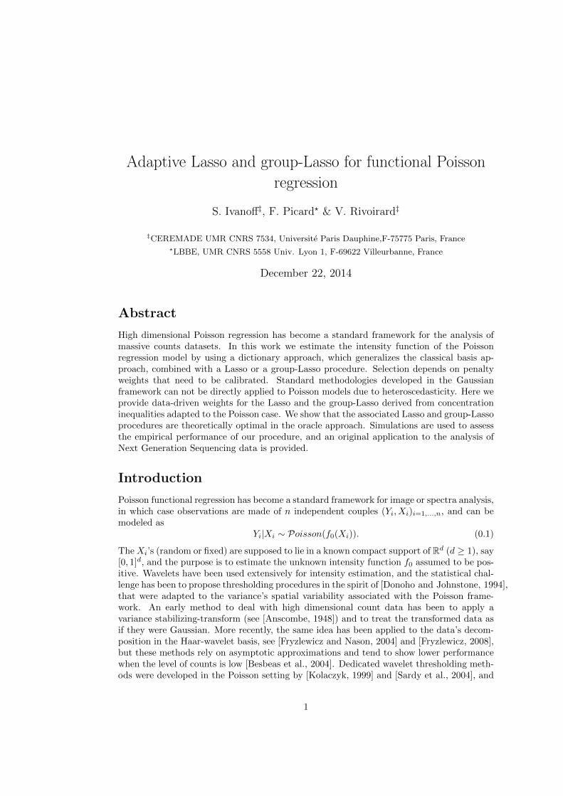
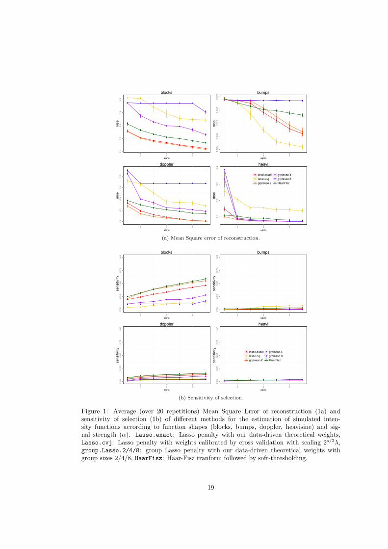
Performance measurement. For any estimate f , reconstruction performance were mea-sured using the (normalized) mean-squared error MSE = ‖f − f0‖22/‖f0‖22 (Figure 1a), andselection performance were measured by the standard indicators: accuracy on support re-covery, sensitivity (proportion of true non-null coefficients among selected coefficients) andspecificity of detection (proportion of true null coefficients among non-selected coefficients),

based on the estimated support of β and on the support of β0, the coefficients associatedwith the projection of function f0 on the dictionary.

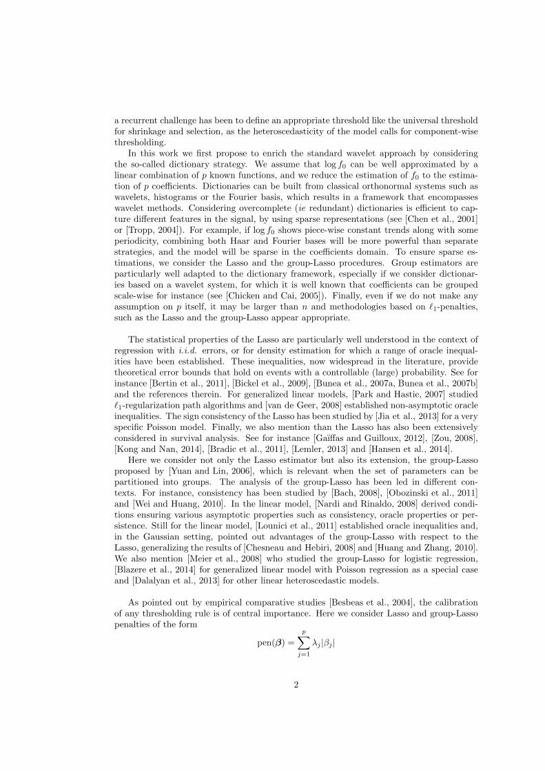
Performance in the basis setting. The first step of our simulation study relies onwavelet basis (Haar or Daubechies) and not on a dictionary approach (considered in asecond step) in order to compare our calibrated weights with other methods that rely onpenalized strategy. It appears that, except for the bumps function, the Lasso with exactweights shows the lowest reconstruction error whatever the shape of the intensity function(Figure 1a). Moreover, better performance of the Lasso with exact weights in cases of lowintensity emphasize the interest of theoretically calibrated procedures rather than asymp-totic approximations (like the Haar-Fisz transform). In the case of bumps, cross-validationseems to perform better than the Lasso, but when looking at reconstructed average function(Figure 2a) this lower reconstruction error of cross-validation is associated with higher localvariations around the peaks. Compared with Haar-Fisz, the gain of using exact weights issubstantial even when the signal to noise ratio is high, which indicates that even in the va-lidity domain of the Haar-Fisz transform (large intensities), the Lasso combined with exactthresholds is more suitable (Figure 2a). As for the group Lasso, its performance highly de-pend on the group size: while groups of size 2 show similar performance as the Lasso, groupsof size 4 and 8 increase the reconstruction error (Figure 1a and 2b), since they are not scaledto the size of the irregularities in the signal. This trend is not systematic as the group Lassoappears to be adapted to functions that are more regular (Heavisine), and seems to avoidedge effects in some situations. Very interestingly, the group Lasso of size 2 increases thesensitivity of detection for the Lasso (Figure 1b), while keeping the same specificity, whichsuggests that it accounts for (true) local variations of nearby coefficients, which results ina slightly better reconstruction error. As a last remark we mention that the sensitivitiesof all methods are rather low regarding coefficients selection, meaning that many true nonnull coefficients remain unselected. Since reconstruction errors are satisfactory, this meansthat only few coefficients needed to be selected for good reconstruction properties in thefunctional domain.

17

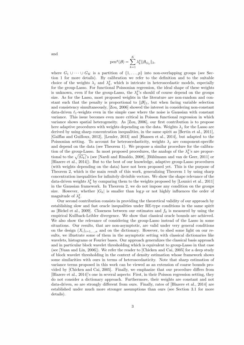
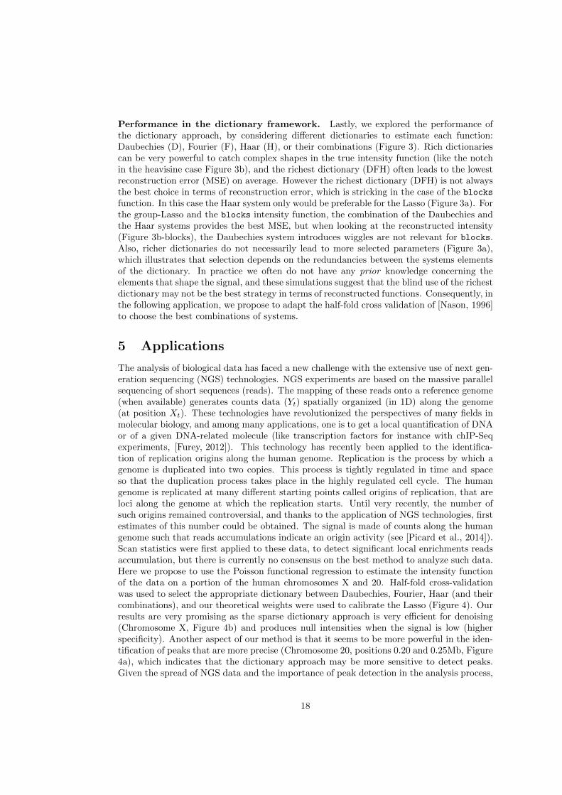
Performance in the dictionary framework. Lastly, we explored the performance ofthe dictionary approach, by considering different dictionaries to estimate each function:Daubechies (D), Fourier (F), Haar (H), or their combinations (Figure 3). Rich dictionariescan be very powerful to catch complex shapes in the true intensity function (like the notchin the heavisine case Figure 3b), and the richest dictionary (DFH) often leads to the lowestreconstruction error (MSE) on average. However the richest dictionary (DFH) is not alwaysthe best choice in terms of reconstruction error, which is stricking in the case of the blocks

function. In this case the Haar system only would be preferable for the Lasso (Figure 3a). Forthe group-Lasso and the blocks intensity function, the combination of the Daubechies andthe Haar systems provides the best MSE, but when looking at the reconstructed intensity(Figure 3b-blocks), the Daubechies system introduces wiggles are not relevant for blocks.Also, richer dictionaries do not necessarily lead to more selected parameters (Figure 3a),which illustrates that selection depends on the redundancies between the systems elementsof the dictionary. In practice we often do not have any prior knowledge concerning theelements that shape the signal, and these simulations suggest that the blind use of the richestdictionary may not be the best strategy in terms of reconstructed functions. Consequently, inthe following application, we propose to adapt the half-fold cross validation of [Nason, 1996]to choose the best combinations of systems.

5 Applications

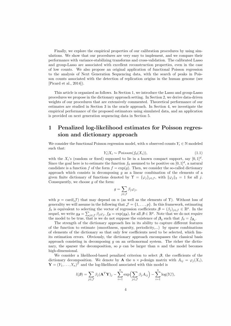
The analysis of biological data has faced a new challenge with the extensive use of next gen-eration sequencing (NGS) technologies. NGS experiments are based on the massive parallelsequencing of short sequences (reads). The mapping of these reads onto a reference genome(when available) generates counts data (Yt) spatially organized (in 1D) along the genome(at position Xt). These technologies have revolutionized the perspectives of many fields inmolecular biology, and among many applications, one is to get a local quantification of DNAor of a given DNA-related molecule (like transcription factors for instance with chIP-Seqexperiments, [Furey, 2012]). This technology has recently been applied to the identifica-tion of replication origins along the human genome. Replication is the process by which agenome is duplicated into two copies. This process is tightly regulated in time and spaceso that the duplication process takes place in the highly regulated cell cycle. The humangenome is replicated at many different starting points called origins of replication, that areloci along the genome at which the replication starts. Until very recently, the number ofsuch origins remained controversial, and thanks to the application of NGS technologies, firstestimates of this number could be obtained. The signal is made of counts along the humangenome such that reads accumulations indicate an origin activity (see [Picard et al., 2014]).Scan statistics were first applied to these data, to detect significant local enrichments readsaccumulation, but there is currently no consensus on the best method to analyze such data.Here we propose to use the Poisson functional regression to estimate the intensity functionof the data on a portion of the human chromosomes X and 20. Half-fold cross-validationwas used to select the appropriate dictionary between Daubechies, Fourier, Haar (and theircombinations), and our theoretical weights were used to calibrate the Lasso (Figure 4). Ourresults are very promising as the sparse dictionary approach is very efficient for denoising(Chromosome X, Figure 4b) and produces null intensities when the signal is low (higherspecificity). Another aspect of our method is that it seems to be more powerful in the iden-tification of peaks that are more precise (Chromosome 20, positions 0.20 and 0.25Mb, Figure4a), which indicates that the dictionary approach may be more sensitive to detect peaks.Given the spread of NGS data and the importance of peak detection in the analysis process,

18

0.1

0.2

0.3

0.4

0.5

2 4 6alpha

mse

blocks

0.22

50.

250

0.27

50.

300

0.32

5

2 4 6alpha

mse

bumps

0.1

0.2

0.3

0.4

0.5

2 4 6alpha

mse

doppler

0.1

0.2

0.3

0.4

2 4 6alpha

mse

lasso.exactlasso.cvjgrplasso.2

grplasso.4grplasso.8HaarFisz

heavi

(a) Mean Square error of reconstruction.

0.00

0.25

0.50

0.75

1.00

2 4 6alpha

sens

itivi

ty

blocks

0.00

0.25

0.50

0.75

1.00

2 4 6alpha

sens

itivi

ty

bumps

0.00

0.25

0.50

0.75

1.00

2 4 6alpha

sens

itivi

ty

doppler

0.00

0.25

0.50

0.75

1.00

2 4 6alpha

sens

itivi

ty

lasso.exactlasso.cvjgrplasso.2

grplasso.4grplasso.8HaarFisz

heavi

(b) Sensitivity of selection.

Figure 1: Average (over 20 repetitions) Mean Square Error of reconstruction (1a) andsensitivity of selection (1b) of different methods for the estimation of simulated inten-sity functions according to function shapes (blocks, bumps, doppler, heavisine) and sig-nal strength (α). Lasso.exact: Lasso penalty with our data-driven theoretical weights,Lasso.cvj: Lasso penalty with weights calibrated by cross validation with scaling 2s/2λ,group.Lasso.2/4/8: group Lasso penalty with our data-driven theoretical weights withgroup sizes 2/4/8, HaarFisz: Haar-Fisz tranform followed by soft-thresholding.

19

010

2030

0.00 0.25 0.50 0.75 1.00

blocks

510

1520

25

0.00 0.25 0.50 0.75 1.00

bumps

05

1015

2025

0.00 0.25 0.50 0.75 1.00

doppler

010

20

0.00 0.25 0.50 0.75 1.00

lasso.exactlasso.cvjHaarFiszf0

heavi

(a) Average reconstructed functions for the Lasso and competitors.

010

2030

0.00 0.25 0.50 0.75 1.00

blocks

510

1520

25

0.00 0.25 0.50 0.75 1.00

bumps

05

1015

2025

0.00 0.25 0.50 0.75 1.00

doppler

010

20

0.00 0.25 0.50 0.75 1.00

lasso.exactgrplasso.2grplasso.4grplasso.8f0

heavi

(b) Average reconstructed functions for the group strategies.

Figure 2: Average (over 20 repetitions) reconstructed functions by different methods ofestimation according to function shapes (blocks, bumps, doppler, heavisine). Top panelcorresponds to non-grouped strategies (2a) and bottom panel compares group-strategiesto the Lasso (2b). Lasso.exact: Lasso penalty with our data-driven theoretical weights,Lasso.cvj: Lasso penalty with weights calibrated by cross validation with scaling 2s/2λ,group.Lasso.2/4/8: group Lasso penalty with our data-driven theoretical weights withgroup sizes 2/4/8, HaarFisz: Haar-Fisz tranform followed by soft-thresholding, f0: simu-lated intensity function. 20

D

DF

DFHDH

F

FHH

HD

DF

DFHDH

F

FH

H

0.15

0.16

0.17

0.18

0.19

25 35 45 55 65df

MSE

aaa

grplasso.2HaarFiszlasso

blocks

D

DFDFH

DH

F

FH

H

D

DDFDFHDH

F

FHH

0.26

0.27

0.28

0.29

0.30

0.31

5.0 7.5 10.0 12.5df

MSE

aaa

grplasso.2HaarFiszlasso

bumps

DDF DFH

DH

F

FH

H

D

DDF

DFH

DH

F

FH

H

0.12

50.

150

0.17

5

30 40 50df

MSE

aaa

grplasso.2HaarFiszlasso

doppler

DDF

DFH

DHFFH

H

D

DDF

DFH

DHF

FH

H

0.07

0.09

0.11

0.13

7.5 10.0 12.5 15.0df

MSE

aaa

grplasso.2HaarFiszlasso

heavi

(a) Average Mean Square Error for different dictionaries with respect to the average number ofselected coefficients (df).

010

2030

0.00 0.25 0.50 0.75 1.00

grplasso.2 + DHHaarFisz + Hlasso + Htruth

blocks

510

1520

25

0.00 0.25 0.50 0.75 1.00

grplasso.2 + DFHHaarFisz + Dlasso + Dtruth

bumps

05

1015

20

0.00 0.25 0.50 0.75 1.00

grplasso.2 + DFHHaarFisz + Dlasso + Dtruth

doppler

05

1015

2025

0.00 0.25 0.50 0.75 1.00

grplasso.2 + DFHHaarFisz + Dlasso + DFHtruth

heavi

(b) Reconstructed functions for the dictionaries with the smallest MSE.

Figure 3: Average (over 20 repetitions) Mean Square Errors and number of selected co-efficients (df) (3a), and reconstructed functions (3b) for different dictionaries: Daubechies(D), Fourier (F), Haar (H) and their combinations. Lasso.exact: Lasso penalty withour data-driven theoretical weights, group.Lasso.2: group Lasso penalty with our data-driven theoretical weights with group sizes 2, HaarFisz: Haar-Fisz tranform followed bysoft-thresholding. 21

for chIP-Seq [Furey, 2012], FAIRE-Seq [Thurman et al., 2012], OriSeq [Picard et al., 2014],our preliminary results suggest that the sparse dictionary approach will be a very promisingframework for the analysis of such data.

22

0.00 0.05 0.10 0.15 0.20 0.25

02

46

810

12

Genomic Location (Mb)

Num

ber o

f rea

ds

(a) Chromosome 20

2.75 2.80 2.85 2.90 2.95

05

1015

2025

30

Genomic Location (Mb)

Num

ber o

f rea

ds

(b) Chromosome X

Figure 4: Estimation of the intensity function of Ori-Seq data (chromosomes 20 4a andX 4b). Grey bars indicate the number of reads that match genomic positions (x-axis, inMegaBases). The red line corresponds to the estimated intensity function, and verticaldotted lines stand for the detected origins by scanning statistics.

23

6 Proofs

6.1 Proof of Theorem 1

We denote by µ the Lebesgue measure on Rd and we introduce a partition of the set [0, 1]d

denoted ∪ni=1Si so that for any i = 1, . . . , n, Xi ∈ Si and µ(Si) > 0. Let h the functiondefined for any t ∈ [0, 1]d by

h(t) =

n∑i=1

f0(Xi)

µ(Si)1Si(t).

Finally, we introduce N the Poisson process on [0, 1]d with intensity h (see [Kingman, 1993]).Therefore, for any i = 1, . . . , n, N(Si) is a Poisson variable with parameter

∫Sih(t)dt =

f0(Xi) and since ∪ni=1Si is a partition of [0, 1]d, (N(S1), . . . , N(Sn)) has the same distributionas (Y1, . . . , Yn). We observe that if for any j = 1, . . . , p,

ϕj(t) =

n∑i=1

ϕj(Xi)1Si(t),

then ∫ϕj(t)dN(t) ∼

n∑i=1

ϕj(Xi)Yi = ATj Y.

We use the following exponential inequality (see Inequality (5.2) of [Reynaud-Bouret, 2003]).If g is bounded, for any u > 0,

P

(∫g(x)(dN(x)− h(x)dx) ≥

√2u

∫g2(x)h(x)dx+

u

3||g||∞

)≤ exp(−u). (6.1)

By taking successively g = ϕj and g = −ϕj , we obtain

P

(|AT

j (Y − E[Y])| ≥

√2u

∫ϕ2j (x)h(x)dx+

u

3‖ϕj‖∞

)≤ 2e−u.

Since ∫ϕ2j (x)h(x)dx =

n∑i=1

ϕ2j (Xi)f0(Xi) = Vj ,

we obtain

P

(|AT

j (Y − E[Y])| ≥√

2uVj +u

3‖ϕj‖∞

)≤ 2e−u. (6.2)

To control Vj , we use (6.1) with g = −ϕ2j and we have:

P

(Vj − Vj ≥

√2u

∫ϕ4j (t)h(t)dt+

u

3‖ϕj‖2∞

)≤ e−u.

We observe that ∫ϕ4j (t)h(t)dt ≤ ‖ϕj‖2∞

∫ϕ2j (t)h(t)dt = ‖ϕj‖2∞Vj .

24

Setting vj = u‖ϕj‖2∞, we have:

P

(Vj −

√2vjVj −

vj3− Vj ≥ 0

)≤ e−u.

Let αj =√Vj + 5

6vj+√

vj2 , such that αj is the positive solution to α2

j−√

2vjαj−(Vj+vj3 ) =

0. ThenP(Vj ≥ α2

j

)= P

(√Vj ≥ αj

)≤ e−u. (6.3)

We choose u = γ log p and observe that α2j ≤ Vj . Then, by combining (6.2) and (6.3), we

have

P

(|AT

j (Y − E[Y])| ≥√

2γ log pVj +γ log p

3‖ϕj‖∞

)≤ 3

pγ.

As ‖ϕj‖∞ = maxi |ϕj(Xi)|, the theorem follows.

Remark 2. By slightly extending previous computations, we easily show that for u > 0,

P

(|Vj − Vj | ≥

√2uVj‖ϕj‖2∞ +

u

3‖ϕj‖2∞

)≤ 2e−u,

which leads to

P

(|Vj − Vj | ≥

Vj2

+4γ log p

3‖ϕj‖2∞

)≤ 2

pγ.

6.2 Proof of Theorem 2

For each k ∈ 1, . . . ,K, we recall that bik =√∑

j∈Gk ϕ2j (Xi), so bik = ‖AT

Gkei‖2, where

ei is the vector whose i-th coordinate is equal to 1 and all others to 0. We first state thefollowing lemma:

Lemma 1. Let k be fixed. Assume that there exists some M > 0 such that ∀x, |f0(x)| ≤M .Assume further that there exists some ck ≥ 0 such that ∀y ∈ Rn, ‖AGkA

TGk

y‖2 ≤ ck‖ATGk

y‖2.Then, ∀x > 0,∀ ε > 0,

P

(‖AT

Gk(Y − E[Y])‖2 ≥ (1 + ε)

√∑j∈Gk

Vj + x

)≤ exp

(x

bk−( xbk

+Dεk

b2k

)log(

1 +bkx

Dεk

)),

where Dεk = 8Mc2k + 2

ε2 b2k.

Proof. With k ∈ 1, . . . ,K being fixed, we define f : Rn → R by f(y) =(‖AT

Gky‖2−E

)+

,

where E > 0 is a constant chosen later. We use Corollary 1 from [Houdre et al., 2008],applied to the infinitely divisible vector Y−E[Y] ∈ Rn, whose components are independent,and to f . First note that for any t > 0,

Eetbik|Yi−EYi| ≤ Eetb

ik(Yi+f0(Xi))

= exp(f0(Xi)(e

tbik + tbik − 1))<∞.

25

Furthermore, for any i ∈ 1, ..., n, any y ∈ Rn and any u ∈ R,

|f(y + uei)− f(y)| ≤∣∣∣‖AT

Gk(y + uei)‖2 − ‖AT

Gky‖2∣∣∣

≤ ‖ATGk

(uei)‖2= |u|bik.

Therefore, for all x > 0,

P(f(Y − E[Y])− E[f(Y − E[Y])] ≥ x

)≤ exp

(−∫ x

0

h−1f (s)ds

),

where hf is defined for all t > 0 by

hf (t) = supy∈Rn

n∑i=1

∫R|f(y + uei)− f(y)|2 e

tbik|u| − 1

bik|u|νi(du)

and νi is the Levy measure associated with Yi−E[Yi]. It is easy to show that νi = f0(Xi)δ1,and so

hf (t) = supy∈Rn

n∑i=1

f0(Xi)(f(y + ei)− f(y)

)2 etbik − 1

bik.

Furthermore, writing Ai =‖AT

Gk(y + ei)‖2 ≥ E or ‖AT

Gky‖2 ≥ E

, we have

|f(y + ei)− f(y)| ≤∣∣∣‖AT

Gk(y + ei)‖2 − ‖AT

Gky‖2∣∣∣1Ai

=1Ai

∣∣∣‖ATGk

(y + ei)‖22 − ‖ATGk

y‖22∣∣∣

‖ATGk

(y + ei)‖2 + ‖ATGk

y‖2

=1Ai

∣∣∣2 < ATGk

ei,ATGk

y > +‖ATGk

ei‖22∣∣∣

‖ATGk

(y + ei)‖2 + ‖ATGk

y‖2

≤ 2

∣∣∣ < ATGk

ei,ATGk

y >∣∣∣

‖ATGk

y‖2+‖AT

Gkei‖22

E,

with < ·, · > the usual scalar product. We now have(f(y + ei)− f(y)

)2

≤ 8< AT

Gkei,A

TGk

y >2

‖ATGk

y‖22+ 2‖AT

Gkei‖42

E2.

The first term can be rewritten as 8<ei,AGk

ATGk

y>2

‖ATGk

y‖22and the second one is equal to 2

bik4

E2 , so

we can now bound hf (t) as follows.

hf (t) ≤ supy

∑i

f0(Xi)etb

ik − 1

bik

(8< ei,AGkA

TGk

y >2

‖ATGk

y‖22+ 2

bik4

E2

)

≤ etbk − 1

bksupy

(8M‖AGkA

TGk

y‖22‖AT

Gky‖22

+2

E2

∑i

f0(Xi)bik

4

)

≤ etbk − 1

bk

(8Mc2k +

2

E2

∑i

f0(Xi)bik

4

).

26

Now, we set

E = ε

√∑j∈Gk

Vj .

So we have:

E2 = ε2∑j∈Gk

n∑i=1

f0(Xi)ϕ2j (Xi)

= ε2n∑i=1

f0(Xi)∑j∈Gk

ϕ2j (Xi)

= ε2n∑i=1

f0(Xi)bik

2.

Thus, we can finally bound the function hf by the increasing function h defined by

h(t) = Dεk

etbk − 1

bk,

with Dεk = 8Mc2k +

2b2kε2 . Therefore,

exp(−∫ x

0

h−1f (s)ds

)≤ exp

(−∫ x

0

h−1(s)ds)

= exp

(x

bk−( xbk

+Dεk

b2k

)log(

1 +bkx

Dεk

)).

Now,

f(Y − E[Y])− E[f(Y − E[Y])] =(‖AT

Gk(Y − E[Y])‖2 − E

)+− E

(‖AT

Gk(Y − E[Y])‖2 − E

)+

≥ ‖ATGk

(Y − E[Y])‖2 − E − E‖ATGk

(Y − E[Y])‖2.

Furthermore, by Jensen’s inequality, we have

E‖ATGk

(Y − E[Y])‖2 ≤√

E‖ATGk

(Y − E[Y])‖22

=

√∑j∈Gk

E[(ATj (Y − EY))2]

=

√∑j∈Gk

Var(ATj Y)

=

√∑j∈Gk

Vj .

Recalling that E = ε√∑

j∈Gk Vj , we thus have

P(f(Y − E[Y])− Ef(Y − E[Y]) ≥ x

)≥ P

(‖AT

Gk(Y − E[Y])‖2 − (1 + ε)

√∑j∈Gk

Vj ≥ x),

27

which concludes the proof. We apply Lemma 1 with

ε =1

2√

2γ log pand x = 2

√γ log pDε

k.

Then,

bkx

Dεk

=2bk√γ log p√Dεk

=2bk√γ log p√

8Mc2k +2b2kε2

≤ ε√

2γ log p =1

2.

Finally, using the fact that log(1 + u) ≥ u− u2

2 , we have:

exp

(x

bk−( xbk

+Dεk

b2k

)log(

1 +bkx

Dεk

))≤ exp

(x

bk−( xbk

+Dεk

b2k

)(bkxDεk

− b2kx2

2Dεk

2

))

= exp

(−x2

2Dεk

+bkx

3

2Dεk

2

)

= exp

(−x2

2Dεk

(1− bkx

Dεk

))

≤ exp(−x2

4Dεk

)=

1

pγ.

We obtain

P

(‖AT

Gk(Y − E[Y])‖2 ≥ (1 + ε)

√∑j∈Gk

Vj + 2√γ log pDε

k

)≤ 1

pγ.

We control Vj as in the proof of Theorem 1, but we take u = γ log p+ log |Gk|. The analogof (6.3) is

P(Vj > V gj

)≤ e−u =

1

|Gk|pγ

and thus

P(∃ j ∈ Gk, Vj > V gj

)≤ 1

pγ.

This concludes the proof of Theorem 2.

6.3 Proof of Proposition 1

For the first point, we write:

‖AGkATGk

x‖22 =

n∑l=1

( ∑j∈Gk

ϕj(Xl)

n∑i=1

ϕj(Xi)xi

)2

.

28

Then, we apply the Cauchy-Schwarz inequality:

‖AGkATGk

x‖22 ≤n∑l=1

( ∑j∈Gk

ϕ2j (Xl)

)( ∑j∈Gk

( n∑i=1

ϕj(Xi)xi

)2)

= ‖ATGk

x‖22n∑l=1

( ∑j∈Gk

ϕ2j (Xl)

)

= ‖ATGk

x‖22n∑l=1

(blk)2

≤ nb2k‖ATGk

x‖22,

which proves the upper bound of (2.11). For the lower bound, we just observe that for anyi = 1, . . . , n, with ei the vector whose i-th coordinate is equal to 1 and all others to 0,

bik2

= ‖ATGk

ei‖22= < AT

Gkei,A

TGk

ei >

= < ei,AGkATGk

ei >

≤ ‖ei‖2‖AGkATGk

ei‖2≤ ck‖AT

Gkei‖2

= ckbik,

which obviously entails bk ≤ ck. For the last point, we observe that

‖ATGk

x‖22 =∑j∈Gk

K2j ,

where Kj =∑ni=1 ϕj(Xi)xi. By expressing ‖AGkA

TGk

x‖22 with respect to the Kj ’s, weobtain:

‖AGkATGk

x‖22 =

n∑l=1

( ∑j∈Gk

ϕj(Xl)

n∑i=1

ϕj(Xi)xi

)2

=

n∑l=1

∑j∈Gk

ϕj(Xl)

n∑i=1

ϕj(Xi)xi∑j′∈Gk

ϕj′(Xl)

n∑i′=1

ϕj′(Xi′)xi′

=∑j∈Gk

∑j′∈Gk

n∑l=1

ϕj(Xl)ϕj′(Xl)

n∑i=1

ϕj(Xi)xi

n∑i′=1

ϕj′(Xi′)xi′

=∑j∈Gk

∑j′∈Gk

n∑l=1

ϕj(Xl)ϕj′(Xl)KjKj′

≤ 1

2

∑j∈Gk

∑j′∈Gk

∣∣∣ n∑l=1

ϕj(Xl)ϕj′(Xl)∣∣∣(K2

j +K2j′)

=∑j∈Gk

∑j′∈Gk

∣∣∣ n∑l=1

ϕj(Xl)ϕj′(Xl)∣∣∣K2

j ,

from which we deduce (2.12).

29

6.4 Proof of Theorem 3

For any β ∈ Rp, we have

K(f0, fβ) =

n∑i=1

f0(Xi)(

log f0(Xi)− log fβ(Xi))

+ fβ(Xi)− f0(Xi)

=

n∑i=1

Yi(

log f0(Xi)− log fβ(Xi))

+ fβ(Xi)− f0(Xi)

+

n∑i=1

(f0(Xi)− Yi)(

log f0(Xi)− log fβ(Xi))

= logL(f0)− logL(fβ) +

n∑i=1

(f0(Xi)− Yi)(

log f0(Xi)− log fβ(Xi)).

Therefore, for all β ∈ Rp,

K(f0, fgL)−K(f0, fβ) = l(β)− l(β

gL) +

n∑i=1

(f0(Xi)− Yi

)(log fβ(Xi)− log fgL(Xi)

)= l(β)− l(β

gL) +

n∑i=1

(f0(Xi)− Yi

) p∑j=1

(βj − βgLj )ϕj(Xi)

= l(β)− l(βgL

) +

p∑j=1

(βgLj − βj)n∑i=1

ϕj(Xi)(Yi − f0(Xi)).

Let us write ηj =∑ni=1 ϕj(Xi)(Yi − f0(Xi)) = AT

j (Y − E[Y]). We have

K(f0, fgL) = K(f0, fβ) + l(β)− l(β

gL) + (β

gL− β)Tη. (6.4)

By definition of βgL

,

−l(βgL

) +

K∑k=1

λgk‖βgL

Gk‖2 ≤ −l(β) +

K∑k=1

λgk‖βGk‖2.

Furthermore, on Ωg,

|(βgL− β)Tη| =

∣∣∣ p∑j=1

(βgLj − βj)(ATj (Y − EY))

∣∣∣≤

K∑k=1

∑j∈Gk

|βgLj − βj ||ATj (Y − EY)|

≤K∑k=1

( ∑j∈Gk

(βgLj − βj)2)1/2( ∑

j∈Gk

(ATj (Y − EY))2

)1/2

=

K∑k=1

‖βgL

Gk− βGk‖2‖A

TGk

(Y − EY)‖2

≤K∑k=1

λgk‖βgL

Gk− βGk‖2. (6.5)

30

Therefore, for all β ∈ Rp,

K(f0, fgL) ≤ K(f0, fβ) +

K∑k=1

λgk

(‖β

gL

Gk− βGk‖2 − ‖β

gL

Gk‖2 + ‖βGk‖2

),

from which we deduce (3.3).

6.5 Proof of Theorem 4

We start from Equality (6.4) combined with Inequality (6.5). Then, we have that on Ωg, forany β,

K(f0, fgL)+(α−1)

K∑k=1

λgk‖βgL

Gk−βGk‖2 ≤ K(f0, fβ)+

K∑k=1

αλgk

(‖β

gL

Gk−βGk‖2−‖β

gL

Gk‖2+‖βGk‖2

).

On J(β)c, ‖βgL

Gk− βGk‖2 − ‖β

gL

Gk‖2 + ‖βGk‖2 = 0 and

K(f0, fgL) + (α− 1)

K∑k=1

λgk‖βgL

Gk− βGk‖2 ≤ K(f0, fβ) + 2α

∑k∈J(β)

λgk‖βgL

Gk− βGk‖2. (6.6)

By applying the Cauchy-Schwarz inequality we also have

K(f0, fgL)+(α−1)

K∑k=1

λgk‖βgL

Gk−βGk‖2 ≤ K(f0, fβ)+2α|J(β)|1/2

( ∑k∈J(β)

(λgk)2‖βgL

Gk−βGk‖

22

)1/2

.

(6.7)

If we write ∆ = D(βgL− β), where D is a diagonal matrix with Dj,j = λgk if j ∈ Gk, then

we can rewrite (6.6) as

K(f0, fgL) + (α− 1)‖∆‖1,2 ≤ K(f0, fβ) + 2α‖∆J(β)‖1,2 (6.8)

and we deduce from (6.7)

K(f0, fgL) ≤ K(f0, fβ) + 2α(|J(β)|)1/2‖∆J(β)‖2. (6.9)

Now, on the event

2α‖∆J(β)‖1,2 ≤ εK(f0, fβ)

, the theorem follows immediately from(6.8). We now assume that εK(f0, fβ) ≤ 2α‖∆J(β)‖1,2. Since K is non-negative, we deducefrom (6.8) that

(α− 1)‖∆‖1,2 ≤ 2α(

1 +1

ε

)‖∆J(β)‖1,2,

(α− 1)‖∆J(β)c‖1,2 ≤

(2α(

1 +1

ε

)− (α− 1)

)‖∆J(β)‖1,2

and

‖∆J(β)c‖1,2 ≤

(α+ 1 + 2α/ε

α− 1

)‖∆J(β)‖1,2.

This yields the following inequality for the vector D−1∆ = (βgL− β):

‖(βgL− β)J(β)c‖1,2 ≤

maxk λgk

mink λgk

α+ 1 + 2α/ε

α− 1‖(β

gL− β)J(β)‖1,2.

31

From Assumption 2 we have that, if β is such that |J(β)| ≤ s, then

‖(βgL− β)J(β)‖2 ≤

1

κn

((β

gL− β)TG(β

gL− β)

)1/2.

Since

Gj,j′ =

n∑i=1

ϕj(Xi)ϕj′(Xi)f0(Xi),

by setting

ui = log fβ(Xi)− log f0(Xi) and ugLi = log fβgL(Xi)− log f0(Xi),

we have

(βgL− β)TG(β

gL− β) =

p∑j=1

p∑j′=1

(βgLj − βj)(βgLj′ − βj′)Gj,j′

=

n∑i=1

f0(Xi)( p∑j=1

(βgLj − βj)ϕj(Xi))2

=

n∑i=1

f0(Xi)(ugLi − ui)

2.

We set h(f0, fβ) =∑ni=1 f0(Xi)u

2i and h(f0, f

gL) =∑ni=1 f0(Xi)(u

gLi )2. From (6.9) and

since

‖∆J(β)‖2 ≤ (maxk

λgk)‖(βgL− β)J(β)‖2

≤maxk λ

gk

κn

((β

gL− β)TG(β

gL− β)

)1/2,

we have

K(f0, fgL) ≤ K(f0, fβ) +

2α

κn|J(β)|1/2(max

kλgk)(√

h(f0, fgL) +√h(f0, fβ)

).

To conclude, we use arguments similar to [Lemler, 2013]. We recall them for the safe ofcompleteness. To connect h(f0, fβ) to K(f0, fβ), we use Lemma 1 of [Bach, 2010] that isrecalled now.

Lemma 2. Let g be a convex three times differentiable function g : R→ R such that for allt ∈ R, |g′′′(t)| ≤ Sg′′(t) for some S ≥ 0. Then, for all t ≥ 0,

g′′(0)

S2φ(−St) ≤ g(t)− g(0)− g′(0)t ≤ g′′(0)

S2φ(St),

where φ(x) = ex − x− 1.

Let h be a real function. We set

G(h) =

n∑i=1

(eh(Xi) − f0(Xi)h(Xi)

)

32

andg(t) = G(h+ tk),

where h and k are functions and t ∈ R. We have :

g′(t) =

n∑i=1

(k(Xi)e

h(Xi)+tk(Xi) − f0(Xi)k(Xi)),

g′′(t) =

n∑i=1

(k2(Xi)e

h(Xi)+tk(Xi))

and

g′′′(t) =

n∑i=1

(k3(Xi)e

h(Xi)+tk(Xi)).

Therefore |g′′′(t)| ≤ Sg′′(t) with S = maxi |k(Xi)|. We choose h(Xi) = log f0(Xi) andk(Xi) = ui = log fβ(Xi)− log f0(Xi) and we apply Lemma 2 to g with t = 1. Computationsyield that g(1) − g(0) = K(f0, fβ), g′(0) = 0 and g′′(0) =

∑ni=1 f0(Xi)u

2i = h(f0, fβ).

Thereforeφ(−S)

S2h(f0, fβ) ≤ K(f0, fβ) ≤ φ(S)

S2h(f0, fβ).

Finally, using Assumption 1, for β ∈ Γ(µ), S = maxi |ui| ≤ µ. Furthermore, x −→ φ(x)x2 is a

nonnegative increasing function and therefore we have

µ′h(f0, fβ) ≤ K(f0, fβ) ≤ µ′′h(f0, fβ),

where µ′ = φ(−µ)µ2 and µ′′ = φ(µ)

µ2 . It follows that, for β ∈ Γ(µ),

K(f0, fgL) ≤ K(f0, fβ) +

2α

κn√µ′|J(β)|1/2(max

kλgk)(√

K(f0, fgL) +√K(f0, fβ)

).

We use twice the inequality 2uv ≤ bu2+ v2

b for any b > 0, applied to u = ακn

√|J(β)|(maxk λ

gk)

and v being either√

1µ′K(f0, fgL) or

√1µ′K(f0, fβ). We have

(1− 1

µ′b

)K(f0, f

gL) ≤(

1 +1

µ′b

)K(f0, fβ) + 2b

α2|J(β)|κ2n

(maxk

λgk)2.

Finally,

K(f0, fgL) ≤

(µ′b+ 1

µ′b− 1

)K(f0, fβ) + 2

µ′b2

µ′b− 1

α2|J(β)|κ2n

(maxk

λgk)2.

We choose b > 1/µ′ such that µ′b+1µ′b−1 = 1 + ε and we set B(ε, µ) = 2(1 + ε)−1 µ′b2

µ′b−1 . Finally,

we have, for any β ∈ Γ(µ) such that |J(β)| ≤ s,

K(f0, fgL) ≤ (1 + ε)

(K(f0, fβ) +B(ε, µ)

α2|J(β)|κ2n

(maxk

λgk)2

).

This completes the proof of Theorem 4.

Acknowledgements: The research of Stephane Ivanoff and Vincent Rivoirard is partlysupported by the french Agence Nationale de la Recherche (ANR 2011 BS01 010 01 projetCalibration). The research of Franck Picard is partly supported by the ABS4NGS ANRproject ANR-11-BINF-0001-06.

33

References

[Anscombe, 1948] Anscombe, F. J. (1948). The transformation of Poisson, binomial andnegative-binomial data. Biometrika, 35:246–254.

[Bach, 2010] Bach, F. (2010). Self-concordant analysis for logistic regression. Electron. J.Stat., 4:384–414.

[Bach, 2008] Bach, F. R. (2008). Consistency of the group lasso and multiple kernel learning.J. Mach. Learn. Res., 9:1179–1225.

[Bertin et al., 2011] Bertin, K., Le Pennec, E., and Rivoirard, V. (2011). Adaptive Dantzigdensity estimation. Ann. Inst. Henri Poincare Probab. Stat., 47(1):43–74.

[Besbeas et al., 2004] Besbeas, P., De Feis, I., and Sapatinas, T. (2004). A comparative sim-ulation study of wavelet shrinkage estimators for Poisson counts. Intern. Statist. Review,72(2):209–237.

[Bickel et al., 2009] Bickel, P. J., Ritov, Y., and Tsybakov, A. B. (2009). Simultaneousanalysis of lasso and Dantzig selector. Ann. Statist., 37(4):1705–1732.

[Blazere et al., 2014] Blazere, M., Loubes, J.-M., and Gamboa, F. (2014). Oracle inequalitiesfor a group lasso procedure applied to generalized linear models in high dimension. IEEETransactions on Information Theory, 4(12):2303–2318.

[Bradic et al., 2011] Bradic, J., Fan, J., and Jiang, J. (2011). Regularization for Cox’sproportional hazards model with NP-dimensionality. Ann. Statist., 39(6):3092–3120.

[Buhlmann and van de Geer, 2011] Buhlmann, P. and van de Geer, S. (2011). Statisticsfor high-dimensional data. Springer Series in Statistics. Springer, Heidelberg. Methods,theory and applications.

[Bunea et al., 2007a] Bunea, F., Tsybakov, A., and Wegkamp, M. (2007a). Sparsity oracleinequalities for the Lasso. Electron. J. Stat., 1:169–194.

[Bunea et al., 2007b] Bunea, F., Tsybakov, A. B., and Wegkamp, M. H. (2007b). Aggrega-tion for Gaussian regression. Ann. Statist., 35(4):1674–1697.

[Chen et al., 2001] Chen, S. S., Donoho, D. L., and Saunders, M. A. (2001). Atomic de-composition by basis pursuit. SIAM Rev., 43(1):129–159. Reprinted from SIAM J. Sci.Comput. 20 (1998), no. 1, 33–61 (electronic) [ MR1639094 (99h:94013)].

[Chesneau and Hebiri, 2008] Chesneau, C. and Hebiri, M. (2008). Some theoretical resultson the grouped variables Lasso. Math. Methods Statist., 17(4):317–326.

[Chicken and Cai, 2005] Chicken, E. and Cai, T. (2005). Block thresholding for densityestimation: Local and global adaptivity. Journal of Multivariate Analysis, 95:76–106.

[Dalalyan et al., 2013] Dalalyan, A. S., Hebiri, M., Meziani, K., and Salmon, J. (2013).Learning heteroscedastic models by convex programming under group sparsity. In ICML.

[Donoho and Johnstone, 1994] Donoho, D. and Johnstone, I. (1994). Ideal spatial adapta-tion by wavelet shrinkage. Biometrika, 81:425–455.

[Fryzlewicz, 2008] Fryzlewicz, P. (2008). Data-driven wavelet-Fisz methodology for non-parametric function estimation. Electron. J. Stat., 2:863–896.

34

[Fryzlewicz and Nason, 2004] Fryzlewicz, P. and Nason, G. P. (2004). A Haar-Fisz algorithmfor Poisson intensity estimation. J. Comput. Graph. Statist., 13(3):621–638.

[Furey, 2012] Furey, T. S. (2012). ChIP-seq and beyond: new and improved methodologiesto detect and characterize protein-DNA interactions. Nat. Rev. Genet., 13(12):840–852.

[Gaıffas and Guilloux, 2012] Gaıffas, S. and Guilloux, A. (2012). High-dimensional additivehazards models and the Lasso. Electron. J. Stat., 6:522–546.

[Hansen et al., 2014] Hansen, N., Reynaud-Bouret, P., and Rivoirard, V. (2014). Lasso andprobabilistic inequalities for multivariate point processes. To appear in Bernoulli.

[Houdre et al., 2008] Houdre, C., Marchal, P., and Reynaud-Bouret, P. (2008). Concentra-tion for norms of infinitely divisible vectors with independent components. Bernoulli,14(4):926–948.

[Huang and Zhang, 2010] Huang, J. and Zhang, T. (2010). The benefit of group sparsity.Ann. Statist., 38(4):1978–2004.

[Jia et al., 2013] Jia, J., Rohe, K., and Yu, B. (2013). The lasso under Poisson-like het-eroscedasticity. Statist. Sinica, 23(1):99–118.

[Kingman, 1993] Kingman, J. F. C. (1993). Poisson processes, volume 3 of Oxford Studiesin Probability. The Clarendon Press, Oxford University Press, New York. Oxford SciencePublications.

[Kolaczyk, 1999] Kolaczyk, E. D. (1999). Wavelet shrinkage estimation of certain Poissonintensity signals using corrected thresholds. Statist. Sinica, 9(1):119–135.

[Kong and Nan, 2014] Kong, S. and Nan, B. (2014). Non-asymptotic oracle inequalities forthe high-dimensional cox regression via lasso. Statistica Sinica, 24:2542.

[Leblanc and Letue, 2006] Leblanc, F. and Letue, F. (2006). Maximum likelihood estimationin poisson regression via wavelet model selection. Technical report, hal-00079298.

[Lemler, 2013] Lemler, S. (2013). Oracle inequalities for the lasso in the high-dimensionalmultiplicative Aalen intensity model. Submitted.

[Lounici et al., 2011] Lounici, K., Pontil, M., van de Geer, S., and Tsybakov, A. B. (2011).Oracle inequalities and optimal inference under group sparsity. Ann. Statist., 39(4):2164–2204.

[Meier et al., 2008] Meier, L., van de Geer, S., and Buhlmann, P. (2008). The group Lassofor logistic regression. J. R. Stat. Soc. Ser. B Stat. Methodol., 70(1):53–71.

[Nardi and Rinaldo, 2008] Nardi, Y. and Rinaldo, A. (2008). On the asymptotic propertiesof the group lasso estimator for linear models. Electron. J. Stat., 2:605–633.

[Nason, 1996] Nason, G. P. (1996). Wavelet shrinkage using cross-validation. J. Roy. Statist.Soc. Ser. B, 58(2):463–479.

[Obozinski et al., 2011] Obozinski, G., Wainwright, M. J., and Jordan, M. I. (2011). Supportunion recovery in high-dimensional multivariate regression. Ann. Statist., 39(1):1–47.

[Park and Hastie, 2007] Park, M. Y. and Hastie, T. (2007). L1-regularization path algorithmfor generalized linear models. J. R. Stat. Soc. Ser. B Stat. Methodol., 69(4):659–677.

35

[Picard et al., 2014] Picard, F., Cadoret, J. C., Audit, B., Arneodo, A., Alberti, A., Battail,C., Duret, L., and Prioleau, M. N. (2014). The spatiotemporal program of DNA replicationis associated with specific combinations of chromatin marks in human cells. PLoS Genet.,10(5):e1004282.

[Reynaud-Bouret, 2003] Reynaud-Bouret, P. (2003). Adaptive estimation of the intensity ofinhomogeneous Poisson processes via concentration inequalities. Probab. Theory RelatedFields, 126(1):103–153.

[Sardy et al., 2004] Sardy, S., Antoniadis, A., and Tseng, P. (2004). Automatic smoothingwith wavelets for a wide class of distributions. J. Comput. Graph. Statist., 13(2):399–421.

[Thurman et al., 2012] Thurman, R. E., Rynes, E., Humbert, R., Vierstra, J., Maurano,M. T., Haugen, E., Sheffield, N. C., Stergachis, A. B., Wang, H., Vernot, B., Garg, K.,John, S., Sandstrom, R., Bates, D., Boatman, L., Canfield, T. K., Diegel, M., Dunn, D.,Ebersol, A. K., Frum, T., Giste, E., Johnson, A. K., Johnson, E. M., Kutyavin, T., Lajoie,B., Lee, B. K., Lee, K., London, D., Lotakis, D., Neph, S., Neri, F., Nguyen, E. D., Qu,H., Reynolds, A. P., Roach, V., Safi, A., Sanchez, M. E., Sanyal, A., Shafer, A., Simon,J. M., Song, L., Vong, S., Weaver, M., Yan, Y., Zhang, Z., Zhang, Z., Lenhard, B., Tewari,M., Dorschner, M. O., Hansen, R. S., Navas, P. A., Stamatoyannopoulos, G., Iyer, V. R.,Lieb, J. D., Sunyaev, S. R., Akey, J. M., Sabo, P. J., Kaul, R., Furey, T. S., Dekker,J., Crawford, G. E., and Stamatoyannopoulos, J. A. (2012). The accessible chromatinlandscape of the human genome. Nature, 489(7414):75–82.

[Tropp, 2004] Tropp, J. A. (2004). Greed is good: algorithmic results for sparse approxima-tion. IEEE Trans. Inform. Theory, 50(10):2231–2242.

[van de Geer, 2008] van de Geer, S. A. (2008). High-dimensional generalized linear modelsand the lasso. Ann. Statist., 36(2):614–645.

[van de Geer and Buhlmann, 2009] van de Geer, S. A. and Buhlmann, P. (2009). On theconditions used to prove oracle results for the Lasso. Electron. J. Stat., 3:1360–1392.

[Wei and Huang, 2010] Wei, F. and Huang, J. (2010). Consistent group selection in high-dimensional linear regression. Bernoulli, 16(4):1369–1384.

[Yuan and Lin, 2006] Yuan, M. and Lin, Y. (2006). Model selection and estimation inregression with grouped variables. J. R. Stat. Soc. Ser. B Stat. Methodol., 68(1):49–67.

[Zou, 2006] Zou, H. (2006). The adaptive lasso and its oracle properties. J. Amer. Statist.Assoc., 101(476):1418–1429.

[Zou, 2008] Zou, H. (2008). A note on path-based variable selection in the penalized pro-portional hazards model. Biometrika, 95(1):241–247.

36