Adaptive learning, forecast-based instrument rules and monetary policy

ARTICLE IN PRESS

Journal of Monetary Economics 53 (2006) 507–535

0304-3932/$ -

doi:10.1016/j

$The auth

an anonymo

dissertation

Woodrow W

gratefully ack

E-mail ad

www.elsevier.com/locate/jme

Adaptive learning, forecast-based instrument rulesand monetary policy$

Bruce Preston

Department of Economics, Columbia University, 420 West 118th Street, Rm 1022, New York, NY 10027, USA

Received 21 January 2005; accepted 25 January 2005

Abstract

This paper argues that recently popular forecast-based instrument rules for monetary policy may

fail to stabilize economic fluctuations. In a New Keynesian model of output gap and inflation

determination in which private agents face multi-period decision problems, but have non-rational

expectations and learn over time, if the monetary authority adopts a forecast-based instrument rule

and responds to observed private forecasts then this class of policies frequently induce divergent

learning dynamics. A central bank that correctly understands private behavior can mitigate such

instability by responding to the determinants of private forecasts. This suggests gathering

information on the determinants of expectations to be useful.

r 2006 Elsevier B.V. All rights reserved.

JEL classification: E52; D83; D84

Keywords: Monetary policy; Forecasts; Instrument rules; Adaptive learning

1. Introduction

The recent monetary policy rules literature argues that private-sector forecasts are animportant part of central bank decision procedures for the determination of the nominal

see front matter r 2006 Elsevier B.V. All rights reserved.

.jmoneco.2005.01.008

or thanks Jonathan Kearns, Jonathan Parker, Chris Sims, Stephen Williamson, Mike Woodford and

us referee for helpful discussions and comments. This paper formed the third chapter of the author’s

at Princeton University. The usual caveat applies. Financial support from the Fellowship of

ilson Scholars and the resources of the Bendheim Center for Finance at Princeton University are

nowledged.

dresses: [email protected], [email protected].

www.elsevier.com/locate/jme

ARTICLE IN PRESSB. Preston / Journal of Monetary Economics 53 (2006) 507–535508

interest rate. Hall and Mankiw (1994) propose nominal GDP forecast targeting. Batini andHaldane (1999) argue that a simple interest-rate rule that posits the nominal interest rate asdepending on private-sector inflation forecasts provides a robust formulation of policy.Such rules are also found in a number of large-scale macroeconomic models used in policyevaluation (see, for instance, the Reserve Bank of New Zealand or Bank of Englandforecasting models). Clarida et al. (1998, 2000) also provide evidence that reactionfunctions of a number of central banks find an important role for expectations in thecurrent stance of policy. Giannoni and Woodford (2002a) demonstrate optimal targetingrules invariably imply an instrument setting that depends on expectations. More recently,Levin et al. (2003) provide evidence that appropriately designed forecast-based instrumentrules are robust to model uncertainty.In evaluating the merit of such policy proposals, this literature typically assumes

that both the central bank and private agents possess the same model of the economyand have rational expectations. It follows that all economic actors hold identicalexpectations regarding the evolution of the economic variables of interest andtherefore that there is no important distinction between internal central bank forecastsand external private forecasts. To the extent that good monetary policy depends onexpectations, it is sufficient for the policy problem to be cast in terms of internal centralbank forecasts.In practice, however, internal central bank forecasts and external private forecasts

rarely coincide. As a result, both of these sources of forecasts provide potentiallyimportant information for the monetary policy decision process. This is evidencedby the considerable resources that central banks spend on forecasting the near-termevolution of the economy. In addition, external forecasts of various private agentsare monitored using an array of surveys on the ground that policy can be improve byhaving more information about the state of the economy. But if these two sources ofinformation about the near-term evolution of the economy diverge, what then is theappropriate dependency of the central bank’s instrument setting on such forecasts.Is it appropriate for monetary policy to depend on private forecasts and if so in exactlywhat way? Or are there reasons for a central bank to concern itself solely with internalforecasts?This paper therefore seeks to examine whether policy rules that posit the interest rate to

depend on private expectations are desirable as a means to stabilize economic fluctuationswhen agents and the central bank have differing expectations about the evolutionof the macroeconomy. We will be interested to learn what is the appropriate dependencyof optimal monetary policy decision procedures on private forecasts. In particular,we shall explore whether desirable policy can be described by an instrument rule thatnaively responds to observed private expectations, or whether more sophisticateduses of the information embodied in these forecasts is required in internal central bankforecasting procedures for economic stability. In so doing, it can be adjudged whethercentral banks need only devote resources to the measurement of forecasts themselves orwhether greater resources need to be devoted to understanding the underlyingdeterminants of such forecasts. Furthermore, if knowledge of the determinants of privateforecasts is desirable, the analysis will shed light on their appropriate use in monetarypolicy design.This paper proceeds as follows. Section 2 outlines the analysis of Preston (2005a), which

develops a model in which agents face multi-period decision problems as in the

ARTICLE IN PRESSB. Preston / Journal of Monetary Economics 53 (2006) 507–535 509

microfoundations used in recent analysis of the implications of monetary policyrules under rational expectations—see Bernanke and Woodford (1997), Clarida et al.(1999) and Woodford (1999). In contrast to these papers, private agents are not assumedto possess a complete economic model in making their spending and pricing decisionsand therefore cannot infer the true probability laws that govern the evolution of theeconomy and must instead attempt to learn them over time. They do this by use ofa simple econometric model, which is updated each period as additional data becomeavailable. Section 3 discusses private agents beliefs and the learning algorithm insome detail.

Section 4 outlines the optimal policy problem. Two forecast-based instrumentrules are proposed that are consistent with implementing the resulting optimal equilibrium.Several approaches to constructing the required forecasts to implement these rulesare then considered. Section 5 analyzes a decision procedure in which the monetaryauthority responds to observed private forecasts. It shows that this approach topolicy is likely to facilitate divergent learning dynamics, and is therefore undesirable asa means to stabilizing economic fluctuations in the presence of private agent learning.Importantly, this contrasts with the analysis of Bullard and Mitra (2002), whichfinds the Taylor principle to be necessary and sufficient for stability under learningdynamics. However, it is also shown that if private agent’s are endowed with knowledgeof the monetary policy rule such instability is mitigated—the so-called Taylor principleis necessary and sufficient for stability under learning dynamics. This finding issimilar in spirit to Orphanides and Williams (2005) which shows that transparencyabout the central bank’s long-run inflation objective can engender a more favorableinflation-output trade off when agents must learn about the economy’s inflationdynamics.

Section 6 proposes a second decision procedure that assumes the monetary authority tohave correct knowledge of private agents’ learning behavior and decision rules. This allowsthe monetary authority to construct optimal forecasts of the evolution of the economyconditional on agents’ behavior. In this case, the instability problems associated with thefirst decision procedure are largely avoided. Indeed, as found by Bullard and Mitra (2002),the forecast-based instrument rules lead to stability under learning dynamics if and only ifthe so-called Taylor principle is satisfied. Importantly, these results highlight theimportance of gathering information about the determinants of private sector expecta-tions. Section 7 offers some remarks on alternative approaches to implementing optimalpolicy under learning—a topic that is more thoroughly treated in Preston (2004). The finalsection concludes.

2. A simple model

Preston (2005a) analyzes the microfoundations used in several recent studiesof monetary policy rules under a specific non-rational expectations assumption.This leads to important differences in the model’s implied aggregate dynamicswhen agents are learning relative to the predictions of rational expectations equilibriumanalysis. This section recapitulates the central assumptions and results of that paperand the reader is encouraged to consult it for details. The microfoundations andresulting optimal decision rules for households and firms are also presented inthe appendix.


2.1. Primitive assumptions and aggregate dynamics

This paper analyzes a simple New Keynesian sticky-price model of output gap andinflation determination, comprising aggregate demand and supply relations of the form

xt ¼ Et

X1T¼t

bT�tð1� bÞxTþ1 � sðiT � pTþ1Þ þ rT½ � (1)

and

pt ¼ kxt þ Et

X1T¼t

ðabÞT�t½kab � xTþ1 þ ð1� aÞb � pTþ1 þ uT �, (2)

where xt is the output gap, pt the inflation rate, it the nominal interest rate and rt and ut areexogenous disturbance terms, with all variables being properly interpreted as log-deviationsfrom steady state values. s40 is the intertemporal elasticity of substitution, 0obo1 thediscount factor, k40 and 0o1� ao1 the probability that a firm will have an opportunityto change its price in any period. Preston (2005a) shows that these relations can be derivedfrom aggregation of a log-linear approximation to the optimal decision rules of thehouseholds and firms described by Bernanke and Woodford (1997), Clarida et al. (1999)and Woodford (1999) when private agents have arbitrary subjective expectations. Agentsare assumed not to have a complete economic model with which to derive the probabilitylaws predicted by a rational expectations equilibrium analysis. Instead, agents form beliefsabout the future paths of state variables that are relevant to their decision problems usingsimple econometric models described in detail in the subsequent section. Thus, Et denotesthe assumed average non-rational expectations operator.The first equation represents the aggregation of optimal consumption decisions by

households which are implications of their Euler equation and intertemporal budgetconstraint. It is therefore an aggregate demand relation, specifying that output isdetermined by the current real rate of interest and long-horizon expectations of the outputgap, the real interest rate and exogenous disturbances into the indefinite future. Thepresence of long-horizon expectations arise from the intertemporal nature of thehousehold’s consumption decision: to optimally allocate consumption today requires thehousehold to plan its future consumption over time and across states of nature, which inturn requires forecasts of variables such as income and real interest rates.1

Relation (2) is derived from the aggregation of the optimal prices chosen by firms tomaximize the expected discounted flow of profits under a Calvo-style price-settingproblem. It is therefore a generalized New-Keynesian Phillips curve, specifying currentinflation as depending on the contemporaneous output gap and expectations of thisvariable and inflation into the indefinite future. Here the presence of long-horizonexpectations arise due to the pricing frictions induced by Calvo pricing. When a firm hasthe opportunity to change its price in period t there is probability aT�t that the firm will not

1Indeed the connection of this relation to the predictions of permanent income theory is immediate. The first

term captures precisely the basic insight of the permanent income hypothesis that agents should consume a

constant fraction of the expected future discounted wealth, given a constant real interest rate equal to b�1 � 1.

The second term arises from the assumption of a time-varying real interest rate, and represents deviations from

this constant real rate due to either variation in the nominal interest rate or inflation. The final term results from

allowing stochastic disturbances to the economy.


get to change its price in the subsequent T � t periods. The firm must therefore concernitself with macroeconomic conditions relevant to marginal costs into the indefinite futurewhen deciding the current price of its output. Future profits are also discounted at the rateb which equals the inverse of the steady-state gross real interest rate.2

Neither the aggregate demand relation (1) nor the Phillips curve (2) can be simplifiedunder arbitrary subjective expectations about the evolution of state variables if agents areoptimizing, as demonstrated in Preston (2005a,b). However, under the assumption ofrational expectations these relations simplify to give

xt ¼ Etxtþ1 � s�1ðit � Etptþ1Þ þ rt, ð3Þ

pt ¼ bEtptþ1 þ kxt þ ut. ð4Þ

A rational expectations equilibrium analysis implies that once the true probability laws areknown, only one-period-ahead expectations matter for aggregate dynamics. It is clear thatlearning has important implications for aggregate economic dynamics: with subjectiveexpectations agents optimally require long-horizon expectations of macroeconomic condi-tions into the indefinite future. The presence of these expectational variables is important forthe study of monetary policy, as expectations represent an important source of instability.Indeed, the analysis shows that these additional expectation terms provides stronger groundto avoid use of forecast-based instrument rules than does a learning analysis of the kindproposed by Bullard and Mitra (2002) where only one-period-ahead expectations matter.3

2.2. Adaptive learning

Following much of the recent literature on learning in macroeconomics, this paperassumes agents learn adaptively, using a recursive least-squares algorithm. This allowsapplication of standard convergence, or E-Stability results, outlined in Evans andHonkapohja (2001). Appendix A.2 outlines the notion of E-Stability in the context of thismodel and the monetary policy considered below. E-Stability provides conditions underwhich, if agents make small forecasting errors relative to rational expectations, theirlearning behavior corrects these errors over time and ensures convergence to the rationalexpectations dynamics.

Agents are assumed to have identical beliefs and to construct forecasts using aneconometric model that uses as regressors variables that appear in the minimum-state-variable solution to the associated rational expectations problem. While this knowledge islikely to be a strong assumption, to the extent that instability arises given this knowledge, itseems unlikely that the policy would be desirable under less favorable circumstances whenprivate agents have a misspecified or overparameterized model.4

2This expression has been modified slightly from the analysis of Preston (2005a) by allowing for a cost-push

shock. This is done to ensure a non-trivial stabilization problem for the monetary authority when the design of

optimal monetary policy rules is considered.3See Bullard and Mitra (2002), Evans and Honkapohja (2002), Honkapohja and Mitra (2005, 2004) for analyses

of this type.4In principle agents could make use of additional variables in constructing any relevant forecasts, or mistakenly

omit variables that appear in the minimum-state-variable solution. In the former case, agents are still capable of

learning the underlying REE as the forecasting equation nests the forecasting functions that obtain in an REE. In

the latter, it is clear that agents can never learn the REE of interest. Analysis of these cases is clearly of interest,

though beyond the scope of the paper.


Suppose that monetary policy is specified as a relation of the form

it ¼ cxLt�1 þ cuut þ crrt,

where Lt�1 is some exogenous variable that follows a first-order autoregressive process andthat the monetary transmission mechanism is described by (3) and (4).5 It followsimmediately from standard analysis that there exists a rational expectations equilibriumthat is linear in the variables fLt�1; ut; rtg. Agents therefore estimate the linear model

zt ¼ at þ bt � zt�1 þ ct � ut þ dt � rt þ �t, (5)

where zt ¼ ðpt;xt; it;LtÞ0, �t is the usual error-vector term, fat; bt; ct; dtg are parameters to be

estimated of the form

at ¼

ap;t

ax;t

ai;t

aL;t

266664

377775; ct ¼

cp;t

cx;t

ci;t

cL;t

266664

377775; dt ¼

dp;t

dx;t

di;t

dL;t

266664

377775

and

bt �

0 0 0 bp;t

0 0 0 bx;t

0 0 0 bi;t

0 0 0 bL;t

266664

377775.

The estimation procedure makes use of the entire history of available data in period t,f1; zs; us; rsg

t�10 . As additional data become available, agents update their estimates of the

coefficients ðat; bt; ct; dtÞ. This is neatly represented as the recursive least squaresformulation

ft ¼ ft�1 þ t�1R�1t wt�1ðzt�1 � f0t�1wt�1Þ, ð6Þ

Rt ¼ Rt�1 þ t�1ðwt�1w0t�1 � Rt�1Þ, ð7Þ

where the first equation describes how the forecast coefficients, ft ¼ ða0t; bp;t; bx;t;

bi;t; bL;t; c0t; d0tÞ0, are updated with each new data point and the second the evolution of

the matrix of second moments of the appropriately stacked regressors wt � f1;Lt�1; ut; rtg.For the remainder of this paper ut and rt are assumed to be AR(1) processes

ut ¼ gut�1 þ eu;t,

rt ¼ rrt�1 þ er;t

with known parameters 0ogo1 and 0oro1 and feu;t; er;tg uncorrelated, bounded, i.i.d.disturbance processes. The assumption that the autoregressive parameters are known ismade for algebraic convenience and is not important to the conclusions of this paper.Given homogeneity of beliefs, average forecasts can then be constructed by solving (5)

5For the optimal policies considered in this paper, the reduced-form dynamics of the nominal interest rate will

generally be of this form.


backward and taking expectations to give

EtzT ¼ ðI4 � btÞ�1ðI4 � bT�t

t Þat þ bT�tt zt þ gutðgI4 � btÞ

�1ðgT�tI4 � bT�t

t Þct

þ rrtðrI4 � btÞ�1ðrT�tI4 � bT�t

t Þdt ð8Þ

for TXt, where I4 is a 4� 4ð Þ identity matrix.To summarize, the model of the macroeconomy comprises: an aggregate demand

equation, (1), a Phillips curve, (2), and the forecasting system given by (5), (6) and (7),where the latter three will vary according to the adopted econometric model of agents.

3. Optimal monetary policy

This section outlines the optimal commitment problem under rational expectations anddiscusses the notion of ‘‘optimality from the timeless perspective’’ proposed by Woodford(1999), which serves to restrict the class of admissible policies to those that are timeconsistent. Subsequent sections consider a number of decision procedures that areconsistent with implementing optimal policy under rational expectations, but makediffering use of the information embodied in observed private forecasts. We then askwhether learning dynamics present ground to prefer one particular approach overanother—that is, are any of the proposed decision procedures to be preferred from thepoint of view of eliminating instability from divergent learning dynamics?

The monetary authority is assumed to minimize the loss function

W ¼ Et0

X1t¼t0

bt�t0Lt, (9)

where 0obo1 is the household’s discount factor, and the period loss is given as

Lt ¼ p2t þ lx2t

for some weight l40. Thus the central bank wishes to stabilize variation in inflation andthe output gap, and l determines the relative importance of these stabilization objectives.Since we are concerned with monetary policies that are desirable under rationalexpectations, minimization of the loss (9) occurs subject to (4).

Given this policy problem, this paper further restricts attention to the class of time-invariant policies that are optimal from the so-called timeless perspective proposed byWoodford (1999). Giannoni and Woodford (2002a) and Woodford (2003, chapter 7)demonstrate that a time invariant optimal commitment can be arranged by having thecentral bank act subject to the requirement that the initial evolution of the economycoincides with the evolution associated with the policy. These authors demonstrate thatminimizing the loss (9) subject to (4) and the additional constraint that pt0 ¼ pt0 where

pt0 ¼ ð1� mÞlk

xt�1 þm

1� bmgut (10)

delivers a set of first-order conditions that are time invariant, in the sense that they hold inall periods of the proposed commitment, and therefore characterize the optimal evolutionof the economy under the timeless perspective. Absent the constraint on the initialevolution of inflation, these optimality conditions would fail to be time invariant.


Standard methods show that the optimal state-contingent paths of fpt;xt; itg are givenby the following relations:

pt ¼ ð1� mÞlk

xt�1 þm

1� bmgut, ð11Þ

xt ¼ mxt�1 �kl�

m1� bmg

ut ð12Þ

and

it ¼sl� kskð1� mÞm � xt�1 þ

sl� ksl�mðmþ g� 1Þ

1� bmg� ut þ

1

srn

t , (13)

where 0omo1 is the model’s only eigenvalue within the unit circle. These equationscompletely characterize the solution of the optimal monetary policy problem from thetimeless perspective under the rational expectations assumption.There are several points to note. First, the bounded solution for the path of inflation

exactly coincides with the constraint that was imposed on the initial evolution of thisvariable. Thus, the constraint required for optimality from the timeless perspective ischaracterized by a self-consistency property—it requires the central bank to ensure that theinitial evolution of the economy coincides with the evolution of the economy associatedwith the policy. Second, the optimal solution exhibits history dependence as evidenced bythe presence of the state variable, xt�1. This reflects the fact that the central bank, incommitting to behave in a particular way in the future, optimally ties these promisedactions to current decisions—subsequent actions then fulfill past promises. Finally, notethat the cost-push shock ut clearly makes the stabilization problem non-trivial. Given aninflationary disturbance the central bank optimally brings about a contraction in realactivity. In the absence of this shock, the optimal policy (from the timeless perspective)would be to completely stabilize both output and inflation.6

For later analysis it will be useful to represent this solution in terms of a particularexogenous state variable. Solving the output gap relation backwards recursively gives

xt ¼ �kl�

m1� bmg

X1j¼0

mjut�j .

Defining the exogenous state variable

Lt �X1j¼0

mjut�j,

which satisfies the process Lt ¼ mLt�1 þ ut, allows the optimal solution to be written as

p�t ¼m

1� bmg½ut � ð1� mÞLt�1�, ð14Þ

x�t ¼ �kl�

m1� bmg

mLt�1 þ ut½ �, ð15Þ

i�t ¼sl� ksl

m1� bmg

½gut � ð1� mÞðmLt�1 þ utÞ� þ1

srn

t , ð16Þ

where � denotes the optimal solution when expressed as a linear function of fLt�1; ut; rtg.

6See Woodford (2003, chapter 7) for a detailed discussion.


One might presume that the task of designing an optimal monetary policy is complete—the equilibrium fluctuations in endogenous variables in response to fundamental shockshas been delineated and the required path for the nominal interest rates consistent with thispattern of responses determined. However, analogously to the determinacy of rationalexpectations equilibria results (see Giannoni and Woodford, 2002a,b, Svensson andWoodford, 2002 and Woodford, 1999), the results of Preston (2005a) make clear that thedesign of optimal monetary policy is non-trivial under learning dynamics once we attemptto implement the optimal plan described by Eqs. (14)–(16). Under learning dynamics,monetary policy that depends only on the history of exogenous disturbances leads toeconomic instability—such policies are prone to divergent learning dynamics even thoughthey are consistent with the optimal equilibrium. It follows that further work must be doneto implement optimal monetary policy under learning dynamics.

4. Optimal instrument rules

This section turns to considering the desirability of forecast-based instrument rules forstabilization policy. Several recently popular Taylor-type instrument rules that aremodified to be consistent with implementing optimal monetary policy outlined in Section 3are presented. The analysis then characterizes the stabilization properties of these rulesunder learning dynamics. Two decision procedures for the implementation of these rulesare considered. First, the central bank is assumed to naively respond to observed privateforecasts. Second, the central bank is assumed to correctly understand agents’ learningmechanism and decision rules. In this case, optimal internal (indeed rational) forecasts canbe constructed.

4.1. Some Taylor-type rules

Preston (2005a) shows in the present model that nominal interest-rate rules specified interms of the history of exogenous disturbances are potentially destabilizing as they fail toexclude the possibility of divergent learning dynamics. It follows that nominal interest-raterules of the form (16) are undesirable as a means to implement the optimal commitmentequilibrium. Recalling the insights of the determinacy of rational expectations equilibriumliterature, monetary policies that involve appropriate feedback from the model’sendogenous variables do in fact lead to a determinate equilibrium.7 One might conjecture,therefore, that what is required to implement the optimal equilibrium then is acommitment by the central bank to behave in a certain way out of equilibrium so as toexclude possible divergent learning dynamics.

Consider the following instrument rule as a means to implement the optimalequilibrium:

it ¼ i�t þ cxðEcbt xtþ1 � Etx

�tþ1Þ þ cpðE

cbt ptþ1 � Etp�tþ1Þ

¼ {ft þ cxEcbt xtþ1 þ cpE

cbt ptþ1, ð17Þ

7See McCallum (1983) for the seminal contribution and Woodford (2003) for a discussion of determinacy in the

context if the model of this paper under the assumption of rational expectations.


where Ecbt denotes the forecasts that the central bank intends to respond to and

{lt ¼ i�t � cxEtx�tþ1 � cpEtp�tþ1

collects exogenous terms and Etx�tþ1 and Etp�tþ1 are the expectations of next-period’s

output gap and inflation that would obtain in the optimal equilibrium under rationalexpectations. fp�t ; x

�t ; i�t g denote the optimal paths for each endogenous variable given by

Eqs. (14)–(16), when written as a linear function of the exogenous state variablesLt�1; ut; rtf g. This rule is of the general form proposed by Batini and Haldane (1999) andLevin et al. (2003) as a desirable approach to implement policy on the ground ofrobustness and given empirical support by Clarida et al. (1998, 2000).In the case that the central bank responds to observed private forecasts then Ecb

t ¼ Et

where the forecasts are given by (8). When the central bank responds to internallygenerated forecasts, Ecb

t will be determined as described below. The policy parametersðcp;cxÞ determine the response to deviations of the actual path of the inflation rate andoutput gap expectations from that path consistent with the optimal equilibrium. In thedesired equilibrium it is clear that Ecb

t ptþ1 ¼ Etp�tþ1 and Ecbt xtþ1 ¼ Etx

�tþ1 and it ¼ i�t .

Rules of the form (17) have been criticized on the ground that monetary authoritiestypically do not have current-dated observations on the output gap and the inflation ratewhen setting the current interest rate. Many researchers have responded to this criticism bymodifying the information set available to the monetary authority when determining thenominal interest rate.8 For instance, the nominal interest rate could be determined bylagged expectations of current-dated output and inflation to give an instrument rule of theform

it ¼ i�t þ cxðEcbt�1xt � Et�1x

�t Þ þ cpðE

cbt�1pt � Et�1p�t Þ

¼ {lt þ cxEcbt�1xt þ cpE

cbt�1pt, ð18Þ

where Ecbt�1 denotes the forecasts that the central bank intends to respond to and

{lt ¼ i�t � cxEt�1x�t � cpEt�1p�t

collects exogenous terms. In the case that the central bank responds to observed privateforecasts then Ecb

t�1 ¼ Et�1. When the central bank responds to internally generatedforecasts, Ecb

t�1 will be determined as described below. This instrument rule directs themonetary authority to respond to deviations of the adopted forecasts from the rationalforecast that should be observed in the optimal equilibrium.9 The forecast-basedinstrument rules (17) and (18) will be the focus of the remainder of this paper.

4.2. Determinacy of REE

The critical difference between these latter rules and the Taylor rule is the role ofexpectations: while the Taylor rule posits adjustment of the nominal interest rate to

8See, for instance, McCallum (1999).9This formulation of policy makes especially clear that to implement the optimal commitment equilibrium,

convergence of learning dynamics to the rational expectations dynamics requires private agents to adopt

forecasting models that nest the true model. If the forecasting model is under-parameterized relative the

minimum-state-variable rational expectations solution then agents are unable to learn the true dynamics—that is,

if Et�1xtaEt�1x�t and Et�1ptaEt�1p�t then itai�t .


contemporaneous observations of output and prices, these variants stipulate adjustment inthe nominal interest rate to expectations of the future expected path of output and prices.However, it is precisely rules of this type that have generated concern in regards todeterminacy of rational expectations equilibrium. Bernanke and Woodford (1997) arguerules that ‘‘link actions to policy forecasts, thereby making the current equilibriumespecially sensitive to expectations about the future, are particularly vulnerable’’ to theproblem of indeterminacy. Before analyzing the implications of these rules underalternative central bank forecasting arrangements it is useful to recall the results fordeterminacy of rational expectations equilibrium.

Proposition 1. Suppose the economy is given by the structural equations (3) and (4). Then,under the assumption of rational expectations, each of the following instrument rules will

result in a unique bounded rational expectations equilibrium if and only if the specified model

restrictions are satisfied.

1.
For it ¼ {ft þ cxEtxtþ1 þ cpEtptþ1 a unique bounded rational expectations equilibrium will
obtain iff

0okðcp � 1Þ þ ð1� bÞcxo2sð1þ bÞ

and

cxosð1þ b�1Þ.

2.
For it ¼ {lt þ cxEt�1xt þ cpEt�1pt a unique bounded rational expectations equilibrium will
obtain iff

kðcp � 1Þ þ ð1� bÞcx40.

Proof. See Bullard and Mitra (2002) or Woodford (2003). &

When the monetary authority commits to a Taylor rule that responds tolagged expectations of current data, the so-called Taylor principle is necessaryand sufficient for determinacy. In the case that interest rates are set in response toexpectations of tomorrow’s output gap and inflation rate then a stricter set of modelrestrictions are necessary and sufficient. Indeed, policy responses to variations inexpectations of inflation or output that are too aggressive lead to an indeterminacy ofequilibrium.

But how do these results translate to an economic environment in which the centralbank has superior information relative to private agents who have an incomplete economicmodel? If the central bank responds to observed forecasts of inflation and output dosimilar results obtain? And if so, can policy be improved upon by having the central bankconstruct its own forecasts internally, so that policy responds to the determinants ofprivate forecasts? Finally, even if we restrict attention to private agents that have forecastfunctions that include variables that appear in the minimum-state-variable solution, is thisenough to rule out pathologies associated with indeterminacy of rational expectationsequilibrium, or does it introduce difficulties of its own? The following analysis addressesthese questions.


5. Responding to private forecasts

Suppose the monetary authority implements the forward-looking and lagged-expecta-tions Taylor rules by responding to observed private forecasts. For simplicity it is assumedthat these forecasts are accurately observed, either from a statistical agency or fromsurveys conducted by the monetary authority itself. The analysis could be extended toallow for noisy observations of these variables, as proposed by Evans and Honkapohja(2002), but as will be shown, there will be ground enough to obviate use of forecast-basedinstrument rules even when forecasts are perfectly observed.Under rational expectations these rules induce equilibria that are linear in the state

variables fLt�1; ut; rtg (since fp�t ;x�t ; i�t g were shown to take the same linear form).

Therefore, assume that agents use the econometric model (5) where zt ¼ ðpt;xt; it;LtÞ andfat; bt; ct; dtg are as defined in Section 2. Forecasts can then be constructed according torelations (6)–(8). The determinacy results for the forward-looking Taylor rule suggest thatimplicit instrument rules that respond to private-sector forecasts may potentially encounterstability problems under learning dynamics. This concern is well founded.

Proposition 2. Suppose the economy is given by the structural equations (1) and (2) and

agents forecast the evolution of state variables using (8). Then under the Taylor rule with

forward-expectations (17) and the Taylor rule with lagged-expectations (18) the Taylor

principle

kðcp � 1Þ þ ð1� bÞcx40

is necessary but NOT sufficient for E-Stability under least-squares learning dynamics.

This result is important: to the extent that good policy is argued to be one that satisfiesthe Taylor principle, common prescriptions for monetary policy are not robust to learningdynamics. Details of the proof are relegated to Appendix B, where it is shown that E-Stability requires twelve restrictions on model parameters to be satisfied—three pertainingto learning the model’s constant coefficients and three pertaining to each set of coefficientson the three state variables.10 The following discussion considers only those restrictionsarising from learning the former, with the understanding that the remaining constraintscan only further restrict the space of policy parameters consistent with stability underlearning dynamics.11 The discussion also applies to both rules as the proof demonstratesthe constant dynamics to be the same under rules (17) and (18).Appendix B shows the Jacobian matrix associated with the E-Stability mapping for the

constant dynamics has characteristic equation

PðlÞ ¼ l3 þ A2l2þ A1l

1þ A0, (19)

where Ai are composites of model primitives and stability under learning dynamicsrequires A2;A040 and A4 ¼ �A0 þ A1A240. The restriction A040 delivers the Taylor

10For these rules it is difficult to obtain a complete analytical characterization of the conditions for stability

under learning dynamics and the proof proceeds by contradiction.11An important property of all models considered in this paper is that the conditions for stability arising from

learning the set of constants or any set of coefficients on a given state variable are independent. The stability

properties can then be established by considering the dynamics of each set of coefficients in turn.

ARTICLE IN PRESS

10

5

-5

-10

-15

-20

20 40 60 80 100

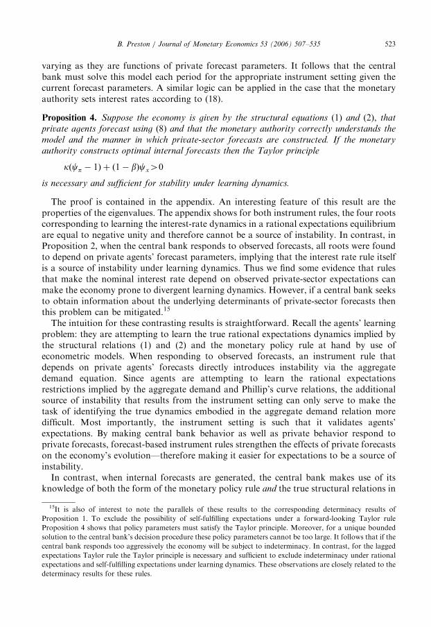
Fig. 1. A2 and A4 as a function of the policy parameter cp � 1.

B. Preston / Journal of Monetary Economics 53 (2006) 507–535 519

principle. The restriction A240 implies the following inequality:

cp þcx

k4

1

1� b�

2� b� abksð1� abÞ

.

Now consider taking the limit of the right hand side as b! 1. It is immediate that thesecond term converges to skð Þ�1, while the first goes to infinity. Hence the Taylor principlecannot be sufficient for E-Stability.

In order to make clear the practical relevance of this insight it is useful to pursue agraphical analysis. To this end, assume cx ¼ 0 so that the Taylor principle is given by therelation cp41, and make the following benchmark assumptions on remaining modelparameters: s ¼ 6:25; b ¼ 0:99; a ¼ 0:66 and k ¼ 0:024. The assumption on the policyparameter cx is made purely for convenience and matters little for the substantive pointsthat follow. The remaining parameter assumptions are taken from the estimates providedby Rotemberg and Woodford (1999).

Fig. 1 plots the values of A2 and A4 as a function of cp � 1� �

so that the positive orthantgraphs Ai;cp

� �pairs that are consistent with E-Stability (and satisfy the Taylor principle).

It is immediate that positive values for A2 and A4 require policy parameter coefficients inthe vicinity of 100—substantially above any empirically reasonable value.12 This suggestsnominal interest-rate rules that depend on private-sector expectations to be particularlyundesirable in terms of robustness. These basic insights show little sensitivity to alternativeparameter assumptions.13

These results contrast with the conclusions obtained by Bullard and Mitra (2002) whoconsider an economy given by (3) and (4) under the learning assumption to give a model ofthe monetary transmission mechanism of the form:

xt ¼ Etxtþ1 � s�1ðit � Etptþ1Þ þ rt, ð20Þ

pt ¼ bEtptþ1 þ kxt þ ut. ð21Þ

12The downward slopping curve is a parabola which eventually intersects the ordinate axes for large values of

the policy parameter.13For instance, with s ¼ 1 and all other parameters taking the same values, E-Stability requires cp450—still an

implausibly large value.


They find that the Taylor principle is necessary and sufficient for stability under the rules(17) and (18).14 As underscored by Preston (2005a), when the microfoundationsunderpinning this model are solved under the non-rational expectations assumption, thepredicted aggregate dynamics depend on long-horizon forecasts of inflation, output andthe nominal interest rate into the indefinite future. It is the presence of these additionalexpectational variables that present a non-trivial source of instability. By requiring agentsto forecast the future path of the nominal interest rate (that is, by requiring agents to learnthe rational expectations restrictions implied by the policy rule, which is not a property ofthe Bullard and Mitra model), in addition to the output gap and inflation rate, a moregeneral learning dynamic is admitted which in turn requires a stricter set of requirementson admissible policy parameters consistent with stability under learning. Indeed, numericalanalysis reveals that the three roots associated with the constant dynamics depend onprivate-sector beliefs.Thus, forecast-based instrument rules in an economy given by (1) and (2) are unlikely to

assist learnability of rational expectations equilibrium. Indeed, such rules may strengthenthe effects of private forecasts on the economy’s evolution by making central bankbehavior, as well as private behavior, respond to them. Such central bank behavior makesit easier for expectations to be a source of instability.To make clear that forecasting the future path of nominal interest rates is an important

source of instability, consider the following: suppose agents know the form of the policyrule (17). This means that agents know the restriction on nominal interest rates and one-period-ahead forecasts of inflation and the output gap that is required by the monetarypolicy rule to hold in a rational expectations equilibrium. Since agents understand thisrestriction to hold in all future periods we can substitute (17) for iT in (1) which combinedwith (2) gives the system

xt ¼ Et

X1T¼t

bT�t½ð1� b� scxÞxTþ1 þ sð1� cpÞpTþ1 � s{fT þ rT �, ð22Þ

pt ¼ kxt þ Et

X1T¼t

ðabÞT�t½kab � xTþ1 þ ð1� aÞb � pTþ1 þ uT �. ð23Þ

The crucial difference here, in contrast to (1) and (2), is that private agents need notindependently forecast the future path of the nominal interest rate—they need onlyforecast iT as a function of the forecasts of the future paths of inflation and the output gap.We therefore have a system of two equations in the unknowns ðpt;xtÞ. Under theassumption that agents know the policy rule (17) or (18) learning analysis yields thefollowing proposition.

Proposition 3. Suppose monetary policy is conducted according to either the rule (17) or (18)and the form of the particular rule is understood by agents to hold in all periods. The economy

is then given by the structural equations (1) and (2) and agents forecast the evolution of state

14Bullard and Mitra (2002) do not actually consider a Taylor rule that is capable of implementing the optimal

equilibrium. However, the rules proposed here differ only in terms of the exogenous disturbances that the bank is

responding to. As a result, the learning dynamics associated with agents’ estimated constants are equivalent to a

rule of the form considered by these authors since exogenous variables do not affect learning dynamics. See Evans

and Honkapohja (2003).


variables using (8). The Taylor principle

kðcp � 1Þ þ ð1� bÞcx40

is necessary and sufficient for E-Stability under least-squares learning dynamics.

The proof is contained in the appendix. Importantly, these stability results coincide withthe findings of Bullard and Mitra (2002) which considers forecast-based instrument rulesof the form of (17) or (18) in an economy described by relations (20) and (21). Thecontrasting findings of Propositions 2 and 3 stem from agents having to forecast the futurepath of nominal interest rates in the model presented in this paper. It follows immediatelythat requiring agents to learn the rational expectations restrictions embodied in the policyrule is an important source of instability; moreover, it underscores the source of differencein the stability conditions obtained here and those of Bullard and Mitra (2002) and directsattention to the potential importance of transparency in monetary policy design. Weconclude that the policy rules (17) and (18), by depending on observed private-sectorforecasts, can serve to make the equilibrium more susceptible to economic instability in thepresence of learning dynamics.

It is worth noting that transparency has been at the forefront of discussion on monetarypolicy design particularly in the recent inflation targeting literature. Indeed, Faust andSvensson (2001) present a model in which the central bank has an idiosyncracticemployment target which is imperfectly observed by the public. Fluctuations in this targetlead to central bank temptation to deviate from pre-announced inflation goals. However,increased transparency allows the private sector to observe the employment target withgreater precision and therefore raises the costs to the central bank of deviating from its pre-announced inflation objectives. Transparency is therefore desirable as it provides acommitment mechanism. Svensson (1999) further argues on the ground of this result thatfor inflation targeting central banks it is generally desirable for detailed information onpolicy objectives, including forecasts, to be published. Such transparency enhances thepublic’s understanding of the monetary policy process and raises the costs to a centralbank from deviating from its stated objectives. Proposition 3 shares this property: clearlyarticulating monetary policy strategy helps anchor private expectations and consequentlyassists in managing economic fluctuations.

More recently, and closely related to the present analysis, Orphanides and Williams(2005), and the introductory remarks on this paper by Bernanke and Woodford (2005) inthe same volume, highlight the advantages of publishing an inflation target. Orphanidesand Williams (2005) show in a simple model of the output-inflation trade off that if privateagents must learn about the inflation dynamics—in much the same way as in theframework of this paper—a more favorable trade off between inflation and output can beachieved if private agents are assumed to know the central bank’s long-run inflation targetrather than having to learn this quantity. Hence transparency of inflation objectives helpsanchor inflation expectations and facilitates stabilization of aggregate dynamics. Again,Proposition 3 is a result that is almost identical in spirit to this analysis. By publishing theadopted policy rule, private agents gain information that greatly assists determiningexpectations that are consistent with the equilibrium the central bank is seeking toimplement. Importantly, such transparency about the monetary policy process helps guardagainst the possibility that expectations are a source of instability.


6. Optimal internal forecasts

Suppose instead that the monetary authority constructs its own rational forecasts of thefuture path of the economy. The Taylor rules (17) and (18) are therefore interpreted asstipulating adjustment of the nominal interest rate in response to these internal forecasts.Does this give cause to alter our conclusion about the desirability of such monetarypolicies?To understand how such an internal forecast-based decision procedure for monetary

policy might be implemented, suppose that the monetary authority knows the true modelof the economy, and knows the way in which private agents construct forecasts. It followsthat the monetary authority can determine private-sector forecasts and solve for thetemporary equilibrium for inflation and output conditional on its current interest-ratesetting. These relations in conjunction with the instrument rule then provide a rationalexpectations model of the central bank’s interest rate setting procedure, which can besolved using standard methods. This solution determines the central bank’s currentinstrument choice and the values of output and inflation. These relations can then be usedto construct the E-Stability mapping from the private-sector’s forecast parameters to thecoefficients that would be rational given this evolution of the endogenous variables.More formally, take the case of the forward-looking Taylor rule. Substituting the private

forecasts (8) into the structural relations (1) and (2) implies the output gap and inflation tobe given by

pt ¼ ap þ bpLt�1 þ cput þ dprt þ epit, ð24Þ

xt ¼ ax þ bxLt�1 þ cxut þ dxrt þ exit, ð25Þ

where the coefficients ðai; bi; ci; d i; eiÞ for i 2 fp; xg are functions of the coefficientsðat; bt; ct; dtÞ of the current private-sector forecasting rule. These equations give the period t

inflation rate and output gap realizations, conditional on the current choice of the interestrate. Under the assumption that the monetary authority correctly understands the modelof the private sector, it can then construct forecasts of next period’s inflation and outputgap by leading (24) and (25) and taking expectations (rational) to give

Ecbt ptþ1 ¼ ap þ bpLt þ cpgut þ dprrt þ epE

cbt itþ1,

Ecbt xtþ1 ¼ ax þ bxLt þ cxgut þ dxrrt þ exE

cbt itþ1.

Substitution of these relations into the nominal interest-rate rule (17) yields an equation ofthe form

it ¼ ðcpap þ cxaxÞ þ ðcpbp þ cxbxÞLt þ ðcpcp þ cxcxÞgut

þ ðcpdp þ cxdxÞrrt þ ðcpep þ cxexÞEcbt itþ1

which is a linear rational expectations model of the central bank’s own behavior. If thecondition cpep þ cxex

�� o1 is satisfied, the model has a unique bounded solution, whichgives the interest-rate setting that the monetary authority chooses given its correctunderstanding of the model’s structural relations and the current parameters of privateagents’ forecasting rules. However, since we are describing a decision procedure of a singleactor in this economy, it is equally plausible to assume that the central bank solves thismodel concerning itself only with the minimum-state-variable solution regardless ofwhether jcpep þ cxexjo1 is true or not. Note also that the model’s coefficients are time


varying as they are functions of private forecast parameters. It follows that the centralbank must solve this model each period for the appropriate instrument setting given thecurrent forecast parameters. A similar logic can be applied in the case that the monetaryauthority sets interest rates according to (18).

Proposition 4. Suppose the economy is given by the structural equations (1) and (2), that

private agents forecast using (8) and that the monetary authority correctly understands the

model and the manner in which private-sector forecasts are constructed. If the monetary

authority constructs optimal internal forecasts then the Taylor principle

kðcp � 1Þ þ 1� bð Þcx40

is necessary and sufficient for stability under learning dynamics.

The proof is contained in the appendix. An interesting feature of this result are theproperties of the eigenvalues. The appendix shows for both instrument rules, the four rootscorresponding to learning the interest-rate dynamics in a rational expectations equilibriumare equal to negative unity and therefore cannot be a source of instability. In contrast, inProposition 2, when the central bank responds to observed forecasts, all roots were foundto depend on private agents’ forecast parameters, implying that the interest rate rule itselfis a source of instability under learning dynamics. Thus we find some evidence that rulesthat make the nominal interest rate depend on observed private-sector expectations canmake the economy prone to divergent learning dynamics. However, if a central bank seeksto obtain information about the underlying determinants of private-sector forecasts thenthis problem can be mitigated.15

The intuition for these contrasting results is straightforward. Recall the agents’ learningproblem: they are attempting to learn the true rational expectations dynamics implied bythe structural relations (1) and (2) and the monetary policy rule at hand by use ofeconometric models. When responding to observed forecasts, an instrument rule thatdepends on private agents’ forecasts directly introduces instability via the aggregatedemand equation. Since agents are attempting to learn the rational expectationsrestrictions implied by the aggregate demand and Phillip’s curve relations, the additionalsource of instability that results from the instrument setting can only serve to make thetask of identifying the true dynamics embodied in the aggregate demand relation moredifficult. Most importantly, the instrument setting is such that it validates agents’expectations. By making central bank behavior as well as private behavior respond toprivate forecasts, forecast-based instrument rules strengthen the effects of private forecastson the economy’s evolution—therefore making it easier for expectations to be a source ofinstability.

In contrast, when internal forecasts are generated, the central bank makes use of itsknowledge of both the form of the monetary policy rule and the true structural relations in

15It is also of interest to note the parallels of these results to the corresponding determinacy results of

Proposition 1. To exclude the possibility of self-fulfilling expectations under a forward-looking Taylor rule

Proposition 4 shows that policy parameters must satisfy the Taylor principle. Moreover, for a unique bounded

solution to the central bank’s decision procedure these policy parameters cannot be too large. It follows that if the

central bank responds too aggressively the economy will be subject to indeterminacy. In contrast, for the lagged

expectations Taylor rule the Taylor principle is necessary and sufficient to exclude indeterminacy under rational

expectations and self-fulfilling expectations under learning dynamics. These observations are closely related to the

determinacy results for these rules.


choosing its current instrument setting. Forecasts of output and inflation are formedoptimally, and, importantly, conditional on both its expected next-period choice of theinstrument and the current private forecast parameters. By taking explicit account ofthe effects of learning dynamics and its own future instrument choice on the evolutionof the economy, the monetary authority can offset any instability induced by a monetarypolicy rule that depends on private-sector forecasts. Thus the monetary authority, byconstructing forecasts optimally given private-sector behavior, chooses its instrument toaccommodate instability arising from private agents’ learning.

7. Alternative forecast-based instrument rules

The results presented thus far cast doubt on the usefulness of forecast-based instrumentrules for implementing optimal policy. Naive uses of observed private forecasts aresusceptible to divergent learning dynamics. While such instability problems can bemitigated—either by complete transparency with regards to the form of the monetarypolicy rule or detailed and accurate information on private agents’ long-horizonforecasts—it is natural to inquire as to whether there are other approaches toimplementing optimal monetary policy that are less informationally demanding.To this end, consider the following forecast-based instrument rule:

it ¼ clppt�1 þ cxEtxtþ1 þ cpEtptþ1 þ cuut þ crrt, (26)

where

cx ¼ cr ¼ 1=s; cu ¼ clp

and

clp ¼k� ls

ðk2 þ lþ blÞs; cp ¼

bkþ ðk2 þ lÞsðk2 þ lþ blÞs

.

Preston (2004) demonstrates this rule is consistent with implementing a timelessly optimalequilibrium that results when expectations are formed rationally and when the centralbank optimizes subject to a condition analogous to (10) written in terms if the price level.Note that this rule exhibits a different kind of history dependence relative to rules (17) and(18). Rather than responding to a lagged exogenous disturbance, it responds to the laggedprice level. Similarly, the response coefficients on observed forecasts are of a very differentkind than in the rules (17) and (18), only introducing one free policy parameter thatdetermines the central bank’s objective function. Nonetheless, this instrument rule isconsistent with implementing the timelessly optimal monetary policy.Preston (2004) shows that when the central bank observes private forecasts and

interprets the above rule as naively responding to such forecasts the adoption of (26)ensures stability under learning dynamics for a large range of plausible parametervalues (see Proposition 6 of that paper). For example, when a; b; y; g and r take thevalues 0.66, 0.99, 7.88, 0.35, 0.35, k 2 ð0; 1� and s 2 ð0; 2� E-stability always results.16

The rule (26) therefore provides an example of a class of rule that is less informationally

16Regions are considered for the parameters k and s as there is least agreement on their empirical value and the

results exhibit less sensitivity to the other parameter assumptions.


demanding than say the results of Proposition 4 but nonetheless achieves the central bank’sobjectives.

While a thorough examination of the performance of this rule relative to (17) and (18) isbeyond the scope of this paper, several points are worthy of note. First, such stabilityresults highlight that rules that depend on one-period-ahead forecasts need not necessarilylead to divergent learning dynamics. Second, it underscores that there are advantages tohaving instrument rules exhibit a particular kind of history dependence and a particularkind of dependence on available forecasts. Thus while the recent rational expectationsliterature promoting forecast-based instrument rules has typically eschewed rules withhistory dependence—presumably on the ground of simplicity—there may be good reasonsfor having such dependence: not only because optimal monetary policy is necessarilyhistory dependent in forward-looking rational expectations models but also because theymay have the desirable characteristic of promoting stability under non-rationalexpectations. Indeed, results of this kind are also found in Bullard and Mitra (2000)which shows that inertial Taylor rules—policies exhibiting dependencies on the previousperiod’s nominal interest rate—can help promote stability under learning. Third, andsomewhat more speculatively, it remains a challenge to identify whether rules exist thatinduce both determinacy of REE and stability under learning dynamics for all parametervalues and for central banks which only have limited information on the privateexpectations. The price-level targeting rules discussed in Preston (2004) and associatedimplied instrument rules such as (26) are promising in this regard.

8. Conclusions

This paper applies the framework of Preston (2005a) to understand the appropriate useof private forecasts in the design of monetary policy. The analysis demonstratesthat recently popular forecast-based instrument rules may give rise to divergent learningdynamics and therefore be undesirable as a means to stabilize economic fluctuations.In particular, the Taylor principle is not a sufficient condition for private agents tobe able to learn the associated rational expectations equilibrium. This result contrasts withrecent work by Bullard and Mitra (2002) which finds in an economy where only one-period-ahead expectations matter, that the Taylor principle is in fact necessary andsufficient conditions for stability under learning dynamics. Evidence on the importance ofa transparent monetary policy is also adduced by demonstrating that such instability canbe mitigated if private agents are informed about the form of the central bank’s instrumentrule. In this case, the Taylor principle is once more necessary and sufficient for stabilityunder learning.

However, if the central bank correctly understands the learning mechanism of privateagents, it can construct optimal forecasts conditional on private agents’ behavior. In thiscase, forecast-based instrument rules have the central bank respond to the determinants ofprivate forecasts, rather than the actual forecasts themselves, and this mitigates observedinstability problems of the former decision procedure. Indeed, the Taylor principle is againnecessary and sufficient for E-Stability. This underscores the importance of gatheringinformation on the nature and form of private forecasting methods. Moreover, itemphasizes that the concern of Bernanke and Woodford (1997), that policy rules whichnaively depend on observed private forecasts might be susceptible to problems ofindeterminacy, has greater ambit than rational expectations models.


Appendix A

This appendix first outlines the microfoundations of the model adopted in the main text.The general approach to analyzing learning dynamics in the context of this framework isthen discussed. It then turns to sketching the proofs of the central results which are allapplications of this general methodology. Since the algebra underpinning these results is attimes tedious, it is largely omitted. Most calculations were performed in Mathematica.

A.1. A simple model

A.1.1. Household and firm decision problems

The economy is populated by a continuum of households which seek to maximize futureexpected discounted utility

Ei

t

X1T¼t

bT�t UðCiT ; xT Þ �

Z 1

0

vðhiT ðjÞ; xT Þdj

� �, (27)

where utility depends on a consumption index, Cit, of the economy’s available goods (to be

specified), a vector of aggregate preference shocks, xt, and the amount of labor supplied forthe production of each good j, hi

ðjÞ. The second term in the brackets captures the totaldisutility of labor supply. The consumption index, Ci

t, is the Dixit-Stiglitz constant-elasticity-of-substitution aggregator of the economy’s available goods and has anassociated price index written, respectively, as

Cit �

Z 1

0

citðjÞðy�1Þ=y dj

� �y=ðy�1Þand Pt �

Z 1

0

ptðjÞ1�y dj

� �1=ð1�yÞ,

where y41 is the elasticity of substitution between any two goods and citðjÞ and ptðjÞ denote

household i’s consumption and the price of good j.17

Ei

t denotes the subjective beliefs of household i about the probability distribution of themodel’s state variables: that is, variables that are beyond agents’ control though relevant totheir decision problems—i.e. prices and exogenous variables. Beliefs are assumed to behomogenous across households, though each household has no knowledge of the beliefs ofother households. Agents therefore do not have a complete economic model of thedetermination of aggregate state variables and it is about the evolution of such variablesthat agents are attempting to learn. The learning algorithm is discussed below. Thediscount factor is assumed to satisfy 0obo1.Asset markets are assumed to be incomplete: there is a single one-period riskless non-

monetary asset available to transfer wealth intertemporally. Under this assumption, thehousehold’s flow budget constraint can be written as

Mit þ Bi

tp 1þ imt�1

� �Mi

t�1 þ ð1þ it�1ÞBit�1 þ PtY

it � Tt � PtC

it, (28)

where Mit denotes the household’s end-of-period holdings of money, Bi

t the household’send-of-period nominal holdings of risk-less bonds, im

t and it are the nominal interest ratespaid on money balances and bonds held at the end of period t, Y i

t the period income (real)

17The absence of real money balances from the period utility function (27) reflects the assumption that there are

no transaction frictions that can be mitigated by holding money balances. However, agents may nonetheless

choose to hold money if it provides comparable returns to other available financial assets.


of households and Tt denotes lump sum taxes and transfers. The household receivesincome in the form of wages paid, wðjÞ; for labor supplied in the production of each good,j. All households are assumed to own an equal part of each firm and therefore receive acommon share of profitsPtðjÞ from the sale of each firm’s good j. Period nominal income istherefore determined as PtY

it ¼

R 10½wtðjÞh

itðjÞ þPtðjÞ�dj for each household i. Fiscal policy

is assumed to be Ricardian. To summarize, the household’s problem in each period t is tochoose fci

tðjÞ; hitðjÞ;M

it;B

itg for all j 2 ½0; 1� so as to maximize (27) subject to the constraint

(28) taking as parametric the variables fpT ðjÞ;wT ðjÞ;PT ; iT�1; imT�1; xT g for TXt.

Firms face a Calvo-style price-setting problem in period t and maximize the expectedpresent discounted value of profits

Ei

t

X1T¼t

aT�tQt;T ½PiT ðptðiÞÞ�, (29)

where

PiT ðpÞ ¼ ytðiÞptðiÞ � wtðiÞhtðiÞ (30)

and ytðiÞ ¼ Y tðptðiÞ=PtÞ�y is the demand curve faced by producer i and output is produced

using technology ytðiÞ ¼ Atf ðhtðiÞÞ where At is an exogenous technology shock. Thefactor aT�t in the firm’s objective function is the probability that the firm will not beable to adjust its price for the next ðT � tÞ periods. Firms are assumed to value futurestreams of income at the marginal value of aggregate income in terms of the marginalvalue of an additional unit of aggregate income today. That is, a unit of income ineach state and date T is valued by the stochastic discount factor Qt;T ¼

bT�tPtUcðY T ; xT Þ=ðPT UcðY t; xtÞÞ. This simplifying assumption is appealing in the contextof the symmetric equilibrium that is examined in this model. To summarize, the firm’sproblem is to choose fptðiÞg to maximize (29) taking as given fY T ;PT ;wT ðjÞ;AT ;Qt;T g forTXt and j 2 ½0; 1�.

A.1.2. Optimal decision rules

Preston (2005a) shows that a log-linear approximation to the first order conditions ofthe above infinite horizon decision problems lead to following optimal decision rules. Eachhousehold allocates consumption according to

Ci

t � Y nt ¼ ð1� bÞ$i

t þ Ei

t

X1T¼t

bT�t½ð1� bÞxT � bsð{T � pTþ1Þ þ brT �,

where

Ci

t � lnðCit=Y Þ; Y t � lnðY t=Y Þ; {t � ln½ð1þ itÞ=ð1þ {Þ�, (31)

pt ¼ lnðPt=Pt�1Þ; $it ¼W i

t=ðPtY Þ

and for any variable g, g denotes the variables steady state value. The output gap xt ¼

Y t � Yn

t is the difference between output and the economy’s natural rate of output thatobtains in this model with fully flexible prices. It is a function of model disturbances as isthe natural rate of interest rt. Household wealth is defined as W i

tþ1 ¼ ð1þ imt ÞM

it þ ð1þ

itÞBit and s ¼ �Ucc=UcY40 is the intertemporal elasticity of substitution.


Each firm determines its optimal price according to

bp�t ðiÞ ¼ Ei

t

X1T¼t

ðabÞT�t 1� ab1þ oy

ðoþ s�1ÞxT þ abpT

� �,

where bp�t ðiÞ � lnðp�t ðiÞ=PtÞ and o40 is the elasticity of real marginal costs with respect toown output. Here the presence of long-horizon expectations arise due to the pricingfrictions induced by Calvo pricing. Integrating over the optimal decision rules of the abovehousehold and firm decision problems; applying the market clearing condition

R 10 C

i

t ¼ Y t;the definition of xt; noting that prices satisfy the relation pt ¼ bp�t ð1� aÞ=a; and droppingthe ‘^’ notation, gives the New Keynesian sticky-price model of output gap and inflationdetermination reported in the main text.

A.2. Expectational stability

Suppose monetary policy is conducted according to the rule

it ¼ cxxt�1 þ cuut þ crrt

where xt�1 is the lagged output gap. Standard analysis implies there exists a rationalexpectations equilibrium that is linear in the variables fxt�1; ut; rtg. If agents know the formof the minimum-state-variable solution they estimate a linear model

zt ¼ at þ bt � zt�1 þ ct � ut þ dt � rt þ �t, (32)

where zt ¼ ðpt;xt; itÞ0, �t is the usual error term, fat; bt; ct; dtg are coefficient parameter

vectors to be estimated. Relation (32) is called the agents’ perceived law of motion.Forecasts can then be constructed by solving this model forward and taking expectationsto give

EtzT ¼ ðI3 � btÞðI3 � bT�tt Þat þ bT�t

t zt þ gutðgI3 � btÞ�1ðgT�tI3 � bT�t

t Þct


t Þdt ð33Þ

for TXt. To obtain the actual law of motion, substitute (33) into the system of equations(1) and (2). Collecting like terms gives a general expression of the form

zt ¼ at þ btxt�1 þ ctut þ d trt,

where fat; bt; ct; d tg are functions of the current private forecast parameters fat; bt; ct; dtg.Leading this expression one period and taking expectations (rational) provides

Etztþ1 ¼ at þ btxt þ ctgut þ d trrt

which describes the optimal rational forecast conditional on private-sector behavior.Taken together with (33) at T ¼ tþ 1 it defines a mapping that determines the optimalforecast coefficients given the current private-sector forecast parameters ða0t; b

0tÞ, written as

Tðat; bt; ct; dtÞ ¼ ðat; bt; ct; d tÞ. (34)

A rational expectations equilibrium (REE) is a fixed point of this mapping. For suchREE, we are interested in asking under what conditions does an economy with learningdynamics converge to this equilibrium. Using stochastic approximation methods,Evans and Honkapohja show that the conditions for convergence of the learning (6)and (7) are neatly characterized by the local stability properties of the associated ordinary


differential equation

d

dtða; b; c; dÞ ¼ Tða; b; c; dÞ � ða; b; c; dÞ, (35)

where t denotes ‘‘notional’’ time. The REE is said to be expectationally stable, or E-Stable,if this differential equation is locally stable in the neighborhood of the REE. Fromstandard results for ordinary differential equations, a fixed point is locally asymptoticallystable if all eigenvalues of the Jacobian matrix D½Tða; b; c; dÞ � ða; b; c; dÞ� have negativereal parts (where D denotes the differentiation operator and the Jacobian is understood tobe evaluated at the rational expectations equilibrium of interest.) See Evans andHonkapohja (2001) for further details on expectational stability.

Appendix B. Proof of Proposition 2

Consider the case of the forward-looking Taylor rule. We assume that private agents aneconometric model that is linear in fLt�1; ut; rtg. Forecasts are therefore constructedaccording to the relation


t Þ�1at þ bT�t

t zt þ gutðgI4 � btÞ�1ðgT�tI4 � bT�t

t Þct


t Þdt ð36Þ

for T4t; where zT ¼ ðpT ; xT ; iT ;LT Þ, and ðat; bt; ct; dtÞ are the estimated coefficientmatrices defined in Section 2.3. Substituting the forecasts into the structural relations givesthe temporary equilibrium from which the E-Stability mapping can be constructed. Theconditions for E-Stability are then given by the local stability properties of the Jacobian ofthe associated ordinary differential equation

T 0ðfÞ � I16 ¼

A1 � I4 A5 0 0

0 A2 � I4 0 0

0 A6 A3 � I4 0

0 A7 0 A4 � I4

26664

37775,

where f ¼ ða0t; bp;t; bx;t; bi;t; bL;t; c0t; d0tÞ0, I4 and I16 identity matrices of stated dimension and

the Ai matrices have dimension ð4� 4Þ and elements that are composites of modelparameters. E-Stability requires all roots of this system to have negative real parts. Theroots are clearly determined by the properties of the matrices A1 � I4;A2 � I4; A3 � I4 andA4 � I4. A1 can be shown to be given by

A1 ¼

ð1�aÞb1�ab þ k s

1�b� scp

� �abk1�abþ kð1� scxÞ �

ksb1�b a14

s1�b� scp 1� scx �

sb1�b a24

cp cx 0 a34

0 0 0 0

2666664

3777775,

where a14; a24 and a34 are composites of model primitives. It follows that A1 � I4 has oneroot equal to negative unity and the remaining roots determined by the characteristicequation

PðlÞ ¼ l3 þ A2l2þ A1lþ A0


and stability under learning dynamics requires A0; A240 and A4 ¼ �A0 þ A1A240, whereAi are composites of model primitives. The first two conditions can be shown to imply therestrictions

cp þ1� bk

cx41

and

cp þcx

k4

ksð1� abÞ � ð1� bÞ2 � ð1� bÞð1� abÞksð1� bÞð1� abÞ

.

The former clearly established the Taylor principle to be necessary for E-Stability.However, it is not sufficient for all parameter values under the maintained assumptions. Tosee this consider the RHS constant term of the second restriction. It can be written as

1

1� b�

2� b� abksð1� abÞ

.

As b! 1 this expression tends to infinity so that the Taylor principle is necessarilyviolated for a given policy setting ðcp;cxÞ. Since the graphical analysis suggest that forreasonable parameter values E-Stability is unlikely to obtain given these conditions alone,the analysis of the conditions from A2 � I4; A3 � I4 and A4 � I4 that relate to learning theslope coefficients on each state variable are not developed. In the author’s experience, theconstant coefficients typically imply the strictest conditions.Now consider the case of the lagged-expectations Taylor rule. The economy is given by

the system of equations (1), (2) and the monetary policy rule (18). In contrast to theforward-looking Taylor rule, rational expectations equilibrium is linear in the variablesfLt�1; ut�1; rt�1g. Thus agents use an econometric model of the form

zt ¼ at þ btzt�1 þ ctut�1 þ dtrt�1 þ et

zT ¼ ðpT ; xT ; iT ;LT Þ to construct forecasts as


t Þat þ bT�tt zt þ utðgI4 � btÞ

�1ðgT�tI4 � bT�t

t Þct

þ rtðrI4 � btÞ�1ðrT�tI4 � bT�t

t Þdt. ð37Þ

It is immediate that the forecasts of the constant dynamics are identical to the forward-looking Taylor rule. It follows that the results derived for that case apply here, so that theTaylor principle is again necessary but not sufficient.

Appendix C. Proof of Proposition 3

Consider the case of the forward-looking Taylor rule. We assume that private agents aneconometric model that is linear in fLt�1; ut; rtg. Forecasts are therefore constructedaccording to the relation (36) for T4t; where zT ¼ ðpT ;xT ;LT Þ is redefined recallingprivate agents no longer need to forecast the future path of interest rates, and ðat; bt; ct; dtÞ

are the estimated coefficient matrices defined in Section 2. Substituting the forecasts intothe structural relations gives the temporary equilibrium from which the E-Stabilitymapping can be constructed. The conditions for E-Stability are then given by the local


stability properties of the Jacobian of the associated ordinary differential equation

T 0ðfÞ � I12 ¼

A1 � I3 A5 0 0

0 A2 � I3 0 0

0 A6 A3 � I3 0

0 A7 0 A3 � I3

26664

37775,

where f ¼ ða0t; bp;t; bx;t; bL;t; c0t; d0tÞ0 when evaluated at the rational expectations equilibrium

of interest, I3 and I12 identity matrices of stated dimension and the Ai matrices havedimension ð3� 3Þ and elements that are composites of model parameters and 0 is a nullmatrix of similar dimension. E-Stability requires all roots of this system to have negativereal parts. The roots are clearly determined by the properties of the matrices A1 � I4;A2 �

I4;A3 � I4 and A4 � I4: All Ai � I3 have characteristic equations of the form

PðlÞ ¼ ð1þ lÞðl2 þ A1lþ A0Þ

therefore having one eigenvalue equal to negative unity. The remain two roots will benegative if and only if A0; A240: In the case of A1 � I3 these latter two inequalities can beshown to imply the restrictions

cp þ1� bk

cx41

and

cp þcx

k41�

ð1� bÞ2

ð1� abÞks.

The former clearly established the Taylor principle to be necessary for E-Stability. Similararguments to those employed in the proof of Proposition 2 establish satisfaction of theTaylor principle as being sufficient the latter to hold.

Similarly, A2 � I3 has the remaining two roots being negative if and only if therestrictions

cp þð1� bmÞ

kcx41�

ð1� mÞð1� mbÞks

and

cp þcx

k41�

ð1� bmÞ2 þ ð1� mÞð1� abmÞð1� abmÞksm

which are again satisfied if the Taylor principle is satisfied (using the same arguments asProposition 2) and noting 0omo1. The proof is complete by observing that A3 � I3 andA4 � I3 take an identical form to A2 � I3 once m is replaced by r and g, respectively. Since0or; go1 the result follows immediately.

In the case of the lagged expectations Taylor rule, almost identical calculations give theresult that the Taylor principle is necessary and sufficient for E-Stability.

Appendix D. Proof of Proposition 2

Consider the case of the forward-looking Taylor rule. Section 6 showed that themonetary authority’s decision problem each period is to solve the rational expectations


problem

it ¼ ðcpap þ cxaxÞ þ ðcpbp þ cxbxÞLt þ ðcpcp þ cxcxÞgut

þ ðcpdp þ cxdxÞrrt þ ðcpep þ cxexÞEcbt itþ1

¼ ai þ biLt�1 þ ciut þ d irt þ eiEcbt itþ1,

where

ai ¼ ðcpap þ cxaxÞ; bi ¼ ðcpbp þ cxbxÞm,

d i ¼ ðcpdp þ cxdxÞr; ei ¼ ðcpep þ cxexÞ,

ci ¼ ðcpcp þ cxcxÞgþ ðcpbp þ cxbxÞ.

If jeijo1 there is a unique bounded solution. Solving forward gives

it ¼ Et

X1s¼0

esi ½ai þ biLtþs�1 þ ciutþs þ d irtþs�. (38)

Noting

EtLtþs ¼ msX1j¼0

mjut�j þ Et

Xs�1j¼0

mjutþs�j

¼ msLt þgðgs � msÞ

g� mut

and evaluating expectations in (38) gives

it ¼ai

1� ei

þbi

1� eimLt�1 þ

biei þ cið1� eimÞð1� eimÞð1� eigÞ

ut þd i

1� eirrt

as the required solution. This, together with

pt ¼ ap þ bpLt�1 þ cput þ dprt þ epit, ð39Þ

xt ¼ ax þ bxLt�1 þ cxut þ dxrt þ exit ð40Þ

solves for the temporary equilibrium values of fpt;xt; it;Ltg. Leading these equations oneperiod and taking expectations gives the optimal forecasts given this evolution of theendogenous variables.The Jacobian matrix of the associated ordinary differential equation can be shown to be

given by

T 0ðfÞ � I16 ¼

A1 � I4 A5 0 0

0 A2 � I4 0 0

0 A6 A3 � I4 0

0 A7 0 A4 � I4

26664

37775,

where f0 ¼ ða0t; bp;t; bx;t; bi;t; bL;t; c0t; d0tÞ, I4 and I16 are identity matrices of the indicated

dimension, 0 a 4� 4ð Þ null matrix and the Ai matrices have elements that are composites ofmodel primitives.For E-Stability A1 � I4, A2 � I4, A3 � I4 and A4 � I4 must each have four roots with

negative real parts. Consider A1 � I4. It is easily shown that two roots are equal to


negative unity, while the remaining two roots are the solution to the quadratic equation

al2 þ blþ c ¼ 0,

where

a ¼ ð1� bÞð1� abÞð1þ sðcx þ kcpÞÞ,

b ¼ G0 þ G1c1 þ G2cp,

c ¼ skðcp � 1Þ þ sð1� bÞcx

and

G0 ¼ ð1� bÞ2 � ksð1� abÞ,

G1 ¼ s½ð1� bÞ2 þ ð1� abÞ�,

G2 ¼ ks½ð1� bÞ þ ð1� abÞ�.

Under the maintained model assumptions a40. For a two roots with negative real partswe require b; c40. The latter restriction requires

cp þ cx �1� bk

41

establishing the Taylor principle to be necessary for E-Stability. b40 implies

cp þ cx �½ð1� bÞ2 þ ð1� abÞ�k½ð1� bÞ þ ð1� abÞ�

4ksð1� abÞ � ð1� bÞ2

ks½ð1� bÞ þ ð1� abÞ�.

Since the right-hand side constant is clearly less than unity and the coefficient on the policyparameter cx greater than ð1� bÞ=k we infer that the Taylor principle is also sufficient forsatisfaction of this restriction.

For A2 � I4 identical manipulations show that two roots are equal to negative unity,while the remaining two roots are the solution to the quadratic equation

al2 þ blþ c ¼ 0,

where

a ¼ ð1� bmÞð1� abmÞð1þ mscx þ mkscpÞ,

b ¼ G0 þ G1cx þ G2cp,

c ¼ ksðcp � 1Þ þ smð1� bmÞcx þ ð1� bmÞð1� mÞ

and

G0 ¼ ð1� bmÞ2 þ ð1� mÞð1� abmÞ � ksmð1� abmÞ,

G1 ¼ sm½ð1� bmÞ2 þ ð1� abmÞ�,

G2 ¼ ksm½ð1� bmÞ þ ð1� abmÞ�.

Again under the maintained model assumptions a40. For the final two roots to havenegative real parts we require b; c40 implying the restrictions

cp þ cx �½ð1� bmÞ2 þ ð1� abmÞ�k½ð1� bmÞ þ ð1� abmÞ�

4ksmð1� abmÞ � ½ð1� bmÞ2 þ ð1� mÞð1� abmÞ�

ksm½ð1� bmÞ þ ð1� abmÞ�


and

cp þ cx �ð1� bmÞ

k4

ksm� ð1� mÞð1� abmÞksm

.

It is again easy to show that under the maintained model assumptions both theseinequalities have right-hand side constants that are less than unity and slope coefficients onthe parameter cx that are greater than ð1� bÞ=k which establishes the Taylor principle asbeing necessary and sufficient for E-Stability conditions on A2 � I4 to be satisfied. Similarcalculations demonstrate the matrices A3 � I4 and A4 � I4 to imply the same conditions asA2 � I4. Therefore the Taylor principle is necessary and sufficient for E-Stability.For the lagged expectations Taylor rule the proof is virtually identical to the case of the

forward-looking Taylor rule. It is omitted here, and available from the author on request.

References

Batini, N., Haldane, A.G., 1999. Forward-looking rules for monetary policy. In: Taylor, J. (Ed.), Monetary Policy

Rules. University of Chicago Press, Chicago.

Bernanke, B.S., Woodford, M., 1997. Inflation forecasts and monetary policy. Journal of Money, Credit, and

Banking 29 (4), 653–686.

Bernanke, B.S., Woodford M., 2005. Introduction. In: Bernanke B.S., Woodford, W., (Eds.), The Inflation

Targeting Debate. University of Chicago Press.

Bullard, J., Mitra, K., 2000. Determinacy, learnability and monetary policy inertia. Working Paper No. 2000-

030A, Federal Reserve Bank of St. Louis. [Available online at http://www.stls.frb.org/docs/research/wp/2000-

001.pdf].

Bullard, J., Mitra, K., 2002. Learning about monetary policy rules. Journal of Monetary Economics 49 (6),

1105–1129.

Clarida, R., Gali, J., Gertler, M., 1998. Monetary policy rules in practice: some international evidence. European

Economic Review 42, 1033–1067.

Clarida, R., Gali, J., Gertler, M., 1999. The science of monetary policy: a New Keynesian perspective. Journal of

Economic Literature 37, 1661–1707.

Clarida, R., Gali, J., Gertler, M., 2000. Monetary policy rules and macroeconomic stability: evidence and some

theory. Quarterly Journal of Economics 115, 147–180.

Evans, G.W., Honkapohja, S., 2001. Learning and Expectations in Economics. Princeton University Press,

Princeton, NJ.

Evans, G.W., Honkapohja, S., 2002. Monetary policy, expectations and commitment. Working Paper.

Evans, G.W., Honkapohja, S., 2003. Expectations and the stability problem for optimal monetary policies.

Review of Economic Studies 70 (4).

Faust, J., Svensson, L., 2001. Transparency and credibility: monetary policy with unobservable goals.

International Economic Review 42, 369–397.

Giannoni, M.P., Woodford, M., 2002a. Optimal interest-rate rules: I. General theory. Unpublished, Columbia

University.

Giannoni, M.P., Woodford, M., 2002b. Optimal interest-rate rules: II. Applications. Unpublished, Columbia

University.

Hall, R.E., Mankiw, N.G., 1994. Nominal income targeting. In: Mankiw, N.G. (Ed.), Monetary Policy, p. 71.

Honkapohja, S., Mitra, K., 2004. Are non-fundamental equilibria learnable in models of monetary policy?

Journal of Monetary Economics 51, 1743–1770.

Honkapohja, S., Mitra, K., 2005. Performance of monetary policy with internal central bank forecasting. Journal

of Economic Dynamics and Control 29 (4), 627–658.

Levin, A., Wieland, V., Williams, J.C., 2003. Robustness of forecast-based monetary policy rules under model

uncertainty. American Economic Review 93, 622–645.

McCallum, B.T., 1983. On non-uniqueness in rational expectations models: an attempt at perspective. Journal of

Monetary Economics 11, 139–168.

http://www.stls.frb.org/docs/research/wp/2000-001.pdf

http://www.stls.frb.org/docs/research/wp/2000-001.pdf


McCallum, B.T., 1999. Issues in the design of monetary policy rules. In: Taylor, J., Woodford, M. (Eds.),

Handbook of Macroeconomics. North-Holland, Amsterdam.

Orphanides, A., Williams, J.C. 2005 Imperfect knowledge, inflation expectations, and monetary policy. In:

Bernanke, B.S., Woodford, M., The Inflation Targeting Debate. University of Chicago Press.

Preston, B., 2004. Adaptive learning and the use of forecasts in monetary policy. Unpublished, Columbia

University.

Preston, B., 2005a. Learning about monetary policy rules when long-horizon expectations matter. International

Journal of Central Banking 1 (2), 81–126.

Preston, B., 2005b. Adaptive learning in infinite horizon decision problems. Unpublished, Columbia University.

Rotemberg, J., Woodford, M., 1999. Interest-rate rules and an estimated sticky-price model. In: Taylor, J. (Ed.),

Monetary Policy Rules. University of Chicago Press, Chicago.

Svensson, L.E., 1999. Inflation targeting as a monetary policy rule. Journal of Monetary Economics 43, 607–654.

Svensson, L.E., Woodford, M., 2002. Implementing optimal monetary policy through inflation forecast targeting.

Unpublished manuscript, Princeton University.

Woodford, M., 1999. Optimal monetary policy inertia. NBER Working Paper 7261.

Woodford, M., 2003. Interest and Prices: Foundations of a Theory of Monetary Policy. Princeton University

Press, Princeton, NJ.

Date post:	05-Sep-2016
Category:	Documents
Upload:	bruce-preston
View:	213 times
Download:	0 times

Adaptive learning, forecast-based instrument rules and monetary policy

Documents