Accepted Manuscript

Adaptive Localized Replay: An efficient integration scheme foraccurate simulation of coarsening dynamical systems

Scott A. Norris, Skyler Tweedie

PII: S0021-9991(14)00335-0DOI: 10.1016/j.jcp.2014.05.003Reference: YJCPH 5249

To appear in: Journal of Computational Physics

Received date: 17 October 2013Revised date: 1 May 2014Accepted date: 2 May 2014

Please cite this article in press as: S.A. Norris, S. Tweedie, Adaptive Localized Replay: Anefficient integration scheme for accurate simulation of coarsening dynamical systems, Journalof Computational Physics (2014), http://dx.doi.org/10.1016/j.jcp.2014.05.003

This is a PDF file of an unedited manuscript that has been accepted for publication. As aservice to our customers we are providing this early version of the manuscript. The manuscriptwill undergo copyediting, typesetting, and review of the resulting proof before it is publishedin its final form. Please note that during the production process errors may be discovered whichcould affect the content, and all legal disclaimers that apply to the journal pertain.

Adaptive Localized Replay: an efficient integration scheme for

accurate simulation of coarsening dynamical systems

Scott A. Norris and Skyler Tweedie

May 8, 2014

Department of Mathematics

Southern Methodist University

Abstract

Coarsening dynamical systems (CDS) of ordinary differential equations (ODEs) have as a defining feature the

presence of discontinuities in the governing equations, due to the removal of vanishing elements from the system.

Simple, commonly-used integration strategies for ODEs neglect these discontinuities, resulting in large errors. In

contrast, available methods to resolve discontinuities exhibit total running times that scale like O(N2

)as the number

of elements N → ∞. The resulting need to choose between either speed or accuracy frustrates attempts to gather

well-converged statistical data from large ensembles of elements, a common goal in studies of coarsening.

In this work, we introduce a numerical scheme, called Adaptive Localized Replay (ALR), which overcomes

this dilemma, provided the underlying system has sparse neighbor dependence. By analyzing the system after each

timestep, and then selectively re-simulating only those (small) parts of the system that were affected by discontinu-

ities, we attain high-order accuracy while maintaining running times of O (N). Using a reference implementation of

our algorithm, applied to a sample problem from the field of faceted surface evolution, we obtain convergence and

runtime results for the ALR method, which compares favorably with existing methods.

1 Introduction

The characterization of micro-structured materials is a fundamental issue in materials science, since the statistics

of microstructural morphology play a central role in determining effective material properties. In many regimes of

growth or relaxation, microstructured materials can exhibit coarsening, during which small microstructural features

continually decrease in size until they vanish, causing the average lengthscale of those that remain to increase with

time. Of particular interest, many such systems exhibit dynamic scaling, whereby the microstructural variations ap-

proach a constant statistical state even as the length scale increases. This behavior is of intense interest, because if the

scale-invariant state can be understood theoretically, and its dependence on environmental parameters predicted, then

one has the possibility for creating predictable and controllable microstructures at a statistical level, despite a lack of

control over the structural evolution at any single location within the material.

A particularly interesting coarsening system for the study of scaling phenomena is that of completely faceted

surfaces. These have an inherent structural simplicity that arises because each facet in such a system moves as a single

unit. Hence, in many cases, the nonlinear PDEs that fully describe the system (e.g., [1, 2, 3, 4]) can be simplified

1

via asymptotic analysis to a facet velocity law providing the normal velocity of each facet (e.g., [5, 6, 7, 8, 9, 10]).

Because the facet velocity law specifies the interfacial velocity of a continuous surface by means of discrete, constant

quantities, the computational complexity of simulating the surface evolution reduces to that of a system of ordinary

differential equations (ODEs). In essence, the surface is governed by a dynamical system of the form

dxdt

= f(x) , (1)

with the vector x containing one entry per facet, but where the dimension of the system decreases every time a coars-

ening event happens. The resulting structure has been termed a Coarsening Dynamical System (CDS), and the relative

simplicity of the governing equations, combined with the easy availability of standard numerical solvers, represent

notable attractions of the faceted surface problem relative to other coarsening problems. Accordingly, this approach

has been employed frequently for one-dimensional surfaces [11, 12, 13, 8, 10, 14, 15, 16, 17, 18], although less so for

two-dimensional simulation [19, 20, 21, 22, 23, 9, 24], where the resolution of topological events becomes the dom-

inant computational cost (note that the use of phase-field [25, 26] or level-set [21, 22, 27] methods avoid the manual

resolution of topological events, at the cost of losing the structure exhibited by Eq.(1)).

For the detailed study of scale-invariance exhibited by coarsening faceted surfaces, it is necessary to gather statis-

tics on the average geometric properties of the system (e.g., the coarsening exponent [28, 29]), to use as the basis for,

or test of, theories attempting to explain or predict the statistical behavior [23, 30]. In order to get well-converged

statistics, one typically wants to simulate systems with as many elements as possible. This is facilitated by the simple

structure of Eq.(1); however, coarsening systems can easily lose most of their elements prior to reaching the scale-

invariant state, and so reasonable convergence within that state can require truly enormous numbers of initial elements.

In order to perform such large simulations as quickly as possible, large timesteps are naturally desired. Finally, to en-

sure that these large timesteps do not introduce too much error into the gathered statistics, one ideally would like to

use high-order methods. Hence, for the acquisition of statistics from the simulation of very large CDSs, the use of

high-order methods for numerical ODEs is highly desired.

It turns out, however, that the use of standard high-order methods on CDS problems with the form (1) is prob-

lematic. Faceted surfaces, in particular, often exhibit facet velocity laws that are configurational, depending on local

facet geometry. During the coarsening process, topological changes to the surface can alter these geometries suddenly,

which means that the resulting dynamical system is generically discontinuous in time. Besides the theoretical prob-

lems posed by these discontinuities, there are computational problems as well. Specifically, the times of the coarsening

events are not known in advance, and generic ODE solvers inevitably overstep these times. Sudden, discontinuous

changes to a few components of the system, if not detected properly, induce errors proportional to the timestep length.

Although algorithms for avoiding these errors exist, the standard method of doing so involves reverting the entire

system to the time a discontinuity occurred, updating the system, and then proceeding. Because the discontinuities are

typically localized during a given timestep, reverting the whole system is extremely wasteful, consuming most of the

computational time in the simulation. Because both the speed and accuracy of simulations are currently limited in this

way, the quantity and quality of statistics that can be gathered and used to test theories is also limited.

In this manuscript we introduce a method for the simulation of Eq.(1) that avoids the poor scaling of traditional

methods for handling discontinuities, while preserving their accuracy, by exploiting the nearest-neighbor structure

of most facet evolution laws. We begin by quantifying the error induced by ignoring the discontinuity altogether

during a timestep of length Δt, and show that for systems with nearest-neighbor dependency structures, the error

scales like ΔtD, where D is the neighbor distance away from the facet exhibiting the discontinuity. Hence, if one

wishes to preserve an O(ΔtP

)method, one only needs to correct the outcome of the directly affected facets, and the P

2

nearest neighbors to each side. This can be done by carefully re-simulating only small subdomains of facets associated

with each coarsening event, and using polynomial interpolations of further neighbors to close the system at a small

size. To ensure the accurate correction of such subdomains, an adaptive approach is required that gracefully fails if

unanticipated events are detected, lending the algorithm the name of Adaptive Localized Replay.

2 An example problem and a reference method.

Specific examples of the kinds of CDSs described in the introduction include asymptotic reductions of the 1D Cahn-

Hilliard equation for spinodal decomposition [31], and the generalized convective Cahn-Hilliard equation [13, 2, 8]:

ut +αuux =

{δδu

[F (u)+

12(ux)

2]}

xx=[F ′ (u)− εuxx

]xx . (2)

Here u(x, t) is an order parameter describing the phase of the system, F (u) is a double-welled energy potential driving

the system toward one well or the other, ε is a small parameter penalizing rapid changes in u(x, t), and α measures

the strength of a non-conserved driving force. The variational structure of the right-hand side drives the system into

a configuration consisting of large alternating domains where u is nearly equal to one of the two minimizers of F (u),

separated by rapid transitions between the two values, called “steps” or “kinks”.

Asymptotic analysis of Eq.(2) leads to relatively simpler expressions for the evolution of the step locations, and

hence, of the domain sizes, which we will denote {xi}. For the original Cahn-Hilliard equation (α = 0), encountered

in studies of phase separation, the CDS governing domain size evolution take the form [32, 33, 34]

dxi

dt=

1xi+1

[exp(−xi+2)− exp(−xi)]+1

xi−1[exp(−xi)− exp(−xi−2)] . (3)

More recently, the convective form of the Cahn-Hilliard equation (α > 0) has received much attention, appearing in

particular during the solidification of an anisotropic material into an undercooled melt [2]. An asymptotic analysis of

the CCH shows that the resulting CDS for the domain sizes is [13, 8]

dxi

dt= (−1)i

[1

exp(xi+1)−1− 1

exp(xi−1)−1

]. (4)

To most clearly communicate the essential features of our algorithm, we will here consider a simpler CDS, en-

countered in the directional solidification of binary alloys [35, 10]. Under a simple negative effective thermal gradient,

the vertical velocity of each facet is simply proportional to the vertical co-ordinate of its midpoint, leading to a CDS

on the facet widths ofdxi

dt=

14[2xi − xi−1 − xi+1] . (5)

We are not concerned with the specifics of this system, but for the illustration of a numerical algorithm, it has ad-

vantages over Eqs.(3)-(4). In contrast to Eq.(3), it has a simpler structure, with the rate of change of each domain

length depending only on the nearest neighbors. And, in contrast to Eq.(4), it is continuous for all values of the {xi}.

Nevertheless, it shares important general properties with Eqs.(3)-(4). In particular, we can immediately see that this

system will lead to coarsening. If any particular facet xi is much shorter than the average facet length, then on average,

the right-hand side of Eq.(5) is negative, and the length will continue decreasing until it reaches zero. Assuming that

facet slopes alternate, a zero-length facet causes its own elimination, and also the merger of its two neighbors into a

3

position x

time

t

(a)

position x

t3

t2

t1

heig

ht h

hillvalley

(b)

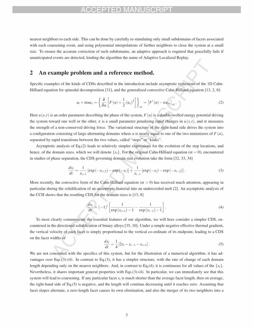
Figure 1: (color online) (a) A schematic of a coarsening event. The small facet shrinks in size until it vanishes,causing the annihilation of the bounding convex/concave corners, and the merger of its two neighbors into a single,larger facet. (b) A visualization of part of the simulation of a large surface, showing the location of corners colored asin (a); coarsening events occur whenever two corners meet and annihilate.

single, larger facet with length equal to the sum of the neighbors [35]:

(· · · ,xi−1,xi,xi+1, · · ·) xi→0+−−−−→ (· · · ,xi−1 + xi+1, · · ·). (6)

A single coarsening event of this nature is illustrated in Figure 1a, and a representative simulation of Eq.(5) containing

many such events is illustrated in Figure 1b.

By this point, it is clear that the system of equations (5), and any equation with similar behavior, is inherently

discontinuous - for every coarsening event (6), the right-hand side of the equation x = f (x) changes qualitatively, not

just in its values but also in its dimensionality. And the coarsening events that cause these discontinuities can happen

at any time, statistically always in between timesteps. Hence, it is necessary to consider the numerical simulation of

ODEs with discontinuities. We shall conclude this section by outlining some existing methods for numerical simula-

tion of discontinuous ODEs, and highlighting important limitations that render them unsuitable for the simulation of

large facet ensembles necessary for statistics.

2.1 Fast but Inaccurate: Ignoring the discontinuity.

The easiest way to simulate Eq.(5), used by many authors studying coarsening phenomena (see, e.g. Refs. [13, 8]),

is simply to use a standard solver to iterate Eqs.(5), and perform coarsening events only at the discrete times visited

by the solver. This is typically accomplished by removing, prior to each step, all facets below some small threshhold

4

value (an “early” fix); one could also remove, after each step, all facets whose length has become negative (a “late”

fix). A simple algorithm describing this approach is the following:

Algorithm 1

Step 1. Take a timestep from tn to tn+1 using a standard ODE solver.

Step 2. List all facets whose values crossed threshhold (or became negative) during the timestep.

Step 3. Eliminate those facets from the system, and patch the surface in a physically-consistent way.

where “physically-consistent” means preserving the total length of both positive and negative-sloped facets. This ap-

proach, although rather simplistic, is rather easy to implement, with only the repair in Step 3 requiring some geometric

considerations. It is also quite efficient, allowing rapid exploration of large ensembles of facets.

Unfortunately, although it is fast and easy to program, Algorithm 1 is also fundamentally limited to being first-

order accurate in time, with errors proportional to the timestep taken. For, suppose facet i vanished during timestep j

at a time t∗ ∈ (t j, t j+1

). Then the true governing equations were

dxdt

=

⎧⎨⎩

f1 (x) t ∈ (t j, t∗)

f2 (x) t ∈ (t∗, t j+1

) , (7)

whereas Algorithm 1 simply uses one of these equations for the entire timestep (the second equation if performing

“early” fixes, and the second if performing “late” fixes). At coarsening events, the right hand side of Eqs.(5) can

change by an amount proportional to the average facet length – i.e., by an O (1) amount. By neglecting the change

in the equations that should have occurred at t = t∗, Algorithm 1 therefore used equations wrong by O (1) for a time

duration proportional to Δt, leading to an error of size O (Δt). Hence, Algorithm 1 can never be more than first-order

accurate, regardless of the underlying solver used to integrate the equations (indeed, results on the accuracy of standard

solvers are built upon the assumption of sufficiently smooth solutions). Any significant degree of accuracy would thus

require very small timesteps, rendering this method unsuitable for the rapid simulation of very large systems.

2.2 Accurate but slow: Full Replay of each discontinuity

A much more accurate method, which does not often appear in the coarsening literature but is still relatively simple

to code, is to estimate the time of a discontinuity using an interpolating polynomial associated with the numerical

solution [36]. One can then revert the system to this time, update the right-hand side of Eqs.(5) to the correct state, and

continue the integration onward [37]. Specifically, given the state of the system xn at time tn, we find the state xn+1 at

time tn+1 using the following algorithm:

Algorithm 2

Step 1. Take a full timestep to t = tn+1 with an ordinary ODE solver.

Step 2. Find the time t∗ of the earliest vanishing facet, using a root-finder on interpolating polynomials.

Step 3. Move the entire system back to time t∗ (using either the solver itself, or the interpolating polynomial).

Step 4. Update the state of the data structure and equations to reflect the appropriate coarsening event.

Step 5. Take the rest of the step, from t∗ to tn+1. If additional events are found, return to Step 2.

5

We shall call this method the Full Replay method, in that once a discontinuity is detected, the full system is reverted

to the discontinuity time, and then re-simulated onward to the end of the timestep.

The primary advantage of Algorithm 2 is that the solver is used to advance the system only between discontinuities,

during which intervals the governing equations are continuous. In other words, it solves the true governing equations

given by Eq.(7), while still satisfying the smoothness assumptions underlying the accuracy results of the solver. If the

polynomial interpolation can be calculated to the same local accuracy as the method itself, then the error induced by

the discontinuity is no worse than the error of the underlying solver, and the overall method retains the accuracy of the

underlying solver.

Unfortunately, Algorithm 2 remains unsuitable for the simulation of large systems because it scales poorly as the

number of facets increases. Specifically, for a large number O (N) of facets, we expect the number of coarsening

events in any fixed interval of time also to scale like O (N). Because Algorithm 2 visits the time of each coarsening

event, this algorithm effectively imposes a timestep of order Δt ∝ 1N , and so the overall simulation time required to

advance O (N) facets through a fixed interval scales like O(N2

). This is not a problem for small simulations, but as

the system size increases toward a size large enough to obtain a good statistical characterization of the scale-invariant

state, the cost becomes prohibitive.

3 An improved method: Adaptive Localized Replay

We now introduce a method, briefly envisioned in Refs.[38, 24], that preserves the accuracy of Algorithm 2 while

avoiding the scaling problem it exhibits. Our approach is based on two key observations.

First, because a full simulation - resulting in the removal of most facets - is expected to take many timesteps to

complete with reasonable accuracy, then only a small fraction of the facets are expected to vanish in any given

timestep.

Second, because the governing equations (5) have only a nearest-neighbor dependency, the effect of a single, localized

coarsening event might not have much effect on facets tens or hundreds of neighbors away, at least not during a

single timestep.

Hence, at Step 3 of Algorithm 2, the reversion of the entire system to the time of the first occurring discontinuity is

likely very wasteful – only a fraction of the facets vanish during each step, and only a somewhat larger fraction (the

vanishing facets plus those in a neighborhood) are likely to feel the effect of these events. To avoid this waste, it

seems reasonable to try and revert only those parts of the network that are affected by the events. This requires both

theoretical and computational care, so in the rest of this section we will first justify our basic approach, and then detail

its implementation.

3.1 Analysis

From Figure 1, we see that, at the moment of discontinuity, the small facet vanishes, and its two neighbors join to form

a much larger facet. Therefore, due to the nearest-neighbor structure of the dynamics (5), every facet to the right of

facet k sees the coarsening event as a sudden change in the length of facet k, by an amount on the order of the average

facet length, or O (1). If an ODE solver fails to detect this change and update the governing equations accordingly,

this introduces errors into the values of nearby facets. Let us quantify these errors as a function of neighbor distance.

6

We begin by deriving a Taylor series method for the simulation of equations having a nearest-neighbor structure

of the formdxi

dt= f1 (xi−1,xi,xi+1) ; (8)

clearly Eq.(5) is one example of this kind of system. The Taylor series method gives an estimate of the value of the ith

facet xi at time t +Δt, by means of a Taylor expansion centered at time t:

xi (t +Δt)≈ xi (t)+ x′i (t)Δt +12

x′′i (t)(Δt)2 + . . . (9)

In order to obtain a quantitative value for the left side of Eq.9 at time t +Δt, we need values for each of the derivatives

on the right hand side at time t. The current value of xi (t) is obviously one of the variables we are tracking, and its

first derivative is available directly from Eq.8. To obtain higher derivatives of xi (t), we can differentiate Eq.8 using

the chain rule. For instance, differentiating once, we obtain for the second derivative the expression

d2xi

dt2 =∂ f1

∂xi−1

dxi−1

dt+

∂ f1

∂xi

dxi

dt+

∂ f1

∂xi+1

dxi+1

dt

=∂ f1

∂xi−1f1 (xi−2,xi−1,xi)+

∂ f1

∂xif1 (xi−1,xi,xi+1)+

∂ f1

∂xi+1f1 (xi,xi+1,xi+2)

≡ f2 (xi−2,xi−1,xi,xi+1,xi+2)

(10)

where we have introduced the new function f2 to stand for the more complicated middle expression in Eq.(10). In

general, we can continue computing higher derivatives iteratively in this way, defining new functions in terms of

derivatives of the previous functions, via the following recursion relation:

d(n)xi

dt(n)=

n

∑k=−n

∂ fn−1

∂xi+k

dxi+k

dt

=n

∑k=−n

∂ fn−1

∂xi+kf1 (xi+k−1,xi+k,xi+k+1)

≡ fn ({xi+k : k ∈ [−n,n]})

(11)

The exact form of the functions fn (�) clearly become complicated, but we observe the general feature that, because

of the nearest-neighbor structure of the original system of ODEs, the nth time derivative of a facet length depends only

the lengths of the n nearest neighbors in both directions. Inserting these results back into Eq.9, we obtain

xi (t +Δt)≈ xi +Δt f1 (xi−1,xi,xi+1)+Δt2

2!f2 (xi−2,xi−1,xi,xi+1,xi+2)

+Δt3

3!f3 (xi−3,xi−2,xi−1,xi,xi+1,xi+2,xi+3)+ . . . (12)

Equation (12) tells us that an O (1) error, at time t, in the value of the nth neighbor of xi, will appear first in the function

fn (�), and therefore induces an error of size O (Δtn) in the value of xi (t +Δt). Alternatively, we can say that, if we

seek a method with overall accuracy of O(ΔtP

), then an O (1) error at facet xk destroys the accuracy only of the Pth

nearest neighbors of xk. Hence, for the coarsening event shown in Fig. 1a, where three facets are replaced by a single

facet with qualitatively different length, only these three facets and their P nearest neighbors need any attention; all

facets further away remain accurate to within the order of the method.

7

3.2 Algorithm

The preceding analytical result suggests a strategy for an accurate method that can run in O (N) time. Briefly, we

first take the system through a single solver step, ignoring any discontinuities as in Algorithm 1. We then identify

the facets that were involved in coarsening events during the timestep. Except for these facets and their Pth nearest

neighbors, all of the other facets in the system must be accurate to O(ΔtP

). So, if we could re-simulate the evolution

of these subdomains using the more accurate Algorithm 2, we would have accurate values for all facets in the system.

Furthermore, because the subdomain size 2P+ 3 is independent of the system size N, the subdomains can be re-

simulated in O (1) time, and the overall method should be O (N).

The challenge posed by re-simulating only a subdomain is the nearest-neighbor structure of Eq.(5), in which the

evolution of the (P+1)th neighbors require knowledge of the (P+2)th, which require knowledge of the (P+3)th, and

so on. However, because the (P+2)th neighbors are accurate to the order of the method, we may replace their values

during the re-simulation with polynomial interpolations of their evolution during the original solver step, resulting

in a closed system of 2P+ 3 equations. Care must be taken, because patches can overlap, and the re-simulation

process, because it is more accurate than the first “test” solve, may reveal additional events not originally detected.

Nevertheless, such difficulties can be handled in a robust manner according to the following algorithm.

Algorithm 3.

Step 1. Take a full timestep from tn to tn+1 with an ordinary ODE solver.

Step 2. Identify all facets that vanished during the timestep, which will have attained a negative length by the end of

the timestep.

Step 3. For each vanished facet, construct a subdomain consisting of (a) the facet itself and its nearest neighbors,

which join to form the new facet, (b) a “buffer zone” of the P nearest neighbors of these facets in each direction,

and (c) an O(ΔtP

)polynomial interpolation of the evolution of the P+1st neighbors, or boundary facets. The

nearest-neighbor structure of Eqn.(5) ensures that errors due to vanished facets did not reach these boundaries

during Step 1.

Step 4. Combine any overlapping subdomains into larger subdomains, consisting of polynomial interpolations of the

leftmost and rightmost boundary facets, and all of the facets in between; place the resulting unique subdomains

into a list.

Step 5. Re-simulate each subdomain using Algorithm 2, substituting the included polynomial interpolants for the

values of the boundary facets within the system of ODEs. Because the evolution of the boundary facets is

accurate to the same O(ΔtP

)of the global method, the interpolants may be used to provide closure to the re-

simulation of the subdomains. The use of Algorithm 2 for the re-simulation ensures that the correct governing

equations are used at all times. The more accurate re-simulation in Step 5 may reveal additional coarsening

events not originally detected in Step 2. Whether or not this is a problem depends on the location of the event.

Step 6. If a re-simulation is completed with no newly-discovered events inside the “buffer zones,” then the result is

taken to be an accurate correction to the result of Step 1. However, we do not immediately apply the correction,

but rather move the subdomain to a list of finished “patches” to the outcome of Step 1. Proceed to the next

subdomain and return to Step 5.

8

Step 7. On the other hand, if re-simulation reveals additional coarsening events that occur inside the buffer zone, then

the result remains insufficiently accurate, as the newly-discovered vanishing facets induce errors beyond the

original boundary facets. In this case, more care must be taken.

Step 7a We first restore the re-simulated facets to their original values, enlarge the subdomain so as to include

the new vanishing facet, as well as sufficient buffer zones and boundary polynomials on the left and right

hand sides.

Step 7b. Because this subdomain has grown larger than its initial size, it occasionally now overlaps with a pre-

viously distinct domain. We must compare the enlarged subdomain to both the list of waiting subdomains,

and also the list of finished patches.

Step 7c. If the enlarged subdomain overlaps with any member of these two lists, then we delete that mem-

ber, and uniquely merge its contents into the existing subdomain, including appropriate buffer zones and

boundary polynomials. Return to Step 5 with the enlarged subdomain.

Step 8. Proceed iteratively through Steps 5-7 until the list of subdomains is empty. At this point, the list of patches

contains updated values for all facets for which Step 1 produced large errors. Apply each patch in the list of

patches to the outcome of Step 1.

To distinguish it from the Full Replay method (Algorithm 2), we shall call this method the Adaptive Localized Replay

(ALR) method, because only facets near to the coarsening events must be re-simulated, at the cost of a more complex,

adaptive algorithm.

The most important features of this algorithm are: (Step 1) most of the surface can be accurately simulated by a

standard ODE solver; (Step 2-5) only localized regions of the surface need to be re-simulated with the discontinuity-

aware Algorithm 2, which can be done by closing the subdomains with polynomial interpolations of the boundary

facets; and (Step 7) unanticipated events discovered during re-simulation can be gracefully handled by an adaptive

procedure, regardless of whether or not those facets were originally detected in Step 2. It is this adaptive re-simulation

of local patches of surface - required to make the method O (N) - which is unusual in this approach, and gives the

method its name.

4 Testing and Results

We have implemented the Adaptive Localized Replay algorithm for the coarsening dynamical system described by

Eq.(5). In addition, we have implemented the simpler Algorithm 2 to validate the accuracy of our implementation of

Algorithm 3. Finally, we have implemented the common, but inaccurate, Algorithm 1 for reference. For each of these

algorithms, we will perform test simulations using a variety of underlying Runge-Kutta solvers, of varying orders of

accuracy. We present results on the relative accuracy of each combination, as well as the speed of the ALR method

relative to the Full Replay method.

Convergence: individual facet lengths. We first demonstrate the convergence properties of all three algorithms

described above. For an initial condition consisting of 100 facets with random lengths, we simulate from t = 0 to

t = 1, during which more than half of the facets vanish (one time unit is therefore roughly a “half-life” of a facet under

Eq.(5), and serves as a characteristic timescale of the overall system). As a reference solution, we solve via Algorithm

2, using RK4 with a timestep of Δt = .0005. Then, we compute the solution using all three algorithms, using each of

9

(a)

(b)

(c)

(d)

1 2 3 45

67

8 9 10 11 12 1314

1516

17 18 19 20

Figure 2: Schematic of various parts of the algorithm, for a patch of surface containing multiple small facets about tocoarsen, and specially constructed so as to exhibit all possible difficulties. For the sake of a smaller illustration, we usebuffer zones appropriate to a method of order P= 2. (a) During a test timestep (Step 1), three small facets k = {5,7,16}are found to have vanished (Step 2), and re-simulation zones are constructed (Step 3). (b) Prior to re-simulation, two ofthe zones are found to overlap, and are merged into a single zone (Step 4). (c) During re-simulation of the subdomains(Step 5), the left domain finishes successfully (Step 6), but the right domain encounters the unanticipated coarseningof facet k = 14 (Step 7). That domain is increased in size to account for the newly-discovered event (Step 7a). (d)However, the enlargement causes the new domain to overlap an existing domain (Step 7b), and so the contents of thetwo domains are merged (Step 7c), and the entire merged domain is re-simulated again as a single unit using Algorithm2 (Step 5).

10

log10( t)

log 1

0(error)

convergence of lengths: pre-remove

EulerRK2RK4

(a)

log10( t)

log 1

0(error)

ALR methodFull Replay

Euler

RK2

RK4

convergence of lengths: Full and ALR

(b)

Figure 3: Convergence results on individual facet lengths, comparing each of the various algorithms described hereinas the timestep Δt → 0. (a) If facets are merely removed after reaching a small threshhold (Algorithm 1), the neglectof discontinuities leads to only O (Δt) convergence, regardless of the underlying solver. (b) In contrast, both the FullReplay method (Algorithm 2) and the ALR method (Algorithm 3) converge with the accuracy of the underlying solver,despite the presence of O (1) discontinuities in the solution. (Note: the less accurate methods, including all instancesof Algorithm 1, can fail to observe some events that are captured by the reference solution, resulting in a computedsolution with a different number of elements than the reference solution. In these cases, the application of Eq.(13) isimpossible, and the “error” is instead set to unity.)

Euler, RK2, and RK4 as the underlying solver, for time steps Δt ∈ {.1, .05, .02, .01, .005, .002, .001}, and record the

error in each of these solutions relative to the “exact” solution. As an error measure we use the infinity norm

e(Δt) = maxk

∣∣xk,Δt − xk,.0005∣∣ . (13)

The error for the various methods as a function of Δt is shown in Figure 3, in log-log form. In Figure 3a, we see that

Algorithm 1 never attains better than first-order accuracy, regardless of the underlying solver. In Figure 3b, however,

we see that both the Full Reply and the ALR methods retain the accuracy of the underlying Runge-Kutta solver, despite

the presence of discontinuities due to coarsening. For relatively large values of Δt, the smaller error of the Full Replay

method is not due to any greater accuracy of the method itself, but rather to the effect discussed in Section 2.2, where

due to the full resimulation at each coarsening event, the effective timestep is actually smaller than the value shown on

the axis. As Δt → 0, the errors of both methods approach the same value.

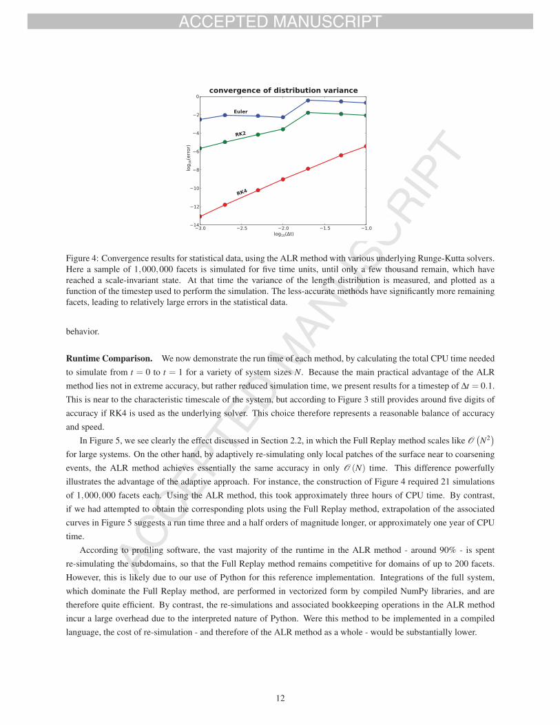
Convergence: statistical measures. A primary aim of large ensemble simulations is the collection of statistics, so

we also wish to demonstrate the convergence of some representative statistical property. The mean facet length is a

quantity of obvious interest, but because the total interface length is conserved, the mean facet length varies discretely

with the number of remaining facets, and is therefore a poor choice for convergence studies. However, subsequent

moments of the facet length distribution are continuous functions of the facet lengths. We therefore present in Figure 4

results on the convergence of the variance of the distribution, illustrating that statistics as well as individual variables

are affected by the numerical error associated with discontinuities. Here, using the now-validated ALR method, we ran

simulations beginning with 1,000,000 facets for five time units, by which time only a few thousand facets remained,

which had achieved scale-invariant behavior. Examining the dependence of the variance of this distribution on the

timestep, we see the same behavior as for the individual facet lengths. Skewness, kurtosis, etc. all display similar

11

Euler

RK2

RK4

log10( t)

log 1

0(error)

convergence of distribution variance

Figure 4: Convergence results for statistical data, using the ALR method with various underlying Runge-Kutta solvers.Here a sample of 1,000,000 facets is simulated for five time units, until only a few thousand remain, which havereached a scale-invariant state. At that time the variance of the length distribution is measured, and plotted as afunction of the timestep used to perform the simulation. The less-accurate methods have significantly more remainingfacets, leading to relatively large errors in the statistical data.

behavior.

Runtime Comparison. We now demonstrate the run time of each method, by calculating the total CPU time needed

to simulate from t = 0 to t = 1 for a variety of system sizes N. Because the main practical advantage of the ALR

method lies not in extreme accuracy, but rather reduced simulation time, we present results for a timestep of Δt = 0.1.

This is near to the characteristic timescale of the system, but according to Figure 3 still provides around five digits of

accuracy if RK4 is used as the underlying solver. This choice therefore represents a reasonable balance of accuracy

and speed.

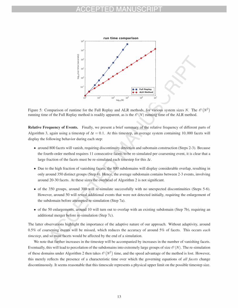
In Figure 5, we see clearly the effect discussed in Section 2.2, in which the Full Replay method scales like O(N2

)for large systems. On the other hand, by adaptively re-simulating only local patches of the surface near to coarsening

events, the ALR method achieves essentially the same accuracy in only O (N) time. This difference powerfully

illustrates the advantage of the adaptive approach. For instance, the construction of Figure 4 required 21 simulations

of 1,000,000 facets each. Using the ALR method, this took approximately three hours of CPU time. By contrast,

if we had attempted to obtain the corresponding plots using the Full Replay method, extrapolation of the associated

curves in Figure 5 suggests a run time three and a half orders of magnitude longer, or approximately one year of CPU

time.

According to profiling software, the vast majority of the runtime in the ALR method - around 90% - is spent

re-simulating the subdomains, so that the Full Replay method remains competitive for domains of up to 200 facets.

However, this is likely due to our use of Python for this reference implementation. Integrations of the full system,

which dominate the Full Replay method, are performed in vectorized form by compiled NumPy libraries, and are

therefore quite efficient. By contrast, the re-simulations and associated bookkeeping operations in the ALR method

incur a large overhead due to the interpreted nature of Python. Were this method to be implemented in a compiled

language, the cost of re-simulation - and therefore of the ALR method as a whole - would be substantially lower.

12

ALR MethodFull Replay

log10(N)

log 1

0(ru

n tim

e [s

econ

ds])

run time comparison

Figure 5: Comparison of runtime for the Full Replay and ALR methods, for various system sizes N. The O(N2

)running time of the Full Replay method is readily apparent, as is the O (N) running time of the ALR method.

Relative Frequency of Events. Finally, we present a brief summary of the relative frequency of different parts of

Algorithm 3, again using a timestep of Δt = 0.1. At this timestep, an average system containing 10,000 facets will

display the following behavior during each step:

• around 800 facets will vanish, requiring discontinuity detection and subomain construction (Steps 2-3). Because

the fourth-order method requires 11 consecutive facets to be re-simulated per coarsening event, it is clear that a

large fraction of the facets must be re-simulated each timestep for this Δt.

• Due to the high fraction of vanishing facets, the 800 subdomains will display considerable overlap, resulting in

only around 350 distinct groups (Step 4). Hence, the average subdomain contains between 2-3 events, involving

around 20-30 facets. At these sizes the overhead of Algorithm 2 is not significant.

• of the 350 groups, around 300 will re-simulate successfully with no unexpected discontinuities (Steps 5-6).

However, around 50 will reveal additional events that were not detected initially, requiring the enlargement of

the subdomain before attempted re-simulation (Step 7a).

• of the 50 enlargements, around 10 will turn out to overlap with an existing subdomain (Step 7b), requiring an

additional merger before re-simulation (Step 7c).

The latter observations highlight the importance of the adaptive nature of our approach. Without adaptivity, around

0.5% of coarsening events will be missed, which reduces the accuracy of around 5% of facets. This occurs each

timestep, and so most facets would be affected by the end of a simulation.

We note that further increases in the timestep will be accompanied by increases in the number of vanishing facets.

Eventually, this will lead to percolation of the subdomains into extremely large groups of size O (N). The re-simulation

of these domains under Algorithm 2 then takes O(N2

)time, and the speed advantage of the method is lost. However,

this merely reflects the presence of a characteristic time over which the governing equations of all facets change

discontinuously. It seems reasonable that this timescale represents a physical upper limit on the possible timestep size.

13

5 Conclusions and Future Work

We have presented a numerical scheme named Adaptive Localized Replay for the integration of coarsening dynamical

systems, which achieves high-order accuracy without the poor scaling performance typical of traditional algorithms

for integrating differential equations with discontinuities. For a fixed number of CPU cycles, our approach can perform

much more accurate simulations than Algorithm #1, resulting in a significant reduction in numerical error; or much

larger simulations than Algorithm #2, resulting in a significant reduction in statistical error. This combination of

benefits should be of particular interest to the coarsening community, where very large ensembles must be simulated

as rapidly as possible, without too much numerical error. By providing high-order accuracy in O (N ) time, our

method should significantly enhance practitioners’ ability to conduct exactly this kind of simulation.

Although our algorithm was developed in the context of faceted surface evolution, it is not specific to that particular

application. The ordered nature of a collection of facets makes the neighbor structure easy to visualize, and is therefore

an ideal first application of the ideas. However, the algorithm should be applicable to any system of discontinuous

ODEs for which the right-hand side of the equation has a sparse neighbor structure, i.e, where the number of “neigh-

bors” of each element does not scale with the system size. For our demonstration problem, regardless of the number

of facets being considered, the velocity function of each facet depends only on two neighboring facets, clearly meeting

this requirement. However, many problems of physical interest can be described by systems of discontinuous ODEs

with only local, and therefore sparse, connectivity structures, and we anticipate that our approach will generalize to

such problems in a straightforward manner.

The system of Equations (5), although associated with a specific physical problem, is interesting primarily as a

simple model system in which the essential features of the algorithm could be clearly expressed. Future work will

include the extension to systems of broader general interest, each with its own specific complicating details. For

instance, the reduced ODE system associated with the Cahn-Hilliard equations of phase separation, written in the

form (3), have a second-nearest-neighbor structure [32, 33]; an analysis similar to that in Sec. 3.1 would reveal that

twice as many facets must be re-simulated per domain to retain solver-level accuracy. On the other hand, the reduced

ODE system associated with the convective Cahn-Hilliard equation, in Eq. (4), has a right hand side that diverges as

facets shrink to zero size [13, 8]; facets therefore exhibit a singular approach to zero, requiring more careful work

to obtain good estimates of the coarsening time. Finally, this method could also be extended to higher-dimensional

surfaces, with a wider variety of events to detect [24]. There, the complication would be that facets on such surfaces

no longer have a unique ordering, and so the concept of “neighbors” must be generalized. These are all tractable

extensions of the present work, but they shall not be pursued here.

Acknolwledgements. SAN thanks Daniel Reynolds and Larry Shampine for many helpful discussions. ST acknowl-

edges the support of an SMU Undergraduate Research Assistantship.

14

References

[1] J. Villain. Continuum models of crystal growth from atomic beams with and without desorption. Journal de

Physique I (France), 1:19–42, 1991.

[2] A. A. Golovin, S. H. Davis, and A. A. Nepomnyashchy. A convective Cahn-Hilliard model for the formation of

facets and corners in crystal growth. Physica D, 122:202–230, 1998.

[3] P. Politi, G. Grenet, A. Marty, A. Ponchet, and J. Villain. Instabilities in crystal growth by atomic or molecular

beams. Physics Reports, 324:271–404, 2000.

[4] T. V. Savina, A. A. Golovin, S. H. Davis, A. A. Nepomnyashchy, and P. W. Voorhees. Faceting of a growing

crystal surface by surface diffusion. Phys. Rev. E, 67:021606, 2003.

[5] A. van der Drift. Evolutionary selection, a principle governing growth orientation in vapor-deposited layers.

Philips Research Reports, 22:267–288, 1967.

[6] A. N. Kolmogorov. To the "geometric selection" of crystals. Dokl. Acad. Nauk. USSR, 65:681–684, 1940.

[7] M. E. Gurtin and P. W. Voorhees. On the effects of elastic stress on the motion of fully faceted interfaces. Acta

Materialia, 46(6):2103–2112, 1998.

[8] S. J. Watson, F. Otto, B. Y. Rubinstein, and S. H. Davis. Coarsening dynamics of the convective Cahn-Hilliard

equation. Physica D, 178(3-4):127–148, April 2003.

[9] S. A. Norris and S. J. Watson. Geometric simulation and surface statistics of coarsening faceted surfaces. Acta

Materialia, 55:6444–6452, 2007.

[10] S. A. Norris, S. H. Davis, P. W. Voorhees, and S. J. Watson. Faceted interfaces in directional solidification.

Journal of Crystal Growth, 310:414–427, 2008.

[11] L. Pfeiffer, S. Paine, G. H. Gilmer, W. van Saarloos, and K. W. West. Pattern formation resulting from faceted

growth in zone-melted thin films. Phys. Rev. Lett., 54(17):1944–1947, 1985.

[12] D. K. Shangguan and J. D. Hunt. Dynamical study of the pattern formation of faceted cellular array growth.

Journal of Crystal Growth, 96:856–870, 1989.

[13] C. L. Emmot and A. J. Bray. Coarsening dynamics of a one-dimensional driven Cahn-Hilliard system. Phys.

Rev. E, 54(5):4568–4575, 1996.

[14] C. Wild, N. Herres, and P. Koidl. Texture formation in polycrystalline diamond films. J. Appl. Phys., 68(3):973–

978, 1990.

[15] J. M. Thijssen, H. J.F. Knops, and A. J. Dammers. Dynamic scaling in polycrystalline growth. Phys. Rev. B,

45(15):8650–8656, 1992.

[16] Paritosh, D. J. Srolovitz, C. C. Battaile, and J. E. Butler. Simulation of faceted film growth in two dimensions:

Microstructure, morphology, and texture. Acta Materialia, 47(7):2269–2281, 1999.

[17] J. Zhang and J. B. Adams. FACET: a novel model of simulation and visualization of polycrystalline thin film

growth. Modeling Simul. Mater. Sci. Eng, 10:381–401, 2002.

15

[18] J. Zhang and J. B. Adams. Modeling and visualization of polycrystalline thin film growth. Computational

Materials Science, 31(3-4):317–328, November 2004.

[19] J. M. Thijssen. Simulations of polycrystalline growth in 2+1 dimensions. Phys. Rev. B, 51(3):1985–1988, 1995.

[20] S. Barrat, P. Pigeat, and E. Bauer-Grosse. Three-dimensional simulation of CVD diamond film growth. Diamond

and Related Materials, 5:276–280, 1996.

[21] G. Russo and P. Smereka. A level-set method for the evolution of faceted crystals. SIAM Journal of Scientific

Computing, 21(6):2073–2095, 2000.

[22] P. Smereka, X. Li, G. Russo, and D. J. Srolovitz. Simulation of faceted film growth in three dimensions: Mi-

crostructure, morphology, and texture. Acta Materialia, 53:1191–1204, 2005.

[23] S. J. Watson and S. A. Norris. Scaling theory and morphometrics for a coarsening multiscale surface, via a

principle of maximal dissipation. Phys. Rev. Lett., 96:176103, 2006.

[24] S.A. Norris and S. J. Watson. Simulating the kinematics of completely faceted surfaces. Journal of Computa-

tional Physics, 231:4560–4577, 2012.

[25] J. E. Taylor and J. W. Cahn. Diffuse interfaces with sharp comers and facets: Phase field models with strongly

anisotropic surfaces. Physica D, 112:381–411, 1998.

[26] J. J. Eggleston, G. B. McFadden, and P. W. Voorhees. A phase-field model for highly anisotropic interfacial

energy. Physica D, 150(1-2):91–103, March 2001.

[27] Colin Ophus, Erik Luber, and David Mitlin. Simulations of faceted polycrystalline thin films: Asymptotic

analysis. Acta Materialia, 57:1327?1336, 2009.

[28] M. Seigert. Coarsening dynamics of crystalline thin films. Phys. Rev. Lett., 81(25):5481–5484, 1998.

[29] A. A. Golovin, S. H. Davis, and A. A. Nepomnyashchy. Model for faceting in a kinetically controlled crystal

growth. Phys. Rev. E, 59:803–825, 1999.

[30] Sofia Biagi, Chaouqi Misbah, and Paolo Politi. Coarsening scenarios in unstable crystal growth. Physical Review

Letters, 109:096101, 2012.

[31] J. W. Cahn and J. E. Hilliard. Free energy of a nonuniform system. I. Interfacial free energy. J. Chem Phys,

28:258, 1958.

[32] K. Kawasaki and T Ohta. Kink dynamics in one-dimensional nonlinear systems. Physica A, 116:573–593, 1982.

[33] T. Kawakatsu and T. Munakata. Kink dynamics in a one-dimensional conserved tdgl system. Progress of

Theoretical Physics, 74:11–19, 1985.

[34] P. W. Bates and J. Xun. Metastable patterns for the cahn-hilliard equation, Part II. layer dynamics and slow

invariant manifold. Journal of Differential Equations, 117:165–216, 1995.

[35] S. A. Norris and S. J. Watson. A mean field theory for coarsening faceted surfaces. Phys. Rev. E, 85:021608,

2012.

[36] L. F. Shampine. Interpolation for runge-kutta methods. SIAM Journal on Numerical Analysis, 22:1014–1027,

1985.

16

[37] E. Hairer, S.P. Nørsett, and G. Wanner. Solving Ordinary Differential Equations I: Nonstiff Problems. Springer,

2009.

[38] Scott A. Norris. Evolving Faceted Surfaces: from continuum modeling, to geometric simulation, to mean-field

theory. PhD thesis, Northwestern University, Evanston, IL, 2006.

17