Adaptive optics for structured illumination microscopy

Adaptive optics for structuredillumination microscopy

Delphine Debarre, Edward J. Botcherby, Martin J. Booth*and Tony Wilson

Department of Engineering Science, University of Oxford, Parks Road, Oxford, OX1 3PJ,United Kingdom.

[email protected]

Abstract: We implement wave front sensor-less adaptive optics in a struc-tured illumination microscope. We investigate how the image formationprocess in this type of microscope is affected by aberrations. It is found thataberrations can be classified into two groups, those that affect imaging ofthe illumination pattern and those that have no influence on this pattern. Wederive a set of aberration modes ideally suited to this application and usethese modes as the basis for an efficient aberration correction scheme. Eachmode is corrected independently through the sequential optimisation of animage quality metric. Aberration corrected imaging is demonstrated usingfixed fluorescent specimens. Images are further improved using differentialaberration imaging for reduction of background fluorescence.

© 2008 Optical Society of AmericaOCIS codes: (010.1080) Adaptive Optics; (010.7350) Wave-front sensing; (180.2520) Fluo-rescence microscopy;(180.6900) Three-dimensional microscopy.

References and links1. J. B. Pawley, ed., Handbook of Biological Confocal Microscopy, 3rd Edition (Springer, New York, 2006).2. J. A. Conchello and J. W. Lichtman, “Optical sectioning microscopy,” Nature Methods 2(12), 920–931 (2005).3. M. A. A. Neil, R. Juskaitis, and T. Wilson, “Method of obtaining optical sectioning by using structured light in a

conventional microscope,” Opt. Lett. 22, 1905–1907 (1997).4. M. J. Booth, “Adaptive optics in microscopy,” Philos. Transact. A Math. Phys. Eng. Sci. 365, 2829–2843 (2007).5. M. J. Booth, M. A. A. Neil, R. Juskaitis, and T. Wilson, “Adaptive aberration correction in a confocal micro-

scope,” Proc. Nat. Acad. Sci. 99, 5788–5792 (2002).6. D. Debarre, M. J. Booth, and T. Wilson, “Image based adaptive optics through optimisation of low spatial fre-

quencies,” Opt. Express 15, 8176–8190 (2007).7. H. Hopkins, “The use of diffraction-based criteria of image quality in automatic optical design,” Opt. Acta 13,

343–69 (1966).8. D. Karadaglic and T. Wilson, “Image formation in structured illumination wide-field fluorescence microscopy,”

Micron (2008, in press).9. E. W. Weisstein, CRC Concise Encyclopedia of Mathematics (Chapman and Hall/CRC, 2003).

10. M. A. A. Neil, M. J. Booth, and T. Wilson, “New modal wavefront sensor: a theoretical analysis,” J. Opt. Soc.Am. A 17, 1098–1107, (2000).

11. M. J. Booth, T. Wilson, H.-B. Sun, T. Ota, and S. Kawata, “Methods for the characterisation of deformablemembrane mirrors,” Appl. Opt. 44(24), 5131–5139 (2005).

12. A. Leray and J. Mertz, “Rejection of two-photon fluorescence background in thick tissue by differential aberra-tion imaging,” Opt. Express 14, 10,565–10,573 (2006).

1. Introduction

Optical sectioning microscopy is widely used to provide three-dimensional fluorescence imagesof biological specimens. A common way of obtaining this sectioning ability is through point

#94950 - $15.00 USD Received 11 Apr 2008; revised 30 May 2008; accepted 3 Jun 2008; published 9 Jun 2008

(C) 2008 OSA 23 June 2008 / Vol. 16, No. 13 / OPTICS EXPRESS 9290

scanning methods such as confocal or multiphoton microscopy [1, 2]. An alternative is to use awide-field technique such as structured illumination (SI) microscopy, which retains the section-ing ability of confocal microscopy, but can be implemented in a conventional microscope usingan incoherent light source, and without the need for scanning [3]. In this technique, the imageof a grid is projected on the specimen so as to produce a one-dimensional sinusoidal excitationpattern in the focal plane of the objective lens. The resulting fluorescence image, consisting ofboth in-focus and out-of-focus fluorescence emission, is acquired by a camera. Several imagesare taken, each corresponding to a different grid position. As the grid pattern appears only in thefocal plane, it is possible to extract an optical section from the spatially modulated componentof the images via a simple calculation.

As with all microscopes, aberrations also detrimentally affect imaging in SI microscopy,leading to lower image intensity and reduced resolution. Image quality can be restored using thetechniques of adaptive optics, where an adaptive element, such as a deformable mirror (DM), isused to correct the aberrations [4]. Traditional adaptive optics systems use a wavefront sensorto measure aberrations. An alternative approach is to use model-based, wavefront sensor-lessschemes, in which the aberration correction is indirectly optimised through the application of ashort sequence of trial aberrations. By using an appropriate combination of optimisation metric,modal aberration expansion and aberration estimator algorithm, correction can be achievedwith a minimal number of measurements. The use of these efficient correction schemes is ofparticular interest in biological imaging, where the reduced number of measurements minimisesphotobleaching and damage on the sample. Such schemes have been demonstrated in confocalmicroscopy [5] and more recently in incoherent transmission imaging [6].

In this paper we describe wavefront sensorless adaptive optics implemented in a SI micro-scope. In Section 2, we study the image formation process in the SI microscope and investigatethe effects of aberrations on imaging performance. It is shown that the final image quality de-pends predominantly on the imaging efficiency of the illumination pattern’s spatial frequency.This imaging efficiency is affected much more by some aberration modes than by others. Conse-quently, different aberration modes can have significantly different effects on the final sectionedimage. We therefore present in Section 3 a general method that provides an optimum modal ex-pansion of the aberration and suggests an efficient aberration correction scheme. In Sections 4to 6, we apply this method to the SI microscope and show how an optimum set of aberrationmodes can be derived theoretically and confirmed experimentally. In the subsequent sections,we describe how the adaptive optics scheme was implemented and applied to the correction ofaberrations in biological specimens. We discuss how the general scheme presented in this papercan be applied to other adaptive optics systems.

2. Image formation in a structured illumination microscope

A structured illumination fluorescence microscope can be modelled as a two stage incoherentimaging system. In such a system, the image I(n) is formed as the convolution of the objectfunction f (n) and the intensity point spread function in the focal plane h(n):

I(n) = h(n)∗ f (n) , (1)

where n is the coordinate vector in the plane perpendicular to the optical axis, and ∗ is theconvolution operation. Alternatively, we can consider the imaging process in the frequencydomain and write:

I(n) = FT−1 [H(m)F(m)] , (2)

where FT is the Fourier transform operation, m is the two-dimensional spatial frequency co-ordinate vector, H(m) is the optical transfer function (OTF), which is equivalent to the two-dimensional FT of h(n), and F(m) is the FT of f (n). For simplicity, we present here expressions



that describe the imaging of two-dimensional objects, but this approach is readily extendable tothree-dimensional imaging. The OTF can be calculated as the autocorrelation of the effectivepupil function, P(r):

H(m) = P(r)⊗P∗(r) =1A

∫∫

D(m)

P(r−m)P∗(r)dA , (3)

where ⊗ is the correlation operation, A is the pupil area, r is the position vector, P ∗ is thecomplex conjugate of P and D(m) is the region of overlap of the offset pupils. We assume acircular pupil with unity radius, so D(m) is defined by |r| ≤ 1 and |r−m| ≤ 1 (see Fig. 1, partb1). If there is no amplitude variation across the pupil, then we can express P(r) = exp [ jΦ(r)],where Φ(r) is the phase aberration and j =

√−1. The OTF becomes

H(m) =1π

∫∫

D(m)

exp [ jΔΦ(m,r)]dr (4)

withΔΦ(m,r) = Φ(r−m)−Φ(r) . (5)

The aberration difference function ΔΦ(m,r), rather than the aberration Φ(r), is therefore theimportant quantity when considering the effect of aberrations in the incoherent imaging of aparticular spatial frequency m [7].

The SI microscope relies upon the projection of a physical grid pattern into the focal planeof the specimen. We assume that the grid object is a sinusoidal transmission mask with unitymodulation depth and spatial frequency vector g, of the form 1+cos(ψ + g.n). The variable ψis the spatial phase shift of the pattern that depends on the grid displacement along the directionof g. Using equation 2, the excitation pattern formed by its image in the specimen can thus bewritten as:

Iexc(n) = Hexc(0)+Hexc(g)e( jψ+ jg.n)

2+Hexc(-g)

e−( jψ+ jg.n)

2, (6)

where Hexc(m) is the FT of hexc(r), the intensity PSF of the excitation path imaging system.This illumination pattern excites fluorescence in the specimen, whose fluorophore distributionis described by the object function f (n). The generated fluorescence is therefore given by theproduct f (n)Iexc(n). If we now consider the image Ii(n) of this fluorescence obtained on thecamera for a position i of the grid corresponding to ψ = ψ i, we can write

Ii(n) = [ f (n)Iexc,i(n)]∗ hem(n) , (7)

where hem(n) is the intensity PSF of the emission path of the microscope. For simplicity, weassume from here on that the excitation and emission wavelengths are close and that the aber-rations are equal for the excitation and the emission pathways. Hence h exc(n) = hem(n) = h(n)and equivalently Hexc(m) = Hem(m) = H(m).

The sectioned image is retrieved from the three images I i(n) corresponding to grid positionsψi = 0, 2π

3 and 4π3 respectively, using the formula [3]:

Isect(n) =√

∑i�= j

(Ii − I j)2 . (8)

It can be shown that this image, when expressed in terms of spatial frequencies, is given by [8]:

Isect(n) =32

∣∣H(g)FT−1 [F(m)H(g+ m)]∣∣ . (9)



b1

g

D ( g )

-Φ(r)

(r-g)

gx

gy

gx

gy

gx

gy

b2

b3

c1

c2

c3

d1

d2

d3

e1

e2

e3

(r,g)

P*

Pa1

a2

a3

0

1

Image

intensity (a.u.)-4

4 Phase (rad)

ΔΦ

Φ

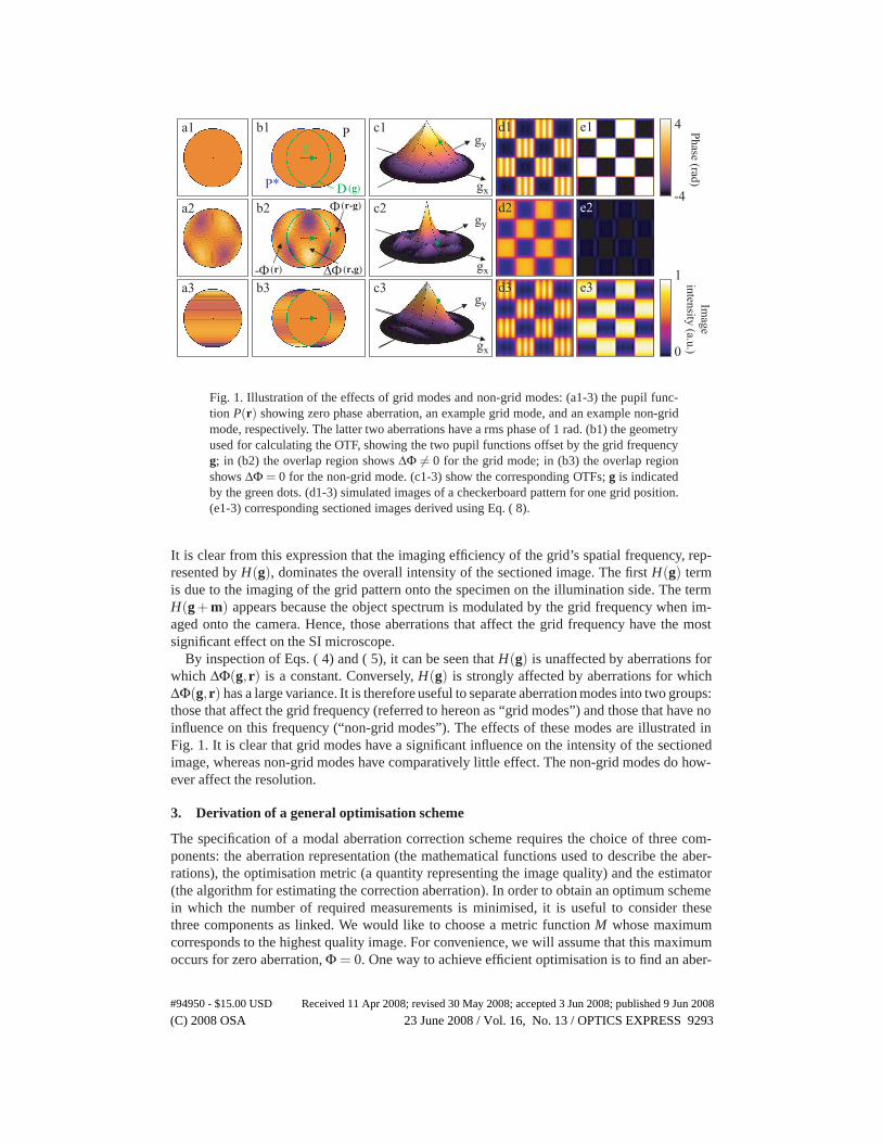
Fig. 1. Illustration of the effects of grid modes and non-grid modes: (a1-3) the pupil func-tion P(r) showing zero phase aberration, an example grid mode, and an example non-gridmode, respectively. The latter two aberrations have a rms phase of 1 rad. (b1) the geometryused for calculating the OTF, showing the two pupil functions offset by the grid frequencyg; in (b2) the overlap region shows ΔΦ �= 0 for the grid mode; in (b3) the overlap regionshows ΔΦ = 0 for the non-grid mode. (c1-3) show the corresponding OTFs; g is indicatedby the green dots. (d1-3) simulated images of a checkerboard pattern for one grid position.(e1-3) corresponding sectioned images derived using Eq. ( 8).

It is clear from this expression that the imaging efficiency of the grid’s spatial frequency, rep-resented by H(g), dominates the overall intensity of the sectioned image. The first H(g) termis due to the imaging of the grid pattern onto the specimen on the illumination side. The termH(g + m) appears because the object spectrum is modulated by the grid frequency when im-aged onto the camera. Hence, those aberrations that affect the grid frequency have the mostsignificant effect on the SI microscope.

By inspection of Eqs. ( 4) and ( 5), it can be seen that H(g) is unaffected by aberrations forwhich ΔΦ(g,r) is a constant. Conversely, H(g) is strongly affected by aberrations for whichΔΦ(g,r) has a large variance. It is therefore useful to separate aberration modes into two groups:those that affect the grid frequency (referred to hereon as “grid modes”) and those that have noinfluence on this frequency (“non-grid modes”). The effects of these modes are illustrated inFig. 1. It is clear that grid modes have a significant influence on the intensity of the sectionedimage, whereas non-grid modes have comparatively little effect. The non-grid modes do how-ever affect the resolution.

3. Derivation of a general optimisation scheme

The specification of a modal aberration correction scheme requires the choice of three com-ponents: the aberration representation (the mathematical functions used to describe the aber-rations), the optimisation metric (a quantity representing the image quality) and the estimator(the algorithm for estimating the correction aberration). In order to obtain an optimum schemein which the number of required measurements is minimised, it is useful to consider thesethree components as linked. We would like to choose a metric function M whose maximumcorresponds to the highest quality image. For convenience, we will assume that this maximumoccurs for zero aberration, Φ = 0. One way to achieve efficient optimisation is to find an aber-



ration expansion for which the modes act independently on the metric. This would allow theindependent optimisation of each mode. This can be achieved if the metric is of the form

M = M0 −∑i

x2i , (10)

where M0 is the value of the metric for zero aberration and the coefficients x i represent aberra-tion mode amplitudes. When M is expressed in this form, it is clear that independent maximisa-tion with respect to each xi is possible. Furthermore, as the function is quadratic, the maximumcan be found directly from three measurements of M corresponding to three different valuesof xi [6]. In practice, these measurements would be taken with three different trial aberrationsintroduced by the correction element. However, M only takes the form shown in Eq. ( 10) ifthe aberration representation is appropriately chosen. In this section we explain a generallyapplicable process that facilitates this choice.

Let us assume that the aberrations are represented by an expansion over a complete (butas yet undefined) set of modes {Xi} with a set of coefficients {ai} so that Φ = ∑i aiXi. It isalso convenient to represent this aberration as a vector a, whose elements are the coefficients{ai}. In general, for sufficiently small aberrations, M would be approximated by a quadraticpolynomial:

M ≈ M0 −∑i

∑j

αi jaia j = M0 −aT Aa , (11)

where the constants αi j are the elements of the matrix A. In this form, the combination of themetric and the aberration expansion is not ideal for efficient optimisation as the coefficientsdo not act independently. As this expression represents a maximum of M, the matrix A mustbe positive semi-definite, i.e. aTAa ≥ 0 for all a �= 0. Furthermore, any positive semi-definitematrix can be converted into a diagonal matrix by:

A = VBVT , (12)

where B is a diagonal matrix with elements Bii = βi and where the columns of the orthogonalmatrix V are the eigenvectors of A. Naturally, the diagonal elements of B are also the eigenval-ues of A. The optimisation metric then becomes

M ≈ M0 −aT VBVT a = M0 −bT Bb = M0 −∑i

βib2i , (13)

with b = VTa. Eq. ( 13) has the desired form shown in Eq. ( 10). The process of convertingEq. ( 11) into the form of Eq. ( 13) is equivalent to obtaining an alternative expansion of theaberration function in terms of a new set of modes {Yi} so that Φ = ∑i biYi, where the newmodes can be calculated as Yi = ∑ j Vi jXj.

We now outline the procedure for obtaining the matrix A. As this is a positive semi-definitematrix, it must also be equivalent to a Gram matrix (the matrix of inner products of a particularset of basis functions) [9]. It follows that A can be calculated if one has an appropriate definitionfor the inner product, α i j =

⟨Xi,Xj

⟩. This can sometimes be obtained from an expansion of the

metric M in terms of the aberration coefficients ai. This process is illustrated in the followingsections. Alternatively, A can be determined empirically, by measuring the behaviour of M inthe vicinity of the maximum. This process is demonstrated in Section 6.

We note that the metric M may be insensitive to certain aberration modes and therefore themaximum value may also occur for other values of Φ �= 0 (as an example, measurements in mostmicroscopes would be insensitive to a constant phase offset). Equivalently, the inner productwould be degenerate, meaning that 〈Yi,Yi〉 = 0 for certain i. This property is useful as it enablesthe separation of the set of aberration modes into those that affect the chosen metric and those



that have no influence. In the latter case, the expression in Eq. ( 13) would contain zero valuesfor each βi corresponding to a mode Yi that did not influence the metric. Clearly, it would notbe desirable to include these modes in any correction scheme.

4. Optimisation metric for structured illumination microscopy

A commonly used function that satisfies the required properties of an optimisation metric is theimage sharpness, defined as:

M =∫∫ +∞

−∞I2sect(n)dn . (14)

With the help of Eq. ( 9) and using Parseval’s theorem, it becomes

M =∫∫

S|F(m)|2 |H(g)H(g+ m)|2 dm , (15)

where we have neglected the premultiplying constant. The region of integration S is the circularregion of support of the offset OTF H(g+m). If we assume that the sample frequency spectrumtakes significant values only for small values of |m| (an approximation valid for many practicalsamples), we obtain using a Taylor expansion (see Appendix B):

M =(∫∫

S|F(m)|2 dm

)|H(g)|4 +

12

(∫∫S|F(m)|2 m2 dm

)|H(g)|2 ∇2

(|H(g)|2

), (16)

where ∇2 is the Laplacian operator and where we take ∇2t(g) to mean [∇2m′t(m′)]m′=g. In each

term of this equation, the effects of aberrations are separated from the object properties. Thisenables us to design a correction scheme that is mostly independent of the object structure. Fora given object, the integral terms in parentheses are constants and Eq. ( 16) can be written as

M = F0 |H(g)|4 +F1 |H(g)|2 ∇2(|H(g)|2

), (17)

where F0 and F1 are constants. This equation suggests a two stage scheme for aberration cor-rection in the SI microscope, firstly correcting grid modes and thereafter non-grid modes.

For grid modes, the variation of M is dominated by the first term of Eq. ( 17); non-grid modesby definition have no effect on this term. Hence, following the scheme presented in Section 3,we can determine the appropriate inner product using M ∼ F0 |H(g)|4 and thus derive the set ofgrid modes. The first stage of optimisation is performed using this subset of aberrations.

The remaining aberration then consists solely of non-grid modes, for which we can considerH(g) to be constant. For this second stage of optimisation, the metric therefore varies as M ∼∇2

(|H(g)|2

). This expression can be used to obtain a different inner product from which the

non-grid modes can be derived. We then perform optimisation based upon these modes. In thenext section we derive these two inner products explicitly.

5. Explicit expression of the metric as a function of modal coefficients

For small amplitudes of ΔΦ, the exponential term in Eq. ( 4) can be expanded as a Taylor series,giving

H(m) =1π

∫∫

D(m)

dr+jπ

∫∫

D(m)

ΔΦ(m,r)dr− 12π

∫∫

D(m)

[ΔΦ(m,r)]2 dr . (18)



If M is dominated by the first term in Eq. ( 17), we can write

M =F0

∣∣∣∣∣∣∣H0(g)+

jπ

∫∫

D(g)

ΔΦ(g,r)dr− 12π

∫∫

D(g)

ΔΦ2(g,r)dr

∣∣∣∣∣∣∣

4

, (19)

where H0(g) is the OTF in the absence of aberrations. For a fixed grid frequency, this is aconstant, so will be referred to simply as H0. Considering only terms up to the second order,Eq. ( 19) can be written:

M = F0

{H4

0 −2H20

[H0

π

∫∫

D(g)

[ΔΦ(g,r)]2 dr−(

1π

∫∫

D(g)

ΔΦ(g,r)dr)2]}

(20)

Let the pupil phase be represented by the modal expansion Φ = ∑i aiXi. We define correspond-ing aberration difference modes as ΔXi(g,r) = Xi(r−g)− Xi(r) so that ΔΦ = ∑i aiΔXi. Eq.( 20) then becomes

M = F0

{H4

0 −2H20 ∑

i∑

j

aia j

[H0

π

∫∫

D(g)

ΔXiΔXjdr− 1π2

∫∫

D(g)

ΔXidr∫∫

D(g)

ΔXjdr]}

, (21)

where for brevity we have omitted the arguments of the ΔXi(g,r) terms. Comparison of Eqs.( 11) and ( 21) shows that the expression in square brackets represents the inner product requiredto determine the coefficients αi j. The metric is therefore

M = M0 −∑i

∑j

aia j⟨Xi,Xj

⟩, (22)

where M0 = F0H40 and where the (degenerate) inner product is defined by

⟨Xi,Xj

⟩grid = 2F0H

20

⎡⎢⎣H0

π

∫∫

D(g)

ΔXiΔXjdr− 1π2

∫∫

D(g)

ΔXidr∫∫

D(g)

ΔXjdr

⎤⎥⎦ . (23)

This inner product is used to derive the grid modes when the specimen is a thin object locatedin the focal plane. However in the case of a more realistic sample with finite thickness, the axialextent of the specimen should also be taken into account. Following the same principles, anexpression for such an inner product is derived in Appendix A.

As the inner product 〈 , 〉grid is degenerate for non-grid modes, for the second stage of cor-rection we need another inner product that is derived using the second term of Eq. ( 17). Thegrid pattern in the specimen is unaffected by non-grid modes. It follows that the axial sectioningstrength of the microscope does not vary with the amplitude of these aberrations and, hence,we only need consider the plane z = 0 in the following analysis. It is shown in Appendix B thatthe new inner product is defined, to the lowest order in m, as

⟨Xi,Xj

⟩non−grid = F1

⎡⎢⎣H0

π

∫∫

D(g)

∇X ′i ∇X ′

jdr− 1π2

∫∫

D(g)

∇X ′i dr

∫∫

D(g)

∇X ′jdr

⎤⎥⎦ , (24)

where ∇ is the gradient operator and X ′i represents Xi(r−g).



1.8

0

1.2

0

Z7 Z9 Z10

Z7

Z9

Z10

Y7

Y9

Y10

Y7 Y9 Y10

a

c

b

dφ = γ (sinθ Z9 + cosθ Z10)φ = γ (sinθ Z7 + cosθ Z10)φ = γ (sinθ Z7 + cosθ Z9)

φ = γ (sinθ Y9 + cosθ Y10)φ = γ (sinθ Y7 + cosθ Y10)φ = γ (sinθ Y7 + cosθ Y9)

< Zi , Zj >

< Yi , Yj >

Fig. 2. Experimental determination of aberration modes. (a), the metric M is plotted as afunction of the aberrated phase Φ(r) for a number of basis modes (here 3 Zernike modes:coma (z=7) and trefoil (z=9 and z=10)), and the resulting curves are fitted to a multidimen-sional ellipsoid. (b), the fitting parameters are used to construct the experimental A matrixand determine the new set of modes {Yi(r)}. (c), a similar plot of the metric M, derivedusing the new set of modes. The main axes of the fitted ellipsoid now correspond to pure{Yi(r)} modes. (d), the experimental A matrix for the new modes is diagonal, confirmingthat the cross-talk between the modes has been cancelled. Although only three modes areshown here, this principle can be extended to an arbitrary number.

6. Experimental determination of aberration modes

In order to verify the theoretical derivation, we developed a complementary empirical methodfor ascertaining the optimal set of modes for aberration correction. The method relies on theprinciple outlined in Fig. 2: for any pair (i, j) of initial modes with i �= j, the value of M ismeasured for a number of aberrated pupil phases Φ(r,θ ) obtained by combining the basismodes Xi(r) and Xj(r) with constant amplitude γ :

Φ(r,θ ) = γ cosθ Xi(r)+ γ sinθ Xj(r) , (25)

where θ varies between 0 and 2π . In the vicinity of its maximum, the contours of M as afunction of the coefficients

{ai j

}are ellipsoidal. Therefore, the resulting curves were simulta-

neously fitted to a multidimensional ellipsoid defined as

∑i, j

αi jaia j = c (26)

where c is a constant. This fitting provides us with the coefficients α i j and hence the matrixA. This matrix is identical to that derived in Section 5, but is obtained without recourse to theinner product calculation. The same approach can be used as before to derive the new set ofbasis modes {Yi}. An example of this orthogonalisation process is presented in Fig. 2. Theseresults were obtained using the experimental set-up described in the next section and the valueof the metric M was calculated from images of a thin inhomogeneous fluorescent sheet locatedin the focal plane of the focussing objective, for various values of Φ(r,θ ). In order to test the



4 6 8 10 12 140

1

2

3

FWH

M o

f est

imat

or c

urve

(rad

)

Aberration mode

theory experimenttheory

experiment

theory

experiment

a b

Fig. 3. Set of modes used for aberration correction. (a), set of modes determined experi-mentally and theoretically using an initial set of 11 Zernike modes (z=5 to 15). The modesare ordered by decreasing eigenvalue. The last two modes have no influence on the imagingof the grid. All the modes have a root mean square (rms) phase amplitude of 1 rad. (b), In-fluence of the modes on the metric M, determined theoretically using the mode eigenvalues,and experimentally as the FWHM of the curve of M as a function of aberration amplitudein a single mode. The last two modes influence only the sample frequency spectrum, andhence their eigenvalues depend on the sample and cannot be determined theoretically.

validity of this method, the same process was repeated with the newly determined modes . Weobtained a diagonal matrix, confirming that the new set of modes does not exhibit cross-talkand can be used for sequential correction of the aberrations.

The comparison between the experimentally determined modes and their theoretically de-termined counterparts is presented in Fig. 3. The two sets were obtained using eleven Zernikemodes (z = 5 to z = 15 using the indexing scheme of Reference [10]) as the basis functions{Xi}. We note that piston, tip, tilt and defocus were not used as basis functions as they shouldnot be included in correction schemes for three dimensional imaging to avoid changing theimaged region in the sample. Good agreement was found between the two approaches. The ob-served discrepancies were attributed to the residual error in the control of the aberrated phase inthe pupil plane. It should be noted here that since the derivation was independent of the objectstructure, this characterization was only performed once, and the same set of modes was usedfor all the following experiments.

We measured the variation of M as a function of aberration amplitude for each of the {Y i}modes. These curves were accurately described by Gaussian functions; the full width at halfmaximum (FWHM) for each of the curves is displayed in Fig. 3b. In the case of grid modes,the obtained values can be related to the eigenvalues β i and show a good agreement with thecalculated values. It should be noted that the width of each curve also determines the domainof validity of the quadratic approximation used in section 3, which is approximately the sameas the FWHM. For greater aberration amplitudes, we found experimentally that correction ofeach mode could still be performed independently with good accuracy by taking into accountthe Gaussian shape of the curves in the correction algorithm. The range of the correction wasthus only limited by the aberration amplitude accessible to our DM.

7. Results

We demonstrated the aberration correction scheme in a structured illumination microscopebased around a modified IX70 inverted microscope (Olympus), incorporating a deformable



WLS

DM

DBSBSC

BSC

S

60x, 1.2 NA

180mm80mm

100mm

50mm

200mm

160mm

80mm

100mm

150mm

Lasergrid

Exc. filter

Em. filter

CCD

CCD

Fig. 4. Schematic of the structured illumination microscope with aberration correction.WLS, white light source. DM, deformable mirror. DBS, dichroic beamsplitter. BSC, beam-splitter cube. S, sample. The blue rays mark the illumination path; the detection path isshown in yellow. The green path represents the Mach Zehnder interferometer used to char-acterise the deformable mirror – this is not used during the imaging experiments.

mirror (DM – Boston Micromachines Corp., Multi-DM), a 60x, 1.2NA water objective lenswith coverslip correction (Olympus) and a 30-μm period grid (Optigrid, Thales) (see Fig. 4).With the magnification of our system, the spatial frequency of the grid in the pupil plane wasabout 4 times smaller than the incoherent frequency cutoff, corresponding to a theoretical axialresolution of 0.46 μm [8]. The grid was illuminated by a white-light source with a narrowbandexcitation filter centered on 488 nm (Chroma) and imaged in the focal plane of the objectiveafter being reflected off the DM, which was conjugated to the pupil plane of the objective. Thefluorescence was then detected on a CCD camera through a broadband emission filter and adichroic beamsplitter (both Chroma), after reflection off the DM. In order to precisely controlthe aberrations induced by the DM, an interferometer was added to the set-up, incorporating a532nm laser and a CCD camera conjugated with both the pupil plane of the objective and theDM. By placing a mirror in the focal plane of the objective, this permitted us to measure theaberrated phase in the pupil plane and hence to determine the combinations of control signalssent to the mirror that would produce a given aberration mode [11]. The control signals wererestricted to ensure that the DM operated in a linear range; this range was found to cover ap-proximately 85% of the full deflection of the DM. As the relative position of the mirror and theobjective were fixed, the characterisation was performed only once, and the same control ma-trix was then used in the rest of the experiments. As a final step, we used an appropriate controlsignal offset to ensure the initial flatness of the mirror lay within the measurement uncertaintyof our set-up (rms phase ≤ 0.02 rad).

Using the experimentally determined modes shown in Fig. 3, we performed aberration cor-rection on a fixed mouse intestine sample (FluoCells prepared slide 4, Molecular Probes, USA)using a multi-dimensional quadratic maximization algorithm: for each aberration mode, themetric M was measured when adding a given amount of the considered mode, then again whensubstracting the same amount. Along with the measured value of M when no aberration wasadded, this allowed us to estimate the initial aberration present in each of the assessed modes



0 100.0

0.5

1.0

1.5

Sign

al (a

.u.)

Position (μm)

a b c

10 ∝m 20

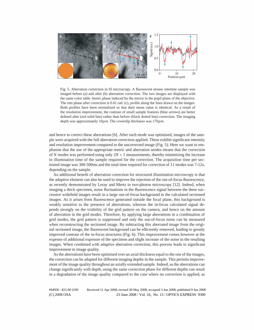
Fig. 5. Aberration correction in SI microscopy. A fluorescent mouse intestine sample wasimaged before (a) and after (b) aberration correction. The two images are displayed withthe same color table. Insert, phase induced by the mirror in the pupil plane of the objective.The rms phase after correction is 0.61 rad. (c), profile along the lines drawn on the images.Both profiles have been normalized so that their mean value is identical. As a result ofthe resolution improvement, the contrast of small sample features (blue arrows) are betterdefined after (red solid line) rather than before (black dotted line) correction. The imagingdepth was approximately 10μm. The coverslip thickness was 170μm.

and hence to correct these aberrations [6]. After each mode was optimised, images of the sam-ple were acquired with the full aberration correction applied. These exhibit significant intensityand resolution improvement compared to the uncorrected image (Fig. 5). Here we want to em-phasise that the use of the appropriate metric and aberration modes means that the correctionof N modes was performed using only 2N +1 measurements, thereby minimizing the increasein illumination time of the sample required for the correction. The acquisition time per sec-tioned image was 300-500ms and the total time required for correction of 11 modes was 7-12s,depending on the sample.

An additional benefit of aberration correction for structured illumination microscopy is thatthe adaptive element can also be used to improve the rejection of the out-of-focus fluorescence,as recently demonstrated by Leray and Mertz in two-photon microscopy [12]. Indeed, whenimaging a thick specimen, noise fluctuations in the fluorescence signal between the three suc-cessive widefield images result in a large out-of-focus background in the calculated sectionedimages. As it arises from fluorescence generated outside the focal plane, this background isweakly sensitive to the presence of aberrations, whereas the in-focus calculated signal de-pends strongly on the visibility of the grid pattern on the camera, and hence on the amountof aberration in the grid modes. Therefore, by applying large aberrations in a combination ofgrid modes, the grid pattern is suppressed and only the out-of-focus noise can be measuredwhen reconstructing the sectioned image. By subtracting this aberrated image from the origi-nal sectioned image, the fluorescent background can be efficiently removed, leading to greatlyimproved contrast of the in-focus structures (Fig. 6). This improvement comes however at theexpense of additional exposure of the specimen and slight increase of the noise in the resultingimages. When combined with adaptive aberration correction, this process leads to significantimprovement in image quality.

As the aberrations have been optimised over an axial thickness equal to the one of the images,the correction can be adapted for different imaging depths in the sample. This permits improve-ment of the image quality throughout an axially extended sample. Indeed, as the aberrations canchange significantly with depth, using the same correction phase for different depths can resultin a degradation of the image quality compared to the case where no correction is applied, as



0 5 10 15 200.0

0.5

1.0

d

e

a

Sig

nal (

a.u.

)

position ( m)

b

Fluorescence signal (a.u.)

1

0Pha

se in

trod

uced

(ra

d) 10

-10

f

a b c

d = a - c e = b - c

10 m

Fig. 6. Aberration correction and out-of-focus fluorescence rejection in SI microscopy. Ax-ially sectioned images of a pollen grain without (a) and with (b) aberration correction,and with large induced aberration (c). The phase induced by the mirror is shown as aninsert. In (c), the phase was a combination of the first 4 aberration modes in Fig. 3 withtotal rms amplitude of 3 radians. Background-free images were obtained by subtractingthe highly aberrated image (c) from the images obtained before and after aberration cor-rection, giving (d) and (e) respectively. (f), profiles obtained along the line drawn in (b)for images (a),(b),(d) and (e): aberration correction increases the intensity of the structureswhile background subtraction improves the contrast. The imaging depth was approximately30μm. The coverslip thickness was 170μm.

demonstrated in Fig. 7.

8. Discussion and conclusion

We have shown that the image formation in SI microscopy is strongly dependent upon aberra-tion modes that affect the imaging of the grid frequency. These grid modes cause a significantreduction in the intensity of the sectioned image and lower resolution. Conversely, non-gridmodes have little effect on the final image intensity. It is important to note that both of thesesets of modes would strongly affect the imaging quality in confocal and other sectioning mi-croscopes. We are therefore led to the conclusion that the SI microscope, in comparison toother sectioning microscopes, is more susceptible to certain aberrations (grid modes) and moreresilient to others (non-grid modes).

Whilst the SI microscope relies upon a relatively simple optical principle, the image for-mation process has a complex mathematical description. Similarly, the derivation of a model-based, sensorless, adaptive optical scheme is a complex process. However, our results show thatthe scheme is effective in correcting specimen-induced and system aberrations and restoringimage quality. For the samples presented here, we found that the aberration mainly consisted of



a b c

d e f

10 m

Fig. 7. Correction variation with imaging depth. Pollen grain images after background sub-traction, at the top of the grain (a,b and c) and around the equator 20μm below (d,e and f).The images were acquired without aberration correction (a and d), with the correction op-timised for the top of the grain (b and e), and for the equator (c and f). Images in the samerow are displayed with the same color code and the phase induced by the DM is shownas an insert. The appropriate correction settings for one plane (b and f) clearly deterioratethe image quality in another plane (c and e). The rms phase after correction is 0.37 rad in(b) and 0.63 rad in (c). The imaging depth was approximately 30− 50μm. The coverslipthickness was 170μm.

astigmatism, coma and spherical aberration modes. The magnitude of the astigmatism compo-nent was similar across various samples, suggesting that it arises from our optical system. Theamplitude of coma and spherical aberration, however, varied significantly across different sam-ples, or at various depth inside the same sample (see Fig. 7), indicating that these aberrationsare induced by the specimens.

The adaptive scheme described here has significant advantages over model-free algorithms inthat the aberration correction can be estimated using a small number of measurements (2N +1for N aberration modes). Moreover, as the scheme is mostly independent of the object structure,the appropriate modes have only to be determined once and the same scheme can be used forany specimen. We have also shown that aberration correction can be effectively combined withbackground subtraction to further improve SI microscope images. In the results presented here,aberration correction was performed as an average over an image frame and therefore wouldnot correct for any local variations in aberrations. If these variations were found to be signif-icant, the image could be formed from several sub-images for which independent aberrationcorrection would be performed.

We have presented a general method that provides an optimal aberration expansion for achosen optimisation metric. This relied upon the derivation of an inner product from a mathe-matical model of the imaging process, followed by an orthogonalisation process applied to a setof basis functions, such as the Zernike functions. This process reveals a wealth of informationabout the effects of different aberration modes on an imaging system – for the SI microscope,it enabled us to derive the sets of grid modes and non-grid modes. This method could equallybe applied to any sectioning microscope to derive aberration expansions that are best suited tothat application.



Acknowledgments

D. Debarre was supported by the Delegation Generale pour l’Armement and the Human Fron-tier Science Program. M. J. Booth was a Royal Academy of Engineering/EPSRC ResearchFellow. This work was supported by a grant from the Royal Society.

Appendix A: Inner product for grid modes with a three-dimensional specimen

In order to take into account the axial extension of the sample, we introduce the parameter zas the axial distance between the considered plane and the focal plane. With this notation, theincoherent OTF can be generalized as:

H(m,z) =1π

∫∫

D(g)

exp [ jΔΦ(g,r)+ jΔΦd(g,r,z)]dr , (27)

with ΔΦd(g,r,z) = az(|r−g|2 − r2)/2 and a = (8πn/λ )sin2 (α/2) and where nsin(α) is thenumerical aperture of the objective lens and λ is the wavelength in vacuum. Using this expres-sion, the excitation pattern on the sample for each spatial phase shift ψ i is given by:

Iexc,i(n,z) = H(0,z)+H(g,z)e( jψi+ jg.n)

2+H(−g,z)

e−( jψi+ jg.n)

2(28)

The image obtained on the camera is then obtained by integrating the intensity correspondingto different planes in the sample:

Ii(n) =∫ +∞

−∞

{H(0,z)FT−1 [F(m,z)H(m,z)]+

e jψi

2H(g,z)FT−1 [F(m−g,z)H(m,z)]

+e− jψi

2H(-g,z)FT−1 [F(m+ g,z)H(m,z)]

}dz ,

(29)

and accordingly the axially sectioned image can be expressed as:

Isect(n) =32

∣∣∣∣∫ +∞

−∞H(g,z)FT−1 [F(m,z)H(g+ m,z)]dz

∣∣∣∣ . (30)

This can be simplified by assuming that the two-dimensional spatial frequency spectrum of thesample, F(m,z), varies slowly with z at the scale of the axial resolution of the sectioned image,such that we can write F(m,z) ≈ F(m). Under this assumption, Parseval’s theorem yields:

M =∫∫ +∞

−∞I2sect(n)dn ≈

∫∫S|F(m)|2

∣∣∣∣∫ +∞

−∞H(g,z)H(g+ m,z)dz

∣∣∣∣2

dm . (31)

Here we restrict ourselves to grid modes, and hence consider that the effect of aberrations onthe metric is dominated by the changes in the grid pattern intensity. In this case we can writeH(g+ m,z) ≈ H(g,z) and:

M ≈ F0

∣∣∣∣∫ +∞

−∞H(g,z)2dz

∣∣∣∣2

. (32)

For small aberration amplitudes, the optical transfer function can be approximated by a Taylorexpansion, giving:

H(g,z) =1π

∫∫

D(g)

ζ (g,r,z)dr+jπ

∫∫

D(g)

ΔΦ(g,r)ζ (g,r,z)dr− 12π

∫∫

D(g)

ΔΦ(g,r)2ζ (g,r,z)dr (33)



where the defocus term ζ is defined as

ζ (g,r,z) = exp [ jΔΦd(g,r,z)] (34)

From here on, for notational brevity, we omit the explicit dependence of ΔΦ(g,r) and ζ (g,r,z)on their arguments. The first term of Eq. ( 33) corresponds to the defocused OTF in the absenceof aberration; this is denoted as H0 in the following expressions. Introducing H(g,z) into Eq.( 32) yields:

M ≈F0

∣∣∣∣∫ +∞

−∞H2

0 dz

∣∣∣∣2

−F0

{2

π2

∫ +∞

−∞H2

0 dz∫ +∞

−∞

[∫∫

D(g)

ΔΦζdr]2

dz

+2π

∫ +∞

−∞H2

0 dz∫ +∞

−∞H0

∫∫

D(g)

ΔΦ2ζdrdz− 4π2

[∫ +∞

−∞H2

0

∫∫

D(g)

ΔΦζdrdz

]2},

(35)

As a result, the inner product derived from the metric is defined here as:

⟨Xi,Xj

⟩grid z =F0

{2

π2

∫ +∞

−∞H2

0 dz∫ +∞

−∞

[∫∫

D(g)

ΔXiζdr][∫∫

D(g)

ΔXjζdr]dz

+2π

∫ +∞

−∞H2

0 dz∫ +∞

−∞H0

∫∫

D(g)

ΔXiΔXjζdrdz

− 4π2

[∫ +∞

−∞H2

0

∫∫

D(g)

ΔXiζdrdz

][∫ +∞

−∞H2

0

∫∫

D(g)

ΔXjζdrdz

]}(36)

Appendix B: Inner product for non-grid modes

Here we consider non-grid modes, which do not affect the grid pattern projected on the sample.For those aberrations, the sectioning strength is independent of the aberration amplitude, andhence we only need consider the plane z = 0 in the following analysis. Starting with:

M =∫∫

S|F(m)|2 |H(g)H(g+ m)|2 dm , (37)

we assume |F(m)|2 takes significant values only for small m and expand H(g+m) as a Taylorseries up to the second order term [9]:

M =∫∫

S|F(m)|2 |H(g)|2

(|H(g)|2 +(m.∇) |H(g)|2 +

12

[(m.∇)2 |H(g)|2

])dm (38)

where we take (m.∇)t(g) to mean [(m.∇m′)t(m′)]m′=g. If we further assume that the object isreal, then F(-m) = F ∗(m) and hence:

∫∫S|F(m)|2 m dm = 0

∫∫S|F(m)|2 mxmy dm = 0 (39)

We also assume that the object structure (and hence frequencies) are not predominantly alignedwith one direction, so that

∫∫S |F(m)|2 m2

x dm ≈ ∫∫S |F(m)|2 m2

y dm, and we obtain:

M = F0 |H(g)|4 + F1 |H(g)|2 ∇2(|H(g)|2

), (40)



where ∇2 is the Laplacian operator and:

F1 =12

∫∫S|F(m)|2 m2 dm . (41)

Using Eq. ( 18), we find that for small aberration difference amplitudes

|H(g+ m)|2 ≈ |H0(g+ m)|2 − |H0(g+ m)|π

∫∫

D(g+m)

ΔΦ(g+ m,r)2dr+[ 1

π

∫∫

D(g+m)

ΔΦ(g+ m,r)dr]2

(42)

Under the assumption that m is small, we can write:

ΔΦ(g+ m,r) = ΔΦ(g,r)+ Φ(r−g)−Φ(r−g−m)≈ ΔΦ(g,r)+ (m.∇)Φ(r−g) .

(43)

Since we consider only non-grid modes, for all r within D(g), ΔΦ(g,r) = 0. If we consideronly slowly varying phase functions and for small values of m, this is also valid for all r withinD(g+ m), and therefore:

ΔΦ(g+ m,r) ≈ (m.∇)Φ(r−g) . (44)

Equation 42 can be simplified to:

|H(g+ m)|2 ≈ |H0(g+ m)|2 − |H0(g)|π

∫∫

D(g)

[(m.∇)Φ(r−g)]2 dr+[ 1

π

∫∫

D(g)

(m.∇)Φ(r−g)dr]2

(45)

Combining this with Eq. ( 40) and noting that for the non-grid modes considered here, H(g) =H0(g), we obtain:

M = M0 − 2F1

{ |H0(g)|π

∫∫

D(g)

[∇Φ(r−g)]2 dr−[ 1

π

∫∫

D(g)

∇Φ(r−g)dr]2

}, (46)

with:

M0 = F0 |H0(g)|4 + F1 |H0(g)|2 ∇2 |H0(g)|2(47)

As a result, the inner product for non-grid modes is defined here as:

⟨Xi,Xj

⟩non−grid = 2F1

{ |H0(g)|π

∫∫

D(g)

∇Xi(r−g)∇Xj(r−g)dr

− 1π2

∫∫

D(g)

∇Xi(r−g)dr∫∫

D(g)

∇Xj(r−g)dr} (48)

It should be noted that this inner product also has some degeneracy, as small regions of thepupil are not covered by D(g). If further correction were needed, higher order terms from Eq.( 15) would have to be considered.



Date post:	03-Oct-2016
Category:	Documents
Upload:	tony
View:	215 times
Download:	2 times

Adaptive optics for structured illumination microscopy

Documents