Page 1
Helsinki University of Technology, Signal Processing Laboratory Teknillinen korkeakoulu, Signaalinkäsittelytekniikan laboratorio
Espoo 2005 Report 53
ADAPTIVE POWER CONTROL IN CDMA CELLULAR COMMUNICATION SYSTEMS Matti Rintamäki
Dissertation for the degree of Doctor of Science in Technology to be presented with due permission of the Department of Electrical and Communications Engineering for public examination and debate in Auditorium S4 at Helsinki University of Technology (Espoo, Finland) on the 18th of November, 2005, at 12 o’clock noon.
Helsinki University of Technology Department of Electrical and Communications Engineering Signal Processing Laboratory Teknillinen korkeakoulu Sähkö- ja tietoliikennetekniikan osasto Signaalinkäsittelytekniikan laboratorio
Page 2
Distribution: Helsinki University of Technology Signal Processing Laboratory P.O. Box 3000 FIN-02015 HUT Tel. +358-9-451 3211 Fax. +358-9-452 3614 E-mail: [email protected] Matti Rintamäki ISBN 951-22-7897-9 (Printed) ISBN 951-22-7898-7 (Electronic) ISSN 1458-6401 Otamedia Oy Espoo 2005
Page 3
Abstract
Power control is an essential radio resource management method in CDMA cellular commu-
nication systems, where co-channel interference is the primary capacity-limiting factor. Power
control aims to control the transmission power levels in such a way that acceptable quality of
service for the users is guaranteed with lowest possible transmission powers. All users benefit
from the minimized interference and the preserved signal qualities.
In this thesis new closed loop power control algorithms for CDMA cellular communication
systems are proposed. To cope with the random changes of the radio channel and interference,
adaptive algorithms are considered that utilize ideas from self-tuning control systems. The inher-
ent loop delay associated with closed loop power control can be included in the design process,
and thus alleviated with the proposed methods. Another problem in closed-loop power control is
that extensive control signaling consumes radio resources, and thus the control feedback band-
width must be limited. A new approach to enhance the performance of closed-loop power control
in limited-feedback-case is presented, and power control algorithms based on the new approach
are proposed.
The performances of the proposed algorithms are evaluated through both analysis and com-
puter simulations, and compared with well-known algorithms from the literature. The results
indicate that significant performance improvements are achievable with the proposed algorithms.
Keywords: CDMA, power control, adaptive control, self-tuning control, radio resource manage-
ment
i
Page 5
PrefaceI joined the Signal Processing Laboratory in August 1998. After completing my Master’s degree
in June 2000, I received a position in the Graduate School in Electronics, Telecommunications
and Automation (GETA) and decided to stay in the Signal Processing Laboratory as a postgrad-
uate student. This choice turned out to be a very good one for me.
I wish to thank my supervisor and GETA director Prof. Iiro Hartimo for his encouragement
and support throughout this project. It has truly been a privilege to work in his laboratory. I would
also like to thank Prof. Heikki Koivo for enlightening discussions and his invaluable guidance. I
greatly appreciate the support from Professors Visa Koivunen, Jorma Skyttä, Timo Laakso, and
Risto Wichman.
Many people have helped me in my research. I would like to thank especially Lic.Sc. Boris
Makarevitch for his constructive comments, D.Sc. Michael Hall for his instructions related to
computer simulations, and D.Sc. Mohammed Elmusrati for the delightful and fruitful conversa-
tions we have had. I also appreciate the discussions with Prof. Riku Jäntti and Lic.Sc. Vesa Hasu.
I am grateful to everyone at GETA for providing me with the possibility of doing my research
and sharing ideas.
The reviewers, D.Sc. Kari Kalliojärvi and Prof. Fredrik Gustafsson, deserve a praise for their
efforts and valuable comments on a draft version of this thesis.
I would like to thank all my friends and colleagues at the Signal Processing Laboratory for
creating an outstanding working atmosphere. In particular I want to thank D.Sc. Jarno Tanskanen
for recruiting me to the laboratory in the first place and for his forbearing guidance, D.Sc. Matti
Tommiska with whom I had the privilege to share a workroom for some very enlightening time in
terms of discussions on matters including – but definitely not limited to – research, Prof. Jarkko
Vuori, M.Sc. Juha Forsten, Mr. Petri Jehkonen, M.Sc. Jarno Martikainen, M.Sc. Esa Korpela,
M.Sc. Kimmo Järvinen, M.Sc. Antti Hämäläinen, M.Sc. Kati Tenhonen, M.Sc Sampo Ojala and
Mr. Jaakko Kairus. Special thanks goes to the secretaries in the lab, Anne Jääskeläinen and Mirja
Lemetyinen, as well as Marja Leppäharju from GETA, the work and cheerful attitudes of yours
are greatly appreciated.
This work was funded by the Graduate School in Electronics, Telecommunications and Au-
tomation (GETA) and partially by the SYTE and BROCOM projects of the National Technology
Agency (TEKES). Also the financial support of Jenny and Antti Wihuri’s foundation, Walter
Ahlström’s foundation, and the Finnish Society of Electronics Engineers is gratefully acknowl-
edged.
I would like to thank my current employer, Texas Instruments, for their flexibility in the final
iii
Page 6
stages of preparing this thesis.
All my friends deserve my gratitude for supporting me throughout this project. Special thanks
to Janna for her support and understanding at difficult times.
I dedicate this thesis to my parents Pirjo and Jorma, and my sisters Hanna and Leena, whose
sincere love and support have carried me through all times in life.
Finally, I would like to express my sincere gratitude to my dear Hanne. In the final phases of
this work, you inspired me to keep my mind in the essentials.
Espoo, October 2005
Matti Rintamäki
iv
Page 7
Contents
Abstract i
Preface iii
List of abbreviations and symbols xi
1 Introduction 11.1 Multiple access methods . . . . . . . . . . . . . . . . . . . . . . . . . . . . . . 2
1.2 Problems and goals of this thesis . . . . . . . . . . . . . . . . . . . . . . . . . . 4
1.2.1 Power control loop delay . . . . . . . . . . . . . . . . . . . . . . . . . . 4
1.2.2 Limited signaling bandwidth . . . . . . . . . . . . . . . . . . . . . . . . 5
1.2.3 Dynamic radio environment . . . . . . . . . . . . . . . . . . . . . . . . 6
1.2.4 Ways to achieve the goals in the thesis . . . . . . . . . . . . . . . . . . . 6
1.3 Thesis Outline . . . . . . . . . . . . . . . . . . . . . . . . . . . . . . . . . . . . 7
1.4 Original contributions . . . . . . . . . . . . . . . . . . . . . . . . . . . . . . . . 7
1.5 Publications . . . . . . . . . . . . . . . . . . . . . . . . . . . . . . . . . . . . . 8
2 Cellular radio communication systems 112.1 The development of wireless mobile communication systems . . . . . . . . . . . 11
2.1.1 Historical events . . . . . . . . . . . . . . . . . . . . . . . . . . . . . . 11
2.1.2 The first generation (1G) cellular systems . . . . . . . . . . . . . . . . . 12
2.1.3 The second generation (2G) cellular systems . . . . . . . . . . . . . . . 12
2.1.4 The third generation (3G) cellular systems . . . . . . . . . . . . . . . . . 13
2.2 Wireless digital radio communication . . . . . . . . . . . . . . . . . . . . . . . 14
2.2.1 Properties of a radio communications channel . . . . . . . . . . . . . . . 15
2.2.1.1 Path loss . . . . . . . . . . . . . . . . . . . . . . . . . . . . . 16
2.2.1.2 Shadowing . . . . . . . . . . . . . . . . . . . . . . . . . . . . 16
2.2.1.3 Multipath fading . . . . . . . . . . . . . . . . . . . . . . . . . 17
2.2.1.4 Example: simulated channel gain . . . . . . . . . . . . . . . . 17
v
Page 8
2.2.1.5 Wideband radio transmission . . . . . . . . . . . . . . . . . . 17
2.3 Cellular Radio Systems . . . . . . . . . . . . . . . . . . . . . . . . . . . . . . . 18
2.3.1 Co-channel interference . . . . . . . . . . . . . . . . . . . . . . . . . . 21
3 Power control in CDMA cellular communication systems 233.1 Introduction . . . . . . . . . . . . . . . . . . . . . . . . . . . . . . . . . . . . . 23
3.1.1 Uplink versus downlink power control . . . . . . . . . . . . . . . . . . . 24
3.1.2 Quality measures for power control . . . . . . . . . . . . . . . . . . . . 25
3.1.3 Open loop, closed loop and outer loop power control . . . . . . . . . . . 28
3.1.4 Power control in soft handover . . . . . . . . . . . . . . . . . . . . . . . 29
3.1.5 Practical aspects on power control considered in this thesis . . . . . . . . 29
3.1.6 The power control model employed in this thesis . . . . . . . . . . . . . 31
3.2 The SIR balancing problem . . . . . . . . . . . . . . . . . . . . . . . . . . . . . 33
3.2.1 Auto-interference . . . . . . . . . . . . . . . . . . . . . . . . . . . . . . 36
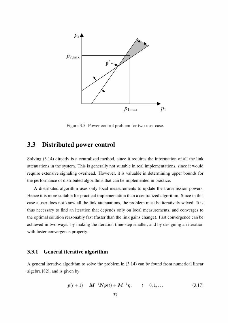
3.2.2 A two-user example . . . . . . . . . . . . . . . . . . . . . . . . . . . . 36
3.3 Distributed power control . . . . . . . . . . . . . . . . . . . . . . . . . . . . . . 37
3.3.1 General iterative algorithm . . . . . . . . . . . . . . . . . . . . . . . . . 37
3.3.2 Convergence of the iterative algorithm . . . . . . . . . . . . . . . . . . . 38
3.3.3 Convergence using standard interference functions . . . . . . . . . . . . 38
3.4 A survey of power control algorithms and state of the art . . . . . . . . . . . . . 39
3.4.1 Distributed SIR balancing algorithms . . . . . . . . . . . . . . . . . . . 39
3.4.1.1 Discrete transmission powers . . . . . . . . . . . . . . . . . . 42
3.4.2 Aiming for faster convergence . . . . . . . . . . . . . . . . . . . . . . . 42
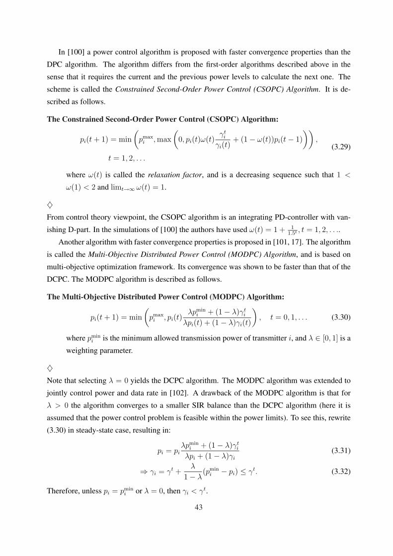
3.4.2.1 Convergence example . . . . . . . . . . . . . . . . . . . . . . 44
3.4.3 Power control for dynamical environment . . . . . . . . . . . . . . . . . 44
3.4.4 Predictive power control . . . . . . . . . . . . . . . . . . . . . . . . . . 46
3.4.5 Discussion . . . . . . . . . . . . . . . . . . . . . . . . . . . . . . . . . 47
3.5 Power control in real-time versus nonreal-time and multirate services . . . . . . . 48
3.6 Power control and other radio resource management . . . . . . . . . . . . . . . . 49
3.7 Views into the future . . . . . . . . . . . . . . . . . . . . . . . . . . . . . . . . 51
4 Adaptive closed-loop power control 534.1 Introduction . . . . . . . . . . . . . . . . . . . . . . . . . . . . . . . . . . . . . 53
4.2 Motivation for adaptive controller approach . . . . . . . . . . . . . . . . . . . . 53
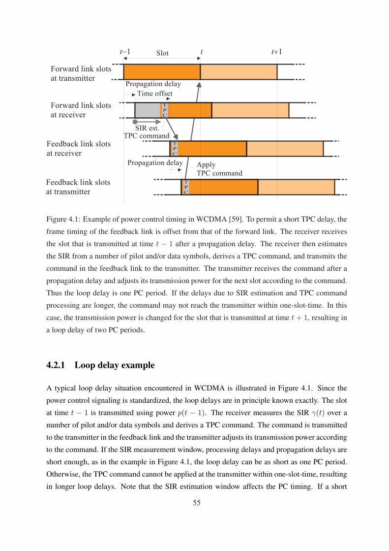
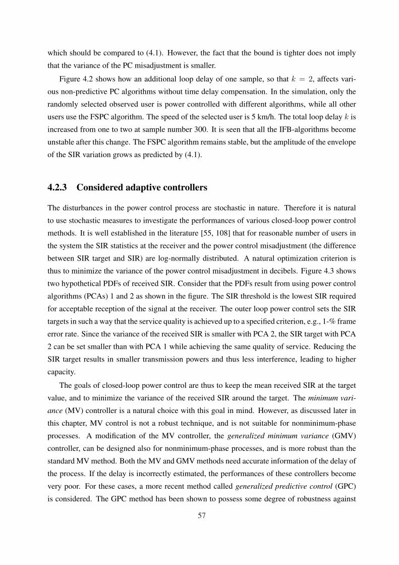
4.2.1 Loop delay example . . . . . . . . . . . . . . . . . . . . . . . . . . . . 55
4.2.2 Problems caused by the loop delay . . . . . . . . . . . . . . . . . . . . . 56
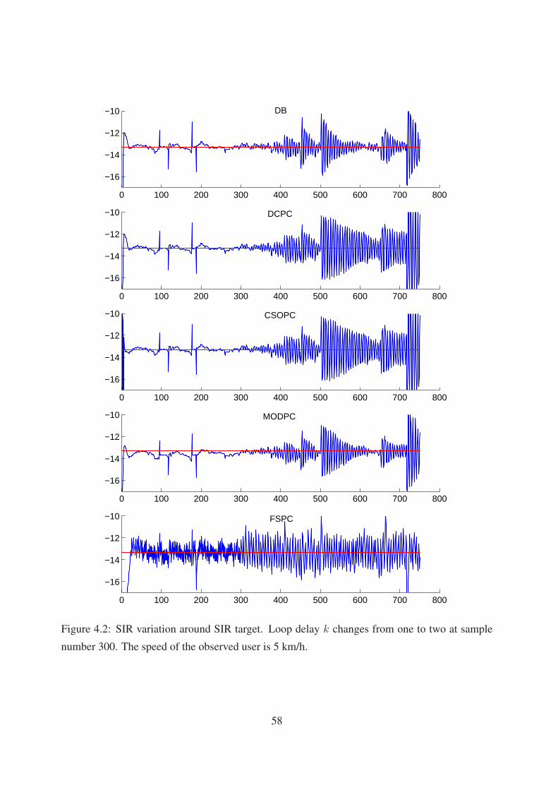
4.2.3 Considered adaptive controllers . . . . . . . . . . . . . . . . . . . . . . 57
vi
Page 9
4.2.3.1 Related work . . . . . . . . . . . . . . . . . . . . . . . . . . . 59
4.2.4 A note on the shift operator calculus used in this Chapter . . . . . . . . . 60
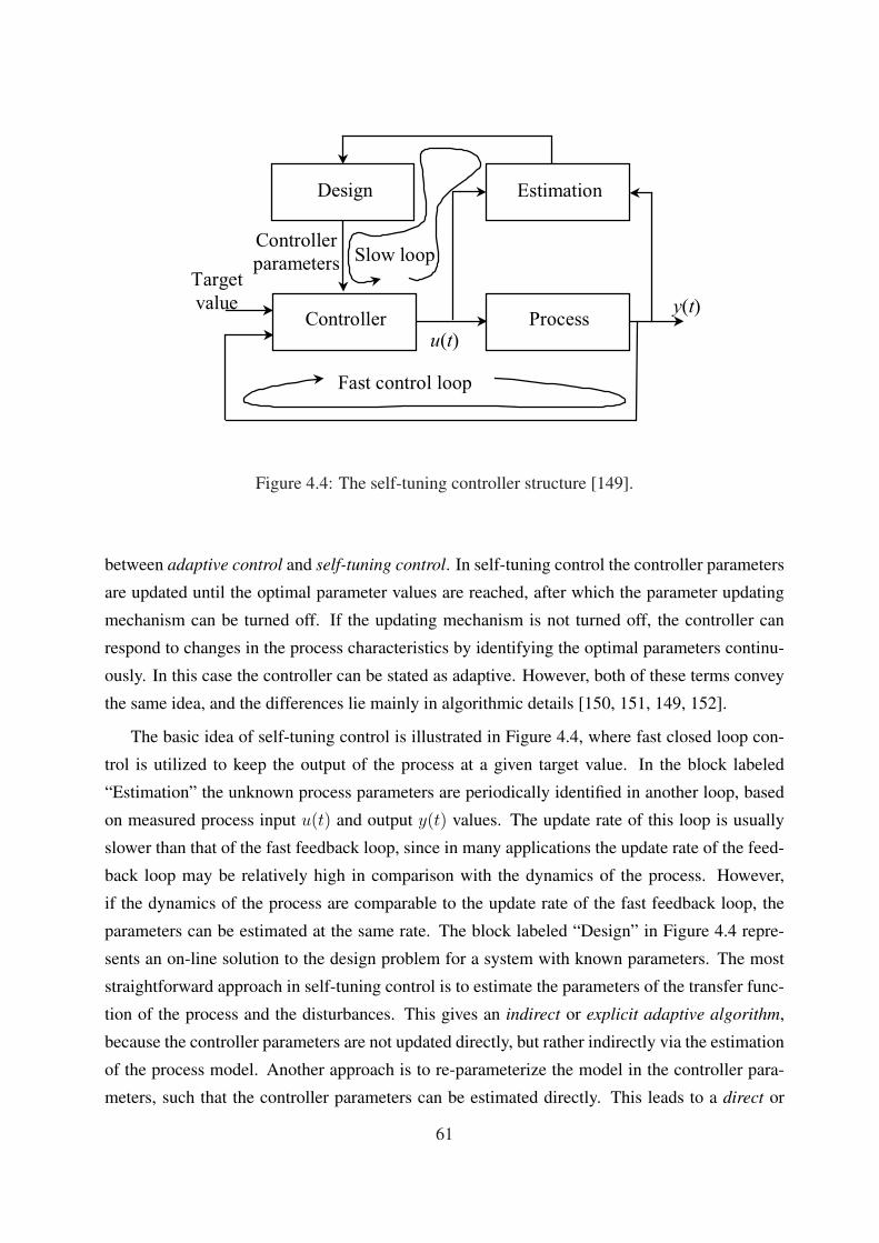
4.3 Overview of adaptive self-tuning control . . . . . . . . . . . . . . . . . . . . . . 60
4.3.1 History of adaptive control . . . . . . . . . . . . . . . . . . . . . . . . . 60
4.3.2 Characteristics of adaptive control systems . . . . . . . . . . . . . . . . 60
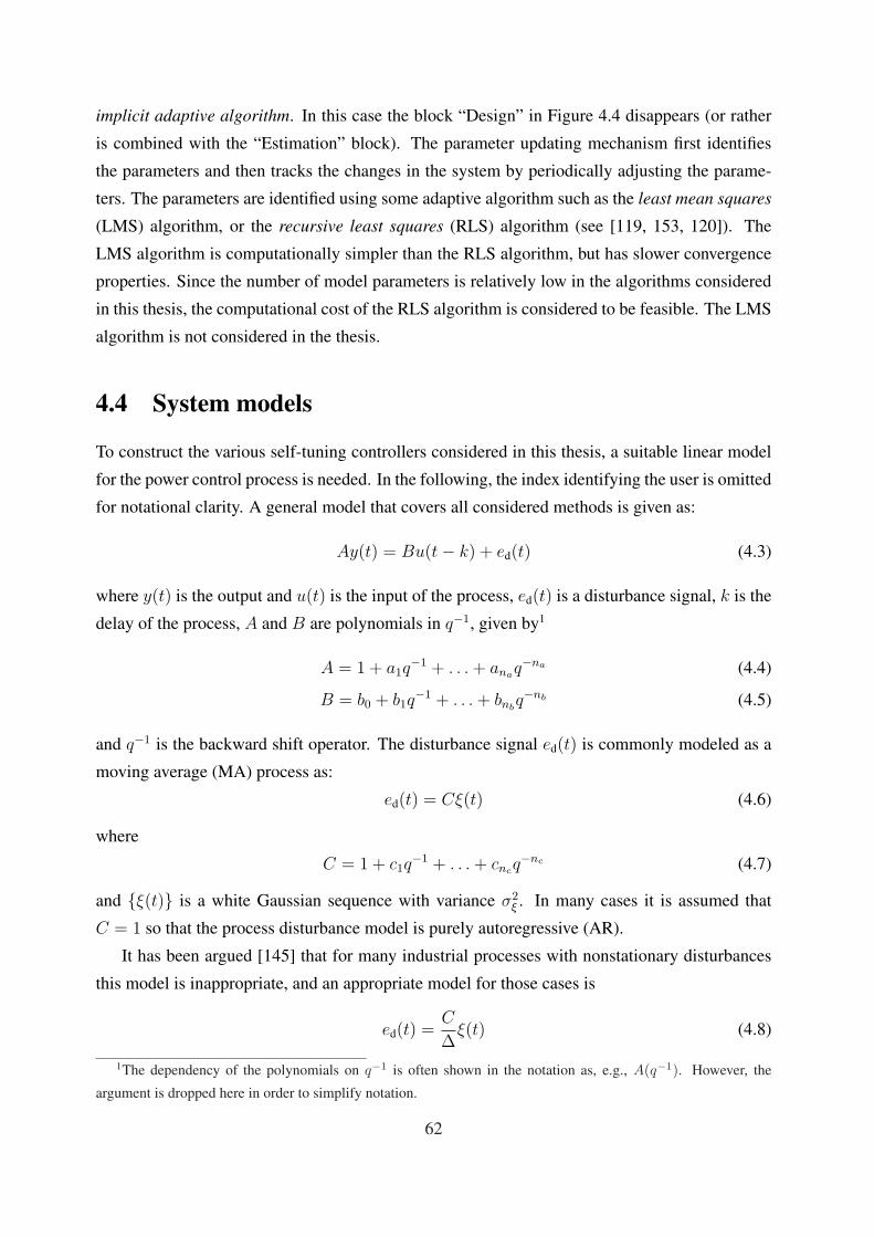
4.4 System models . . . . . . . . . . . . . . . . . . . . . . . . . . . . . . . . . . . 62
4.5 Model identification . . . . . . . . . . . . . . . . . . . . . . . . . . . . . . . . . 63
4.5.1 Data collection . . . . . . . . . . . . . . . . . . . . . . . . . . . . . . . 64
4.5.2 Model identification results . . . . . . . . . . . . . . . . . . . . . . . . 64
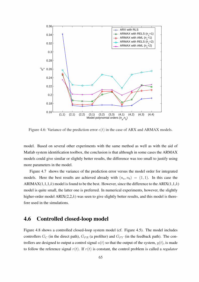
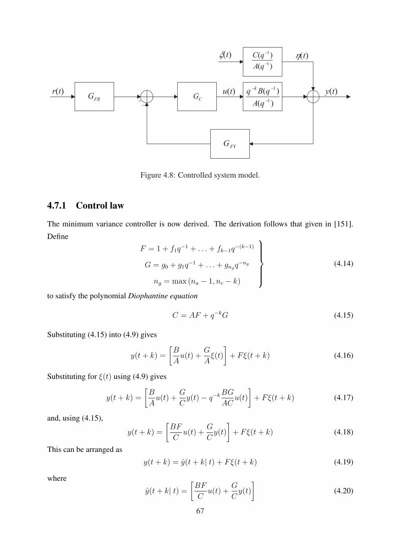
4.6 Controlled closed-loop model . . . . . . . . . . . . . . . . . . . . . . . . . . . . 65
4.7 Minimum variance (MV) control approach . . . . . . . . . . . . . . . . . . . . . 66
4.7.1 Control law . . . . . . . . . . . . . . . . . . . . . . . . . . . . . . . . . 67
4.7.2 Properties of the MV controller . . . . . . . . . . . . . . . . . . . . . . 68
4.7.3 Self-tuning minimum variance based power control algorithms . . . . . . 69
4.7.3.1 Reference signal . . . . . . . . . . . . . . . . . . . . . . . . . 69
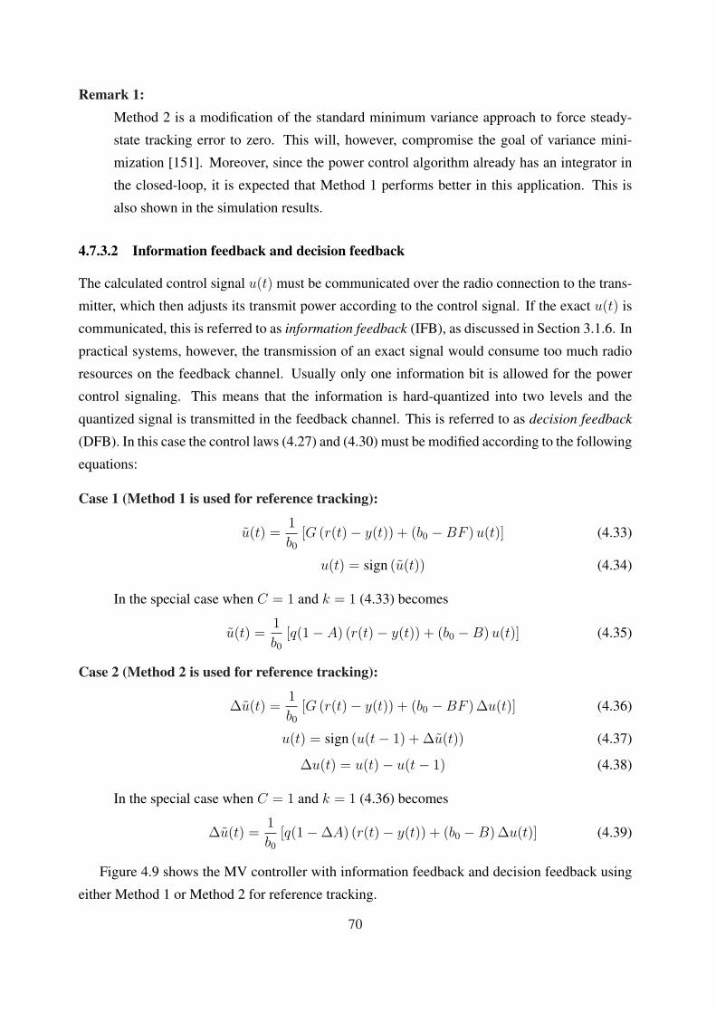
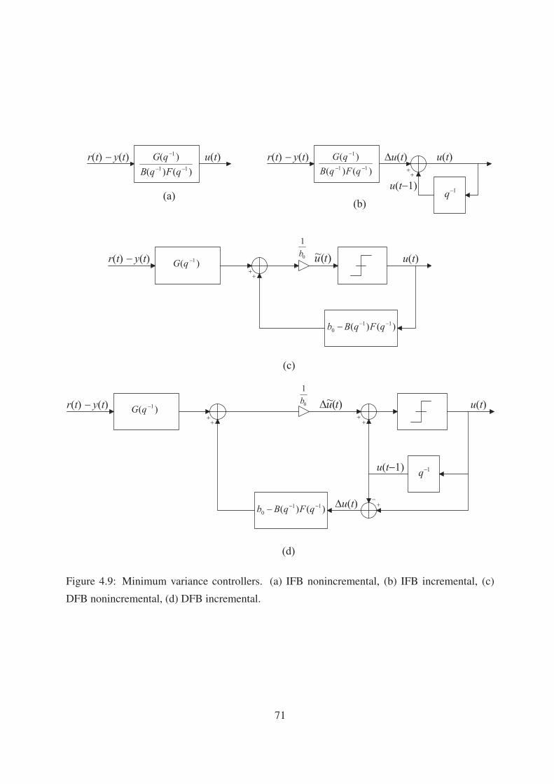
4.7.3.2 Information feedback and decision feedback . . . . . . . . . . 70
4.7.3.3 Backup controller . . . . . . . . . . . . . . . . . . . . . . . . 72
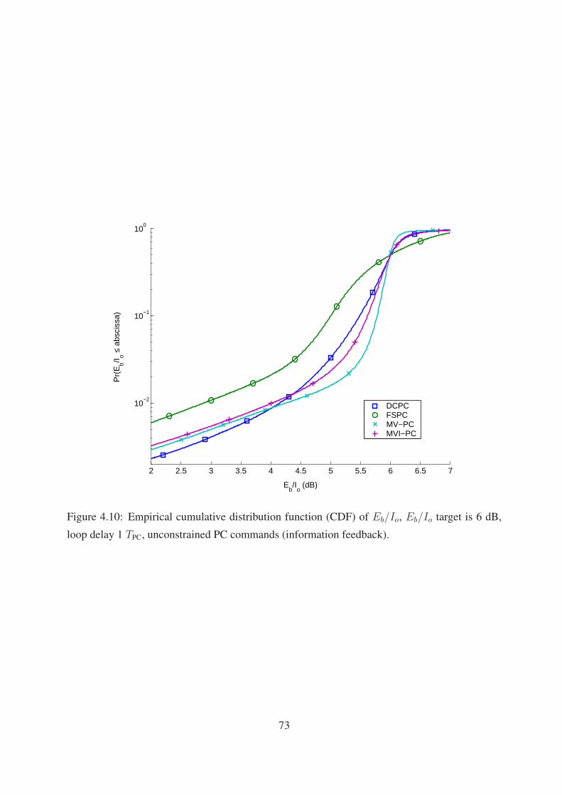
4.7.4 Simulation results . . . . . . . . . . . . . . . . . . . . . . . . . . . . . 72
4.8 Generalized minimum variance (GMV) approach . . . . . . . . . . . . . . . . . 76
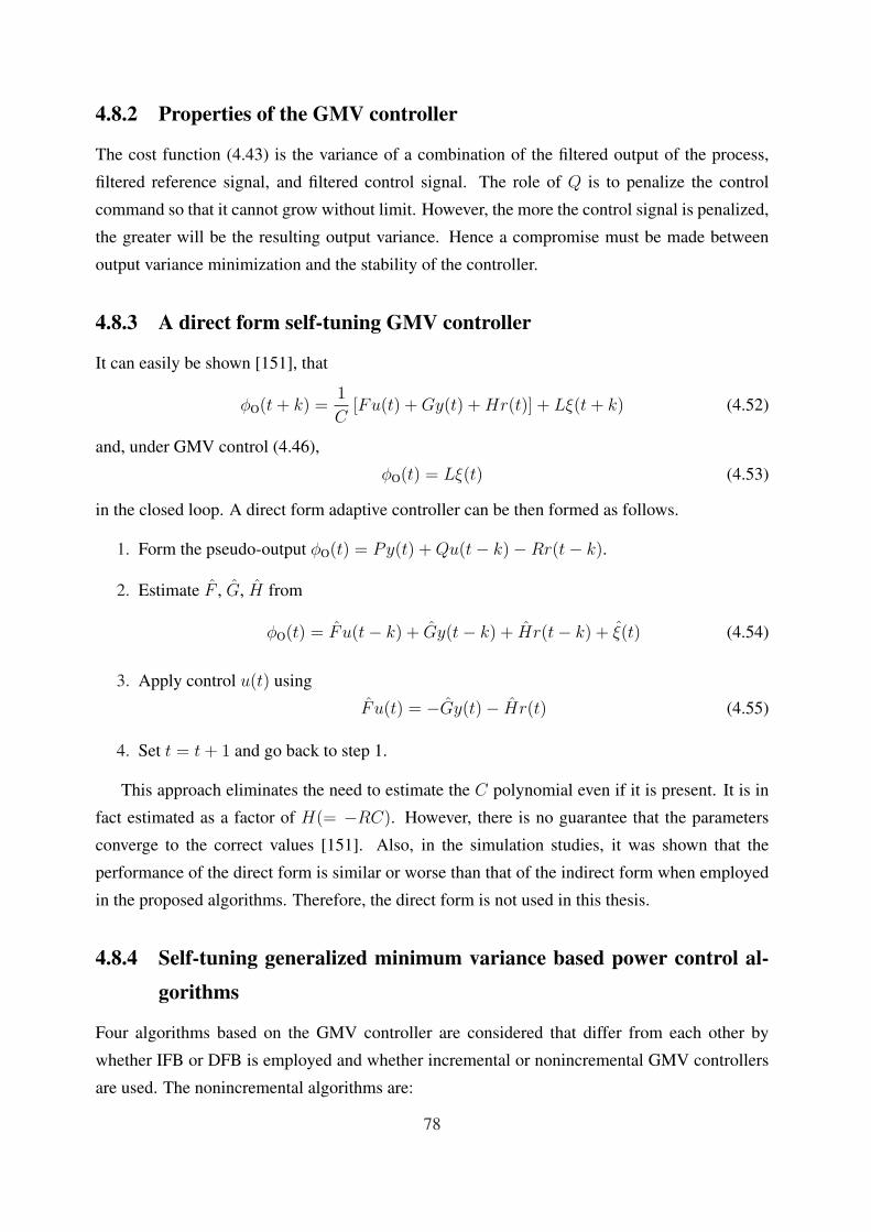
4.8.1 Control law . . . . . . . . . . . . . . . . . . . . . . . . . . . . . . . . . 77
4.8.2 Properties of the GMV controller . . . . . . . . . . . . . . . . . . . . . 78
4.8.3 A direct form self-tuning GMV controller . . . . . . . . . . . . . . . . . 78
4.8.4 Self-tuning generalized minimum variance based power control algorithms 78
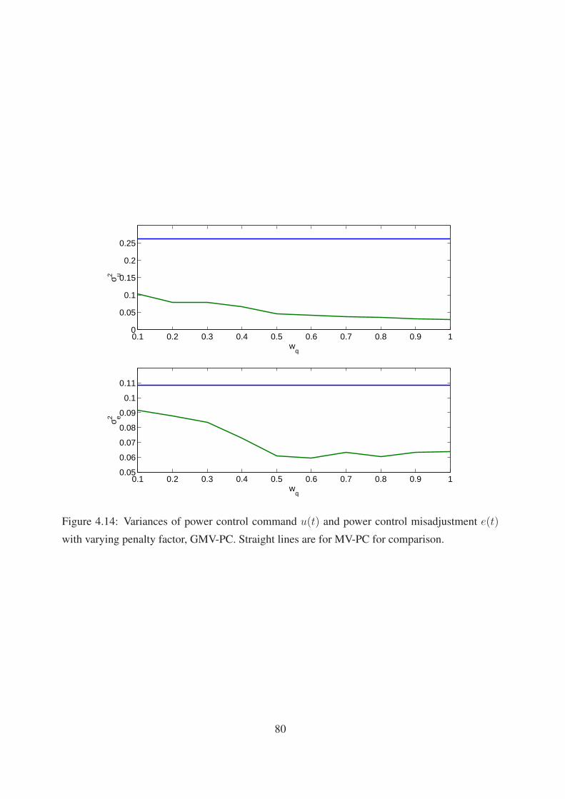
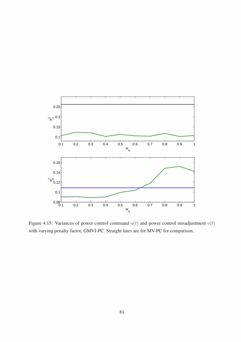
4.8.5 Simulation results . . . . . . . . . . . . . . . . . . . . . . . . . . . . . 79
4.9 Generalized predictive control (GPC) approach . . . . . . . . . . . . . . . . . . 79
4.9.1 Control law . . . . . . . . . . . . . . . . . . . . . . . . . . . . . . . . . 85
4.9.2 Properties of the GPC method . . . . . . . . . . . . . . . . . . . . . . . 87
4.9.2.1 Choice of the output and control horizons . . . . . . . . . . . 87
4.9.3 Generalized predictive control based power control algorithms . . . . . . 88
4.9.3.1 Modifications for feedback signals . . . . . . . . . . . . . . . 88
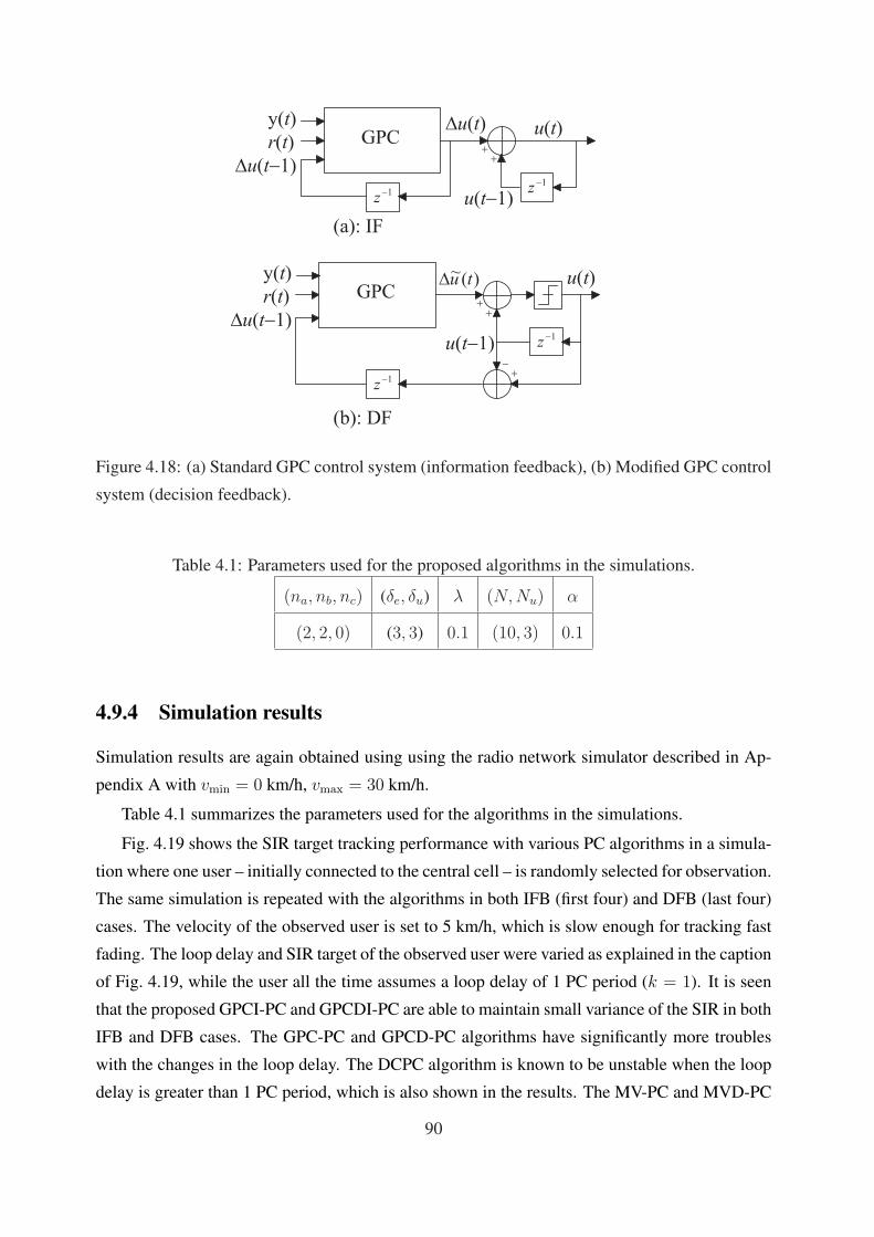
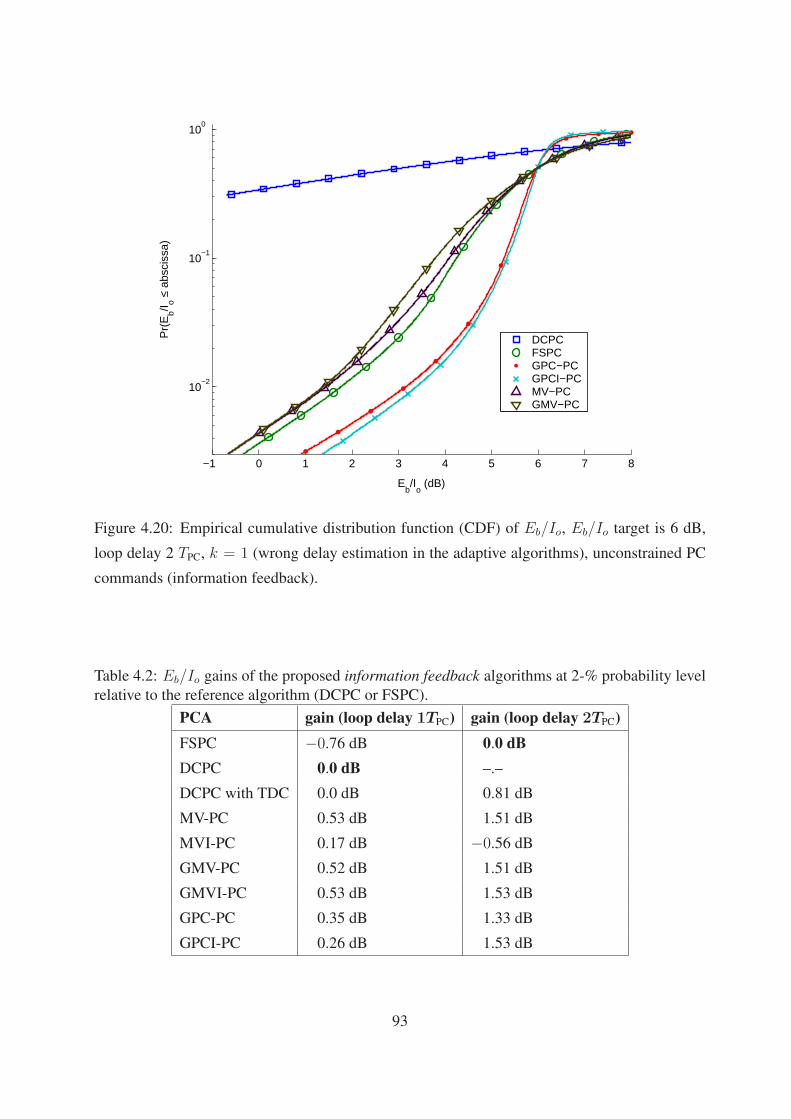
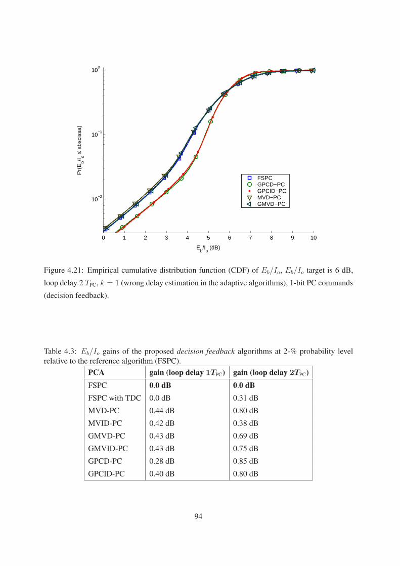
4.9.4 Simulation results . . . . . . . . . . . . . . . . . . . . . . . . . . . . . 90
4.9.4.1 About the DFB methods for GPC-based algorithms . . . . . . 91
4.10 Discussion . . . . . . . . . . . . . . . . . . . . . . . . . . . . . . . . . . . . . . 91
5 Local loop analysis 975.1 Introduction . . . . . . . . . . . . . . . . . . . . . . . . . . . . . . . . . . . . . 97
vii
Page 10
5.2 Describing Functions . . . . . . . . . . . . . . . . . . . . . . . . . . . . . . . . 97
5.3 DF Analysis of the FSPC algorithm . . . . . . . . . . . . . . . . . . . . . . . . 99
5.3.1 Example case with n = 1 . . . . . . . . . . . . . . . . . . . . . . . . . . 101
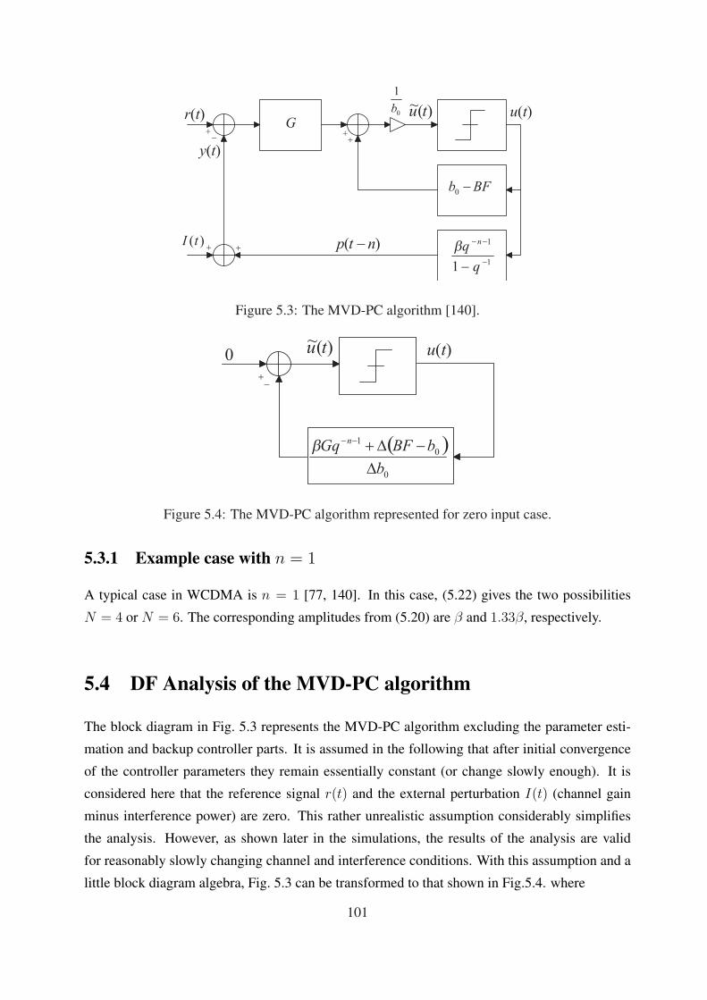
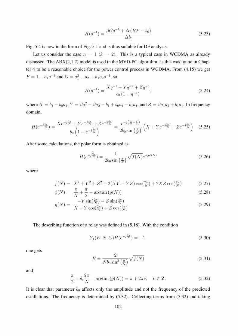
5.4 DF Analysis of the MVD-PC algorithm . . . . . . . . . . . . . . . . . . . . . . 101
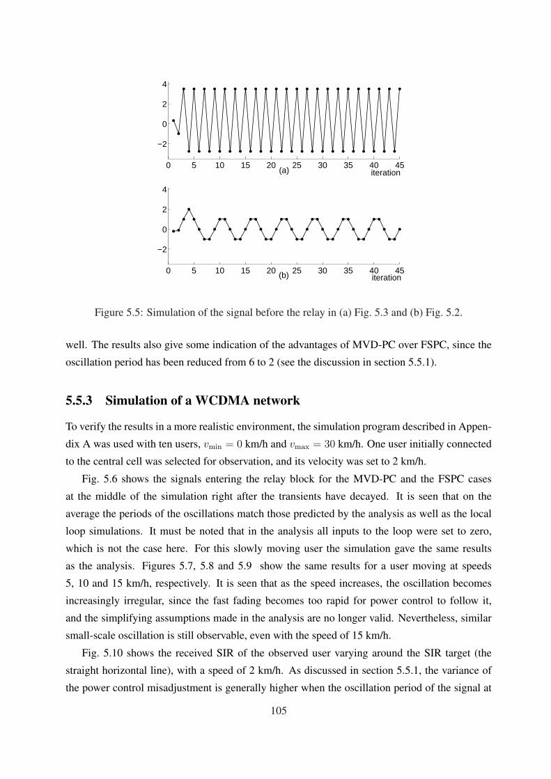
5.5 Simulation results . . . . . . . . . . . . . . . . . . . . . . . . . . . . . . . . . . 103
5.5.1 Note on the interpretation of the results . . . . . . . . . . . . . . . . . . 103
5.5.2 Simulation of the local loop . . . . . . . . . . . . . . . . . . . . . . . . 104
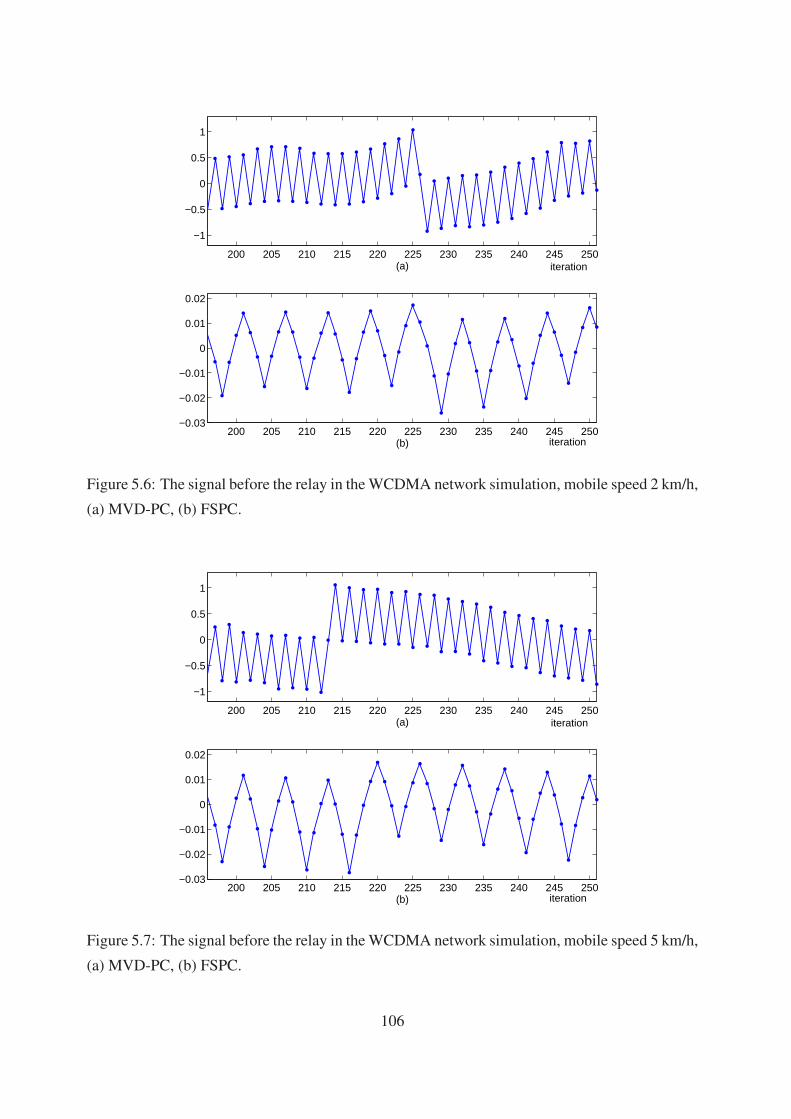
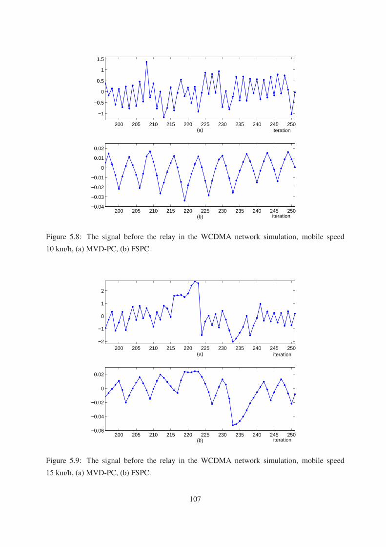
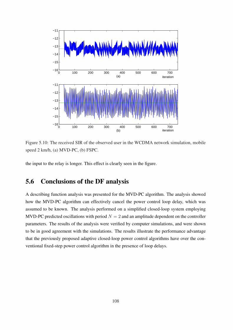
5.5.3 Simulation of a WCDMA network . . . . . . . . . . . . . . . . . . . . . 105
5.6 Conclusions of the DF analysis . . . . . . . . . . . . . . . . . . . . . . . . . . . 108
6 Adaptive step-size power control 1096.1 Introduction . . . . . . . . . . . . . . . . . . . . . . . . . . . . . . . . . . . . . 109
6.1.1 Problem setup . . . . . . . . . . . . . . . . . . . . . . . . . . . . . . . 109
6.2 Adaptation method . . . . . . . . . . . . . . . . . . . . . . . . . . . . . . . . . 110
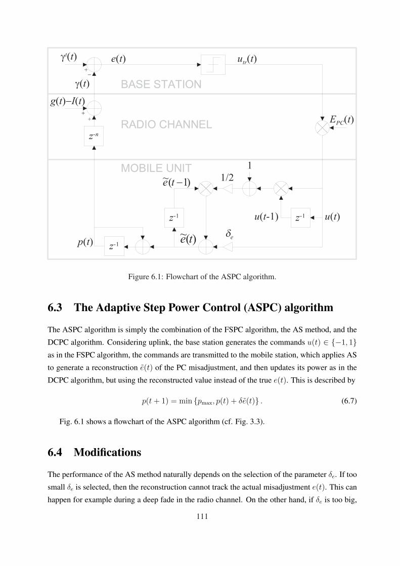
6.3 The Adaptive Step Power Control (ASPC) algorithm . . . . . . . . . . . . . . . 111
6.4 Modifications . . . . . . . . . . . . . . . . . . . . . . . . . . . . . . . . . . . . 111
6.4.1 AS with asymmetric update step sizes . . . . . . . . . . . . . . . . . . . 112
6.4.2 AS with gradually increasing update step size . . . . . . . . . . . . . . . 112
6.4.3 AS with variable update step size . . . . . . . . . . . . . . . . . . . . . 112
6.4.4 Modified ASPC algorithms . . . . . . . . . . . . . . . . . . . . . . . . . 113
6.5 Analysis on the convergence speed . . . . . . . . . . . . . . . . . . . . . . . . . 113
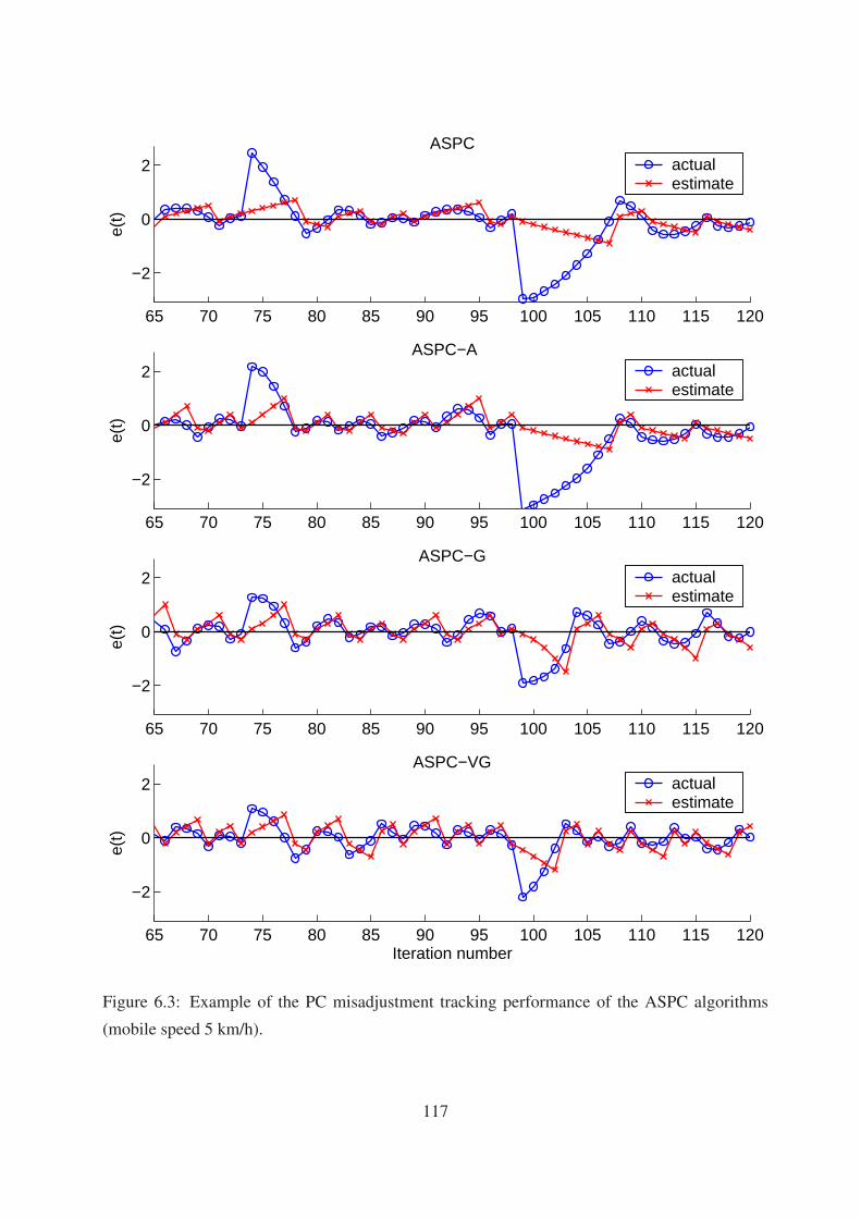
6.6 Simulation results . . . . . . . . . . . . . . . . . . . . . . . . . . . . . . . . . . 116
6.6.1 Error tracking . . . . . . . . . . . . . . . . . . . . . . . . . . . . . . . . 116
6.6.2 Convergence in two-user case . . . . . . . . . . . . . . . . . . . . . . . 118
6.6.2.1 A note on the convergence of the ASPC-VG algorithm . . . . . 119
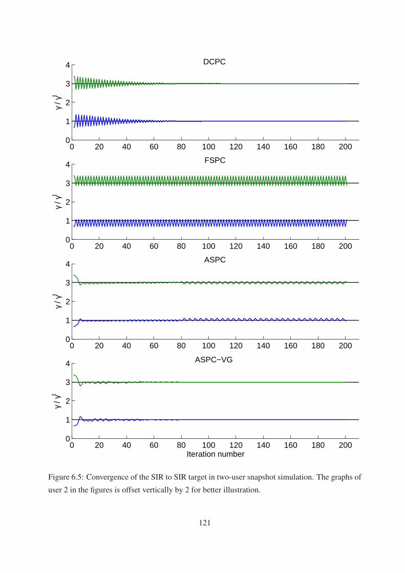
6.6.3 Performance of the ASPC algorithms . . . . . . . . . . . . . . . . . . . 123
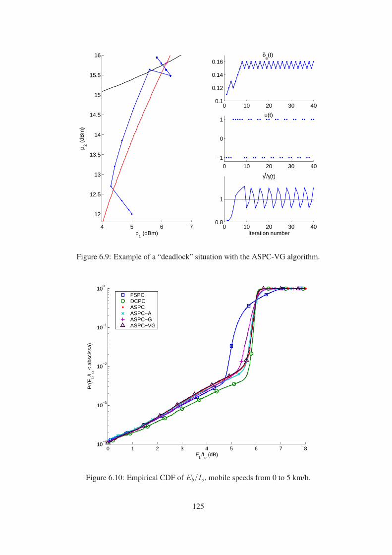
6.7 Discussion . . . . . . . . . . . . . . . . . . . . . . . . . . . . . . . . . . . . . . 127
7 Combinations and special cases 1297.1 Introduction . . . . . . . . . . . . . . . . . . . . . . . . . . . . . . . . . . . . . 129
7.2 Combining the AS method with TDC and other PC algorithms . . . . . . . . . . 129
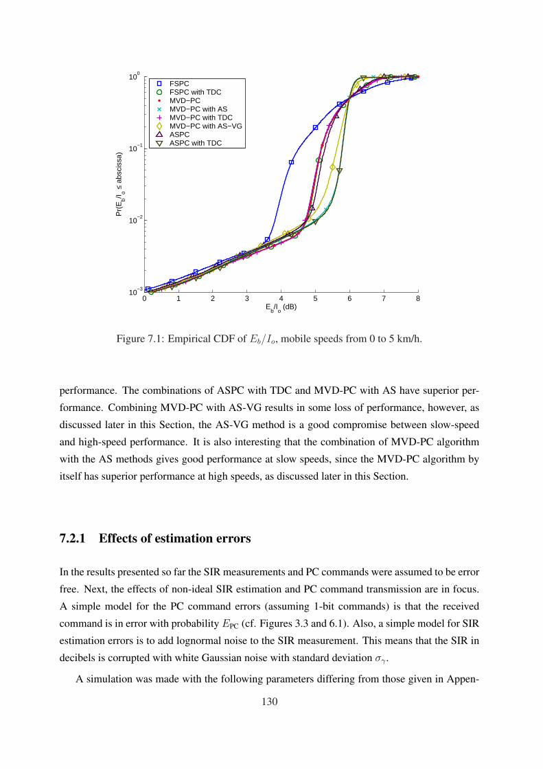
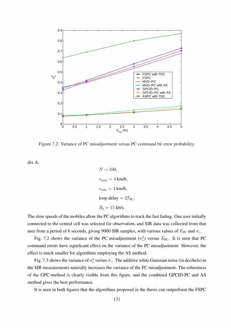
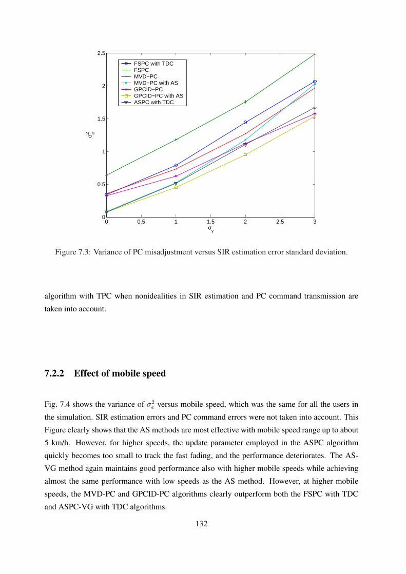
7.2.1 Effects of estimation errors . . . . . . . . . . . . . . . . . . . . . . . . . 130
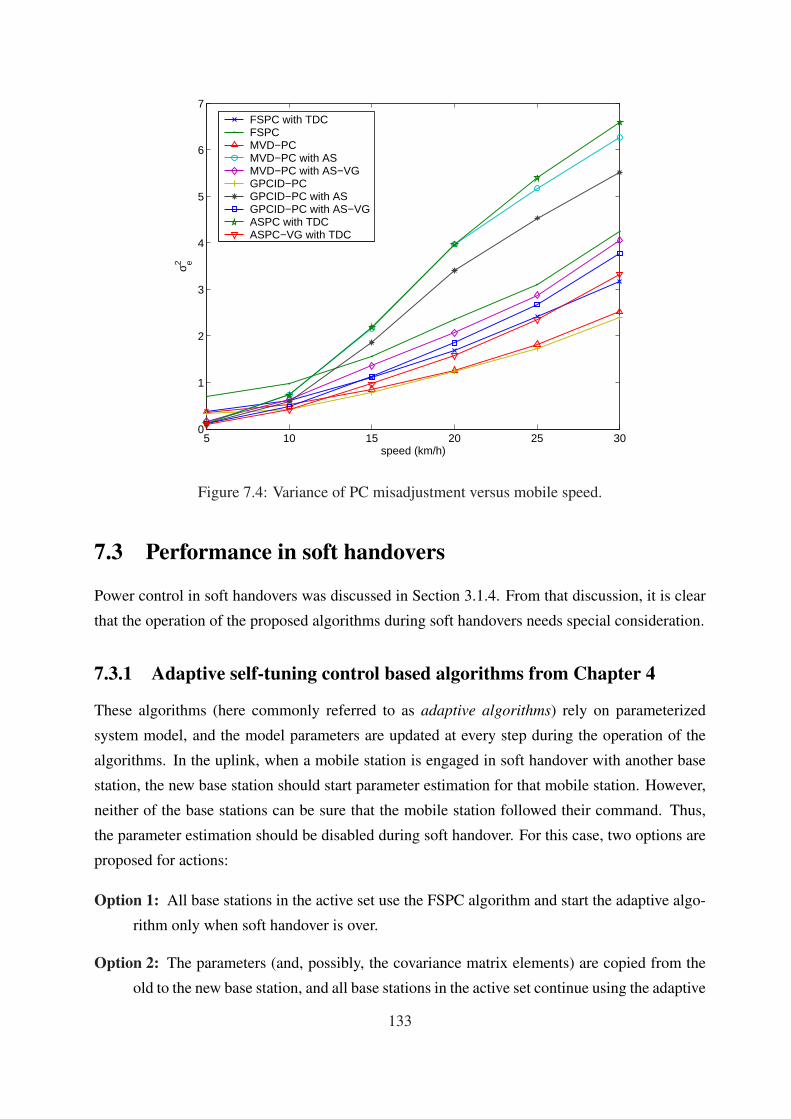
7.2.2 Effect of mobile speed . . . . . . . . . . . . . . . . . . . . . . . . . . . 132
7.3 Performance in soft handovers . . . . . . . . . . . . . . . . . . . . . . . . . . . 133
7.3.1 Adaptive self-tuning control based algorithms from Chapter 4 . . . . . . 133
7.3.2 Adaptive step-size methods of Chapter 6 . . . . . . . . . . . . . . . . . 134
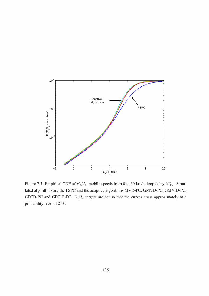
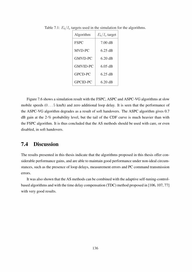
7.4 Discussion . . . . . . . . . . . . . . . . . . . . . . . . . . . . . . . . . . . . . . 136
viii
Page 11
8 Conclusions 1398.1 Open problems . . . . . . . . . . . . . . . . . . . . . . . . . . . . . . . . . . . 141
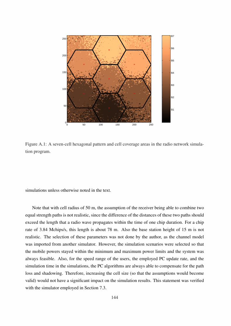
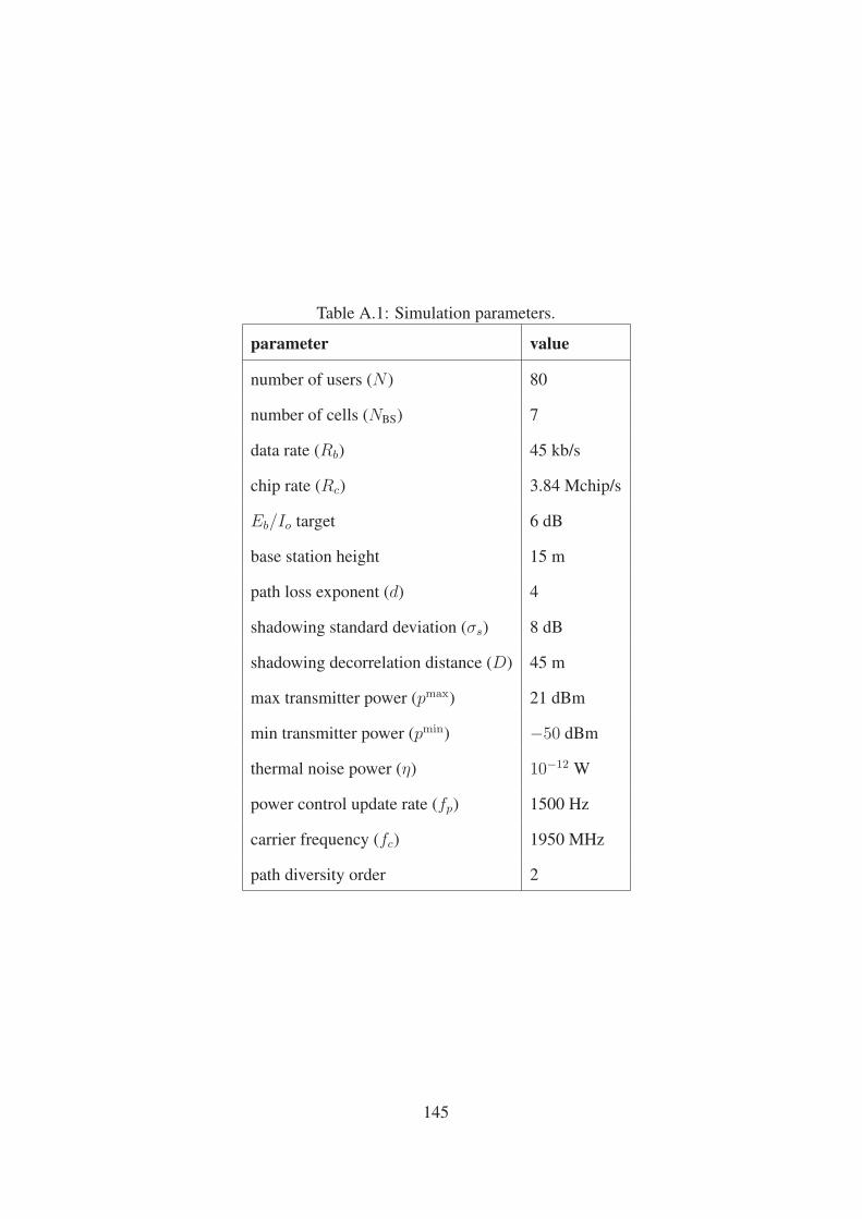
A Description of the radio network simulation program 143A.1 SIR data collection . . . . . . . . . . . . . . . . . . . . . . . . . . . . . . . . . 146
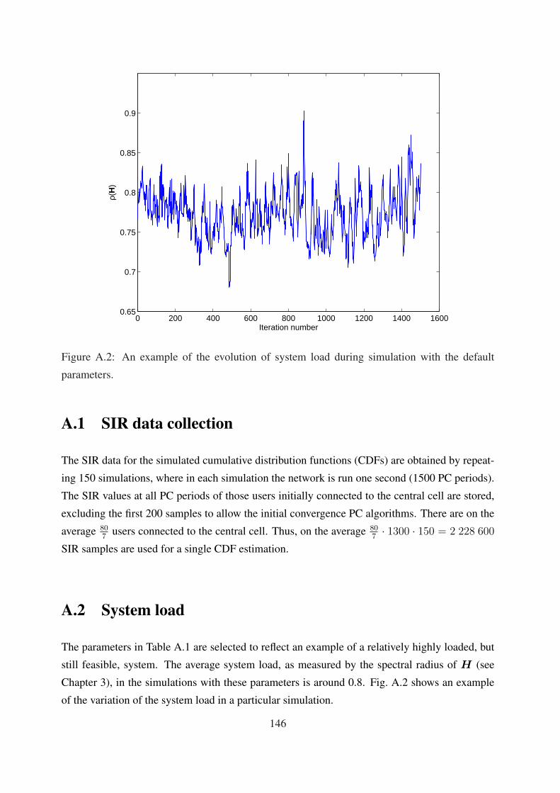
A.2 System load . . . . . . . . . . . . . . . . . . . . . . . . . . . . . . . . . . . . . 146
A.3 Reliability of the simulation results . . . . . . . . . . . . . . . . . . . . . . . . . 147
A.4 Interpretation of the results . . . . . . . . . . . . . . . . . . . . . . . . . . . . . 148
B Shift operator calculus 149
C Model identification methods 151
D The adaptive closed-loop power control algorithms proposed in Chapter 4 153D.1 Minimum variance based algorithms . . . . . . . . . . . . . . . . . . . . . . . . 153
D.1.1 MV-PC algorithm . . . . . . . . . . . . . . . . . . . . . . . . . . . . . . 153
D.1.2 MVI-PC algorithm . . . . . . . . . . . . . . . . . . . . . . . . . . . . . 153
D.1.3 MVD-PC algorithm . . . . . . . . . . . . . . . . . . . . . . . . . . . . 154
D.1.4 MVID-PC algorithm . . . . . . . . . . . . . . . . . . . . . . . . . . . . 154
D.2 Generalized minimum variance based algorithms . . . . . . . . . . . . . . . . . 154
D.2.1 GMV1-PC algorithm . . . . . . . . . . . . . . . . . . . . . . . . . . . . 154
D.2.2 GMVD-PC algorithm . . . . . . . . . . . . . . . . . . . . . . . . . . . 155
D.2.3 GMVI-PC and GMVID-PC algorithms . . . . . . . . . . . . . . . . . . 155
D.3 Generalized predictive control based algorithms . . . . . . . . . . . . . . . . . . 155
D.3.1 GPC-PC algorithm . . . . . . . . . . . . . . . . . . . . . . . . . . . . . 155
D.3.2 GPCD-PC algorithm . . . . . . . . . . . . . . . . . . . . . . . . . . . . 156
D.3.3 GPCI-PC and GPCID-PC algorithms . . . . . . . . . . . . . . . . . . . 156
Bibliography 157
ix
Page 13
List of abbreviations and symbols
Abbreviations
1G, 2G, 3G 1st, 2nd, 3rd Generation
3GPP 3rd Generation Partnership Project
3GPP2 3rd Generation Partnership Project 2
ALP Active Link Protection
AML Approximate Maximum Likelihood
AMPS Advanced Mobile Phone Service
AR Auto-Regressive Process
ARIX Auto-Regressive Integrated Process with Exogenous Input
ARIMAX Auto-Regressive Integrated Moving Average Process with Exogenous Input
ARX Auto-Regressive Process with Exogenous Input
ARMA Auto-Regressive Moving Average Process
ARMAX Auto-Regressive Moving Average Process with Exogenous Input
AS Adaptive Step
AS-A Asymmetric Adaptive Step
AS-G Gradual Adaptive Step
AS-VG Variable Gain Adaptive Step
ASPC Adaptive Step Power Control
ASPC-A Asymmetric Adaptive Step Power Control
xi
Page 14
ASPC-G Gradual Adaptive Step Power Control
ASPC-VG Variable Gain Adaptive Step Power Control
AWGN Additive White Gaussian Noise
BEP Bit Error Probability
BER Bit Error Rate
BPSK Binary Phase Shift Keying
BS Base Station
CDF Cumulative Distribution Function
CDMA Code Division Multiple Access
CDPD Cellular Digital Packet Data
CIR Carrier-to-Interference ratio
CSOPC Constrained Second-Order Power Control
DB Distributed Balancing
DCPC Distributed Constrained Power Control
DCS Digital Cellular System
DDPC Distributed Discrete Power Control
DF Describing Function
DFB Decision Feedback
DFM1, DFM2 Decision Feedback Method 1, 2
DPC Distributed Power Control
DPCCH Dedicated Physical Control Channel
DS Direct Sequence
EDGE Enhanced Data Rates for GSM Evolution
FDD Frequency Division Duplex
FDMA Frequency Division Multiple Access
xii
Page 15
FDPC Fully Distributed Power Control
FER Frame Error Rate
FH Frequency Hopping
FSPC Fixed-Step Power Control
GDCPC Generalized Distributed Constrained Power Control
GMV Generalized Minimum Variance
GMV-PC Generalized Minimum Variance Power Control
GMVD-PC Generalized Minimum Variance Decision Feedback Power Control
GMVI-PC Generalized Minimum Variance Incremental Power Control
GMVID-PC Generalized Minimum Variance Incremental Decision Feedback Power Control
GPC Generalized Predictive Control
GPC-PC Generalized Predictive Power Control
GPCD-PC Generalized Predictive Decision Feedback Power Control
GPCI-PC Generalized Predictive Incremental Power Control
GPCID-PC Generalized Predictive Incremental Decision Feedback Power Control
GPRS General Packet Radio Service
GSM Global System of Mobile Communications (originally named as Groupe Spécial
Mobile)
HSCSD High Speed Circuit Switched Data
HSD High Speed Data
HSDPA High Speed Downlink Packet Access
IFB Information Feedback
IFM1, IFM2 Information Feedback Method 1, 2
IS-xx Interim Standard - xx
IMT-2000 International Mobile Communications for the year 2000
xiii
Page 16
JTACS Japanese Total Access Communications System
LMS Least Mean Squares
LOS Line of Sight
MA Moving Average Process
M-DB Modified Distributed Balancing
MMSE Minimum-Mean-Square-Error
MODPC Multi-Objective Distributed Power Control
MOTDPC Multi-Objective Totally Distributed Power Control
MRC Maximal Ratio Combining
MS Mobile Station
MTP Minimum Transmission Power
MUD Multiuser Detection
MV Minimum Variance
MV-PC Minimum Variance Power Control
MVD-PC Minimum Variance Decision Feedback Power Control
MVI-PC Minimum Variance Incremental Power Control
MVID-PC Minimum Variance Incremental Decision Feedback Power Control
NLOS No Line of Sight
NMT Nordic Mobile Telephone
NTT The Nippon Telephone and Telegraph
ODFM Optimal Decision Feedback Method
PC Power Control
PCA Power Control Algorithm
PDC Personal Digital Cellular
PDF Probability Density Function
xiv
Page 17
PL Path loss
PRBS Pseudo-Random Binary Sequence
QoS Quality of Service
RELS Recursive Extended Least Squares
RLS Recursive Least Squares
RRM Radio Resource Management
SAS Soft and Safe Admission Control
SIR Signal-to-Interference Ratio
SMS Short Message Service
TACS Total Access Communications System
TDD Time Division Duplex
TDMA Time Division Multiple Access
TPC Transmission Power Control
UMTS Universal Mobile Telecommunication System
UTRA Universal Terrestial Radio Access
WCDMA Wideband Code Division Multiple Access
xv
Page 18
Symbols
Symbols in Chapter 1
()∗ complex conjugate
()T matrix transpose
x estimate of variable x
a correlation coefficient of shadow fading
A normalized channel attenuation matrix
Af fast fading component
Ap path loss constant
A(q−1) process model denominator polynomial
b/s bits per second
bi base station assignment variable
B(q−1) process model numerator polynomial
chip/s chips per second
C Capacity
C(q−1) noise filter numerator polynomial
d path loss exponent
Eb/Io bit-energy-to-interference-spectral-density ratio
(Eb/Io)i bit-energy-to-interference-spectral-density ratio of user i
E· expectation operator
e(t) power control misadjustment (error between measured SIR and SIR target) at
time instant t
ed(t) process disturbance at time instant t
Fn(a) estimator of a probability distribution function F (a) based on n samples
g link attenuation
xvi
Page 19
gm multipath fading power attenuation
gp path loss power attenuation
gs shadowing power attenuation
gij link attenuation between receiver i and transmitter j
g(t) link attenuation at time instant t
Gp processing gain
H normalized channel attenuation and link quality requirement matrix
I identity matrix
Io interference power spectral density
I(t) interference power in decibels at time instant t
I(p) interference function
k total loop delay
n additional loop delay (n = k − 1)
na, nb, nc, . . . order of polynomial A, B, C, . . .
N number of users
N1 minimum output horizon
N2 maximum output horizon
No noise power spectral density
Nu control horizon
pi(t) transmission power of user i at iteration t
pr received power
p normalized transmission power vector
p∗ optimal transmission power vector
Pb bit error probability
PPCE(t) probability of bit error in the power control command transmission at time instant
t
xvii
Page 20
P (t) covariance matrix at time instant t
q−1 backward time shift operator
r distance in meters
r(t) reference signal at time instant t
R source information rate
Ra(k) shadow fading correlation sequence
Rb data rate in bits/second
Rb,i data rate of user i
Rb(p) rate vector with power vector p
T sampling period
TPC power control period
u(t) process input at time instant t
urx(t) received power control command at time instant t
utx(t) transmitted power control command at time instant t
v speed
Var· Variance operator
w(t) future reference trajectory
W transmission bandwidth
x(t) regression vector at time instant t (RLS algorithm)
y(t) process output at time instant t
Yf (E, N, δe) describing function
zu u-percentile of the standard normal density function
αf forgetting factor
β PC algorithm parameter
γ Signal-to-interference ratio (SIR)
xviii
Page 21
γi SIR of user i
γi(p) SIR of user i with power vector p
γti(t) SIR target of user i at time t
γ∗ maximum achievable SIR
δ power control step size
δdown downwards step size in outer-loop PC algorithm
δe error signal threshold for switching to backup controller / power control update
parameter
δdowne power control update parameter downwards
δupe power control update parameter upwards
δup upwards step size in outer-loop PC algorithm
δVG variable gain update parameter
δu control signal threshold for switching to backup controller
δ(j) weighting sequence
∆ time difference operator
εD correlation between two points separated by distance D
ε(t) prediction error at time instant t
εE(t) prediction error at time instant t (RELS and AML algorithms)
ζ normally distributed shadowing component
ζi fraction of desired signal power that receiver i is able to utilize
η(t) additive disturbance signal of a linear process model
ηi noise power at the receiver of user i
η normalized noise power vector
θ(t) parameter vector at time instant t
θE(t) parameter vector at time instant t (RELS and AML algorithms)
xix
Page 22
λ weighting parameter
λ(j) weighting sequence
ξ(t) Gaussian distributed white noise sample at time instant t
ρ(H) spectral radius of matrix H
σ2s shadow fading variance
τp propagation delay
φ(t) residual at time instant t
φE(t) residual at time instant t (RELS and AML algorithms)
φO(t) process pseudo-output at time instant t
Φ(t) regression vector at time instant t (RELS algorithm)
Ψ(t) regression vector at time instant t (AML algorithm)
ω(t) relaxation factor
xx
Page 23
Chapter 1
Introduction
Wireless cellular communication systems have experienced a rapid growth during the last two
decades. The first-generation (1G) systems were analog and provided wireless speech service.
The major improvement in the transition to second-generation (2G) systems was the digital trans-
mission technology, which enabled the use of error correction coding and increased service qual-
ity and capacity. The 2G systems have evolved further to provide also packet-switched data
service in addition to the conventional circuit-switched services like the familiar speech service.
Today, data rates of the order of tens or even hundreds of kilobits per second are provided. Still,
the 2G systems were designed mainly for wireless speech service.
As the markets have emerged for high-speed wireless multimedia, the old speech-optimized
infrastructures are no longer enough. 2G systems, like the Global System for Mobile Commu-
nications (GSM), will continue to evolve to provide data services with data rates up to 384 kb/s.
To go beyond this, new infrastructures that are suitable for the transmission of high-speed wire-
less data are being built all over the world. These infrastructures, called third-generation (3G)
systems, are specified to provide data rates up to 2 Mb/s, which enables many new services, in-
cluding streaming video, web browsing and file transfer.1 To be of interest to the customers, the
new services should be cheap and of high quality. An important step for achieving these goals is
the selection of the multiple access method. Wideband Code Division Multiple Access (Wide-
band CDMA or WCDMA) has been selected as the air interface for these networks. The reasons
for this choice are discussed in section 1.1. The 3G system in Europe is called the Universal
Mobile Telecommunication System (UMTS) [2, 3, 4].
In CDMA systems the users transmit their signals simultaneously in the same frequency
band. Each user is given a dedicated spreading code, which is used to identify the users in the
1With the aid of High Speed Downlink Packet Access (HSDPA), even 10 Mb/s peak data rates can be supported
in hotspot areas [1]
1
Page 24
receivers by correlating the received signal with a replica of the desired user’s code.2 The cross-
correlation of different spreading codes is ideally zero, but due to multipath propagation and
non-ideal spreading codes this is not the case in practice. The receiver therefore sees the other
users’ signals as interference and the more users in the system the more interference is generated.
CDMA is interference-limited, which means that it is the interference from other users that
limits the capacity of the system. To increase capacity, some methods are needed for interference
management.
Power control (PC) aims to control the transmission powers in such a way that the co-channel
interference is minimized, while at the same time achieving sufficient quality of service (QoS).
Since in CDMA the users interfere with one another, the co-channel interference is minimized
if minimum possible transmission powers are used. The problem is then to find the minimum
transmission powers such that the QoS requirements of the users are fulfilled. Minimizing the
transmission powers has the additional desirable effect of prolonging the battery lives of the
mobile terminals. The power control problem is discussed in detail in Chapter 3.
Other means to co-channel interference management are spatial filtering and multiuser de-
tection (MUD). Spatial filtering involves the use of smart antennas (or adaptive antennas), which
consist of multi-antenna arrays with adaptive weights in the antennas. By varying the weights of
the antennas, the antenna gain towards the users can be adjusted so that the desired user’s signal
is amplified and the interfering users’ signals are attenuated. Multiuser detection takes advan-
tage of the known spreading code structure, and aims to cancel the interfering users’ signals with
known spreading codes from the received signal [5].
In this thesis the focus is on power control.
1.1 Multiple access methods
The basis for the design of the air interface in a communication system is how the common
transmission medium is shared between users, that is, the multiple access method. Different
methods have been developed to distinguish users from each other. Various aspects of different
multiple access methods are discussed, e.g., in [6, 7, 8, 9, 10].
In frequency division multiple access (FDMA), the total bandwidth of the system is divided
into narrow frequency channels using bandpass filters. These channels are then allocated to the
users. FDMA was mainly used in first generation analog cellular networks. An example of an
FDMA based system is the Nordic Mobile Telephone (NMT).
In time division multiple access (TDMA) each frequency channel is divided into time slots
2This applies to direct sequence CDMA (DS-CDMA). In frequency hopping CDMA (FH-CDMA) the code is
utilized in a different way (see section 1.1)
2
Page 25
f r e q u e n c y f r e q u e n c y f r e q u e n c y
c o d e t i m e c o d e t i m e c o d e t i m e
F D M A T D M A C D M A
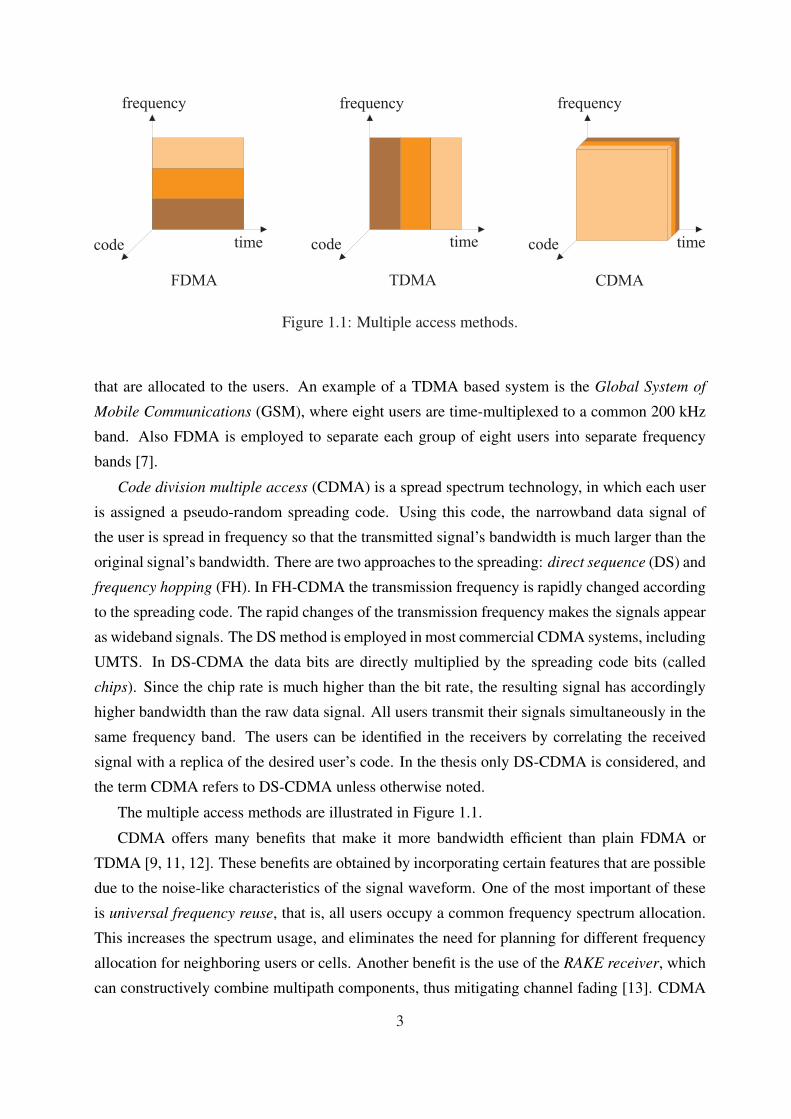
Figure 1.1: Multiple access methods.
that are allocated to the users. An example of a TDMA based system is the Global System of
Mobile Communications (GSM), where eight users are time-multiplexed to a common 200 kHz
band. Also FDMA is employed to separate each group of eight users into separate frequency
bands [7].
Code division multiple access (CDMA) is a spread spectrum technology, in which each user
is assigned a pseudo-random spreading code. Using this code, the narrowband data signal of
the user is spread in frequency so that the transmitted signal’s bandwidth is much larger than the
original signal’s bandwidth. There are two approaches to the spreading: direct sequence (DS) and
frequency hopping (FH). In FH-CDMA the transmission frequency is rapidly changed according
to the spreading code. The rapid changes of the transmission frequency makes the signals appear
as wideband signals. The DS method is employed in most commercial CDMA systems, including
UMTS. In DS-CDMA the data bits are directly multiplied by the spreading code bits (called
chips). Since the chip rate is much higher than the bit rate, the resulting signal has accordingly
higher bandwidth than the raw data signal. All users transmit their signals simultaneously in the
same frequency band. The users can be identified in the receivers by correlating the received
signal with a replica of the desired user’s code. In the thesis only DS-CDMA is considered, and
the term CDMA refers to DS-CDMA unless otherwise noted.
The multiple access methods are illustrated in Figure 1.1.
CDMA offers many benefits that make it more bandwidth efficient than plain FDMA or
TDMA [9, 11, 12]. These benefits are obtained by incorporating certain features that are possible
due to the noise-like characteristics of the signal waveform. One of the most important of these
is universal frequency reuse, that is, all users occupy a common frequency spectrum allocation.
This increases the spectrum usage, and eliminates the need for planning for different frequency
allocation for neighboring users or cells. Another benefit is the use of the RAKE receiver, which
can constructively combine multipath components, thus mitigating channel fading [13]. CDMA
3
Page 26
also enables soft handoffs among base stations, which improves cell boundary performance and
prevents dropped calls. Yet another benefit is the use of voice activity (reducing the transmission
rate during silent periods in a conversation), which reduces interference and thus has a direct
impact on capacity.
There is no single well-defined definition for wideband CDMA (WCDMA) [14]. One pro-
posed definition is based on the coherence bandwidth of the channel, i.e., the minimum distance
between two frequencies such that the channel fading at those frequencies is essentially uncor-
related. The CDMA system is called wideband CDMA if the transmission bandwidth exceeds
the coherence bandwidth. Some definitions are based on the chip rate or bandwidth as a fraction
of center frequency. Anyway, there is no distinct threshold separating narrowband CDMA from
WCDMA.
1.2 Problems and goals of this thesis
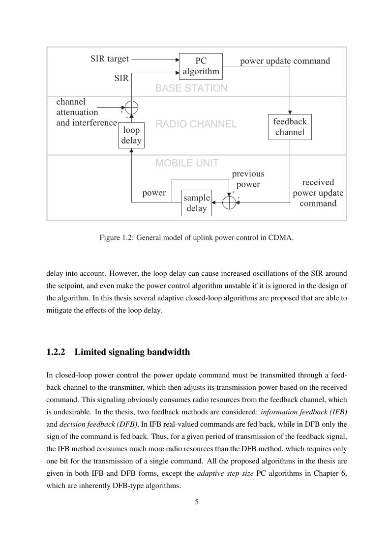
Three different power control modes can be identified in typical CDMA systems: open loop PC,
closed loop PC (or inner loop PC) and outer loop PC. Open loop PC is used in the beginning of
a radio link connection establishment to set the transmission power according to measurements
of the return channel link gain. Outer loop PC sets the target signal-to-interference ratio (SIR)
to such a level that sufficient quality of service is guaranteed, and closed loop PC aims to keep
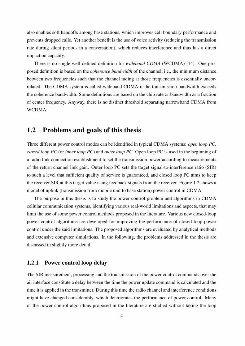
the receiver SIR at this target value using feedback signals from the receiver. Figure 1.2 shows a
model of uplink (transmission from mobile unit to base station) power control in CDMA.
The purpose in this thesis is to study the power control problem and algorithms in CDMA
cellular communication systems, identifying various real-world limitations and aspects, that may
limit the use of some power control methods proposed in the literature. Various new closed-loop
power control algorithms are developed for improving the performance of closed-loop power
control under the said limitations. The proposed algorithms are evaluated by analytical methods
and extensive computer simulations. In the following, the problems addressed in the thesis are
discussed in slightly more detail.
1.2.1 Power control loop delay
The SIR measurement, processing and the transmission of the power control commands over the
air interface constitute a delay between the time the power update command is calculated and the
time it is applied in the transmitter. During this time the radio channel and interference conditions
might have changed considerably, which deteriorates the performance of power control. Many
of the power control algorithms proposed in the literature are studied without taking the loop
4
Page 27
++
c h a n n e la t t e n u a t i o na n d i n t e r f e r e n c e
p o w e rp r e v i o u sp o w e r
p o w e r u p d a t e c o m m a n dP Ca l g o r i t h m
l o o pd e l a y
S I RS I R t a r g e t
s a m p l ed e l a y
f e e d b a c kc h a n n e l
r e c e i v e dp o w e r u p d a t ec o m m a n d+
+
Figure 1.2: General model of uplink power control in CDMA.
delay into account. However, the loop delay can cause increased oscillations of the SIR around
the setpoint, and even make the power control algorithm unstable if it is ignored in the design of
the algorithm. In this thesis several adaptive closed-loop algorithms are proposed that are able to
mitigate the effects of the loop delay.
1.2.2 Limited signaling bandwidth
In closed-loop power control the power update command must be transmitted through a feed-
back channel to the transmitter, which then adjusts its transmission power based on the received
command. This signaling obviously consumes radio resources from the feedback channel, which
is undesirable. In the thesis, two feedback methods are considered: information feedback (IFB)
and decision feedback (DFB). In IFB real-valued commands are fed back, while in DFB only the
sign of the command is fed back. Thus, for a given period of transmission of the feedback signal,
the IFB method consumes much more radio resources than the DFB method, which requires only
one bit for the transmission of a single command. All the proposed algorithms in the thesis are
given in both IFB and DFB forms, except the adaptive step-size PC algorithms in Chapter 6,
which are inherently DFB-type algorithms.
5
Page 28
1.2.3 Dynamic radio environment
A common way to study power control algorithms has been the so-called snapshot method, where
the link gains of the radio channel are assumed to be fixed, or change very slowly compared to
the dynamics of the power control algorithm. This is not very realistic, because in practice the
transmitted signals experience various kinds of fading, noise and interference. In the thesis the
main focus is on this kind of dynamical radio environment, and these dynamics are also taken
into account in the design of the proposed improved closed-loop power control algorithms.
1.2.4 Ways to achieve the goals in the thesis
In this thesis adaptive self-tuning controllers are used to reduce the undesirable effects of the loop
delay. The idea is to model the power control system from the input to the feedback channel (the
power control command) to the received SIR as a linear process and then design a controller to
make the process output, in this case the SIR at the receiver, to follow a desired reference signal,
which is the SIR target provided by the outer loop power control. An adaptation mechanism
is utilized for online identification of the model parameters. Practical versions of the proposed
algorithms are provided that achieve performance improvements without any increase in power
control signaling. Three controller approaches are considered, namely Minimum Variance (MV),
Generalized Minimum Variance (GMV) and Generalized Predictive Control (GPC). The reasons
for these choices are discussed in Chapter 4. An analytical study based on describing functions is
presented for one of the minimum-variance-based algorithms. However, due to the complexity of
the adaptation mechanisms in the proposed algorithms, their detailed analytical study becomes
prohibitively complex. Therefore, the performances of the methods are investigated using ex-
tensive computer simulations. The results are compared with well-known algorithms from the
literature. The simulations indicate that the proposed algorithms can improve the performance
of closed-loop power control significantly compared to reference algorithms in the sense that
the average SIR at a given outage probability level is higher. Outage probability is defined in
Chapter 3.
Another approach proposed in the thesis is the Adaptive Step Size (AS) method. This method
addresses the PC signaling bandwidth limitation in the DFB case, and aims at improving the
performance of DFB-type PC algorithms by adaptation of the PC step size based on the ON-
OFF PC commands. Adaptive Step Power Control (ASPC) algorithms based on the AS method
are proposed. It is shown by simulations that for slowly moving mobiles, the proposed method
improves the PC performance without violating the DFB limitation. The proposed step-size adap-
tation methods are independent from the actual power control algorithm, and can be combined
also with other power control algorithms. Examples of the combinations of the AS method and
6
Page 29
its variations with the adaptive PC algorithms proposed in Chapter 4 are given in the simulations
in Chapter 7.
While the power control methods described in this thesis can be applied to CDMA systems in
general, the main focus in this thesis is on WCDMA, and all the simulations presented are made
for WCDMA systems.
1.3 Thesis Outline
The thesis is organized as follows. After the introduction in Chapter 1, an overview on cellu-
lar radio systems is given. This chapter is mainly for those unfamiliar with such systems, and
introduces briefly the key aspects, problems and design challenges in these systems.
Power control in CDMA cellular communication systems is discussed in detail in Chapter 3,
which gives the necessary background to understand the contributions made in the thesis. A
literature survey of previous work in this area is also provided.
In Chapter 4 new adaptive closed-loop power control algorithms are proposed. The Chapter
gives an introduction to adaptive self-tuning control and recursive system identification methods,
as well as complete descriptions of the self-tuning control methods that form the basis of the
proposed algorithms. New approaches to modify the controllers for DFB are also proposed.
An analysis of the MVD-PC algorithm from Chapter 4 is provided in Chapter 5. The analysis
is based on the well-known Describing Function (DF) method. Although many simplifications
had to be made to complete the analysis, the results give valuable insight to the behavior of the
proposed algorithms.
Chapter 6 introduces the Adaptive Step (AS) method and the corresponding Adaptive Step
Power Control (ASPC) algorithm. Various modifications to improve the properties of the algo-
rithm are given, and some simulation examples demonstrating these properties are provided.
In Chapter 7 some special cases are studied, such as combinations of the AS methods of
Chapter 6 with the algorithms proposed in Chapter 4, performance in the case of measurement
errors, and performance in soft handovers.
Finally, summary and conclusions are given in Chapter 8 with comments about open issues.
1.4 Original contributions
The following original contributions are made in the thesis:
– Modeling of the closed-loop power control in WCDMA with a linear model in Chapter 4,
section 4.5.
7
Page 30
– Development of new closed-loop power control algorithms based on self-tuning controllers
and the linear model of the closed-loop power control in Chapter 4. The considered con-
trol strategies are Minimum Variance (MV) in section 4.7, Generalized Minimum Variance
(GMV) in section 4.8, and Generalized Predictive Control (GPC) in section 4.9. The al-
gorithms are capable of alleviating the undesirable effects of the loop delay inherent in the
closed-loop power control process.
– Decision feedback formulations of the considered control strategies in the case of hard-
quantized control output signals in Chapter 4, Sections 4.7, 4.8 and 4.9.
– Both information feedback (unlimited signaling bandwidth) and decision feedback (lim-
ited signaling bandwidth) versions of the proposed closed-loop power control algorithms,
where the proposed decision feedback formulations of the considered control strategies are
employed in the proposed power control algorithms.
– Describing function analysis of the MVD-PC algorithm in Chapter 5.
– The new Adaptive Step method and its modifications, as well as new PC algorithms that
are based on these methods. The ASPC algorithm was proposed in [15, 16]. The first idea
of the ASPC algorithm and the mathematics of the ASPC algorithm were contributed by
the first author in these papers. The author of this thesis refined the idea by proposing
the PC misadjustment to be reconstructed instead of SIR. All the modifications and their
related mathematics and all the simulations, including those presented in [17] are done by
the author of this thesis.
– Extensive simulations of the proposed algorithms and reference algorithms taken from the
literature.
1.5 Publications
Some of the material in the thesis has been, or will be, published elsewhere. The following is a
list of publications by the author that relate to the material in this thesis. Publication P1 is the
basis for Chapter 3. The material in Chapter 4 is for the most part covered in publications P2-P8.
The ASPC algorithm and some of its modifications are presented in publications P9-P10.
[P1] M. Rintamäki, “Power Control in CDMA Cellular Communication Systems,” in Wiley
Encyclopedia of Telecommunications, J. G. Proakis, Ed. John Wiley & Sons, 2002.
8
Page 31
[P2] I. Virtej, M. Rintamäki and H. Koivo, “Enhanced fast power control for WCDMA sys-
tems,” in Proc. IEEE Int. Symp. on Personal, Indoor and Mobile Radio Commun.
(PIMRC), London, UK, Sept. 2000, pp. 1435-1439.
[P3] M. Rintamäki, I. Virtej and H. Koivo, “Two-mode fast power control for WCDMA sys-
tems,” in Proc. IEEE Veh. Tech. Conf. (VTC), vol. 4, Rhodos, Greece, May 2001, pp.
2893-2897.
[P4] M. Rintamäki and H. Koivo, “Adaptive robust power control for WCDMA systems,” in
Proc. IEEE Veh. Tech. Conf. (VTC), vol. 1, Atlantic City, NJ, USA, Oct. 2001, pp. 62-66.
[P5] M. Rintamäki, K. Zenger and H. Koivo, “Self-tuning adaptive algorithms in the power
control of WCDMA systems,” in Proc. Nordic Signal Processing Symp. (NORSIG), boat
Hurtigruten, Norway, Oct. 2002.
[P6] M. Rintamäki, H. Koivo, and I. Hartimo, “Adaptive closed-loop power control algorithms
for CDMA cellular communication systems,” IEEE Trans. Veh. Technol., to be published.
[P7] M. Rintamäki, H. Koivo, and I. Hartimo, “Adaptive closed-loop power control algorithms
for CDMA cellular communication systems – part II,” IEEE Trans. Veh. Technol., submit-
ted for publication.
[P8] M. Rintamäki, H. Koivo, and I. Hartimo, “Application of the generalized predictive control
method in closed-loop power control of CDMA cellular communication systems,” in Proc.
Nordic Signal Processing Symp. (NORSIG), Espoo, Finland, June 2004.
[P9] M. S. Elmusrati, M. Rintamäki, I. Hartimo, and H. Koivo, “Estimated step power control
algorithm for wireless communication systems,” in Proc. Finnish Signal Processing Symp.,
Tampere, Finland, May 2003.
[P10] M. S. Elmusrati, M. Rintamäki, I. Hartimo, and H. Koivo, “Fully distributed power control
algorithm with one bit signaling and nonlinear error estimation,” in Proc. IEEE Veh. Tech.
Conf. (VTC), Orlando, FL, USA, Oct. 2003, pp. 727-731.
9
Page 33
Chapter 2
Cellular radio communication systems
This Chapter explains the basic characteristics of cellular radio communication systems. The
aim is not to give a detailed review of this enormous field, but to introduce the essential aspects
necessary to understand the problems and design challenges in such systems. The subjects that
are relevant to the thesis are presented in slightly more detail.
2.1 The development of wireless mobile communication sys-
tems
2.1.1 Historical events
The development of wireless mobile communication systems is covered in many sources, e.g.,
[18, 19, 20, 21, 7, 22, 23, 24].
The basic theory of electromagnetic fields was created by J. C. Maxwell after the middle of
the 19th century. This theory was experimentally proved by H. G. Hertz in the late 19th century.
Still before the 20th century, in 1898, the first successful use of mobile radio was done by M. G.
Marconi, who was able to establish a ship-to-shore wireless radio link over a path of 18 miles.
This event is considered to be the origin of mobile radio.
In the beginning of the 20th century, the mobile radio communication systems were used
for simple Morse-coded on-off keying-based message transmission. It was not before 1928 that
the first land mobile radio systems for broadcasting messages to police vehicles was deployed.
Since then, the mobile radio communication concept was deployed by the military, as well as
vital mobile services such as those of ambulance, fire, marine, aviation, etc. However, the quality
of the communication was poor, because at that time the technology was not mature enough to
successfully cope with the characteristics of radio wave propagation. Also, the equipment was
bulky, heavy, and consumed lots of power. Therefore, the general commercial use of mobile
11
Page 34
radio communications had to wait for the development of technology.
The mathematical foundations of information transmission were established by Shannon
[25, 26, 27]. In his work he demonstrated that the effect of a transmission power constraint,
a bandwidth constraint, and additive noise can be associated with the channel and incorporated
into a single parameter, called the channel capacity. In case of Additive White Gaussian Noise
(AWGN) channel, an ideal bandlimited channel of bandwidth W has a capacity C given by
C = W log2
(1 +
pr
WN0
)b/s, (2.1)
where pr is the average received power and N0 is the power spectral density of the additive noise.
Thus, if the source information rate R is less than C (R < C), then it is theoretically possible to
have error-free transmission of the information through the channel with appropriate coding. If
R > C, reliable transmission is not possible regardless of any signal processing at the transmitter
or receiver [13]. Shannon’s establishments gave birth to a new field called information theory.
2.1.2 The first generation (1G) cellular systems
The cellular radio concept was developed in Bell Laboratories in 1947. Instead of transmitting
signals from one location with high power, the system capacity could be dramatically increased
by limiting the range of the transmission, which enables the same frequencies to be reused at
much shorter distances. However, the concept was not implemented until 1979. It was not
until that time that the technological developments such as integrated circuits, microprocessors,
frequency synthesizers, etc., had made it possible. Soon after this came the first generation of
commercial cellular radio systems, such as The Nippon Telephone and Telegraph (NTT) system
in 1979, the Nordic Mobile Telephone (NMT) system in 1981, the Advanced Mobile Phone
Service (AMPS) in 1983 and the British Total Access Communications System (TACS) in 1985
(a modified version of AMPS). TACS is also used in Japan, where the system is called JTACS.
These systems are/were analog, and were designed for wireless speech service.
2.1.3 The second generation (2G) cellular systems
The developments of digital signal processing methods along with the rapid development of in-
tegrated circuits and microprocessors led to the replacement of the analog 1G cellular systems
by the digital 2G cellular systems. The first of these, the Global System for Mobile Communica-
tions (GSM)1, was realized in 1992 in Europe. It operates in the 900 MHz band, and is based on
1Originally GSM was an acronym for Groupe Spècial Mobile, which was the group that was established in 1982
to define the future cellular radio standards in Europe.
12
Page 35
FDMA/TDMA. Variants of GSM have been developed for higher frequency bands, such as the
Digital Cellular System 1800 (DCS 1800) in Europe and PCS 1900 in North America. The GSM
system became a huge success. As of December 2004, there were 626 GSM networks on air in
198 countries or territories around the world [28].
In North America, the AMPS system suffered from capacity limits, and it was decided that
any second-generation system must be backwards compatible with AMPS. As a result, two sys-
tems were designed and deployed: the TDMA-based D-AMPS (Digital AMPS, also known as
IS-54, and later IS-136) and the CDMA-based IS-95.
The first 2G system in Japan is called the Personal Digital Cellular (PDC) system. It is similar
to the IS-54/136 system.
The major improvements offered by the digital transmission of the 2G systems over 1G sys-
tems were better speech quality, increased capacity, global roaming, and data services like the
Short Message Service (SMS), which gained tremendous popularity in the 1990’s. Major im-
provements in the data services were also the introduction of packet switched services such as
the General Packet Radio Service (GPRS, [29, 30]), and higher-data-rate circuit switched ser-
vices such as the High Speed Circuit Switched Data service (HSCSD, [31, 32]).
2.1.4 The third generation (3G) cellular systems
Although the 2G systems could already provide some basic data services, the possible data rates
were still relatively low, and could not satisfy the needs of future mobile services like mobile web
browsing, file transfer, real-time video, digital TV, etc. The 3G cellular systems are known with
the name International Mobile Communications for the year 2000 (IMT-2000) [33], and are being
implemented in many countries around the world. The 3G systems introduce wireless wideband
packet-switched data services for wireless access to the Internet with speeds up to 2 Mb/s. The
2G systems have been (and still are) evolving towards the next generation with the introduction of
new technology enhancements, such as GPRS and HSCSD in GSM, Cellular Digital Packet Data
(CDPD, [34, 35]) that operates over AMPS, and High Speed Data (HSD, [36]) in IS-95. A step
further towards the 3G networks is the Enhanced Data rates for GSM Evolution (EDGE, [37])
technology, which enables three times higher data rates than those possible with the ordinary
GSM/GPRS network [38].
Several standardization bodies joined their forces in 1998 in the 3rd Generation Partnership
Project (3GPP) agreement [4] with the joint goal of producing globally applicable technical spec-
ifications and technical reports for a 3rd generation mobile system. It has a sister project, the 3rd
Generation Partnership Project 2 (3GPP2) [39], which comprises North American and Asian
interests developing the 3G mobile systems. The 3GPP project produces the radio interface stan-
13
Page 36
S o u r c e e n c o d e r
C h a n n e l e n c o d e r
D i g i t a l m o d u l a t o r
C h a n n e l
S o u r c e d e c o d e r
C h a n n e l d e c o d e r
D i g i t a l D e m o d u l a t o r
M e s s a g e
E s t i m a t e o f m e s s a g e
T r a n s m i t t e r
R e c e i v e r
Figure 2.1: A digital communication link.
dard for the 3G networks, wideband CDMA (WCDMA), which is the main 3rd generation air
interface in the world and will be deployed in Europe and Asia, including Japan and Korea.
The 3G systems within the scope of 3GPP are generally known with the name Universal Mo-
bile Telecommunication Services (UMTS), and WCDMA is called Universal Terrestrial Radio
Access (UTRA) Frequency Division Duplex (FDD) and Time Division Duplex (TDD), the name
WCDMA being used to cover both FDD and TDD operation [3].
The air interface to be developed by 3GPP2 is referred to as cdma2000, which is based partly
on IS-95 principles. It is further divided to two standards, namely cdma2000 1x and cdma2000
3x. cdma2000 1x is considered a 2.5G system, and it has the same bandwidth (1.25 MHz) as
IS-95. cdma2000 3x is the 3G variant of cdma2000. It is a wideband version with three times
the bandwidth of IS-95 [40].
2.2 Wireless digital radio communication
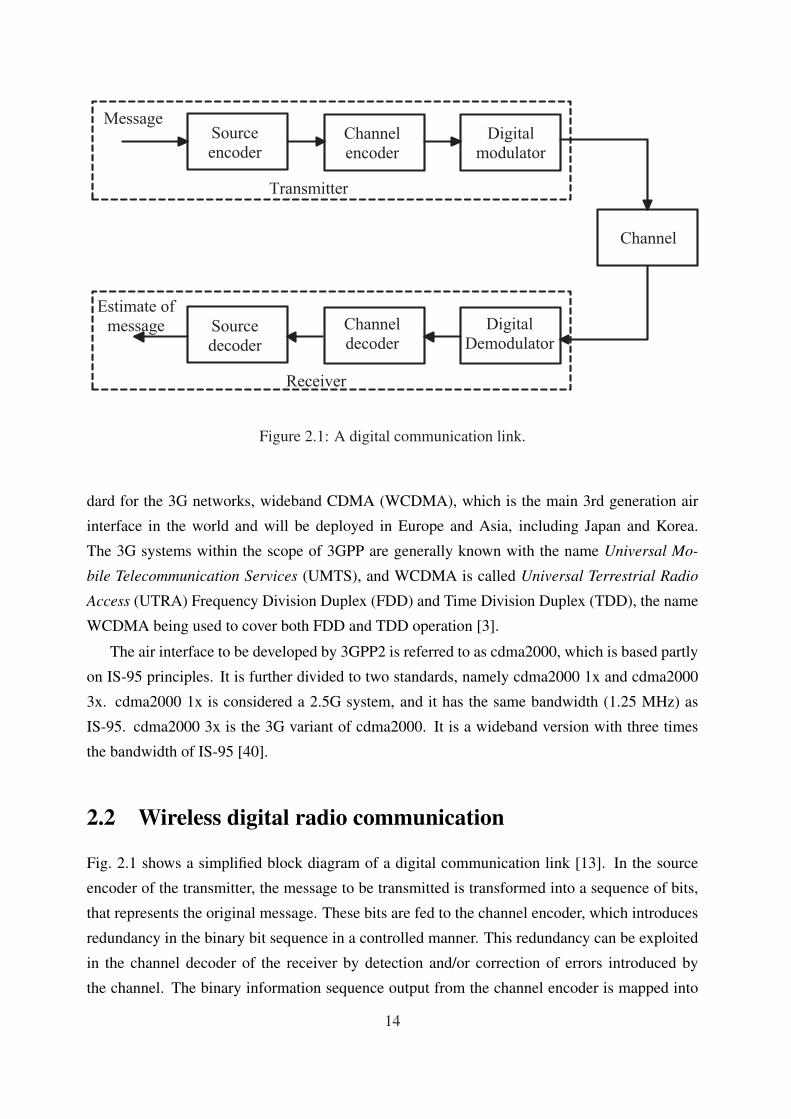
Fig. 2.1 shows a simplified block diagram of a digital communication link [13]. In the source
encoder of the transmitter, the message to be transmitted is transformed into a sequence of bits,
that represents the original message. These bits are fed to the channel encoder, which introduces
redundancy in the binary bit sequence in a controlled manner. This redundancy can be exploited
in the channel decoder of the receiver by detection and/or correction of errors introduced by
the channel. The binary information sequence output from the channel encoder is mapped into
14
Page 37
signal waveforms in the digital modulator, and fed to the channel. In the case of wireless radio
communication, the waveforms are transmitted as electromagnetic waves through transmission
antenna(s).
The channel introduces various forms of corruption to the transmitted signal, like noise, in-
terference from other transmitters, and fading (fluctuations in the channel gain). The task of the
receiver is to capture the transmitted signal, and remove the effects of the channel as well as the
processing in the transmitter. Firstly, the demodulator converts the received waveforms into a
binary sequence, which is fed to the channel decoder. The channel decoder removes the redun-
dancy introduced by the channel encoder in the transmitter, and attempts to detect and/or correct
possible bit errors using the knowledge of the code used by the channel encoder and the redun-
dancy contained in the received data. The frequency at which bit errors occur at the output of the
channel decoder is a measure of the demodulator-decoder performance. Typically the Bit Error
Rate (BER) at this point is kept at a desired level so as to have acceptable quality of communi-
cation with minimum resource usage. Finally, the source decoder tries to reconstruct the original
message from the decoded binary sequence. This will be an estimation of the original message
due to the possible corruption introduced to the data along its way through the communication
link.
2.2.1 Properties of a radio communications channel
A radio communications link includes everything from the information source, through all the
encoding and modulation steps, through the transmitter and channel, up to and including the
receiver and all its signal processing steps, as well as the information sink [41]. The term channel
can be defined in many ways, depending on the context that it is used in. Generally one can view
a channel as the link between two points along a path of communications [7]. For example, a
digital channel is the link between the input to the modulator and the output of the demodulator
(see Fig. 2.1), while a radio propagation channel is the physical medium in which the radio
waves propagate from the transmitter antenna to the receiver antenna. A radio channel is the
combination of the transmitter and receiver antennas and the radio propagation channel. Radio
channel is comprehensively discussed in, e.g., [41, 7, 10, 21]. The discussion here is limited to
the radio channel.
The attenuation of a radio signal can be modeled as a product of three effects, namely path
loss (gp), shadowing (gs) and multipath fading (gm) [18, 19] as
g = gpgsgm. (2.2)
Path loss is the large-scale distance-dependent attenuation in the average signal power. Shad-
owing is the medium-scale attenuation, which is caused by diffraction and shielding phenomena
15
Page 38
caused by terrain variations. Multipath fading is the rapid fluctuation in the received signal power
that is caused by the constructive and destructive addition of the signals that propagate through
different paths with different delays from the transmitter to the receiver. These effects are ex-
plained in more detail in the following.
2.2.1.1 Path loss
Path loss is the large-scale distance-dependent attenuation in the average signal power. Early
studies by Okumura [42] and Hata [43] yielded path loss models for urban, suburban and rural
areas. Based on their ideas, a widely accepted model for path loss (or path gain) gp is described
as
gp =Ap
rd, (2.3)
where Ap is a constant depending on the antenna properties, transmission wavelength, and the
environment (rural, suburban, urban), r is the distance between the transmitter and receiver in
meters at time t and d is the path loss exponent with typical values ranging from 2 (free space
propagation) to 5 (dense urban areas).
2.2.1.2 Shadowing
Shadowing, also known as slow fading, is the medium-scale attenuation, which is caused by dif-
fraction and shielding phenomena caused by terrain variations. This results in relatively slow
variations in the mean signal power over a distance of a few tens of wavelengths. It is caused by
reflections, refractions and diffractions of the signal from buildings, trees, rocks, etc. It is com-
monly modeled as a log-normally distributed random variable with zero dB mean and a standard
deviation of typically 3 to 10 dB. A simple model for the spatial correlation of shadowing was
proposed in [44]. In this model, the shadowing is a log-normally distributed random variable with
an exponential correlation function. The correlation function was fitted to experimental data from
a 900 MHz measurement in suburban environment and from a 1700 MHz measurement in urban
areas. Formally, the shadowing correlation is given by
Ra(k) = σ2sa|k|, (2.4)
a = εvT/DD , (2.5)
where σ2s is the variance of the shadowing, a is the correlation coefficient, εD is the correlation
between two points separated by distance D, v is the speed of the mobile station moving in the
terrain, and T is the sampling period. This model can be easily implemented by filtering a white
Gaussian noise process through a first-order filter with a pole at a.
16
Page 39
2.2.1.3 Multipath fading
Multipath fading, or fast fading, is the rapid fluctuation in the received signal power that is caused
by the constructive and destructive addition of the signals that propagate through different paths
with different delays from the transmitter to the receiver. In urban environment the number of
significant signal paths is typically much larger than in rural areas. This affects the multipath
spread, which is the roughly the time between the first occurrence of the transmitted signal at
the receiver and the last significant reflection of the same signal at the receiver. If the multipath
spread is longer than the inverse of the bandwidth of the information-bearing signal, i.e., longer
than the duration of a transmitted symbol, then the fading is said to be frequency-selective. Oth-
erwise it is frequency-non-selective, or flat. In spread-spectrum systems, typically, the fading is
frequency-selective, and this can be exploited with the use of a RAKE receiver, which coherently
combines the signals received from different paths.
The multipath fading is usually modeled as a filtered complex Gaussian process, resulting
in a Rayleigh-distributed envelope, and a classical Doppler spectrum. This model is applicable
in no-line-of-sight (NLOS) situations. If a line-of-sight (LOS) signal is present, then the fading
envelope can be modeled with a Rice distribution. Also Nakagami distribution has been widely
used to model multipath fading [21]. Jakes [18] proposed a model for a Rayleigh fading simulator
with the required spectral properties based on a sum of sinusoids. This model is still widely used.
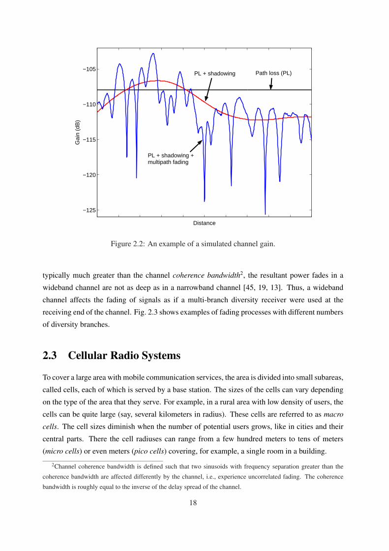
2.2.1.4 Example: simulated channel gain
All the above three effects included, the power gain g of the channel in linear scale can be
modeled as:
g = gpgsgm = Apr−d10
ζ10 Af (2.6)
where ζ is a Gaussian random variable with zero mean, standard deviation between 3 to 10, and
exponential correlation function. Af is a random variable such that√
Af is either Rayleigh-,
Rice- or Nakagami distributed with a classical Doppler spectrum. An example of a simulated
channel gain is shown in Fig. 2.2.
2.2.1.5 Wideband radio transmission
In spread spectrum systems such as DS-CDMA the transmission bandwidth is much greater than
what is needed to represent the information signal. Wideband transmission has some appealing
features over narrowband transmission. Since the transmission bandwidth in such systems is
17
Page 40
−125
−120
−115
−110
−105
Distance
Gai
n (d
B)
PL + shadowing Path loss (PL)
PL + shadowing +multipath fading
Figure 2.2: An example of a simulated channel gain.
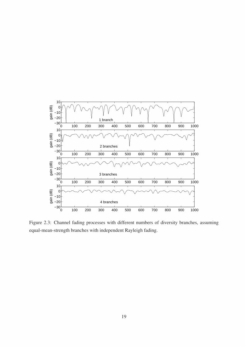
typically much greater than the channel coherence bandwidth2, the resultant power fades in a
wideband channel are not as deep as in a narrowband channel [45, 19, 13]. Thus, a wideband
channel affects the fading of signals as if a multi-branch diversity receiver were used at the
receiving end of the channel. Fig. 2.3 shows examples of fading processes with different numbers
of diversity branches.
2.3 Cellular Radio Systems
To cover a large area with mobile communication services, the area is divided into small subareas,
called cells, each of which is served by a base station. The sizes of the cells can vary depending
on the type of the area that they serve. For example, in a rural area with low density of users, the
cells can be quite large (say, several kilometers in radius). These cells are referred to as macro
cells. The cell sizes diminish when the number of potential users grows, like in cities and their
central parts. There the cell radiuses can range from a few hundred meters to tens of meters
(micro cells) or even meters (pico cells) covering, for example, a single room in a building.
2Channel coherence bandwidth is defined such that two sinusoids with frequency separation greater than the
coherence bandwidth are affected differently by the channel, i.e., experience uncorrelated fading. The coherence
bandwidth is roughly equal to the inverse of the delay spread of the channel.
18
Page 41
0 100 200 300 400 500 600 700 800 900 1000−30
−20
−10
0
10
1 branchgain
(dB
)
0 100 200 300 400 500 600 700 800 900 1000−30
−20
−10
0
10
2 branchesgain
(dB
)
0 100 200 300 400 500 600 700 800 900 1000−30
−20
−10
0
10
3 branchesgain
(dB
)
0 100 200 300 400 500 600 700 800 900 1000−30
−20
−10
0
10
4 branchesgain
(dB
)
Figure 2.3: Channel fading processes with different numbers of diversity branches, assuming
equal-mean-strength branches with independent Rayleigh fading.
19
Page 42
0 50 100 150 200 2500
50
100
150
200
250
B1
B2
B3
B4
B5
B6
B7
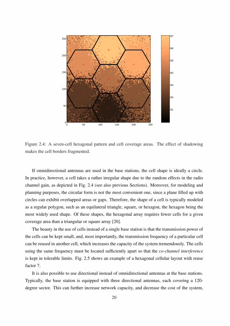
Figure 2.4: A seven-cell hexagonal pattern and cell coverage areas. The effect of shadowing
makes the cell borders fragmented.
If omnidirectional antennas are used in the base stations, the cell shape is ideally a circle.
In practice, however, a cell takes a rather irregular shape due to the random effects in the radio
channel gain, as depicted in Fig. 2.4 (see also previous Sections). Moreover, for modeling and
planning purposes, the circular form is not the most convenient one, since a plane filled up with
circles can exhibit overlapped areas or gaps. Therefore, the shape of a cell is typically modeled
as a regular polygon, such as an equilateral triangle, square, or hexagon, the hexagon being the
most widely used shape. Of these shapes, the hexagonal array requires fewer cells for a given
coverage area than a triangular or square array [20].
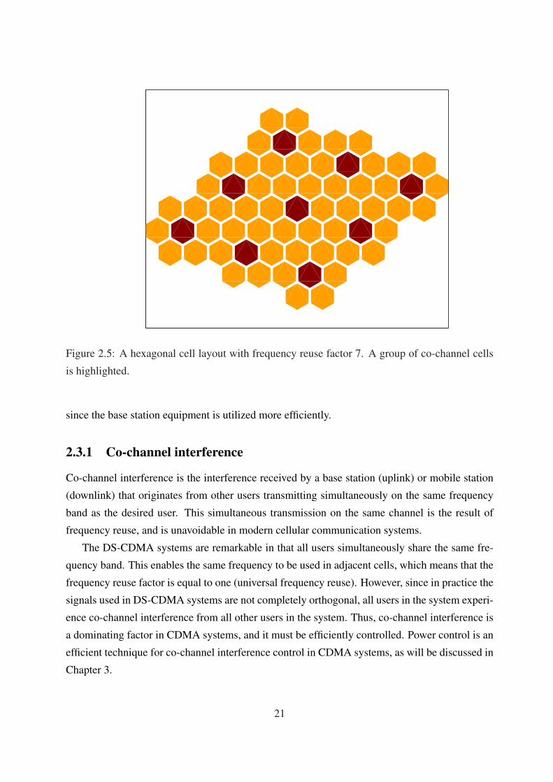
The beauty in the use of cells instead of a single base station is that the transmission power of
the cells can be kept small, and, most importantly, the transmission frequency of a particular cell
can be reused in another cell, which increases the capacity of the system tremendously. The cells
using the same frequency must be located sufficiently apart so that the co-channel interference
is kept in tolerable limits. Fig. 2.5 shows an example of a hexagonal cellular layout with reuse
factor 7.
It is also possible to use directional instead of omnidirectional antennas at the base stations.
Typically, the base station is equipped with three directional antennas, each covering a 120-
degree sector. This can further increase network capacity, and decrease the cost of the system,
20
Page 43
Figure 2.5: A hexagonal cell layout with frequency reuse factor 7. A group of co-channel cells
is highlighted.
since the base station equipment is utilized more efficiently.
2.3.1 Co-channel interference
Co-channel interference is the interference received by a base station (uplink) or mobile station
(downlink) that originates from other users transmitting simultaneously on the same frequency
band as the desired user. This simultaneous transmission on the same channel is the result of
frequency reuse, and is unavoidable in modern cellular communication systems.
The DS-CDMA systems are remarkable in that all users simultaneously share the same fre-
quency band. This enables the same frequency to be used in adjacent cells, which means that the
frequency reuse factor is equal to one (universal frequency reuse). However, since in practice the
signals used in DS-CDMA systems are not completely orthogonal, all users in the system experi-
ence co-channel interference from all other users in the system. Thus, co-channel interference is
a dominating factor in CDMA systems, and it must be efficiently controlled. Power control is an
efficient technique for co-channel interference control in CDMA systems, as will be discussed in
Chapter 3.
21
Page 45
Chapter 3
Power control in CDMA cellularcommunication systems
The aim in this Chapter is to give a somewhat detailed overview of power control in CDMA
cellular communication systems and to present the relevant problems within the scope of the
thesis. A literature survey of power control algorithms is given. Although this thesis focuses
mainly on power control, a survey of joint power control and other radio resource management
methods is given for completeness. Some of the material in this chapter has been published in
[46].
3.1 Introduction
Transmission power control (TPC) is vital for capacity and performance in cellular communi-
cation systems, where high interference is always present due to frequency reuse. The basic
intent is to control the transmission powers in such a way that the interference power from each
transmitter to other co-channel users (users that share the same radio resource simultaneously)
is minimized while preserving sufficient quality of service (QoS) among all users. Co-channel
interference management is important in any system employing frequency reuse. However, in
CDMA there are interfering users both inside and outside a cell, which makes CDMA interfer-
ence limited. Thus efficient TPC is essential in CDMA1, especially in the uplink (from mobile to
base station communication).
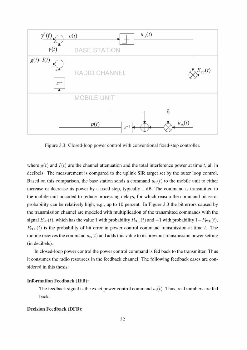
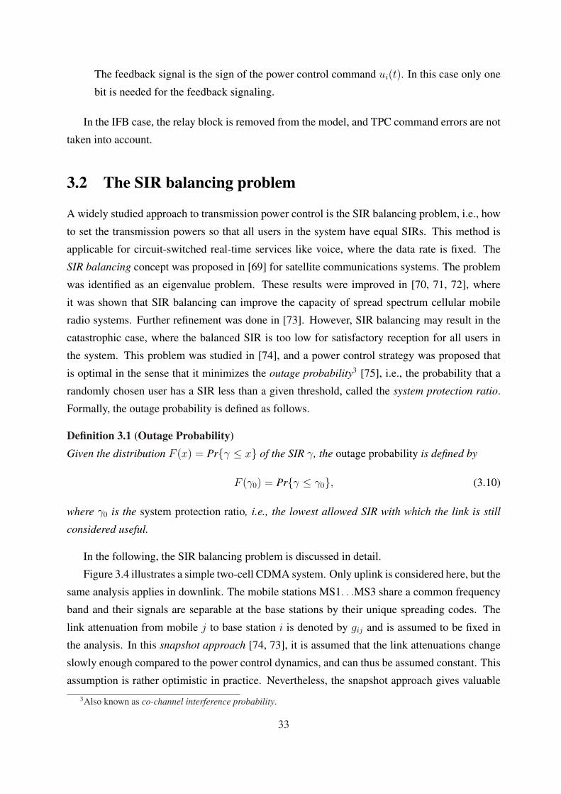
Consider the situation depicted in Figure 3.1. Mobile stations MS1 and MS2 share the same
frequency band and their signals are separable at the base station BS by their unique spreading
1This applies to direct-sequence CDMA (DS-CDMA). In frequency-hopping CDMA (FH-CDMA) the intra-cell
interference can be made very small. In this thesis the focus is on DS-CDMA, where transmission power control is
more critical. Thus throughout the rest of the text, DS-CDMA is referred to simply as CDMA.
23
Page 46
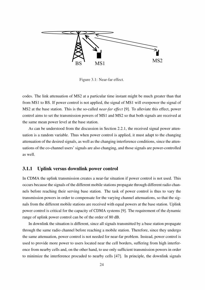
BS MS1MS2
Figure 3.1: Near-far effect.
codes. The link attenuation of MS2 at a particular time instant might be much greater than that
from MS1 to BS. If power control is not applied, the signal of MS1 will overpower the signal of
MS2 at the base station. This is the so-called near-far effect [9]. To alleviate this effect, power
control aims to set the transmission powers of MS1 and MS2 so that both signals are received at
the same mean power level at the base station.
As can be understood from the discussion in Section 2.2.1, the received signal power atten-
uation is a random variable. Thus when power control is applied, it must adapt to the changing
attenuation of the desired signals, as well as the changing interference conditions, since the atten-
uations of the co-channel users’ signals are also changing, and those signals are power-controlled
as well.
3.1.1 Uplink versus downlink power control
In CDMA the uplink transmission creates a near-far situation if power control is not used. This
occurs because the signals of the different mobile stations propagate through different radio chan-
nels before reaching their serving base station. The task of power control is thus to vary the
transmission powers in order to compensate for the varying channel attenuations, so that the sig-
nals from the different mobile stations are received with equal powers at the base station. Uplink
power control is critical for the capacity of CDMA systems [9]. The requirement of the dynamic
range of uplink power control can be of the order of 80 dB.
In downlink the situation is different, since all signals transmitted by a base station propagate
through the same radio channel before reaching a mobile station. Therefore, since they undergo
the same attenuation, power control is not needed for near-far problem. Instead, power control is
used to provide more power to users located near the cell borders, suffering from high interfer-
ence from nearby cells and, on the other hand, to use only sufficient transmission powers in order
to minimize the interference procuded to nearby cells [47]. In principle, the downlink signals
24
Page 47
to different users could be made orthogonal by using proper spreading codes. Unfortunately,
the orthogonality of the downlink signals is lost in practice due to multipath propagation. Thus,
allocating different powers for different users in downlink could cause a near-far situation at the
mobile stations. For this reason, the dynamic range of downlink power control is usually much
smaller than in uplink, typically of the order of 20-30 dB.
The focus in this thesis is on uplink power control, although the proposed algorithms could
also be applied to downlink power control.
3.1.2 Quality measures for power control
A great deal of the work on power control in CDMA cellular systems has focused on how to set
the transmission powers so that all users in the system have acceptable bit-energy-to-interference-
spectral-density ratios (Eb/Io).2 This approach is based on the fairly reasonable assumption that
the bit error probability (BEP) at a receiver is a strictly monotonically decreasing function of
Eb/Io. For instance, BEP Pb of binary phase shift keying (BPSK) modulation in an additive
white Gaussian noise (AWGN) channel is given by [13]
Pb = Q
(√2Eb
Io
), (3.1)
where Q(x) is defined by
Q(x) =1√2π
∫ ∞
x
e−t2/2dt, x ≥ 0. (3.2)
A more relevant case for CDMA cellular systems is the BEP performance of RAKE receiver
in fading channels. Assuming binary modulation, Rayleigh fading channel, and that the RAKE
receiver can coherently combine L paths using maximal ratio combining (MRC) [13], the BEP
performance is [48]
Pb =1
π
∫ π/2
0
L∏
l=1
Il(Γl, g, θ)dθ, (3.3)
where
Il(Γl, g, θ) =
(1 +
gΓl
sin2 θ
)−1
, (3.4)
and
Γl , ΩlEb
Io
(3.5)
2Usually the term bit-energy-to-noise-spectral-density ratio (Eb/No) is used. However, since the CDMA cellular
systems are in practice interference-limited, we prefer to speak about Eb/Io, where Io contains both the interference
and background noise.
25
Page 48
is the average signal-to-noise ratio per bit, corresponding to the lth channel (or resolvable path),
and Ωl is the mean strength of that channel (path). In (3.3), g = 1 for antipodal signals (like
in BPSK) and g = 0.5 for orthogonal signals. Fig. 3.2 shows plots of (3.1) and (3.3) for BPSK
with different numbers of resolvable paths with equal mean strength (flat multipath intensity
profile) and with exponentially decaying multipath intensity profile, where the first path has mean
strength normalized to one, and the mean strengths of the remaining paths decay in steps of 3
dB.
Eb/Io is closely related with another measure, namely the signal-to-interference ratio (SIR),
denoted by γ, such that
Eb/Io = γW
Rb
(3.6)
where W is the transmission bandwidth in Hz and Rb is the data rate in bits/s. The quantity
W/Rb is called the processing gain [11]. When the data rate is fixed, the SIR differs from Eb/Io
by merely a scaling factor.
In digital cellular communication systems, typically, the information to be transmitted is
arranged in strings of bits called frames [49], and error correction coding is applied to each
frame to further decrease the bit error rate (BER) after decoding. A frame is useless if there
are still bit errors in the frame after decoding, and it must be discarded. Hence, depending on
the service, a sufficiently low frame error rate (FER) must be guaranteed. However, long time
delays are needed to obtain reliable estimates of BER or FER. Since the channel conditions can
change very rapidly, these delays might be unacceptably long in practice. Hence most of the
attention in the power control field has been on SIR-based algorithms. Early work concentrated
on algorithms based on received signal strength ([50, 51, 52]). These algorithms typically adjust
the transmission powers inversely proportional to the link gain. In [53] it was shown that partial
compensation of the link gain can give better results than full compensation. In [54, 55] it has
been shown that SIR-based power control offers better performance than signal-strength-based
algorithms. A both SIR-based and signal-strength-based power control algorithm was proposed
in [56] and reported to perform better than plain SIR-based power control.
The frame error information can be used to adjust the target SIR, which a fast TPC algorithm
is trying to achieve. This increases system capacity, since a worst-case setting of the SIR target
is not required.
In addition to the SIR and FER requirements, the delay or latency requirements must be
taken into account. For instance, a voice service tolerates a certain amount of data loss but is
delay-critical, whereas file downloads do not tolerate bit errors at all (erroneous frames must
be retransmitted), but the transmission need not be continuous and must only satisfy some de-
lay limit on the average. The delay tolerances can be utilized in the design of power control
algorithms for nonreal-time services, see e.g. [57].
26
Page 49
0 2 4 6 8 10 12 14 16 18 2010
−6
10−5
10−4
10−3
10−2
10−1
100
Average Eb / I
o per bit
Pb
AWGN
L=10
L=1
(a) Flat multipath intensity profile
0 2 4 6 8 10 12 14 16 18 2010
−6
10−5
10−4
10−3
10−2
10−1
100
Average Eb / I
o per bit
Pb
AWGN
L=10
L=1
(b) Exponentially decaying multipath intensity profile (decay step -3dB).
Figure 3.2: Bit-error probability versus average Eb/Io per bit of BPSK modulation in an AWGN
channel and fading channels with RAKE receiver and maximal ratio combining.
27
Page 50
3.1.3 Open loop, closed loop and outer loop power control
An intuitive way to compensate for the channel attenuation in the uplink would be to measure the
strength of a pilot signal from the downlink, and adjust the transmission power proportionally to
the inverse of this measurement. Since the pilot signal is transmitted at constant power, the vari-
ation of its strength gives information of the downlink link attenuation. This is called open loop
power control. Unfortunately the center frequencies allocated to up- and downlink transmissions
are usually widely separated, and thus the correlation between up- and downlink attenuations is
generally weak. Therefore, the transmission power update of a mobile must be based on feed-
back information of the received SIR at the base station, forming a closed loop between them.
This closed loop power control (or inner loop power control) aims to keep the received uplink
signal power level at a specified target. Moreover, the target must also be varied, because the SIR
requirement for a given BER is not constant, but depends on the radio propagation conditions.
This is the task of the outer loop power control.
Open loop PC is usually used for initial power setting, when the two-way communication
link is not yet established and closed loop is not possible.
Closed loop PC aims to keep the received SIR at a target value. This is what is happening
in the DPC algorithm given in equation (3.19) as discussed later. However, in practice only one
bit is used to signal the received SIR information at a fast rate to track the channel variations.
The transmitter is commanded to increase its power by a fixed step if the received SIR is below
the target, and decrease it otherwise. This kind of algorithm is used in the IS-95 system [58]. In
WCDMA [59, 3] there are some more degrees of freedom, for instance, the possibility to signal
a “no change” command when the received SIR is reasonably close to the target, thus reducing
the “ping-pong”-effect around the target. This idea was exploited in the dynamic step size power
control scheme proposed in [60, 61].
The outer loop control adjusts the SIR target so that a desired FER is guaranteed. A typical
way to do this in practice is to raise the target by a larger step δup when a frame is discarded,
and to decrease the target with a smaller step δdown when a frame is correctly received. This kind
of algorithm was proposed in [62], where they used step sizes δup = Kδ and δdown = δ, where
K is a positive integer. This relation between the step sizes gives the resulting average FER
as FER = 1K+1
. Another algorithm for SIR target adjustment was proposed in [63] for turbo-
coded WCDMA systems. The scheme utilizes the fact that in turbo-decoding, the BER and
FER decrease as the number of decoding iterations increases. Thus, the time required to achieve
reliable BER or FER estimates can be decreased. In [64] another outer-loop PC algorithm was
proposed that is able to detect changes in the multipath channel profile and compensate for errors
in the mapping between FER and SIR target, yielding faster tracking of the channel changes.
28
Page 51
3.1.4 Power control in soft handover
Handover in wireless cellular systems is needed when a mobile user moves from the coverage
area from one cell into that of another cell. In the FDMA and TDMA systems, the handovers are
typically hard handovers, meaning that the connection to the original cell is terminated before
the connection to the new cell is established. In CDMA systems, due to the universal frequency
reuse, a mobile user can be simultaneously connected to several cells. Thus, when a mobile
moves from one cell to another, it can establish connection to the new cell before the connection
to the old cell is terminated. In this case, the mobile is said to be in soft handover [3]. This is
beneficial, since the mobile user can at each time instant use only enough transmission power
to be able to reach one of the base stations to which it is connected. This way the average
transmission power is lower than without soft handover, and less interference is produced to the
other users. However, soft handover increases the radio resource usage in the downlink.
Power control has special implications during soft handover. In UMTS, PC in soft handover
works as follows [59]. In uplink closed-loop PC, the mobile station receives power control com-
mands from all the base stations in the active set (the set of base stations involved in the soft
handover at a given time). It then combines these commands, and based on the combined com-
mand, it adjusts its transmission power. The basic principle is that if any of the base stations
sends a power-down-command, the mobile station decreases its transmission power. The trans-
mission power is increased only if the mobile station receives a power-up-command from all the
base stations in the active set. However, the mobile station can also discard a command in the
case that the reception of that command is poor.
In downlink closed-loop PC, the same PC command sent from a mobile station is received
by all base stations in the active set. Due to errors in the reception of the PC command, the
base station powers can start drifting apart. This is very undesirable, as it destroys the balance
between up- and downlink power levels. A typical way to deal with the power drifting problem
is a scheme called power balancing, where each base station in the active set periodically correct
their transmission powers towards a reference level set by the network [3].
Soft handover has also special implications to the power control algorithms proposed in this
thesis. These are discussed in Chapter 7 with some simulation examples.
3.1.5 Practical aspects on power control considered in this thesis
Many solutions to power control in CDMA systems have been proposed in the literature, as
reviewed later in this Chapter. A lot of work has been devoted to finding optimal (in some sense)
algorithms that may be unpractical to implement, but can be used to derive theoretical bounds
to the performance of the system. Also, a great deal of work has been done to seek distributed
29
Page 52
iterative algorithms that approach the optimal solutions, and are more practical to implement. To
move closer to real implementation of the TPC algorithms, one must take into account a number
of practical issues that limit the capacity gains achievable by TPC:
• Loop delay. The loop delay refers to the overall loop delay in closed loop power control. It
greatly affects the performance of a power control algorithm. This delay is a combination
of delays due to the SIR measurement process, the transmission of the SIR information over
the radio channel, the processing of the SIR information to calculate and adjust the trans-
mission power, and the propagation time after which the new transmission power affects
the next SIR measurement. Therefore the power update is based on outdated information
of the received SIR. This may cause instability in the power control algorithms, leading to
large variations in the interference powers at the receivers and diminished capacity.
• SIR estimation. The received SIR is not known exactly at a receiver, but it must be esti-
mated, and thus there will always be some estimation error. The estimation error can be
made smaller by increasing the averaging time of the measurement, but this might lead to
a longer loop delay, which is undesirable.
• Feedback information accuracy. The information of the SIR at the receiver should some-
how be communicated to the transmitter. An accurate representation of the SIR measure-
ment requires several bits, but this requires more signaling overhead. This form of feedback
is referred to as information feedback (IFB).
A usual case in practice is that only one bit is used to inform the transmitter to either
increase or decrease its transmission power by a fixed amount, typically by 1 dB (e.g. in
WCDMA [59]). This form of feedback is referred to as decision feedback (DFB).
In [65] it was shown that in the case of quantized IFB (the information is represented with
a finite number of bits) the performance gain of adding more bits for the TPC command
becomes less and less when the number of bits is increased and, typically, this saturation
of performance occurs already with a few number of bits. This phenomenon was also
observed in [66], where a differential pulse-code modulation (DPCM) scheme was used to
reduce the required number of bits for the TPC signaling.
• TPC update rate. In CDMA one has to deal with the near-far situation, and thus the update
rate of the power control algorithm must be sufficiently high so that the variations in the
link attenuation can be tracked. Typical update rates are from 800 Hz (used in the IS-95
system [58]) to 1500 Hz (used in WCDMA [59, 3]). Note that the update rate cannot be
arbitrarily high because of the inherent delay imposed by the SIR measurement process.
30
Page 53
Since the available feedback channel bandwidth for power control signaling is limited in
practice, there is a tradeoff between feedback information accuracy and TPC update rate.
Studies have shown that it is generally more beneficial to use high update rate and less in-
formation accuracy than vice versa [67], which supports the choice of 1-bit TPC commands
in UMTS and IS-95.
• Errors in the transmission of feedback information. To minimize the loop delay, the TPC
command bits are sent without error correction coding. Hence the probability of receiving
an erroneous command can be relatively high, e.g. up to 10 %.
• Soft handovers. As discussed in the previous Section, soft handovers have special implica-
tions to the algorithms proposed in this thesis, which is discussed in Chapter 7.
More of these will be discussed in Chapter 4, where new adaptive closed-loop PC algorithms
are proposed for enhancing the power control performance.
3.1.6 The power control model employed in this thesis
The algorithms proposed in this thesis are targeted to improve the TPC performance in the pres-
ence of the practical limitations. The assumption behind the new proposed algorithms is that the
implementation of TPC is done using the combination of open loop, closed loop and outer loop
PC.
The closed loop PC algorithm employed in UMTS and IS-95 systems is a fixed-step power
control (FSPC) algorithm. This type of algorithm has been presented in [68]. It is given by
pi(t + 1) = pi(t) + δsign(γt
i(t)− γi(t))
(3.7)
where all the variables are in decibels, pi(t), γti(t) and γi(t) are the transmission power, SIR
target and measured SIR, respectively, of user i at time t, δ is the fixed step size, and
sign(x) =
1 if x ≥ 0
−1 if x < 0(3.8)
The power control system model is illustrated in Figure 3.3 for uplink. The n-sample delay block
models the power control loop delay (see Section 3.1.5). Note that the integrator in the mobile
unit inherently includes a delay of one sample. Hence the total loop delay is k = n + 1. At time
t the base station measures the uplink SIR. This measurement can be written as
γ(t) = p(t− n) + g(t)− I(t) (3.9)
31
Page 54
z - n
z - 1
+ -
++
g ( t ) - I ( t )
p ( t )
e ( t ) u t x ( t )
E P C ( t )
u r x ( t )
B A S E S T A T I O N
R A D I O C H A N N E L
M O B I L E U N I T
)( ttg)( tg
d
Figure 3.3: Closed-loop power control with conventional fixed-step controller.
where g(t) and I(t) are the channel attenuation and the total interference power at time t, all in
decibels. The measurement is compared to the uplink SIR target set by the outer loop control.
Based on this comparison, the base station sends a command utx(t) to the mobile unit to either
increase or decrease its power by a fixed step, typically 1 dB. The command is transmitted to
the mobile unit uncoded to reduce processing delays, for which reason the command bit error
probability can be relatively high, e.g., up to 10 percent. In Figure 3.3 the bit errors caused by
the transmission channel are modeled with multiplication of the transmitted commands with the
signal EPC(t), which has the value 1 with probability PPCE(t) and−1 with probability 1−PPCE(t).
PPCE(t) is the probability of bit error in power control command transmission at time t. The
mobile receives the command urx(t) and adds this value to its previous transmission power setting
(in decibels).
In closed-loop power control the power control command is fed back to the transmitter. Thus
it consumes the radio resources in the feedback channel. The following feedback cases are con-
sidered in this thesis:
Information Feedback (IFB):The feedback signal is the exact power control command ui(t). Thus, real numbers are fed
back.
Decision Feedback (DFB):
32
Page 55
The feedback signal is the sign of the power control command ui(t). In this case only one
bit is needed for the feedback signaling.
In the IFB case, the relay block is removed from the model, and TPC command errors are not
taken into account.
3.2 The SIR balancing problem
A widely studied approach to transmission power control is the SIR balancing problem, i.e., how
to set the transmission powers so that all users in the system have equal SIRs. This method is
applicable for circuit-switched real-time services like voice, where the data rate is fixed. The
SIR balancing concept was proposed in [69] for satellite communications systems. The problem
was identified as an eigenvalue problem. These results were improved in [70, 71, 72], where
it was shown that SIR balancing can improve the capacity of spread spectrum cellular mobile
radio systems. Further refinement was done in [73]. However, SIR balancing may result in the
catastrophic case, where the balanced SIR is too low for satisfactory reception for all users in
the system. This problem was studied in [74], and a power control strategy was proposed that
is optimal in the sense that it minimizes the outage probability3 [75], i.e., the probability that a
randomly chosen user has a SIR less than a given threshold, called the system protection ratio.
Formally, the outage probability is defined as follows.
Definition 3.1 (Outage Probability)Given the distribution F (x) = Prγ ≤ x of the SIR γ, the outage probability is defined by
F (γ0) = Prγ ≤ γ0, (3.10)
where γ0 is the system protection ratio, i.e., the lowest allowed SIR with which the link is still
considered useful.
In the following, the SIR balancing problem is discussed in detail.
Figure 3.4 illustrates a simple two-cell CDMA system. Only uplink is considered here, but the
same analysis applies in downlink. The mobile stations MS1. . .MS3 share a common frequency
band and their signals are separable at the base stations by their unique spreading codes. The
link attenuation from mobile j to base station i is denoted by gij and is assumed to be fixed in
the analysis. In this snapshot approach [74, 73], it is assumed that the link attenuations change
slowly enough compared to the power control dynamics, and can thus be assumed constant. This
assumption is rather optimistic in practice. Nevertheless, the snapshot approach gives valuable
3Also known as co-channel interference probability.
33
Page 56
BS1
MS1
MS3
BS2
g23
MS2
g22
g21g13
g12
g11
Figure 3.4: Illustration of a two-cell CDMA system with three mobile stations.
insight to the power control problem and the results of the analysis serve as upper bounds for the
performance of various power control algorithms.
Define a base station assignment variable bi so that k = bi if mobile i is served by base station
k. Then the uplink SIR requirement for user i can be expressed as
γi =gbiipi
N∑j=1j 6=i
gbijpj + ηi
=pi
N∑j=1j 6=i
gbij
gbii
pj +ηi
gbii
≥ γti (3.11)
where γi is the SIR at the receiver of the base station that is serving mobile station i, pi is the
transmission power of mobile i, N is the number of mobile stations using the same channel
including the intra-cell and inter-cell users, ηi is the receiver noise power and γti is the uplink SIR
target for user i. Define the vectors p = pi and η = γtiηi/gbii and matrix H = Hij with
elements Hij = γtigbij/gbii when i 6= j and Hii = 0. Now (3.11) can be put in matrix form:
(I −H)p ≥ η (3.12)
where I denotes the identity matrix and the inequality holds component-wise. A minimum-
power solution corresponds to the case where (3.12) is satisfied with equality. This is desirable,
as it saves energy and thus prolongs the mobile station battery life.
Definition 3.2 The problem is said to be feasible if there exists a non-negative power vector p
such that the condition in (3.12) is satisfied.
It has been shown that balancing the SIRs and making the balanced SIR as high as possible
maximizes the minimum SIR in all links [74]. Consider the power control problem in (3.12)
with γti = γt for all i. Define matrix A so that H = γtA. If the interference in the receiver is
34
Page 57
sufficiently high so that the receiver noise can be neglected, the problem can be identified as an
eigenvalue problem:
p = Hp ⇔ 1
γtp = Ap (3.13)
The maximum possible value for γt (denoted by γ∗) is equal to the inverse of the maximum (real)
eigenvalue of A. The corresponding positive eigenvector p∗ is the power vector achieving this
maximum.
If receiver noise cannot be neglected, the optimal power vector is a solution to a set of linear
equations [76]:
p∗ = Hp∗ + η (3.14)
Proposition 3.3 The power control problem in (3.14) is feasible if the largest eigenvalue of the
matrix H , denoted by ρ(H), is less than or equal to one.
ρ(H) is called the spectral radius of the matrix H . The case ρ(H) = 1 can only be met if
the receiver noise is zero, otherwise infinite transmission power would be required. Naturally, in
practice there always exists an upper limit for the transmission power.
Note that ρ(H) can be considered as a measure of the relative system load (see [77]). For
example, a heavily loaded system that is still feasible corresponds to a H matrix with ρ(H) close
to, but less than, unity.
The use of the optimal power vector p∗ results to all users in the system having the same SIR.
If the power control problem is not feasible, this results in the disastrous case that none of the
users achieve the SIR requirement. To prevent this, a removal strategy must be employed, which
removes transmitters from the channel until the power control problem becomes infeasible. The
problem is to select which transmitters to remove. An intuitive approach is to remove those
transmitters that produce the largest interference, i.e., transmitters having the worst link quality.
Several removal strategies have been investigated in the literature ([74, 78, 79, 80]). Note that a
removal of a transmitter from a channel does not necessarily mean that the connection is broken,
but it can be handed over to another channel.
The SIR balancing problem treated here is based on the assumption of constant link attenua-
tions. However, power control must in practice be applied in dynamically changing environment,
where the assumption of constant link attenuations does not hold. In this case the eigenvalue
problem (3.13) corresponds to open-loop control and suffers from poor robustness and high sen-
sitivity. This motivates us to find solutions to power control that are more suitable for application
in a dynamical environment, as is done in Chapter 4.
35
Page 58
3.2.1 Auto-interference
In equation (3.11) the SIR is calculated assuming that all the received power from the desired user
can be considered useful to the receiver. However, due to imperfections in channel equalization,
multipath, transmission nonlinearities, etc., part of this power cannot be used for decoding, and
can be considered interference from the receiver’s viewpoint. This interference is called auto-
interference [81]. In this case the uplink SIR of user i can be expressed as
γi =ζigbiipi
N∑j=1j 6=i
gbijpj + (1− ζi) gbiipi + ηi
(3.15)
where ζi is the fraction of the received power that the receiver can utilize for signal decoding.
The effect of auto-interference has been studied in [81], where it was shown that it lowers the
maximum achievable SIR (γ∗). In [77] it was shown that the auto-interference does not violate
the stability of linear power control algorithms.
The effect of auto-interference is not considered in this thesis. A study on its effect on the
power control algorithms proposed in this thesis is left for future work.
3.2.2 A two-user example
Consider a system with only two mobile stations MS1 and MS2 and two base stations BS1 and
BS2. Assume that MS1 is connected to BS1 and MS2 is connected to BS2. In this case the power
control problem is the following:
γ1 =g11p1
g12p2 + η1
≥ γt1
γ2 =g22p2
g21p1 + η2
≥ γt2
⇒
p1 ≥ γt1
(g12
g11
p2 +η1
g11
)
p2 ≥ γt2
(g21
g22
p1 +η2
g22
) (3.16)
This situation is depicted in Figure 3.5. The feasible region is shaded in the figure, and the
optimal (minimum power) solution p∗ is in the intersection of the two lines. Since p∗ is within
the maximum power limits, the problem is feasible. Consider that user 1 raises its target SIR γt1
while the link attenuations stay unchanged. It is then necessary for it to also raise its transmission
power as seen from (3.16). This in turn forces user 2 to raise its transmission power. Thus it can
happen that the optimal point p∗ moves outside the maximum power limits, thereby making the
problem unfeasible.
36
Page 59
p1
p2
p2,max
p1,max
∗
p
Figure 3.5: Power control problem for two-user case.
3.3 Distributed power control
Solving (3.14) directly is a centralized method, since it requires the information of all the link
attenuations in the system. This is generally not suitable in real implementations, since it would
require extensive signaling overhead. However, it is valuable in determining upper bounds for
the performance of distributed algorithms that can be implemented in practice.
A distributed algorithm uses only local measurements to update the transmission powers.
Hence it is more suitable for practical implementation than a centralized algorithm. Since in this
case a user does not know all the link attenuations, the problem must be iteratively solved. It is
thus necessary to find an iteration that depends only on local measurements, and converges to
the optimal solution reasonably fast (faster than the link gains change). Fast convergence can be
achieved in two ways: by making the iteration time-step smaller, and by designing an iteration
with faster convergence property.
3.3.1 General iterative algorithm
A general iterative algorithm to solve the problem in (3.14) can be found from numerical linear
algebra [82], and is given by
p(t + 1) = M−1Np(t) + M−1η, t = 0, 1, . . . (3.17)
37
Page 60
where M and N are matrices such that p∗ = M−1Np∗+M−1η. By selecting M and N prop-
erly, the iteration in (3.17) will converge so that limt→∞ p(t) = p∗. For example, the selection
M = I and N = H results to
p(t + 1) = Hp(t) + η, t = 0, 1, . . . (3.18)
Writing equation (3.18) component-wise gives
pi(t + 1) = γti
N∑j=1j 6=i
gbij
gbii
pj(t) +ηi
gbii
=
γti
γi(t)pi(t), t = 0, 1, . . . (3.19)
which is the DPC algorithm proposed in [83] (see equation (3.25)).
3.3.2 Convergence of the iterative algorithm
A necessary and sufficient condition for the iteration in (3.17) to converge is the following [82,
84]. Let α1, α2, . . . be the eigenvalues of the matrix M−1N . Then the iteration converges if and
only if maxi |αi| < 1. Consider the DPC algorithm in (3.18). In this case M−1N = H . Hence
the dominant eigenvalue of H , ρ(H), should be less than one. By Proposition 3.3, this ensures
that the SIR requirements can be satisfied for all users. Hence DPC converges to p∗ whenever
the SIR requirements can be satisfied.
The speed of the convergence is very important, since the link attenuations are changing all
the time. For the iteration in (3.17), it can be shown that the smaller the ρ(M−1N), the faster
the convergence. Hence the task is to find M and N such that ρ(M−1N ) < 1 and as small as
possible.
3.3.3 Convergence using standard interference functions
A different way of proving convergence of iterative algorithms was developed in [85] and ex-
tended in [86]. There the iteration is formulated by defining an interference function I(p) such
that
p(t + 1) = I (p(t)) (3.20)
The standard interference function framework gives a sufficient but not necessary condition for
convergence of the iteration in (3.17). The following definition and proposition summarize this
framework.
38
Page 61
Definition 3.4 ([85]) An interference function I(p) is called standard if for all non-negative
power vectors the following properties are satisfied:
• I(p) > 0 (positivity)
• p ≥ p′ ⇒ I(p) ≥ I(p′) (monotonicity)
• ∀α > 1, αI(p) > I(αp) (scalability)
(3.21)
Proposition 3.5 ([85]) If the power control problem is feasible and I(p) is a standard interfer-
ence function, then for any initial non-negative power vector p the iteration in (3.20) converges
to the unique non-negative fixed point p∗.
Recently, a generalization of the standard interference function method has been presented in
[87, 88]. They identified a key condition for convergence of an iterative function:
Definition 3.6 ([87, 88]) Two-sided scalability:
For all α > 1, 1αp ≤ p′ ≤ αp implies 1
αI(p) < I(p′) < αI(p).
Proposition 3.7 (Theorem 1 in [87]) Given a two-sided scalable iterative function I(p), if a
fixed point p∗ = I(p∗) exists, then that fixed point is unique and the iteration p(t + 1) = I(p(t))
converges to p∗ under both synchronous and totally asynchronous update model.
3.4 A survey of power control algorithms and state of the art
Here the goal is to give an overview of the research efforts made on power control algorithms in
the past and to present the state of the art of this widely studied field. The presentation is divided
into fours parts and gives a somewhat – although not entirely – chronological view on how the
research has evolved from the past to the present.
3.4.1 Distributed SIR balancing algorithms
Distributed versions of the SIR balancing problem draw a lot of attention in the 1990’s. The
starting point was to find iterative algorithms that would be suitable for distributed operation,
and would solve the eigenvalue problem (3.13) in the noiseless case, or the set of linear equa-
tions (3.14) in the noisy case. The underlying assumption was that the channel power gains
would change slowly compared to the dynamics of the power control iterations, and thus the
convergence was mainly studied in a static “snapshot” scenario.
The first proposal was the Distributed Balancing (DB) algorithm proposed in [89]. It is
described in the following.
39
Page 62
The Distributed Balancing (DB) Algorithm:
pi(t + 1) = βpi(t)
(1 +
1
γi(t)
), β > 0, t = 0, 1, . . . , (3.22)
♦For a feasible system, the DB algorithm converges to the optimal power vector p∗ with prob-
ability one4 (see [89]). However, it suffers from poor convergence speed. Moreover, an improper
selection of parameter β may result in ever-increasing (or decreasing) powers. The correct se-
lection of β requires a normalization procedure, which is not possible to do in a completely
distributed manner.
An improvement to the DB algorithm in terms of convergence speed was proposed in [90].
They proposed a modified version of the DB algorithm and called it the Distributed Power Con-
trol (DPC) algorithm. However, since the term DPC is used for another algorithm (described
later), the algorithm of [90] is called the Modified DB (M-DB) Algorithm. It is described as
follows.
The Modified DB (M-DB) Algorithm:
pi(t + 1) = βpi(t)
γi(t), β > 0, t = 0, 1, . . . (3.23)
♦The convergence of the M-DB algorithm to the optimal power vector and SIR balance has
been proven in the noiseless case ([90]). Also, the convergence speed was shown to be faster
than with the DB algorithm. This was also analytically shown in [76]. However, the problem of
cleverly choosing β still remained.
The problem with the normalization procedure was avoided in the algorithm proposed in [91],
the Fully Distributed Power Control (FDPC) Algorithm. It is given in the following.
The Fully Distributed Power Control (FDPC) Algorithm:
pi(t + 1) = pi(t)min (γi(t), β)
γi(t), t = 0, 1, . . . (3.24)
♦Clearly, β → ∞ corresponds to constant power case (no power control). For very small values
of β the FDPC algorithm approaches the M-DB algorithm. The FDPC algorithm can achieve
4Convergence with probability one here is based on the assumption that the link gains in matrix H are stochastic
variables, and the matrix has therefore full rank. This assumption is feasible since the link gain in a wireless
communication channel is inherently a stochastic variable.
40
Page 63
SIR balance with probability one in the noiseless case, if β ≤ γ∗, where γ∗ is the maximum
achievable SIR in the system (see Section 3.2). A drawback of the algorithm is that if β < γ,
where γ is the system protection ratio, the powers are ever-decreasing, which is a problem in the
noisy case.
The algorithm proposed in [83] finally solved the problem of choosing β of the M-DB al-
gorithm in the noisy case. They identified β in the noisy case to be the target SIR which the
algorithm is trying to achieve. This algorithm is called the Distributed Power Control (DPC)
Algorithm in this thesis. It is described as follows.
The Distributed Power Control (DPC) Algorithm:
pi(t + 1) = pi(t)γt
γi(t), t = 0, 1, . . . (3.25)
♦From control theory viewpoint, the DPC algorithm is an integrating P-controller. The conver-
gence of the DPC algorithm in the case where the power updates occur asynchronously was
proven in [92]. The DPC algorithm has received wide attention in the research community since
it was published.
In all practical systems the transmission powers are limited so that
0 ≤ p ≤ pmax (3.26)
where 0 is a vector with all-zero elements and pmax = [pmax1 , pmax
2 , . . . , pmaxN ]T denotes the max-
imum transmission power of each transmitter. To take these limitations into account, the dis-
tributed constrained power control (DCPC) algorithm was suggested in [93]. The algorithm
converges in a geometric rate [86]. It is defined in the following.
The Distributed Constrained Power Control (DCPC) Algorithm:
pi(t + 1) = min
(pmax
i , pi(t)γt
i
γi(t)
), t = 0, 1, . . . (3.27)
where pmaxi is the maximum allowed transmission power of transmitter i.
♦With DCPC it can happen that some transmitters are transmitting with the maximum power,
thus producing maximum interference to other users, but still do not achieve their SIR target.
Therefore it might be beneficial to lower the transmission power when link quality is bad. With
this in mind, the following more general algorithm has been proposed in [94] that has DCPC as
a special case:
41
Page 64
The Generalized Distributed Constrained Power Control (GDCPC) Algorithm:
pi(t + 1) =
γti
γi(t)pi(t) if γt
i
γi(t)pi(t) ≤ pmax
i
p′i if γti
γi(t)pi(t) > pmax
i
, t = 0, 1, . . . (3.28)
where 0 ≤ p′i ≤ pmaxi .
♦It was shown in [94] that this algorithm converges to the optimal power vector p∗ provided that
the system in (3.14) has the optimal solution p∗ in the power range given by (3.26).
3.4.1.1 Discrete transmission powers
All the above algorithms assume that the transmission power can be selected from a continuous
range. Systems with quantized transmission powers are considered in [95, 96]. They proposed
the Distributed Discrete Power Control (DDPC) Algorithm, which is based on simple quanti-
zations of the transmission powers calculated by the DCPC algorithm. The same problem was
addressed also in [97], where the problem is generalized to an integer programming problem
with certain constraints. In [98] a distributed discrete power control method based on stochastic
learning was proposed in a game theory framework for wireless data networks.
3.4.2 Aiming for faster convergence
The DPC algorithm was the first practical one to solve the problem of SIR balancing in a fully
distributed manner. After that many efforts have been devoted for finding algorithms with faster
convergence. For algorithms based on the general iterative algorithm (see Section 3.3.1), faster
asymptotic average rate of convergence [99] is achieved by finding an iteration matrix M−1N
with smaller spectral radius ρ(M−1N ).5 I has been shown [99, 17] that ρ(M−1N) for the DPC
algorithm is smaller than for the DB algorithm, thus the DPC algorithm has faster convergence.
For some algorithms it is difficult or even impossible to find the rate of convergence analytically,
and one must resort to simulations to study the convergence. Fast convergence is important,
since the power control algorithms are in practice operating in a dynamical system with random
variations. However, the convergence of the algorithms has been mainly studied in a static envi-
ronment, assuming that the variations in the radio channel power gains are slow in comparison
with the power control dynamics and can thus be neglected.
5Of course the iteration matrix must be selected so that it enables a distributed implementation of the algorithm,
see the discussion in [99] page 32.
42
Page 65
In [100] a power control algorithm is proposed with faster convergence properties than the
DPC algorithm. The algorithm differs from the first-order algorithms described above in the
sense that it requires the current and the previous power levels to calculate the next one. The
scheme is called the Constrained Second-Order Power Control (CSOPC) Algorithm. It is de-
scribed as follows.
The Constrained Second-Order Power Control (CSOPC) Algorithm:
pi(t + 1) = min
(pmax
i , max
(0, pi(t)ω(t)
γti
γi(t)+ (1− ω(t))pi(t− 1)
)),
t = 1, 2, . . .
(3.29)
where ω(t) is called the relaxation factor, and is a decreasing sequence such that 1 <
ω(1) < 2 and limt→∞ ω(t) = 1.
♦From control theory viewpoint, the CSOPC algorithm is an integrating PD-controller with van-
ishing D-part. In the simulations of [100] the authors have used ω(t) = 1 + 11.5t , t = 1, 2, . . ..
Another algorithm with faster convergence properties is proposed in [101, 17]. The algorithm
is called the Multi-Objective Distributed Power Control (MODPC) Algorithm, and is based on
multi-objective optimization framework. Its convergence was shown to be faster than that of the
DCPC. The MODPC algorithm is described as follows.
The Multi-Objective Distributed Power Control (MODPC) Algorithm:
pi(t + 1) = min
(pmax
i , pi(t)λpmin
i + (1− λ)γti
λpi(t) + (1− λ)γi(t)
), t = 0, 1, . . . (3.30)
where pmini is the minimum allowed transmission power of transmitter i, and λ ∈ [0, 1] is a
weighting parameter.
♦Note that selecting λ = 0 yields the DCPC algorithm. The MODPC algorithm was extended to
jointly control power and data rate in [102]. A drawback of the MODPC algorithm is that for
λ > 0 the algorithm converges to a smaller SIR balance than the DCPC algorithm (here it is
assumed that the power control problem is feasible within the power limits). To see this, rewrite
(3.30) in steady-state case, resulting in:
pi = piλpmin
i + (1− λ)γti
λpi + (1− λ)γi
(3.31)
⇒ γi = γt +λ
1− λ(pmin
i − pi) ≤ γt. (3.32)
Therefore, unless pi = pmini or λ = 0, then γi < γt.
43
Page 66
0 5 10 15 20 25 30 350
0.2
0.4
0.6
0.8
1
Iteration number
|| p
− p
* ||
DBDCPCCSOPCMODPC
Figure 3.6: Convergence of the norm of the difference between the power vector and the optimal
power vector p∗ (equation (3.14)) in multiuser snapshot simulation (80 users).
3.4.2.1 Convergence example
Fig. 3.6 shows the simulated convergence of the DB, DCPC, CSOPC and MODPC algorithms in
a multiuser case with 80 users, averaged over 100 realizations. The CSOPC clearly outperforms
the other algorithms in terms of convergence speed. The MODPC has also fast convergence, but
it converges to a slightly different power vector than the other algorithms, as discussed in the
previous Section. The DCPC has only slightly faster convergence than the DB algorithm.
3.4.3 Power control for dynamical environment
The methods presented above are mostly based on finding the solution to the eigenvalue problem
(3.13) or the set of linear equations (3.14) in a distributed manner. Later on, more efforts were
put to the problem of controlling the powers in dynamic channel conditions and in the presence
44
Page 67
of non-idealities such as loop delays and feedback bandwidth restrictions.
Adaptive fuzzy control -based power control algorithms are proposed in [103, 104]. The
fuzzy rule base in the algorithms is based on assumptions on the channel fading characteristics.
Specifically, it is assumed that the channel fading process can be modeled as a piecewise second-
order system. Based on the rule base, they use a fuzzy proportional integral (PI) controller for
power control. The system can be designed to take the loop delay into account to enhance the
robustness of the algorithms. The main drawback of these algorithms is that the channel behavior
must be estimated in advance to construct the fuzzy rule base (see also [105]). Also the limited
feedback bandwidth is not taken into account.
The problem of compensating the loop delay in closed-loop power control has been addressed
in [106, 107, 77]. There the authors identified the problems that the loop delay may cause with
various power control algorithms, including the DCPC and FSPC algorithms (this is elaborated
in Chapter 4). They proposed a time delay compensation (TDC) scheme to remove the effect of
delays in the output powers from the measurements in the closed-loop power control. The TDC
scheme is based on the fact that after issuing a power control command, the resulting output
powers are known to the algorithm, and can be precalculated and used in the measurements. To
elaborate, let γi(t) be the SIR at the receiver of user i in decibels. Then
γi(t) = pi(t− n) + gii(t)− Ii(t), (3.33)
where pi(t) is the transmit power of user i at time t, gii(t) is the link gain between the transmitter
and receiver of user i at time t, Ii(t) is the interference power at the receiver of user i at time
t, and n is the additional loop delay in samples.6 Consider the following general power control
algorithm:
pi(t + 1) = pi(t) + Riγti(t), γi(t) (3.34)
where Riγti(t), γi(t) is some arbitrary power control mechanism. With TDC the algorithm gets
the following form:
i) Adjust measurements: γi(t) = γi(t) + pi(t)− pi(t− n).
ii) Issue PC command: si(t) = Riγti(t), γi(t).
iii) Monitor output powers: pi(t + 1) = pi(t) + si(t).
(3.35)
Time delay compensation is a simple scheme, which can effectively cancel the loop delay.
It has, however, two drawbacks. One is that the loop delay must be known. This is in principle
a problem in cellular CDMA systems, where the loop delay is usually known due to the known6A general iterative power control algorithm as in (3.17) itself has a delay of one sample, since measurements at
time t are used to update powers at time t + 1. We use k to refer to the total loop delay including this internal delay.
Thus, n = k − 1.
45
Page 68
frame structure of the system. However, there are cases when there are uncertainties in the loop
delay. The other drawback is that since the TDC method relies on the knowledge of the PC
actions taken by the transmitter after receiving the PC commands, it cannot be used when the
mobile station is in soft-handover [77]. The loop delay issue is discussed more thoroughly in
Chapter 4, where algorithms are designed to take the loop delay into account in cases where it is
known, and also in cases when it cannot be guaranteed to be known.
In [108] the closed-loop PC is considered with feedback bandwidth constraints as an instance
of the classical quantization problem. In this scheme, the receiver estimates the variance of the
PC misadjustment, which is used to optimally quantize the power control command. The scheme
relies on the assumption that the PC misadjustment is log-normally distributed, which is also the
assumption used in the algorithms proposed in this thesis in Chapter 4. Thus, the minimum-
mean-square-error (MMSE) optimization criterion is used for the quantizer. The estimated vari-
ance must be communicated to the transmitter for the reconstruction, which is a drawback of the
scheme. The authors also propose a loop filter to be used in the transmitter for exploiting the
time-correlation of the PC misadjustment. Thus, in the presence of loop delays, the loop filter
should be designed so that the loop remains stable. In Chapter 6 of this thesis, new methods
are proposed to enhance the closed-loop PC performance at the transmitter side. These methods
utilize only the received 1-bit TPC commands and do not require any other information.
3.4.4 Predictive power control
Various forms of predictive power control have been proposed in the literature to exploit the time
correlation of the channel states, and to tackle the loop delay problem. The usual approach in
predictive power control has been to predict the received signal power or SIR [109, 110, 111],
channel state [112, 113, 114, 115, 116], or the next transmission power that should be used by
the transmitter [117, 118], using linear K-step-ahead predictors based on current and previous
values of the predicted signal, or neural networks.
In [109, 110, 111] prediction in the received signal power with polynomial predictors is pro-
posed. The methods are based on the assumption that the channel power gain follows polynomial
curves. Recall that this was also the assumption used in the fuzzy control schemes proposed in
[103, 104]. As in those schemes, the predictive schemes of [109, 110, 111] need to estimate the
channel behavior beforehand to select the polynomial predictors.
The channel state predictors utilized in [112, 113, 114, 115] are of the form
g(t + 1) =N∑
i=0
w(i)g(t− i), (3.36)
where g(t) is the channel power gain at time t, w(i), i = 0 . . . N are the weights of the prediction
46
Page 69
filter and N is the order of the filter. The weights are updated using some adaptive algorithm
such as the Recursive Least Squares (RLS, [113]), Least Mean Squares (LMS, [114, 115]) or
Normalized Least Mean Squares (LMS, [112]) algorithm.7 In [116] a K-step-ahead prediction
algorithm is proposed, where the samples are iteratively predicted one sample ahead, each time
utilizing the already predicted values to predict the next sample ahead, until the required number
of predicted samples is reached. These algorithms require that the channel state (power gain) can
be measured. In particular, the channel power gain is equal to the received power divided by the
transmission power. Thus, it is assumed that the channel power gain can be calculated from the
received power measurements and the transmission power commands sent to the transmitter in
the feedback channel [112]. However, as already discussed, the feedback channel for the power
control command is typically a relatively unreliable channel, and thus the estimated channel gain
can easily become biased.
In [117, 118], a centralized predictive power control algorithm based on achievable SIR is
proposed. It is assumed that the link gains of the entire system can be estimated, and the optimal
power vector (see (3.13)) is calculated based on the link gain matrix. A similar prediction as in
(3.36) is applied to estimate the next optimal power vector based on previously calculated power
vectors. Two schemes are presented, where one uses an individual predictor based on the RLS
algorithm for each user, and the other uses a global predictor based on a neural network to predict
the entire power vector. The main problem with these schemes is that they, require an enormous
amount of signaling overhead, which makes them difficult to implement in practice.
3.4.5 Discussion
It is clear that the design of power control for CDMA systems is not a simple problem. Many
different solutions have been proposed for enhancing various aspects of power control. However,
there are still questions that have not been answered. This thesis concentrates on finding answers
to the following questions:
• How to minimize PC misadjustment in closed-loop power control and simultaneously com-
pensate for the loop delay to enhance the capacity of the system?
• How to do this without increasing power control signaling bandwidth requirements?
• How to deal with unknown or varying loop delay?
In Chapters 4–7, solutions to these problems are proposed.
7See [119, 120] for information about these adaptive algorithms.
47
Page 70
3.5 Power control in real-time versus nonreal-time and multi-
rate services
The SIR balancing concept has the goal of maximizing the number of users in the system. If
the users are real-time users requiring constant bit rates, this is a good strategy for maximizing
capacity. However, as the cellular systems evolve to the next generation, the variety of services
will be considerably different than those of the previous systems. In addition to the familiar
real-time voice, there will be both real-time and nonreal-time services with different data rates.
Hence, maximizing the data throughput instead of the number of users might be more interesting
from the operators’ point of view. Of course the delay requirements must be fulfilled, as merely
maximizing throughput would be achieved by just letting the user with the best instantaneous
link quality to transmit [121, 122].
Since CDMA is interference limited, any decrease in the transmission power of one user is
directly advantageous for other users due to decreased interference. If the link quality between
a transmitter and a receiver is bad, high transmission power is needed to satisfy the SIR require-
ments. This produces high interference to other receivers, and their serving transmitters must
also increase their powers in order to cope with the increased interference.
In nonreal-time services the data rate must only be satisfied on the average sense, and there-
fore the instantaneous data rate can be considerably varied. This allows the TPC algorithm even
to cut off the transmission when the link quality is bad, and to transmit at a high data rate when
the link quality is good [122]. Thus, the situation as compared to conventional TPC designed for
real-time services is reversed: the transmission power should be small when link quality is low,
and vice versa. Since the time dimension can be utilized in the optimization, there is potential for
significant capacity gain by minimizing the total transmitted energy instead of power. This can
be accomplished by scheduling the data transmissions properly [57].
To elaborate this, consider a set of users requiring individual data rates. Using (3.6) and
(3.11) the effective data rate of user i is written as:
Rb,i =W
(Eb/Io)i
γi(p) (3.37)
where γi(p) is the received SIR of user i with the power vector p and (Eb/Io)i is the Eb/Io
requirement for user i for achieving the data rate Rb,i. Let the maximum transmission power
vector for the users be pmax = (pmax1 , pmax
2 , . . . , pmaxN ).
Definition 3.8 ([84, 57]) A rate vector Rb (pmax) = (Rb,1, Rb,2, . . . , Rb,N) is instantaneously
achievable if there exists a non-negative power vector p ≤ pmax such that Rb,i ≤ W(Eb/Io)i
γi(p)
for all 1 ≤ i ≤ N .
48
Page 71
Definition 3.9 ([84, 57]) A rate vector R∗b (pmax) =
(R∗
b,1, R∗b,2, . . . , R
∗b,N
)is achievable in the
average sense if it may be expressed as R∗b =
∑i λiRb,i, where λi ∈ [0, 1],
∑i λi = 1, and all
the Rb,i are instantaneously achievable rate vectors.
Thus, different rate vectors can be assigned a fraction of time (or frequency) yielding the
required rate vector on the average. Assume that each link i requires a minimum data rate Rminb,i .
Any excess data rate is potentially consumed, and thus paid for, by the user. It is the interest of
the operators then to provide as much excess data rate as possible. For nonreal-time services,
therefore, the following optimization problem is of interest:
maxN∑
i=1
R∗b,i(pmax)
subject to R∗b,i(pmax) ≥ Rmin
b,i ,∀i(3.38)
3.6 Power control and other radio resource management
Optimizing power control alone is not always the best way to enhance capacity. By understanding
the relations between power control and other radio resource management (RRM) functions, one
can design more efficient algorithms by combining them in an ingenious way. For instance, base
station assignment is closely related to the power control problem. The integration of base station
assignment and power control was studied in [123]. They considered the following minimum
transmission power (MTP) problem:
The Minimum Transmission Power (MTP) Problem:minimize
∑i pi
subject to
gbiipi ≥(∑
j 6=i gbijpj + ηi
), 1 ≤ i ≤ N
pi ≥ 0, 1 ≤ i ≤ N
bi ∈ 1, . . . , M, 1 ≤ i ≤ N ,
where N and M are the number of users and the number of base stations in the system,
respectively.
♦They showed that by optimizing over all base station assignments and power vectors, there exists
a unique minimum power vector that solves the MTP problem. They also presented iterative
algorithms that solve the MTP problem in a distributed manner.
The task of admitting new users in the system is called admission control. In [124] an active
link protection scheme was proposed, in which a candidate user to be admitted to the system
49
Page 72
starts up with small power, and gradually increases it by a fixed step, while the other users update
their powers with the DPC algorithm, but increasing their SIR targets with the same fixed power-
up step. This way the SIRs of the active links are protected from falling below their predefined
targets. The scheme is called Distributed Power Control with Active Link Protection (DPC-ALP)
Algorithm, and is formally given as follows.
The Distributed Power Control with Active Link Protection (DPC-ALP) Algorithm:
pi(t + 1) =
δγti
γi(t)pi(t) if γi(t) ≥ γt
i
δpi(t) if γi(t) < γti
, t = 0, 1, . . . (3.39)
where δ > 1 is the power-up step.
♦Power constraints with the DPC-ALP scheme are considered in [125]. During the admission of a
new user it may happen that the transmission power of the active users may achieve the maximum
power limit, causing their SIRs to fall below the target. As a remedy, a distress signaling is
proposed, where an active user approaching the power limit sends a distress signal to the new
users that are then blocked and cease their transmission.
A drawback of the DPC-ALP scheme is that the system capacity is diminished due to the
increase in the SIR targets of the active links during admission of new users. Another algorithm
is proposed in [126] that does not suffer from capacity loss. The algorithm is called the Soft and
Safe Admission Control (SAS) Algorithm. A drawback of SAS is that while it is fast in admitting
a new mobile, it is very slow to reject it.
Combined power and rate control is interesting for services with heterogeneous bit rates and
quality requirements as discussed in the last section (see also [99, 127, 128]). Other methods that
have been considered jointly with power control include smart antennas and beamforming, where
there are more degrees of freedom in the optimization of the algorithms [129, 130, 131, 17].
Without going into details about beamforming (for information about beamforming, see [132]),
typically the joining of power control and beamforming is done in two phases: in the first phase,
the beamforming weights are updated to maximize SIR, and in the second phase, the maximized
SIR is used in power control calculations. Hence, any SIR-based power control method could
then be used in combination with beamforming.
Recently, the joining of power control with spreading code allocation has been an active
research topic in the literature. In these schemes, the spreading codes are allocated so as to
minimize the interference, and power control is used again to ensure that the specified target SIR
is achieved [133, 134].
50
Page 73
3.7 Views into the future
The ultimate goal of radio resource management is to maximize the network capacity without
sacrificing the satisfaction of the users too much. Efficient transmission power control is essen-
tial in CDMA cellular systems for achieving these goals. The efficiency of TPC depends on
its ability to control the interference inherent in wireless multiuser systems. However, there are
other methods for combating the multiple access interference in CDMA. One of these methods is
multiuser detection (MUD). An optimal MUD-based receiver would theoretically eliminate the
need for power control completely! In practice, however, an optimal MUD-receiver would be too
complex, and suboptimal solutions must be used that are not completely immune to interference,
and TPC can still provide additional gain. Using only TPC provides a much cheaper way of con-
trolling interference. This situation might change in the future, as the microtechnology evolves
very fast and more efficient chips become available.
51
Page 75
Chapter 4
Adaptive closed-loop power control
4.1 Introduction
In this chapter new algorithms for closed-loop power control in CDMA systems are proposed.
As discussed in Chapter 3, the closed-loop PC aims to keep the received SIR in a target set
by an outer-loop controller, by sending feedback signals to the transmitter. To minimize the
power control signaling, practical CDMA systems typically employ a simple fixed-step (decision
feedback) power control scheme that does not take advantage of the power control command and
measurement histories. However, due to the time variation of the radio channel and interference
seen by a receiver, and the loop delay (see Chapter 3), the command may already be outdated
by the time it can be applied in the transmitter. Even if the feedback information signals are
not quantized, the loop delay can cause serious problems to power control algorithms if it is not
properly taken into account. The new approach is to model the power control process with a
linear process model, and to design an adaptive self-tuning controller to minimize the variance
of the process output, which is the SIR at the receiver or its distance to SIR target. Decision
feedback versions of the algorithms are also provided. Those algorithms are able to mitigate the
undesirable effects of the loop delay without any increase in power control signaling.
The proposed algorithms are evaluated via computer simulations using the simulator de-
scribed in Appendix A. Examples of simulation results are given throughout the Chapter at
appropriate points.
This chapter is related to publications [135, 136, 137, 138, 139, 140, 141].
4.2 Motivation for adaptive controller approach
As discussed in Chapter 3, many of the distributed iterative power control algorithms proposed
in the literature can be put in the general form (3.17). These algorithms have been derived from a
53
Page 76
rather theoretical viewpoint, where it is assumed that the iteration converges fast enough so that
the channel attenuations can be assumed to be constant during this time. In practice, however,
there are several factors that may render this assumption incorrect, as discussed in Section 3.1.5.
The delays involved in the SIR measurement process, transmission and the processing of the
algorithm itself can be long enough so that the channel as well as interference conditions might
be considerably changed during the delay. As seen later in simulations, this might be disastrous
for the performance of the PC algorithms that do not take the loop delay into account. The loop
delay is tackled in this thesis through linear prediction, which has been shown also in the work
by others to be an effective way to increase power control performance in the presence of loop
delays, as discussed in Section 3.4.4. Typically, the prediction is applied to the received signal-
to-interference power ratio (SIR) based on its previous measurements, and the predicted SIR
value is compared to the SIR target, which is set by outer-loop power control. In the proposed
algorithms of this Chapter, a different approach has been taken. A linear model of the power
control process is first constructed, and a self-tuning controller is designed to control the model.
The loop delay can be included in the model, and the controllers are designed to minimize a cost
function that includes k-samples-ahead prediction of the process output (in this case, either the
SIR or the difference of SIR and SIR target), where k equals the loop delay in samples. In this
way the information of both the previous estimates of the SIR and the previous control commands
can be utilized to achieve better performance. In Section 4.9 algorithms are proposed to take into
account situations where the loop delay might not always be known.
Another issue is the feedback bandwidth needed in closed loop power control for the power
control command transmission. In practical systems the power control command is typically one
bit long, allowing only power up / power down -commands to be fed back to the transmitter.
This one-bit feedback is also called decision feedback (DFB). In order to take this limitation into
account with the proposed algorithms, some modifications are needed to the standard self-tuning
control methods to make them work in a decision feedback manner.
Finally, in order to follow the changes of the dynamical radio environment, the parameters of
the linear model are estimated in real time with an adaptive algorithm.
The assumption behind the new proposed algorithms is that the SIR target is provided via
outer loop PC, and the task of closed-loop PC is thus to follow that target. Thus, from viewpoint
of system capacity, the goal is to enhance the target tracking capability of the closed-loop PC,
which enables the outer-loop PC to reduce the SIR target, which in turn increases capacity due
to diminished interference. This goal is elaborated in Section 4.2.3 in more detail.
54
Page 77
F o r w a r d l i n k s l o t sa t t r a n s m i t t e r
F o r w a r d l i n k s l o t sa t r e c e i v e r
F e e d b a c k l i n k s l o t sa t r e c e i v e r
F e e d b a c k l i n k s l o t sa t t r a n s m i t t e r
t - 1 t t + 1
P r o p a g a t i o n d e l a yT i m e o f f s e t
P r o p a g a t i o n d e l a y
S l o t
S I R e s t .T P C c o m m a n d
TPC
TPC
TPC
A p p l yT P C c o m m a n d
Figure 4.1: Example of power control timing in WCDMA [59]. To permit a short TPC delay, the
frame timing of the feedback link is offset from that of the forward link. The receiver receives
the slot that is transmitted at time t − 1 after a propagation delay. The receiver then estimates
the SIR from a number of pilot and/or data symbols, derives a TPC command, and transmits the
command in the feedback link to the transmitter. The transmitter receives the command after a
propagation delay and adjusts its transmission power for the next slot according to the command.
Thus the loop delay is one PC period. If the delays due to SIR estimation and TPC command
processing are longer, the command may not reach the transmitter within one-slot-time. In this
case, the transmission power is changed for the slot that is transmitted at time t + 1, resulting in
a loop delay of two PC periods.
4.2.1 Loop delay example
A typical loop delay situation encountered in WCDMA is illustrated in Figure 4.1. Since the
power control signaling is standardized, the loop delays are in principle known exactly. The slot
at time t − 1 is transmitted using power p(t − 1). The receiver measures the SIR γ(t) over a
number of pilot and/or data symbols and derives a TPC command. The command is transmitted
to the transmitter in the feedback link and the transmitter adjusts its transmission power according
to the command. If the SIR measurement window, processing delays and propagation delays are
short enough, as in the example in Figure 4.1, the loop delay can be as short as one PC period.
Otherwise, the TPC command cannot be applied at the transmitter within one-slot-time, resulting
in longer loop delays. Note that the SIR estimation window affects the PC timing. If a short
55
Page 78
window is used, the loop delay can be shorter, but the SIR estimation becomes more unreliable.
To elaborate, consider the uplink case. The number of pilot bits in WCDMA uplink Dedicated
Physical Control Channel (DPCCH) slot can be from 3 to 8 [142]. The duration of one slot is 667
µs, and there are 10 bits in a DPCCH slot, so one pilot bit duration is 66.7 µs. Assuming that all
available pilot bits are used for SIR estimation, the averaging time of the estimation ranges from
200 µs to 534 µs. The uplink frame is delayed from the downlink frame by 1024 chips (267 µs),
measured at the mobile station antenna, so the time offset in Figure 4.1 is 667 µs−267 µs−2τp =
400 µs − 2τp, where τp is the propagation delay. Looking at Figure 4.1 it is seen that the one-
slot loop delay requires that, starting from the beginning of the first pilot bit at the receiver, the
TPC command must be ready within the time offset plus the offset of the TPC field from the
beginning of the feedback slot. This limits the time available for SIR estimation and the available
processing delay. Depending on the downlink slot format, the offset of the TPC command from
the beginning of the slot can range from 0 to 130 µs [142]. Thus, from the beginning of the first
pilot bit at the receiver, the time available for SIR measurement, TPC command generation and
its placement into the downlink slot ranges from 400 µs−2τp to 530 µs−2τp. The longest signal
path in a typical WCDMA system can be 5 km, so the maximum propagation delay is about 17
µs. Thus, in the worst case, there will be (400 − 34) µs = 366 µs time for SIR measurement,
TPC command generation and its placement into the downlink slot. If the TPC command is not
ready within this time, it must be delayed to the next slot.
4.2.2 Problems caused by the loop delay
It has been shown that if not properly controlled, the loop delay can cause serious problems to
the power control algorithms [106, 107, 77, 140]. Some IFB algorithms, like the widely known
DCPC algorithm, can even become unstable in the precence of loop delays.
Since the maximum power adjustment is limited in the FSPC, the loop delay does not destroy
the performance of the algorithm, but considerably increases the variance of the SIR at the re-
ceiver minus the SIR target. It has been shown [143, 77] that the FSPC algorithm converges to a
bounded region ∣∣γti − γi(t)
∣∣ ≤ 2δk (4.1)
provided that the power control problem is feasible within this margin. Here δ is the step size of
the algorithm and k is the total loop delay. Thus, longer loop delays lead to larger convergence
bounds.
It can be shown [77] that with the FSPC algorithm time delay compensation (TDC, see Sec-
tion 3.4.3) the PC misadjustment converges to∣∣γt
i − γi(t)∣∣ ≤ δ(k + 1) (4.2)
56
Page 79
which should be compared to (4.1). However, the fact that the bound is tighter does not imply
that the variance of the PC misadjustment is smaller.
Figure 4.2 shows how an additional loop delay of one sample, so that k = 2, affects vari-
ous non-predictive PC algorithms without time delay compensation. In the simulation, only the
randomly selected observed user is power controlled with different algorithms, while all other
users use the FSPC algorithm. The speed of the selected user is 5 km/h. The total loop delay k is
increased from one to two at sample number 300. It is seen that all the IFB-algorithms become
unstable after this change. The FSPC algorithm remains stable, but the amplitude of the envelope
of the SIR variation grows as predicted by (4.1).
4.2.3 Considered adaptive controllers
The disturbances in the power control process are stochastic in nature. Therefore it is natural
to use stochastic measures to investigate the performances of various closed-loop power control
methods. It is well established in the literature [55, 108] that for reasonable number of users in
the system the SIR statistics at the receiver and the power control misadjustment (the difference
between SIR target and SIR) are log-normally distributed. A natural optimization criterion is
thus to minimize the variance of the power control misadjustment in decibels. Figure 4.3 shows
two hypothetical PDFs of received SIR. Consider that the PDFs result from using power control
algorithms (PCAs) 1 and 2 as shown in the figure. The SIR threshold is the lowest SIR required
for acceptable reception of the signal at the receiver. The outer loop power control sets the SIR
targets in such a way that the service quality is achieved up to a specified criterion, e.g., 1-% frame
error rate. Since the variance of the received SIR is smaller with PCA 2, the SIR target with PCA
2 can be set smaller than with PCA 1 while achieving the same quality of service. Reducing the
SIR target results in smaller transmission powers and thus less interference, leading to higher
capacity.
The goals of closed-loop power control are thus to keep the mean received SIR at the target
value, and to minimize the variance of the received SIR around the target. The minimum vari-
ance (MV) controller is a natural choice with this goal in mind. However, as discussed later in
this chapter, MV control is not a robust technique, and is not suitable for nonminimum-phase
processes. A modification of the MV controller, the generalized minimum variance (GMV)
controller, can be designed also for nonminimum-phase processes, and is more robust than the
standard MV method. Both the MV and GMV methods need accurate information of the delay of
the process. If the delay is incorrectly estimated, the performances of these controllers become
very poor. For these cases, a more recent method called generalized predictive control (GPC)
is considered. The GPC method has been shown to possess some degree of robustness against
57
Page 80
0 100 200 300 400 500 600 700 800
−16
−14
−12
−10 DB
0 100 200 300 400 500 600 700 800
−16
−14
−12
−10 DCPC
0 100 200 300 400 500 600 700 800
−16
−14
−12
−10 CSOPC
0 100 200 300 400 500 600 700 800
−16
−14
−12
−10 MODPC
0 100 200 300 400 500 600 700 800
−16
−14
−12
−10 FSPC
Figure 4.2: SIR variation around SIR target. Loop delay k changes from one to two at sample
number 300. The speed of the observed user is 5 km/h.
58
Page 81
Outage area
PDF with PCA 2
PDF with PCA 1
SIRthreshold
SIR targetwith PCA 2
SIR targetwith PCA 1
SIR
Probability
Figure 4.3: Illustration of the goals in the design of the proposed power control algorithms. The
variance of received SIR with PCA 2 is smaller than with PCA 1. As a consequence, the SIR
target required for the same outage probability can be reduced.
incorrect delay estimation and overparametrization of the process [144, 145, 146]. The drawback
is the increased computational complexity.
4.2.3.1 Related work
The minimum variance power control approach was first proposed in [135] and refined in [140]
by the author of this thesis (as joint work with the other authors in the papers). Minimum variance
power control has also been proposed in [77], however, neither parameter estimation nor decision
feedback is considered. The approach presented in [135, 140] (see Section 4.7 in this thesis) and
the model identification presented in [138] (see Section 4.5 in this thesis) have also been recently
partly re-invented in [147].
59
Page 82
4.2.4 A note on the shift operator calculus used in this Chapter
In this Chapter a special kind of operator calculus called shift operator calculus is employed. It is
widely used in control theory that is the origin of the methods on which the algorithms proposed
in this Chapter are built. While the z-transform representation could also be used to represent the
material, it is more natural to utilize similar representation as in the original related work. The
shift operator calculus is described in Appendix B.
4.3 Overview of adaptive self-tuning control
4.3.1 History of adaptive control
Adaptive control is one type of a nonlinear control. The adaptive control theory originated in
early 1950s, when sophisticated controllers were needed for aircraft autopilot systems. The
problem was how to control a system having several operating points, which could also be time
varying. Adaptive control combines closed-loop identification with control, which makes the
problem nonlinear and extremely complex.
Basic concepts in adaptive control were introduced in the 1960s, namely, model reference
adaptive control and self-tuning regulator or pole-placement adaptive control. As computers
were gaining popularity in process control, the implementation of adaptive controllers became
increasingly easy. The advent of microprocessors in 1971 and the first industrial digital con-
trollers in 1975 motivated the development of adaptive digital control systems.
In 1970s and 1980s major stability results for adaptive control were found. However, adaptive
control was regarded as difficult to apply in such a way that stability and performance specifi-
cations could be proven to hold. This has made researchers to find robust adaptive methods to
overcome these difficulties, thus creating a field of robust adaptive control. This work is still
going on [148, 149].
4.3.2 Characteristics of adaptive control systems
In adaptive control systems the controller parameters are adjusted all the time, so that they follow
the changes of the controlled process. Because the convergence and stability properties of such
systems are very difficult to analyze, it is assumed that the process has constant but unknown
parameters. When the process is known, the design procedure specifies a set of desired con-
troller parameters. An adaptive controller should converge to these parameter values even when
the process is unknown. A controller with this property is called a self-tuning controller, since
it automatically tunes itself to the desired performance [149]. There is a conceptual difference
60
Page 83
Controller
Estimation
Process
Fast control loop
u(t)
Target
value
Slow loop
Design
y(t)
Controller
parameters
Figure 4.4: The self-tuning controller structure [149].
between adaptive control and self-tuning control. In self-tuning control the controller parameters
are updated until the optimal parameter values are reached, after which the parameter updating
mechanism can be turned off. If the updating mechanism is not turned off, the controller can
respond to changes in the process characteristics by identifying the optimal parameters continu-
ously. In this case the controller can be stated as adaptive. However, both of these terms convey
the same idea, and the differences lie mainly in algorithmic details [150, 151, 149, 152].
The basic idea of self-tuning control is illustrated in Figure 4.4, where fast closed loop con-
trol is utilized to keep the output of the process at a given target value. In the block labeled
“Estimation” the unknown process parameters are periodically identified in another loop, based
on measured process input u(t) and output y(t) values. The update rate of this loop is usually
slower than that of the fast feedback loop, since in many applications the update rate of the feed-
back loop may be relatively high in comparison with the dynamics of the process. However,
if the dynamics of the process are comparable to the update rate of the fast feedback loop, the
parameters can be estimated at the same rate. The block labeled “Design” in Figure 4.4 repre-
sents an on-line solution to the design problem for a system with known parameters. The most
straightforward approach in self-tuning control is to estimate the parameters of the transfer func-
tion of the process and the disturbances. This gives an indirect or explicit adaptive algorithm,
because the controller parameters are not updated directly, but rather indirectly via the estimation
of the process model. Another approach is to re-parameterize the model in the controller para-
meters, such that the controller parameters can be estimated directly. This leads to a direct or
61
Page 84
implicit adaptive algorithm. In this case the block “Design” in Figure 4.4 disappears (or rather
is combined with the “Estimation” block). The parameter updating mechanism first identifies
the parameters and then tracks the changes in the system by periodically adjusting the parame-
ters. The parameters are identified using some adaptive algorithm such as the least mean squares
(LMS) algorithm, or the recursive least squares (RLS) algorithm (see [119, 153, 120]). The
LMS algorithm is computationally simpler than the RLS algorithm, but has slower convergence
properties. Since the number of model parameters is relatively low in the algorithms considered
in this thesis, the computational cost of the RLS algorithm is considered to be feasible. The LMS
algorithm is not considered in the thesis.
4.4 System models
To construct the various self-tuning controllers considered in this thesis, a suitable linear model
for the power control process is needed. In the following, the index identifying the user is omitted
for notational clarity. A general model that covers all considered methods is given as:
Ay(t) = Bu(t− k) + ed(t) (4.3)
where y(t) is the output and u(t) is the input of the process, ed(t) is a disturbance signal, k is the
delay of the process, A and B are polynomials in q−1, given by1
A = 1 + a1q−1 + . . . + anaq
−na (4.4)
B = b0 + b1q−1 + . . . + bnb
q−nb (4.5)
and q−1 is the backward shift operator. The disturbance signal ed(t) is commonly modeled as a
moving average (MA) process as:
ed(t) = Cξ(t) (4.6)
where
C = 1 + c1q−1 + . . . + cncq
−nc (4.7)
and ξ(t) is a white Gaussian sequence with variance σ2ξ . In many cases it is assumed that
C = 1 so that the process disturbance model is purely autoregressive (AR).
It has been argued [145] that for many industrial processes with nonstationary disturbances
this model is inappropriate, and an appropriate model for those cases is
ed(t) =C
∆ξ(t) (4.8)
1The dependency of the polynomials on q−1 is often shown in the notation as, e.g., A(q−1). However, the
argument is dropped here in order to simplify notation.
62
Page 85
x ( t )
)()(
1
1
-
--
qAqBq k
)()(
1
1
-
-
qAqC
u ( t ) y ( t )
h ( t ) x ( t )
)()(
1
1
-
--
qAqBq k
)()(1
1
-
-
D qAqC
u ( t ) y ( t )
h ( t )
( a ) ( b )
Figure 4.5: (a) ARMAX-model, (b) ARIMAX-model.
where ∆ = 1− q−1 is the differencing operator.
Depending on the selection of the disturbance signal ed(t), four process models are
obtained: the autoregressive moving average process with exogenous input, denoted
by ARMAX(na, nb, nc, k), the autoregressive process with exogenous input, denoted by
ARX(na, nb, k), the autoregressive integrated moving average process with exogenous input,
denoted by ARIMAX(na, nb, nc, k), and the autoregressive integrated process with exogenous
input, denoted by ARIX(na, nb, k). The model equations are:
ARMAX : Ay(t) = Bu(t− k) + Cξ(t) (4.9)
ARX : Ay(t) = Bu(t− k) + ξ(t) (4.10)
ARIMAX : Ay(t) = Bu(t− k) +C
∆ξ(t) (4.11)
ARIX : Ay(t) = Bu(t− k) +ξ(t)
∆(4.12)
The ARMAX and ARIMAX models are illustrated in Figure 4.5. The ARX and ARIX models
can be obtained from these by setting C = 1. The models can be related to that in Figure 3.3
so that y(t) corresponds to γ(t), u(t) corresponds to utx(t), and (g(t)− I(t)) corresponds to the
disturbance term η(t) (if the effects of PC command errors are ignored). Note that in all the
models the process and the noise filter are assumed to have the same poles.
4.5 Model identification
The first step in the design of the adaptive controller is to find the best model from those in
consideration to describe the process. This is done by collecting data from a radio network
simulator and using the collected data to identify models with various structures and orders. The
model with the best compromise between complexity and modeling accuracy is then selected.
63
Page 86
4.5.1 Data collection
The simulation program described in Appendix A was used with the following parameters (other
parameters are as described in the Appendix):
N = 200,
Rb = 12.9kb/s,
vmin = 0km/h,
vmax = 30km/h
In the beginning of the simulation, a randomly selected user, initially connected to the central
cell, is selected for observation and its velocity is set to 5 km/h. Each user except the observed
user is power controlled using the FSPC algorithm (3.7).
To collect the input-output data for the system identification, the power control loop of the
observed user is opened at the line separating the base station and the radio channel in Figure 3.3.
The power control commands for that user are then made to come from a pseudo-random binary
signal (PRBS) generator, and the resulting SIR is measured at the base station. In other words,
the selected mobile unit receives power control commands from the PRBS generator and adjusts
its transmission power according to those commands. The generated PRBS sequence and the
resulting SIR sequence (both in decibels) are then regarded as input and output, respectively, of
an unknown system to be identified. Bit errors in the power control commands are not considered.
4.5.2 Model identification results
The input-output data collected from the radio network simulator according to the previous sec-
tion is used to identify the model parameters, i.e., the coefficients of the polynomial operators
A, B and C. The model is identified recursively using exponential forgetting to include the time
variation of the system in the model. The identification methods are described in Appendix C.
The ARX and ARIX models have the desirable property that the linear regression equations
(C.1) and (C.4) are unconditionally stable, and they are to be preferred over the ARMAX and
ARIMAX models. To select the appropriate model and model order, i.e., the orders of the model
polynomials, na, nb and nc, the recursive algorithms described in Appendix C with forgetting
factor 0.99 are run with various values for na, nb and nc. Figure 4.6 shows an example of the
variance of the prediction error signal ε(t) in various cases for non-integrated models. The “knee-
point” in the figure occurs with the configuration (na, nb) = (2, 1), and there is practically no
advantage in increasing the model order beyond this point. Moreover, the ARX model gives
the best result at this point, so the best non-integrated model is concluded to be the ARX(2,1,k)
64
Page 87
(1,1) (2,1) (2,2) (3,1) (3,2) (3,3) (4,1) (4,2) (4,3) (4,4) 0.16
0.18
0.2
0.22
0.24
0.26
0.28
0.3
0.32
0.34
0.36
Model polynomial orders (na,n
b)
σ2 ε
ARX with RLS
ARMAX with RELS (nc=1)
ARMAX with AML (nc=1)
ARMAX with RELS (nc=2)
ARMAX with AML (nc=2)
Figure 4.6: Variance of the prediction error ε(t) in the case of ARX and ARMAX models.
model. Based on several other experiments with the same method as well as with the aid of
Matlab system identification toolbox, the conclusion is that although in some cases the ARMAX
models could give similar or slightly better results, the difference was too small to justify using
more parameters in the model.
Figure 4.7 shows the variance of the prediction error versus the model order for integrated
models. Here the best results are achieved already with (na, nb) = (1, 1). In this case the
ARIMAX(1,1,1,k) model is found to be the best. However, since the difference to the ARIX(1,1,k)
model is quite small, the latter one is preferred. In numerical experiments, however, the slightly
higher-order model ARIX(2,2,k) was seen to give slightly better results, and this model is there-
fore used in the simulations.
4.6 Controlled closed-loop model
Figure 4.8 shows a controlled closed-loop system model (cf. Figure 4.5). The model includes
controllers GC (in the direct path), GFR (a prefilter) and GFY (in the feedback path). The con-
trollers are designed to output a control signal u(t) so that the output of the system, y(t), is made
to follow the reference signal r(t). If r(t) is constant, the control problem is called a regulator
65
Page 88
(1,1) (2,1) (2,2) (3,1) (3,2) (3,3) (4,1) (4,2) (4,3) (4,4) 0.16
0.18
0.2
0.22
0.24
0.26
0.28
Model polynomial orders (na,n
b)
σ2 ε
ARIX with RLS
ARIMAX with RELS (nc=1)
ARIMAX with AML (nc=1)
ARIMAX with RELS (nc=2)
ARIMAX with AML (nc=2)
Figure 4.7: Variance of the prediction error ε(t) in the case of ARIX and ARIMAX models.
problem, otherwise it is called a servo problem.
4.7 Minimum variance (MV) control approach
Minimum variance control is the simplest approach in self-tuning control (see e.g. [151, 150,
149]). It’s objective is to minimize the variance of the output of the controlled system, i.e.
JMV = Ey2(t + k)
(4.13)
Note that k, the delay of the system, is included in the cost function, since the control signal can
affect the system output only after k sample periods have passed. Originally the MV controller
was developed for the regulator problem, i.e., r(t) is constant (and usually zero).
66
Page 89
r ( t )+ -
x ( t )
)()(
1
1
-
--
qAqBq k
CG u ( t ) y ( t )F RG
F YG
h ( t ))()(
1
1
-
-
qAqC
Figure 4.8: Controlled system model.
4.7.1 Control law
The minimum variance controller is now derived. The derivation follows that given in [151].
Define
F = 1 + f1q−1 + . . . + fk−1q
−(k−1)
G = g0 + g1q−1 + . . . + gngq
−ng
ng = max (na − 1, nc − k)
(4.14)
to satisfy the polynomial Diophantine equation
C = AF + q−kG (4.15)
Substituting (4.15) into (4.9) gives
y(t + k) =
[B
Au(t) +
G
Aξ(t)
]+ Fξ(t + k) (4.16)
Substituting for ξ(t) using (4.9) gives
y(t + k) =
[B
Au(t) +
G
Cy(t)− q−k BG
ACu(t)
]+ Fξ(t + k) (4.17)
and, using (4.15),
y(t + k) =
[BF
Cu(t) +
G
Cy(t)
]+ Fξ(t + k) (4.18)
This can be arranged as
y(t + k) = y(t + k| t) + Fξ(t + k) (4.19)
where
y(t + k| t) =
[BF
Cu(t) +
G
Cy(t)
](4.20)
67
Page 90
is the best prediction of y(t + k) based on data up to time t. The output prediction error is then
Fξ(t + k) = y(t + k)− y(t + k| t) (4.21)
This error arises from the noise sources ξ(t), ξ(t − 1), . . ., which cannot be eliminated by the
control signal u(t). The cost function (4.13) becomes
JMV = Ey2(t + k)
= E
[y(t + k| t) + Fξ(t + k)]2
= Ey2(t + k| t) +
(1 + f 2
1 + . . . + f 2k−1
)σ2
ξ
(4.22)
which is minimized by setting the predicted output to zero:
y(t + k| t) = 0 (4.23)
This yields the control law
BFu(t) + Gy(t) = 0 (4.24)
and the output signal
y(t) = Fξ(t) (4.25)
so the minimum output variance is
JMV,min =(1 + f 2
1 + . . . + f 2k−1
)σ2
ξ (4.26)
4.7.2 Properties of the MV controller
The minimum variance controller cost function (4.13) does not put any constraints for the control
signal u(t). This may cause the control signal to grow without limit. Indeed, the control law
(4.24), rewritten as
u(t) = − G
BFy(t) (4.27)
attempts to cancel the zeros of the process, i.e., the zeros of B. If these zeroes lie outside the
unit circle (process is nonminimum-phase), the controller is clearly unstable. Consequently, the
MV controller is only applicable to minimum phase processes. However, as explained later, in
the current application the control signal is hard-quantized into two levels, and cannot thus grow
unbounded. This makes the MV controller more applicable to the power control problem.
In the special case when C = 1 and k = 1 the control law becomes
u(t) =q [A− 1]
By(t) (4.28)
which includes only the process polynomials. Thus a direct (or implicit) adaptive controller can
be realized, since the controller parameters can be directly estimated (see section 4.3.2).
68
Page 91
4.7.3 Self-tuning minimum variance based power control algorithms
Power control algorithms based on the MV controller are now described. Using the various
methods described in the following sections for the addition of the reference signal (Method 1
or Method 2) and the quantization of the control signal (information feedback (IFB) or decision
feedback (DFB)), four different power control algorithms are obtained:
• the minimum variance power control (MV-PC),
• the minimum variance incremental power control (MVI-PC),
• the minimum variance decision feedback power control (MVD-PC) and
• the minimum variance incremental decision feedback power control (MVID-PC).
The algorithms are presented in Appendix D. Certain aspects of the algorithms are described in
the following.
4.7.3.1 Reference signal
Since in our case the reference signal r(t) is the target SIR γt(t), it cannot be assumed to be
constant (it is changed by the outer loop power control as explained in section 3.1.5). To take
this into account, two methods described in [151] are considered:
Method 1: Apply MV control directly to the signal y(t) − r(t). Thus the variance of the dif-
ference between the reference signal and process output is minimized. Also the process
model (4.9) is modified to include the reference signal as:
A [y(t)− r(t)] = Bu(t− k) + Cξ(t) (4.29)
Method 2: Insert an integrator in the forward path of the control loop. In this case, the control
law (4.27) is replaced with the incremental control law:
∆u(t) =G
BF(r(t)− y(t)) (4.30)
where ∆ = 1−q−1 is the differencing operator, and the controller polynomials are obtained
by solving the modified identity
C = ∆AF + q−kG (4.31)
nf = k − 1; ng = max (na, nc − k) (4.32)
69
Page 92
Remark 1:Method 2 is a modification of the standard minimum variance approach to force steady-
state tracking error to zero. This will, however, compromise the goal of variance mini-
mization [151]. Moreover, since the power control algorithm already has an integrator in
the closed-loop, it is expected that Method 1 performs better in this application. This is
also shown in the simulation results.
4.7.3.2 Information feedback and decision feedback
The calculated control signal u(t) must be communicated over the radio connection to the trans-
mitter, which then adjusts its transmit power according to the control signal. If the exact u(t) is
communicated, this is referred to as information feedback (IFB), as discussed in Section 3.1.6. In
practical systems, however, the transmission of an exact signal would consume too much radio
resources on the feedback channel. Usually only one information bit is allowed for the power
control signaling. This means that the information is hard-quantized into two levels and the
quantized signal is transmitted in the feedback channel. This is referred to as decision feedback
(DFB). In this case the control laws (4.27) and (4.30) must be modified according to the following
equations:
Case 1 (Method 1 is used for reference tracking):
u(t) =1
b0
[G (r(t)− y(t)) + (b0 −BF ) u(t)] (4.33)
u(t) = sign (u(t)) (4.34)
In the special case when C = 1 and k = 1 (4.33) becomes
u(t) =1
b0
[q(1− A) (r(t)− y(t)) + (b0 −B) u(t)] (4.35)
Case 2 (Method 2 is used for reference tracking):
∆u(t) =1
b0
[G (r(t)− y(t)) + (b0 −BF ) ∆u(t)] (4.36)
u(t) = sign (u(t− 1) + ∆u(t)) (4.37)
∆u(t) = u(t)− u(t− 1) (4.38)
In the special case when C = 1 and k = 1 (4.36) becomes
∆u(t) =1
b0
[q(1−∆A) (r(t)− y(t)) + (b0 −B) ∆u(t)] (4.39)
Figure 4.9 shows the MV controller with information feedback and decision feedback using
either Method 1 or Method 2 for reference tracking.
70
Page 93
r ( t ) - y ( t )
++
)()()(
11
1
--
-
qFqBqG u ( t )
)( 1-qG u ( t )0
1b
)()( 110
--- qFqBb
( a )
( c )
)()()(
11
1
--
-
qFqBqG D u ( t )
( b )u ( t - 1 )
u ( t )r ( t ) - y ( t )
r ( t ) - y ( t )
)( 1-qGr ( t ) - y ( t )++
0
1b u ( t )
1-q
)()( 110
--- qFqBb
u ( t - 1 )
+-D u ( t )
++
( d )
1-q
++
)(~ tu
)(~ tuD
Figure 4.9: Minimum variance controllers. (a) IFB nonincremental, (b) IFB incremental, (c)
DFB nonincremental, (d) DFB incremental.
71
Page 94
4.7.3.3 Backup controller
In normal operating conditions the controller with the parameter estimation should perform ad-
equately. However, the parameter estimation is a nonlinear process, and it might in some con-
ditions start to lose its parameter tracking capabilities [151, 150]. Moreover, if the estimated
process becomes nonminimum-phase, the minimum variance controller becomes unstable. In
the case of decision feedback (section 4.7.3.2), the static nonlinearity (the sign-function) hard-
limits the control signal u(t), which alleviates the minimum phase requirement for the process.
The internal control signal, however, can still grow very large, in which case the controller per-
formance might degrade.
For these reasons, a backup-controller is included in the system. The algorithm switches to
the backup controller if either the error signal e(t) = γt(t)− γ(t) or the (internal) control signal
becomes too high in absolute value, i.e., if |e(t)| > δe, |u(t)| > δu or |u(t)| > δu, where δe
and δu are the corresponding deviation thresholds and u(t) is the internal control signal (before
quantization) in the case of decision feedback. Switching to the backup controller means that the
control signal u(t) is taken from the backup controller, while continuing the calculations of the
adaptive controller. When e(t) and u(t) or u(t) are again within specified limits, the algorithm
switches back to the adaptive controller. The backup controller used here is a simple fixed-step
controller:
u(t) = δsign (r(t)− y(t)) (4.40)
where again δ is the step size.
4.7.4 Simulation results
The proposed algorithms were simulated using the radio network simulator described in Appen-
dix A with vmin = 0 km/h, vmax = 30 km/h, (na, nb, nc) = (2, 1, 0) and (δe, δu) = (3, 3). The
RLS algorithm was initialized using
a1(0) = −1; am(0) = 0, m = 2 . . . na
b0(0) = 0.1; bm(0) = 0, m = 1 . . . nb
P (0) = 10000I
(4.41)
The forgetting factor αf = 0.99.
Figure 4.10 shows the empirical cumulative distribution function (CDF) of Eb/Io obtained
from simulations with information feedback and a loop delay of one PC period (TPC). It is seen
that both proposed algorithms achieve smaller variance than the DCPC algorithm, but the tails
of the distributions are heavier than with the DCPC algorithm. The MVI-PC gives the highest
variance from the proposed algorithms.
72
Page 95
2 2.5 3 3.5 4 4.5 5 5.5 6 6.5 7
10−2
10−1
100
Eb/I
o (dB)
Pr(
Eb/I o ≤
abs
ciss
a)
DCPCFSPCMV−PCMVI−PC
Figure 4.10: Empirical cumulative distribution function (CDF) of Eb/Io, Eb/Io target is 6 dB,
loop delay 1 TPC, unconstrained PC commands (information feedback).
73
Page 96
2 3 4 5 6 7 8
10−2
10−1
100
Eb/I
o (dB)
Pr(
Eb/I o ≤
abs
ciss
a)
FSPCMVD−PCMVID−PC
Figure 4.11: Empirical cumulative distribution function (CDF) of Eb/Io, Eb/Io target is 6 dB,
loop delay 1 TPC, 1-bit PC commands (decision feedback).
In Figure 4.11 the same simulation is done, this time using the decision feedback versions of
the algorithms. The reference algorithm in this case is the FSPC algorithm. It is seen that in the
DFB case, both the variances and the tails of the distributions are smaller with all the proposed
algorithms in comparison with the FSPC algorithm. The performances of the MV- and MVI-PC
algorithms are very similar. Note that the MVID-PC algorithm performs much better compared
to the MVD-PC than it does in the IFB form.
Figure 4.12 shows the simulation results with a loop delay of two PC periods in the case of
information feedback. As discussed in Section 4.2.1, the loop delay of one PC period can be
achieved only if the mobile is relatively close to the base station, which makes the performance
evaluation at longer loop delays very relevant.
It is seen that the DCPC algorithm is unstable with longer loop delays. This result is in
accordance with those presented in [77]. However, the DCPC with time delay compensation
(DPC) works well. The MV-PC achieves good performance, but the the performance of the
MVI-PC suffers considerably from the increased loop delay.
Figure 4.13 shows the two-PC-period-loop-delay case with decision feedback. Similar results
are observable in the figure as in the one-PC-period-loop-delay case, but the Eb/Io gains are
74
Page 97
0 1 2 3 4 5 6 7 8
10−2
10−1
100
Eb/I
o (dB)
Pr(
Eb/I o ≤
abs
ciss
a)
DCPCFSPCDCPC with TDCMV−PCMVI−PC
Figure 4.12: Empirical cumulative distribution function (CDF) of Eb/Io, Eb/Io target is 6 dB,
loop delay 2 TPC, unconstrained PC commands (information feedback).
75
Page 98
1 2 3 4 5 6 7 8
10−2
10−1
100
Eb/I
o (dB)
Pr(
Eb/I o ≤
abs
ciss
a)
FSPCFSPC with TDCMVD−PCMVID−PC
Figure 4.13: Empirical cumulative distribution function (CDF) of Eb/Io, Eb/Io target is 6 dB,
loop delay 2 TPC, 1-bit PC commands (decision feedback).
higher. The performance of the MVID-PC suffers also in this case from the increased loop delay,
but gives still a gain of 0.38 dB 2-% probability level compared to the FSPC algorithm. All the
proposed algorithms outperform the FSPC with TDC algorithm.
4.8 Generalized minimum variance (GMV) approach
One problem with the MV controller is that the cost function does not have a penalty for the
control signal u(t). In fact, if the process is nonminimum-phase, the control signal will grow
unbounded, leading to numerical errors and overflows if implemented in a digital computer.
The GMV controller is a modification of the MV controller, that allows also the control of
nonminimum-phase processes and more sophisticated way of including a non-constant refer-
ence signal [151, 150]. The objective function is modified to include the reference signal and the
control signal, which is thus penalized in the objective function. Define
φO(t + k) = Py(t + k) + Qu(t)−Rr(t) (4.42)
76
Page 99
where P , Q and R are polynomials in q−1 with orders np, nq and nr, respectively. The GMV
objective function is then
JGMV = Eφ2
O(t + k)
(4.43)
The polynomials in (4.42) can be selected to suit a particular application.
4.8.1 Control law
The GMV controller derivation is somewhat similar to the derivation of the MV controller, and
is not described here in detail. A detailed derivation can be found from e.g. [151, 136]. The
Diophantine equation for the GMV controller is
PC = LA + q−kG (4.44)
where
L = 1 + l1q−1 + . . . + lk−1q
−(k−1)
G = g0 + g1q−1 + . . . + gngq
−ng
ng = max (na − 1, np + nc − k)
(4.45)
The GMV controller that minimizes (4.43) is
Fu(t) + Gy(t) + Hr(t) = 0 (4.46)
where
F = BL + QC (4.47)
H = −CR (4.48)
Substituting (4.46) into the process equation (4.9) yields the closed-loop equation
y(t) =q−kBR
PB + QAr(t) +
BL + QC
PB + QAξ(t) (4.49)
Thus the closed-loop poles are located at the zeroes of PB + QA. For zero steady-state tracking
error the following condition must be satisfied:
B(q−1)R(q−1)
P (q−1)B(q−1) + Q(q−1)A(q−1)
∣∣∣∣q=1
= 1 (4.50)
This is usually done by choosing
R = P (1) and Q(1) = 0 (4.51)
Note that (4.51) requires that (1− q−1) is a factor of Q. In this case the GMV controller is
referred to as incremental GMV or GMVI.
77
Page 100
4.8.2 Properties of the GMV controller
The cost function (4.43) is the variance of a combination of the filtered output of the process,
filtered reference signal, and filtered control signal. The role of Q is to penalize the control
command so that it cannot grow without limit. However, the more the control signal is penalized,
the greater will be the resulting output variance. Hence a compromise must be made between
output variance minimization and the stability of the controller.
4.8.3 A direct form self-tuning GMV controller
It can easily be shown [151], that
φO(t + k) =1
C[Fu(t) + Gy(t) + Hr(t)] + Lξ(t + k) (4.52)
and, under GMV control (4.46),
φO(t) = Lξ(t) (4.53)
in the closed loop. A direct form adaptive controller can be then formed as follows.
1. Form the pseudo-output φO(t) = Py(t) + Qu(t− k)−Rr(t− k).
2. Estimate F , G, H from
φO(t) = F u(t− k) + Gy(t− k) + Hr(t− k) + ξ(t) (4.54)
3. Apply control u(t) using
F u(t) = −Gy(t)− Hr(t) (4.55)
4. Set t = t + 1 and go back to step 1.
This approach eliminates the need to estimate the C polynomial even if it is present. It is in
fact estimated as a factor of H(= −RC). However, there is no guarantee that the parameters
converge to the correct values [151]. Also, in the simulation studies, it was shown that the
performance of the direct form is similar or worse than that of the indirect form when employed
in the proposed algorithms. Therefore, the direct form is not used in this thesis.
4.8.4 Self-tuning generalized minimum variance based power control al-gorithms
Four algorithms based on the GMV controller are considered that differ from each other by
whether IFB or DFB is employed and whether incremental or nonincremental GMV controllers
are used. The nonincremental algorithms are:
78
Page 101
• the generalized minimum variance power control (GMV-PC),
• the generalized minimum variance decision feedback power control (GMVD-PC), and
The incremental algorithms are accordingly called GMVI-PC, and GMVID-PC. A backup con-
troller is also included as with the minimum variance based algorithms.
As with the minimum variance controller approach, the command quantization into two levels
(decision feedback) modifies the GMV control law. Thus the control law (4.46) is replaced by
the following equations:
u(t) =1
f0
[−Gy(t)−Hr(t) + (f0 − F )u(t)] (4.56)
u(t) = sign (u(t)) (4.57)
The algorithms are given in Appendix D.
4.8.5 Simulation results
Simulation results are again obtained using using the radio network simulator described in Ap-
pendix A with vmin = 0 km/h, vmax = 30 km/h, (na, nb, nc) = (2, 1, 0) and (δe, δu) = (3, 3). The
polynomials of the GMV controller were selected as P (q−1) = R(q−1) = 1, and Q(q−1) = wq
for nonincremental algorithms and Q(q−1) = wq∆ for incremental algorithms, where wq is a
constant.
Figures 4.14 through 4.17 show the variances of the power control command (before the
relay/quantizer for the DFB algorithms) and the power control misadjustment against the weight
constant wq of the command penalty polynomial Q(q−1) for a selected user with 5 km/h speed.
For comparison, the results are shown also for the MV-PC and MVD-PC algorithms. It is seen
that the weighting helps to reduce the variance of the PC command before relay. Also the variance
of the power control misadjustment is reduced, but the difference to the MV-based algorithms is
quite small. Indeed, in the network performance simulations, no significant differences were
observed between the MV and GMV based algorithms (see also Tables 4.2 and 4.3 in the end of
this Chapter).
4.9 Generalized predictive control (GPC) approach
The MV and GMV controllers suffer from high sensitivity to the time delay estimation of the
process. If the delay is known exactly, then the MV and GMV controllers perform well, as
already seen. However, if the delay is not known, or incorrectly estimated, the performance of
MV and GMV controllers becomes very poor.
79
Page 102
0.1 0.2 0.3 0.4 0.5 0.6 0.7 0.8 0.9 10
0.05
0.1
0.15
0.2
0.25
wq
σ2 u
0.1 0.2 0.3 0.4 0.5 0.6 0.7 0.8 0.9 10.05
0.06
0.07
0.08
0.09
0.1
0.11
wq
σ2 e
Figure 4.14: Variances of power control command u(t) and power control misadjustment e(t)
with varying penalty factor, GMV-PC. Straight lines are for MV-PC for comparison.
80
Page 103
0.1 0.2 0.3 0.4 0.5 0.6 0.7 0.8 0.9 1
0.1
0.15
0.2
0.25
wq
σ2 u
0.1 0.2 0.3 0.4 0.5 0.6 0.7 0.8 0.9 10.08
0.1
0.12
0.14
0.16
wq
σ2 e
Figure 4.15: Variances of power control command u(t) and power control misadjustment e(t)
with varying penalty factor, GMVI-PC. Straight lines are for MV-PC for comparison.
81
Page 104
0.1 0.2 0.3 0.4 0.5 0.6 0.7 0.8 0.9 10
0.1
0.2
0.3
0.4
0.5
wq
σ2 u
0.1 0.2 0.3 0.4 0.5 0.6 0.7 0.8 0.9 10.37
0.38
0.39
0.4
0.41
0.42
0.43
wq
σ2 e
Figure 4.16: Variances of power control command u(t) and power control misadjustment e(t)
with varying penalty factor, GMVD-PC. Straight lines are for MVD-PC for comparison.
82
Page 105
0.1 0.2 0.3 0.4 0.5 0.6 0.7 0.8 0.9 10.1
0.2
0.3
0.4
0.5
wq
σ2 u
0.1 0.2 0.3 0.4 0.5 0.6 0.7 0.8 0.9 1
0.4
0.6
0.8
1
wq
σ2 e
Figure 4.17: Variances of power control command u(t) and power control misadjustment e(t)
with varying penalty factor, GMVID-PC. Straight lines are for MVD-PC for comparison.
83
Page 106
As discussed in Section 4.2.1, the loop delay is in principle known in cellular communication
systems due to the standardized frame structure. However, if the delay is very close to slot
boundary, it may happen that due to variations in the processing delays, there are uncertainties in
the estimation of the loop delay.
To improve the robustness of the proposed algorithms, the use of the Generalized Predictive
Controller is proposed. Generalized predictive control was proposed in [145] to overcome the
unknown delay and other robustness problems. It has since then gained popularity both in in-
dustry and academia. It has been successfully applied in many industrial processes [146, 144],
and has shown good performance and robustness with respect to overparametrization or poorly
known delays.
The basic idea of GPC is to calculate a sequence of future control signals in such a way
that it minimizes a multistage cost function defined over a prediction horizon. Thus, instead
of calculating one k-step ahead prediction and a single control signal as in the MV and GMV
methods, a set of future predictions and a sequence of control signals are calculated at each time
iteration.
The GPC formulation begins with an ARIMAX or ARIX model of the process, that is, equa-
tions (4.11) and (4.12), rewritten here for convenience:
ARIMAX : Ay(t) = Bu(t− k) +C
∆ξ(t) (4.58)
ARIX : Ay(t) = Bu(t− k) +ξ(t)
∆(4.59)
Since only the ARIX model is used in the simulations, only the formulation based on this as-
sumption is presented here. The colored noise case can be found from [144].
The cost function is
JGPC(N1, N2, Nu) =
E
N2∑
j=N1
δ(j) [y(t + j| t)− w(t + j)]2 +Nu∑j=1
λ(j) [∆u(t + j − 1)]2
(4.60)
where y(t + j| t) is an optimum j-step ahead prediction of the system output based on data up to
time t, N1 and N2 are the minimum and maximum output (or costing) horizons, Nu is the control
horizon, δ(j) and λ(j) are weighting sequences and w(t + j) is the future reference trajectory,
which can be calculated as
w(t) = y(t); w(t + j) = αw(t + j − 1) + (1− α)r(t + j), j = 1 . . . N (4.61)
where α ∈ [0, 1] is a selectable parameter that controls the smoothness of the approximation from
the actual system output towards the known reference, and thus influences the dynamic response
84
Page 107
of the system. In the original formulation [145] δ(j) is considered to be 1 and λ(j) is considered
to be constant.
As already mentioned, the idea of GPC is to calculate a sequence of future control signals
u(t), u(t + 1), . . . in such a way that the future output of the system y(t + j) is driven close to
w(t + j). This is accomplished by minimizing JGPC(N1, N2, Nu).
4.9.1 Control law
To minimize the GPC cost function JGPC(N1, N2, Nu), one needs to calculate the optimal predic-
tions of y(t + j) for N1 ≤ j ≤ N2. To do this, the following Diophantine equation is employed:
1 = EjA∆ + q−jFj (4.62)
where Ej and Fj are polynomials with degrees j − 1 and na, respectively. They are uniquely
defined given A and the prediction interval j. Multiplying (4.59) by Ej∆qj and substituting for
EjA∆ from (4.62) one gets
y(t + j) = EjB∆u(t + j − k) + Fjy(t) + Ejξ(t + j) (4.63)
As Ej is of degree j− 1 the noise components are all in the future. Thus the optimal predictor of
y(t + j) is
y(t + j| t) = Gj∆u(t + j − k) + Fjy(t) (4.64)
where Gj = EjB.
The polynomials
Ej = ej,0 + ej,1q−1 + . . . + ej,j−1q
−(j−1)
Fj = fj,0 + fj,1q−1 + . . . + fj,naq
−na
(4.65)
can be calculated recursively as follows:
E1 = 1
F1 = qj(1−∆A)
Ej+1 = Ej + fj,0 q−j
fj+1,i = fj,i+1 − fj,0ai+1 ; i = 0 . . . na − 1
(4.66)
where ai denotes the coefficient of the ith term in the polynomial ∆A. From this, the polynomial
Gj can be obtained recursively as
Gj+1 = Ej+1B =(Ej + fj,0q
−j)B = Gj + fj,0q
−jB (4.67)
so the first j coefficients of Gj+1 are identical to those of Gj and the remaining coefficients are
given by gj+1,j+i = gj,j+i + fj,0bi ; i = 0 . . . nb.
85
Page 108
Since the control signal u(t) influences the system output after k sampling periods, the values
N1, N2 and Nu defining the horizons in JGPC(N1, N2, Nu) can be defined as
N1 = k
N2 = k + N − 1
Nu = N
(4.68)
where N is the length of the output horizon. Casting equation (4.64) in matrix form, one gets
y = Gu + f (4.69)
where
y = [y(t + k| t) y(t + k + 1| t) . . . y(t + k + N − 1| t)]T (4.70)
u = [∆u(t) ∆u(t + 1) . . . ∆u(t + N − 1)]T (4.71)
G =
g0 0 . . . 0
g1 g0 . . . 0
...... . . . ...
gN−1 gN−2 . . . g0
(4.72)
f =
Fky(t) + (Gk − g0) q∆u(t− 1)
Fk+1y(t) + (Gk+1 − g0 − g1q−1) q2∆u(t− 1)
...
Fk+N−1y(t) +(Gk+N−1 −
∑N−1i=0 giq
−i)
qN∆u(t− 1)
(4.73)
The control law is designed to minimize JGPC(N1, N2, Nu), which can be written in matrix form
as (assuming δ(j) = 1 and λ(j) = λ)
JGPC = (Gu + f −w)T (Gu + f −w) + λuT u (4.74)
where
w = [w(t + k) w(t + k + 1) . . . w(t + k + N − 1)]T (4.75)
The minimization of (4.74) with respect to u yields
u =(GT G + λI
)−1GT (w − f) (4.76)
and from (4.71)
∆u(t) = [1 0 . . . 0] u (4.77)
86
Page 109
Thus only the first element of the vector u is actually used at each iteration.
To reduce the computational burden involved in the N by N matrix inversion in (4.76), the
control horizon Nu can be selected so that Nu < N , where it is assumed that the projected control
signals are going to be zero after Nu < N samples. In this case G is replaced with a matrix G
formed by taking the first Nu columns of G. Then G is used instead of G in (4.76), i.e.,
u =(G
TG + λI
)−1
GT
(w − f) (4.78)
Thus the calculation of the control command involves the inversion of only an Nu by Nu matrix.
4.9.2 Properties of the GPC method
The GPC method can deal with unstable and nonminimum-phase processes, and provides weight-
ing of the control increments in the cost function. Also, unlike the GMV method, GPC can be
used for nonminimum-phase processes even if the control weighting is not used in the cost func-
tion (i.e., λ = 0).
The coefficients g0, . . . , gN−1, i.e., the first column of G in (4.72), are equal to the first N
samples of the step response of the system, when a unit step is applied to the control input u(t).
This can be easily seen from (4.69) assuming that the initial conditions are zero [144]. The step
response of the system has been utilized to develop direct form adaptive GPC algorithms, see
[154] and the references therein. This is, however, not very useful for the power control problem,
since it would require the step response of the power control process to be known or estimated,
which would be very difficult due to the rapid changes in the radio propagation channel and
interference. Hence an indirect form adaptive algorithm is used in this thesis.
There was originally lack of theoretical results about the properties of predictive control re-
garding e.g. stability and robustness, and the majority of the stability results are limited to the
infinite horizon case. There exist a number of variations of the GPC formulation that allow sta-
bility and robustness results to be obtained for small horizons. More information of these can be
found from [144].
4.9.2.1 Choice of the output and control horizons
In [145, 144] some instructions for choosing the horizons of the cost function (4.60) are given.
As mentioned earlier, since the control signal u(t) influences the output of the system only after
k samples, there is no point in selecting N1 to be less than k. On the other hand, if N1 is selected
to be greater than k, the first points in the reference sequence, being the ones guessed with most
certainty, will not be taken into account. Since the GPC controller is here used for the cases when
there might be uncertainties in the loop delay, k = 1 is the safest choice.
87
Page 110
The maximum prediction horizon N2 should at least exceed k + nb, but in practice it is
suggested to use a larger value, corresponding more closely to the rise-time of the system.
The control horizon Nu defines the active time of the control signal. Selecting Nu = 1
gives generally acceptable control for simple systems. In this case the matrix inversion in (4.78)
reduces to scalar computation. Increasing Nu makes the control signal to be active a longer time,
which can be more appropriate for more complex systems.
4.9.3 Generalized predictive control based power control algorithms
The GPC based power control algorithms are now described. Four such algorithms are consid-
ered, two with information feedback and two with decision feedback:
• the generalized predictive power control (GPC-PC),
• the generalized predictive decision feedback power control (GPCD-PC),
• the generalized predictive incremental power control (GPCI-PC) and
• the generalized predictive incremental decision feedback power control (GPCID-PC)
The latter two are the incremental versions of the first two, as described later. A backup controller
is again included as with the minimum variance based algorithms. The algorithms are given in
Appendix D. Certain aspects of the algorithms are described in the following.
4.9.3.1 Modifications for feedback signals
The output of the GPC controller is the control increment ∆u(t), and the actual control signal
is then calculated as u(t) = u(t − 1) + ∆u(t), and transmitted as the power control command
in the information feedback case. Also another case is considered, where the control increment
∆u(t) is transmitted as the power control command. This is motivated by the fact that the mobile
unit, where the command is applied, contains an integrator (see Fig. 3.3). These two feedback
methods are summarized in the following.
Information feedback method 1 (IFM1):Signal u(t) is transmitted as the power control command.
♦This method is used in the GPC-PC algorithm described below.
Information feedback method 2 (IFM2):Signal ∆u(t) is transmitted as the power control command.
88
Page 111
♦This method is used in the GPCI-PC algorithm described below.
In [155] the authors proposed a way to modify the GPC method for decision feedback. They
utilize the fact that the control horizon Nu is usually quite small in practice (say, 1 to 3), and hence
the number of all possible realizations of vector u, 2Nu , is small enough so that an exhaustive
search for finding the vector u that minimizes (4.74) is feasible. For reference, this method is
hereinafter called the Optimal decision feedback method (ODFM).
A different method, similar to that in Section 4.7.3.2, is proposed here for modifying the
GPC method for decision feedback. It is based on only quantizing the current control output,
and feeding relevant signal back to the controller. Thus, the exhaustive search of the method in
[155] is avoided. The proposed method is presented for the two considered feedback cases in the
following.
Decision feedback method 1 (DFM1):In the case of decision feedback the control law is modified in such a way that the decisions
of the control signal values are fed back to the control equations and parameter estimation.
Thus, (4.77) is replaced by the following equations:
∆u(t) = [1 0 . . . 0] u (4.79)
u(t) = sign (u(t− 1) + ∆u(t)) (4.80)
∆u(t) = u(t)− u(t− 1) (4.81)
Signal u(t) is transmitted as the power control command.
♦This method is used in the GPCD-PC algorithm. The modification is illustrated in Fig. 4.18.
Decision feedback method 2 (DFM2):In the case of decision feedback, equation (4.77) is replaced by (4.79) and
∆u(t) = sign (∆u(t)) (4.82)
Signal ∆u(t) is transmitted as the power control command.
♦This method is used in the GPCID-PC algorithm.
89
Page 112
r ( t )D u ( t - 1 )
( a ) : I F
y ( t )G P C
+
1-z
+
D u ( t )
u ( t - 1 )
u ( t )
r ( t )D u ( t - 1 )
( b ) : D F
y ( t )G P C
+
1-z
+
u ( t - 1 )
u ( t ))(~ tuD
+-
1-z
1-z
Figure 4.18: (a) Standard GPC control system (information feedback), (b) Modified GPC control
system (decision feedback).
Table 4.1: Parameters used for the proposed algorithms in the simulations.
(na, nb, nc) (δe, δu) λ (N, Nu) α
(2, 2, 0) (3, 3) 0.1 (10, 3) 0.1
4.9.4 Simulation results
Simulation results are again obtained using using the radio network simulator described in Ap-
pendix A with vmin = 0 km/h, vmax = 30 km/h.
Table 4.1 summarizes the parameters used for the algorithms in the simulations.
Fig. 4.19 shows the SIR target tracking performance with various PC algorithms in a simula-
tion where one user – initially connected to the central cell – is randomly selected for observation.
The same simulation is repeated with the algorithms in both IFB (first four) and DFB (last four)
cases. The velocity of the observed user is set to 5 km/h, which is slow enough for tracking fast
fading. The loop delay and SIR target of the observed user were varied as explained in the caption
of Fig. 4.19, while the user all the time assumes a loop delay of 1 PC period (k = 1). It is seen
that the proposed GPCI-PC and GPCDI-PC are able to maintain small variance of the SIR in both
IFB and DFB cases. The GPC-PC and GPCD-PC algorithms have significantly more troubles
with the changes in the loop delay. The DCPC algorithm is known to be unstable when the loop
delay is greater than 1 PC period, which is also shown in the results. The MV-PC and MVD-PC
90
Page 113
algorithms operate mainly with the backup controller when the actual loop delay is different from
the assumed one. With the FSPC algorithm the variance of the SIR increases significantly when
the loop delay increases, as indicated by equation (4.1).
Figures 4.20 and 4.21 show the simulated CDF results in the case that the loop delay equals
two PC periods, but the algorithms assume that k = 1. It is seen that while the performance of
the MV- and GMV-based algorithms is seriously degraded due to the incorrect delay assumption,
the GPC-based algorithms still give considerable gain compared to the reference algorithms. The
DCPC algorithm is unstable as observed already in the previous section. The gains of the pro-
posed IFB algorithms (GPC-PC and GPCI-PC) compared to the FSPC algorithm at the 2-% prob-
ability level are about 1.36 dB and 1.46 dB, respectively, and for the DFB algorithms (GPCD-PC
and GPCDI-PC) about 0.83 and 0.75, respectively.
4.9.4.1 About the DFB methods for GPC-based algorithms
Section 4.9.3.1 described an optimal decision feedback method (ODFM) for modifying the GPC-
based algorithms for decision feedback. This method is compared to the proposed DFM2 method
(GPCID-PC algorithm) in Fig. 4.22 in the cases of no additional loop delay (n = 0) and 1-
sample additional loop delay (n = 1). The GPC-based algorithm employing ODFM is called the
GPCIDO-PC algorithm in the Figure. No significant differences are found between these two
methods.
4.10 Discussion
The relative Eb/Io gains of the algorithms at the 2-% probability level are summarized in Tables
4.2 and 4.3.
It can be concluded that, when the loop delay is known exactly, the simplest ones of the
proposed algorithms, the MV-PC and MVD-PC, give very attractive performance. The MVI-PC
and MVID-PC are based on a modification of the original MV formulation that compromises the
minimum variance objective, which shows also in the results. The GMV-based algorithms did not
give additional performance gains in the simulation experiments. Of the GPC-based algorithms,
the incremental forms, GPCI-PC and GPCID-PC, perform better than the non-incremental forms.
The higher-complexity GPC-based algorithms do not seem to bring any gain over the simpler
MV-based algorithms in the case when the loop delay is known, however, the GPC-based al-
gorithms were shown to be able to handle also the situation where the loop delay is incorrectly
estimated.
A remarkable feature of the decision feedback versions of the algorithms is that the perfor-
91
Page 114
200 400 600 800 1000 1200 1400
−14−12−10
SIR
(dB
)
200 400 600 800 1000 1200 1400
−14−12−10
SIR
(dB
)
200 400 600 800 1000 1200 1400
−14−12−10
SIR
(dB
)
200 400 600 800 1000 1200 1400
−14−12−10
SIR
(dB
)
200 400 600 800 1000 1200 1400
−14−12−10
SIR
(dB
)
200 400 600 800 1000 1200 1400
−14−12−10
SIR
(dB
)
200 400 600 800 1000 1200 1400
−14−12−10
SIR
(dB
)
200 400 600 800 1000 1200 1400
−14−12−10
SIR
(dB
)
t
(b) GPCI−PC
(c) MV−PC
(d) DCPC
(f) GPCDI−PC
(g) MVD−PC
(h) FSPC
(a) GPC−PC
(e) GPCD−PC
Figure 4.19: Received SIR with various PC algorithms. Loop delay is changed from k = 1 to
k = 2 and back at times t = 300 and t = 600, respectively, and again at times t = 1100 and
t = 1400. SIR target is raised by 2 dB at time t = 900 and lowered by 2 dB at time t = 1200.
92
Page 115
−1 0 1 2 3 4 5 6 7 8
10−2
10−1
100
Eb/I
o (dB)
Pr(
Eb/I o ≤
abs
ciss
a)
DCPCFSPCGPC−PCGPCI−PCMV−PCGMV−PC
Figure 4.20: Empirical cumulative distribution function (CDF) of Eb/Io, Eb/Io target is 6 dB,
loop delay 2 TPC, k = 1 (wrong delay estimation in the adaptive algorithms), unconstrained PC
commands (information feedback).
Table 4.2: Eb/Io gains of the proposed information feedback algorithms at 2-% probability levelrelative to the reference algorithm (DCPC or FSPC).
PCA gain (loop delay 1TPC) gain (loop delay 2TPC)FSPC −0.76 dB 0.0 dBDCPC 0.0 dB –.–
DCPC with TDC 0.0 dB 0.81 dB
MV-PC 0.53 dB 1.51 dB
MVI-PC 0.17 dB −0.56 dB
GMV-PC 0.52 dB 1.51 dB
GMVI-PC 0.53 dB 1.53 dB
GPC-PC 0.35 dB 1.33 dB
GPCI-PC 0.26 dB 1.53 dB
93
Page 116
0 1 2 3 4 5 6 7 8 9 10
10−2
10−1
100
Eb/I
o (dB)
Pr(
Eb/I o ≤
abs
ciss
a)
FSPCGPCD−PCGPCID−PCMVD−PCGMVD−PC
Figure 4.21: Empirical cumulative distribution function (CDF) of Eb/Io, Eb/Io target is 6 dB,
loop delay 2 TPC, k = 1 (wrong delay estimation in the adaptive algorithms), 1-bit PC commands
(decision feedback).
Table 4.3: Eb/Io gains of the proposed decision feedback algorithms at 2-% probability levelrelative to the reference algorithm (FSPC).
PCA gain (loop delay 1TPC) gain (loop delay 2TPC)FSPC 0.0 dB 0.0 dBFSPC with TDC 0.0 dB 0.31 dB
MVD-PC 0.44 dB 0.80 dB
MVID-PC 0.42 dB 0.38 dB
GMVD-PC 0.43 dB 0.69 dB
GMVID-PC 0.43 dB 0.75 dB
GPCD-PC 0.28 dB 0.85 dB
GPCID-PC 0.40 dB 0.80 dB
94
Page 117
0 1 2 3 4 5 6 7 8
10−2
10−1
100
Eb/I
o (dB)
Pr(
Eb/I o ≤
abs
ciss
a)
GPCID−PCGPCIDO−PC
n=1
n=0
Figure 4.22: Empirical CDF of Eb/Io, mobile speeds from 0 to 30 km/h.
mance gains can be achieved with zero increase in power control signaling, i.e., only one bit is
needed for the power control command that is sent in the feedback channel.
More simulation results are presented in Chapter 7, where the algorithms proposed in this
Chapter are combined with the step-size adaptation methods presented in Chapter 6.
95
Page 119
Chapter 5
Local loop analysis
5.1 Introduction
The adaptive power control algorithms proposed in this thesis are difficult to analyze due to
their highly nonlinear nature. The nonlinearities originate firstly from the complex dependen-
cies between the input and output data of the closed-loop system and the adaptively estimated
process/control parameters. Secondly, in the case of decision feedback, the closed-loop system
also contains a static nonlinearity, the quantizer (or relay). Linear analysis methods cannot thus
be used even if the system/control parameters are assumed to be fixed.
In this chapter the MVD-PC algorithm is analyzed using the Describing Function (DF)
method. The DF method is well known in the control engineering community. It can be used to
analyze certain types of feedback loops that include both linear and nonlinear parts. A thorough
treatment of the DF method in continuous time can be found from [156, 157, 158]. The DF
analysis has been performed for the conventional Fixed-Step Power Control (FSPC) algorithm in
[77].
In order to perform the DF analysis, the MVD-PC algorithm is presented in a simplified form
so that the controller parameters are assumed to be fixed, and the inputs to the local loop are
assumed to be zero. The results are verified by computer simulations. The results obtained from
the analysis match those obtained from simulations, and they give insight in the ways that the
MVD-PC algorithm is able to outperform the FSPC algorithm.
5.2 Describing Functions
The describing function (DF) method is now described as in [77]. Consider the system in Fig. 5.1.
This feedback system contains a linear transfer function G(z) and a static nonlinearity f(e). The
system design objective is to make the output y(t) of the plant G(z) to follow the reference signal
97
Page 120
u ( t ) G0)( =tr+-
e ( t ) y ( t )n o n l i n e a r i t y
l i n e a rp l a n t
)( ·f
Figure 5.1: A nonlinear system.
r(t).
The development of the describing function starts with the assumption that the input to the
nonlinearity is sinusoidal with period N , i.e.
e(t) = E sin(Ωt) = E sin
(2π
Nt
), (5.1)
where E is the amplitude of the oscillation and Ω = 2π/N is the normalized angular frequency.
The signal u(t) = f(e(t)) is also periodic with period N , and we may write its Fourier series
expansion as
u(t) = f(E sin(Ωt)) =A0
2+ A1(E, N) sin(Ωt + φ1(E, N))+
A2(E, N) sin(2Ωt + φ2(E, N)) + . . .
(5.2)
It is assumed that the constant term is zero, which is the case if the nonlinearity is symmetric
with respect to the amplitude of the input.
It is further assumed that the linear system G(z) is sufficiently low-pass with respect to the
harmonics in u(t), so that the harmonics in (5.2) can be ignored. With this assumption, we have
y(t) ≈ A1(E,N)|G(ejΩ)| sin(Ωt + φ1(E,N) + arg(G(ejΩ))). (5.3)
From Fig. 5.1, we also have
y(t) = −e(t) = −E sin(Ωt) = E sin(Ωt + π). (5.4)
Combining (5.3) and (5.4), an oscillation is predicted if there exists a solution to the following
equations
A1(E,N)∣∣∣G
(ej 2π
N
)∣∣∣ = E (5.5)
φ1(E, N) + arg(G
(ej 2π
N
))= π + 2πν, ν ∈ Z. (5.6)
To find A1(E, N) and φ1(E, N) we can use the complex Fourier series
u(t) =N−1∑
k=0
Ck(E, N)ejΩkt, (5.7)
C0k(E, N) =
1
N
N−1∑t=0
u(t)e−jΩkt. (5.8)
98
Page 121
By defining the complex number
Y 0f (E, N) =
A1(E, N)ejφ1(E,N)
E=
2j
EC0
1(E, N) (5.9)
we can combine (5.5) and (5.6) into
Y 0f (E, N)G(ej 2π
N ) = −1. (5.10)
The complex number Y 0f (E, N) is called the describing function.
In the above derivation it was assumed that the phase of the input signal to the nonlinearity
was zero. Consider the case where the static nonlinearity is a sign-function and the input to it has
a small phase shift (less than one sample interval). It can easily be verified that
sign (E sin (Ω(t + a))) = sign (E sin (Ω(t + b))) (5.11)
for 0 < a ≤ b < 1. Thus, a phase shift of less than one sample interval is a parameter character-
izing an oscillation [77]. To take this into account, the describing function is redefined as
Yf (E, N, δe) =2j
EC1(E, N, δe), (5.12)
where
C1(E, N, δe) =
1
N
N−1∑t=0
f (E sin (Ω(t + δe))) e−j(Ω(t+δe)),
δe ∈ [0, 1[.
(5.13)
Thus, we look for a solution to
Yf (E, N, δe)G(ej 2πN ) = −1, δe ∈ [0, 1[. (5.14)
If a solution exists for some (E, N , δe) combination, an oscillation is predicted with those para-
meters.
5.3 DF Analysis of the FSPC algorithm
The DF analysis for the Fixed-Step Power Control (FSPC) algorithm was performed in [77]. The
analysis is outlined here to demonstrate the method. In the next subsection the DF analysis is
performed for the MVD-PC algorithm.
The FSPC algorithm was introduced in (3.7), and rewritten here for convenience in the same
form as in [77]
p(t) = p(t− 1) + βsign(γt(t− 1)− γ(t− 1)). (5.15)
99
Page 122
u ( t )
1
1
1 -
--
- qq nb
+ -
+ +
)( tg
)( ttg
)( tI
e ( t )
)( ntp -
Figure 5.2: The FSPC algorithm.
The block diagram in Fig. 5.2 represents the FSPC algorithm. In Fig. 5.2 n denotes the additional
loop delay such that k = n + 1. I(t) denotes the difference of channel gain and interference
power. The linear part of the block diagram is
H(q−1) =βq−n−1
1− q−1(5.16)
and, in the frequency domain,
H(e−j 2πN ) =
β
2 sin(π/N)e−j(π
2+ π
N+ 2π
Nn) (5.17)
The describing function of a relay can be written as [77]
Yf (E,N, δe) =4
NE sin( πN
)ej( π
N−δe
2πN ). (5.18)
Thus, we seek for a solution to
Yf (E, N, δe)H(e−j 2πN ) = −1, (5.19)
which yields
E =2β
N sin2( πN
), (5.20)
π
2+
2π
N(δe + n) = π + 2πν, ν ∈ Z, δe ∈ [0, 1[. (5.21)
Equation (5.21) yields
N =4(δe + n)
1 + 4ν, ν ∈ Z, δe ∈ [0, 1[ (5.22)
Since N is a positive integer, δe ∈ 0, 0.25, 0.5, 0.75. Moreover, since an ideal relay together
with an integrator cannot have oscillations of odd periods (by Proposition 5.5 in [77]), δe ∈0, 0.5.
100
Page 123
+ +G u ( t )0
1b
B Fb -0
r ( t ) )(~ tu
1
1
1 -
--
- qq nb
y ( t )+ -
+ +)( tI )( ntp -
Figure 5.3: The MVD-PC algorithm [140].
u ( t )
( )0
01
bbB FG q n
D-D+--b
0 )(~ tu+ -
Figure 5.4: The MVD-PC algorithm represented for zero input case.
5.3.1 Example case with n = 1
A typical case in WCDMA is n = 1 [77, 140]. In this case, (5.22) gives the two possibilities
N = 4 or N = 6. The corresponding amplitudes from (5.20) are β and 1.33β, respectively.
5.4 DF Analysis of the MVD-PC algorithm
The block diagram in Fig. 5.3 represents the MVD-PC algorithm excluding the parameter esti-
mation and backup controller parts. It is assumed in the following that after initial convergence
of the controller parameters they remain essentially constant (or change slowly enough). It is
considered here that the reference signal r(t) and the external perturbation I(t) (channel gain
minus interference power) are zero. This rather unrealistic assumption considerably simplifies
the analysis. However, as shown later in the simulations, the results of the analysis are valid
for reasonably slowly changing channel and interference conditions. With this assumption and a
little block diagram algebra, Fig. 5.3 can be transformed to that shown in Fig.5.4. where
101
Page 124
H(q−1) =βGq−k + ∆ (BF − b0)
∆b0
(5.23)
Fig. 5.4 is now in the form of Fig. 5.1 and is thus suitable for DF analysis.
Let us consider the case n = 1 (k = 2). This is a typical case in WCDMA as already
discussed. The ARX(2,1,2) model is used in the MVD-PC algorithm, as this was found in Chap-
ter 4 to be a reasonable choice for the power control process in WCDMA. From (4.15) we get
F = 1− a1q−1 and G = a2
1 − a2 + a1a2q−1, so
H(q−1) =Xq−1 + Y q−2 + Zq−3
b0 (1− q−1), (5.24)
where X = b1 − b0a1, Y = βa21 − βa2 − b1 + b0a1 − b1a1, and Z = βa1a2 + b1a1. In frequency
domain,
H(e−j 2πN ) =
Xe−j 2πN + Y e−j 4π
N + Ze−j 6πN
b0
(1− e−j 2π
N
) =e−j( π
N+π
2 )
2b0 sin(
πN
)(X + Y e−j 2π
N + Ze−j 4πN
)(5.25)
After some calculations, the polar form is obtained as
H(e−j 2πN ) =
1
2b0 sin(
πN
)√f(N)e−jφ(N) (5.26)
where
f(N) = X2 + Y 2 + Z2 + 2(XY + Y Z) cos(2πN
) + 2XZ cos(4πN
) (5.27)
φ(N) =π
N+
π
2− arctan (g(N)) (5.28)
g(N) =−Y sin(2π
N)− Z sin(4π
N)
X + Y cos(2πN
) + Z cos(4πN
)(5.29)
The describing function of a relay was defined in (5.18). With the condition
Yf (E, N, δe)H(e−j 2πN ) = −1, (5.30)
one gets
E =2
Nb0 sin2(
πN
)√f(N) (5.31)
andπ
2+ δe
2π
N− arctan (g(N)) = π + 2πν, ν ∈ Z. (5.32)
It is clear that parameter b0 affects only the amplitude and not the frequency of the predicted
oscillations. The frequency is determined by (5.32). Collecting terms from (5.32) and taking
102
Page 125
tangent of both sides, one gets
g(N) = − 1
tan(δe2πN
)= −cos(δe
2πN
)
sin(δe2πN
)(5.33)
⇔ [Y sin(2πN
) + Z sin(4πN
)] sin(δe2πN
) = [X + Y cos(2πN
) + Z cos(4πN
)] cos(δe2πN
) (5.34)
⇔ Y sin(2πN
) sin(δe2π
N) + Z sin(
4π
N) sin(δe
2π
N)
= X cos(δe2πN
) + Y cos(2πN
) cos(δe2πN
) + Z cos(4πN
) cos(δe2πN
)(5.35)
⇔1
2Y
[cos
((1− δe)
2πN
)− cos((1 + δe)
2πN
)]
+1
2Z
[cos
((1− δe
2)4π
N
)− cos((1 + δe
2)4π
N
)]
= X cos(δe2πN
) + 12Y
[cos
((1− δe)
2πN
)+ cos
((1 + δe)
2πN
)]
+1
2Z
[cos
((1− δe
2)4π
N
)+ cos
((1 + δe
2)4π
N
)]
(5.36)
⇔ Y cos((1 + δe)
2πN
)+ Z cos
((1 + δe
2)4π
N
)+ X cos(δe
2πN
) = 0 (5.37)
Now, if δe = 0.5, one gets
X cos(
πN
)+ Y cos
(3πN
)+ Z cos
(5πN
)= 0 (5.38)
⇔ (X − 3Y + 5Z) cos( π
N
)+ (4Y − 20Z) cos3
( π
N
)+ 16Z cos5
( π
N
)= 0 (5.39)
It is clear that cos( πN
) = 0 gives a solution to (5.39). This is satisfied only with N = 2 (since N is
an integer). Thus, the DF analysis predicts oscillations with period 2. Other modes of oscillation
are also possible from the solutions to (5.39) and with other values of δe.
5.5 Simulation results
In this section simulation results are presented for testing the correctness of the analysis in the
previous section.
5.5.1 Note on the interpretation of the results
The DF analysis predicts the oscillation period and amplitude of the signal at the input to the
relay block. Power control, on the other hand, aims to keep the signal-to-interference ratio (SIR)
at the target (or reference) value. Since in the FSPC case the signal at the input to the relay is
the power control misadjustment (difference between the SIR target and the SIR), it is desirable
that this signal has as small amplitude as possible. In the MVD-PC case the situation is different,
since the signal at the input to the relay is the output of the minimum variance controller, which
103
Page 126
Table 5.1: Analysis and simulation results for the local loops in Fig. 5.3 and Fig. 5.2.
Algorithm Oscillation period Amplitude
Analysis Simulation Analysis Simulation
MVD-PC 2 (dominating) 2 3.125 3.125
FSPC 4 or 6 6 1.333 1.15
is a filtered version of the power control misadjustment. If the system is correctly modeled, the
algorithm will try to minimize the variance power control misadjustment. Thus in the MVD-PC
case it is not necessary to minimize the amplitude of the signal at the input to the relay. However,
it is desirable that the amplitude remains low and bounded in order to avoid numerical errors.
The period of the oscillations (N ), however, is equally important in both cases. If N = 2,
this means that the power control misadjustment oscillates around zero, changing sign at every
sample, which is the best that can be done with a given fixed step size β. If N > 2, this means that
consecutive power up or power down commands will be sent to the transmitter, and the power
control misadjustment will have larger variation (see [143]).
5.5.2 Simulation of the local loop
The local loop as in Fig. 5.3 was simulated with the following parameters, that are typical for a
particular user in a cellular radio system:
• [a1, a2, b0, b1] = [−1.5, 0.6,−1.0, 0.7]
• β = 1
• n = 1 (k = 2)
• p(0) = 0.1
The above selection of parameters a1, a2, b0, and b1 is taken from a typical realization using the
radio network simulator described in Appendix A. The initial value for p(0) is selected from
a practical power range in WCDMA systems [159], and could in practice be the initial power
setting after open-loop power control.
All inputs to the loop were set to zero, except that I(1) = 0.1 was applied to excite the
system. Fig. 5.5 shows the signals entering the relay block for the MVD-PC and the FSPC cases.
Table 5.1 shows the amplitudes and periods of these signals predicted by the DF analysis and
the simulated ones. As can be seen, the analysis has predicted the oscillations and amplitudes
104
Page 127
0 5 10 15 20 25 30 35 40 45
−2
0
2
4
0 5 10 15 20 25 30 35 40 45
−2
0
2
4
iteration
iteration(a)
(b)
Figure 5.5: Simulation of the signal before the relay in (a) Fig. 5.3 and (b) Fig. 5.2.
well. The results also give some indication of the advantages of MVD-PC over FSPC, since the
oscillation period has been reduced from 6 to 2 (see the discussion in section 5.5.1).
5.5.3 Simulation of a WCDMA network
To verify the results in a more realistic environment, the simulation program described in Appen-
dix A was used with ten users, vmin = 0 km/h and vmax = 30 km/h. One user initially connected
to the central cell was selected for observation, and its velocity was set to 2 km/h.
Fig. 5.6 shows the signals entering the relay block for the MVD-PC and the FSPC cases
at the middle of the simulation right after the transients have decayed. It is seen that on the
average the periods of the oscillations match those predicted by the analysis as well as the local
loop simulations. It must be noted that in the analysis all inputs to the loop were set to zero,
which is not the case here. For this slowly moving user the simulation gave the same results
as the analysis. Figures 5.7, 5.8 and 5.9 show the same results for a user moving at speeds
5, 10 and 15 km/h, respectively. It is seen that as the speed increases, the oscillation becomes
increasingly irregular, since the fast fading becomes too rapid for power control to follow it,
and the simplifying assumptions made in the analysis are no longer valid. Nevertheless, similar
small-scale oscillation is still observable, even with the speed of 15 km/h.
Fig. 5.10 shows the received SIR of the observed user varying around the SIR target (the
straight horizontal line), with a speed of 2 km/h. As discussed in section 5.5.1, the variance of
the power control misadjustment is generally higher when the oscillation period of the signal at
105
Page 128
200 205 210 215 220 225 230 235 240 245 250
−1
−0.5
0
0.5
1
(a)
200 205 210 215 220 225 230 235 240 245 250−0.03
−0.02
−0.01
0
0.01
0.02
(b)
iteration
iteration
Figure 5.6: The signal before the relay in the WCDMA network simulation, mobile speed 2 km/h,
(a) MVD-PC, (b) FSPC.
200 205 210 215 220 225 230 235 240 245 250
−1
−0.5
0
0.5
1
(a)
200 205 210 215 220 225 230 235 240 245 250−0.03
−0.02
−0.01
0
0.01
0.02
(b)
iteration
iteration
Figure 5.7: The signal before the relay in the WCDMA network simulation, mobile speed 5 km/h,
(a) MVD-PC, (b) FSPC.
106
Page 129
200 205 210 215 220 225 230 235 240 245 250
−1
−0.5
0
0.5
1
1.5
(a)
200 205 210 215 220 225 230 235 240 245 250−0.04
−0.03
−0.02
−0.01
0
0.01
0.02
(b)
iteration
iteration
Figure 5.8: The signal before the relay in the WCDMA network simulation, mobile speed
10 km/h, (a) MVD-PC, (b) FSPC.
200 205 210 215 220 225 230 235 240 245 250−2
−1
0
1
2
(a)
200 205 210 215 220 225 230 235 240 245 250−0.06
−0.04
−0.02
0
0.02
(b)
iteration
iteration
Figure 5.9: The signal before the relay in the WCDMA network simulation, mobile speed
15 km/h, (a) MVD-PC, (b) FSPC.
107
Page 130
0 100 200 300 400 500 600 700−16
−15
−14
−13
−12
−11
(a)
0 100 200 300 400 500 600 700−16
−15
−14
−13
−12
−11
(b)
iteration
iteration
Figure 5.10: The received SIR of the observed user in the WCDMA network simulation, mobile
speed 2 km/h, (a) MVD-PC, (b) FSPC.
the input to the relay is longer. This effect is clearly seen in the figure.
5.6 Conclusions of the DF analysis
A describing function analysis was presented for the MVD-PC algorithm. The analysis showed
how the MVD-PC algorithm can effectively cancel the power control loop delay, which was
assumed to be known. The analysis performed on a simplified closed-loop system employing
MVD-PC predicted oscillations with period N = 2 and an amplitude dependent on the controller
parameters. The results of the analysis were verified by computer simulations, and were shown
to be in good agreement with the simulations. The results illustrate the performance advantage
that the previously proposed adaptive closed-loop power control algorithms have over the con-
ventional fixed-step power control algorithm in the presence of loop delays.
108
Page 131
Chapter 6
Adaptive step-size power control
6.1 Introduction
This chapter introduces a new scheme for adapting the power control step size based on the
received ON-OFF power control commands in a decision feedback power control scenario. This
scheme can be used in power control for increasing its performance without any increase in the
signaling bandwidth used for feeding back the power control commands. The proposed method
is called the adaptive step (AS) method. The method is combined with the FSPC and DCPC
algorithms to construct a new PC algorithm, the Adaptive Step Power Control (ASPC) algorithm.
6.1.1 Problem setup
Consider the DCPC and FSPC algorithms. For a particular user, these algorithms are described
by (all variables in decibel scale)
p(t + 1) = min pmax, p(t) + δe(t) (6.1)
and
p(t + 1) = min pmax, p(t) + δsign (e(t)) , (6.2)
respectively, where e(t) = γt(t) − γ(t) is the power control misadjustment. It is clear that the
DCPC algorithm belongs to the class of information feedback (IFB) algorithms and the FSPC
algorithm to the class of decision feedback (DFB) algorithms. The latter class is used in DS-
CDMA systems in practice, since the power update rate is relatively high, and thus the number
of bits per power control command must be low so that the power control signaling would not
consume too much radio resources. For example, in UMTS the power update rate is 1500 Hz and
109
Page 132
only up-down commands are used so that only one bit is needed for the command transmission.1
Note that if δ = 1, then e(t) in the DCPC case can be regarded as the power update adjustment
that would guarantee that e(t + 1) = 0 if the channel were static and all other users in the system
did not update their powers.
The idea of the proposed scheme is to allow the use of an IFB-type algorithm, like the DCPC
algorithm, while still employing decision feedback. Thus, the adaptive step size can be thought
as a reconstruction of e(t), constructed from the received PC commands u(t), u(t−1), . . ., where
u(t) ∈ −1, 1, t = 0, 1, 2, . . ..
6.2 Adaptation method
The adaptation method proposed here is referred to as the Adaptive Step (AS) method. Let
e(t) = γt(t)− γ(t) and u(t) = sign(e(t)). Define
a(t, x) =1
2[1 + xu(t)u(t− 1)] , x ∈ −1, 1. (6.3)
Note that
a(t, 1) =
1, if u(t) = u(t− 1)
0, if u(t) 6= u(t− 1)(6.4)
and
a(t,−1) =
0, if u(t) = u(t− 1)
1, if u(t) 6= u(t− 1)(6.5)
The AS method can be described by
e(t) = a(t, 1)e(t− 1) + δeu(t), (6.6)
where e(t) is the reconstruction of e(t) and δe is a parameter controlling the speed of the update.
While not readily seen from (6.6), the idea of the adaptation method is very intuitive: if
the two latest commands have the same sign, the reconstruction of e(t) is updated by δe to the
direction of the last command u(t) so as to increase the step size of the next power update. If the
two latest commands have different signs, a zero crossing must have happened in the signal e(t),
and the reconstruction also crosses zero.
1The UMTS specifications allow also more than one-bit PC commands, but these are used for reducing the PC
command bit errors by repetition, and not for allowing multiple PC command levels [142, 59].
110
Page 133
z - 1
z - n
z - 1
z - 1
g ( t )+ -
++
g ( t ) - I ( t )
p ( t )
e ( t ) u t r ( t )
E P C ( t )
u ( t )u ( t - 1 )
11 / 2
d e
)1(~ -te
)(~ te
g t ( t )
Figure 6.1: Flowchart of the ASPC algorithm.
6.3 The Adaptive Step Power Control (ASPC) algorithm
The ASPC algorithm is simply the combination of the FSPC algorithm, the AS method, and the
DCPC algorithm. Considering uplink, the base station generates the commands u(t) ∈ −1, 1as in the FSPC algorithm, the commands are transmitted to the mobile station, which applies AS
to generate a reconstruction e(t) of the PC misadjustment, and then updates its power as in the
DCPC algorithm, but using the reconstructed value instead of the true e(t). This is described by
p(t + 1) = min pmax, p(t) + δe(t) . (6.7)
Fig. 6.1 shows a flowchart of the ASPC algorithm (cf. Fig. 3.3).
6.4 Modifications
The performance of the AS method naturally depends on the selection of the parameter δe. If too
small δe is selected, then the reconstruction cannot track the actual misadjustment e(t). This can
happen for example during a deep fade in the radio channel. On the other hand, if δe is too big,
111
Page 134
then the advantage of the “fine-tuning” provided by the adaptation method to the power control
algorithm is significantly reduced.
To circumvent these problems, some modifications are proposed to the standard AS method.
All these modifications aim to make the parameter δe to adapt to various conditions.
6.4.1 AS with asymmetric update step sizes
From closed loop power control point of view, the situation where the SIR is below the target is
more serious than vice versa. An intuitive way to allow a more rapid recovery from these situa-
tions is to use a larger update parameter when receiving positive commands (increase power) than
when receiving negative commands (decrease power). Mathematically this can be put as follows.
Let δupe and δdown
e be the update parameters in the positive and negative directions, respectively.
Define
b(t, x) =1
4[u(t) + u(t− 1) + 2x] , b ∈ −1, 1. (6.8)
The asymmetric AS (AS-A) is
eA(t) = a(t, 1)[eA(t− 1) + b(t, 1)δup
e + b(t,−1)δdowne
]+ a(t,−1)δeu(t). (6.9)
6.4.2 AS with gradually increasing update step size
The convergence of the ASPC algorithm also depends heavily on the selection of δe. In a situation
where the PC misadjustment is large, it would be better to apply a larger δe to speed up the
convergence. This can be done by increasing δe gradually when receiving consecutive commands
that have the same sign. Mathematically, the Gradual AS (AS-G) is
eG(t) = a(t, 1)eG(t− 1) + δe
(1 +
ns∑m=1
δm
m−1∏
k=0
a(t− k, 1)
)u(t), (6.10)
where ns is a parameter that limits the maximum increase of the update parameter, so that after
receiving ns + 1 consecutive commands with the same sign, the update parameter is no longer
increased. δm, m = 1, 2, . . . , ns are weighting factors defining the fraction of δe that is to be
added to the update parameter when receiving the mth command with the same sign.
A drawback of this method is that it can lead to high overshoot in the reconstructed signal.
Therefore, it is be better to set ns to a relatively low value. In simulation experiments, ns = 2
seemed to be a good compromise between overshoot limitation and tracking speed.
6.4.3 AS with variable update step size
Yet another intuitive method to adapt the update parameter is described here. Consider the FSPC
algorithm in (6.2). Since the PC step δ (not to be confused with δe) is fixed, the best situation is
112
Page 135
achieved when the commands (power updates) generated by the FSPC algorithm are consecutive
+1’s and−1’s, since in this case the PC misadjustment e(t) oscillates between the opposite sides
of the origin at consecutive samples. The amplitude of this oscillation depends on the step size δ.
Now, consider that we could decrease the step size applied at the transmitter, while maintaining
the consecutive up-down command flow. In this case the amplitude of the oscillation of the PC
misadjustment would be decreased. If the continuous up-down command flow breaks, the step
size could be increased again. This can be done with ASPC and the following modification to
the AS method. This modification is called the Variable Gain AS (AS-VG). It is described by
eVG(t) = a(t, 1)eVG(t− 1) + δe(t)u(t), (6.11)
δe(t) = δe(t− 1) + δVGu(t)u(t− 1), (6.12)
where δVG controls the rate of change of the update parameter δ(t), which is now time-varying.
The idea behind this method is that the update parameter is decreased every time the two most
recent PC commands have different signs, otherwise it is increased. In this way the algorithm
tries to find the smallest update step size that still leads to consecutive up-down PC command
flow. A similar method to adjust the power control step sizes is proposed in [112]. To prevent
the update step size to grow too large, it should be limited. A limit of 1 dB was used in all the
simulations.
6.4.4 Modified ASPC algorithms
The modifications described above can be applied in power control in the same way as the AS
method is used in the ASPC algorithm. The modified ASPC algorithms are thus called the ASPC-
A, ASPC-G and ASPC-VG algorithms that use the corresponding step size adaptation methods.
6.5 Analysis on the convergence speed
The reason for adapting the step size in the first place is to make the transmission power to change
faster if the consecutive TPC commands have the same sign. One can propose the following
general adaptive PC algorithm for this purpose as
e(t) = c(t)e(t− 1) + d(t), (6.13)
p(t + 1) = p(t) + e(t). (6.14)
Depending on the choice of c(t) and d(t) one can achieve different speeds of increase of the PC
update step size. For instance, exponential increase is obtained with c(t) > 1, and polynomial
113
Page 136
Table 6.1: General framework for the proposed PC algorithms.
PCA c(t) d(t)
FSPC 0 δu(t)
ASPC a(t, 1) δeu(t)
ASPC-A a(t, 1) a(t, 1)[b(t, 1)δupe + b(t,−1)δdown
e ] + a(t,−1)δe
ASPC-G a(t, 1) δe
(1 +
∑ns
m=1 δm
∏m−1k=0 a(t− k, 1)
)u(t)
ASPC-VG a(t, 1) δe(0) + δVG∑t
k=1 u(k)u(k − 1)
increase is obtained with
c(t) = 1, d(t) = O(tk) ⇒ e(t) = O(tk+1) ⇒ p(t) = O(tk+2). (6.15)
The FSPC algorithm and the proposed algorithms can be fitted in this general framework as
shown in Table 6.1.
Consider the case when the TPC command is positive starting from time t = 0, i.e., u(t) =
1, t = 0, 1, . . .. Table 6.2 shows the rate of change of p(t) with the different algorithms in this
special case.
In the case of FSPC algorithm, the speed of change in the transmission power is linear, while
for the proposed algorithms it is either quadratic or cubic. Figure 6.2 shows the power evolution
graphically with the following parameters, that were selected using simulation experiments to
give reasonable performance:
δ = 1
δe = 0.1
δupe = 0.3
δm = 1,m = 1, 2, . . .
δVG = 0.01
ns = 2
(6.16)
114
Page 137
0 2 4 6 8 10 12 14 16 18 200
10
20
30
40
50
60
t
p(t)
FSPCASPCASPC−AASPC−GASPC−VG
Figure 6.2: Power evolution with various algorithms in the case p(0) = 0, u(t) = 1, t =
0, 1, 2, . . ..
115
Page 138
Table 6.2: Convergence of power with the proposed PC algorithms.
PCA p(t) change rate
FSPC p(0) + tδ linear
ASPC p(0) + δet(t+1)
2quadratic
ASPC-A p(0) + δet + δupe
t(t−1)2
quadratic
ASPC-G2
p(0) + δet(t+1)
2+ δeδm
6(t3 − t), if t <= ns + 1
p(0) + δe
2(ns + 1)(ns + 2)
+ δeδm
6((ns + 1)3 − ns − 1)
+(t− ns − 1)[δe(ns + 1) + δeδm
ns(ns+1)2
]
+ (t−ns)(t−ns−1)2
δe(1 + nsδm), if t > ns + 1
cubic
quadratic
ASPC-VG p(0) + δVG6
(t3 − t) + δe
((t+1)(t+2)
2− t− 1
)cubic
6.6 Simulation results
Some simulation examples demonstrating the properties and performance of the ASPC algo-
rithms are given here.
6.6.1 Error tracking
Fig. 6.3 shows an example of the PC misadjustment tracking performance of the ASPC, ASPC-A,
ASPC-G and ASPC-VG algorithms for a slowly moving (5 km/h) user. This case was simulated
116
Page 139
65 70 75 80 85 90 95 100 105 110 115 120
−2
0
2
e(t)
ASPC
65 70 75 80 85 90 95 100 105 110 115 120
−2
0
2
e(t)
ASPC−A
65 70 75 80 85 90 95 100 105 110 115 120
−2
0
2
e(t)
ASPC−G
65 70 75 80 85 90 95 100 105 110 115 120
−2
0
2
Iteration number
e(t)
ASPC−VG
actualestimate
actualestimate
actualestimate
actualestimate
Figure 6.3: Example of the PC misadjustment tracking performance of the ASPC algorithms
(mobile speed 5 km/h).
117
Page 140
with the simulator described in Appendix A. The parameters were selected as
δe = 0.1,
δupe = 0.3,
δdowne = 0.1,
ns = 2,
δ1 = δ2 = 1,
δVG = 0.01.
These parameters were selected by trial and error to give good results in the simulation experi-
ments. It is seen that the ASPC reconstruction follows the actual misadjustment to some extent,
although it is quite coarse. While the actual misadjustment follows somewhat smooth, second-
order-type curves, the reconstruction behaves more like a sawtooth wave. If the actual misad-
justment stays at one side from zero long times, the reconstruction eventually deviates far from
the actual value. Nevertheless, every time a zero-crossing occurs on the actual misadjustment,
the reconstruction also immediately crosses zero, thus rapidly decreasing the deviation from the
actual value. The parameter δe obviously has a great effect on the performance, and it should be
selected according to the fading rate. This is a drawback of the ASPC algorithm, and it motivates
to investigate the modifications proposed above, where this parameter is adaptive. Considering
the modifications, it is seen that the ASPC-A algorithm is able to reduce the amplitude of the
e(t) deviation in the positive direction (SIR is below SIR target) around sample number 75. Both
the ASPC-G and ASPC-VG algorithms, however, do this more effectively, and also reduce the
deviation to the negative direction around sample number 100.
6.6.2 Convergence in two-user case
The power control problem in two-user case was discussed in Section 3.2.2. The two-user case
is simulated here to demonstrate some interesting properties of the ASPC algorithms. The simu-
lation was done with the following link gains:
G =
g11 g12
g21 g22
=
1.0 · 10−4 4.82253 · 10−9
1.52416 · 10−8 6.25 · 10−6
(6.17)
The system load (see Section 3.2) as measured by ρ(H) was set to ρ(H) = 0.95. The initial
powers of the users were p1 = 5dBm and p2 = 12dBm. These values were selected so that the
initial point in the power plane is outside the feasible region. The high load makes the feasible
118
Page 141
region very narrow. The parameters were δ = 1 for FSPC, δe = 0.1 for ASPC, and δVG = 0.01
for ASPC-VG.
Fig. 6.4 shows the convergence of the power vector to the optimal power vector p∗ with
the DCPC-, FSPC-, ASPC- and ASPC-VG algorithms. The two diagonal curves in the figures
are the power requirement limits as in (3.16) (cf. Fig. 3.5). The DCPC algorithm converges to
the optimal point as expected. The FSPC algorithm does not converge but oscillates between
the two points, since the feasibility region is too narrow for the applied step size (1 dB). Both
the ASPC and ASPC-VG algorithms converge to the neighborhood of the optimal point, and
start oscillating around it. The oscillation is considerably smaller than with FSPC. Also, the
oscillation with ASPC-VG is smaller than with ASPC. Note also that during the convergence, the
ASPC algorithms stay very near to the feasible region, while the DCPC algorithm has relatively
large oscillations outside the feasible region. The result of this feature is clearly seen in Fig. 6.5,
as discussed below.
Fig. 6.5 shows the convergence of SIR to SIR target, measured by γt1(t)
γ1(t)and γt
2(t)
γ2(t)+2 for users
1 and 2, respectively. The offset by 2 for user 2 is for separating the curves in the figures. Here
an interesting feature of the ASPC algorithms is clearly visible: the oscillation of SIR around the
SIR target during the transient phase is considerably smaller with the ASPC algorithms than with
the DCPC algorithm, even though the ASPC algorithms utilize decision feedback and the DCPC
algorithm uses information feedback. Also, the ASPC-VG algorithm is able to finally reduce
the oscillation much more than the ASPC algorithm, since the adaptive step size is gradually
decreasing due to the consecutive up-down commands.
Fig. 6.6 shows the convergence of the power vector towards the optimal power vector, as
measured by the norm ||p− p∗||. Fig. 6.7 shows the same curves on top of each other for easier
comparison. It is seen that the ASPC-VG algorithm gets very close to the convergence speed
of DCPC. Finally, Fig. 6.8 shows the convergence in a multiuser case with 80 users. Similar
behavior is observed as in the two-user case, although the convergence of the DCPC algorithm is
in this case much faster than with the ASPC-VG algorithm.
6.6.2.1 A note on the convergence of the ASPC-VG algorithm
For the ASPC-VG algorithm in the static-channel case it sometimes might happen that the para-
meter updating algorithm (6.12) starts oscillating without converging to a small value. Fig. 6.9
shows an example of this case. The adaptive step-size, PC commands, and deviation of SIR
from SIR target are shown for user 1 in the figure. It is seen that the power vector oscillates
between four points around the optimal point, causing a continuous (1, 1,−1,−1)-pattern for the
PC commands. As a result, also (6.12) starts to oscillate between two points and this “deadlock”
situation is maintained forever. Thus, some means for detecting this deadlock situation might be
119
Page 142
−1 0 1 2 3 4 5
8
10
12
14 DCPC
p 2 (dB
m)
−1 0 1 2 3 4 5
8
10
12
14 FSPC
p 2 (dB
m)
−1 0 1 2 3 4 5
8
10
12
14 ASPC
p 2 (dB
m)
−1 0 1 2 3 4 5
8
10
12
14 ASPC−VG
p1 (dBm)
p 2 (dB
m)
Figure 6.4: Comparison of the convergence of the algorithms for two users and static channel
(snapshot simulation).
120
Page 143
0 20 40 60 80 100 120 140 160 180 2000
1
2
3
4γ
/ γt
DCPC
0 20 40 60 80 100 120 140 160 180 2000
1
2
3
4
γ / γ
t
FSPC
0 20 40 60 80 100 120 140 160 180 2000
1
2
3
4
γ / γ
t
ASPC
0 20 40 60 80 100 120 140 160 180 2000
1
2
3
4
Iteration number
γ / γ
t
ASPC−VG
Figure 6.5: Convergence of the SIR to SIR target in two-user snapshot simulation. The graphs of
user 2 in the figures is offset vertically by 2 for better illustration.
121
Page 144
0 20 40 60 80 100 120 140 160 180 200
0
5
10
15
20x 10
−3
DCPC
||p −
p∗ ||
0 20 40 60 80 100 120 140 160 180 200
0
5
10
15
20x 10
−3
FSPC
||p −
p∗ ||
0 20 40 60 80 100 120 140 160 180 200
0
5
10
15
20x 10
−3
ASPC
||p −
p∗ ||
0 20 40 60 80 100 120 140 160 180 200
0
5
10
15
20x 10
−3
ASPC−VG
Iteration number
||p −
p∗ ||
Figure 6.6: Convergence of the norm of the difference between the power vector and the optimal
power vector p∗ (equation (3.14)) in two-user snapshot simulation.
122
Page 145
0 20 40 60 80 100 120 140 160 180 2000
0.002
0.004
0.006
0.008
0.01
0.012
0.014
0.016
Iteration number
||p −
p∗ ||
FSPC ASPC
ASPC−VG
DCPC
Figure 6.7: Power convergence comparison in two-user snapshot simulation.
needed, e.g., by detecting the (1, 1,−1,−1)-pattern from the received PC commands. However,
this situation is not very likely to sustain long times in a real dynamic environment with random
changes in the channel gains.
6.6.3 Performance of the ASPC algorithms
Figures 6.10, 6.11 and 6.12 show the empirical CDFs of the ASPC algorithm and its modifi-
cations ASPC-A, ASPC-G and ASPC-VG, compared to FSPC and DCPC with loop delay of 1
TPC, with vmin = 0 km/h and vmax = 5, 15 and 30 km/h, respectively. The parameters for the
algorithms were the same as in Section 6.6.1. It is seen that the ASPC method is most effective
with low mobile speeds in terms of outage probability. The ASPC-A and ASPC-G algorithms are
able to reduce the outage probability with a slight degradation in the variance of SIR (or Eb/Io)
around the target. The best compromise seems to be the ASPC-VG algorithm, which has very
good performance at wide range of mobile speeds due to its ability to adapt the update parameter
according to various conditions.
123
Page 146
0 10 20 30 40 50 60 70 80 90 1000
0.2
0.4
0.6
0.8
1
Iteration number
|| p
− p
* ||
DCPC
FSPC
ASPC
ASPC−VG
Figure 6.8: Convergence of the norm of the difference between the power vector and the optimal
power vector p∗ (equation (3.14)) in multiuser snapshot simulation (80 users).
124
Page 147
4 5 6 7
12
12.5
13
13.5
14
14.5
15
15.5
16
p1 (dBm)
p 2 (dB
m)
0 10 20 30 400.1
0.12
0.14
0.16δ
e(t)
0 10 20 30 40
−1
0
1u(t)
0 10 20 30 400.8
1
γt/γ(t)
Iteration number
Figure 6.9: Example of a “deadlock” situation with the ASPC-VG algorithm.
0 1 2 3 4 5 6 7 810
−4
10−3
10−2
10−1
100
Eb/I
o (dB)
Pr(
Eb/I o ≤
abs
ciss
a)
FSPCDCPCASPCASPC−AASPC−GASPC−VG
Figure 6.10: Empirical CDF of Eb/Io, mobile speeds from 0 to 5 km/h.
125
Page 148
0 1 2 3 4 5 6 7 8
10−3
10−2
10−1
100
Eb/I
o (dB)
Pr(
Eb/I o ≤
abs
ciss
a)
FSPCDCPCASPCASPC−AASPC−GASPC−VG
Figure 6.11: Empirical CDF of Eb/Io, mobile speeds from 0 to 15 km/h.
0 1 2 3 4 5 6 7 8
10−3
10−2
10−1
100
Eb/I
o (dB)
Pr(
Eb/I o ≤
abs
ciss
a)
FSPCDCPCASPCASPC−AASPC−GASPC−VG
Figure 6.12: Empirical CDF of Eb/Io, mobile speeds from 0 to 30 km/h.
126
Page 149
6.7 Discussion
The ASPC algorithm and its modifications clearly have some interesting properties. Compared
to the FSPC algorithm, they are able to significantly decrease the variance of the PC misadjust-
ment without any increase in power control signaling, only one bit is still needed for the PC
feedback command. The ASPC-VG algorithm is particularly interesting in its ability to improve
the convergence speed of ASPC even close to that of the DCPC algorithm.
As mentioned earlier, the ASPC algorithm and its modifications are combinations of the
FSPC and DCPC algorithms with the proposed step-size adaptation methods. These methods
could of course be combined with any other algorithms. In Chapter 7 an example of combining
the AS method with the MVD-PC algorithm is presented. Moreover, if the information of the
SIR target γt(t) is available to the mobile station (in uplink case), then an reconstruction γ(t) of
the SIR at the base station can be calculated in the mobile station as γ(t) = γt(t) − e(t). This
approach is used in [17] to construct a decision feedback version of the MODPC algorithm called
the Multi-Objective Totally Distributed Power Control (MOTDPC) Algorithm.
The ASPC algorithm was shown to perform very well at slow mobile speeds, but the per-
formance deteriorates at higher speeds due to the fixed update step size. From the proposed
modifications, the ASPC-VG algorithm is most efficient, and works well also with high mobile
speeds.
127
Page 151
Chapter 7
Combinations and special cases
7.1 Introduction
In this Chapter some special cases with the proposed algorithms are studied. First, the self-
tuning control based algorithms proposed in Chapter 4 are combined with the adaptive step size
methods of Chapter 6, and with the time delay compensation (TDC) scheme from [106, 107, 77].
It is shown that the combinations can in some cases give further increase in the performance of
the basic algorithms. Also the effects of some non-idealities – such as SIR estimation errors and
power control command bit errors – to the performance of the algorithms are studied. As a last
case, the performance of the algorithms in soft handover is studied.
7.2 Combining the AS method with TDC and other PC algo-
rithms
As discussed in Chapter 6, the AS method and its variations can be combined also with other PC
algorithms. Also, the TDC method can be combined with the ASPC algorithm and its modifica-
tions. In this Section the performances of various combinations of the AS and TDC methods and
the algorithms from Chapter 4 are studied.
Fig. 7.1 shows the empirical CDFs of combinations of the FSPC, MVD-PC and ASPC algo-
rithms with the TDC, AS and AS-VG methods. The simulation was made with vmin = 0 km/h,
vmax = 5 km/h and loop delay of 2 TPC. It is seen that at in this case (with slow mobile speeds),
the FSPC with TDC algorithm has similar performance to the MVD-PC algorithm, as well as the
MVD-PC with TDC algorithm. The combination of MVD-PC and TDC is made so that TDC is
used to compensate the loop delay, and the MVD-PC algorithm is applied as in a system with
no additional loop delay, i.e., n = 0. The ASPC algorithm without TDC has also quite similar
129
Page 152
0 1 2 3 4 5 6 7 810
−3
10−2
10−1
100
Eb/I
o (dB)
Pr(
Eb/I o ≤
abs
ciss
a)
FSPCFSPC with TDCMVD−PCMVD−PC with ASMVD−PC with TDCMVD−PC with AS−VGASPCASPC with TDC
Figure 7.1: Empirical CDF of Eb/Io, mobile speeds from 0 to 5 km/h.
performance. The combinations of ASPC with TDC and MVD-PC with AS have superior per-
formance. Combining MVD-PC with AS-VG results in some loss of performance, however, as
discussed later in this Section, the AS-VG method is a good compromise between slow-speed
and high-speed performance. It is also interesting that the combination of MVD-PC algorithm
with the AS methods gives good performance at slow speeds, since the MVD-PC algorithm by
itself has superior performance at high speeds, as discussed later in this Section.
7.2.1 Effects of estimation errors
In the results presented so far the SIR measurements and PC commands were assumed to be error
free. Next, the effects of non-ideal SIR estimation and PC command transmission are in focus.
A simple model for the PC command errors (assuming 1-bit commands) is that the received
command is in error with probability EPC (cf. Figures 3.3 and 6.1). Also, a simple model for SIR
estimation errors is to add lognormal noise to the SIR measurement. This means that the SIR in
decibels is corrupted with white Gaussian noise with standard deviation σγ .
A simulation was made with the following parameters differing from those given in Appen-
130
Page 153
0 0.5 1 1.5 2 2.5 3 3.5 4 4.5 50
0.1
0.2
0.3
0.4
0.5
0.6
0.7
0.8
0.9
EPC
(%)
σ e2
FSPC with TDCFSPCMVD−PCMVD−PC with ASGPCID−PCGPCID−PC with ASASPC with TDC
Figure 7.2: Variance of PC misadjustment versus PC command bit error probability.
dix A:
N = 100,
vmax = 4 km/h,
vmin = 4 km/h,
loop delay = 2TPC,
Rb = 15 kb/s.
The slow speeds of the mobiles allow the PC algorithms to track the fast fading. One user initially
connected to the central cell was selected for observation, and SIR data was collected from that
user from a period of 6 seconds, giving 9000 SIR samples, with various values of EPC and σγ .
Fig. 7.2 shows the variance of the PC misadjustment (σ2e ) versus EPC. It is seen that PC
command errors have significant effect on the variance of the PC misadjustment. However, the
effect is much smaller for algorithms employing the AS method.
Fig. 7.3 shows the variance of σ2e versus σγ . The additive white Gaussian noise (in decibels) in
the SIR measurements naturally increases the variance of the PC misadjustment. The robustness
of the GPC-method is clearly visible from this figure, and the combined GPCID-PC and AS
method gives the best performance.
It is seen in both figures that the algorithms proposed in the thesis can outperform the FSPC
131
Page 154
0 0.5 1 1.5 2 2.5 30
0.5
1
1.5
2
2.5
σγ
σ e2
FSPC with TDCFSPCMVD−PCMVD−PC with ASGPCID−PCGPCID−PC with ASASPC with TDC
Figure 7.3: Variance of PC misadjustment versus SIR estimation error standard deviation.
algorithm with TPC when nonidealities in SIR estimation and PC command transmission are
taken into account.
7.2.2 Effect of mobile speed
Fig. 7.4 shows the variance of σ2e versus mobile speed, which was the same for all the users in
the simulation. SIR estimation errors and PC command errors were not taken into account. This
Figure clearly shows that the AS methods are most effective with mobile speed range up to about
5 km/h. However, for higher speeds, the update parameter employed in the ASPC algorithm
quickly becomes too small to track the fast fading, and the performance deteriorates. The AS-
VG method again maintains good performance also with higher mobile speeds while achieving
almost the same performance with low speeds as the AS method. However, at higher mobile
speeds, the MVD-PC and GPCID-PC algorithms clearly outperform both the FSPC with TDC
and ASPC-VG with TDC algorithms.
132
Page 155
5 10 15 20 25 300
1
2
3
4
5
6
7
speed (km/h)
σ e2
FSPC with TDCFSPCMVD−PCMVD−PC with ASMVD−PC with AS−VGGPCID−PCGPCID−PC with ASGPCID−PC with AS−VGASPC with TDCASPC−VG with TDC
Figure 7.4: Variance of PC misadjustment versus mobile speed.
7.3 Performance in soft handovers
Power control in soft handovers was discussed in Section 3.1.4. From that discussion, it is clear
that the operation of the proposed algorithms during soft handovers needs special consideration.
7.3.1 Adaptive self-tuning control based algorithms from Chapter 4
These algorithms (here commonly referred to as adaptive algorithms) rely on parameterized
system model, and the model parameters are updated at every step during the operation of the
algorithms. In the uplink, when a mobile station is engaged in soft handover with another base
station, the new base station should start parameter estimation for that mobile station. However,
neither of the base stations can be sure that the mobile station followed their command. Thus,
the parameter estimation should be disabled during soft handover. For this case, two options are
proposed for actions:
Option 1: All base stations in the active set use the FSPC algorithm and start the adaptive algo-
rithm only when soft handover is over.
Option 2: The parameters (and, possibly, the covariance matrix elements) are copied from the
old to the new base station, and all base stations in the active set continue using the adaptive
133
Page 156
algorithm with the parameter estimation disabled. The parameter estimation is enabled
again when soft handover is over.
If the algorithms are employed in the downlink, there are no problems, since the downlink
signals transmitted by the base stations in the active set are simply regarded as separate multipath
components by the RAKE receiver, and the mobile sends the same command to all the base
stations in the active set. Therefore, the parameter estimation can continue normally.
The performance of the proposed algorithms in uplink was evaluated using a radio network
simulator capable of simulating soft handovers. The simulator is similar to that presented in
Appendix A with the following differences:
• 25 hexagonal cells are simulated
• wrap-around technique1 is employed to avoid border effects, so data can be collected from
all cells
• cell radius is 500 m
• shadowing decorrelation distance is 110 m
The mobile stations choose the base station connections based on the received downlink pilot
signal strength on a frame-by-frame basis, where the frame length is 10 ms (15 PC periods). The
pilot signals are averaged over the frame. The size of the active set is limited to 2, and the soft
handover margin is 3 dB, which means that a secondary base station is included in the active
set if its received pilot strength is less than 3 dB below that of the primary base station. For the
adaptive algorithms, Option 2 above was employed during soft handovers.
Figure 7.5 shows the empirical CDFs of received Eb/Io of the FSPC algorithm and the adap-
tive algorithms. In the simulation, the Eb/Io targets were set so that the curves cross approxi-
mately at a probability level of 2 %. Table 7.1 shows the Eb/Io targets used in the simulation.
It is seen that the algorithms perform well also with soft handovers.
7.3.2 Adaptive step-size methods of Chapter 6
The AS methods can be used also in soft handover, so that the mobile applies the method for
each of the base stations in the active set. The mobile should then choose the power update that
results in smallest transmission power.1In wrap-around technique, the left-hand side of the simulation area is adjacent to the right-hand side, and
same for the upper and lower sides, so that the two-dimensional simulation area can be viewed as the surface of a
doughnut-shape.
134
Page 157
−2 0 2 4 6 8 10
10−2
10−1
100
Eb / I
o (dB)
Pr
Eb/I o ≤
abs
ciss
a
Adaptivealgorithms
FSPC
Figure 7.5: Empirical CDF of Eb/Io, mobile speeds from 0 to 30 km/h, loop delay 2TPC. Simu-
lated algorithms are the FSPC and the adaptive algorithms MVD-PC, GMVD-PC, GMVID-PC,
GPCD-PC and GPCID-PC. Eb/Io targets are set so that the curves cross approximately at a
probability level of 2 %.
135
Page 158
Table 7.1: Eb/Io targets used in the simulation for the algorithms.
Algorithm Eb/Io target
FSPC 7.00 dB
MVD-PC 6.25 dB
GMVD-PC 6.20 dB
GMVID-PC 6.05 dB
GPCD-PC 6.25 dB
GPCID-PC 6.20 dB
Figure 7.6 shows a simulation result with the FSPC, ASPC and ASPC-VG algorithms at slow
mobile speeds (0 . . . 5 km/h) and zero additional loop delay. It is seen that the performance of
the ASPC-VG algorithm degrades as a result of soft handovers. The ASPC algorithm gives 0.7
dB gain at the 2-% probability level, but the tail of the CDF curve is much heavier than with
the FSPC algorithm. It is thus concluded that the AS methods should be used with care, or even
disabled, in soft handovers.
7.4 Discussion
The results presented in this thesis indicate that the algorithms proposed in this thesis offer con-
siderable performance gains, and are able to maintain good performance under non-ideal circum-
stances, such as the presence of loop delays, measurement errors and PC command transmission
errors.
It was also shown that the AS methods can be combined with the adaptive self-tuning-control-
based algorithms and with the time delay compensation (TDC) method proposed in [106, 107, 77]
with very good results.
136
Page 159
0 1 2 3 4 5 6 7 8 9 10
10−4
10−3
10−2
10−1
100
Eb / I
o (dB)
Pr
Eb/I o ≤
abs
ciss
a
FSPC
ASPC
ASPC−VG
Figure 7.6: Empirical CDF of Eb/Io, mobile speeds from 0 to 5 km/h, loop delay 1TPC, Eb/Io
target is 7 dB.
137
Page 161
Chapter 8
Conclusions
Power control is of utmost importance in CDMA cellular communication systems. Such systems
are used in the 3rd generation cellular networks, such as UMTS in Europe. These systems are
targeted for a large number of subscribers and high-speed wireless multimedia services. The
increasing bandwidth demands and the growing number of users call for efficient radio resource
management, and thus power control, as an important part of RRM, needs to be carefully con-
sidered.
In this thesis new closed-loop power control algorithms have been developed for CDMA cel-
lular communication systems. The algorithms can be divided into two main categories: adaptive
algorithms based on self tuning control principles, and adaptive step-size algorithms. Moreover,
the proposed adaptive step size methods are independent from the actual power control algorithm,
and can also be combined with the other proposed adaptive algorithms.
The proposed adaptive algorithms are based on self-tuning controllers designed for a lin-
ear model of the closed-loop power control process. The process parameters are estimated re-
cursively in real time. Three main control approaches were used in the proposed algorithms:
the minimum variance (MV), generalized minimum variance (GMV) and generalized predictive
controllers (GPC). The MV controller is the simplest one of these, but is not a robust technique.
The GMV controller is a modification of the MV controller that aims to overcome the robustness
difficulties of the MV controller. The GPC controller is the most complex of these methods, and
has been shown in the literature to be highly robust against modeling errors and disturbances.
The methods were utilized in various forms, with different approaches to reference tracking and
control signal penalization. The algorithms were provided in information feedback (IFB) and
decision feedback (DFB) forms, where the former means that the accurate control signal value is
communicated to the transmitter, and the latter means that the information of the control signal
is quantized to one bit, and only this bit is communicated to the transmitter. In the DFB case,
the standard controller structures were also modified to take the information of the command
139
Page 162
quantization into the controller structure.
The task of closed-loop power control is to keep the signal-to-interference (SIR) ratios at the
receivers at their target values. The target values are set by outer loop power control in order to
keep the frame error rates at an acceptable level with minimum possible transmission powers.
Since in CDMA all users share simultaneously the same frequency band, they all interfere with
one another. Therefore, the minimization of transmission powers leads to increase in capacity.
The driving idea of the proposed algorithms is the minimization of the variance of the SIRs at the
receivers, while keeping them at the target values. The variance minimization leads to reduction
of the required SIR targets, and thus smaller transmission powers. A detailed overview of power
control in CDMA cellular systems has been given in the thesis.
As demonstrated in the thesis, the loop delay inherent in the power control process can seri-
ously degrade the performance of the power control algorithms proposed in the literature that do
not take the loop delay into account. The main advantage of the proposed algorithms is that the
loop delay can be included in the design process, and the histories of the previous SIR measure-
ments and power control commands can be utilized to minimize the effect of the loop delay. The
algorithms were shown in the simulations to be able to outperform the previously proposed time
delay compensation scheme.
The other class of algorithms proposed in this thesis, the adaptive step-size algorithms are
very attractive from implementation viewpoint due to their simplicity and excellent performance
with slow-speed mobility. A drawback of the basic ASPC algorithm is that it is only applicable
for slowly moving mobiles, and its performance dramatically degrades with increasing speed.
Several modifications of the ASPC algorithm were proposed, and shown to be able to enhance
the high-mobile-speed performance of the basic ASPC.
The proposed adaptive step (AS) methods can also be combined with the proposed adap-
tive algorithms in the DFB case, and with the time delay combination (TDC) scheme. Several
examples of these combinations were examined in the thesis.
An analytical study of the behaviour of one of the proposed adaptive algorithms in the deci-
sion feedback case, namely the MVD-PC algorithm, was given in the thesis using discrete-time
describing functions. The outcome of the analysis is a prediction of the oscillation period and
amplitude at the input of the nonlinearity, which in the present case is a relay. The analysis was
shown with simulations to describe the actual oscillations well.
The performances of the proposed algorithms were investigated through extensive computer
simulations. The reference algorithms were the distributed constrained power control (DCPC)
algorithm in the IFB case, and the fixed-step power control (FSPC) algorithm in the DFB case,
combined with the TDC scheme when appropriate. The simulations indicated that significant
performance improvements can be achieved with the proposed algorithms in comparison to the
140
Page 163
reference algorithms. In the DFB case, the performance gains come with zero increase in power
control signaling, i.e., using only one-bit PC commands as in the FSPC algorithm. This is inter-
esting considering practical implementations of CDMA cellular networks.
Of the adaptive algorithms, the simple MV method (algorithms MV-PC and MVD-PC) was
found to be the best choice in the case that the loop delay is correctly known. In the case of
incorrect loop delay estimation, the GPC-based algorithms outperform all the other proposed
adaptive algorithms and the reference algorithms. The GPC-based algorithms were also shown
to be robust against measurement and command transmission errors.
The price of the performance gains of the adaptive algorithms is the increased computational
complexity, which might limit the use of these algorithms to uplink only, since the base stations
do not suffer from limited mobile battery power.
Of the adaptive step methods, the AS-VG method the related ASPC-VG algorithm seem
to be the best compromise, giving acceptable performance at low-speed mobility, and superior
performance at high-speed mobility.
8.1 Open problems
Clearly the proposed adaptive algorithms can improve the closed-loop PC performance using
only local information. In some cases a part of the link gain matrix may be, at least partially,
known. In [99, 160] a method called block power control is proposed, which utilizes the partially
known link gain matrices. An interesting extension of the adaptive algorithms proposed in this
thesis would be to apply similar ideas in block power control using multivariable self-tuning
controllers, where the user interactions within a block could be taken into account in the system
model.
Interesting future studies could include the extension of the proposed adaptive algorithms to
jointly control power and data rate, as well as handovers.
The convergence of the AS methods was studied in the thesis by simulations. However,
analytical convergence proofs are not yet available, and remain open problems.
141
Page 165
Appendix A
Description of the radio networksimulation program
In this appendix the radio network simulation program used in various parts of the thesis is
described. The standard parameters used in the simulations are given, and they are used unless
otherwise noted in the text.
The simulation program is implemented in MATLAB. It has seven cells in a hexagonal
pattern (Figure A.1), where the cell radius is 50 m and base station height is 15 m. The users
are uniformly distributed over the seven cells. The chip rate is 3.84 Mchip/s as in UMTS, which
gives a processing gain of 19.3 dB if channel coding gain is ignored. The target bit-energy-
to-interference-spectral-density ratio (Eb/Io) is 6 dB for every user. In the beginning of the
simulation, the users are assigned velocities randomly between vmin km/h and vmax km/h and
a random direction of movement. These are not changed during simulation. Ideal handovers
are assumed in the sense that each user is connected to the base station with the least channel
attenuation at all times. The sampling rate of the simulator matches the sampling rate of the
power control, which is 1.5 kHz in WCDMA.
The radio link attenuation is modeled as a product of three variables (see Section 2.2.1):
the large scale propagation loss that depends on the distance between the transmitter and the
receiver, log-normal shadowing with a mean of 0 dB and standard deviation of 8 dB, and motion-
induced Rayleigh-distributed multipath fading generated by Jakes’ model [18]. It is assumed that
the receivers are able to combine two equal-strength paths with independent multipath fading.
The log-normal shadowing component is correlated according to the model proposed in [44].
Moreover, the shadowing for each base station consists of two components with equal weights:
one is the same for all base stations, and the other is independent from the shadowing of other
base stations ([11], Section 6.4.1). The shadowing decorrelation distance is 45 m.
The simulation parameters are summarized in Table A.1. These parameters are used in the
143
Page 166
0 50 100 150 200 2500
50
100
150
200
250
B1
B2
B3
B4
B5
B6
B7
Figure A.1: A seven-cell hexagonal pattern and cell coverage areas in the radio network simula-
tion program.
simulations unless otherwise noted in the text.
Note that with cell radius of 50 m, the assumption of the receiver being able to combine two
equal strength paths is not realistic, since the difference of the distances of these two paths should
exceed the length that a radio wave propagates within the time of one chip duration. For a chip
rate of 3.84 Mchips/s, this length is about 78 m. Also the base station height of 15 m is not
realistic. The selection of these parameters was not done by the author, as the channel model
was imported from another simulator. However, the simulation scenarios were selected so that
the mobile powers stayed within the minimum and maximum power limits and the system was
always feasible. Also, for the speed range of the users, the employed PC update rate, and the
simulation time in the simulations, the PC algorithms are always able to compensate for the path
loss and shadowing. Therefore, increasing the cell size (so that the assumptions would become
valid) would not have a significant impact on the simulation results. This statement was verified
with the simulator employed in Section 7.3.
144
Page 167
Table A.1: Simulation parameters.
parameter value
number of users (N ) 80
number of cells (NBS) 7
data rate (Rb) 45 kb/s
chip rate (Rc) 3.84 Mchip/s
Eb/Io target 6 dB
base station height 15 m
path loss exponent (d) 4
shadowing standard deviation (σs) 8 dB
shadowing decorrelation distance (D) 45 m
max transmitter power (pmax) 21 dBm
min transmitter power (pmin) −50 dBm
thermal noise power (η) 10−12 W
power control update rate (fp) 1500 Hz
carrier frequency (fc) 1950 MHz
path diversity order 2
145
Page 168
0 200 400 600 800 1000 1200 1400 16000.65
0.7
0.75
0.8
0.85
0.9
Iteration number
ρ(H
)
Figure A.2: An example of the evolution of system load during simulation with the default
parameters.
A.1 SIR data collection
The SIR data for the simulated cumulative distribution functions (CDFs) are obtained by repeat-
ing 150 simulations, where in each simulation the network is run one second (1500 PC periods).
The SIR values at all PC periods of those users initially connected to the central cell are stored,
excluding the first 200 samples to allow the initial convergence PC algorithms. There are on the
average 807
users connected to the central cell. Thus, on the average 807· 1300 · 150 = 2 228 600
SIR samples are used for a single CDF estimation.
A.2 System load
The parameters in Table A.1 are selected to reflect an example of a relatively highly loaded, but
still feasible, system. The average system load, as measured by the spectral radius of H (see
Chapter 3), in the simulations with these parameters is around 0.8. Fig. A.2 shows an example
of the variation of the system load in a particular simulation.
146
Page 169
A.3 Reliability of the simulation results
The probability distribution functions are estimated from simulation results in the following way:
Let P (γ ≤ a) denote the probability of a random variable γ being less or equal to some fixed a,
and let
F (a) = P (γ ≤ a) (A.1)
be the cumulative distribution function of this random variable. Then
Fn(a) =Number of γi ≤ a
n(A.2)
is an unbiased estimator of F (a) for a sample size of n [161]. Assume that the samples γi are
independent, and the number Y of γi ≤ a has the binomial distribution
Y : Bin(p, n) with p = F (a) (A.3)
The mean and the variance of Yn
are given by
E
Y
n
= p and Var
Y
n
=
p(1− p)
n(A.4)
It follows from the central limit theorem that for large sample sizes the error between Fn(a)
and F (a) has approximately a normal distribution with zero mean and a variance of F (a)(1−F (a))n
,
which can be further approximated byFn(a)(1−Fn(a))
n. Thus the 100(1− c)% confidence interval
for Fn(a) is
Fn(a)± zc/2
√√√√ Fn(a)(1− Fn(a)
)
n(A.5)
where zu is the uth percentile of the standard distribution, for instance, z0.025 = 1.96 corresponds
to a confidence level of 95 %. If an estimation error less than m % at a given estimated probability
is required, then
n >
(100zc/2
m
)2 (1− p
p
)(A.6)
where p = Fn(a).
In the simulations it was required that at 95 % confidence level there must be less than one
percent error at estimated probability level of Fn(a) = 0.02 when using the assumptions above.
Thus, (A.6) gives n > 1 882 384, which is well below the value calculated in Section A.1. Note,
that the velocities of the mobiles affect the fading rates, which in turn affect the CDF calculation.
However, since the generated environments and fading processes at a single simulation were the
same for all the PC algorithms, this will only have a small effect on the exact positions of the CDF
curves, but very little effect on the relative positions of the CDF curves between the algorithms.
147
Page 170
A.4 Interpretation of the results
Most of the results presented in this thesis are given in the form of empirical CDFs. Some
examples are given, where the CDF curves obtained with different PC algorithms are compared
at the 2-% probability level, and the gain of a particular algorithm compared to another algorithm
is given as the difference of the Eb/Io values of the respective CDF curves at this level. This
definition of the gain is based on the assumptions made in Section 4.2.3, i.e., if the gain is
positive, then the SIR target for the same outage probability level can be lowered by the value
of the gain. This naturally has a positive effect on capacity, since lower Eb/Io targets lead to
lower transmission powers and, therefore, less interference. A more accurate way of presenting
the results would be to seek the required SIR target for each algorithm to achieve the 2-% outage
probability with a certain SIR threshold. This is the approach aimed at in the soft handover
simulation presented in Section 7.3, although the curves in that simulation do not exactly cross
at the 2-% probability level (they are within 0.1 dB of each other). An accurate matching would
considerably increase the required simulation times, hence the aforementioned approach is used
in all other simulations. Moreover, the simulation presented in Section 7.3 was done by first
doing the simulation with a common SIR target, and then doing the same simulation with the
SIR targets adjusted by the amount that the probability curves differed at the 2-% probability
level. This indicates that the common SIR target approach gives reasonably accurate results.
A simple argument on the amount of capacity enhancement can be made by assuming that the
capacity in terms of the maximum possible number of supported users is inversely proportional to
the required Eb/Io targets. This assumption is well supported by the analytical capacity studies
in the literature (see, e.g., [12, 11]). Thus, the Eb/Io gains reported in this Chapter can be
directly translated to percentual capacity gains in terms of the possible number of supported
users. Formally,
Capacity increase =(10Ge/10 − 1
) · 100 %, (A.7)
where Ge is the Eb/Io gain in decibels. For example, gains of 0.5 dB, 1 dB and 1.5 dB correspond
to capacity enhancements of 12.2 %, 25.9 % and 41.3 %, respectively. These capacity gains
should be viewed as upper bounds, as the actual capacity enhancement depends on the ability of
the outer loop power control to set the Eb/Io targets to appropriate levels.
148
Page 171
Appendix B
Shift operator calculus
This appendix explains the shift operator calculus employed in this thesis. It is widely used in
control theory that is the origin of the methods on which the algorithms proposed in Chapter 4
are built.
The forward shift operator is denoted by q. It has the property
qx(t) = x(t + 1). (B.1)
Similarly, the backward shift operator is denoted by q−1, and it has the property
q−1x(t) = x(t− 1). (B.2)
With the aid of these operators, the manipulation of difference equations becomes more compact.
Consider the difference equation
y(t) + a1y(t− 1) + · · ·+ anay(t− na) = b0u(t− k) + · · ·+ bnbu(t− k − nb). (B.3)
Define the following polynomials in the backward shift operator:
A(q−1) = 1 + a1q−1 + · · ·+ anaq
−na ,
B(q−1) = b0 + b1q−1 + · · ·+ bnb
q−nb .(B.4)
With these polynomial operators, the difference equation (B.3) can be represented as
A(q−1)y(t) = q−kB(q−1)u(t). (B.5)
Operations such as multiplication of a difference equation by an arbitrary polynomial in q−1 and
addition or subtraction of equations are allowed in this calculus. However, allowing the division
by an arbitrary polynomial in q−1 requires some care. Specifically, allowing this division implies
that all initial conditions for the difference equation are zero. This is the convention used in this
thesis. More discussion on the shift operator calculus can be found from [162].
149
Page 173
Appendix C
Model identification methods
For ARX models, (4.10) can be cast in the form [151]
y(t) = xT (t)θ + ξ(t) (C.1)
where
θ = [a1 . . . ana b0 . . . bnb]T (C.2)
and
x(t) = [−y(t− 1) . . .− y(t− na) u(t− k) . . . u(t− k − nb)]T (C.3)
For ARIX models, (4.12) can be put in the form
∆y(t) = xT (t)θ + ξ(t) (C.4)
where θ is as before and
x(t) = [−∆y(t− 1) . . .−∆y(t− na) ∆u(t− k) . . . ∆u(t− k − nb)]T (C.5)
Equations (C.1) and (C.4) are in the familiar linear regression form, which can be used for recur-
sive estimation of the parameter vector θ. The Recursive Least Squares (RLS) algorithm with
exponential forgetting is used for the estimation. The RLS equations are
ε(t) = y(t)− xT (t)θ(t− 1) (C.6)
P (t) =1
αf
P (t− 1)
[I − x(t)xT (t)P (t− 1)
αf + xT (t)P (t− 1)x(t)
](C.7)
θ(t) = θ(t− 1) + P (t)x(t)ε(t) (C.8)
where ε(t) is the prediction error, P (t) is the inverse of the covariance matrix of the parameter
estimates at iteration t, αf is the forgetting factor and θ(t) is a vector containing the parameter
estimates at time t, i.e.,
θ(t) =[a1(t) . . . ana(t) b0(t) . . . bnb
(t)]T
(C.9)
151
Page 174
For ARMAX and ARIMAX models, nc > 0 and thus information of the previous values of
the noise sequence ξ(t) are needed for estimation of the parameters. However, ξ(t) cannot
be observed (it is a white Gaussian noise sequence). The solution is to replace the previous
values of ξ(t) with previous values of either the prediction error ε(t) = y(t) − xT (t)θ(t − 1)
or the residual φ(t) = y(t) − xT (t)θ(t) (for ARIMAX models, replace y(t) with ∆y(t)). The
resulting algorithms are called the Recursive Extended Least Squares (RELS) algorithm and the
Approximate Maximum Likelihood (AML) algorithm, respectively.
The following equations apply for ARMAX models. For ARIMAX models, replace y(t) with
∆y(t) and u(t) with ∆u(t).
The RELS algorithm is given as follows. Define
θE(t) =[a1(t) . . . ana(t) b0(t) . . . bnb
(t) c1(t) . . . cnc(t)]T
(C.10)
Φ(t) =[− y(t− 1) . . .− y(t− na)
u(t− k) . . . u(t− k − nb) εE(t− 1) . . . εE(t− nc)]T (C.11)
where
εE(t) = y(t)−ΦT (t)θE(t− 1) (C.12)
The RELS equations are
P (t) =1
αf
P (t− 1)
[I − Φ(t)ΦT (t)P (t− 1)
αf + ΦT (t)P (t− 1)Φ(t)
](C.13)
θE(t) = θE(t− 1) + P (t)Φ(t)εE(t) (C.14)
The AML algorithm can be expressed as a modification of the RELS algorithm by replacing
the RELS data vector Φ(t) with
Ψ(t) =[− y(t− 1) . . .− y(t− na)
u(t− k) . . . u(t− k − nb) φE(t− 1) . . . φE(t− nc)]T (C.15)
where
φE(t) = y(t)−ΨT (t)θE(t− 1) (C.16)
and replacing (C.13) and (C.14) with
P (t) =1
αf
P (t− 1)
[I − Ψ(t)ΨT (t)P (t− 1)
αf + ΨT (t)P (t− 1)Ψ(t)
](C.17)
θE(t) = θE(t− 1) + P (t)Ψ(t)εE(t) (C.18)
152
Page 175
Appendix D
The adaptive closed-loop power controlalgorithms proposed in Chapter 4
D.1 Minimum variance based algorithms
D.1.1 MV-PC algorithm
The minimum variance power control (MV-PC) algorithm is:
1. Read the current SIR measurement γ(t) and SIR target γt(t). Assign y(t) = γ(t) and
r(t) = γt(t).
2. Estimate the system parameters (coefficients of A, B and C) using one of the identification
methods described in Appendix C and the modified process model (4.29).
3. Calculate F and G using (4.15).
4. Calculate u(t) using (4.27).
5. If |r(t)− y(t)| > δe or |u(t)| > δu, set u(t) = δsign (r(t)− y(t)).
6. Adjust the transmission power according to p(t) = p(t− 1) + u(t).
7. Set t = t + 1 and go back to step 1.
D.1.2 MVI-PC algorithm
The minimum variance incremental power control (MVI-PC) algorithm is:
1. Read the current SIR measurement γ(t) and SIR target γt(t). Assign y(t) = γ(t) and
r(t) = γt(t).
153
Page 176
2. Estimate the system parameters (coefficients of A, B and C) using one of the identification
methods described in Appendix C and the process model (4.9).
3. Calculate F and G using (4.31).
4. Calculate u(t) using (4.30).
5. If |r(t)− y(t)| > δe or |u(t)| > δu, set u(t) = δsign (r(t)− y(t)) and recalculate ∆u(t) =
u(t)− u(t− 1).
6. Adjust the transmission power according to p(t) = p(t− 1) + u(t).
7. Set t = t + 1 and go back to step 1.
D.1.3 MVD-PC algorithm
The minimum variance decision feedback power control (MVD-PC) algorithm is the same as the
MV-PC algorithm with the following modifications:
Step 4: Calculate u(t) and u(t) using (4.33) and (4.34).
Step 5: If |r(t)− y(t)| > δe or |u(t)| > δu, set u(t) = δsign (r(t)− y(t)).
D.1.4 MVID-PC algorithm
The minimum variance incremental decision feedback power control (MVID-PC) algorithm is
the same as the MVI-PC algorithm with the following modifications:
Step 4: Calculate u(t) and u(t) using (4.36) and (4.37).
Step 5: If |r(t)− y(t)| > δe or |u(t)| > δu, set u(t) = δsign (r(t)− y(t)) and
recalculate ∆u(t) = u(t)− u(t− 1).
D.2 Generalized minimum variance based algorithms
D.2.1 GMV1-PC algorithm
The generalized minimum variance power control (GMV-PC) algorithm is the same as the MV-
PC algorithm with the following modifications:
Step 3: Calculate F , G and H from (4.44-4.48).
Step 4: Calculate u(t) using (4.46).
154
Page 177
D.2.2 GMVD-PC algorithm
The generalized minimum variance decision feedback power control (GMVD-PC) algorithm is
the same as the GMV-PC algorithm with the following modifications:
Step 4: Calculate u(t) and u(t) using (4.56) and (4.57).
Step 5: If |r(t)− y(t)| > δe or |u(t)| > δu, set u(t) = δsign (r(t)− y(t)).
D.2.3 GMVI-PC and GMVID-PC algorithms
These algorithms have (1− q−1) as a factor of Q. Otherwise they are the same as their nonincre-
mental counterparts.
D.3 Generalized predictive control based algorithms
D.3.1 GPC-PC algorithm
The generalized predictive power control (GPC-PC) algorithm is:
1. Read the current SIR measurement γ(t) and SIR target γt(t). Assign y(t) = γ(t) and
r(t + j) = γt(t), j = 0 . . . N.1
2. Calculate w(t + k), w(t + k + 1), . . . , w(t + k + N − 1) from (4.61).
3. Estimate the system parameters (coefficients of A, B and C) using one of the identification
methods described in Appendix C and the process model (4.59).
4. Calculate f , w and G from (4.73), (4.75) and (4.72).
5. Form matrix G by taking into it the first Nu columns of G.
6. Calculate u(t) from (4.78) and (4.77).
7. If |r(t)− y(t)| > δe or |u(t)| > δu, set u(t) = δsign (r(t)− y(t)) and recalculate ∆u(t) =
u(t)− u(t− 1).
8. Adjust the transmission power according to p(t) = p(t− 1) + u(t).
1In practical CDMA systems γt(t) is constant over a frame (e.g. in UMTS the frame length is 15 PC sampling
periods). In the case that the prediction interval t+1, . . . , t+N goes over the frame boundary, an estimated value of
γt(t+j) can be applied for those corresponding values of r(t+j) that go over the frame boundary. If the outer-loop
PC algorithm described in section 3.1.3 is used, then a possible estimation for these values would be to assume no
frame errors to happen, in which case the γt after frame boundary would be equal to γt before frame boundary
minus ∆down.
155
Page 178
9. Set t = t + 1 and go back to step 1.
D.3.2 GPCD-PC algorithm
The generalized predictive decision feedback power control (GPCD-PC) algorithm is the same
as GPC-PC algorithm with the following modifications:
Step 6: Calculate ∆u(t), u(t) and ∆u(t) from (4.79-4.81).
Step 7: If |r(t)− y(t)| > δe or |u(t)| > δu, set u(t) = δsign (r(t)− y(t)) and
recalculate ∆u(t) = u(t)− u(t− 1).
D.3.3 GPCI-PC and GPCID-PC algorithms
In these algorithms the control increment ∆u(t) is used as power update command instead of
u(t). Thus, the following modifications are made to GPC-PC:
6) GPCI-PC: Calculate ∆u(t) from (4.78) and (4.77).
GPCID-PC: Calculate ∆u(t) and ∆u(t) from (4.78), (4.79) and (4.82).
7) If |r(t)− y(t)| > δe or |∆u(t)| > δu or |∆u(t)| > δu, set ∆u(t) = δsign (r(t)− y(t)).
8) Adjust the transmission power according to p(t) = p(t− 1) + ∆u(t).
156
Page 179
Bibliography
[1] Technical Specification 25.858 V5.0.0. High Speed Downlink Packet Access: Physical
Layer Aspects, The 3rd Generation Partnership Project (3GPP).
[2] T. Ojanperä and R. Prasad, Eds., Wideband CDMA for Third Generation Mobile Commu-
nications. London: Artech House, 1998.
[3] H. Holma and A. Toskala, Eds., WCDMA for UMTS. West Sussex: John Wiley & Sons,
2000.
[4] 3GPP. (2004) The 3rd Generation Partnership Project (3GPP) home page. [Online].
Available: http://www.3gpp.org
[5] S. Moshavi, “Multi-user detection in DS-CDMA communications,” IEEE Commun. Mag.,
vol. 34, no. 10, pp. 124–136, Oct. 1996.
[6] G. Calhoun, Ed., Digital Cellular Radio. Norwood, MA: Artech House, 1988.
[7] R. Steele and L. Hanzo, Eds., Mobile Radio Communications, 2nd ed. England: John
Wiley & Sons, 1999.
[8] P. Jung, P. W. Baier, and A. Steil, “Advantages of CDMA and spread spectrum techniques
ofer FDMA and TDMA in cellular mobile radio applications,” IEEE Trans. Veh. Technol.,
vol. 42, no. 3, pp. 357–364, Aug. 1993.
[9] K. S. Gilhousen, I. M. Jacobs, R. Padovani, A. J. Viterbi, L. A. Weaver, Jr., and C. E.
Wheatley III, “On the capacity of a cellular CDMA system,” IEEE Trans. Veh. Technol.,
vol. 40, no. 2, pp. 303–312, May 1991.
[10] J. D. Gibson, Ed., The Mobile Communications Handbook, 2nd ed. Boca Raton, FL:
CRC Press, 1999.
[11] A. J. Viterbi, CDMA: Principles of Spread Spectrum Communication. Reading, MA:
Addison-Wesley Publishing Company, 1995.
157
Page 180
[12] A. M. Viterbi and A. J. Viterbi, “Erlang capacity of a power controlled CDMA system,”
IEEE J. Select. Areas Commun., vol. 11, no. 6, pp. 892–899, Aug. 1993.
[13] J. G. Proakis, Digital Communications, 3rd ed. Singapore: McGraw-Hill, 1995.
[14] L. Milstein, “Wideband code division multiple access,” IEEE J. Select. Areas Commun.,
vol. 18, no. 8, pp. 1344–1354, Aug. 2000.
[15] M. S. Elmusrati, M. Rintamäki, I. Hartimo, and H. Koivo, “Estimated step power con-
trol algorithm for wireless communication systems,” in Proc. Finnish Signal Processing
Symposium, Tampere, Finland, May 2003, pp. 32–34.
[16] ——, “Fully distributed power control algorithm with one bit signaling and nonlinear
error estimation,” in Proc. IEEE Veh. Tech. Conf. (VTC), Orlando, FL, USA, Oct. 2003,
pp. 727–731.
[17] M. S. Elmusrati, “Radio resource scheduling and smart antennas in cellular CDMA com-
munication systems,” Ph.D. dissertation, Helsinki University of Technology, Espoo, Fin-
land, 2004.
[18] W. C. Jakes, Microwave Mobile Communications. New York: John Wiley & Sons, 1974.
[19] J. D. Parsons, The Mobile Radio Propagation Channel. London: Pentech Press Publish-
ers, 1992.
[20] M. D. Yacoub, Foundations of Mobile Radio Engineering. Boca Raton, FL: CRC Press,
1993.
[21] G. L. Stüber, Principles of Mobile Communication, 2nd ed. Boston, MA: Kluwer Acad-
emic Publishers, 2000.
[22] ePanorama.net. (2004) Mobile communications page. [Online]. Available:
http://www.epanorama.net/links/tele_mobile.html
[23] J. D. Gibson, Ed., The Communications Handbook. Boca Raton, FL: CRC Press, 1997.
[24] I. A. Glover and P. M. Grant, Digital Communications. Cornwall, UK: Prentice-Hall,
1998.
[25] C. E. Shannon, “A mathematical theory of communication,” Bell Syst. Tech. J., vol. 27, pp.
379–423, July 1948.
158
Page 181
[26] ——, “A mathematical theory of communication,” Bell Syst. Tech. J., vol. 27, pp. 623–656,
Oct. 1948.
[27] ——, “The zero error capacity of a noisy channel,” IRE Trans. Inform. Theory, vol. 2, pp.
8–19, Sept. 1956.
[28] T. G. Association. (2004) GSM World – the website of the GSM Association. [Online].
Available: http://www.gsmworld.com
[29] J. Cai and D. J. Goodman, “General packet radio service in GSM,” IEEE Commun. Mag.,
vol. 35, no. 10, pp. 122–131, Oct. 1997.
[30] R. Dettmer, “Mobilising packet data,” IEE Review, vol. 47, no. 4, pp. 9–14, July 2001.
[31] D. Calin and D. Zeghlache, “High speed circuit switched data over gsm: Potential traffic
policies,” in Proc. IEEE Veh. Tech. Conf. (VTC), vol. 2, May 1998, pp. 1274–1278.
[32] C. Scholefield, “Evolving GSM data services,” in Conf. Record IEEE Int. Conf. on Uni-
versal Personal Commun., vol. 2, Oct. 1997, pp. 888–892.
[33] P. Chaudhury, W. Mohr, and S. Onoe, “The 3GPP proposal for IMT-2000,” IEEE Commun.
Mag., vol. 37, no. 12, pp. 72–81, Dec. 1999.
[34] A. K. Salkintzis, “Packet data over cellular networks: the CDPD approach,” IEEE Com-
mun. Mag., vol. 37, no. 6, pp. 152–159, June 1999.
[35] Y.-B. Lin, “Cellular digital packet data,” IEEE Potentials, vol. 16, no. 3, pp. 11–13, Aug.-
Sept. 1997.
[36] D. N. Knisely, S. Kumar, S. Laha, and S. Nanda, “Evolution of wireless data services:
IS-95 to cdma2000,” IEEE Commun. Mag., vol. 36, no. 10, pp. 140–149, Oct. 1998.
[37] A. Furuskär, S. Mazur, F. Müller, and H. Olofsson, “EDGE: Enhanced data rates for GSM
and TDMA/136 evolution,” IEEE Pers. Commun., vol. 6, no. 3, pp. 56–66, June 1999.
[38] Ericsson. (2004) This is GSM/EDGE/WCDMA. [Online]. Available:
http://www.ericsson.com
[39] 3GPP2, “The 3rd Generation Partnership Project 2 (3GPP2) home page,” 2004. [Online].
Available: http://www.3gpp2.org
[40] UMTSWorld.com, “UMTSWorld home page,” 2005. [Online]. Available:
http://www.umtsworld.com
159
Page 182
[41] B. Sklar, Digital Communications, Fundamentals and Applications, 2nd ed. Upper Sad-
dle River, NJ: Prentice-Hall, 2001.
[42] Y. Okumura, E. Ohmori, T. Kawano, and K. Fukuda, “Field strength and its variability in
VHF and UHF land-mobile radio service,” Rev. of the Electrical Commun. Lab., vol. 16,
no. 9-10, pp. 825–873, Sept.-Oct. 1968.
[43] M. Hata, “Empirical formula for propagation loss in land mobile radio services,” IEEE
Trans. Veh. Technol., vol. 29, no. 3, pp. 317–325, Aug. 1980.
[44] R. Gudmundson, “Correlation model for shadow fading in mobile radio systems,” Elec-
tronics Letters, vol. 27, no. 23, pp. 2145–2146, Nov. 1991.
[45] W. C. Y. Lee, “Overview of cellular CDMA,” IEEE Trans. Veh. Technol., vol. 40, no. 2,
pp. 291–302, May 1991.
[46] M. Rintamäki, “Power control in CDMA cellular communication systems,” in Wiley En-
cyclopedia of Telecommunications, J. G. Proakis, Ed. John Wiley & Sons, 2002.
[47] W. C. Y. Lee, “Power control in CDMA (cellular radio),” in Proc. IEEE Veh. Tech. Conf.
(VTC), St. Louis, Missouri, USA, May 1991, pp. 77–80.
[48] M. K. Simon and M.-S. Alouini, “A unified approach to the performance analysis of digital
communication over generalized fading channels,” Proc. IEEE, vol. 86, no. 9, pp. 1860–
1877, Sept. 1998.
[49] A. Baier, U.-C. Fiebig, W. Granzow, W. Koch, P. Teder, and J. Thielecke, “Design study
for a CDMA-based third generation mobile radio system,” IEEE J. Select. Areas Commun.,
vol. 12, no. 4, pp. 733–743, May 1994.
[50] W. Tschirks, “Effects of transmission power control on the cochannel interference in cel-
lular radio networks,” Electrotechnik und Informationstechnik, vol. 106, no. 5, 1989.
[51] T. Fujii and M. Sakamoto, “Reduction of cochannel interference in cellular systems by
intra-zone channel reassignment and adaptive transmitter power control,” in Proc. IEEE
Veh. Tech. Conf. (VTC), Philadelphia, PA, USA, June 1988, pp. 668–672.
[52] T. Nagatsu, T. Tsuruhara, and M. Sakamoto, “Transmitter power control for cellular land
mobile radio,” in Proc. IEEE GLOBECOM, 1983.
[53] J. F. Whitehead, “Signal-level-based dynamic power control for co-channel interference
management,” in Proc. IEEE Veh. Tech. Conf. (VTC), May 1993, pp. 499–502.
160
Page 183
[54] S. Ariyavisitakul and L. F. Chang, “Signal and interference statistics of a CDMA system
with feedback power control,” IEEE Trans. Commun., vol. 41, no. 11, pp. 1626–1634,
Nov. 1993.
[55] S. Ariyavisitakul, “Signal and interference statistics of a CDMA system with feed-
back power control – part II,” IEEE Trans. Commun., vol. 42, no. 2/3/4, pp. 597–605,
Feb./Mar./Apr. 1994.
[56] Y.-J. Yang and J.-F. Chang, “A strength-and-SIR-combined adaptive power control for
CDMA mobile radio channels,” IEEE Trans. Veh. Technol., vol. 48, no. 6, pp. 1996–2004,
Nov. 1999.
[57] F. Berggren, S.-L. Kim, R. Jäntti, and J. Zander, “Joint power control and intracell schedul-
ing of DS-CDMA nonreal time data,” IEEE J. Select. Areas Commun., vol. 19, no. 10, pp.
1860–1870, Oct. 2001.
[58] TIA/EIA, “Mobile station-base station compatibility standard for dual-mode wideband
spread spectrum cellular system,” Telecommunications Industry Association,” Interim
Standard-95, 1993.
[59] Technical Specification 25.214 V5.3.0. Physical Layer Procedures (FDD), The 3rd Gen-
eration Partnership Project (3GPP).
[60] S. Naghian, M. Rintamäki, and R. Baghaie, “Dynamic step-size power control in UMTS,”
in Proc. IEEE Int. Symp. on Personal, Indoor and Mobile Radio Commun. (PIMRC),
vol. 4, Sept. 2002, pp. 1606–1610.
[61] S. Naghian, “Location-sensitive interlligent radio resource management and its application
in wcdma mobile systems,” Ph.D. dissertation, Helsinki University of Technology, Espoo,
Finland, 2001.
[62] A. Sampath, P. Kumar, and J. Holtzman, “On setting reverse link target SIR in a CDMA
system,” in Proc. IEEE Veh. Tech. Conf. (VTC), vol. 2, May 1997, pp. 929–933.
[63] H. Kawai, H. Suda, and F. Adachi, “Outer-loop control of target SIR for fast transmit
power control in turbo-coded W-CDMA mobile radio,” Electronics Letters, vol. 35, no. 9,
pp. 699–701, Apr. 1999.
[64] C.-S. Koo, S.-H. Shin, R. A. DiFazio, D. Grieco, and A. Zeira, “Outer loop power con-
trol using channel-adaptive processing for 3G WCDMA,” in Proc. IEEE Veh. Tech. Conf.
(VTC), Apr. 2003, pp. 490–494.
161
Page 184
[65] C.-J. Chang, J.-H. Lee, and F.-C. Ren, “Design of power control mechanisms with pcm
realization for the uplink of a ds-cdma cellular mobile radio system,” IEEE Trans. Veh.
Technol., vol. 45, no. 3, pp. 522–530, Aug. 1996.
[66] J.-H. Wen, J.-S. Sheu, J.-Y. Wang, J.-L. Chen, and T.-K. Woo, “A feasible method to
implement optimum cir-banalnced power control in cdma cellular mobile systems,” IEEE
Trans. Veh. Technol., vol. 52, no. 1, pp. 80–95, Jan. 2003.
[67] J.-F. Chamberland and V. V. Veeravalli, “Decentralized dynamic power control for cellular
cdma systems,” IEEE Trans. Wireless Commun., vol. 2, no. 3, pp. 549–559, May 2003.
[68] S. Ariyavisitakul, “SIR based power control in a CDMA system,” in Proc. IEEE GLOBE-
COM, Orlando, Florida, USA, Dec. 1992, pp. 868–873.
[69] J. M. Aein, “Power balancing in systems employing frequency reuse,” COMSAT Technical
Review, vol. 3, no. 2, pp. 277–300, 1973.
[70] H. Alavi and R. W. Nettleton, “Downstream power control for a spread spectrum cellular
mobile radio system,” in Proc. IEEE GLOBECOM, Miami, FL, USA, Nov. 1982, pp. 84–
88.
[71] R. W. Nettleton, “Traffic theory and interference management for a spread-spectrum cel-
lular radio system,” in Proc. IEEE Int. Conf. on Commun., Seattle, WA, USA, June 1980.
[72] R. W. Nettleton and H. Alavi, “Power control for a spread spectrum cellular mobile radio
system,” in Proc. IEEE Veh. Tech. Conf. (VTC), Toronto, Canada, May 1983, pp. 242–246.
[73] S. A. Grandhi, R. Vijayan, D. J. Goodman, and Z. J., “Centralized power control in cellular
radio systems,” IEEE Trans. Veh. Technol., vol. 42, no. 4, pp. 466–468, Nov. 1993.
[74] J. Zander, “Performance of optimum transmitter power control in cellular radio systems,”
IEEE Trans. Veh. Technol., vol. 41, no. 1, pp. 57–62, Feb. 1992.
[75] R. Prasad and A. Kegel, “Improved assessment of interference limits in cellular radio
performance,” IEEE Trans. Veh. Technol., vol. 40, no. 2, pp. 412–419, May 1991.
[76] J. Zander, “Transmitter power control for co-channel interference management in cellular
radio systems,” in Proc. WINLAB Workshop, New Brunswick, NF, USA, Oct. 1993.
[77] F. Gunnarsson, “Power control in cellular radio systems: Analysis, design and
estimation,” Ph.D. dissertation, Linköpings Universitet, Linköping, Sweden, 2000.
[Online]. Available: ftp://ftp.control.isy.liu.se/pub/Reports/Ph.D.Thesis/PhD623.pdf
162
Page 185
[78] M. Andersin, Z. Rosberg, and J. Zander, “Gradual removals in cellular PCS with con-
strained power control and noise,” ACM/Baltzer Wireless Networks J., vol. 2, pp. 27–43,
1996.
[79] J.-C. Lin, T.-H. Lee, and Y.-T. Su, “Power control algorithm for cellular radio systems,”
Electronics Letters, vol. 30, no. 3, pp. 195–197, Feb. 1994.
[80] T. H. Lee, J. C. Lin, and Y. T. Su, “Downlink power control algorithms for cellular radio
systems,” IEEE Trans. Veh. Technol., vol. 44, no. 1, pp. 89–94, Feb. 1995.
[81] P. Godlewski and L. Nuaymi, “Auto-interference analysis in cellular systems,” in Proc.
IEEE Veh. Tech. Conf. (VTC), Houston, TX, USA, May 1999, pp. 1994–1998.
[82] G. H. Golub and C. F. Van Loan, Matrix Computations, 2nd ed. London: The Johns
Hopkins University Press, 1989.
[83] G. Foschini and Z. Miljanic, “A simple distributed autonomous power control algorithm
and its convergence,” IEEE Trans. Veh. Technol., vol. 42, no. 4, pp. 641–647, Nov. 1993.
[84] J. Zander, S.-L. Kim, M. Almgren, and O. Queseth, Radio Resource Management for
Wireless Networks. Norwood, MA: Artech House, 2001.
[85] R. D. Yates, “A framework for uplink power control in cellular radio systems,” IEEE J.
Select. Areas Commun., vol. 13, no. 7, pp. 1341–1347, Sept. 1995.
[86] C.-Y. Huang and R. Yates, “Rate of converegence for minimum power assignment algo-
rithms in cellular radio systems,” ACM/Baltzer Wireless Networks J., vol. 4, no. 3, pp.
223–231, 1998.
[87] C. W. Su and K. K. Leung, “Opportunistic power control for throughput maximization in
mobile cellular systems,” in Proc. IEEE Int. Conf. on Commun., Paris, France, June 2004,
pp. 2954–2958.
[88] ——, “A generalized framework for distributed power control in wireless networks,” IEEE
Trans. Inform. Theory, to appear.
[89] J. Zander, “Distributed cochannel interference control in cellular radio systems,” IEEE
Trans. Veh. Technol., vol. 41, no. 3, pp. 305–311, Aug. 1992.
[90] S. A. Grandhi, R. Vijayan, and D. J. Goodman, “Distributed power control in cellular radio
systems,” IEEE Trans. Commun., vol. 42, no. 2/3/4, pp. 226–228, Feb./Mar./Apr. 1994.
163
Page 186
[91] T. H. Lee and J. C. Lin, “A fully distributed power control algorithm for cellular mobile
systems,” IEEE J. Select. Areas Commun., vol. 14, no. 4, pp. 692–697, May 1996.
[92] D. Mitra, “An asynchronous distributed algorithm for power control in cellular radio sys-
tems,” in Proc. 4th WINLAB Workshop, 1993, pp. 249–259.
[93] S. A. Grandhi, J. Zander, and R. Yates, “Constrained power control,” Wireless Personal
Communications, vol. 1, pp. 257–270, 1995.
[94] F. Berggren, R. Jäntti, and S.-L. Kim, “A generalized algorithm for constrained power
control with capability of temporary removal,” IEEE Trans. Veh. Technol., vol. 50, no. 6,
pp. 1604–1612, Nov. 2001.
[95] M. Andersin, Z. Rosberg, and J. Zander, “Distributed discrete power control in cellular
pcs,” in Multiaccess, Mobility and Teletraffic for Personal Communications, B. Jabbari,
P. Godlewski, and X. Lagrange, Eds. Boston, MA, USA: Kluwer Academic Publishers,
1996, pp. 1–14.
[96] ——, “Distributed discrete power control in cellular pcs,” Wireless Personal Communica-
tions, vol. 6, no. 3, pp. 211–231, 1998.
[97] C. C. Wu and D. P. Bertsekas, “Distributed power control algorithms for wireless net-
works,” in Proc. IEEE Conf. Decision and Control, Phoenix, AZ, USA, Dec. 1999, pp.
3556–3561.
[98] Y. Xi and R. Chandramouli, “Distributed discrete power control for bursty transmissions
over wireless data networks,” in Proc. IEEE Int. Conf. on Commun., Paris, France, June
2004.
[99] R. Jäntti, “Power control and transmission rate management in cellular radio systems - a
snapshot analysis approach,” Ph.D. dissertation, Helsinki University of Technology, Es-
poo, Finland, 2001.
[100] R. Jäntti and S.-L. Kim, “Second-order power control,” IEEE J. Select. Areas Commun.,
vol. 18, no. 3, pp. 447–457, Mar. 2000.
[101] M. S. Elmusrati and H. Koivo, “Multi-objective distributed power control algorithm,” in
Proc. IEEE Veh. Tech. Conf. (VTC), vol. 2, Sept. 2002, pp. 812–816.
[102] ——, “Multi-objective distributed power and rate control for wireless communications,”
in Proc. IEEE Int. Conf. on Commun., vol. 3, May 2003, pp. 1838–1842.
164
Page 187
[103] P.-R. Chang and B.-C. Wang, “Adaptive fuzzy power control for cdma mobile radio sys-
tems,” IEEE Trans. Veh. Technol., vol. 45, no. 2, pp. 225–236, May 1996.
[104] ——, “Adaptive fuzzy proportional integral power control for a cellular cdma system with
time delay,” IEEE J. Select. Areas Commun., vol. 14, no. 9, pp. 1818–1829, Dec. 1996.
[105] S. G. Glisic, Adaptive WCDMA, Theory and Practice. West Sussex, England: John Wiley
& Sons, 2003.
[106] F. Gunnarsson, F. Gustafsson, and J. Blom, “Dynamical effects of time delays and time
delay compensation in power controlled DS-CDMA,” IEEE J. Select. Areas Commun.,
vol. 19, no. 1, pp. 141–151, Jan. 2001.
[107] F. Gunnarsson and F. Gustafsson, “Time delay compensation in power controlled cellular
radio systems,” Electronics Letters, vol. 5, no. 7, pp. 295–297, July 2001.
[108] H.-S. Su and E. Geraniotis, “Adaptive closed-loop power control with quantized feedback
and loop filtering,” IEEE Trans. Wireless Commun., vol. 1, no. 1, pp. 76–86, Jan. 2002.
[109] J. M. A. Tanskanen, J. Mattila, M. Hall, T. Korhonen, and S. J. Ovaska, “Predictive closed
loop power control for mobile CDMA systems,” in Proc. IEEE Veh. Tech. Conf. (VTC),
Phoenix, AZ, USA, May 1997.
[110] J. M. A. Tanskanen, A. Huang, and I. O. Hartimo, “Predictive power estimators in CDMA
closed loop power control,” in Proc. IEEE Veh. Tech. Conf. (VTC), Ottawa, Ontario,
Canada, May 1998.
[111] J. M. A. Tanskanen, “Polynomial predictive filters: Implementation and applications,”
Ph.D. dissertation, Helsinki University of Technology, Espoo, Finland, 2000. [Online].
Available: http://lib.hut.fi/Diss/2000/isbn9512256312/
[112] A. A. Mansour and A. H. Sayed, “Adaptive predictive power control for the uplink channel
in ds-cdma cellular systems,” IEEE Trans. Veh. Technol., vol. 52, no. 6, pp. 1447–1462,
Nov. 2003.
[113] M. L. Sim, E. Gunawan, B.-H. Soong, and C.-B. Soh, “Performance study of closed-loop
power control algorithms for a cellular cdma system,” IEEE Trans. Veh. Technol., vol. 48,
no. 3, pp. 911–921, May 1999.
[114] H. S. H. Gombachika, R. Tafazolli, and B. G. Evans, “Predictive power control for s-
umts based on least–mean–square algorithm,” in Proc. IEE 3G Mobile Communication
Technologies, London, UK, May 2002, pp. 128–132.
165
Page 188
[115] H. S. H. Gombachika, B. G. Evans, and R. Tafazolli, “Filter-shaped lms algorithm-based
predictive power control,” Electronics Letters, vol. 38, no. 21, pp. 1280–1281, Oct. 1902.
[116] G. Yu, H. Wang, and D. Sheng, “Advanced k-step forward prediction algorithm in wireless
channel,” in Proc. IEEE Int. Conf. on Commun., Circuits and Systems, vol. 1, Chengdu,
China, June 2004, pp. 277–281.
[117] F. C. M. Lau and W. M. Tam, “Predictive closed-loop power control in cdma mobile
systems,” Electronics Letters, vol. 37, no. 1, pp. 52–54, Jan. 2001.
[118] ——, “Achievable-sir-based predictive closed-loop power control in a cdma mobile sys-
tem,” IEEE Trans. Veh. Technol., vol. 51, no. 4, pp. 720–728, July 2002.
[119] S. Haykin, Ed., Adaptive Filter Theory. Englewood Cliffs, NJ: Prentice-Hall, 1986.
[120] P. Diniz, Adaptive Filtering, Algorithms and Practical Implementation. Boston, MA:
Kluwer Academic Publishers, 1997.
[121] R. Knopp and P. A. Humblet, “Information capacity and power control in single-cell multi-
user communications,” in Proc. IEEE Int. Conf. on Commun., June 1995, pp. 331–335.
[122] A. J. Goldsmith, “The capacity of downlink fading channels with variable rate and power,”
IEEE Trans. Veh. Technol., vol. 46, no. 3, pp. 569–580, Aug. 1997.
[123] R. D. Yates and C.-Y. Huang, “Integrated power control and base station assignment,”
IEEE Trans. Veh. Technol., vol. 44, no. 3, pp. 638–644, Aug. 1995.
[124] N. Bambos, S. C. Chen, and G. J. Pottie, “Channel access algorithms with active link
protection for wireless communication networks with power control,” IEEE/ACM Trans.
Networking, vol. 8, no. 5, pp. 583–597, Oct. 2000.
[125] N. Bambos, “Toward power-sensitive network architectures in wireless communications:
Concepts, issues, and design aspects,” IEEE Pers. Commun., vol. 5, no. 3, pp. 50–59, June
1998.
[126] M. Andersin, Z. Rosberg, and J. Zander, “Soft and safe admission control in cellular net-
works,” IEEE/ACM Trans. Networking, vol. 5, no. 2, pp. 255–265, Apr. 1997.
[127] L. Tong and P. Ramanathan, “Adaptive power and rate allocation for service curve assur-
ance in ds-cdma network,” IEEE Trans. Wireless Commun., vol. 3, no. 2, pp. 555–564,
Mar. 2004.
166
Page 189
[128] D. I. Kim, E. Hossain, and V. K. Bhargava, “Downlink joint rate and power allocation
in cellular multirate wcdma systems,” IEEE Trans. Wireless Commun., vol. 2, no. 1, pp.
69–80, Jan. 2003.
[129] A. Yener, R. D. Yates, and S. Ulukus, “Interference management for CDMA systems
through power control, multiuser detection, and beamforming,” IEEE Trans. Commun.,
vol. 49, no. 7, pp. 1227–1239, July 2001.
[130] F. Rashid-Farrokhi, L. Tassiulas, and K. J. R. Liu, “Joint optimal power control and
beamforming in wireless networks using antenna arrays,” IEEE Trans. Commun., vol. 46,
no. 10, pp. 1313–1324, Oct. 1998.
[131] Y.-C. Liang, F. P. S. Chin, and A. C. Kot, “Adaptive beamforming and power control for
ds-cdma mobile radio communications,” in Proc. IEEE Int. Conf. on Commun., Helsinki,
Finland, June 2001, pp. 1441–1445.
[132] J. C. Liberti and T. S. Rappaport, Smart Antennas for Wireless Communications. Upper
Saddle River: Prentice-Hall, 1999.
[133] D. C. Popescu and C. Rose, “Interference avoidance and power control for uplink cdma
systems,” in Proc. IEEE Veh. Tech. Conf. (VTC), Orlando, FL, USA, Oct. 2003, pp. 1473–
1477.
[134] L. Gao and T. F. Wong, “Power control and spreading sequence allocation in a cdma
forward link,” IEEE Trans. Inform. Theory, vol. 50, no. 1, pp. 105–124, Jan. 2004.
[135] I. Virtej, M. Rintamäki, and H. Koivo, “Enhanced fast power control for WCDMA
systems,” in Proc. IEEE Int. Symp. on Personal, Indoor and Mobile Radio Commun.
(PIMRC), London, UK, Sept. 2000, pp. 1435–1439.
[136] M. Rintamäki, I. Virtej, and H. Koivo, “Two-mode fast power control for WCDMA sys-
tems,” in Proc. IEEE Veh. Tech. Conf. (VTC), vol. 4, Rhodos, Greece, May 2001, pp.
2893–2897.
[137] M. Rintamäki and H. Koivo, “Adaptive robust power control for WCDMA systems,” in
Proc. IEEE Veh. Tech. Conf. (VTC), vol. 1, Atlantic City, NJ, USA, Oct. 2001, pp. 62–66.
[138] M. Rintamäki, K. Zenger, and H. Koivo, “Self-tuning adaptive algorithms in the power
control of WCDMA systems,” in Proc. Nordic Signal Processing Symp. (NORSIG), boat
Hurtigruten, Norway, Oct. 2002.
167
Page 190
[139] M. Rintamäki, H. Koivo, and I. Hartimo, “Application of the generalized predictive control
method in closed-loop power control of CDMA cellular communication systems,” in Proc.
Nordic Signal Processing Symp. (NORSIG), Espoo, Finland, June 2004.
[140] ——, “Adaptive closed-loop power control algorithms for CDMA cellular communication
systems,” IEEE Trans. Veh. Technol., vol. 53, no. 6, pp. 1756–1768, Nov. 2004.
[141] ——, “Adaptive closed-loop power control algorithms for CDMA cellular communication
systems – part II,” IEEE Trans. Veh. Technol., submitted for publication.
[142] Technical Specification 25.211 V3.5.0. Physical Channels and Mapping of Transport
Channels onto Physical Channels (FDD), The 3rd Generation Partnership Project (3GPP).
[143] J. D. Herdtner and E. K. P. Chong, “Analysis of a class of distributed asynchronous power
control algorithms for cellular wireless systems,” IEEE J. Select. Areas Commun., vol. 18,
no. 3, pp. 436–446, Mar. 2000.
[144] E. F. Camacho and C. Bordons, Model Predictive Control in the Process Industry. Lon-
don: Springer-Verlag, 1995.
[145] D. W. Clarke, C. Mohtadi, and P. S. Tuffs, “Generalized predictive control – parts I and
II,” Automatica, vol. 23, no. 2, pp. 137–160, Mar. 1987.
[146] D. W. Clarke, “Application of generalized predictive control to industrial processes,” IEEE
Control Syst. Mag., vol. 8, no. 2, pp. 49–55, Apr. 1988.
[147] B.-K. Lee, B.-S. Chen, and S.-K. Chen, “Adaptive optimal predictive power control of
cellular cdma systems,” in Proc. IEEE Int. Conf. on Control Applications, Taipei, Taiwan,
Sept. 2004, pp. 51–56.
[148] P. A. Ioannou and J. Sun, Robust Adaptive Control. Upper Saddle River, NJ: Prentice-
Hall, 1996.
[149] K. J. Åström and B. Wittenmark, Adaptive Control, 2nd ed. New York: Addison-Wesley
Publishing Company, 1995.
[150] R. Isermann, K.-H. Lachmann, and D. Matko, Adaptive Control Systems. Prentice-Hall,
1992.
[151] P. E. Wellstead and M. B. Zarrop, Self-tuning Systems, Control and Signal Processing.
West Sussex: John Wiley & Sons, 1991.
168
Page 191
[152] H. Koivo, “A multivariable self-tuning controller,” Automatica, vol. 16, pp. 351–366,
1980.
[153] B. Widrow and S. Stearns, Adaptive Signal Processing. Englewood Cliffs, NJ: Prentice-
Hall, 1985.
[154] W. Wang, “A direct adaptive generalized predictive control algorithm with guaranteed
stability,” Int. J. of Adaptive Control and Signal Processing, vol. 8, no. 3, pp. 211–222,
May/June 1994.
[155] T. T. C. Tsang and D. W. Clarke, “Generalised predictive control with input constraints,”
IEE Proc., vol. 135, no. 6, pp. 451–460, Nov. 1988.
[156] D. P. Atherton, Nonlinear Control Engineering, 2nd ed. London: Van Nostrand, 1982.
[157] J. R. Leigh, “Essentials of nonlinear control theory,” in IEE Topics in Control Series 2.
London: Peter Peregrinus Ltd, 1983.
[158] C. L. Phillips and R. D. Harbor, Feedback Control Systems. Englewood Cliffs, NJ:
Prentice-Hall, 1988.
[159] Technical Specification 25.101 V3.5.0. UE Radio Transmission and Reception (FDD), The
3rd Generation Partnership Project (3GPP).
[160] R. Jäntti and S.-L. Kim, “Power control with partially known link gain matrix,” IEEE
Trans. Veh. Technol., vol. 52, no. 5, pp. 1288–1296, Sept. 2003.
[161] E. L. Lehmann, Elements of Large-Sample Theory. New York: Springer-Verlag, 1999.
[162] K. J. Åström and B. Wittenmark, Computer-Controlled Systems : Theory and Design,
3rd ed. Upper Saddle River, NJ: Prentice-Hall, 1997.
169