Adaptive solution of elliptic PDE-eigenvalue

problems. Part I: Eigenvalues.

V. Mehrmann ∗ A. Miedlar †

February 24, 2009

Abstract

We consider a new adaptive finite element (AFEM) algorithm for el-liptic PDE-eigenvalue problems. In contrast to other approaches we incor-porate the iterative solution of the resulting finite dimensional algebraiceigenvalue problems into the adaptation process. In this way we can bal-ance the costs of the adaption process for the mesh with the costs for theiterative eigenvalue method. We present error estimates that incorporatethe discretization errors, approximation errors in the eigenvalue solver androundoff errors and use these for the adaptation process. We show thatfor the adaptation process it is possible to restrict to very few iterationsof a Krylov subspace solver for the eigenvalue problem on coarse meshes.We present several examples and show that this new approach achievesmuch better complexity than previous AFEM approaches which assumethat the algebraic eigenvalue problem is solved to full accuracy.

2000 Mathematics Subject Classification. 65N25, 65N30, 65N50, 65F15Key words. eigenvalue problem, finite element method (FEM), adaptive finiteelement method (AFEM), elliptic eigenvalue problem, Krylov subspace method

1 Introduction

Many modern technological applications, e.g. computation of acoustic fieldsor energy levels in quantum mechanics, involve the solution of the eigenvalueproblems for partial differential equations (PDEs). It is well understood thatnumerical methods for PDEs, such as the finite element method (FEM) withfine meshes, give good approximations but they typically lead to a very highcomputational effort. Therefore, it has been an important research topic in thelast 30 years to design adaptively refined meshes to reduce the computationalcomplexity, while retaining the overall accuracy. This approach is usually calledthe adaptive finite element method (AFEM). An adaptation of the mesh requiresto determine the regions where the solution deviates from a regular behavior andconcentrating grid points in these regions. To do this, a priori and a posteriori

∗Institut fur Mathematik, TU Berlin, Str. des 17. Juni 136, D-10623 Berlin, FRG.mehrmann@math.tu-berlin.de. Supported by Deutsche Forschungsgemeinschaft, through theDFG Research Center Matheon Mathematics for Key Technologies in Berlin.

†Institut fur Mathematik, TU Berlin, Str. des 17. Juni 136, D-10623 Berlin, FRG.miedlar@math.tu-berlin.de. Supported by Berlin Mathematical School, Berlin, Germany.

1

error estimates for the error between the exact solution and the computationalsolution are computed and used to control the mesh refinement. In most AFEMapproaches it is assumed that the resulting finite dimensional algebraic problem(linear system or eigenvalue problem) is solved exactly and the computationalcosts for this part of the method as well as the fact that this problem is solved infinite precision arithmetic are typically ignored. This is acceptable if the costsfor the algebraic problems are small and these problems are well-conditionedso that the solution of these problems to full accuracy is possible. However, inparticular, in the context of eigenvalue problems, often the costs for the solutionof the algebraic eigenvalue problem dominate the total costs, and (in particularfor nonsymmetric problems) the desired accuracy may not be achievable due toill-conditioning.

In this paper we therefore introduce a new approach for the adaptive finiteelement solution of elliptic PDE eigenvalue problems that incorporates the solu-tion (in finite precision arithmetic) of the algebraic problem into the adaptationprocess. In order to stress this fact we call the new approach AFEMLA, wherethe letters ’LA’ indicate that the adaptation also involves the numerical LinearAlgebra part of the process. We will focus on the computation of the smallestreal eigenvalues of selfadjoint elliptic PDE eigenvalue problems with associatedreal symmetric algebraic eigenvalue problems. The extension of these ideasto eigenvector computation and to the solution of non-selfadjoint problems isdiscussed in forthcoming papers.

We begin the discussion with a short historical overview of the developmentof adaptive finite element methods for elliptic selfadjoint eigenvalue problems.

First a priori error estimates for eigenvalues and eigenvectors were developedfor elliptic operators by Strang and Fix [41]. Further improvements were estab-lished for selfadjoint operators by Chatelin [16], Raviart and Thomas [38], andKnyazev [27]. Babuska and Osborn [5], [6] proved estimates for compact oper-ators. All these approaches, although optimal, contain mesh size restrictions,i.e. the mesh has to be sufficiently refined (h << 1) which cannot be verified orquantified, neither a priori nor a posteriori.

In 2006 Knyazev and Osborn [32] presented first truly a priori error estimatesfor symmetric eigenvalue problems. They introduced new a priori bounds foreigenvalues based on angles between subspaces and proved that the eigenvalueerror depends on the approximability of the eigenfunctions in the correspondinginvariant subspace both for single and multiple eigenvalues. Other works byArgentati et al. [3], Knyazev and Argentati [31] take advantage of this techniqueto obtain a priori Rayleigh-Ritz majorization error bounds and apply them inthe context of the finite element method. Further results on a priori errorestimates can be found in Raviart and Thomas [38] and Larsson and Tomee[34].

Since a priori error estimates yield information about theoretical propertiessuch as asymptotic convergence rates or stability, one needs some fully com-putable lower and upper error bounds to control an adaptive mesh refinementprocedure. On the other hand a posteriori error estimators, based on the numer-ical solution and initial data, control the whole adaptive process by indicatingthe error distribution.

A first approach on a posteriori error analysis for symmetric second orderelliptic eigenvalue problems can be found in Verfurth [44]. These results, thoughof only suboptimal order, introduced a new way of analyzing eigenvalue problems

2

as parameter dependent nonlinear equations.A combination of a posteriori and a priori analysis was used by Larson [33]

to prove a posteriori estimates of optimal order. Under the assumption thatthe mesh is fine enough to guarantee that the computed eigenvalue is closeto the exact one as well as appropriate regularity of the eigenfunction, it wasproved that for smooth eigenvectors the error in eigenvalues and eigenvectors isbounded in terms of the mesh size, a stability factor, and the residual.

Duran, Padra, and Rodrıguez [21] showed that the edge residual (i.e. theresidual on the edges of the mesh) is an upper bound for the volumetric part ofthe residual. They constructed an explicit residual-based estimator equivalentto the error up to higher order terms. Mao, Shen, and Zhou [35] achievedsimilar results by applying a local averaging technique. Also Neymeyr [37],based on the analysis of the residual equations, presented an a posteriori errorestimator that works on a subspace of eigenvector approximations obtained bythe preconditioned inverse iteration.

Recently Carstensen and Gedicke [15] improved the results by Duran etal. [21] and Mao et al. [35] by showing that for all eigenvalues refinement ispossible without the volume contribution in the estimator and that the higherorder terms can in fact be neglected.

An approach for nonsymmetric elliptic eigenvalue problems was presentedby Heuveline and Rannacher [25]. Using the general optimal control frameworkof Galerkin approximations of nonlinear variational equations by Becker andRannacher [9] they developed a residual-based estimator with explicitly givenremainder terms. Unfortunately also this result, as it needs the knowledge ofthe exact solution of the adjoint problem and provides only upper bounds ofthe error, is not a true a posteriori error estimate. A survey about a posteriorierror estimation can be found in the books of Verfurth [44] and Ainsworth andOden [1].

Recently some work has been carried out towards proving optimality of theadaptive finite element method for second order elliptic eigenvalue problems.Giani and Graham [23] proved convergence of an adaptive linear finite elementmethod for computing eigenpairs with a refinement procedure that considersboth a standard a posteriori error estimator and eigenfunction oscillations. Theglobal convergence result by Carstensen and Gedicke [15] requires no additionalmesh size assumptions and inner node properties. Additionally their AFEMwith an averaging scheme has optimal empirical convergence rate. Nearly atthe same time Garau, Morin and Zuppa [22] proved convergence of AFEM forany reasonable marking strategy and any initial mesh.

Also some complexity estimates for adaptive eigenvalue computations wereobtained by Dahmen et al. [18].

As we have already noted, none of these discussed approaches is complete.In particular, in all these approaches the error and complexity of the algebraiceigenvalue problems is ignored. This may be partially justified for those ellipticboundary value problems, where the solution of small dense symmetric posi-tive definite linear systems can be easily achieved with direct methods like theCholesky decomposition, or iterative methods like the conjugate gradient meth-ods. Even in the case of linear boundary value problems, however, this may notbe justified if the algebraic problem is ill-conditioned.

In the context of eigenvalue problems, however, the cost for the solution ofthe algebraic eigenvalue problem often dominates the overall costs and the error

3

estimates for the solution of the algebraic eigenvalue problem with an iterativemethod have to be included.

The long term goal of our work is to develop fully adaptive algorithms for lin-ear and nonlinear, selfadjoint and non-selfadjoint eigenvalue problems for PDEs.To achieve this objective, we first investigate elliptic eigenvalue problems forselfadjoint operators to find an alternative way of working when fundamentaltheoretical results, eg. min-max principles [19], are not available. In this paperwe focus on the computation of a few smallest eigenvalues of elliptic selfadjointPDE eigenvalue problems. This paper is organized as follows: In Section 2we introduce the notation and basic facts about elliptic eigenvalue problemsand the Ritz-Galerkin method. The construction of the AFEMLA algorithmis presented in Section 3. Section 4 contains error bounds for the discrete andcontinuous eigenvalues based on backward error analysis and a saturation as-sumption. Finally Section 5 contains some numerical examples.

2 Notation and preliminaries

Let Ω be a bounded, polygonal domain in Rd, d = 1, 2, 3. We consider thevariational formulation of an elliptic eigenvalue problem of the form

Find an eigenpair (λ, u) ∈ R× U s.t. (2.1)a(u, v) = λb(u, v) for all v ∈ V,

where (V, ‖ · ‖V ) and (U, ‖ · ‖U ) are Hilbert spaces.The inner products and their induced norms will be denoted by (·, ·)V , ‖ ·

‖V :=√

(·, ·)V and b(·, ·), ‖ · ‖U :=√

b(·, ·), respectively.We assume that the bilinear form a : V × V → R is bounded, i.e.

|a(u, v)| ≤ C‖u‖V ‖v‖V for all u, v ∈ V, with some constant C > 0,

and V-elliptic, i.e.

a(v, v) ≥ α‖v‖2V for all v ∈ V, for some α > 0.

For the symmetric case, i.e. when

a(u, v) = a(v, u) for all u, v ∈ V,

a(·, ·) defines an inner product for V and its induced norm ‖ · ‖a =√

a(·, ·),called energy norm, is equivalent to the ‖ · ‖V norm on V . In the following wewill use a classical Galerkin approach with U = V .

Let TH be the partition of the domain Ω into elements and let Pp denotethe set of continuous piecewise polynomial functions of total degree p ≥ 1 [10].Then the Ritz-Galerkin discretization of (2.1) is given by

a(uH , vH) = λHb(uH , vH) for all vH ∈ VH , (2.2)

where VH ⊂ V is finite dimensional with dimension dim VH = nH , i.e.

VH(Ω) := v ∈ V : v|T ∈ Pp, for all T ∈ TH .

4

Here, subscripts H, h correspond to diameters of the coarse and the fine spaceelements, respectively (i.e. H > h). Suppose that

ϕH

1 , . . . , ϕHnH

, is a basis for

VH . Since globally the solution uH is determined by its values at the nH gridpoints it can be written as

uH =nH∑i=1

uH,iϕHi .

Then (2.2) can be written as a generalized eigenvalue problem of the form

AHuH = λHBHuH ,

where

AH := [a(ϕHi , ϕH

j )]1≤i,j≤nH, BH := [b(ϕH

i , ϕHj )]1≤i,j≤nH

,

anduH = [uH,i]1≤i≤nH

.

The matrix AH is usually called the stiffness matrix and BH the mass matrix.In the following we will concentrate on the solution of a model problem

of the form

−∆u = λu in Ω, (2.3)u = 0 on ∂Ω.

A corresponding weak formulation is of the form

Determine u ∈ V s.t. a(u, v) = λb(u, v) for all v ∈ V, (2.4)

where V := H10 (Ω) with usual norm ‖ · ‖V := ‖ · ‖H1

0 (Ω). The bilinear form a(·, ·)is bounded, V-elliptic and symmetric, b(·, ·) represents the standard L2(Ω) innerproduct. It is known that (2.4) has a countable set of real eigenvalues [37]

0 < λ1 ≤ λ2 ≤ . . . .

and corresponding eigenfunctions

u1, u2, . . . .

We discretize (2.4) using the standard finite element space of continuous piece-wise linear elements to obtain uH ∈ VH from the finite dimensional variationalformulation

a(uH , vH) = λH(uH , vH) for all vH ∈ VH .

In every T ∈ TH , a function vH ∈ VH has the form v(x, y) = w1x + w2y + w3,and is uniquely defined by its values at the three vertices of the triangle.

The associated algebraic eigenvalue problems is given by

AHuH = λHBHuH , (2.5)

where AH and BH are symmetric and positive definite matrices. The algebraicgeneralized eigenvalue problem (2.5) has a finite set of eigenvalues

0 < λ1,H ≤ λ2,H ≤ . . . ≤ λnH ,H

5

and corresponding eigenvectors

u1,H ,u2,H , . . . ,unH ,H .

It follows from the Courant-Fischer minmax theorem [19] that

λi ≤ λi,H for all i = 1, . . . , nH .

In subsequent sections we will use different notation. To distinguish continu-ous, discrete and approximated eigenvalues with λi we denote an eigenvalue ofthe problem (2.3), λi,H (or λi,h) will define the eigenvalues of the discretizedalgebraic eigenvalue problem associated with the space VH (or Vh), while λi,H

(or λi,h) denote the approximation of λi,H (or λi,h) computed by an iterativeeigenvalue solver in finite precision arithmetic. In the following when no indexis given in λi, λi,H (or λi,h), λi,H (or λi,h) then we mean λ1, λ1,H (or λ1,h),λ1,H (or λ1,h), respectively. The corresponding eigenfunctions, eigenvectors andcomputed eigenvectors are denoted in a similar fashion.

3 The AFEMLA Algorithm

The standard AFEM approach for eigenvalue problems is based on discretizingthe variational formulation using the Ritz-Galerkin method on a given grid andsolving the resulting generalized algebraic eigenvalue problem by an iterativesolver. Based on this trial solution a posteriori error estimates are determinedand used to refine the grid. This typically assumes that the algebraic eigenvalueproblem is solved exactly. But often the computational costs for the algebraiceigenvalue problems dominate the total computational cost, since one may haveto solve many algebraic eigenvalue problems related to finer and finer grids andinformation from the previous steps of the adaptive procedure like approximatedeigenvalues is not used on the next level, which is a huge loss.

As an alternative one could think of the construction of iterative methods(like Krylov subspace methods) for the PDE formulation of the eigenvalue prob-lem and then using some local discretization techniques, but this would requirethe solution of a PDE boundary value problem per iteration step.

We introduce a new adaptive finite element algorithm called AFEMLA whichcombines the two mentioned ideas and incorporates the information obtainedduring the iterative solution of the algebraic eigenvalues problems into the errorestimation and refinement process. Since the accuracy of the computed eigen-value cannot be better than the quality of the discretization, there is no need tosolve the algebraic eigenvalue problem up to very high precision if the discretiza-tion scheme guarantees only small precision. The goal of adaptive methods isto achieve a desired accuracy with minimal computational effort. To achievethis goal, in order to determine the error estimates, we only solve the algebraiceigenvalue problem on the current coarse grid and use classical perturbationresults from finite dimensional eigenvalue problems to determine the errors onthe fine mesh.

As in the standard case of AFEM our adaptive finite element method consiststypically of the loop

Solve → Estimate → Mark → Refine

6

After discretizing we solve the algebraic eigenvalue problem using a Krylovsubspace method on the coarse mesh but we do not solve this problems exactlybut stop the iteration early, when sufficient information is available. As stoppingcriteria in the iterative procedure we can either use a maximal number k ofArnoldi/Lanczos steps or a desired tolerance. This significantly reduces thecost in the algebraic eigenvalue solvers.

For a given matrix M ∈ RnH×nH (which in our case corresponds to B−1H AH ,

and a nonzero starting vector v1 ∈ RnH Krylov subspace methods generate theKrylov subspace Km(M,v1) = spanv1, Mv1, M

2v1, . . . ,Mm−1v1 and deter-

mines an orthogonal basis for this subspace spanned by the columns of a matrixVj . In general this is called the Arnoldi method or the Lanczos method if M issymmetric and an implementation via a three term recurrence is used.

The approximations to the eigenvalues of the matrix A are then determinedvia the eigenvalues (called Ritz values) of the Hessenberg matrix Hj which rep-resents an orthogonal projection Hj = V T

j MVj of the matrix M to Km(M,v1).Lifting the eigenvectors u1, . . . ,uj associated to the eigenvalues µ1, . . . , µj of Hj

by setting uk,H = Vjuk, k = 1, 2, . . . , j then yields eigenvector approximationsfor the given matrix M , i.e. for the generalized eigenvalue problem (2.5).

The Arnoldi process is usually terminated at step j, when Kj(M,v1) is ap-proximately invariant under M or when a desired tolerance tol is reached. Thenwe have determined an approximation λH to an eigenvalue λH of the general-ized eigenvalue problem (2.5). With an approximation uH to the correspondingeigenvector uH , it follows that the corresponding approximate eigenfunction isgiven by

uH =nH∑i=1

[uH ]iϕHi =

nH∑i=1

uH,iϕHi .

We then want to check the quality of this solution and use to this informationfor adaptation. From a geometric point of view, it is our goal to enrich thespace VH corresponding to the coarse mesh TH by further functions. Since VH

corresponding to TH is a subspace of Vh corresponding to Th, which is obtainedby a uniform refinement of TH , every function from the coarse space may beexpressed as a linear combination of functions from the fine space. A uniformrefinement of every single triangle, also called red refinement, is usually realizedby joining the midpoints of the edges [44].

If ϕh1 , . . . , ϕh

nh is a finite element basis for Vh then we have the identity

uH =nH∑i=1

uH,iϕHi =

nh∑i=1

uh,iϕhi ,

with an appropriate coefficient vector uh.Since every basis function ϕH

i nHi=1 can be expressed as a linear combination

of the basis functions ϕhi

nhi=1, the relationship between the coefficient vectors

uh and uH can be described by multiplication with a prolongation matrix PhH ,

that is easily constructed [10, 12]. In the following, for simplicity, we leave offthe dependency on the mesh sizes and write P instead of Ph

H when this is clearfrom the context.

Using this, for the corresponding prolongated coordinate vector associatedwith the computed eigenvector uH in the fine space, we have

uh = P uH . (3.1)

7

We can then compute the corresponding residual

rh = Ahuh − λhBhuh.

This gives us a natural way of estimating the error in the computed eigenfunctionusing the coarse grid solution combined with fine grid information, namely wecan prolongate an already computed approximation uH from the coarse gridto the fine grid. Then every entry in the residual vector rh corresponds to theappropriate basis function from the fine space. Furthermore, we know that ifthe i-th entry in the vector rh is large, then the i-th basis function has a hugeinfluence on the solution, namely its support should be further investigated [26].All those basis functions with large entries in the vector rh together with allbasis functions from the coarse space form a basis for the new refined space.The decision on whether an entry in residual vector is small or large is basedon different criteria, e.g. a prescribed tolerance or bulk strategy [20].

When we have identified the basis functions that should be added to enrichour trial space, we simply mark all edges that contain the corresponding nodes.In order to avoid hanging nodes or irregular triangulations, we mark some ad-ditional edges using a closure algorithm, i.e. if edge E is marked and it is nota reference edge (longest edge) of the element, we add the reference edge tothe set of marked edges. If an element T ∈ TH has one, two, or three edgesmarked, we refine it by green-, blue-, or red-refinement, respectively, [2, 11, 44].After finishing the refinement procedure we have a new mesh, which will be aninitial mesh for the next loop of our adaptive algorithm. Algorithm 1 presents apseudo-code of this algorithm. In this algorithm we use a fixed number of stepsk for the iterative method to solve the algebraic eigenvalue problem or we stopthe iterative procedure based on a tolerance that is related to the discretizationerror. We will discuss this issue further in Section 4.

Having defined a basic refinement procedure, it is necessary to theoreticallyanalyze this procedure.

4 A priori and a posteriori error bounds

In this section we analyze the refinement procedure theoretically. We discussthe question whether the residual vector provides sufficient information for therefinement procedure. In order to answer this question we will first analyzeeigenvalue error bounds based on the backward error analysis for the algebraiceigenvalue problem arose after discretizing the PDE-eigenvalue problem.

We begin by recalling some classical perturbation and backward error resultsfor eigenvalue problems.

Theorem 4.1 ([7, 45]). Consider a real n× n matrix M .Let (λ, x) be a computed eigenpair of M with normalized x, i.e. ‖x‖2 = 1

and let r = Mx − λx. Then (λ, x) is an exact eigenpair of the matrix M + E,where the backward error matrix E satisfies ‖E‖2 = ‖r‖2.

This theorem shows that the backward error is of the size of the residualand thus it remains to analyze the conditioning of the eigenvalue which is char-acterized in the following theorem.

8

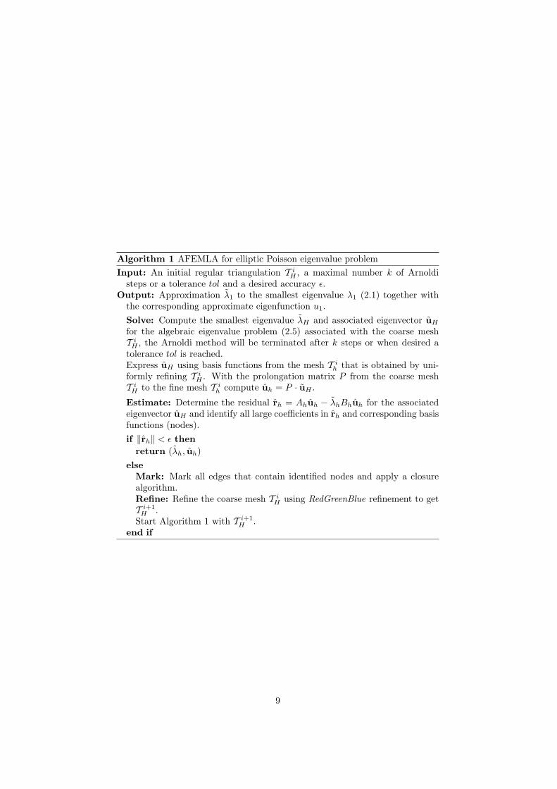
Algorithm 1 AFEMLA for elliptic Poisson eigenvalue problemInput: An initial regular triangulation T i

H , a maximal number k of Arnoldisteps or a tolerance tol and a desired accuracy ε.

Output: Approximation λ1 to the smallest eigenvalue λ1 (2.1) together withthe corresponding approximate eigenfunction u1.Solve: Compute the smallest eigenvalue λH and associated eigenvector uH

for the algebraic eigenvalue problem (2.5) associated with the coarse meshT i

H , the Arnoldi method will be terminated after k steps or when desired atolerance tol is reached.Express uH using basis functions from the mesh T i

h that is obtained by uni-formly refining T i

H . With the prolongation matrix P from the coarse meshT i

H to the fine mesh T ih compute uh = P · uH .

Estimate: Determine the residual rh = Ahuh − λhBhuh for the associatedeigenvector uH and identify all large coefficients in rh and corresponding basisfunctions (nodes).if ‖rh‖ < ε then

return (λh, uh)else

Mark: Mark all edges that contain identified nodes and apply a closurealgorithm.Refine: Refine the coarse mesh T i

H using RedGreenBlue refinement to getT i+1

H .Start Algorithm 1 with T i+1

H .end if

9

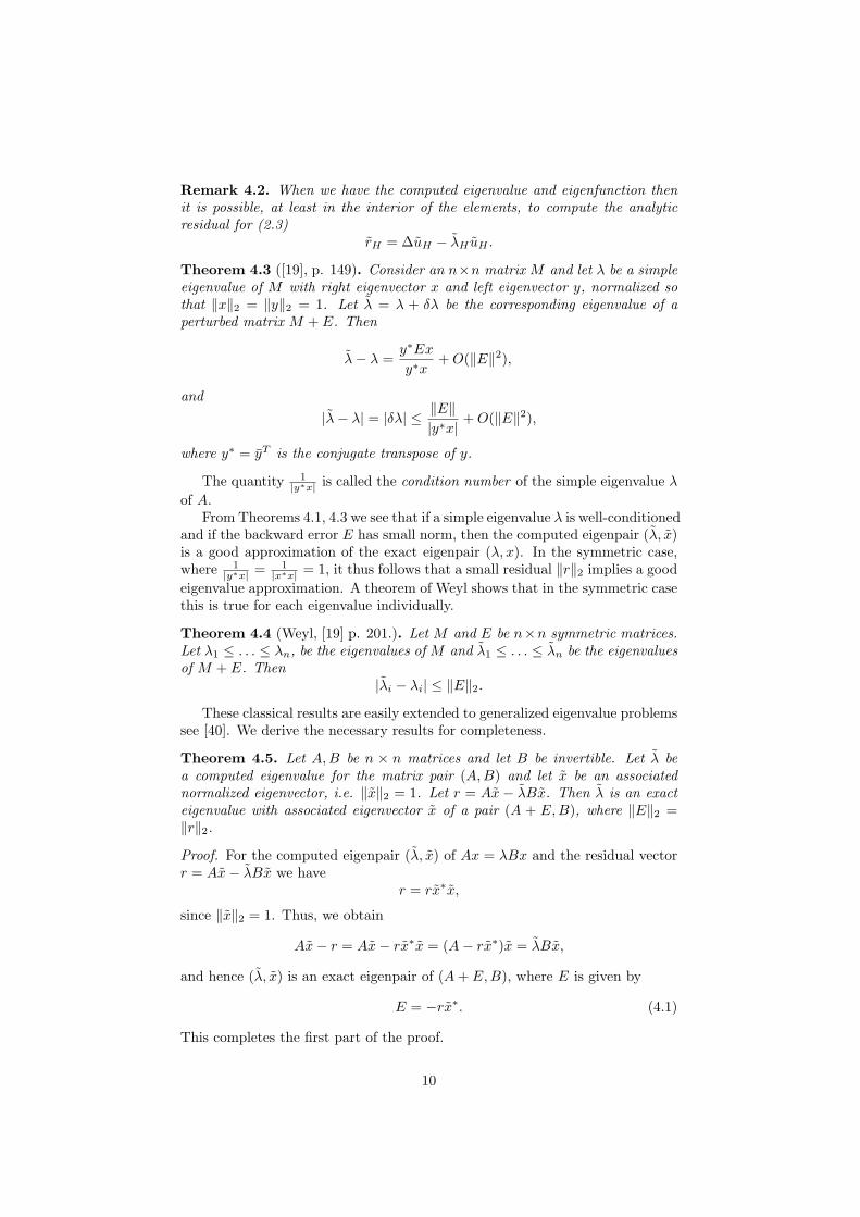
Remark 4.2. When we have the computed eigenvalue and eigenfunction thenit is possible, at least in the interior of the elements, to compute the analyticresidual for (2.3)

rH = ∆uH − λH uH .

Theorem 4.3 ([19], p. 149). Consider an n×n matrix M and let λ be a simpleeigenvalue of M with right eigenvector x and left eigenvector y, normalized sothat ‖x‖2 = ‖y‖2 = 1. Let λ = λ + δλ be the corresponding eigenvalue of aperturbed matrix M + E. Then

λ− λ =y∗Ex

y∗x+ O(‖E‖2),

and

|λ− λ| = |δλ| ≤ ‖E‖|y∗x|

+ O(‖E‖2),

where y∗ = yT is the conjugate transpose of y.

The quantity 1|y∗x| is called the condition number of the simple eigenvalue λ

of A.From Theorems 4.1, 4.3 we see that if a simple eigenvalue λ is well-conditioned

and if the backward error E has small norm, then the computed eigenpair (λ, x)is a good approximation of the exact eigenpair (λ, x). In the symmetric case,where 1

|y∗x| = 1|x∗x| = 1, it thus follows that a small residual ‖r‖2 implies a good

eigenvalue approximation. A theorem of Weyl shows that in the symmetric casethis is true for each eigenvalue individually.

Theorem 4.4 (Weyl, [19] p. 201.). Let M and E be n×n symmetric matrices.Let λ1 ≤ . . . ≤ λn, be the eigenvalues of M and λ1 ≤ . . . ≤ λn be the eigenvaluesof M + E. Then

|λi − λi| ≤ ‖E‖2.

These classical results are easily extended to generalized eigenvalue problemssee [40]. We derive the necessary results for completeness.

Theorem 4.5. Let A, B be n × n matrices and let B be invertible. Let λ bea computed eigenvalue for the matrix pair (A, B) and let x be an associatednormalized eigenvector, i.e. ‖x‖2 = 1. Let r = Ax− λBx. Then λ is an exacteigenvalue with associated eigenvector x of a pair (A + E,B), where ‖E‖2 =‖r‖2.

Proof. For the computed eigenpair (λ, x) of Ax = λBx and the residual vectorr = Ax− λBx we have

r = rx∗x,

since ‖x‖2 = 1. Thus, we obtain

Ax− r = Ax− rx∗x = (A− rx∗)x = λBx,

and hence (λ, x) is an exact eigenpair of (A + E,B), where E is given by

E = −rx∗. (4.1)

This completes the first part of the proof.

10

It follows from (4.1) that

‖E‖2 = ‖ − rx∗‖2 ≤ ‖r‖2‖x∗‖2 = ‖r‖2, (4.2)

but on the other hand we have that

‖r‖2 = ‖ − r‖2 = ‖ − rx∗x‖ = ‖Ex‖2 ≤ ‖E‖2‖x‖2 ≤ ‖E‖2. (4.3)

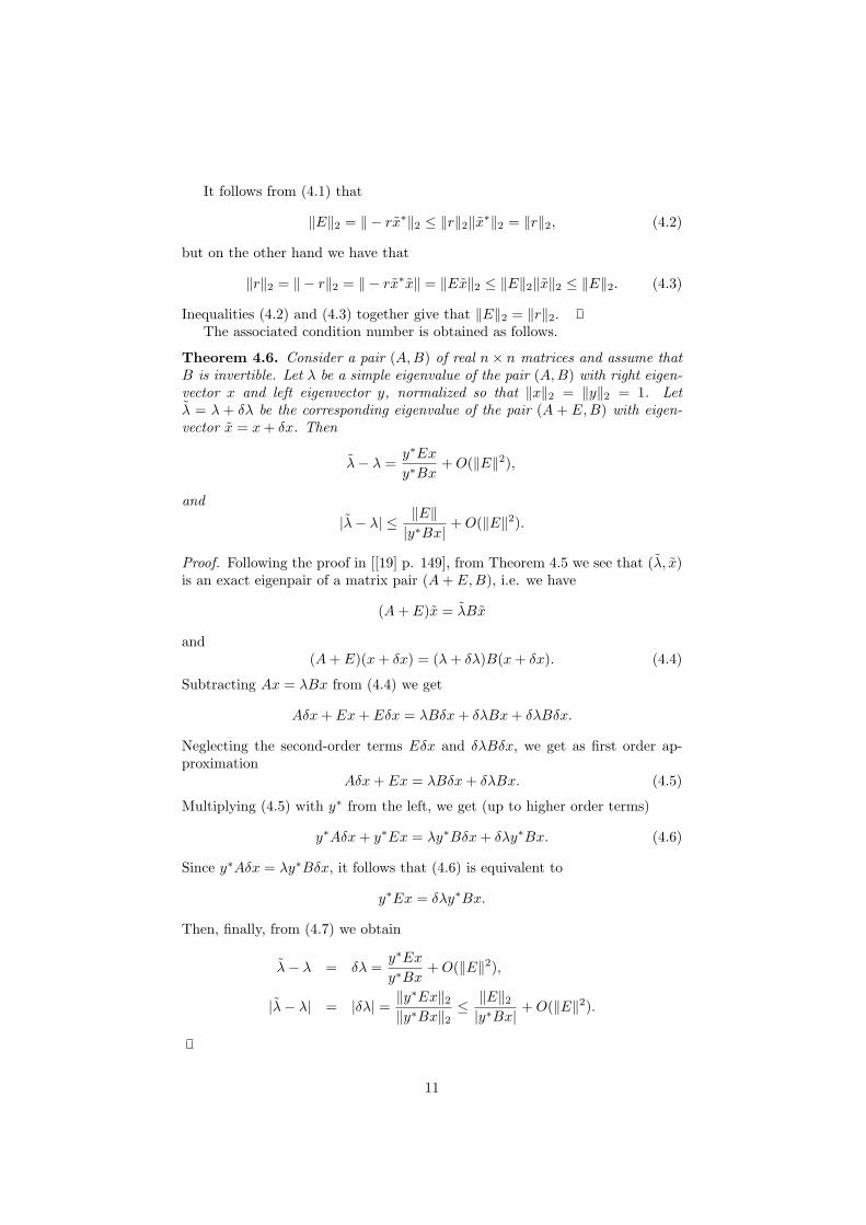
Inequalities (4.2) and (4.3) together give that ‖E‖2 = ‖r‖2.The associated condition number is obtained as follows.

Theorem 4.6. Consider a pair (A, B) of real n× n matrices and assume thatB is invertible. Let λ be a simple eigenvalue of the pair (A, B) with right eigen-vector x and left eigenvector y, normalized so that ‖x‖2 = ‖y‖2 = 1. Letλ = λ + δλ be the corresponding eigenvalue of the pair (A + E,B) with eigen-vector x = x + δx. Then

λ− λ =y∗Ex

y∗Bx+ O(‖E‖2),

and

|λ− λ| ≤ ‖E‖|y∗Bx|

+ O(‖E‖2).

Proof. Following the proof in [[19] p. 149], from Theorem 4.5 we see that (λ, x)is an exact eigenpair of a matrix pair (A + E,B), i.e. we have

(A + E)x = λBx

and(A + E)(x + δx) = (λ + δλ)B(x + δx). (4.4)

Subtracting Ax = λBx from (4.4) we get

Aδx + Ex + Eδx = λBδx + δλBx + δλBδx.

Neglecting the second-order terms Eδx and δλBδx, we get as first order ap-proximation

Aδx + Ex = λBδx + δλBx. (4.5)

Multiplying (4.5) with y∗ from the left, we get (up to higher order terms)

y∗Aδx + y∗Ex = λy∗Bδx + δλy∗Bx. (4.6)

Since y∗Aδx = λy∗Bδx, it follows that (4.6) is equivalent to

y∗Ex = δλy∗Bx.

Then, finally, from (4.7) we obtain

λ− λ = δλ =y∗Ex

y∗Bx+ O(‖E‖2),

|λ− λ| = |δλ| = ‖y∗Ex‖2‖y∗Bx‖2

≤ ‖E‖2|y∗Bx|

+ O(‖E‖2).

11

The quantity 1|y∗Bx| is again called the condition number of the simple eigen-

value λ. Since ‖E‖2 = ‖r‖2, for a small residual vector, good accuracy of theeigenvalue depends on this condition number.

In our special case of a symmetric generalized eigenvalue problem with pos-itive definite B, we thus obtain the following result.

Corollary 4.7. Let (λ, x) with ‖x‖2 = 1 be an exact eigenpair for a real sym-metric matrix pair (A, B) with positive definite matrix B and let (λ, x) be acorresponding computed eigenpair. Then

|λ− λ| ≤ ‖r‖2‖B−1‖2.

Proof. By Theorem 4.6 we have

|λ− λ| = ‖y∗Ex‖2|y∗Bx|

, ‖E‖2 = ‖r‖2.

Since in our case the left eigenvector is real and satisfies y = x, we obtain

1|y∗Bx|

≤ 1λmin(B)

= λmax(B−1) = ‖B−1‖2,

where λmin(B) is the minimal eigenvalue of B and λmax(B−1) is the maximaleigenvalue of B−1.

Hence with

|λ− λ| = ‖xT Ex‖2|xT Bx|

≤ ‖r‖2|xT Bx|

≤ ‖r‖2‖B−1‖2

the proof is complete.Using the previous theorems we will now prove some error bounds for the

discrete and continuous eigenvalues. We will denote by (λ, u) the exact pair ofeigenvalue and eigenfunction of (2.3), for diam = h, H, by (λdiam ,udiam ) theexact and by (λdiam , udiam ) computed eigenpairs for the discrete formulationwith respect to the finite space Vdiam . We denote by (λh, uh) the eigenpairobtained from the prolongation of the eigenvector uH to the finite space Vh.The corresponding residual vectors will be denoted by

rH = AH uH − λHBH uH , (4.7)rh = Ahuh − λhBhuh, (4.8)

rh = Ahuh − λhBhuh. (4.9)

We then have the following error bounds.

Theorem 4.8. Let (λH ,uH), (λh,uh) be the exact eigenvalues and associ-ated eigenvectors of the matrix pairs (AH , BH), (Ah, Bh), respectively, and let(λH , uH), (λh, uh) be corresponding computed eigenpairs. Let the eigenvectoruH , uh be normalized, i.e. ‖uH‖2 = ‖uh‖2 = 1. Then the following estimateshold.

|λH − λH | ≤ ‖rH‖2‖B−1H ‖2, (4.10)

|λh − λh| ≤ ‖rh‖2‖B−1h ‖2, (4.11)

|λh − λh| ≤ ‖rh‖2‖B−1h ‖2. (4.12)

12

Proof. With rH = AH uH − λHBH uH , by Theorem 4.7 we get

|λH − λH | ≤ ‖rH‖2‖B−1H ‖2.

Analogously, for rh = AH uh − λhBhuh we get

|λh − λh| ≤ ‖rh‖2‖B−1h ‖2.

The last inequality then follows from (3.1) and the definition of rh = Ahuh −λhBhuh.

It should be noted that in our algorithm we do not compute the fine grideigenpair (λh, uh). For this reason, the fine grid residual ‖rh‖2 is not available.Instead we use (λh, uh) as its approximation and have the following bounds.

Theorem 4.9. Let (λH , uH) be a computed eigenpair of the matrix pair (AH , BH)and let (λh, uh) be the computed eigenpair obtained by the prolongation (with theprolongation matrix P ) of uH to the fine space Vh as defined in (3.1). Assumethat these vectors are normalized, i.e. ‖uH‖2 = ‖uh‖2 = 1. Then

|λH − λh| ≤‖rH‖2 + ‖PT ‖2‖rh‖2

‖PT Bhuh‖2. (4.13)

Proof. Following Theorem 4.5, the eigenpairs (λH , uh), (λh, uh) are exact eigen-pairs of the eigenvalue problems

(AH + EH)uH = λHBH uH , (4.14)

(Ah + Eh)uh = λhBhuh, (4.15)

respectively.Using the relation between the coarse and the fine mesh, i.e. that

PT AhP = AH , PT BhP = BH ,

it follows that (4.14) is equivalent to

(PT AhP + EH)uH = λH(PT BhP )uH . (4.16)

Multiplying (4.15) from the left by PT gives

PT Ahuh + PT Ehuh = λhPT Bhuh. (4.17)

Using the fact that P uH = uh, we can rewrite (4.16) as

PT AhP uH + EH uH = λHPT BhP uH . (4.18)

Subtracting (4.17) from (4.18) we then get

(λH − λh)(PT Bhuh) = PT Ahuh + EH uH − PT Ahuh − PT Ehuh

and, applying the triangle inequality, finally

|λH − λh| =‖EH uH − PT Ehuh‖2

‖PT Bhuh‖2≤ ‖EH uH‖2 + ‖PT Ehuh‖2

‖PT Bhuh‖2

≤ ‖EH‖2‖uH‖2 + ‖PT Eh‖2‖uh‖2‖PT Bhuh‖2

=‖EH‖2 + ‖PT Eh‖2

‖PT Bhuh‖2

≤ ‖EH‖2 + ‖PT ‖2‖Eh‖2‖PT Bhuh‖2

=‖rH‖2 + ‖PT ‖2‖rh‖2

‖PT Bhuh‖2.

13

Having obtained an estimate between the computed eigenvalue on the coarsegrid and the prolongated eigenvalue on the fine mesh we next obtain a com-parison between the exact eigenvalue on the coarse grid and the prolongatedeigenvalue.

Theorem 4.10. Let (λH ,uH) be the exact eigenpair of the matrix pair (AH , BH)and let (λh, uh) be the eigenpair obtained by the prolongation (3.1) of uH to thefine space Vh. Then the following bound holds.

|λH − λh| ≤ ‖rH‖2‖B−1H ‖2 +

‖rH‖2 + ‖PT ‖2‖rh‖2‖PT Bhuh‖2

.

Proof. Using the triangle inequality we get

|λH − λh| = |λH − λH + λH − λh| ≤ |λH − λH |+ |λH − λh|.

Inserting the bounds (4.10) and (4.13) we get

|λH − λh| ≤ ‖rH‖2‖B−1H ‖2 +

‖rH‖2 + ‖PT ‖2‖rh‖2‖PT Bhuh‖2

.

Applying again the triangle inequality

|λH − λh| = |λH − λh + λh − λh| ≤ |λH − λh|+ |λh − λh|

we get an error estimate between the exact fine and course grid eigenvalue

|λH − λh| ≤ |rH‖2‖B−1H ‖2 +

‖rH‖2 + ‖PT ‖2‖rh‖2‖PT Bhuh‖2

+ ‖rh‖2‖B−1h ‖2 (4.19)

and between the exact fine grid and computed coarse grid eigenvalues.

|λh − λH | = |λh − λh + λh = λH | ≤ |λh − λh|+ |λh − λH |,

|λh − λH | ≤ ‖rh‖2‖B−1h ‖2 +

‖rH‖2 + ‖PT ‖2‖rh‖2‖PT Bhuh‖2

.

Combining these bounds and using the triangle inequality in different wayswe obtain the following further bounds.

Theorem 4.11. Let (λH ,uH), (λh,uh) be the exact and let (λH , uH), (λh, uh)be the computed eigenpairs of the matrix pair (AH , BH), (Ah, Bh), respectively.Let furthermore (λh, uh) be the eigenpair obtained by the prolongation of uH tothe fine space Vh defined in (3.1). Then the following bound holds.

|λh − λh| ≤ ‖rh‖2‖B−1h ‖2 + ‖rh‖2‖B−1

h ‖2,

|λH − λh| ≤ ‖rH‖2 + ‖PT ‖2‖rh‖2‖PT Bhuh‖2

+ ‖rh‖2‖B−1h ‖2 + ‖rh‖2‖B−1

h ‖2,

|λH − λh| ≤ ‖rH‖2‖B−1H ‖2 +

‖rH‖2 + ‖PT ‖2‖rh‖2‖PT Bhuh‖2

+ ‖rh‖2‖B−1h ‖2

+ ‖rh‖2‖B−1h ‖2.

14

Proof. The proof follows by combing the previous bounds and using the triangleinequality.

Theorems 4.8 - 4.11 present error bounds with respect to the exact andcomputed eigenvalues for the discretized algebraic problems. Some of thesebounds are computable but some have only theoretical meaning. Since in factwe are interested in errors between the eigenvalues of the continuous problemand those of the discrete problem, we would like to find computable boundsbased on residual vectors. Since we were able to transform residual errors tobackward errors it follows that for well-conditioned eigenvalues we can expectthat small residuals will imply good accuracy of its approximations obtained byiterative solvers.

In order to relate the continuous and discrete eigenvalues we will use theso called saturation assumption, namely we will assume that the approximationof the eigenvalue computed on the fine space Vh is better than the approxima-tion on the coarse space VH . In practice this assumption is equivalent to theconvergence of the AFEM procedure.

Theorem 4.12 ([37]). Let λ be an exact eigenvalue of (2.3). Let λH , λh be thecorresponding exact eigenvalues of the discretized problems on spaces VH , Vh,respectively. Then the saturation assumption

λh − λ ≤ β(λH − λ), (4.20)

with a positive β < 1, is equivalent to

λH − λ ≤ 11− β

(λH − λh). (4.21)

Remark 4.13. Since for the symmetric eigenvalue problem the Courant-Fischerminmax theorem holds, the exact eigenvalue λ of the PDE eigenvalue problemand the eigenvalues λH , λh of the discretized problems satisfy the inequality

λ ≤ λh ≤ λH .

Thus, the inequalities (4.20) and (4.21) are equivalent to |λh − λ| ≤ β(λH − λ)and |λH − λ| ≤ 1

1−β (λH − λh), respectively.

Based on the saturation assumption and the estimates between the differentand computed eigenvalues for the discretized eigenvalue problems we then obtainthe following bounds.

Theorem 4.14. Let λ be an exact eigenvalue of (2.3) and let u be the cor-responding eigenfunction. Let λH be the corresponding exact eigenvalue of thediscretized generalized eigenvalue problem (AH , BH), and let uH be defined asin (3.1). Then with residuals rH , rh as defined in (4.7), (4.9) we have

|λH − λ| ≤ 11− β

(‖rH‖2‖B−1

H ‖2 +‖rH‖2 + ‖PT ‖2‖rh‖2

‖PT Bhuh‖2+ ‖rh‖2‖B−1

h ‖2)

.

Proof. Under the saturation assumption it follows from Theorem 4.12 that

|λH − λ| ≤ 11− β

(λH − λh).

15

From (4.19) it follows that

|λH − λh| ≤ ‖rH‖2‖B−1H ‖2 +

‖rH‖2 + ‖PT ‖2‖rh‖2‖PT Bhuh‖2

+ ‖rh‖2‖B−1h ‖2

and thus

|λH − λ| ≤ 11− β

(‖rH‖2‖B−1

H ‖2 +‖rH‖2 + ‖PT ‖2‖rh‖2

‖PT Bhuh‖2+ ‖rh‖2‖B−1

h ‖2)

.

Theorem 4.15. Let λ be an exact eigenvalue of (2.3), let λh be the correspond-ing exact fine grid eigenvalue and let uH be defined as in (3.1). Then withresiduals rH , rh defined as in (4.7), (4.9) we have

|λh−λ| ≤ (1− 11− β

)(‖rH‖2‖B−1

H ‖2 +‖rH‖2 + ‖PT ‖2‖rh‖2

‖PT Bhuh‖2+ ‖rh‖2‖B−1

h ‖2)

.

Proof. Under the saturation assumption it follows from Theorem 4.12 that

|λh − λ| ≤ λh − λH +1

1− β(λH − λh) = (1− 1

1− β)(λh − λH).

From (4.19) we have that

|λH − λh| ≤ ‖rH‖2‖B−1H ‖2 +

‖rH‖2 + ‖PT ‖2‖rh‖2‖PT Bhuh‖2

+ ‖rh‖2‖B−1h ‖2

and hence

|λh−λ| ≤ (1− 11− β

)(‖rH‖2‖B−1

H ‖2 +‖rH‖2 + ‖PT ‖2‖rh‖2

‖PT Bhuh‖2+ ‖rh‖2‖B−1

h ‖2)

.

Using the previous estimates we can also obtain a bound between the com-puted eigenvalue on the coarse mesh and the corresponding eigenvalues of theoriginal PDE eigenvalue problem.

Theorem 4.16. Let λ be an exact eigenvalue of (2.3) and let λH be the com-puted coarse grid eigenvalue and let uh be defined as in (3.1). Then with resid-uals rH , rh defined as in (4.7), (4.9), we have

|λH − λ| ≤ 11− β

(‖rH‖2‖B−1

H ‖2 +‖rH‖2 + ‖PT ‖2‖rh‖2

‖PT Bhuh‖2+ ‖rh‖2‖B−1

h ‖2)

+ ‖rH‖2‖B−1H ‖2.

Proof. From (4.7) we know that

|λH − λH | ≤ ‖rH‖2‖B−1H ‖2

and from Theorem 4.14 we have that

|λH − λ| ≤ 11− β

(‖rH‖2‖B−1

H ‖2 +‖rH‖2 + ‖PT ‖2‖rh‖2

‖PT Bhuh‖2+ ‖rh‖2‖B−1

h ‖2)

.

16

Hence,

|λH − λ| ≤ 11− β

(‖rH‖2‖B−1

H ‖2 +‖rH‖2 + ‖PT ‖2‖rh‖2

‖PT Bhuh‖2+ ‖rh‖2‖B−1

h ‖2)

+ ‖rH‖2‖B−1H ‖2.

Theorem 4.17. Let λ be an exact eigenvalue of (2.3) and let uH be the com-puted coarse grid eigenvector. Furthermore, let (λh, uh) be the correspondingeigenpair obtained by the prolongation of uH to the fine space Vh defined as in(3.1). Then with residuals rH , rh as defined in (4.7), (4.9) we have

|λh − λ| ≤ ‖rH‖2‖B−1H ‖2 +

‖rH‖2 + ‖PT ‖2‖rh‖2‖PT Bhuh‖2

+1

1− β

(‖rH‖2‖B−1

H ‖2 +‖rH‖2 + ‖PT ‖2‖rh‖2

‖PT Bhuh‖2+ ‖rh‖2‖B−1

h ‖2)

.

Proof. From Theorem 4.10 it follows that

|λH − λh| ≤ ‖rH‖2‖B−1H ‖2 +

‖rH‖2 + ‖PT ‖2‖rh‖2‖PT Bhuh‖2

and from Theorem 4.14 we have that

|λH − λ| ≤ 11− β

(‖rH‖2‖B−1

H ‖2 +‖rH‖2 + ‖PT ‖2‖rh‖2

‖PT Bhuh‖2+ ‖rh‖2‖B−1

h ‖2)

and hence,

|λh − λ| ≤ ‖rH‖2‖B−1H ‖2 +

‖rH‖2 + ‖PT ‖2‖rh‖2‖PT Bhuh‖2

+1

1− β

(‖rH‖2‖B−1

H ‖2 +‖rH‖2 + ‖PT ‖2‖rh‖2

‖PT Bhuh‖2+ ‖rh‖2‖B−1

h ‖2)

.

Theorem 4.18. Let λ be an exact eigenvalue of (2.3), λh the computed finegrid eigenvalue. Then with residuals rH , rh, rh as defined in (4.7), (4.8), (4.9)we have

|λh − λ| ≤ (1− 11− β

)(‖rH‖2‖B−1

H ‖2 +‖rH‖2 + ‖PT ‖2‖rh‖2

‖PT Bhuh‖2+ ‖rh‖2‖B−1

h ‖2)

+ ‖rh‖2‖B−1h ‖2

Proof. From Theorem 4.8 it follows that

|λh − λh| ≤ ‖rh‖2‖B−1h ‖2

and from Theorem 4.15 we have that

|λh−λ| ≤ (1− 11− β

)(‖rH‖2‖B−1

H ‖2 +‖rH‖2 + ‖PT ‖2‖rh‖2

‖PT Bhuh‖2+ ‖rh‖2‖B−1

h ‖2)

17

and hence

|λh − λ| ≤ (1− 11− β

)(‖rH‖2‖B−1

H ‖2 +‖rH‖2 + ‖PT ‖2‖rh‖2

‖PT Bhuh‖2+ ‖rh‖2‖B−1

h ‖2)

+ ‖rh‖2‖B−1h ‖2.

In summary, we have obtained bounds between the exact eigenvalues andeigenvalue approximations. We can immediately notice, that all bounds exceptfor the last bound in Theorem 4.18 are fully computable. As a matter of fact thelast bound has only theoretical value because we do not want to compute theresidual rh on the fine mesh. But it follows from all these bounds, that underthe saturation assumption, and if we consider problems with well-conditionedeigenvalues, then the information about a small residual vector is equivalent tothe good accuracy of the computed eigenvalues.

5 Numerical experiments

In this section, we present some numerical results that illustrate our algorithm.The numerical tests where partially realized with help of the finite elementprogram openFFW [13] published under GNU General Public License v.3. Weconsider the eigenvalue problem

∆u = λu in Ω, (5.1)u = 0 on ∂Ω.

on different domains Ω.

5.1 L-shape domain

Let us consider the eigenvalue problem (5.1) with L-shape domain Ω = [−1, 1]×[0, 1] ∪ [−1, 0]× [−1, 0]. An approximation of the smallest eigenvalue was givenin [43], where the authors obtained that

λ1 ≈ 9.639723844.

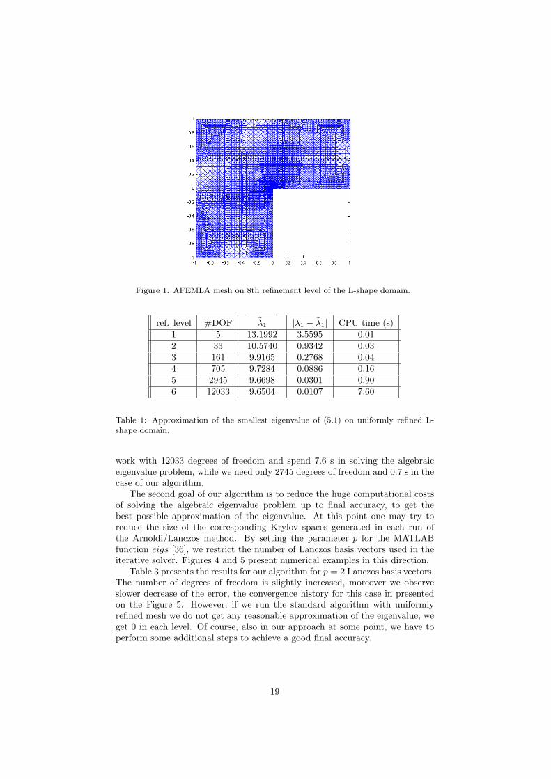
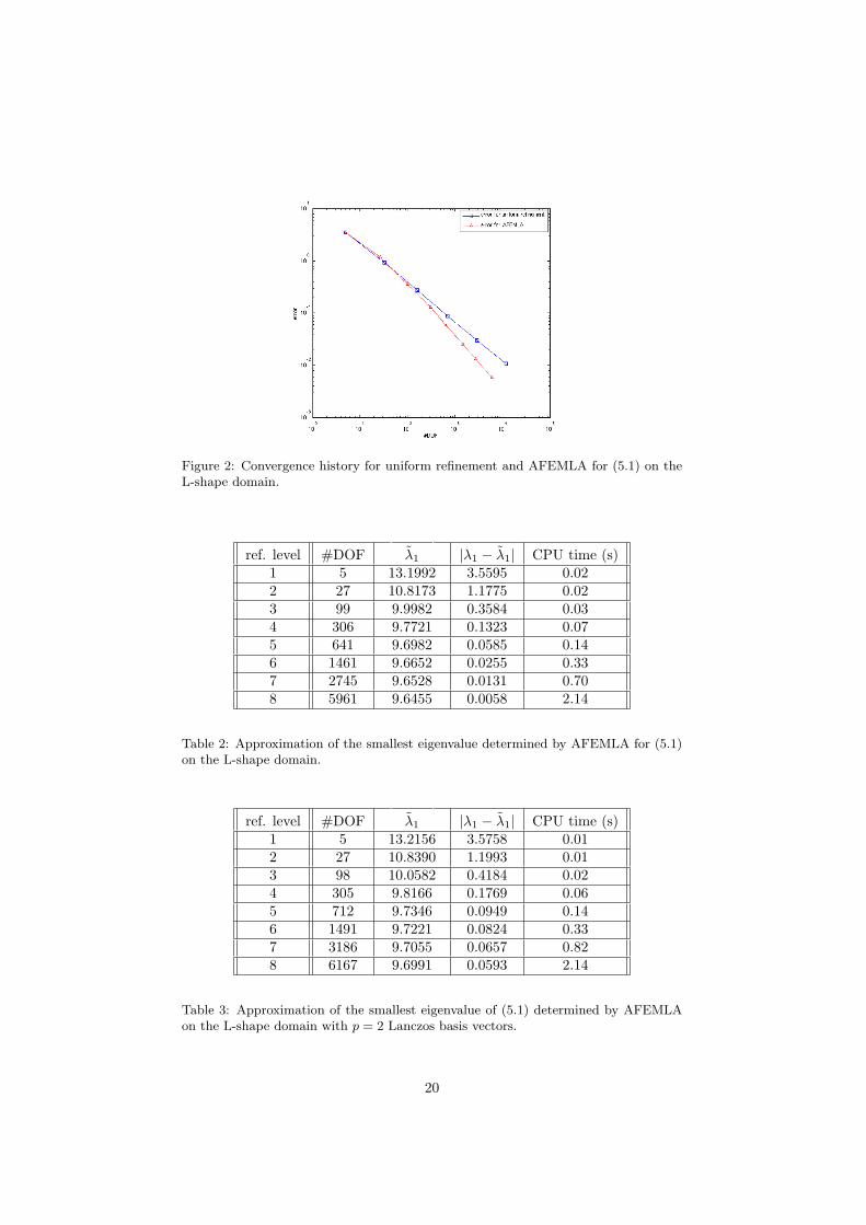
Figure 1 shows the adaptively refined mesh on the 8-th level of refinement.We note that the mesh constructed by our algorithm contains more elementsaround the singularity. Additionally the convergence history is given in Figure 2,namely the log-log plot of the approximation error versus the number of degreesof freedom. This error is |λ − λ|, where the discrete eigenvalue problem issolved using the Arnoldi/Lanczos method, namely the MATLAB function eigs[36]. The squares show the approximation error based on the computationon the uniformly refined grid, while the triangles illustrate the approximationfor our residual based refined grid. This shows that with our algorithm wemay reach the same accuracy of the computed eigenvalue with fewer degrees offreedom. Tables 1 and 2 present the convergence history data for both strategies.Comparing the last columns of both tables, where we present the MATLAB CPUtimes of running the iterative algebraic eigenvalue solver for both algorithms,we notice that to reach the accuracy 10−2 for the first algorithm we have to

18

Figure 1: AFEMLA mesh on 8th refinement level of the L-shape domain.

ref. level #DOF A λ1 A |λ1 − λ1| CPU time (s)1 5 13.1992 3.5595 0.012 33 10.5740 0.9342 0.033 161 9.9165 0.2768 0.044 705 9.7284 0.0886 0.165 2945 9.6698 0.0301 0.906 12033 9.6504 0.0107 7.60

Table 1: Approximation of the smallest eigenvalue of (5.1) on uniformly refined L-shape domain.

work with 12033 degrees of freedom and spend 7.6 s in solving the algebraiceigenvalue problem, while we need only 2745 degrees of freedom and 0.7 s in thecase of our algorithm.

The second goal of our algorithm is to reduce the huge computational costsof solving the algebraic eigenvalue problem up to final accuracy, to get thebest possible approximation of the eigenvalue. At this point one may try toreduce the size of the corresponding Krylov spaces generated in each run ofthe Arnoldi/Lanczos method. By setting the parameter p for the MATLABfunction eigs [36], we restrict the number of Lanczos basis vectors used in theiterative solver. Figures 4 and 5 present numerical examples in this direction.

Table 3 presents the results for our algorithm for p = 2 Lanczos basis vectors.The number of degrees of freedom is slightly increased, moreover we observeslower decrease of the error, the convergence history for this case in presentedon the Figure 5. However, if we run the standard algorithm with uniformlyrefined mesh we do not get any reasonable approximation of the eigenvalue, weget 0 in each level. Of course, also in our approach at some point, we have toperform some additional steps to achieve a good final accuracy.

19

Figure 2: Convergence history for uniform refinement and AFEMLA for (5.1) on theL-shape domain.

ref. level #DOF A λ1 A |λ1 − λ1| CPU time (s)1 5 13.1992 3.5595 0.022 27 10.8173 1.1775 0.023 99 9.9982 0.3584 0.034 306 9.7721 0.1323 0.075 641 9.6982 0.0585 0.146 1461 9.6652 0.0255 0.337 2745 9.6528 0.0131 0.708 5961 9.6455 0.0058 2.14

Table 2: Approximation of the smallest eigenvalue determined by AFEMLA for (5.1)on the L-shape domain.

ref. level #DOF A λ1 A |λ1 − λ1| CPU time (s)1 5 13.2156 3.5758 0.012 27 10.8390 1.1993 0.013 98 10.0582 0.4184 0.024 305 9.8166 0.1769 0.065 712 9.7346 0.0949 0.146 1491 9.7221 0.0824 0.337 3186 9.7055 0.0657 0.828 6167 9.6991 0.0593 2.14

Table 3: Approximation of the smallest eigenvalue of (5.1) determined by AFEMLAon the L-shape domain with p = 2 Lanczos basis vectors.

20

Figure 3: The eigenfunction corresponding to the eigenvalue λ = 9.6455 on the L-shapedomain.

ref. level 1 2 3 4 5 6#DOF 5 33 161 705 2945 12033mesh T1 13.1992 10.5740 9.9165 9.7284 9.6698 9.6504mesh T2 13.1992 10.5930 9.9261 9.7315 9.6707 9.6507

Table 4: Approximation of the smallest eigenvalue of (5.1) on the uniformly refinedgrids with initial mesh T1 and T2.

5.2 Dependence on the layout of the initial grid

In Figure 6 and 7 we present two very similar initial meshes, however runningthe standard algorithm with uniform refinement on these meshes at each stepprovides interesting results. Analyzing results summarized in Table 4 we observea faster convergence of the algorithm with initial mesh T1, with the same numberof grid points generated in each point. After some steps we get the errors of thesame order but we observe slightly better behavior for the initial mesh T1. Thisresult shows, that not only the number of degrees of freedom plays a role in theconvergence of the AFEM, but also the distribution over the domain.

5.3 More complicated domains

Let us consider the eigenvalue problem (5.1) with domain Ω as in Figure 8. Sincein this case we do not know a priori any good approximation of the smallesteigenvalue, for comparison we will use the values obtained by exact procedurerun on the uniformly refined grid in each step.

Comparing the values listed in Table 5 and 6 we notice that to obtain theapproximation λ ≈ 11.97 using uniformly refined grids we need around 69825degrees of freedom while in our algorithm we work with 9584 degrees of freedom.Moreover, when we look at the run time for the iterative procedure, for theuniform algorithm we need around 788 s, while in our case we only need 4.6 s.

21

Figure 4: AFEMLA mesh on 8th refinement level of the L-shape domain with p = 2Lanczos basis vectors.

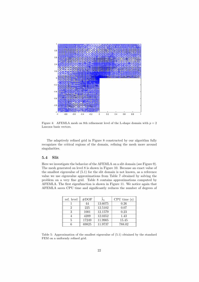
The adaptively refined grid in Figure 8 constructed by our algorithm fullyrecognizes the critical regions of the domain, refining the mesh more aroundsingularities.

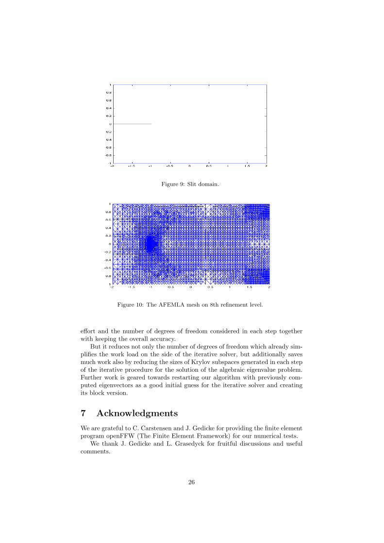
5.4 Slit

Here we investigate the behavior of the AFEMLA on a slit domain (see Figure 9).The mesh generated on level 8 is shown in Figure 10. Because an exact value ofthe smallest eigenvalue of (5.1) for the slit domain is not known, as a referencevalue we use eigenvalue approximations from Table 7 obtained by solving theproblem on a very fine grid. Table 8 contains approximations computed byAFEMLA. The first eigenfunction is shown in Figure 11. We notice again thatAFEMLA saves CPU time and significantly reduces the number of degrees of

ref. level #DOF A λ1 A CPU time (s)1 44 13.6075 0.262 225 12.5102 0.073 1001 12.1579 0.234 4209 12.0352 1.435 17249 11.9905 15.456 69825 11.9737 788.02

Table 5: Approximation of the smallest eigenvalue of (5.1) obtained by the standardFEM on a uniformly refined grid.

22

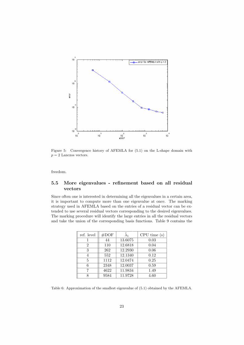
Figure 5: Convergence history of AFEMLA for (5.1) on the L-shape domain withp = 2 Lanczos vectors.

freedom.

5.5 More eigenvalues - refinement based on all residualvectors

Since often one is interested in determining all the eigenvalues in a certain area,it is important to compute more than one eigenvalue at once. The markingstrategy used in AFEMLA based on the entries of a residual vector can be ex-tended to use several residual vectors corresponding to the desired eigenvalues.The marking procedure will identify the large entries in all the residual vectorsand take the union of the corresponding basis functions. Table 9 contains the

ref. level #DOF A λ1 A CPU time (s)1 44 13.6075 0.032 110 12.6818 0.043 262 12.2930 0.064 552 12.1340 0.125 1112 12.0474 0.256 2348 12.0037 0.597 4622 11.9834 1.498 9584 11.9728 4.60

Table 6: Approximation of the smallest eigenvalue of (5.1) obtained by the AFEMLA.

23

ref. level #DOF A λ1 A CPU time (s)1 2 5.1429 0.292 19 3.8704 0.043 101 3.5444 0.044 457 3.4538 0.115 1937 3.4253 0.526 7969 3.4150 3.997 32321 3.4109 120.53

Table 7: Approximation of the smallest eigenvalue of (5.1) obtained by the standardFEM on a uniformly refined slit domain.

ref. level #DOF A λ1 A CPU time (s)1 2 5.1429 0.022 12 3.9949 0.013 46 3.6020 0.024 148 3.4895 0.045 354 3.4462 0.096 723 3.4271 0.157 1496 3.4173 0.348 3030 3.4125 0.81

Table 8: Approximation of the smallest eigenvalue of (5.1) obtained by the AFEMLAon the slit domain.

24

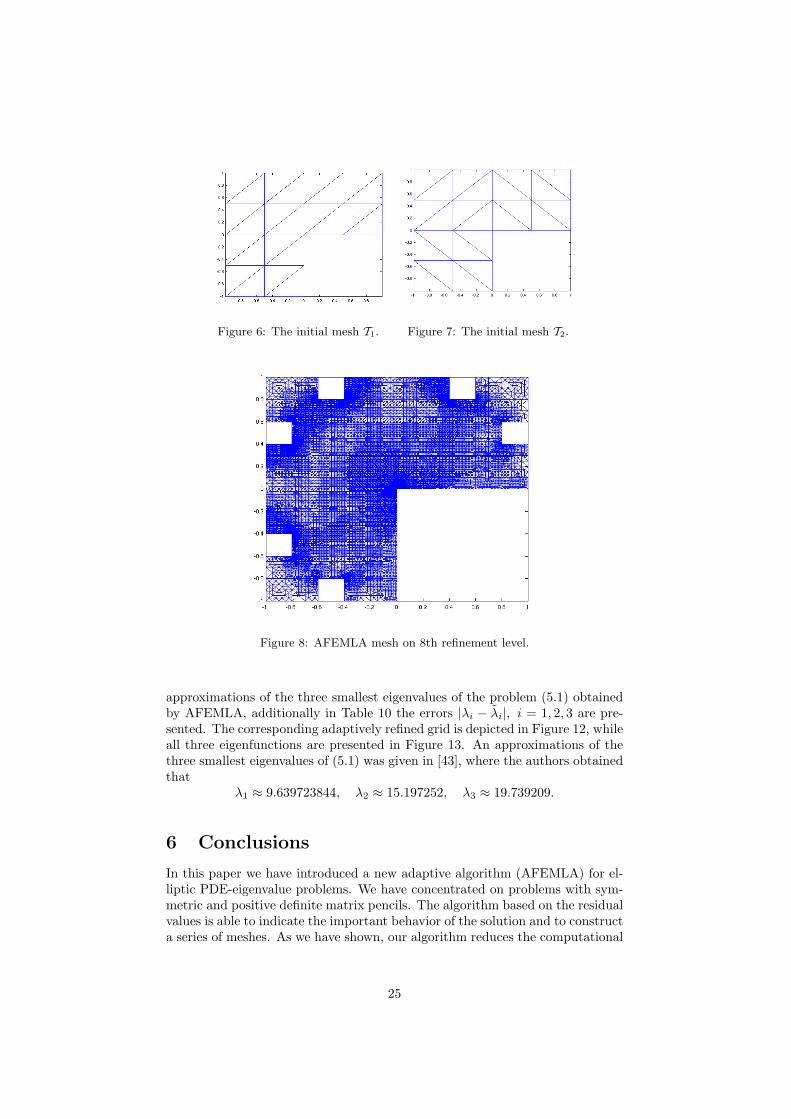
Figure 6: The initial mesh T1. Figure 7: The initial mesh T2.

Figure 8: AFEMLA mesh on 8th refinement level.

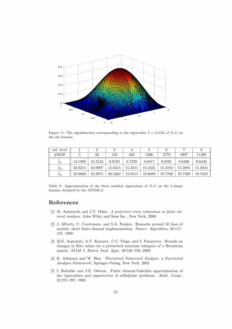
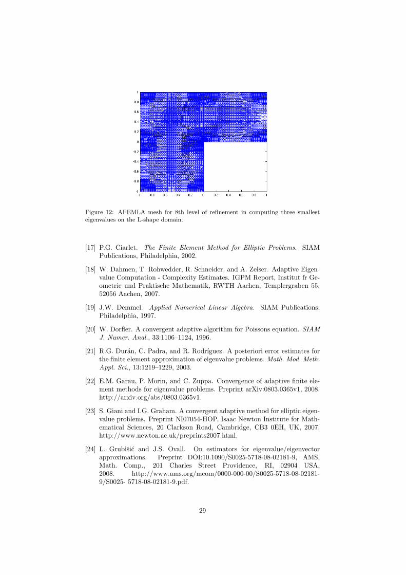
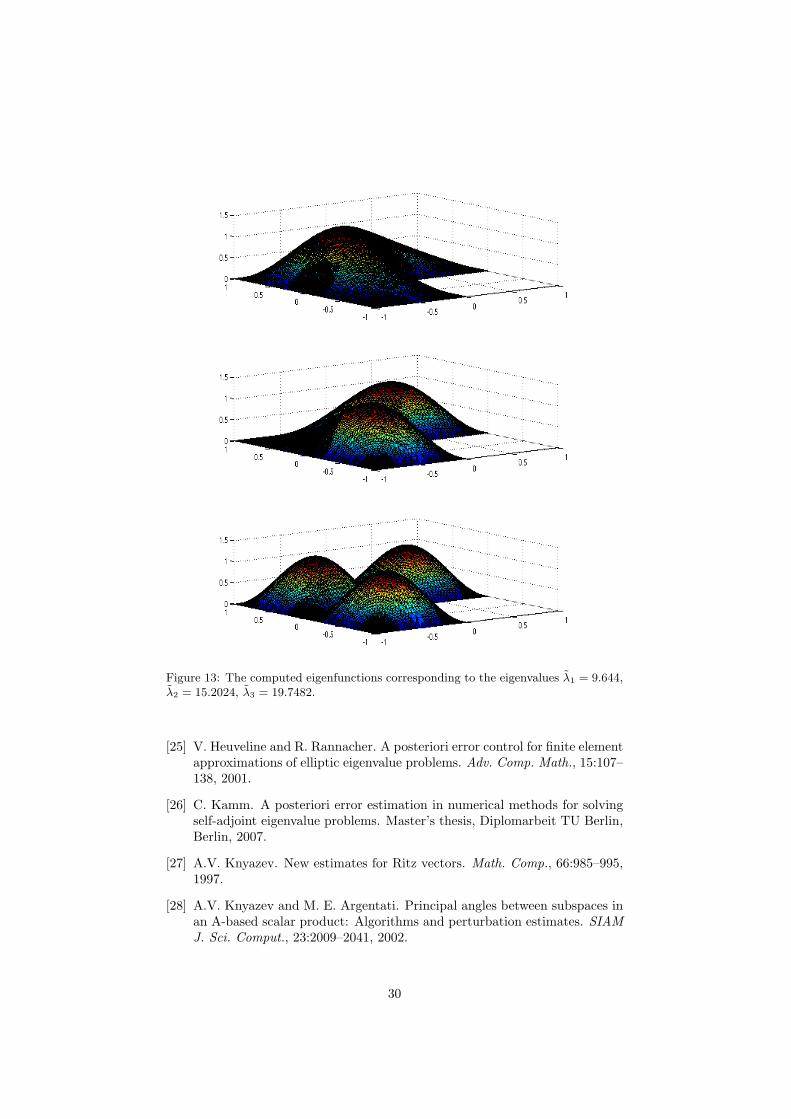
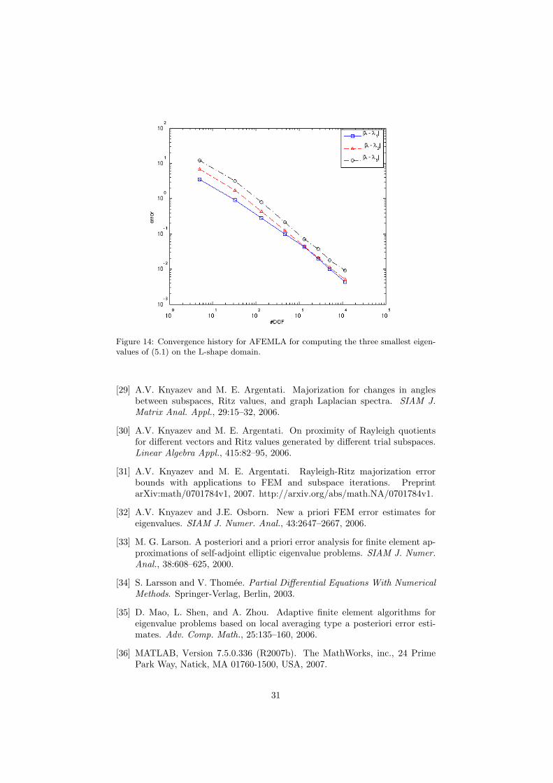
approximations of the three smallest eigenvalues of the problem (5.1) obtainedby AFEMLA, additionally in Table 10 the errors |λi − λi|, i = 1, 2, 3 are pre-sented. The corresponding adaptively refined grid is depicted in Figure 12, whileall three eigenfunctions are presented in Figure 13. An approximations of thethree smallest eigenvalues of (5.1) was given in [43], where the authors obtainedthat

λ1 ≈ 9.639723844, λ2 ≈ 15.197252, λ3 ≈ 19.739209.

6 Conclusions

In this paper we have introduced a new adaptive algorithm (AFEMLA) for el-liptic PDE-eigenvalue problems. We have concentrated on problems with sym-metric and positive definite matrix pencils. The algorithm based on the residualvalues is able to indicate the important behavior of the solution and to constructa series of meshes. As we have shown, our algorithm reduces the computational

25

Figure 9: Slit domain.

Figure 10: The AFEMLA mesh on 8th refinement level.

effort and the number of degrees of freedom considered in each step togetherwith keeping the overall accuracy.

But it reduces not only the number of degrees of freedom which already sim-plifies the work load on the side of the iterative solver, but additionally savesmuch work also by reducing the sizes of Krylov subspaces generated in each stepof the iterative procedure for the solution of the algebraic eigenvalue problem.Further work is geared towards restarting our algorithm with previously com-puted eigenvectors as a good initial guess for the iterative solver and creatingits block version.

7 Acknowledgments

We are grateful to C. Carstensen and J. Gedicke for providing the finite elementprogram openFFW (The Finite Element Framework) for our numerical tests.

We thank J. Gedicke and L. Grasedyck for fruitful discussions and usefulcomments.

26

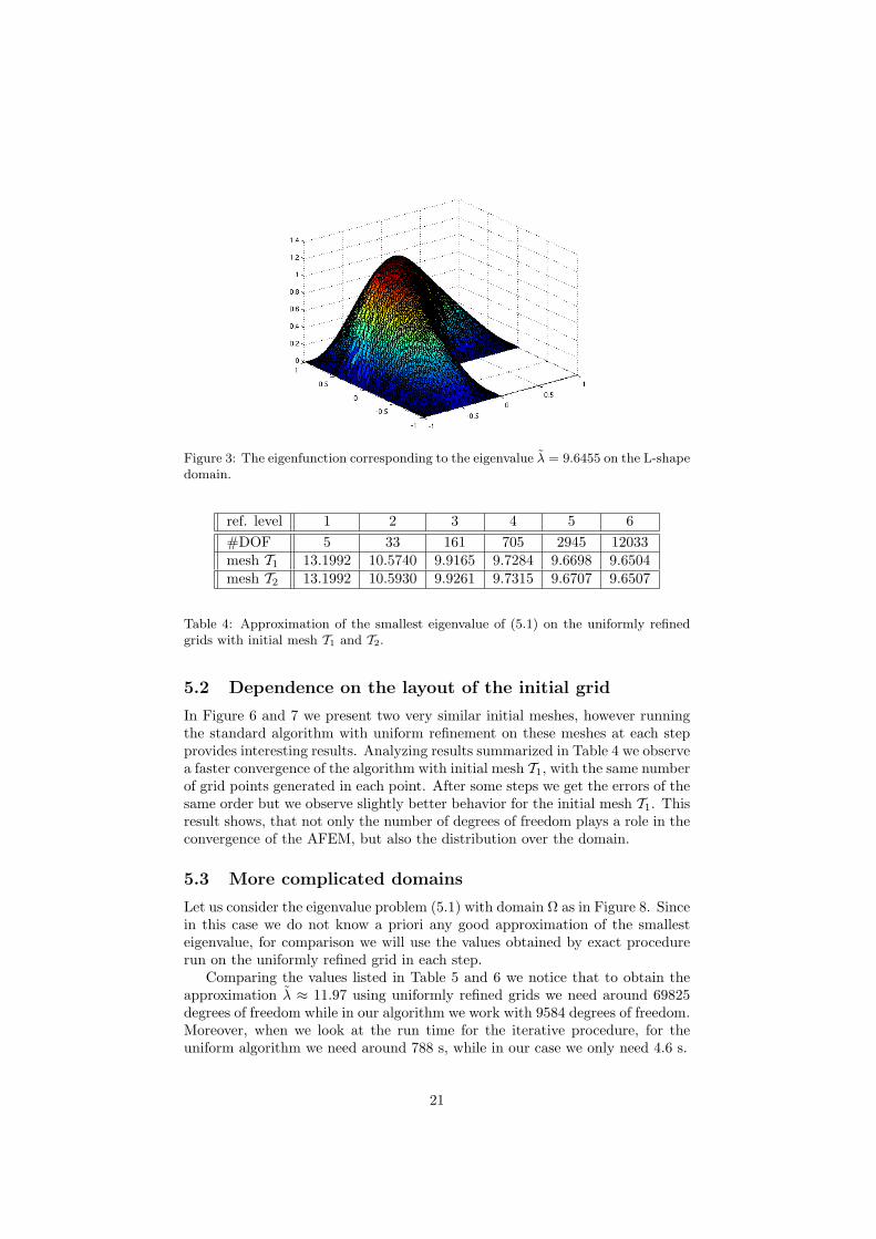
Figure 11: The eigenfunction corresponding to the eigenvalue λ = 3.4125 of (5.1) onthe slit domain.

ref. level 1 2 3 4 5 6 7 8#DOF 5 33 133 465 1306 2770 4997 11499

A λ1 A 13.1992 10.5542 9.9192 9.7376 9.6817 9.6591 9.6496 9.6440

A λ2 A 22.0215 16.9097 15.6315 15.3211 15.2421 15.2184 15.2085 15.2024

A λ3 A 32.0000 22.9075 20.5262 19.9515 19.8089 19.7760 19.7569 19.7482

Table 9: Approximation of the three smallest eigenvalues of (5.1) on the L-shapedomain obtained by the AFEMLA.

References

[1] M. Ainsworth and J.T. Oden. A posteriori error estimation in finite ele-ment analysis. John Wiley and Sons Inc., New York, 2000.

[2] J. Alberty, C. Carstensen, and S.A. Funken. Remarks around 50 lines ofmatlab: short finite element implementation. Numer. Algorithms, 20:117–137, 1999.

[3] M.E. Argentati, A.V. Knyazev, C.C. Paige, and I. Panayotov. Bounds onchanges in Ritz values for a perturbed invariant subspace of a Hermitianmatrix. SIAM J. Matrix Anal. Appl., 30:548–559, 2008.

[4] K. Atkinson and W. Han. Theoretical Numerical Analysis, a FunctionalAnalysis Framework. Springer-Verlag, New York, 2001.

[5] I. Babuska and J.E. Osborn. Finite element-Galerkin approximation ofthe eigenvalues and eigenvectors of selfadjoint problems. Math. Comp.,52:275–297, 1989.

27

ref. level 1 2 3 4 5 6 7 8

A |λ1 − λ1| A 3.5595 0.9144 0.2795 0.0979 0.0420 0.0194 0.0099 0.0043

A |λ2 − λ2| A 6.8242 1.7125 0.4342 0.1239 0.0448 0.0211 0...0112 0.0051

A |λ3 − λ3| A 12.2608 3.1683 0.7870 0.2123 0.0697 0.0367 0.0177 0.0090

Table 10: Errors corresponding to the three smallest eigenvalues of (5.1) on the L-shapedomain obtained by the AFEMLA.

ref. level 1 2 3 4 5 6 7 8CPU time (s) 0.0074 0.0281 0.0465 0.1131 0.3498 0.8469 1.8888 7.0342

Table 11: CPU time (s) for running the iterative algebraic eigenvalue solver.

[6] I. Babuska and J.E. Osborn. Eigenvalue problems. Handbook of NumericalAnalysis Vol. II. North-Holland, Amsterdam, 1991.

[7] Z. Bai, J. Demmel, J. Dongarra, A. Ruhe, and H. van der Vorst. Templatesfor the Solution of Algebraic Eigenvalue Problem. A Practical Guide. SIAMPublications, Philadelphia, 2000.

[8] R. E. Bank and R. K. Smith. A posteriori error estimates based on hierar-chical bases. SIAM J. Numer. Anal., 30:921–935, 1993.

[9] R. Becker and R. Rannacher. An optimal control approach to a posteriorierror estimation in finite element methods. Acta Numerica, 10:1–102, 2001.

[10] D. Braess. Finite elements. Cambridge University Press, New York, 2008.

[11] S.C. Brenner and C. Carstensen. Finite element methods. In E. Stein,R. de Borst, and T.J.R. Huges, editors, Encyclopedia of ComputationalMechanics, Vol. I, pages 73–114. John Wiley and Sons Inc., New York,2004.

[12] S.C. Brenner and L.R. Scott. The Mathematical Theory of Finite ElementMethods. Springer-Verlag, Berlin, 2008.

[13] A. Byfut, J. Gedicke, D. Gunther, J. Reininghaus, and S. Wiedemann.openFFW, The Finite Element Framework. GNU General Public Licensev.3.

[14] C. Carstensen. Some remarks on the history and future of averaging tech-niques in a posteriori finite element error analysis. Z. Angew. Math. Mech.,84:3–21, 2004.

[15] C. Carstensen and J. Gedicke. An oscillation-free adaptive FEM for sym-metric eigenvalue problems. Preprint 489, DFG Research Center Math-eon, Straße des 17. Juni 136, D-10623 Berlin, 2008.

[16] F. Chatelin. Spectral Approximation of Linear Operators. Academic Press,New York, 1983.

28

Figure 12: AFEMLA mesh for 8th level of refinement in computing three smallesteigenvalues on the L-shape domain.

[17] P.G. Ciarlet. The Finite Element Method for Elliptic Problems. SIAMPublications, Philadelphia, 2002.

[18] W. Dahmen, T. Rohwedder, R. Schneider, and A. Zeiser. Adaptive Eigen-value Computation - Complexity Estimates. IGPM Report, Institut fr Ge-ometrie und Praktische Mathematik, RWTH Aachen, Templergraben 55,52056 Aachen, 2007.

[19] J.W. Demmel. Applied Numerical Linear Algebra. SIAM Publications,Philadelphia, 1997.

[20] W. Dorfler. A convergent adaptive algorithm for Poissons equation. SIAMJ. Numer. Anal., 33:1106–1124, 1996.

[21] R.G. Duran, C. Padra, and R. Rodrıguez. A posteriori error estimates forthe finite element approximation of eigenvalue problems. Math. Mod. Meth.Appl. Sci., 13:1219–1229, 2003.

[22] E.M. Garau, P. Morin, and C. Zuppa. Convergence of adaptive finite ele-ment methods for eigenvalue problems. Preprint arXiv:0803.0365v1, 2008.http://arxiv.org/abs/0803.0365v1.

[23] S. Giani and I.G. Graham. A convergent adaptive method for elliptic eigen-value problems. Preprint NI07054-HOP, Isaac Newton Institute for Math-ematical Sciences, 20 Clarkson Road, Cambridge, CB3 0EH, UK, 2007.http://www.newton.ac.uk/preprints2007.html.

[24] L. Grubisic and J.S. Ovall. On estimators for eigenvalue/eigenvectorapproximations. Preprint DOI:10.1090/S0025-5718-08-02181-9, AMS,Math. Comp., 201 Charles Street Providence, RI, 02904 USA,2008. http://www.ams.org/mcom/0000-000-00/S0025-5718-08-02181-9/S0025- 5718-08-02181-9.pdf.

29

Figure 13: The computed eigenfunctions corresponding to the eigenvalues λ1 = 9.644,λ2 = 15.2024, λ3 = 19.7482.

[25] V. Heuveline and R. Rannacher. A posteriori error control for finite elementapproximations of elliptic eigenvalue problems. Adv. Comp. Math., 15:107–138, 2001.

[26] C. Kamm. A posteriori error estimation in numerical methods for solvingself-adjoint eigenvalue problems. Master’s thesis, Diplomarbeit TU Berlin,Berlin, 2007.

[27] A.V. Knyazev. New estimates for Ritz vectors. Math. Comp., 66:985–995,1997.

[28] A.V. Knyazev and M. E. Argentati. Principal angles between subspaces inan A-based scalar product: Algorithms and perturbation estimates. SIAMJ. Sci. Comput., 23:2009–2041, 2002.

30

Figure 14: Convergence history for AFEMLA for computing the three smallest eigen-values of (5.1) on the L-shape domain.

[29] A.V. Knyazev and M. E. Argentati. Majorization for changes in anglesbetween subspaces, Ritz values, and graph Laplacian spectra. SIAM J.Matrix Anal. Appl., 29:15–32, 2006.

[30] A.V. Knyazev and M. E. Argentati. On proximity of Rayleigh quotientsfor different vectors and Ritz values generated by different trial subspaces.Linear Algebra Appl., 415:82–95, 2006.

[31] A.V. Knyazev and M. E. Argentati. Rayleigh-Ritz majorization errorbounds with applications to FEM and subspace iterations. PreprintarXiv:math/0701784v1, 2007. http://arxiv.org/abs/math.NA/0701784v1.

[32] A.V. Knyazev and J.E. Osborn. New a priori FEM error estimates foreigenvalues. SIAM J. Numer. Anal., 43:2647–2667, 2006.

[33] M. G. Larson. A posteriori and a priori error analysis for finite element ap-proximations of self-adjoint elliptic eigenvalue problems. SIAM J. Numer.Anal., 38:608–625, 2000.

[34] S. Larsson and V. Thomee. Partial Differential Equations With NumericalMethods. Springer-Verlag, Berlin, 2003.

[35] D. Mao, L. Shen, and A. Zhou. Adaptive finite element algorithms foreigenvalue problems based on local averaging type a posteriori error esti-mates. Adv. Comp. Math., 25:135–160, 2006.

[36] MATLAB, Version 7.5.0.336 (R2007b). The MathWorks, inc., 24 PrimePark Way, Natick, MA 01760-1500, USA, 2007.

31

[37] K. Neymeyr. A posteriori error estimation for elliptic eigenproblems. Nu-mer. Alg. Appl., 9:263–279, 2002.

[38] P.A. Raviart and J.M. Thomas. Introduction a l’Analyse Numerique desEquations aux Derivees Partielles, Collection Mathematiques Appliqeespour la Maıtrise. Masson, Paris, 1983.

[39] S. Sauter. Finite elements for elliptic eigenvalue problems in the preasymp-totic regime. Preprint 17-2007, Institut fur Mathematik der UniversitatZurich, Universitat Zurich, Winterthurerstrasse 190, CH-8057 Zurich, 2007.

[40] G.W. Stewart and J.-G. Sun. Matrix Perturbation Theory. Academic Press,New York, 1990.

[41] G. Strang and G.J. Fix. An analysis of the finite element method. Prentice-Hall, Englewood Cliffs, N.J., 1973.

[42] E. Suli and D. Mayers. An Introduction to Numerical Analysis. CambridgeUniversity Press, Cambridge, 2003.

[43] L. N. Trefethen and T. Betcke. Computed eigenmodes of planar regions.Contemp. Math., 412:297–314, 2006.

[44] R. Verfurth. A Review of a Posteriori Error Estimation and AdaptiveMesh-Refinement Techniques. Wiley and Teubner, 1996.

[45] D.S. Watkins. The Matrix Eigenvalue Problem, GR and Krylov SubspaceMethods. SIAM Publications, Philadelphia, 2007.

[46] J. Xu and A. Zhou. A two-grid discretization scheme for eigenvalue prob-lem. 70:17–25, 1999.

32