A Shack–Hartmann wavefront sensor (SHWS) sam-ples the incident wavefront by means of a lenslet ar-ray that produces an array of spots on a detector. Thewavefront is spatially sampled and focused by a mi-crolenslet array on a suitable detector, such as a CCDcamera. This provides an array of focal spots, eachcorresponding to subaperture-sampled data. Thecentroid of each subaperture-sampled image isdisplaced from its mean position by an amount pro-portional to the tilt of the wavefront across the cor-responding lenslet aperture. From the measurementof a local wavefront tilt, the wavefront deformationcan be estimated by the wavefront reconstruction
[1]. The accuracy of the SHWS for measuring thewavefront distortion is mainly dependent uponthe measurement accuracy of the centroid of eachfocal spot.
The accuracy of the centroid detection is affectedby many factors. The photon noise, the readout noiseof the detector, the background noise, and the sam-pling and truncation error are the main error sourcesthat have been widely investigated theoretically andexperimentally [2–4]. Many methods have also beenpresented to improve the accuracy of the centroidmeasurement. The statistical averaging algorithm,i.e., the center of mass, is the most widely used meth-od, according to the definition of centroid. However,this method is sensitive to the influence of noises,particularly in the case that the signal spot area isrelatively small compared with the detection area.
The common methods to overcome the influence ofnoises are the thresholding and windowing algo-rithms [5,6]. In the thresholding algorithm, a thresh-old is used to improve the signal-to-noise ratio (SNR).In the windowing algorithm, the detection windowsize is changed to reduce the influence of noises.Based on these methods, other improved algorithmshave been proposed. Baik et al. [7] presented a mod-ified averaging method that uses some power fromthe photon events of each pixel instead of the photonevents themselves. A wavelet-based approach for themeasurement of moments in Shack–Hartmann sen-sor was presented in [8]. Other methods, such as amaximum a posteriori algorithm and maximum-likelihood estimation, have been used to improvethe estimation accuracy of the centroid as well [9,10].A lot of work has also been devoted to study
and compare the measurement accuracy of variouscentroid detection algorithms. Ares and Arines pre-sented a full analytical description of the interactionbetween centroiding and thresholding applied overan intensity distribution corrupted by additive Gaus-sian noise in [11]. Jiang et al. made a direct per-formance comparison of the averaging, windowing,thresholding, and weighted averaging algorithmsin [12].However, most centroid detection methods have
been proposed and analyzed from the point of viewof optics, based on the assumption that the intensitydistribution of the spot image has a Gaussian patternor an Airy disk pattern. And the accuracy of themethods has been studied only by simulation. Inour work, we have applied a digital SHWS to profilemeasurement of real surfaces, in which a spatiallight modulator (SLM) is employed to replace thephysical lenslet array used in a conventional SHWS.The spot image of the digital SHWS no longer has aGaussian pattern or Airy disk pattern due to the dif-fraction of the SLM’s grating. Also, the wavefront re-flected by a real surface is also difficult to be modeledmathematically.In this paper, we propose a centroid detection algo-
rithm based on the adaptive thresholding and dy-namic windowing method for practical applicationof digital SHWSs in surface measurement. In thismethod, we automatically detect the centroid of eachfocal spot by using an adaptive threshold in adynamic detection window by utilizing image proces-sing techniques. We also study the precision, stabil-ity, and repeatability of the algorithm using realwavefront images.The rest of the paper is organized as follows. The
proposed automatic centroid detection method basedon adaptive thresholding and dynamic windowing ispresented in Section 2. Then the influence of the in-put parameters on the precision of centroid detectionis discussed in Section 3. Experimental results andcomparison with other methods are given in Sec-tions 4 and 5. The conclusion is drawn in Section 6.
2. Adaptive Thresholding and Dynamic WindowingAlgorithm
A. Digital Shack–Hartmann Wavefront Sensor
We have developed a digital SHWS in which a SLM isemployed to replace the physical lenslet array usedin conventional SHWSs. A SLM consists of an arrayof optical elements, or pixels, where each pixel canmodulate the amplitude and phase of incident light.So the lenslet of the digital SHWS can be formed byprogramming of the pixels of the SLM based on thetechnique of diffractive optics elements (DOE), whichwas presented in [13]. The focal length, size, pitch,format, and layout of the lenslet array can be chan-ged according to the requirements of different appli-cations. The dynamic range and accuracy of thedigital SHWS will change accordingly, and the adap-tive measurement can be realized.
We have generated an 8 × 6 lenslet array with aSLM for our experiment. The focal length of the lens-let is 60mm, and the wavelength is 633nm. The pat-tern of the diffractive lenslet array is shown in Fig. 1.The pixel size of the SLM is 32 μm, the spacing be-tween the lenslets is 30 pixels or 960 μm, and the ra-dius of each lenslet is 15 pixels or 480 μm. Diffractiveoptical lenslets are uniformly distributed and thediameters of the lenslets are also the same. A CCDcamera is applied to detect the array of focal spots.The resolution of the CCD is 768 × 572, and the pixelsize is 8 μm. Figure 2 shows the focal spot image de-tected by the CCD camera.
The diffractive lenslet array generated with theSLM functioned well in the wavefront sensing sys-tem with greater flexibility and programmabilitycompared with the traditional physical lenslet array.However, besides the focal spots, there are some un-desired diffraction spots observed on the focal plane,as well, and a stronger diffraction effect in the verti-cal direction is observed than that in the horizontaldirection, as shown in Fig. 2. These undesired diffrac-tion spots are caused by the SLM’s grating structure
Fig. 1. Lenslet array generated with a spatial light modulator.
since the screen of the SLM is actually a two-dimensional grating with the pitch size equal tothe pixel size of the SLM. The positions of diffractionspots keep changing with the pixel size of the SLM,the focal length of the lenslet, and the wavelength ofthe light source. Sometimes, these diffraction spotsare even brighter than the focal spots. These diffrac-tion spots cannot be eliminated practically due to thecoherent light source used in our system.The diffraction effect of the digital SHWS makes
centroid detection more difficult and inaccurate ifusing common centroid detection algorithms. In or-der to eliminate the effect of diffraction, we proposethe following centroid detection algorithm based onthe adaptive thresholding and dynamic windowingmethod.
B. Determine Subareas of Focal Spots
In most methods previously presented, the centroidis measured for only one subaperture from the image,which is generated by simulation or detected by aCCD camera. The detection area is usually set as thecorresponding region of the subaperture on the CCD.However, we cannot consider only one subaperture inpractical applications, such as surface measurement.We also cannot get the detection area of each suba-perture by just dividing the image uniformly basedon the size and number of subapertures, becausethe CCD may not be big enough to cover all the sub-apertures, or there is a shift or tilt of positions of focalspots on the image.In our method, we do not determine the detection
area based on the exact dimension of the subaper-ture. Instead, we determine the detection area ofeach subaperture directly on the image. Based on thepositions of focal spots in the image, we first deter-mine the subareas of focal spots, then identify the de-tection area of each focal spot using the algorithmsdescribed in the following subsection. The size ofthe spot subarea is defined manually without anystrict limitation. The only requirement is that onesubarea should cover only one focal spot.A centroid detection software system has been de-
veloped for our digital SHWS. The software can auto-matically generate the subarea of each focal spot
after the size of the subarea and the position ofthe first subarea have been defined. So the subareasof focal spots are easily defined in the image withoutneeding to know the physical properties of the lens-let array.
C. Detecting Focal Spots
The position of the focal spot has a strong influenceon centroid calculation in common centroid detectionalgorithms, such as the statistical averaging andwindowing algorithms [12]. In the case that the cen-troid of the focal spot is not at the center of the detec-tion area, these algorithms will result in a relativelyhigh systemic error. Some algorithms locate thebrightest pixel as the approximate center of the focalspot but, in the case of strong readout noise and weaksignal, the brightest pixel may not be on the focalspot. When the focal spot is not detected, the centroidcalculation with these methods is completely wrong.
In our method, we propose the following algorithmto detect focal spots.
1. Find the nth high intensity value Ini in the sub-area of each focal spot.
2. Use Ini as the threshold to binarize the imagein each focal spot subarea and select the biggest blobin the binary image as the focal spot.
3. Calculate the center of mass of the biggest blobCi as the approximate center of the focal spot.
Here, we do not find the highest intensity value,but the nth high intensity value as the threshold.For example, the intensity value of a focal spot sub-area has the following distribution: 250, 248, 245,230, 200, 150, 140…. If n is chosen as 4, the fourthhigh intensity value is 230. So the intensity value of230 is determined as the threshold to binarize theimage in this focal spot subarea. We do not set thethreshold to an absolute intensity value, becausethe intensity distribution of each focal spot subareamay be different due to the unevenness of the lightsource. It is difficult to find a single intensity valuethat can segment every focal spot well in the casethat the intensity of the whole image is not uniform.
Then the biggest blob after binarization is deter-mined as the focal spot, and the center of mass of thisblob is calculated as the approximate center of thefocal spot. By using this method, the influence ofthose noisy pixels, which have relative high intensityvalue but small area, is eliminated.
D. Calculate Centroids
After the focal spots have been detected, the detec-tion area of each focal spot centroid can be identifieddynamically based on the focal spot center. The de-tection area is defined as a rectangular window sur-rounding the focal spot in the image, which iscentered at the focal spot center. The size of the win-dow can be set manually according to the area of thefocal spot. Then the software can automatically gen-erate the detection area of each focal spot based on
Fig. 2. (Color online) Focal spot array detected by a CCD camerawith undesired diffraction spots surrounding designed focal spots.
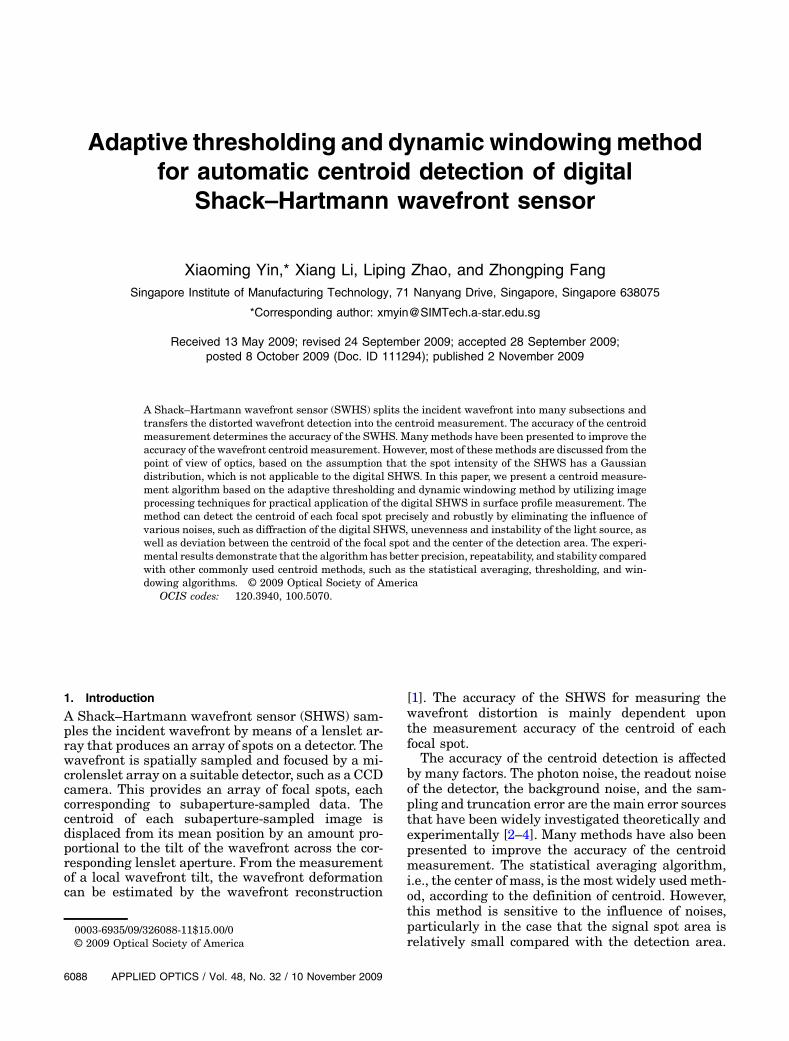
the predefined size of the detection window after thefocal spot center has been detected. Figure 3 showsthe defined focal spot subareas, detected focal spotcenters, and identified detection windows in the im-age, respectively.After that, the centroid of each focal spot is calcu-
lated using the thresholding method from the pixelswithin the detection window. But the threshold is setas the same as In, the nth high intensity value inthe focal spot subarea, which has been used as thethreshold for focal spot detection in Subsection 2.C.It is a threshold adaptive to the intensity distributionof each focal spot subarea. The calculation equationsare as follows:
xc ¼P
Ui¼1
PVj¼1ðIði; jÞ − InÞHði; jÞ · xijP
Ui¼1
PVj¼1ðIði; jÞ − InÞHði; jÞ ; ð1Þ
yc ¼P
Ui¼1
PVj¼1ðIði; jÞ − InÞHði; jÞ · yijP
Ui¼1
PVj¼1ðIði; jÞ − InÞHði; jÞ : ð2Þ
Hði; jÞ is a Heaviside function defined as
Hði; jÞ ¼�1; Iði; jÞ ≥ In
0; Iði; jÞ < In; ð3Þ
where xc and yc are the centroid position of the cer-tain focal spot, Iði; jÞ is the intensity value of the ði; jÞpixel, and In is the nth high intensity value in thisfocal spot subarea. xij and yij are the coordinates ofthe ði; jÞ pixel in the whole spot image. U and Vare the numbers of the pixels along the X and Y di-rections in the detection window.Figure 4(a) shows the centroids of focal spots de-
tected from the image shown in Fig. 2, and Fig. 4(b)shows the enlarged picture of one centroid. It can beobserved that the detected position of the centroid isquite close to the correct position in the image.
Our method actually aligns the center of the detec-tion area with the center of the focal spot by dynami-cally identifying the detection window of each focalspot based on the spot center. The method also de-tects the centorid of each focal spot using an adaptivethreshold. By aligning the center of the detectionarea with the center of the focal spot, the influenceof noise on the common averaging and windowing al-gorithms is eliminated, and the precision of the algo-rithm is improved greatly, even for a focal spotlocated far from the center of the spot subarea. Bydynamically setting the detection window and adap-tively selecting the threshold of each focal spot, theinfluences of noises such as diffraction of the digitalSHWS and instability of the light source are also re-duced, and the centroid of each focal spot can be de-tected very precisely.
Fig. 3. (Color online) Defined focal spot subareas, detected focalspot centers, and identified detection windows in the image.
Fig. 4. (Color online) (a) Detected centroids of focal spots. (b) En-larged picture of one centroid.
A software system has been developed for auto-matic centroid detection. The software can generatefocal spot subareas, detect centers of focal spots,identify detection windows, and calculate centroidsautomatically. The only parameters that need to beinput are the size of the focal spot subarea, the posi-tion of the first focal spot subarea, the intensity levelof the threshold, and the size of the detection window.The size of the focal spot subarea and the position ofthe first focal spot subarea are very easily defined inthe image, and will not affect the precision of centroiddetection. The parameters that may have significantinfluences on the precision of centroid detection arethe intensity level of the threshold and the size of thedetection window. We will study the influence ofthese two parameters in Section 3.
3. Influence of the Parameters
A. Influence of the Intensity Level of the Threshold
We change the intensity level of the threshold from 1to 40, and detect the centroid of the focal spot withevery threshold level. In this study, we fix the sizeof the detection window to 40 × 40 pixels. Figure 5shows the detected focal spots and centroids for onefocal spot shown in Fig. 2 at the threshold level ¼ 1,10, 20, 30, and 40. It can be observed from the imagethat the centroid becomes closer to the correct posi-tion with the change of the threshold level.In order to study the convergence of the algorithm
quantitatively, we calculate the absolute differencebetween the centroids detected with two adjacentthreshold levels as follows:
Δ ¼ absðCn− Cn−1Þ: ð4Þ
Here Cn is the centroid detected with thresholdlevel ¼ n, and Cn−1 is the centriod detected with thethreshold level ¼ n − 1. Figure 6 shows the adjacentdifferences of the X and Y positions of the centroidwith the change of threshold level for one spot shownin Fig. 2. It can be seen that the differences of the XandY positions both converge to 0 after the thresholdlevel is set to larger than 25.
B. Influence of the Size of the Detection Window
We change the size of the detection window from 1 to40, and detect the centroid of the focal spot in thedetection window, respectively. In this study, we fixthe threshold level to 30 as well. Figure 7 showsthe detection windows and the detected centroidsfor one spot shown in Fig. 2 at the detection windowsize ¼ 1, 10, 20, 30, and 40.
Similar to the study of the threshold level, we cal-culate the absolute difference between the centroidsdetected in two detection windows with adjacentwindow sizes as follows:
Δ ¼ absðCu− Cu−1Þ: ð5Þ
Here Cu is the centroid detected with the win-dow size ¼ u × u pixels, and Cu−1 is the centroid de-tected with the window size ¼ ðu − 1Þ × ðu − 1Þ pixels.Figure 8 shows the adjacent differences of the X andY positions of the centroid with the change of the de-tection window size for one spot shown in Fig. 2. Itcan be seen that the differences of the X and Y posi-tions converge to 0 after the window size is set tobigger than 10.
Based on the above studies, it can be con-cluded that the selections of the intensity level of
Fig. 5. (Color online) Influence of the intensity level of the threshold on the precision of centroid detection.
the threshold and the size of the detection windowhave significant influence on the precision of centroiddetection. However, the proposed centroid algorithmis certainly convergent for these two parameters. Thealgorithm can detect the centroid precisely and ro-bustly as long as these two parameters are set tosome reasonable values that are big enough to coverthe whole focal spot.
4. Experiment Results
A. Stability Experiment
We compare our centroid detection algorithm, whichis referred to as the autocentroid algorithm, withsome other commonly used algorithms, such as thestatistical averaging, thresholding, and windowing
algorithms. The parameters used in the autocentroidalgorithm are set as follows:
• the size of the focal spot subarea, 95 × 95 pixels;• the position of the first focal spot area,
(0, 0) pixel;• the intensity level of the threshold, 30; and• the size of the detection window: 40 × 40 pixels.
The same focal spot subarea generated by theautocentroid algorithm is set as the detection areaof the averaging and thresholding algorithms. Thedetection area of the windowing algorithm is definedto have the same size as the detection window usedin the autocentroid algorithm, and is centered atthe brightest pixel of each focal spot subarea. The
Fig. 6. (Color online) Differences between the centroids detected with adjacent threshold levels.
Fig. 7. (Color online) Influence of the size of the detection window on the precision of centroid detection.
threshold used in the thresholding algorithm is set to0:3Imax; here Imax is the brightest intensity value inthe focal spot subarea.The centroid detection result of the autocentroid
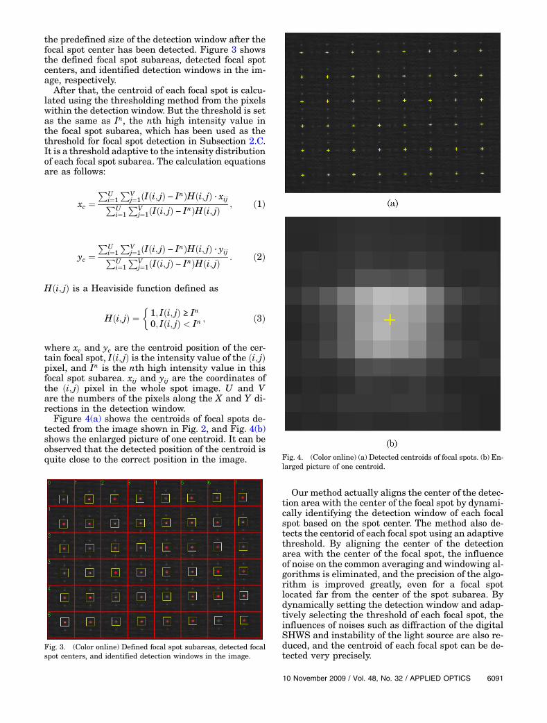
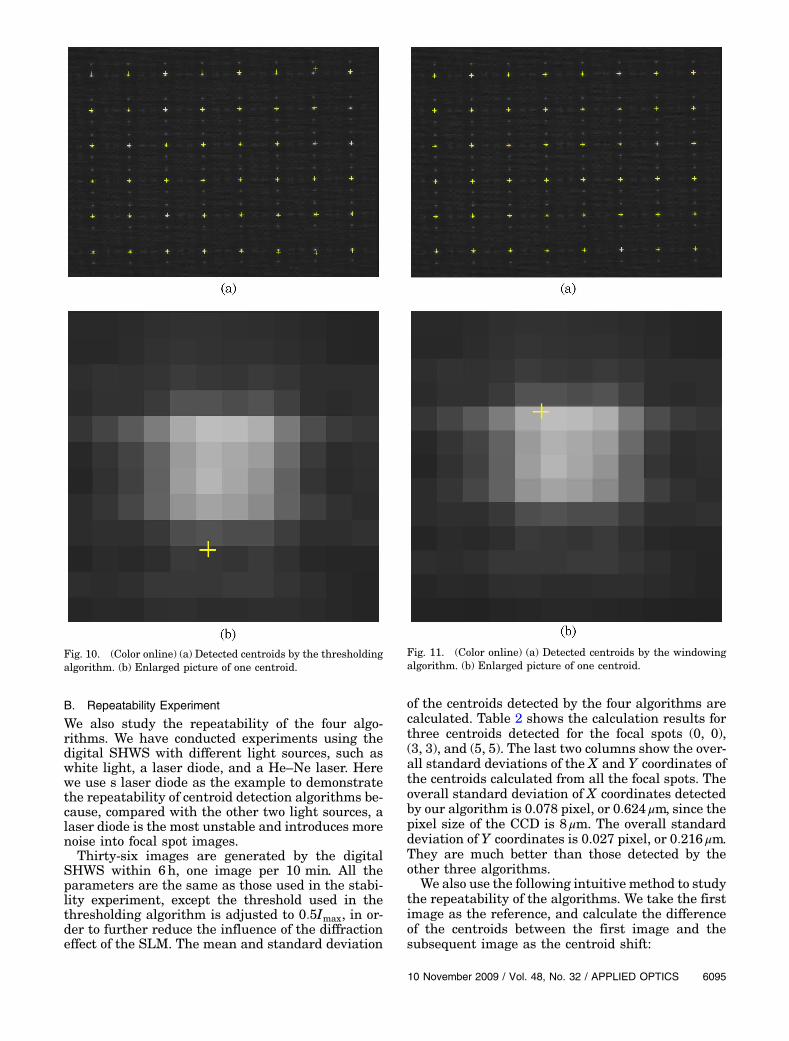
algorithm is shown in Fig. 4. Figure 9(a) shows thedetected centroids by the averaging algorithm fromthe same image shown in Fig. 2. Figure 9(b) showsthe enlarged picture of one centroid for the same fo-cal spot as shown in Fig. 4(b). Figure 10 shows thedetected centroids by the thresholding algorithm,and Fig. 11 shows the detected centroids by the win-dowing algorithm. It can be seen that some centroidsdetected by the averaging algorithm are quite farfrom the correct positions in the image because thecentroids of these spots are not at the centers of theirdetection areas. The detection precision is improvedby using the thresholding algorithm. But there arestill some centroids not locating at the correct posi-tions due to the influence of the diffraction effect ofthe digital SHWS. The centroids detected by the win-dowing algorithm are quite close to the correct posi-tions because the centers of their detection windowsare set to the brightest pixels, which are located onthe focal spots. But the precision of the windowingalgorithm is still worse than the proposed autocen-troid algorithm.At the above measurement, the position of the first
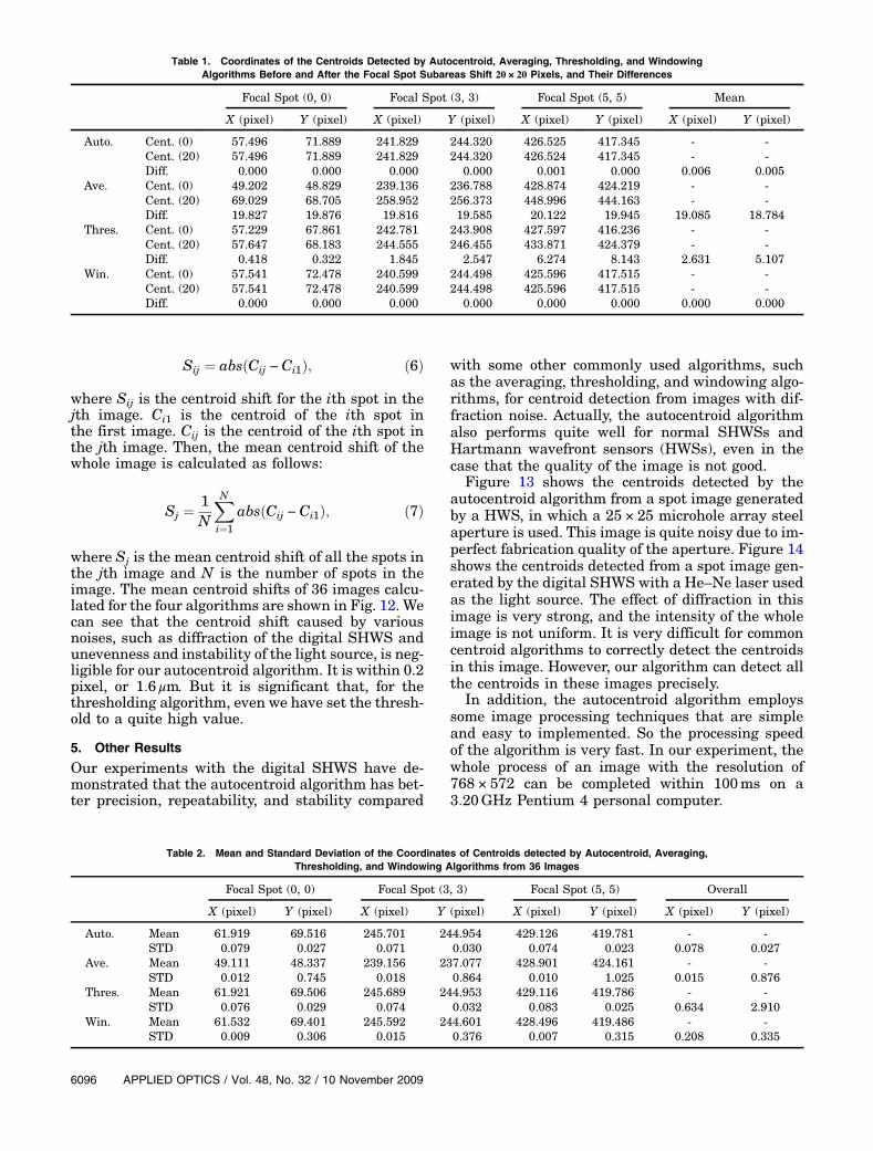
focal spot subarea is set as the default position (0, 0).Now, we reset the position of the first focal subarea to(20, 20), so that all the focal spot subareas shift20 × 20 pixels. Then we detect the centroids usingthe four algorithms again. Table 1 shows the quan-titative results of centroid detection by these four al-gorithms before and after shift. The X and Ycoordinates of the three centroids detected for thespots (0, 0), (3, 3), and (5, 5) before and after shift, aswell as their differences, are shown in Table 1. Theindex of the focal spot is shown at the upper-left cor-ners of the first row and column spot subareas, as inFig. 3. The last two columns of Table 1 show themean differences of all the centroids in the image.There is no difference between centroids detectedby the windowing algorithm before and after shift,because the brightest pixels in focal spot subareasstay the same, so that the detection areas of the cen-troids also stay the same before and after shift. We
can know from the experiments that our algorithmhas better precision and stability compared withother centroid detection algorithms.
Fig. 8. (Color online) Differences between the centroids detected in detection windows with adjacent window sizes.
Fig. 9. (Color online) (a) Detected centroids by the averaging al-gorithm. (b) Enlarged picture of one centroid.
We also study the repeatability of the four algo-rithms. We have conducted experiments using thedigital SHWS with different light sources, such aswhite light, a laser diode, and a He–Ne laser. Herewe use s laser diode as the example to demonstratethe repeatability of centroid detection algorithms be-cause, compared with the other two light sources, alaser diode is the most unstable and introduces morenoise into focal spot images.Thirty-six images are generated by the digital
SHWS within 6h, one image per 10 min. All theparameters are the same as those used in the stabi-lity experiment, except the threshold used in thethresholding algorithm is adjusted to 0:5Imax, in or-der to further reduce the influence of the diffractioneffect of the SLM. The mean and standard deviation
of the centroids detected by the four algorithms arecalculated. Table 2 shows the calculation results forthree centroids detected for the focal spots (0, 0),(3, 3), and (5, 5). The last two columns show the over-all standard deviations of the X and Y coordinates ofthe centroids calculated from all the focal spots. Theoverall standard deviation of X coordinates detectedby our algorithm is 0.078 pixel, or 0:624 μm, since thepixel size of the CCD is 8 μm. The overall standarddeviation of Y coordinates is 0.027 pixel, or 0:216 μm.They are much better than those detected by theother three algorithms.
We also use the following intuitive method to studythe repeatability of the algorithms. We take the firstimage as the reference, and calculate the differenceof the centroids between the first image and thesubsequent image as the centroid shift:
Fig. 10. (Color online) (a) Detected centroids by the thresholdingalgorithm. (b) Enlarged picture of one centroid.
Fig. 11. (Color online) (a) Detected centroids by the windowingalgorithm. (b) Enlarged picture of one centroid.
where Sij is the centroid shift for the ith spot in thejth image. Ci1 is the centroid of the ith spot inthe first image. Cij is the centroid of the ith spot inthe jth image. Then, the mean centroid shift of thewhole image is calculated as follows:
Sj ¼1N
XNi¼1
absðCij − Ci1Þ; ð7Þ
where Sj is the mean centroid shift of all the spots inthe jth image and N is the number of spots in theimage. The mean centroid shifts of 36 images calcu-lated for the four algorithms are shown in Fig. 12. Wecan see that the centroid shift caused by variousnoises, such as diffraction of the digital SHWS andunevenness and instability of the light source, is neg-ligible for our autocentroid algorithm. It is within 0.2pixel, or 1:6 μm. But it is significant that, for thethresholding algorithm, even we have set the thresh-old to a quite high value.
5. Other Results
Our experiments with the digital SHWS have de-monstrated that the autocentroid algorithm has bet-ter precision, repeatability, and stability compared
with some other commonly used algorithms, suchas the averaging, thresholding, and windowing algo-rithms, for centroid detection from images with dif-fraction noise. Actually, the autocentroid algorithmalso performs quite well for normal SHWSs andHartmann wavefront sensors (HWSs), even in thecase that the quality of the image is not good.
Figure 13 shows the centroids detected by theautocentroid algorithm from a spot image generatedby a HWS, in which a 25 × 25 microhole array steelaperture is used. This image is quite noisy due to im-perfect fabrication quality of the aperture. Figure 14shows the centroids detected from a spot image gen-erated by the digital SHWS with a He–Ne laser usedas the light source. The effect of diffraction in thisimage is very strong, and the intensity of the wholeimage is not uniform. It is very difficult for commoncentroid algorithms to correctly detect the centroidsin this image. However, our algorithm can detect allthe centroids in these images precisely.
In addition, the autocentroid algorithm employssome image processing techniques that are simpleand easy to implemented. So the processing speedof the algorithm is very fast. In our experiment, thewhole process of an image with the resolution of768 × 572 can be completed within 100ms on a3:20GHz Pentium 4 personal computer.
Table 1. Coordinates of the Centroids Detected by Autocentroid, Averaging, Thresholding, and WindowingAlgorithms Before and After the Focal Spot Subareas Shift 20 × 20 Pixels, and Their Differences
Table 2. Mean and Standard Deviation of the Coordinates of Centroids detected by Autocentroid, Averaging,Thresholding, and Windowing Algorithms from 36 Images
A SHWS splits the incident wavefront into manysubsections and transfers the distorted wavefront de-tection into the centroid measurement. The accuracyof the centroid measurement determines the accu-racy of the SHWS. Several methods have been pre-sented to improve the accuracy of the wavefrontcentroidmeasurement. However, most of thesemeth-ods are discussed from the point of view of optics, andare based on the assumption that the spot intensityof the SHWS has a Gaussian distribution, which isnot applicable to the digital SHWS. In this paper,we have presented a new centroid measurementalgorithm based on the adaptive thresholding anddynamic windowing method by utilizing image pro-cessing techniques. The algorithm can detect the cen-troid of the focal spot precisely and robustly byeliminating the influence of various noises, such asdiffraction of the digital SHWS, unevenness and in-stability of the light source, and deviation betweenthe centroid of the focal spot and the center of thedetection area.
In our method, we determine the subarea of eachfocal spot on the image directly without the need toknow the physical properties of the lenslet array.Then we detect the focal spot and calculate the centerof the focal spot using image processing techniques.After that, we dynamically identify the detectionwindow of each focal spot based on the focal spot cen-ter, and measure the centroid of each focal spot usinga threshold adaptive to the intensity distribution ofthat spot subarea.
A software system has been developed for auto-matic implementation of the algorithm. We have stu-died the influence of the input parameters on theprecision of centroid detection, and concluded thatthe selection of the parameters would not affectthe precision of centroid detection as long as theseparameters are set to some reasonable values thatare big enough to cover the whole focal spot.
Fig. 12. (Color online) Centroid shifts between the first imageand subsequent images.
Fig. 13. (Color online) Detected centroids by the autocentroid al-gorithm from a spot image generated by a Hartmann wavefrontsensor.
Fig. 14. (Color online) Detected centroids by the autocentroidalgorithm from a spot image generated by the digital Shack–Hartmann wavefront sensor with strong diffraction noise.
We also conducted stability and repeatability ex-periments using real wavefront images, and com-pared the performance of our algorithm with someother commonly used algorithms, such as the statis-tical averaging, thresholding, and windowing algo-rithms. The experimental results demonstrate thatthe presented algorithm has better precision, repeat-ability, and stability. The algorithm also performsquite well for normal SHWSs and HWSs, even inthe case that the quality of the image is not good.
References1. T. J. Kane, B. M. Welsh, and C. S. Gardner, “Wave front detec-
tor optimization for laser guided adaptive telescope,” Proc.SPIE 1114, 160–171 (1989).
2. G. Cao and X. Yu, “Accuracy analysis of a Hartmann-Shackwavefront sensor operated with a faint object,” Opt. Eng.33, 2331–2335 (1994).
3. R. Irwan and R. G. Lane, “Analysis of optimal centroid estima-tion applied to Shack–Hartmann sensing,” Appl. Opt. 38,6737–6743 (1999).
4. A. Zhang, C. Rao, Y. Zhang, and W. Jiang, “Sampling erroranalysis of Shack–Hartmann wavefront sensor with variablesubaperture pixels,” J. Mod. Opt. 51, 2267–2278 (2004).
5. S. K. Park and S. H. Baik, “A study on a fast measuring tech-nique of wavefront using a Shack–Hartmann sensor,” Opt.Laser Technol. 34, 687–684 (2002).
6. J. F. Ren, C. H. Rao, and Q. M. Li, “An adaptive thresholdselection method for Hartmann-Shack wavefront sensor,”Opto-electron. Eng. 29, 1–5 (2002).
7. S. H. Baik, S. K. Park, C. J. Kim, and B. Cha, “A center detec-tion algorithm for Shack–Hartmann sensor,” Opt. Laser Tech-nol. 39, 262–267 (2007).
8. P. Arulmozhivarman, L. P. Kumar, and A. R. Ganesan,“Measurement of moments for centroid estimation inShack-Hartmann wavefront sensor—a wavelet-based ap-proach and comparison with other methods,” Optik (Jena)117, 82–87 (2006).
9. S. A. Sallberg, B. M.Welsh, andM. C. Roggemann, “Maximuma posteriori estimation of wave-front slopes using aShack–Hartmann wave-front sensor,” J. Opt. Soc. Am. A 14,1347–1354 (1997).
10. M. A. van Dam and R. G. Lane, “Wave-front slope estimation,”J. Opt. Soc. Am. A 17, 1319–1324 (2000).
11. J. Ares and J. Arines, “Influence of thresholding on centroidstatistics: full analytical description,” Appl. Opt. 43,5796–5805 (2004).
12. Z. L. Jiang, S. S. Gong, and Y. Dai, “Numerical study ofcentroid detection accuracy for Shack–Hartmann wave-front sensor,” Opt. Laser Technol. 38, 614–619 (2006).
13. L. P. Zhao, N. Bai, X. Li, L. S. Ong, Z. P. Fang, and A. K. Asundi,“Efficient implementation of SLM as diffractive optical micro-lens array in digital Shack Hartman wavefront sensor,” Appl.Opt. 45, 90–94 (2006).