Adaptive Vectored Thrust Deorbiting of Space Debris
Ashish Tewari∗
Indian Institute of Technology, Kanpur 208016, India
DOI: 10.2514/1.A32421
A novel but simple deorbiting control system is proposed for cleaning up space debris in a low Earth orbit. The
method consists of employing a low-thrust spacecraft tug with a continuously varying thrust direction for collecting
and decelerating debris items at a given orbital radius. A time-linear thrust-direction profile is the outcome of the
nominal, two-point boundary-value problem for deceleration by a given velocity magnitude. Three simple model
reference adaptive control strategies are proposed for driving the velocity error from nominal to zero in the presence
of uncertain debrismass and rocket thrust variation.Although linear time-varying controlwith velocity feedbackand
a dead-zone is sufficient to minimize tracking error in most cases, it is improved significantly by a Lyapunov-based
controller that guarantees asymptotic stability in the presence of a random but bounded acceleration disturbance. A
nonlinear feedback adaptation law based upon the MIT rule achieves the fastest error decay rate error of the three
techniques and is seen to have a logarithmic relationship between the steady-state value of controller parameter and
adaptation gain.
Nomenclature
a = thrust acceleration, km∕s2c = controller constante = velocity error, km∕sh = orbital angular momentum, km2∕sir = unit vector in the radial directioniθ = unit vector in the tangential directionJ�·� = loss functionk = controller gainm = total instantaneous mass, kgr = position vectorr = instantaneous orbital radius jrj, kmT = thrust, Nt = time, sV�·� = Lyapunov functionα = thrust-direction angle measured from iθβ = thrust deflection angle (supplementary of α)γ = adaptation gainΔ = errorδ = thrust correction angle (control input)ε = controller deadbandθ = adaptive controller parameter�θ = boundary value for θρ = time-varying linear feedback parameter
Subscripts
0 = initial quantityf = final quantityn = pertaining to nominal trajectory
Superscript
· = time derivative
I. Introduction
S PACE debris has become amajor obstacle tomodern space flightmissions whose planning and execution includes avoidance of
large debris items, mostly in low Earth orbits (LEOs). The LEO
debris density is increasing with every launch, and unless urgentmeasures are adopted for the removal of space debris, future spacemissions will be in jeopardy. Furthermore, unplanned entry oruncontrolled deorbiting of large debris items poses a great hazard tolife and property on the ground [1,2]. Therefore, it is imperative tohave a controlled deorbiting procedure for a planned impact in aselected, unpopulated area.Any proposedmethod of debris removal must not only be accurate
insofar as desired en route trajectory and final impact location areconcerned but must also be efficient with regard to total mission cost.The requirements of accuracy and efficiency are usually conflictingin nature, thereby requiring a compromise. To deorbit space debris ina controlled manner, it is imperative to 1) rendezvous with and safelycatch each debris item, 2) have amethod of reducing the orbital speedto send the debris into a reentry trajectory, and 3) control the finalorbital speed for the desired reentry trajectory until the targetedimpact site. Both steps 1 and 2 require that the rendezvous, stationkeeping, and deorbiting maneuvers should be carried out at nearly aconstant radius while precisely controlling the speed, such that thedesired reentry conditions (inertial speed, flight path angle, velocityazimuth, latitude, longitude) are achieved at the end of the controlinterval. Maintaining a constant radius is also necessary whenmultiple items (debris field) spread at a given orbital radius are to becollected and deorbited sequentially. Clearing a debris field spreadat a given orbital radius would require repeated rendezvous withmultiple debris items. If orbital radius is changed during sucha maneuver, additional propellant would be spent to bring thespacecraft back to the original orbit for catching the next debris item.There must be an adaptive control system in place for step 3 to be
carried out for an uncertain debris mass. Several practical ways ofimplementing step 2 have been proposed in the literature, such as theuse of mechanical tethers [3], electrodynamic tethers [4], ablation bylasers [5], and propulsion by noncontact ion beams [6]. These passivetechniques can only guarantee the removal of a debris item fromthe original orbit, without having much control on either the reentrytrajectory or the latitude and longitude of ground impact [7].Furthermore, because most of the large debris items are cataloguedat nearly circular, highly inclined orbits, even a small error in theposition and velocity at the deorbit point can lead not only to a largeuncertainty in the ground track but also a risk of collision with otherdebris objects at lower radii, thereby resulting in a debris cloud.Therefore, an uncontrolled (or partially controlled) deorbiting canincrease (rather than decrease) the hazards of space debris.General spacecraft orbital maneuvers involve orbital shape, size,
and plane control for relative motion in orbit. Typically, an orbitalmaneuver consists of an impulsive rocket thrust applied in a constantdirection relative to the flight path, both at the beginning and theend of a fixed control interval, thereby resulting in a two-point
boundary-value problem (2PBVP) with practical solutions such asHohmann transfer [8], Lambert transfer [9], andClohessey–Wiltshireapproximation [10] for relative orbital motion. However, the tradi-tional bang–coast–bang, elliptical trajectories would be inapplicablein a space debris cleanup mission where capturing and deorbitingmultiple debris items at a nearly constant orbital radius is involved.Although a Hohmann maneuver would require an infinite time for aconstant radius transfer, neither the Lambert nor the Clohessey–Wiltshire problem has a solution in such a case. One could possiblyenvisage a multi-impulse maneuver where a spacecraft approachesthe targeted debris item from a higher (or lower) initial orbit in anelliptical transfer orbit and catches the debris item (or interacts with itin some manner) at the perigee (or apogee) while simultaneouslyapplying a deorbit impulse of just the right amount to send it into aplanned impact zone. However, it is quite difficult to design anautonomous guidance and control system for such a mission. Asimpler maneuver would consist of approaching the debris, linkingup with it, and decelerating it, all at a nearly constant radius. Avariable-speed, constant-radius maneuver can be produced by avariable thrust magnitude, a variable thrust direction, or both.However, it is more practical to control the thrust direction rather thanthe thrust magnitude of a rocket engine.This paper presents a nonlinear orbital control strategywith the use
of a space tug that can apply a constant acceleration in a directionvarying linearly with time to maintain a constant radius while linkingup with and decelerating the debris object by a desired velocitymagnitude. The advantage of this method is that both the positionand velocity of atmospheric entry (thus the resulting trajectory untilimpact) can be precisely controlled. The method is especially usefulwhen a single spacecraft is employed for sweeping and collectingmultiple debris items spread out at a nearly constant orbital radius.Such a spacecraft is envisaged to be either a small, unmanned, single-stage-to-orbit vehicle or a modified reattachable module of theInternational Space Station, which will not produce any space debrisof its own. Other situations where the constant-radius maneuver canbe applied are pulling out dead satellites from geosynchronous Earthorbit and rendezvous missions where flyby of another spacecraft atnearly the same altitude is involved.Because the proposed space deorbiting mission must be fully
autonomous, it is important to consider robustness and adaptationof the control system to parametric variations in the plant. Suchvariations will naturally arise due to lack of precise knowledge ofdebris mass. Furthermore, random variations in the rocket thrust arealways present, which makes the applied acceleration an uncertain(but bounded) parameter. Our attempt in this paper is to devisefeedback-control strategies that can adapt to the plant parametricvariations and yet produce asymptotic stability. For this purpose,three different closed-loop designs are presented for driving anyvelocity error from the nominal to zero. These include a Lyapunov-based technique [11] as well as that based upon the MIT rule [12] forminimizing the velocity error by a nonlinear adaptation mechanism.
II. Nominal Trajectory Model
To derive the nominal trajectory for the deorbital maneuver,consider an appropriate plant model and its solution to the boundaryconditions prescribed at either end of the control interval, t ∈ �0; tf �.At t � 0, the spacecraft is assumed to be in contact with and travelingat the same speed as the debris item, while at t � tf, the deorbitmaneuver is ended and the debris item is released and beginstraveling in an elliptical orbit for reentry. The subscripts 0 and findicate quantities at the beginning and the end of the maneuver,respectively.
A. Orbital Plant
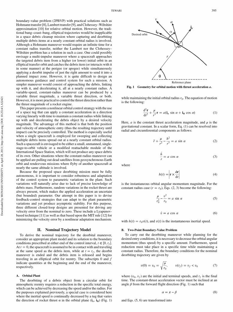
The deorbiting of a debris object from a circular orbit foratmospheric reentry requires a reduction in the specific total energy,which can be achieved by decreasing the speed and/or the radius. Forthe purposes explained previously, a special case is considered herewhere the inertial speed is continually decreased by a tug that variesthe direction of rocket thrust α in the orbital plane (ir, iθ) (Fig. 1)
whilemaintaining the initial orbital radius r0. The equation ofmotionis the following:
d2r
dt2� μ
r3r � a�ir sin α� iθ cos α� (1)
Here, a is the constant thrust acceleration magnitude, and μ is thegravitational constant. In a scalar form, Eq. (1) can be resolved intoradial and circumferential components as follows:
�r� μ
r2−h2
r3� a sin α (2)
_h
r� a cos α (3)
where
h�t� �����r × dr
dt
���� (4)
is the instantaneous orbital angular momentum magnitude. For theconstant radius case (r � r0), Eqs. (2, 3) become the following:
μ
r20−v2
r0� a sin α (5)
_v � a cos α (6)
with h�t� � r0v�t�, and v�t� is the instantaneous inertial speed.
B. Two-Point Boundary-Value Problem
To carry out the deorbiting maneuver while planning for thedesired entry conditions, it is necessary to decrease the orbital angularmomentum (thus speed) by a specific amount. Furthermore, speedreduction must take place in a specific time while maintaining aconstant radius. Therefore, the boundary conditions for the nominaldeorbiting trajectory are given by
v�0� � v0 ������μ
r0
r; v�tf� � vf < v0 (7)
where (v0, vf) are the initial and terminal speeds, and tf is the finaltime. The constant-thrust acceleration vector must be inclined at anangle β from the forward flight direction (Fig. 1) such that
α � π − β (8)
and Eqs. (5, 6) are transformed into
ir i
v a
r
θ
Desired orbit
Reference plane
Fig. 1 Geometry for orbital motion with thrust acceleration a.
TEWARI 395
Dow
nloa
ded
by M
ON
ASH
UN
IVE
RSI
TY
on
Apr
il 28
, 201
3 | h
ttp://
arc.
aiaa
.org
| D
OI:
10.
2514
/1.A
3242
1
v20 − v2
r0� a sin β (9)
_v � −a cos β (10)
Differentiation of Eq. (9) with time and substitution of Eq. (10) yieldsthe following relationship between the instantaneous speed and thrustdirection:
_β � 2v
r0(11)
Repeating the process of differentiation and substitution of Eq. (10)results in the following nonlinear, ordinary differential equation forthrust direction β�t�:
�β� 2a
r0cos β � 0 (12)
which must be solved subject to the boundary conditions [Eq. (7)],which by Eq. (11) become
_β�0� � 2v0r0; _β�tf� �
2vfr0
(13)
Equations (14) and (15) constitute a 2PBVP for the thrust-directioninput profile β�t� that can be solved using either a shooting or acollocation technique [9]. A sample solution for Earth withr0 � 6900 km, vf � 0.99v0, a � 1 m∕s2 and for various values oftf ranging 60–240 s is plotted in Fig. 2. The approximately time-linear thrust-direction profile with a nearly constant slope is evidentin all cases for which the maximum deflection is limited toβ�t� < 90 deg. This is an important result that indicates that thecontroller implementation is possible by a simple timing (orclockwork) mechanism (as opposed to online 2PBVP computation).In addition to the thrust direction, the velocity profile is also time-linear up to tf � 120 s but becomes nonlinear for longer controlintervals. Clearly, themost efficient maneuver among these is the onewith the shortest control interval (tf � 60 s), resulting in not only thesmallest propellant expenditure for the given 1% speed reduction butalso the smallest thrust deflection angle β�t�.
C. Time-Linear Solutions
It is clear fromFig. 2 that the solution to the 2PBVPassociatedwitha constant-radius deceleration produces nearly time-linear profilesfor a reasonably small deceleration magnitude. To further investigatethis fact, observe that the boundary conditions given by Eq. (13) forrepresentative numerical values of r0, v0, and vf corresponding to an
Earth orbit translate into nearly the same slope of the thrust-directionangle at both the ends of the control interval. Furthermore, themultiplier of cos β in Eq. (12) is quite small for a realistic thrustacceleration a,
2a
r0≃ 0 (14)
thereby implying that a time-linear (ramp) approximation for thethrust angle,
β�t� ≃ 2v0r0t� β�0� (15)
would reasonably satisfy both the differential equation and theboundary conditions for any value of the initial angle β�0�. Theaccuracy of the approximation, of course, depends upon the selectedvalue of β�0�. A practical method of determining the correct initialthrust angle as a function of the final time tf is an interpolation of the2PBVP solution of Fig. 2, such as that by the following polynomial:
β�0� �XNk�0
cktkf (16)
A comparison of the least-squares curve fit of Eq. (16) with N � 3and the 2PBVP data is shown in Fig. 3. A thrust-direction programgiven by such a polynomial interpolation can be easily implementedin the flight-control hardware. An alternativemethod of obtaining theapproximate initial thrust direction is by substituting Eq. (15) intoEq. (10) and integrating in time, which yields the followingtranscendental equation for β�0�:
sin
�2v0r0tf � β�0�
�− sin β�0� �
2v0�v0 − vf�ar0
(17)
Equation (17) is no more complex than Kepler’s equation [8] andcan be solved for β�0� by an appropriate iterative technique such asNewton’s method, with the usual drawback of sensitivity to initialguess that may make it cumbersome for real-time computation. Ofcourse, it is possible to replace the actual 2PBVP solution by theapproximate solution to Eq. (17) and then employ the least-squarescurve fit of Eq. (16) for a practical implementation. A flowchart forthe nominal deorbiting procedure is shown in Fig. 4.
III. Model Reference Adaptation
If there were no errors in applying the desired thrust input and thedebris mass were precisely known, the nominal time-linear profile of
100
0 50 150100 200 250-50
0
50
Time (s)
β (d
eg)
tf=60 s
tf=120 s
tf=180 s
tf=240 s
8
150
7.5
7
6.50 50 100
Time (s)
v (k
m/s
)
200 250
Fig. 2 Numerical solution of the two-point boundary-value problem
associated with a vectored thrust deceleration in Earth orbit while
maintaining constant radius of 6900 km.
Fig. 3 Least-squares polynomial fit of the 2PBVP numerical solution
shown in Fig. 2.
396 TEWARI
Dow
nloa
ded
by M
ON
ASH
UN
IVE
RSI
TY
on
Apr
il 28
, 201
3 | h
ttp://
arc.
aiaa
.org
| D
OI:
10.
2514
/1.A
3242
1
the previous section would by itself be sufficient in controlling thedeorbit trajectory. However, the uncertainty in the mass of debris aswell as the presence of imperfections in the thrust-actuatingmechanism require a corrective control input that is applied in anadaptive, feedback loop. The design of such a control system is theobjective of the present section. Before beginning the design for anadaptive controller, certain distinctive features of the nominal orbitalplant that enable a systematic analysis are noted.Remark 1: The assumption of Eq. (14) is valid for a small but
varying thrust acceleration a. Thus, the assumption of constant a isunnecessary for obtaining a time-linear thrust-direction profile.Remark 2: When an appreciable propellant mass is consumed
during the maneuver, the thrust acceleration a cannot be taken asconstant.Remark 3: The thrust acceleration a cannot be predicted a priori
due to the uncertain debris mass. In such a case, there is a need toaccount for the total mass of spacecraft and debris as an unknownfunction of time, m�t�.With a rocket engine of a fixed nozzle geometry, a given propellant
burn rate _m, and exhaust speed ve, the thrust T is nearly a constant,which results in
T � − _mve � ma � −m _v
cos β(18)
The achieved deceleration is a function of the instantaneous totalmass, which is an uncertain parameter depending upon the size ofdebris. When an additional disturbance is present due to the off-design thrust and/or a misaligned nozzle, the final trajectory woulddepart significantly from nominal, which can still be regarded astime-linear in view of remark 1. To follow a given nominal trajectory,the thrust angle must therefore adjust according to actual thrust andmass by an appropriate closed-loop adaptation law. Three separatemodel reference techniques are proposed here based upon thenominal time-linear control profile. Let the uncertain mass as well asthe thrust, respectively, be given by the following:
m � mn �Δm (19)
T � Tn � ΔT (20)
whereTn � − _mnve is the design thrust for the given constant exhaustspeed ve, resulting in the nominal mass profile,
mn � m0 −Tnvet (21)
and Δm, ΔT are bounded random perturbations. To adapt to modeluncertainties, the corrected thrust direction is given by
β � βn � δ (22)
where βn�t� is the nominal profile given by Eq. (15), and δ�t� is asmall correction angle. By expanding cos β with Eq. (22) about thenominal profile, it is possible to write
δ sin βn � cos βn − cos β (23)
And, by substituting Eq. (18), the linear time-varying plant is givenby
_e � δ����������������a2n − _v2n
q��_vnan
�Δa (24)
where
e � v − vn (25)
is the instantaneous velocity error, and the thrust acceleration is
a � T
m� an � Δa (26)
with an�t� � Tn∕mn�t� being the nominal acceleration. Clearly, thevelocity error is governed by the random acceleration error Δa�t�,regarded as the unknown parameter with the following upper bound:
Contact debris for deorbiting into selected
impact region
Determine deorbiting point for given tf
Is sufficient propellant available
for maneuver?
Stop
Yes
No
Compute initial thrust direction, (0)β
Apply constant slope, time-linear thrust profile, (t)β , to decelerate and release
the debris item for a planned re-entry.Cycle the tug for rendezvous with new debris with ( )tβ and make contact.
Select new debris item and compute propellant mass required for rendezvous and deorbiting.
Fig. 4 Deorbiting algorithm with time-linear thrust direction for multiple debris cleanup.
TEWARI 397
Dow
nloa
ded
by M
ON
ASH
UN
IVE
RSI
TY
on
Apr
il 28
, 201
3 | h
ttp://
arc.
aiaa
.org
| D
OI:
10.
2514
/1.A
3242
1
jΔa�t�j ≤ Δa∞ (27)
Aclosed-loop adaptation law is to be derived for the control input δ�t�that can drive the speed error to zero in the presence of the uncertainparametric disturbance Δa�t�. A schematic diagram of the closed-loop system is depicted in Fig. 5.
A. Linear Feedback
A simple adaptation approach based on the following linearfeedback law is first investigated:
δ � _vn
an����������������a2n − _v2n
p ρe; � _v2n ≠ a2n� (28)
where it is assumed that velocity error e�t� is available formeasurement and ρ�t� is the controller parameter. By substitutingEq. (28) into Eq. (24), the following linear, time-varying closed-loopstate equation results for velocity error:
_e ��_vnan
��ρe� Δa� (29)
Remark 4: Because _vn�t�∕an�t� < 0 for deorbiting, a choice ofconstant parameter ρ > 0 will stabilize the system but cannot makethe error vanish in the steady state. Thus, the closed-loop system isnot asymptotically stable in the presence of randomacceleration errorΔa�t�. A practical choice for the controller parameter isρ � kΔa∞∕je�0�j, where k > 0 is a constant gain and je�0�j is thelargest possible initial speed error.Remark 5: It is possible for small thrust angles βn�t� that _vn ≃ −an;
see Eq. (10). In such a case, the control law of Eq. (28) would result inan arbitrarily large correction angle (control input) δ�t� if appliedunmodified. Because the error-state equation Eq. (24) becomes _e ≃Δa for _vn ≃ −an, irrespective of δ�t�, it is prudent to have δ � 0whenever the nominal value of thrust deflection angle βn�t� becomessmall. This is practically implemented by putting a dead zone aroundβn�t� � 0 as follows:
δ �(
_vn
an����������a2n− _v2np ρe; �βn > ε�
0; �βn ≤ ε�(30)
Remark 6: Because a precise measurement and feedback of thevelocity error is impossible, the robustness of the control strategywith respect to a small but random measurement noise must bestudied. This can be carried out via a Gaussian model.
B. Lyapunov-Based Feedback
The uniform stability of linear, time-varying feedback in thepresence of a bounded acceleration error using the Lyapunov stability
theorem [11] is next demonstrated as an alternative to the linearfeedback adaptation considered previously.Proposition 1: Let the random acceleration disturbance be
bounded by an unknown magnitude Δa∞, given by Eq. (27). Then,the control law,
δ � −e����������������
a2n − _v2np �
c� k _v2na2n
�; � _v2n ≠ a2n� (31)
where c > 0, k > 0 are controller constants, results in a global anduniform convergence of the velocity error e�t� to the followingcompact region in the limit t→ ∞:
R ��e∶ jej ≤ Δa∞
2�����kcp
�(32)
Proof: Let us select the following candidate Lyapunov function:
V�e� � 1
2e2 (33)
By substituting the control law, Eq. (31), into the linearized errorequation, Eq. (24), the following closed-loop dynamics results:
_e � −�c� k _v2n
a2n
�e�
�_vnan
�Δa � f�e; t� (34)
It is noted that, in view of Eq. (27), f�e; t� is locally Lipschitz in e andt. Furthermore, V�e� is radially unbounded and has time derivative
_V � e _e � −�c� k _v2n
a2n
�e2 �
�_vnan
�Δae
� −ce2 − k�_vnane −
Δa2k
�2
� �Δa�2
4k
or, by substituting Eq. (27),
_V ≤ −ce2 � �Δa∞�2
4k(35)
Because _V < 0 whenever
jej > Δa∞2
�����kcp (36)
the velocity error magnitude je�t�j decreases uniformly and globallyin the limit t→ ∞ by the LaSalle–Yoshizawa theorem [11].Therefore, e�t� is bounded and converges uniformly and globally tothe compact set, Eq. (32), as t→ ∞.
Fig. 5 Schematic block diagram of closed-loop deorbiting system.
398 TEWARI
Dow
nloa
ded
by M
ON
ASH
UN
IVE
RSI
TY
on
Apr
il 28
, 201
3 | h
ttp://
arc.
aiaa
.org
| D
OI:
10.
2514
/1.A
3242
1
Note that global stability is demonstrated without knowing thebound on the acceleration error, as long as sufficiently largevalues forc and k, are selected to satisfy the inequality of Eq. (36) for anarbitrarily small velocity error. However, in the presence of a nonzeroacceleration error bounded by Δa∞, the velocity error would remainnonzero.Proposition 2: Let the random acceleration disturbance be
bounded by a known magnitude Δa∞. Then, the control law,
δ � −e����������������
a2n − _v2np �
c�Δa∞_vnan
�; � _v2n ≠ a2n� (37)
where c > 0 is a controller constant, results in a global, asymptotic,and uniform convergence of the velocity error e�t� to zero in the limitas t→ ∞.Proof : Follows easily from the proof of proposition 1 by replacing�k _vn
an� by Δa∞ in Eq. (34).
Thus, by using the knowledge of the acceleration error bound,global asymptotic stability can be achieved.
C. Nonlinear Feedback by the MIT Rule
Finally, a nonlinear model reference adaptation technique, calledthe MIT rule [12], is considered, which drives the loss function,
J�θ� � 1
2e2 (38)
to zero by adjusting the controller parameter θ�t� along the directionof the negative gradient of J,
_θ � −γ∂J∂θ� −γe
∂e∂θ
(39)
Here, γ > 0 is a constant adaptation gain. The sensitivity function∂e∕∂θ can be expressed as follows:
∂e∂θ� _e
_θ(40)
which, substituted into Eq. (32), yields
_θ2 � −γe _e (41)
The feedback law of Eq. (28) is modified for the present case asfollows:
δ � _vn
an����������������a2n − _v2n
p θe; � _v2n ≠ a2n� (42)
which is now a nonlinear one due to the variation of θ�t� with thevelocity error e�t�. Finally, by substituting Eq. (42) and the errorequation [Eq. (24)] with Δa � 0 into Eq. (40), the followingnonlinear adaptation law is obtained:
_θ � �e
�����������������������−γ�_vnan
�θe
s(43)
Remark 7: In view of remark 4, note that the square root in Eq. (43)is real for θ > 0, which is also necessary for closed-loop stability.Therefore, the appropriate sign on the right-hand side of Eq. (43)should be taken to avoid a crossing of θ � 0, thereby maintainingθ > 0 at all times. A practical adaptation algorithm for this purpose isthe following:
_θ �
8>>>>><>>>>>:e
�������������������−γ�
_vnan
�θ
s; �θ > �θ�
jej�������������������−γ�
_vnan
��θ
s; �θ ≤ �θ�
(44)
Thus, we have introduced a boundary layer of thickness �θ > 0 fordriving θ�t� away from the boundary at θ � 0 when e�t� → 0. Ofcourse, the success of the scheme in the presence of randomacceleration error depends upon a suitable initial choice, θ�0�, such asthat discussed in remark 4. Furthermore, remarks 5 and 6 are stillvalid here. Hence, while the convergence of adaptation scheme isimproved in comparison with the linear adaptation law, the singu-larity at small nominal thrust angles is still present and should beavoided by taking a reasonably large terminal time in the nominalprofile. Robustness of the nonlinear closed-loop system to measure-ment noise is more problematic than the linear approach consideredpreviously.
IV. Numerical Results
Consider the tracking of a nominal profile for Earth orbit withr0 � 6900 km, a � 1:756 m∕s2, vf � 0.9v0 and tf � 600 s, forwhich the 2PBVP solution yields a nearly time-linear thrust-directionprofile with the initial and final values of β�0� � −1.447 deg andβ�tf� � 74.762 deg., respectively. Compared with an impulsive,tangential maneuver for the same speed change (760.1 m∕s), theconstant-radius burn is equivalent to a total velocity impulse of1053.6 m∕s, or about 39% larger propellant mass with the samespecific impulse. As discussed earlier, the propellant consumptioncan be reduced significantly by taking a smaller value of tf. Thenominal rocket thrust and exhaust speed are taken to beTn � 1756 Nand ve � 3500 m∕s, and the nominal initial mass ism0 � 1000 kg.The closed-loop trajectory is simulated with normally distributedrandom variation (with standard deviation 25% of mean) in thethrust acceleration a � T∕m, caused by uncertain payload massand thrust magnitude, beginning with an initial speed error ofe�0� � 0.01 km∕s, which represents an extreme case rather than theexpected value in a real maneuver, to test the adaptation laws. Thenominal velocity and thrust-direction profiles are stored, and afourth-order, fifth-stage Runge–Kutta solver is employed to integratethe closed-loop state equations.Consider first the linear feedback control law Eq. (28) with the
following controller parameter:
ρ�t� � 0.25kan�t�je�0�j
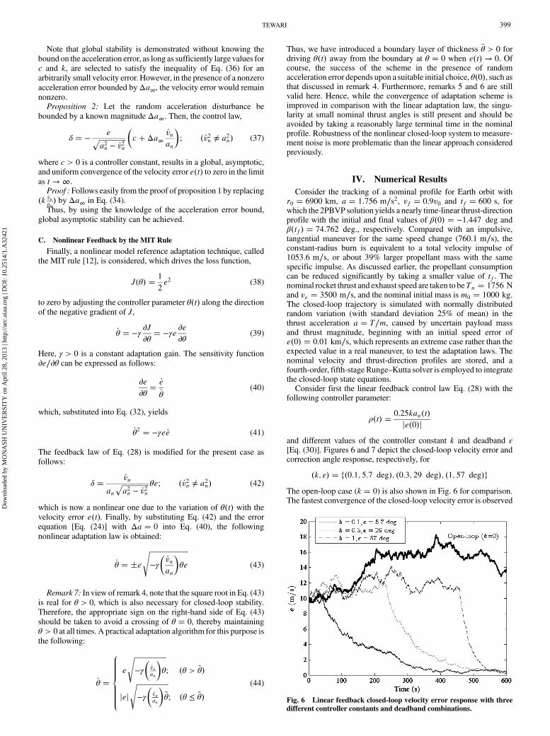
and different values of the controller constant k and deadband ε[Eq. (30)]. Figures 6 and 7 depict the closed-loop velocity error andcorrection angle response, respectively, for
The open-loop case (k � 0) is also shown in Fig. 6 for comparison.The fastest convergence of the closed-loop velocity error is observed
Fig. 6 Linear feedback closed-loop velocity error response with three
different controller constants and deadband combinations.
TEWARI 399
Dow
nloa
ded
by M
ON
ASH
UN
IVE
RSI
TY
on
Apr
il 28
, 201
3 | h
ttp://
arc.
aiaa
.org
| D
OI:
10.
2514
/1.A
3242
1
for the case of �k; ε� � �0.1; 5.7 deg� for which the control actionbegins the earliest (t � 53.5 s). However, this is also the casewith thelargest required control power. Even when the control action isdelayed as long as 450 s, there is a rapid reduction in the velocity errorwith the large random thrust acceleration perturbation. The overshootand the transient oscillations are seen to increase the longer thecontrol is delayed. This study reveals the adequacy of linear feed-back strategy for adaptive control, provided the robustness withmeasurement noise is taken into consideration.The Lyapunov-based design is simulated next using the control
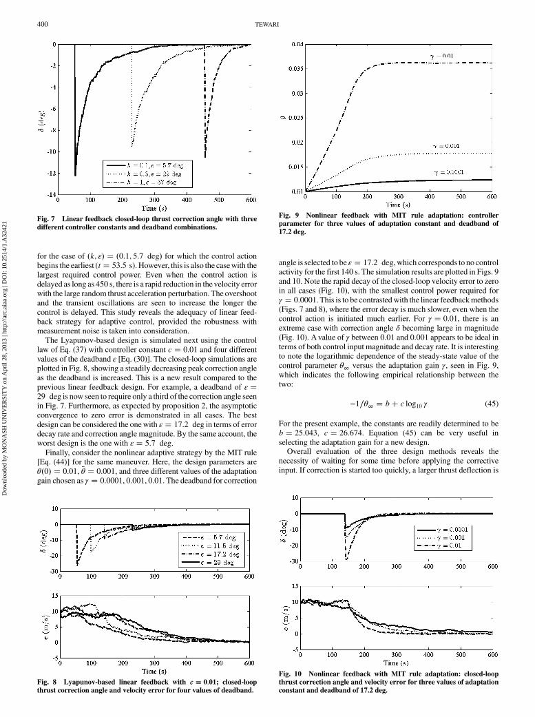
law of Eq. (37) with controller constant c � 0.01 and four differentvalues of the deadband ε [Eq. (30)]. The closed-loop simulations areplotted in Fig. 8, showing a steadily decreasing peak correction angleas the deadband is increased. This is a new result compared to theprevious linear feedback design. For example, a deadband of ε �29 deg is now seen to require only a third of the correction angle seenin Fig. 7. Furthermore, as expected by proposition 2, the asymptoticconvergence to zero error is demonstrated in all cases. The bestdesign can be considered the onewith ε � 17.2 deg in terms of errordecay rate and correction angle magnitude. By the same account, theworst design is the one with ε � 5.7 deg.Finally, consider the nonlinear adaptive strategy by the MIT rule
[Eq. (44)] for the same maneuver. Here, the design parameters areθ�0� � 0.01, �θ � 0.001, and three different values of the adaptationgain chosen as γ � 0.0001, 0.001, 0.01. The deadband for correction
angle is selected to be ε � 17.2 deg, which corresponds to no controlactivity for the first 140 s. The simulation results are plotted in Figs. 9and 10. Note the rapid decay of the closed-loop velocity error to zeroin all cases (Fig. 10), with the smallest control power required forγ � 0.0001. This is to be contrastedwith the linear feedbackmethods(Figs. 7 and 8), where the error decay is much slower, even when thecontrol action is initiated much earlier. For γ � 0.01, there is anextreme case with correction angle δ becoming large in magnitude(Fig. 10). Avalue of γ between 0.01 and 0.001 appears to be ideal interms of both control input magnitude and decay rate. It is interestingto note the logarithmic dependence of the steady-state value of thecontrol parameter θ∞ versus the adaptation gain γ, seen in Fig. 9,which indicates the following empirical relationship between thetwo:
−1∕θ∞ � b� c log10 γ (45)
For the present example, the constants are readily determined to beb � 25.043, c � 26.674. Equation (45) can be very useful inselecting the adaptation gain for a new design.Overall evaluation of the three design methods reveals the
necessity of waiting for some time before applying the correctiveinput. If correction is started too quickly, a larger thrust deflection is
Fig. 7 Linear feedback closed-loop thrust correction angle with three
different controller constants and deadband combinations.
Fig. 8 Lyapunov-based linear feedback with c � 0.01; closed-loop
thrust correction angle and velocity error for four values of deadband.
Fig. 9 Nonlinear feedback with MIT rule adaptation: controller
parameter for three values of adaptation constant and deadband of
17.2 deg.
Fig. 10 Nonlinear feedback with MIT rule adaptation: closed-loop
thrust correction angle and velocity error for three values of adaptation
constant and deadband of 17.2 deg.
400 TEWARI
Dow
nloa
ded
by M
ON
ASH
UN
IVE
RSI
TY
on
Apr
il 28
, 201
3 | h
ttp://
arc.
aiaa
.org
| D
OI:
10.
2514
/1.A
3242
1
required for the same accuracy in the steady-state. The decay rate ofvelocity error can bemaximized by suitably adjusting the adaptation/controller constants as well as the time delay before applying thecorrective input. Clearly, of the three adaptation methods consideredhere, the MIT rule achieves the fastest error decay rate and is also thesimplest to implement.
V. Conclusions
An adaptive thrust-deflection control system for maintaining nearconstant radius for station keeping with, collecting, and dece-lerating space debris smoothly in the presence of mass and thrustuncertainties is quite feasible. The required propellant consumptionis 30–40% larger than that required for an impulsive, tangential thrustmaneuver and can be decreased by suitably selecting a smaller burntime. However, the total propellant cost rather than that required by asingle debris deorbiting should be considered for a realistic estimateof the overall efficiency. It is to be reiterated here that a constant-radius burn offers a greater controllability over the final reentrycondition (hence en route trajectory and impact location) over that ofa traditional, tangential, impulsive maneuver. Perhaps an exhaustivestudy of this comparison can be conducted in a future paper applied toa real deorbitingmission. The resulting time-linear profile for varyingthrust direction requires nothing more complex than an onboardtiming (clockwork) mechanism, whereas even nonlinear feedbackadaptation schemes, such as the MIT rule, are simple to implementwith suitable choices of adaptation gains and time delays. Althougha single-stage-to-orbit space tug may be a little distant on thetechnological horizon, a suitably modified spacecraft based upon theProgress, Soyuz, or SpaceX module can be released from theInternational Space Station for capturing and deorbiting debris itemsin the manner suggested here. It is thought that the technology ispresently available for such a practical and cost-effective removalmethod, and it can be applied urgently to the increasingly alarmingproblem of space debris accumulation, rather than waiting for afuturistic concept for which much more research needs to beperformed. The concept of maneuvering a spacecraft by time-linearthrust vectoring can be extended to othermissionswhere autonomouspositioning and station keeping between two or more objects isrequired.
References
[1] Mendeck, G. F., and Kadwa, B., “Public Life Risk Assessmentof Off-Nominal Genesis Entries,” Advances in Astronautical Sciences,American Astronautical Society, San Diego, 2005, pp. 1923–1938.
[2] Patera, R. P., “Hazard Analysis for Uncontrolled Space VehicleReentry,” Journal of Spacecraft and Rockets, Vol. 45, No. 5, 2008,pp. 1031–1041.doi:10.2514/1.30173
[3] Nishida, S., Kawamoto, S., Okawa, Y., Terui, F., and Kitamura, S.,“Space Debris Removal System Using a Small Satellite,” Acta
Astronautica, Vol. 65, Nos. 1–2, 2009, pp. 95–102.doi:10.1016/j.actaastro.2009.01.041
[4] Takeichi, N., “Practical Operation Strategy for Deorbit of anElectrodynamic Tethered System,” Journal of Spacecraft and Rockets,Vol. 43, No. 6, 2006, pp. 1283–1288.doi:10.2514/1.19635
[5] Phipps, C. R., and Reilly, J. P., “ORION: Clearing Near-Earth SpaceDebris in Two Years Using a 30-kW Repetitively-Pulsed Laser,”Proceedings of XI International Symposium onGas Flow andChemical
Lasers and High-Power Laser Conference, Vol. 3092, InternationalSociety for Optical Engineering (SPIE), San Diego, CA, 1997,pp. 728–731.
[6] Bombardelli, C., and Pellaez, J., “Ion Beam Shepherd for ContactlessSpace Debris Removal,” Journal of Guidance, Control, and Dynamics,Vol. 34, No. 3, 2011, pp. 916–920.doi:10.2514/1.51832
[7] Tewari,A., “EntryTrajectoryModelwith ThermomechanicalBreakup,”Journal of Spacecraft and Rockets, Vol. 46, No. 2, 2009, pp. 299–306.doi:10.2514/1.39651
[8] Battin, R. H., An Introduction to the Mathematics and Methods of
[9] Tewari, A., Advanced Control of Aircraft, Spacecraft and Rockets,Wiley, Chichester, England, U.K., 2011, pp. 297–355, Chap. 6.
[10] Clohessey,W. H., andWiltshire, R. S., “Terminal Guidance Systems forSatellite Rendezvous,” Journal of the Aerospace Sciences, Vol. 27,Sept. 1960, pp. 653–658.
[11] Krstic, M., Kanellakopoulos, I., and Kokotovic, P., Nonlinear and
Adaptive Control Design, Wiley-Interscience, New York, 1995,Chap. 2.
[12] Astrom, K. J., andWittenmark, B., Adaptive Control, Addison-Wesley,Reading, MA, 1995, pp. 185–260, Chap. 5.