Additional Experiments for

Communication

System Design

Using DSP

Algorithms

with Laboratory Experiments

for the TMS320C6713 DSK

Steven A. Tretter

Steven A. TretterDepartment of Electrical and Computer EngineeringUniversity of MarylandCollege Park, MD 20742tretter@umd.edu

c© 2010 Steven A. Tretter

Contents

19 Continuous-Phase Frequency Shift Keying (FSK) 119.1 Definition of the FSK Signal . . . . . . . . . . . . . . . . . . . . . . . . . . . 119.2 Power Spectral Density for an FSK Signal . . . . . . . . . . . . . . . . . . . 319.3 FSK Demodulation . . . . . . . . . . . . . . . . . . . . . . . . . . . . . . . . 6

19.3.1 An Exact Frequency Discriminator . . . . . . . . . . . . . . . . . . . 719.3.1.1 Symbol Clock Acquisition and Tracking . . . . . . . . . . . 9

19.3.2 A Simple Approximate Frequency Discriminator . . . . . . . . . . . . 1019.3.3 The Phase-Locked Loop . . . . . . . . . . . . . . . . . . . . . . . . . 1019.3.4 Optimum Noncoherent Detection by Tone Filters . . . . . . . . . . . 12

19.3.4.1 Discrete-Time Implementation . . . . . . . . . . . . . . . . 1419.3.4.2 Recursive Implementation of the Tone Filters . . . . . . . . 1519.3.4.3 Simplified Demodulator for Binary FSK . . . . . . . . . . . 1619.3.4.4 Generating a Symbol Clock Timing Signal . . . . . . . . . . 17

19.4 Symbol Error Probabilities for FSK Receivers . . . . . . . . . . . . . . . . . 2419.4.1 Orthogonal Signal Sets . . . . . . . . . . . . . . . . . . . . . . . . . . 24

19.5 Experiments for Continuous-Phase FSK . . . . . . . . . . . . . . . . . . . . 2519.5.1 Theoretical FSK Spectra . . . . . . . . . . . . . . . . . . . . . . . . . 2519.5.2 Making FSK Transmitters . . . . . . . . . . . . . . . . . . . . . . . . 26

19.5.2.1 Initial Handshaking Sequence . . . . . . . . . . . . . . . . . 2619.5.2.2 Simulating Random Customer Data . . . . . . . . . . . . . 2619.5.2.3 Experimentally Measure the FSK Power Spectral Density . 27

19.5.3 Making a Receiver Using an Exact Frequency Discriminator . . . . . 2719.5.3.1 Running a Bit-Error Rate Test (BERT) . . . . . . . . . . . 28

19.5.4 Making a Receiver Using an Approximate Frequency Discriminator . 2919.5.5 Making a Receiver Using a Phase-Locked Loop . . . . . . . . . . . . 2919.5.6 Making a Receiver Using Tone Filters . . . . . . . . . . . . . . . . . . 29

19.5.6.1 M = 4 Tone Filter Receiver . . . . . . . . . . . . . . . . . . 2919.5.6.2 Simplified M = 2 Tone Filter Receiver . . . . . . . . . . . . 29

Chapter 19

Continuous-Phase Frequency ShiftKeying (FSK)

19.1 Definition of the FSK Signal

Continuous-phase frequency shift keying (FSK) is often used to transmit digital data reliablyover wireline and wireless links at low data rates. Simple receivers with low error probabilitycan be built. The block diagram of an M -ary FSK transmitter is shown in Figure 19.1.Binary (K = 1,M = 2) FSK is used in most applications, often to send important controlinformation. The early voice-band telephone line modems used binary FSK to transmitdata at 300 bits per second or less and were acoustically coupled to the telephone handset.Teletype machines used these modems. The 3GPP Cellular Text Telephone Modem (CTM)for use by the hearing impaired over regular cellular speech channels uses M = 4 FSK. Atthe FSK transmitter input, bits from a binary data source with a bit-rate of R bits persecond are grouped into successive blocks of K bits by the “Serial to Parallel Converter.”Each block is used to select one of M = 2K radian frequencies from the set

Λk = ωc + ωd[2k − (M − 1)] = 2πfc + fd[2k − (M − 1)] for k = 0, 1, . . . ,M − 1 (19.1)

The frequency ωc = 2πfc is called the carrier frequency. The radian frequencies

Ωk = ωd [2k − (M − 1)] = 2πfd[2k − (M − 1)] for k = 0, 1, . . . ,M − 1 (19.2)

are the possible frequency deviations from the carrier frequency during each symbol. Thedeviations range from −ωd(M − 1) to ωd(M − 1) in steps of ∆ω = 2ωd. Blocks are formedat the rate of fb = R/K blocks per second, so each frequency is sent for Tb = 1/fb seconds.Let ωb = 2πfb. The sinusoid transmitted during a block is called the FSK symbol specifiedby the block. The symbol rate, fb, is also called the baud rate.During the symbol period nTb ≤ t < (n+ 1)Tb the “D/A” box uniquely maps each possibleinput block to a possible frequency deviation

Ω(n) = ωd [2kn − (M − 1)] (19.3)

1

Converter Carrier fc

-.....................

- -

BinaryData

R bits/secD/A

K-

symbols/sec(baud rate)

m(t)

M = 2K

Levels

s(t)Serial toParallel

FM

Modulator

fb = R/K

Figure 19.1: FSK Transmitter

and forms the signal Ω(n)p(t−nTb) where p(t) is the unit height pulse of duration Tb definedas

p(t) =

1 for 0 ≤ t < Tb

0 elsewhere(19.4)

Assuming transmission starts at t = 0, the complete “D/A” converter output is the staircasesignal

m(t) =∞∑

n=0

Ω(n)p(t− nTb) (19.5)

This baseband signal is applied to an FM modulator with carrier frequency ωc and frequencysensitivity kω = 1 to generate the FSK signal

s(t) = Ac cos(

ωct+∫ t

0m(τ) dτ + φ0

)

(19.6)

where Ac is a positive constant and φ0 is a random angle representing the initial phase valueof the phase of the modulator. The pre-envelope of s(t) is

s+(t) = Acejωctej

∫

t

0m(τ) dτejφ0 (19.7)

and the complex envelope is

x(t) = Acej∫

t

0m(τ) dτejφ0 (19.8)

The phase contributed by the baseband message is

θm(t) =∫ t

0m(τ) dτ =

∫ t

0

∞∑

n=0

Ω(n)p(τ − nTb) dτ

=∞∑

n=0

Ω(n)∫ t

0p(τ − nTb) dτ (19.9)

Now consider the case when iTb ≤ t < (i+ 1)Tb. Then

θm(t) =i−1∑

n=0

Ω(n)Tb + Ω(i)∫ t

iTb

dτ

= Tb ωd

i−1∑

n=0

[2kn − (M − 1)] + Tb ωd[2ki − (M − 1)](t− iTb)

Tb

= π2ωd

ωb

i−1∑

n=0

[2kn − (M − 1)] + π2ωd

ωb

[2ki − (M − 1)](t− iTb)

Tb

(19.10)

2

The modulation index for an FSK signal is defined to be

h =2ωd

ωb

=∆ω

ωb

=∆f

fb(19.11)

and the phase at the start of the ith symbol is

θm(iTb) = π∆ω

ωb

i−1∑

n=0

[2kn − (M − 1)] = πhi−1∑

n=0

[2kn − (M − 1)] (19.12)

Therefore,

θm(t) = θm(iTb) + πh [2ki − (M − 1)](t− iTb)

Tb

for iTb ≤ t < (i+ 1)Tb (19.13)

The phase function θm(t) is continuous and consists of straight line segments whoseslopes are proportional to the phase deviations. Another approach to FSk would be toswitch between independent tone oscillators. This switched oscillator approach could causediscontinuities in the phase function which would cause the resulting FSK signal to have awider bandwidth than continuous phase FSK.

19.2 Power Spectral Density for an FSK Signal

Deriving the power spectral density for an FSK signal turns out to be a surprisingly com-plicated task. Lucky, Salz, and Weldon1 present the solution for a slightly more generalizedform of FSK than described above. The term “power spectrum” will be used for “powerspectral density” from here on for simplicity. They allow the pulse p(t) to have an arbitraryshape but still be confined to be zero outside the interval [0, Tb). They use the followingdefinition of the power spectrum, Sxx(ω), of a random process x(t):

Sxx(ω) = limλ→∞

1

λE

|Xλ(ω)|2

(19.14)

where E denotes statistical expectation and

Xλ(ω) =∫ λ

0x(t)e−jωt dt (19.15)

Only formulas for the power spectrum of the complex envelope will be presented here sincethe power spectrum for the complete FSK signal can be easily computed as

Sss(ω) =1

4Sxx(ω − ωc) +

1

4Sxx(−ω − ωc) (19.16)

The frequency deviation in the complex envelope during the interval [nTb, (n+ 1)Tb) is

sn(t− nTb) = Ω(n)p(t− nTb) (19.17)

1R.W. Lucky, J. Salz, and E.J. Weldon, Principles of Data Communications, McGraw-Hill, 1968, pp.203–207 and 242–245.

3

The phase change caused by this frequency deviation during the baud when time is takenrelative to the start of the baud is

bn(t) = Ω(n)∫ t

0p(τ) dτ for 0 ≤ t < Tb (19.18)

The total phase change over a baud is

Bn = bn(Tb) = Ω(n)∫ Tb

0p(τ) dτ (19.19)

The Fourier transform of a typical modulated pulse is

Fn(ω) =∫ Tb

0ejbn(t)e−jωt dt (19.20)

It is convenient to define the following functions:

1. The characteristic function of bn(t)

C(α; t) = E

ejαbn(t)

(19.21)

2. The average transform of a modulated pulse

F (ω) = E Fn(ω) (19.22)

3.G(ω) = E

Fn(ω)ejBn

(19.23)

4. The average squared magnitude of a pulse transform

P (ω) = E

|Fn(ω)|2

(19.24)

5.

γ =1

Tb

argC(1;Tb) (19.25)

In terms of these quantities, the power spectrum is

Tb

A2c

Sxx(ω) =

P (ω) + 2ℜe

[

F (ω)G(ω)e−jωTb

1− C(1;Tb)e−jωTb

]

for |C(1;Tb)| < 1

P (ω)− |F (ω)|2 + ωb

∞∑

n=−∞

|F (γ + nωb)|2 δ (ω − γ − nωb) for C(1;T ) = ejγTb

(19.26)Notice that the spectrum has discrete spectral lines as well as a distributed part when thecharacteristic function has unity magnitude.

The power spectrum for the case where p(t) is the rectangular pulse given by (19.4) andthe frequency deviations are equally likely reduces to

Tb

A2c

Sxx(ω) =

P (ω) + 2ℜe

[

F 2(ω)

1− C(1;Tb)e−jωTb

]

for h =2ωd

ωb

not and integer

P (ω)− |F (ω)|2 + ωb

∞∑

n=−∞

|F (γ + nωb)|2 δ (ω − γ − nωb) for h = an integer k

(19.27)

4

where

γ =

0 for k evenωb/2 for k odd

(19.28)

Fn(ω) = Tb

sin(ω − Ωk)Tb

2(ω − Ωk)Tb

2

e−j(ω−Ωk)Tb/2 (19.29)

P (ω) =T 2b

M

M−1∑

k=0

sin(ω − Ωk)Tb

2(ω − Ωk)Tb

2

2

(19.30)

F (ω) =Tb

M

M−1∑

k=0

sin(ω − Ωk)Tb

2(ω − Ωk)Tb

2

e−j(ω−Ωk)Tb/2 (19.31)

and

C(1;Tb) =2

M

M/2∑

k=1

cos[ωdTb(2k − 1)] =sin(Mπh)

M sin(πh)(19.32)

Notice that Fn(ω) has its peak magnitude at the tone frequency Ωn = ωd[2n−(M−1)] andzeros at multiples of the symbol rate, ωb, away from the tone frequency. This is exactly whatwould be expected for a burst of duration Tb of a sinusoid at the tone frequency. The termP (ω) is what would result for the switched oscillator case when the phases of the oscillatorsare independent random variables uniformly distributed over [0, 2π). The remaining termsaccount for the continuous phase property and give a narrower spectrum than if the thephase were discontinuous. The power spectrum has impulses at the M tone frequencieswhen h is an integer. However, the impulses at other frequencies disappear because they aremultiplied by the nulls of F (γ + nωb).

Examples of the power spectral densities for binary continuous phase and switched oscil-lator FSK are show in the following four subfigures for h = 0.5, 0.63, 1 and 1.5. The spectrumfor continuous phase FSK with h = 0.63 is quite flat for −ωd < ω ωd and small outside thisinterval. The spectra become more peaked near the origin for smaller values of h. Theybecome more and more peaked near −ωd and ωd as h approaches 1 and include impulsesat these frequencies when h = 1. The spectra for M = 4 continuous phase and switchedoscillator FSK are shown in the next four subfigures for h = 0.5, 0.63, 0.9, and 1.5. FSK iscalled “narrow band FSK” for h < 1 and “wide band FSK” for h ≥ 1. When Bell Labora-tories designed its telephone line FSK modems, it avoided integer h because the impulses inthe spectrum caused cross-talk in the cables. It released the Bell 103 modem in 1962 whichused binary FSK with h = 2/3 to transmit at 300 bits/second. The international ITU-TV.21 binary FSK modem recommendation uses the same h and data rate. The CTM withM = 4 uses a symbol rate of 200 baud with a tone separation of 200 Hz and, thus, has themodulation index h = 1.

5

−2 −1.5 −1 −0.5 0 0.5 1 1.5 20

0.2

0.4

0.6

0.8

1

1.2

1.4

1.6

1.8

Normalized Frequency (ω − ωc) / ω

b, h = 0.5

S(ω

)

Cont. PhaseSwitched Osc.

(a) M = 2, h = 0.5

−2 −1.5 −1 −0.5 0 0.5 1 1.5 20

0.2

0.4

0.6

0.8

1

1.2

1.4

Normalized Frequency (ω − ωc) / ω

b, h = 0.63

S(ω

)

Cont. PhaseSwitched Osc.

(b) M = 2, h = 0.63

−2 −1.5 −1 −0.5 0 0.5 1 1.5 20

0.1

0.2

0.3

0.4

0.5

Normalized Frequency (ω − ωc) / ω

b, h = 1.0

S(ω

)

Cont. PhaseSwitched Osc.

(c) M = 2, h = 1

−2 −1.5 −1 −0.5 0 0.5 1 1.5 20

0.2

0.4

0.6

0.8

1

1.2

1.4

Normalized Frequency (ω − ωc) / ω

b, h = 1.5

S(ω

)

Cont. PhaseSwitched Osc.

(d) M = 2, h = 1.5

Figure 19.2: Normalized Power Spectral Densities TbSxx(ω)/A2c for Continuous Phase and

Switched Oscillator Binary FSK for Several Values of h

19.3 FSK Demodulation

Continuous phase FSK signals can be demodulated using a variety of methods including afrequency discriminator, a phase-locked loop, and tone filters with envelope detectors. Afrequency discriminator works well when signal-to-noise ratio (SNR) is high but performspoorly when the SNR is low or the FSK signal has been distorted by a cell phone speechcode, for example. A phase-locked loop performs better at lower SNR but is not goodwhen the FSK signal is present for short time intervals because a narrow-band loop takes along time to acquire lock. Tone filters with envelope detection is theoretically the optimumnoncoherent detection method when the FSK signal is corrupted by additive white Gaussiannoise in terms of minimizing the symbol error probability. These demodulation methods arediscussed in the following subsections.

6

−4 −3 −2 −1 0 1 2 3 40

0.1

0.2

0.3

0.4

0.5

0.6

0.7

Normalized Frequency (ω − ωc) / ω

b, h = 0.5

S(ω

)

Cont. PhaseSwitched Osc.

(a) M = 4, h = 0.5

−2 −1.5 −1 −0.5 0 0.5 1 1.5 20

0.2

0.4

0.6

0.8

1

1.2

1.4

Normalized Frequency (ω − ωc) / ω

b, h = 0.63

S(ω

)

Cont. PhaseSwitched Osc.

(b) M = 4, h = 0.63

−4 −3 −2 −1 0 1 2 3 40

0.1

0.2

0.3

0.4

0.5

0.6

0.7

Normalized Frequency (ω − ωc) / ω

b, h = 0.9

S(ω

)

Cont. PhaseSwitched Osc.

(c) M = 4, h = 0.9

−4 −3 −2 −1 0 1 2 3 40

0.05

0.1

0.15

0.2

0.25

0.3

0.35

0.4

Normalized Frequency (ω − ωc) / ω

b, h = 1.5

S(ω

)

Cont. PhaseSwitched Osc.

(d) M = 4, h = 1.5

Figure 19.3: Normalized Power Spectral Densities TbSxx(ω)/A2c for Continuous Phase and

Switched Oscillator M = 4 FSK for Several Values of h

19.3.1 An Exact Frequency Discriminator

A frequency discriminator using the complex envelope is presented in Chapter 8 and thediscussion is repeated here for reference. The complex envelope of the FM signal is

x(t) = s+(t)e−jωct = Ace

j∫

t

0m(τ) dτejφ0 = sI(t) + j sQ(t) (19.33)

The angle of the complex envelope is

ϕ(t) = arctan[sQ(t)/sI(t)] =∫ t

0m(τ) dτ + φ0 (19.34)

and the derivative of this angle is

d

dtϕ(t) =

sI(t)d

dtsQ(t)− sQ(t)

d

dtsI(t)

s2I(t) + s2Q(t)= m(t) (19.35)

7

which is the desired message signal.

z−K

z−K-

AA AA

×

2K+1 Tap Hilbert Transform

--??

e−jωcnT

s(n)

s(n − K)

s(n − K)

z−L

z−L-

AA AA2L + 1 Tap Differentiator

2L + 1 Tap Differentiator

z−L

z−L

AA AA

-

sI(n − K)

sQ(n − K)

l

l

×

×-

-

CCCCCCCCCCCCCCCCW

l+?

6

-

sI(n−K−L)

sQ(n−K−L)

sQ(n−K−L)

sI(n−K−L)

-

-

-

+

−

l- ×?

|x(n−K−L)|−2

md(n)

Figure 19.4: Discrete-Time Frequency Discriminator Realization Using the Complex Enve-lope

A block diagram for implementing this discriminator is shown in Figure 19.4. First thepre-envelope is formed and demodulated to get the complex envelope whose real part isthe inphase component and imaginary part is the quadrature component. The inphase andquadrature components are both lowpass signals. The frequency response of the differentia-tors must approximate jω over a band centered around ω = 0 out to the cut-off frequencyfor the I and Q components which will be somewhat greater than the maximum frequencydeviation ωd(M − 1). The differentiator amplitude response should fall to a small valuebeyond the cut-off frequency because differentiation emphasizes high frequency noise whichcan cause a significant performance degradation. Also a wide band differentiator can causelarge overshoots at the symbol boundaries where the tone frequencies change. If the differ-entiators are implemented as FIR filters, their amplitude responses will automatically passthrough 0 at the origin and excellent designs can be achieved. Notice how the delays throughthe Hilbert transform filter and differentiation filter are matched by taking signals out of thecenter taps. The denominator s2I(t) + s2Q(t) is the squared envelope of the the FSK signaland is just the constant A2

c . Therefore, division by this constant at the discriminator out-put can be ignored with appropriate scaling of the FSK discriminator output level decisionthresholds.

An example of the discriminator output is shown in Figure 19.5 when fc = 4000 Hz,fd = 200 Hz, and fb = 400 Hz, so the modulation index is h = 1. The tone frequencydeviations alternate between 200 and −200 Hz for eight symbols followed by two symbolswith −200 Hz deviation.

8

15 16 17 18 19 20 21 22 23 24 25−250

−200

−150

−100

−50

0

50

100

150

200

250

Normalized time t / Tb

Dis

crim

inat

or O

utpu

t in

Hz

Figure 19.5: Discriminator Output for h = 1

19.3.1.1 Symbol Clock Acquisition and Tracking

The discriminator output must be sampled once per symbol at the correct time to esti-mate the transmitted frequency deviation and, hence, the input data bit sequence. Thediscriminator output will look like an M -level PAM signal with rapid changes at the symbolboundaries where the frequency deviation has changed. The symbol clock must be acquiredand tracked because there will be a phase difference between the transmitter and receiversymbol clocks and the two clocks can also differ slightly in frequency because of hardwaredifferences. There are many ways to generate the symbol clock. When the signal-to-noise ra-tio is large at the receiver, the sharp transitions in the discriminator output can be detected.A method for doing this is to form the absolute value of the derivative of the discriminatoroutput. This will generate a positive pulse whenever the output level changes. A pulse loca-tion can be determined by looking for a positive threshold crossing. Then the symbol can besampled in its middle by waiting for half the symbol period, Tb/2, after the pulse detectionbefore sampling the discriminator output level. The absolute value of the derivative will bevery small in the middle of the symbol and a search for the next peak can be started. Thederivative will be zero at the symbol boundaries where the levels do not change. Therefore,the search for a new peak should only extend for slightly more than Tb/2. If no new peak

9

is found by that time then successive symbol levels are the same and the start of the nextsymbol should be estimated as the sampling time in the middle of the last symbol plus Tb/2.This process can then be repeated for each successive symbol. This approach assumes thatthe transmitter and receiver symbol clock frequencies are close and it will track small clockfrequency differences.

In lower SNR environments, the method for generating a symbol clock signal for PAMsignals discussed in Chapter 11 can be used. This involves passing the discriminator outputthrough a bandpass filter with center frequency at fb/2, squaring the filter output, andpassing the result through a bandpass filter with a center frequency at the symbol rate fb.The receiver can then lock to the positive zero crossings of the resulting clock signal andsample the discriminator output with an appropriate delay from the zero crossings.

19.3.2 A Simple Approximate Frequency Discriminator

A simpler approximate discriminator will be derived in this subsection. Let 1/T = fs be thesampling rate. Usually there will be multiple samples per symbol so T << Tb. Using thecomplex envelope the following product can be formed:

c(nT ) =1

A2cT

Im

x(nT )x(nT − T )

=1

TIm

ej

[

∫

nT

0m(τ) dτ+φ0

]

e−j

[

∫

nT−T

0m(τ) dτ+φ0

]

=1

TIm

ej∫

nT

nT−Tm(τ) dτ

=1

Tsin

∫ nT

nT−Tm(τ) dτ

=1

Tsin[Tm(nT − T )] =

1

Tsin[m(nT − T )/fs] ≈ m(nT − T ) (19.36)

To get the final result, it was assumed that the peak frequency deviation is significantly lessthan the sampling rate, and the approximation sin x ≃ x for |x| << 1 was used. In terms ofthe inphase and quadrature components

c(nT ) =1

A2cT

[sQ(nT )sI(nT − T )− sI(nT )sQ(nT − T )] (19.37)

and this is the discriminator equation that would be implemented in a DSP.As another approach, suppose the derivatives in (19.35) are approximated at time nT by

d

dtsI(t)|t=nT ≃

sI(nT )− sI(nT − T )

Tand

d

dtsQ(t)|t=nT ≃

sQ(nT )− sQ(nT − T )

T(19.38)

Subsituting these approximate derivatives into (19.35) gives ddtϕ(t)|t=nT ≃ c(nT ) exactly as

in the previous approach.

19.3.3 The Phase-Locked Loop

The block diagram of a phase-locked loop (PLL) that can be used to demodulate a continuousphase FSK signal is shown in Figure 19.6. The theory for this PLL is discussed extensivelyin Chapter 8 and the main points are summarized in this subsection.

10

- -- - -- ?-- - ?6

66j sign! y(nT )kvT!cTz1ej() (nT ) ++Phase Detector

Voltage Controlled Oscillator (VCO)ej(nT ) = ej(!cnT+1)

Loop Filter H(z)s(nT ) atan2(y; x)

(nT )1 z1s(nT ) = Ac cos(!cnT + m) m1

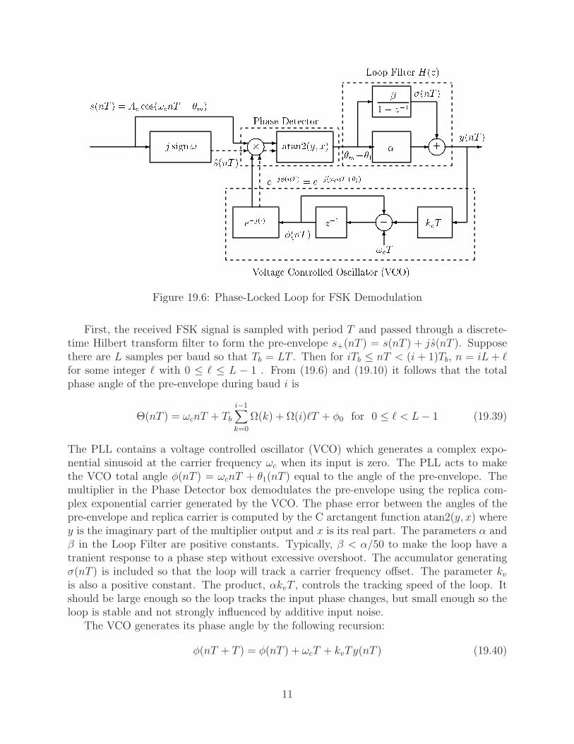
Figure 19.6: Phase-Locked Loop for FSK Demodulation

First, the received FSK signal is sampled with period T and passed through a discrete-time Hilbert transform filter to form the pre-envelope s+(nT ) = s(nT ) + js(nT ). Supposethere are L samples per baud so that Tb = LT . Then for iTb ≤ nT < (i + 1)Tb, n = iL + ℓfor some integer ℓ with 0 ≤ ℓ ≤ L − 1 . From (19.6) and (19.10) it follows that the totalphase angle of the pre-envelope during baud i is

Θ(nT ) = ωcnT + Tb

i−1∑

k=0

Ω(k) + Ω(i)ℓT + φ0 for 0 ≤ ℓ < L− 1 (19.39)

The PLL contains a voltage controlled oscillator (VCO) which generates a complex expo-nential sinusoid at the carrier frequency ωc when its input is zero. The PLL acts to makethe VCO total angle φ(nT ) = ωcnT + θ1(nT ) equal to the angle of the pre-envelope. Themultiplier in the Phase Detector box demodulates the pre-envelope using the replica com-plex exponential carrier generated by the VCO. The phase error between the angles of thepre-envelope and replica carrier is computed by the C arctangent function atan2(y, x) wherey is the imaginary part of the multiplier output and x is its real part. The parameters α andβ in the Loop Filter are positive constants. Typically, β < α/50 to make the loop have atranient response to a phase step without excessive overshoot. The accumulator generatingσ(nT ) is included so that the loop will track a carrier frequency offset. The parameter kvis also a positive constant. The product, αkvT , controls the tracking speed of the loop. Itshould be large enough so the loop tracks the input phase changes, but small enough so theloop is stable and not strongly influenced by additive input noise.

The VCO generates its phase angle by the following recursion:

φ(nT + T ) = φ(nT ) + ωcT + kvTy(nT ) (19.40)

11

Therefore

kvy(nT ) =φ(nT + T )− φ(nT )

T− ωc (19.41)

During baud i and assuming the loop is perfectly in lock so that Θ(nT ) = φ(nT ), substitutingΘ(nT ) given by (19.39) for φ(nT ) into (19.41) gives

kvy(nT ) =Θ(nT + T )−Θ(nT )

T− ωc = Ω(i) (19.42)

Therefore, the PLL is an FSK demodulator.When the loop is in lock and the phase error is small, atan2(x, y) can be closely approxi-

mated by the imaginary part of the complex multiplier output divided by Ac. The multiplieroutput is

[s(nT ) + js(nT )]e−jφ(nT ) = Acej[ωcnT+θm(nT )]e−jφ(nT ) = Ace

j[φm(nT )−θ1(nT )] (19.43)

and its imaginary part is

s(nT ) cosφ(nT )− s(nT ) sinφ(nT ) = Ac sin[φm(nT )− θ1(nT )] ≃ Ac[φm(nT )− θ1(nT )](19.44)

where Ac = |s(nT ) + js(nT )|. The imaginary part can be divided by the computed Ac orthis scaling can be accomplished by an automatic gain control (AGC) in the receiver or byadjusting the loop parameters. The loop gain in the PLL and, hence, its transient responsedepend on Ac if the approximation (19.44) is used, so this normalization by Ac is important.The atan2(y, x) function automatically does the normalization.

An example of the PLL behavior is shown in Figure 19.7 for a binary FSK input signal.The binary data input to the modulator was a PN sequence generated by a 23-stage feedbackshift register. The carrier frequency was 4 kHz, the frequency deviation was 200 Hz, and thebaud rate was 400 Hz. The output shows a segment where the input alternated between 0and 1 followed by a string of 1’s.

19.3.4 Optimum Noncoherent Detection by Tone Filters

The FM discriminator performs very poorly when the SNR is low or the FSK signal isdistorted, for example, by a speech compression codec in a cell phone because differentiationemphasizes noise. The phase-locked loop demodulator performs better than the discriminatorat low SNR but can have difficulty locking on to FSK signals that are present in short bursts.A better detector for these cases that uses “tone filters” is described in this section. Thisapproach does not use knowledge of the carrier phase and is called noncoherent detection.

A result in detection theory is that in the presence of additive white Gaussian noise thedetection strategy that is optimum in the sense of minimizing the symbol error probabilityfor symbol interval N is to compute the following statistics for the symbol interval and decidethat the frequency that was transmitted corresponds to the largest statistic2:

Ik(N) =

(N+1)Tb∫

NTb

s(t) cos(Λkt+ ǫ) dt

2

+

(N+1)Tb∫

NTb

s(t) sin(Λkt+ ǫ) dt

2

(19.45)

2J. M. Wozencraft and I. M. Jacobs, Principles of Communication Engineering, John Wiley & Sons, Inc.,1965, pp. 511–523.

12

24 26 28 30 32 34 36 38

−200

−150

−100

−50

0

50

100

150

200

Time in Bauds t / Tb

y(nT

) /(

2 π)

Figure 19.7: PLL Output with 1/T = 16000 Hz, kv = 1, αkvT = 0.2, and β = α/100

=

∣

∣

∣

∣

∣

∣

∣

(N+1)Tb∫

NTb

s(t)e−j(Λkt+ǫ) dt

∣

∣

∣

∣

∣

∣

∣

2

=

∣

∣

∣

∣

∣

∣

∣

(N+1)Tb∫

NTb

s(t)e−jΛkt dt

∣

∣

∣

∣

∣

∣

∣

2

for k = 0, . . . ,M−1(19.46)

where s(t) is the noise corrupted received signal and ǫ is a conveniently selected phaseangle. Notice that the statistics have the same value for every choice of ǫ. Remember thatΛk = ωc + Ωk = ωc + ωd[2k −M − 1] is the total tone frequency.

The statistic, Ik(N), can be computed in several ways. The receiver could implement(19.45) in the obvious way. It could have a set of M oscillators, each generating an inphasesine wave cos Λkt and a quadrature sine wave sinΛkt. Then it would multiply the input, s(t),by the sine waves, integrate the products over each baud, and form the sum of the squares ofthe inphase and quadrature integrator outputs for each tone frequency. The receiver wouldthen decide that the tone frequency corresponding to the largest statistic was the one thatwas transmitted for that baud.

The statistics can also be generated using a bank of filters. Let the impulse response of

13

the kth tone filter be

hk(t) =

ejΛkt for 0 ≤ t < Tb

0 elsewhere(19.47)

The output of this filter when the input is s(t) is

yk(t) =∫ t

t−Tb

s(τ)ejΛk(t−τ) dτ =∫ t

t−Tb

s(τ)e−jΛkτ dτ ejΛkt (19.48)

=∫ t

t−Tb

s(τ) cos[Λk(t− τ)] dτ + j∫ t

t−Tb

s(τ) sin[Λk(t− τ)] dτ (19.49)

Let t = (N+1)Tb which is at the start of symbol interval N+1 or the end of symbol intervalN . Then

|yk(NTb + Tb)|2 =

∣

∣

∣

∣

∣

∫ (N+1)Tb

NTb

s(τ)e−jΛkτ dτ

∣

∣

∣

∣

∣

2

(19.50)

which is the desired statistic Ik(N) given by (19.46).The frequency response of a tone filter is

Hk(ω) =∫ Tb

0ejΛkte−jωt dt =

1− e−j(ω−Λk)Tb

j(ω − Λk)= e−j(ω−Λk)Tb/2 Tb

sin[(ω − Λk)Tb/2]

(ω − Λk)Tb/2(19.51)

The magnitude of this function has a peak at the tone frequency Λk and zeros spaced atdistances that are integer multiples of ωb = 2π/Tb away from the peak. Thus, the tone filtersare bandpass filters with center frequencies equal to the M tone frequencies.

19.3.4.1 Discrete-Time Implementation

Discrete-time approximations to the statistics must be used in DSP implementations. Theintegrals can be approximated by sums. Suppose there are L samples per symbol so thatTb = LT . Then the last term on the right of (19.46) can be approximated by

Ik(N)/T 2 ≃ Dk(N) =

∣

∣

∣

∣

∣

∣

(N+1)L−1∑

ℓ=NL

s(ℓT )e−jΛkℓT

∣

∣

∣

∣

∣

∣

2

(19.52)

A discrete-time approximation to the tone filter is

hk(nT ) =

ejΛknT for n = 0, 1, . . . , L− 10 elsewhere

(19.53)

and the output of this filter is

yk(nT ) =n∑

ℓ=n−L+1

s(ℓT )ejΛk(n−ℓ)T = ejΛknTn∑

ℓ=n−L+1

s(ℓT )e−jΛkℓT (19.54)

Notice that each of the M tone filter impulse responses is convolved with the same set ofL samples s(ℓT )nℓ=n−L+1. Therefore, an efficient implementation in terms of minimummemory usage should have only one delay line containing these L samples.

14

The decision statistics for symbol interval N are obtained at the end of this interval byletting n = (N + 1)L− 1 in (19.54) to get

|yk[(N + 1)LT − T ]|2 =

∣

∣

∣

∣

∣

∣

ejΛk[(N+1)L−1]T(N+1)L−1∑

ℓ=NL

s(ℓT )e−jΛkℓT

∣

∣

∣

∣

∣

∣

2

= Dk(N) (19.55)

The frequency response for tone filter k is

Hk(ω) =L−1∑

n=0

ejΛknT e−jωnT = e−j(ω−Λk)(L−1)T/2 sin[(ω − Λk)LT/2]

sin[(ω − Λk)T/2](19.56)

The amplitude response of this filter has a peak of value L at the tone frequency Λk and zerosat frequencies Λk + p ωb in the interval 0 ≤ ω < ωs where p is an integer and ωb = 2π/Tb. Itrepeats periodically outside this interval as would be expected for the transform of a sampledsignal. This tone filter is a bandpass filter centered at the tone frequency Λk.

The block diagram of a receiver using tone filters is shown in Figure 19.8 for M = 4. Theboxes labelled “Complex BPF” are the tone filters. The solid line at the output of a box isthe real part of the output and the dotted line is the imaginary part. The boxes labelled| · | form the squared complex magnitudes of their inputs. These squared magnitudes arethe squared envelopes of the tone filter outputs. The squared envelopes are sampled at theend of each symbol period, the largest is found, and the corresponding frequency deviationis assumed to be the one that was actually transmitted. This decision is then mapped backto the corresponding bit pattern.

If the receiver has locked its local symbol clock frequency to that of the received signaland the phase for sampling at the end of a symbol has been determined, then the convolutionsum in (19.54) only has to be computed at the sampling times. In between sampling times,new samples must be shifted into the filter delay line but the output does not have to becomputed. In practice the clocks will continually drift and must be tracked. The blockdiagram indicates that the tone filter outputs are computed for each new input sample. Itwill be shown below how a signal for clock tracking can be derived from these signals.

19.3.4.2 Recursive Implementation of the Tone Filters

The tone filters can be efficiently implemented recursively when their outputs must be com-puted at every sampling time. To ensure stability of the recursion, the tone filter impulseresponses will be slightly modified to gk(nT ) = rnhk(nT ) where r is slightly less than 1. Thez-transform of a modified tone filter impulse response is

Gk(z) =L−1∑

n=0

rnejΛknT z−n =1− rLejΛkLT z−L

1− rejΛkT z−1(19.57)

The output of this modified tone filter can be computed as

yk(nT ) = s(nT )− rLejΛkLT s(nT − LT ) + rejΛkTyk(nT − T ) (19.58)

15

e2(nT ) HH

HH

HH

HH

-

-

-

-

-Ω(i)Largest

Select

-

-

-

-

-

-

-

-

-

-

-

-

????6

s(nT )

at Λ2

at Λ3

Complex BPF

Complex BPF

Complex BPF

v0,i(nT )

v0,r(nT )

v1,r(nT )

v2,r(n)

v3,r(nT )

v1,i(nT )

v2,i(nT )

v4,i(nT )

e0(nT )

at Λ1

Complex BPF

at Λ0

| · |2

| · |2

| · |2

| · |2

SymbolTiming

•

•

•

•

iTb

e3(nT )

e1(nT )

Figure 19.8: FSK Demodulator Using Tone Filters for M = 4

The real part of yk(nT ) is

vk,r(nT ) = ℜeyk(nT ) = s(nT )− rL cos(ΛkLT )s(nT − LT )

+ r cos(ΛkT )vk,r(nT − T )− r sin(ΛkT )vk,i(nT − T ) (19.59)

and the imaginary part is

vk,i(nT ) = ℑmyk(nT ) = −rL sin(ΛkLT )s(nT − LT )

+ r cos(ΛkT )vk,i(nT − T ) + r sin(ΛkT )vk,r(nT − T ) (19.60)

These last two equations are what could actually be implemented in a DSP since addi-tions and multiplications must operate on real quantities in a DSP. This filter structure issometimes called a “cross-coupled” implementation.

The quantities rL cos(ΛkLT ), rL sin(ΛkLT ), r cos(ΛkT ), and r sin(ΛkT ) can be precom-

puted. Then, computation of the real and imaginary outputs for the cross-coupled formrequires six real multiplications and five real additions for each n. Computation by directconvolution requires 2(L−1) real multiplications and 2(L−1) real additions for each n sincehk(0) = gk(0) = 1 and this is usually much larger than the computation required for thecross-coupled form.

The signal memory required for the cross-coupled form is an L + 1 word buffer to storethe real values s(ℓT )nℓ=n−L plus two locations to store vk,r(nT −T ) and vk,i(nT −T ). Thisis just slightly more than required by the direct convolution method.

19.3.4.3 Simplified Demodulator for Binary FSK

The demodulator structure can be simplified for binary (M = 2) FSK. A block diagramof the simplified demodulator is shown in Figure 19.9. The squared envelopes of the two

16

tone filter outputs are computed as before but now one is subtracted from the other. Thisdifference is passed through a lowpass filter to smooth it and eliminate some noise. Theslicer hard limits its input to a positive voltage A if its input is positive and to a negativevoltage −A if its input is negative. When no noise is present on the transmission channel, aslicer output of A indicates that the frequency deviation Ω1 was transmitted and an outputof −A indicates that Ω0 was transmitted during the symbol interval.

y(nT )

at Λ1

at Λ0

e1(nT )

e0(nT )

v(nT )Slicer

-

-

-

6

?

-

Upper

Lower

| · |2

| · |2

+

−

+s(nT )

Filter

Filter

Tone

Tone

- - -Lowpass

Filter

Figure 19.9: Simplified FSK Demodulator Using Tone Filters for M = 2

19.3.4.4 Generating a Symbol Clock Timing Signal

In a low noise environment and when the system filters are wideband, the symbol clock canbe tracked by locking to the sharp transitions in the demodulator output. This will not workin a high noise environment and when the system filters cause gradual transitions. One wayto generate a signal for clock tracking in this latter case is to form the sum, c(nT ), of the(

M2

)

= M(M − 1)/2 absolute values of the differences of the pairs of different tone filteroutput squared envelopes. In equation form

c(nT ) =∑

0≤i<j≤M−1

| ei(nT )− ej(nT )| (19.61)

The idea behind this signal is that during each symbol where the tone frequency changesfrom the one in the previous symbol, the tone filter output for the previous tone will ringdown and the tone filter output for the new tone will ring up, so the absolute value ofthe difference will show a transition. The tone filter envelopes can then be sampled at thepeaks of c(nT ), the largest envelope determined, and the result mapped back to a data bitsequence.

The presence of an FSK signal can be detected by monitoring the sum of the M squaredenvelopes

ρ(nT ) =M−1∑

k=0

ek(nT ) (19.62)

This sum indicates the power received in the tone filter pass bands. Detection of an FSKsignal can be declared when ρ(nT ) exceeds a threshold for one or more samples. The ter-mination of an FSK signal can be declared when the sum falls below a threshold. Thetermination threshold can be set below the detection threshold to allow hysteresis.

17

When the tone frequency is the same in adjacent symbols, the tone filter output envelopeswill not change and c(nT ) will not have a transition between the symbols. A symbol clocktracking algorithm based on c(nT ) would have to “flywheel” through the symbol intervalswhere c(nT ) has no transitions. A solution to this problem is to pass c(nT ) through abandpass filter centered at the symbol rate fb. A simple 2nd order bandpass filter with nullsat 0 and fs/2 Hz and a peak near fb Hz has the transfer function

H(z) = (1− r)1− z−2

1− 2z−1r cos(2πfb/fs) + r2z−2(19.63)

where fs is the sampling rate and r is a number close to but slightly less than 1. The closerr is to 1, the more narrow the filter bandwidth. Let c(nT ) be the filter input, y(nT ) thefilter output, and v(nT ) an internal filter signal. Then the filter output can be computedrecursively by the equations

v(nT ) = (1− r)c(nT ) + 2r cos(2πfb/fs)v(nT − T )− r2v(nT − 2T ) (19.64)

y(nT ) = v(nT )− v(nT − 2T ) (19.65)

This filter will “ring” at the symbol clock frequency. The receiver’s clock tracker can lock tothe positive zero crossings of this signal. The slope of the filter output y(nT ) is a maximum atthe zero crossings. Therefore, the zero crossings can be determined with significantly higheraccuracy than the peaks where the slope is zero. The peaks of the tone filter envelopes willoccur with some delay from these zero crossings depending on the filter parameters. Thetone filter squared envelopes should be sampled with this delay from the zero crossings. Thebandpass filter output will continue to oscillate at the symbol rate but will decay exponen-tially through intervals where the input is constant because of no tone frequency changes.By choosing r close enough to 1, the output will remain large enough during the intervalswith no transitions to still detect the positive zero crossings and allow the clock tracker toautomatically flywheel through these intervals.

An M = 4 FSK Example Using Tone Filters

Typical signals for an M = 4 FSK signal with fd = 200 Hz, fc = 4000 Hz, fb = 400 Hz, andfs = 16000 Hz and tone filter detection are shown in Figures 19.10, 19.11, 19.12, 19.13, and19.14. The tone frequencies are 3400, 3800, 4200, and 4600 Hz. For the tone filters r = 0.999and for the clock bandpass filter r = 0.998.

Figure 19.10 shows a small segment of the FSK signal. The tone frequency for symbolsduring normalized times 10 to 11 and 12 to 13 is 4600 Hz. The tone frequency during times11 to 12 and 13 to 14 is 3400 Hz. The varying amplitudes is an illusion created by connectingsamples of the signal taken at a 16000 Hz rate with straight lines.

Figure 19.11 shows the squared envelope e0(nT ) at the output of the 3400 Hz tone filter.Notice that the peaks occur at the integer normalized times.

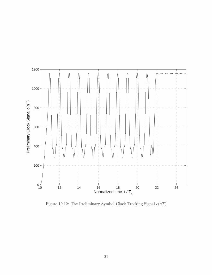
Figure 19.12 shows a segment of the preliminary clock signal c(nT ) computed as

c(nT ) = | e0(nT )− e1(nT )|+ | e0(nT )− e2(nT )|+ | e0(nT )− e3(nT )|

+ | e1(nT )− e2(nT )|+ | e1(nT )− e3(nT )|+ | e2(nT )− e3(nT )| (19.66)

18

10 10.5 11 11.5 12 12.5 13 13.5 14−1

−0.8

−0.6

−0.4

−0.2

0

0.2

0.4

0.6

0.8

1

Normalized time t / Tb

FS

K S

igna

l s(n

T)

Figure 19.10: Segment of the FSK Signal

The tone frequencies for symbols 10 through 21 alternate between 3400 and 4600 Hz creatingpeaks in c(nT ) each symbol as the envelopes of the corresponding two tone filters charge upand down. The tone frequency remains constant during symbols 22, 23, and 24, so there isno change in the tone filter output squared envelopes and c(nT ) had no transitions. Observethat the peaks occur at the integer normalized times which are exactly where the peaks ine0(nT ) occur in Figure 19.11. One could lock to the peaks in c(nT ) and sample the envelopesat the peak times but would have to “flywheel” through intervals when the tone frequencydoes not change.

Figure 19.13 shows the result when c(nT ) is passed through the bandpass filter centered atthe symbol clock frequency. This signal oscillates at the symbol clock frequency. Notice thatthe signal is exponentially damped between normalized times 22 and 30. This correspondsto an interval when c(nT ) has no transitions.

Figure 19.14 shows a segment of the preliminary clock signal, c(nT ), and the bandpassfiltered clock signal, y(nT ), superimposed on the same graph. The peaks of y(nT ) occur atalmost the same times as the peaks in c(nT ). The positive zero crossings of y(nT ) occur 1/4of a symbol before the peaks of c(nT ). A good clock tracker would lock to these zero crossingand the receiver would then sample the tone filter squared envelopes with a delay of 1/4 ofa symbol which corresponds to the peaks of c(nT ). The exact delay necessary depends on

19

12 14 16 18 20 22 240

50

100

150

200

250

300

350

400

Normalized time t / Tb

3400

Hz

Ton

e F

ilter

Squ

ared

Out

put E

nvel

ope

Figure 19.11: 3400 Hz Tone Filter Output Squared Envelope

the filter parameters.

20

10 12 14 16 18 20 22 240

200

400

600

800

1000

1200

Normalized time t / Tb

Pre

limin

ary

Clo

ck S

igna

l c(n

T)

Figure 19.12: The Preliminary Symbol Clock Tracking Signal c(nT )

21

16 18 20 22 24 26 28 30 32 34 36 38−300

−200

−100

0

100

200

300

Normalized time t / Tb

Ban

dpas

s F

ilter

ed P

relim

inar

y C

lock

Sig

nal y

(nT

)

Figure 19.13: The Signal c(nT ) Passed through a 2nd Order Bandpass Filter

22

19 19.5 20 20.5 21 21.5 22 22.5 23−300

−200

−100

0

100

200

300

Normalized time t / Tb

c(nT)/4y(nT)

Figure 19.14: Superimposed Preliminary and Bandpass Filtered Clock Signals

23

19.4 Symbol Error Probabilities for FSK Receivers

The problem of computing the symbol error probability for different types of FSK receiversis discussed extensively in Chapter 8 of Lucky, Salz, and Weldon3. The problem is verydifficult because of the nonlinear natures of the modulator and various receivers. Many ofthe results are approximations or require evaluation of complicated integrals by numericalintegration.

19.4.1 Orthogonal Signal Sets

One case where exact closed form results are know is when the transmitted symbols areorthogonal, they are corrupted by additive white Gaussian noise, and optimum noncoherentdetection by tone filters is used. Two continuous-time signals over the interval [t1, t2) withcomplex envelopes x1(t) and x2(t) are said to be orthogonal if

ρ =∫ t2

t1x1(t)x2(t) dt = 0 (19.67)

From (19.13) it follows that the complex envelopes of the FSK signal set during symbolperiod i where iTb ≤ t < (i+ 1)Tb are

xk(t) = Acejθm(iTb)ejωd[2k−(M−1)](t−iTb) for k = 0, . . . ,M − 1 (19.68)

For two distinct integers k1 and k2 in this set

ρ =∫ (i+1)Tb

iTb

xk1(t)xk2(t) dt = A2c

∫ (i+1)Tb

iTb

ej2ωd(k1−k2)(t−iTb) dt = A2c

∫ Tb

0ej2ωd(k1−k2)t dt

= A2c

ej2ωd(k1−k2)Tb − 1

j2ωd(k1 − k2)(19.69)

This integral will be zero if 2ωd(k1−k2)Tb = 2πℓ or h(k1−k2) = ℓ where ℓ is an integer. Thiswill be satisfied for all pairs of signals in the FSK signal set when the modulation index, h,is an integer.

An analogous property holds for the discrete-time FSK approximation. Assume there areL samples per symbol so that Tb = LT . The complex discrete-time envelopes during symbolinterval i where iTb ≤ nT < (i+ 1)Tb are

xk(nT ) = Acejθm(iTb)ejωd[2k−(M−1)](nT−iLT ) for k = 0, . . . ,M − 1 (19.70)

Then for two distinct integers k1 and k2 the correlation is

ρ =(i+1)L−1∑

n=iL

xk1(nT )xk2(nT ) = A2c

L−1∑

n=0

ej2ωd(k1−k2)nT = A2c

1− ej2ωd(k1−k2)LT

1− ej2ωd(k1−k2)T(19.71)

3R.W. Lucky, J. Salz, and E.J. Weldon, Principles of Data Communication, McGraw-Hill Book Company,1968

24

The correlation ρ will be zero if 2ωd(k1−k2)LT = 2ωd(k1−k2)Tb = 2πℓ where ℓ is an integerjust as in the continuous-time case. Therefore, all pairs of discrete-time FSK signals in theset will be orthogonal if h is an integer.

The energy transmitted during symbol period i is

E =∫ (i+1)Tb

iTb

s2(t) dt =1

2

∫ (i+1)Tb

iTb

|xk(t)|2 dt = A2

cTb/2 (19.72)

and the average power transmitted during this interval is S = E/Tb. Let the two-sided noisepower spectral density be N0/2. Then the symbol error probability is4

Pe =exp

(

−E

N0

)

M

M∑

i=2

(−1)i(

M

j

)

exp(

E

iN0

)

(19.73)

For binary FSK, i.e., M = 2, the symbol error probability is

Pe =1

2exp

(

−E

2N0

)

(19.74)

An upper bound for the symbol error probability for arbitrary M is

Pe ≤M − 1

2exp

(

−E

2N0

)

(19.75)

There are k = log2 M bits per symbol. For orthogonal signal sets, all symbol errors areequally likely, so all bit-error patterns in a block of k transmitted bits assigned to a symbolare equally likely. Based on this observation, Viterbi5 shows that the bit error probability isrelated to the symbol error probability by the formula

Pb =2k−1

2k − 1Pe (19.76)

19.5 Experiments for Continuous-Phase FSK

For these experiments you will exploreM = 2 andM = 4 continuous-phase FSK transmittersand receivers. For all these experiments use the following parameters: carrier frequencyfc = 4000 Hz, frequency deviation fd = 200 Hz, symbol rate fb = 400 Hz, sampling frequencyfs = 16000 samples per second, and p(t) is the rectangular pulse given by (19.4). Initializethe TMS320C6713 DSK as usual.

19.5.1 Theoretical FSK Spectra

Write a MATLAB program or use any other favorite programming language to compute thepower spectral density for an FSK signal with arbitrary M , fc, fd, and fb using (19.27).Then plot the spectra for M = 2 and M = 4 vs. the normalized frequency (ω − ωc)/ωb forthe parameters specified for these experiments. Experiment with other parameters also.

4Andrew J. Viterbi, Principles of Coherent Communication, McGraw-Hill, 1966, p. 247.5Andrew J. Viterbi, Principles of Coherent Communication, McGraw-Hill, 1966, p. 226.

25

19.5.2 Making FSK Transmitters

Write programs for the TMS320C6713 DSK to implement continuous-phase FSK transmit-ters for M = 2 and M = 4. Write the output samples to the left codec output channel. Youwill be using these transmitters as FSK signal sources for your receivers.

19.5.2.1 Initial Handshaking Sequence

To help the receivers detect the presence of an FSK signal and lock to the transmitter’ssymbol clock, make your transmitter send the following signal sequence:

1. First send 0.25 seconds of silence, that is, send 0 volts for 0.25 seconds. This willallow your receiver to skip over any initial transient that occurs when the transmitterprogram is loaded and started.

2. Then for M = 2 send 25 symbols alternating each symbol between f0 = 3800 andf1 = 4200 Hz tones. This will allow the receivers to detect the FSK signal and lockon to the symbol clock. For M = 4 send 25 symbols alternating each symbol betweenf0 = 3400 and f3 = 4600 Hz.

3. Suppose the frequencies of the last few symbols of the alternating sequence for M = 2were · · · , f0, f1, f0. Next send an alternating frequency sequence for 10 symbols butwith the alternation reversed. That is send f0, f1, f0, f1, f0, f1, f0, f1, f0, f1. Your re-ceiver can detect this change in the alternations and use it as a timing mark to deter-mine when actual data will start.

For the M = 4 transmitter change to alternating between f1 = 3800 and f2 = 4200 Hzfor 10 symbols. Again, this change can be used as a timing mark.

19.5.2.2 Simulating Random Customer Data

After the alternations, begin transmitting “customer” data continuously. Simulate this databy using a 23 stage PN sequence generator as discussed in Chapter 9. Use the connectionpolynomial h(D) = 1+D18+D23 so the data bit sequence, d(n), is generated by the recursion

d(n) = d(n− 18)⊕ d(n− 23) (19.77)

where “⊕” in the recursion is modulo 2 addition, that is, the exclusive-or operation. Initializethe PN sequence generator shift register to some non-zero state.

For M = 2, shift the PN generator once to get a new data bit d(n) which will be a 0 or1. Map this bit to the tone frequency Λ(n) = ωc + ωd[2d(n)− 1].

For M = 4, shift the register twice to get a pair of bits [d1(n), d0(n)]. Consider this bitpair to be the integer k(n) = 2d1(n) + d0(n) which can be 0, 1, 2, or 3. Map this bit pair tothe tone frequency Λ(n) = ωc + ωd[2k(n)− 3].

26

19.5.2.3 Experimentally Measure the FSK Power Spectral Density

Measure the power spectral density of the transmitted FSK signals for M = 2 and 4 after theinitial handshaking sequence when random customer data is being transmitted. If you madethe spectrum analyzer for Chapter 4, run it on one station and connect your transmitterto it. You can use a commercial spectrum analyzer if it is available. Otherwise collect anarray of transmitted samples, write them to a file on the PC, and use MATLAB’s SignalProcessing Toolbox function pwelch( ). Compare your measured spectra with the theoreticalones you computed.

19.5.3 Making a Receiver Using an Exact Frequency Discrimina-tor

Make a receiver using the exact frequency discriminator shown in Figure 19.4 for M = 2.Connect the transmitter from another station to your receiver. There are RCA-to-RCAbarrel connectors in the cabinet to connect RCA to mini-stereo cables together. First leaveyour transmitter off and turn on your receiver. When the receiver is running, turn on yourtransmitter. Your receiver program should do the following:

1. The receiver should detect the absence or presence of an input FSK signal by monitor-ing the received signal power. The power can be calculated by doing a running averageof the squared input samples over several symbols. You can also try a single poleexponential averager. The receiver should assume that no FSK input signal is presentwhen this power is small and sit in a loop checking for the presence of an input signal.When the measured power crosses a threshold, the receiver can start the discriminatorand symbol clock tracking algorithm. You should predetermine a good threshold basedon your knowledge of the transmitter amplitude and system gains. You can do thisexperimentally by observing the received power when the transmitter is running.

2. The receiver should continue to monitor the input signal power and detect when thesignal is gone and go into a loop looking for the return of a signal.

3. Start your discriminator and symbol clock tracker once an input signal is detected.Monitor the tone frequency alternations and look for the alternation switch. Countfor 10 symbols after the switch and begin detecting the tone frequencies resulting fromthe input customer data.

4. Send the output samples of the discriminator to the left codec channel. Send a signalto the right codec output channel that is a square wave at the symbol clock frequencyto use for synching the oscilloscope. You can do this by sending a positive value for 20samples at the start of a symbol followed by its negative value for the next 20 samples.Observe the result and take a picture of a single trace on the oscilloscope screen toshow a typical output of the discriminator. Alternatively, you can capture an array ofdiscriminator output samples with Code Composer or use fprintf(·) to write the arrayto a PC file and plot the output file with your favorite plotting program.

27

If you allow the oscilloscope to run freely, you will see multiple traces synchronizedwith the symbol clock overlapped on the screen. This type of display is called an “eyepattern” in the communications industry. At the end of each symbol you should seetwo distinct equal and opposite levels and the eye is said to be open. The eye patterncan be used as a diagnostic tool. Noise and system problems cause the eye to be lessopen. Decision error will occur if the eye is closed.

5. Map the detected tone frequency sequence back into a bit sequence d(n).

6. Check that the received bit stream is the same as the transmitted one. Your receivershould have a 24-stage shift register that contains d(n), d(n − 1), . . . , d(n − 23). Youcan check for errors by checking that

d(n)⊕ d(n− 18)⊕ d(n− 23) = 0

for all n except for an initial burst of 1’s when the shift register is filling up. If youinitialize the state of the register to the initial state of the transmitter register theresult should be all 0’s if you have detected the starting time of the customer datacorrectly.

19.5.3.1 Running a Bit-Error Rate Test (BERT)

A measure of the quality of a digital transmission scheme is its bit-error rate performance inthe presence of additive noise. Once your receiver is working correctly with noiseless receivedFSK signals, perform a bit-error rate test as follows:

1. Generate zero-mean Gaussian noise samples in the DSP with some variance σ2 andadd them to the received signal samples. Implement a power meter in your receiverprogram to measure the power of the FSK input samples, say P . Compute the SNR= 10 log10(P/σ

2) dB.

2. Your receiver should have a replica of the PN sequence generator in the transmitter.You should synchronize the state of the local PN generator to that of the transmitterso it’s output sequence will be in phase with the received one.

3. Start your BERT test with a very high SNR so few errors will occur. Check if each bitestimated by the receiver is the same as the transmitted one and count any bit errorsfor a number of bits sufficient to give a good estimate of the bit-error probability. Theestimated bit-error rate is BER = (the number of errors in the observed sequence ofdetected bits)/(the number of observed detected bits). The number of observed bitsshould be at least 10 times the bit-error rate to get an estimate with good accuracy.The variance of this estimator decreases inversely with the number of observed bits.

4. Decrease the SNR in steps of 0.25 dB and measure the bit-error rate for each SNR. Con-tinue decreasing the SNR until you can no longer synchronize the replica PN generatorwith the transmitter’s generator.

28

5. Plot the bit-error rate vs. SNR. The bit-error rate should be plotted on a logarithmicscale and SNR in dB on a linear scale. This kind of plot is known as a “waterfall curve”in the communications industry.

19.5.4 Making a Receiver Using an Approximate Frequency Dis-criminator

Repeat the tasks for the exact frequency discriminator in Section 19.5.3 for the approximatefrequency discriminator of Section 19.3.2.

19.5.5 Making a Receiver Using a Phase-Locked Loop

Make a receiver using the phase-locked loop described in Section 19.3.3 for M = 2. Test yourreceiver by following the steps in Section 19.5.3. Compare the bit-error rate performance ofthis receiver with the discriminator receiver.

19.5.6 Making a Receiver Using Tone Filters

19.5.6.1 M = 4 Tone Filter Receiver

Make a receiver using tone filters for M = 4 FSK. Implement the method for generating asymbol clock tracking signal described in Section 19.3.4.4. Use the sum of the tone filteroutput squared envelopes, ρ(nT ) given by (19.62), to detect the presence or absence of areceived FSK signal. Test your receiver by following the steps for the exact discriminatorin Section 19.5.3. In addition, send the squared envelope at the output of one of the tonefilters to one output channel of the codec, send the output of the 2nd order bandpass symbolclock tone generation filter to the other channel to use as a synch signal, observe them onthe oscilloscope, and record the display. Also send the preliminary clock tracking signal tothe oscilloscope and record the result. Compare your measured bit-error rate curve withthe theoretical bit error probability curve given by (19.76). Also compare the bit-error rateperformance of this receiver to the others.

19.5.6.2 Simplified M = 2 Tone Filter Receiver

Make and test the simplified binary tone filter receiver described in Section 19.3.4.3. Measureand plot the bit-error rate vs. SNR and compare it with the theoretical curve.

29