Addressing missing values in Credit Scoring · Missing data theory (Rubin, 1976) involves two sets...

1

Addressing missing values in Credit Scoring

Haoye Liang, Jake Ansell and Meng Ma

University of Edinburgh Business School

ABSTRACT

Credit scoring is beset with issue of missing values whether it be for retail or Small and Medium-Sized Enterprises

(SMEs). Historically in Credit Scoring, the approach has been to employ Weights of Evidence (WoE). Ma (2016)

suggested using a continuous method related to WoE. This allowed the use of generalized additive model (GAM).

Subsequently, Liang (2018) has applied Multiple imputation by chain equations (MICE) as an approach to impute

the missing values. Partially the differences in approach depend on one’s belief about nature of the missing values.

WoE is closer to assuming that values are Missing Not At Random, which Meng took a related approach allowing

GAM. MICE, on the other hand, assumes Missing At Random or Missing Completely At Random. In this paper,

we explore the effect of applying these different approaches on GAM. It illustrates that these approaches yield

different solutions not only in coefficient estimation but also in models built. From a regulatory point of view, this

raises a question about whether more thought is required for modelling into the future.

1. INTRODUCTION

Datasets are often partially observed in the real world. Hence, for analysis not all the intended data can be obtained

on all the subject especially for longitudinal or cross-sectional studies. Graham (2009) indicates that there can be

significant effect on derived models due to missing values across all areas of study. Discounting variables is an

inefficient use of the data (Peugh and Enders, 2004; Wood et al., 2004; Jeličić et al., 2009), particularly in the era

of big data. Wilkinson (1999) has warned that list-wise deletion is the worst methods available for practical

applications and others have expressed the disadvantage of such approaches (Graham, 2009; Little and Rubin,

2014). Therefore, alternative approaches are necessary; imputation, regression or use of dummy variables. Little

and Rubin (1987) and Little (1992) highlight the bias becomes an issue if reason for missing values is not

understood and as such may lead to invalid conclusions being made.

2. MISSING DATA MECHANISMS

In the handling of the missing value, it is necessary to identify the mechanism of missing in the employed data

since the performance of missing data techniques strongly depends on the mechanism that generated the missing

values. Rubin (1976) established a theoretical framework for missing data problem in the form of three

mechanisms, which bases on the probability of missingness, namely: missing complete at random (MCAR),

missing at random (MAR), and missing not at random (MNAR) respectively. The mechanism can be interpreted

as a probability distribution for the missing data. The result of this evaluation is significant since it limits the

possible approaches of dealing with the missing data in further analysis. The crucial role of the mechanisms in the

analysis of data with missing values was largely ignored until the concept was formalized in the way of treating

the missing data indicators as random variables and assigning them a distribution (Little and Rubin, 2014).

2

Let Y = (yij) denote an (n×T) data matrix without missing values, with ith row yi = (yi1,…, yiT) where yij is the

value of variable Yj for observation i. Rubin (1976) proposed that missingness is a variable that has a probability

distribution, and defined missing data indicator matrix R = rij, such that rij = 1 if yij is missing and rij = 0 if yij

is not missing, and this R matrix has the same size as the data matrix (matrix Y). R could be analysed by

researchers according to the probability models. The complete data (Ycom) can be divided into an observed (Yobs)

and a missing part (Ymis):

Ycom = Yobs + Ymis, (Yobs ∩ Ymis = ∅),

where ∅ are a set of unknown parameters that describe the relationship between R and the data.

If the probability of missing data on a variable Y depends only on the component Yobs but not on Ymis, that is, if

P(R |Ycom) = P(R |Yobs , ∅)

the data are defined as MAR where R takes on a value of zero or one depending on Yobs (Schafer and Graham,

2002). MCAR is a stronger assumption than MAR, which is that the probability of missing data on a variable Y

neither depends on Yobs nor Ymis. Missingness is completely unrelated to the data. That is

P(R |Ycom) = P(R |∅)

The probability of MCAR data is constant. MCAR data is rare since it is likely missing values are dependent on

other variables. In this case deletion method is unlikely to be biased, but this is not recommended because of

information loss. Incorrectly assuming MCAR assumption may lead to bias.

Finally, the mechanism is called MNAR if the probability of missing data on a variable Y can depend on other

variables (i.e., Yobs) as well as on the unobserved underlying values of Y itself (i.e., Ymis) (Enders, 2010). That is

P(R |Ycom) = P(R |Yobs, Ymis, ∅)

The MNAR assumption can be problematic to work with as the factors that influence Ymis are often difficult to

study.

MAR is commonly assumed for imputation methods as it does not carry the risk of MCAR misspecification and

the complexity of MNAR (Enders, 2010). Obviously it is possible to assume a pattern for missing such as

hierarchical, but it is probably that any pattern is arbitrary (Horton and Kleinman, 2007). Whilst MCAR can be

tested, neither MAR or MNAR can be, though, if MAR is assumed then it does not necessarily cause serious

consequences (Schafer and Graham, 2002). In case of SMEs one is unlikely to know the reason for missing, but

it is frequently assumed that it is either directly or indirectly correlated with the ‘bad’ performance of SMEs. In

other cases variables are not necessarily reported since they are not required by regulation. For example Firm Size

is a variable where Small Enterprises are not obligated to provide information in the same ways as Medium or

Large Enterprises, (Gov, 2018).

Missing data theory (Rubin, 1976) involves two sets of parameters: the parameters that have no missing data and

the parameters that describe the probability of missing data (i.e., ø). Given researchers rarely know why the data

are missing, then ø cannot be estimated with any certainty. Rubin’s theory clarified the conditions needed in order

to accurately estimate the parameters of interest without knowing the missing data distribution (i.e., ø). Rubin

3

showed that likelihood-based analyses such Maximum Likelihood Estimation (ML) and Multiple Imputation (MI)

do not require information about ø if the data are MCAR or MAR (Little and Rubin, 1987; Rubin, 1987a). Hence

MAR or MCAR mechanisms are described as ignorable missingness. Care has to be taken though dependent on

the missing data mechanism (Allison, 2000; Schafer, 2003). Practically, MI ensures obtaining accurate estimates

in a broader range of circumstances than simply deletion, even in cases where 50% or more data are missing

(Enders, 2010).

3. SMEs Data

The data in this study contains over 2 million SMEs recorded, but also covers 79 explanatory variables for the

SMEs. They cover the following aspects of a SME:

1. General information: such as their legal form, location information, 1992’s Section of Industry

Classification (SIC), No. of employees, age of company and so on.

2. Directors’ information: No. of directors in total and other general director’s information, management

ability not included.

3. Previous relevant credit history: such as DBT, judgement and previous searches information

4. Accounting information: all the commonly used financial ratios.

As seen from Table 1, both Start-ups and Non-Start-ups SMEs have three predictive variables with over 70%

missing observations, especially, time since last derogatory data item (months) with 96.69%. Hence, some

variables cannot be included whatever method is used. In order to ensure a stable and consistent analysis results,

it is necessary to use the same set of predictors over the years. It is reasonable to remove the effect that only are

significant for a specific year.

This paper employs WoE to transform variables, though, for MICE imputed do not use WoE transformation. Then

stepwise logistic regression is used for variable selection with only positive coefficient with confidence level 95%

for each year since negative coefficient would imply collinearity. In order to obtain the same set of predictive

variables, only those variables that are significant for at least three years, see Table 2. Different imputed methods

bring various predictive variables.

4. METHODOLOGY

This will detail the different approaches that have been taken to dealing with missing values within Credit Scoring;

Weights of Evidence (WoE) and related continuous approaches as well as describing method referred to as MICE.

4.1 Weight of Evidence (WoE)

The standard approach to dealing with missing values is WoE, it developed from Good’s concept of Information,

see Thomas () for full details. The approach starts for a variable by splitting the observed data into intervals and

including a category for missing values. This is referred to as coarse classifying. For the WoEi for the ith interval

of a variable is the log of the good/bad ratio of an interval is compared to the log whole data good/bad ratio for

the variable as:

4

WoEi = ln (Ni

Pi) − ln (

∑ Ni

∑ Pi)

Intervals with similar WoEi are combined. Usually the analyst will be look for up to 10 categories by this method.

The transformation is generally not linear but monotonic related to the bad rate. The model is fitted using WoE

values.

Table 1 Table Missing rates (%)

Variables Start-ups Non-Start-ups

2007 2008 2009 2010 2007 2008 2009 2010

Legal form 0 0 0 0 0.21 0.07 0.01 0.03

Company is subsidiary 0 0 0 0 - - - -

Parent company – derog details - - - - 0 0 0 0

1992 SIC code 58.39 60.2 58.5 60.9 3.5 3.6 4.3 3.6

Region 1.51 1.4 1.39 1.41 2.78 2.52 2.05 2.33

Proportion of current directors to

previous directors in the last year 81.5 85.5 87.9 88.8 93.8 94.1 95.5 92.5

No. Of ‘current’ directors - - - - 2.12 1.98 1.81 1.9

Oldest age of current directors/

proprietors supplied (years) 15.46 9.36 3.38 1.41 - - - -

Number of directors holding shares 0.72 0.64 0.84 0.6 - - - -

Pp worst (company DBT - industry DBT)

in the last 12 months - - - - 66.8 69.3 65.3 66.9

Total value of judgements in the last 12

months 0 0 0 0 0 0 0 0

Number of previous searches (last 12m) 0 0 0 0 0 0 0 0

Time since last derogatory data item

(months) 96.7 95.0 90.2 92.1 96.4 93.7 90 86.8

Lateness of accounts 0.5 0.5 0.5 0.6 1.7 1.6 1.4 1.5

Time since last annual return 57 56.9 52.8 56.4 2.7 2.4 2.9 2.4

Total assets 79.1 80.2 74.3 74.9 - - - -

Total fixed assets as a percentage of total

assets - - - - 3.75 4.33 4.69 4.75

Debt gearing (%) - - - - 92.0 91.9 94.2 91.7

Percentage change in shareholders’ funds - - - - 8.1 8.7 8.8 8.7

Notes: -: Not report the missing rate, 0: no missing values

5

Table 2 Independent variable reference for Start-ups and Non-Start-ups

Variables Selections Format Type

Sta

rt-u

ps

Legal Form MA &MICE Character General information

Company is Subsidiary MA Character General information

1992 SIC Code MA Character General information

Region MA &MICE Character General information

Proportion Of Current Directors To Previous

Directors In The Last Year

MA &MICE Numerical Directors information

Oldest Age Of Current Directors/Proprietors

supplied (Years)

MA &MICE Numerical Directors information

Number Of Directors Holding Shares MA &MICE Numerical Directors information

Total Value Of Judgements In The Last 12

Months

MA &MICE Numerical Payment and credit records

Number Of Previous Searches (last 12m) MA Numerical Payment and credit records

Time since last derogatory data item (months) MA &MICE Numerical Payment and credit records

Lateness Of Accounts MA &MICE Numerical Financial statement

Time Since Last Annual Return MA &MICE Numerical Financial statement

Total Assets MA &MICE Numerical Financial statement

Non-S

tart

-ups

Legal Form MA&MICE Character General information

Parent Company – derog details MA Character General information

1992 SIC Code MA Character General information

Region MA&MICE Character General information

No. Of ‘Current’ Directors MA&MICE Numerical Directors information

Proportion Of Current Directors To Previous

Directors In The Last Year

MA Numerical Directors information

PP Worst (Company DBT - Industry DBT) In

The Last 12 Months

MA&MICE Numerical Payment and credit records

Total Value Of Judgements In The Last 12

Months

MA&MICE Numerical Payment and credit records

Number Of Previous Searches (last 12m) MA Numerical Payment and credit records

Time since last derogatory data item (months) MA&MICE Numerical Payment and credit records

Lateness Of Accounts MA&MICE Numerical Financial statement

Time Since Last Annual Return MA&MICE Numerical Financial statement

Total Fixed Assets As A Percentage Of Total

Assets

MA&MICE Numerical Financial statement

Debt Gearing (%) MA Numerical Financial statement

Percentage Change In Shareholders Funds MA Numerical Financial statement

Percentage Change In Total Assets MA Numerical Financial statement

MA: selected by moving average; MICE: selected by multiple imputation by chained equations

6

4.2 Moving Average

WoE reorders the data according to the good/bad rate, but this can be hard to interpret when using some models.

It also renders continuous variables into discrete, though, then it is usually treated as continuous. The approach

taken by Meng (2016) tries to preserve variable values whilst including missing values as a specific value. It does

this by matching the missing value to an observed value. The single imputation used assumes that missing value

does not occur at random. A simple approach is to smooth the good rate of non-missing values and compare the

good rate of the missing value to the smooth curve. There are many ways to smooth data, the simplest would be

a moving average (MAi), defined as：

MAi =gi−n⋯+gi+⋯+gi+n

n,

where n is an appropriate integer and gi = 1 if ith value is good and 0 if ith value is bad.

Obviously, this makes sense for data which is at lease ordinal.

If a given value j is found to have the same performance as the missing category (MG):

MG = MAj

Else if

MG ≠ MAi for i = 1, 2, … , N

then

if MG − MAj = min|MG − MAi| for i = 1, 2, … , N

4.3 Multiple imputation of chained equations

Regarding Multiple imputation of chained equations (MICE), it is a special application of multiple imputation

(MI) technique (Raghunathan et al., 2001; Van Buuren, 2007). MI has been used in large datasets with thousands

of observations and hundreds of variables (He et al., 2010). It operates under the assumption that the given

variables used in the imputation procedure are missing data are miss at random (MAR) or missing complete at

random (MCAR). Implementing MICE when data are not MAR could result in biased estimates. In the MICE

procedures, a series of regression models are performed and each variable with missing data is modelled according

to its variable type. For example, binary variables can be imputed by logistic regression while continuous variables

can be imputed by linear regression.

4.3.1 MICE steps

MICE can be summarized in three stages: imputation, analysis and pooling, see Figure 1. The first step is to create

m sets of completed data by replacing each missing value with m imputed values. The second phase consists of

using standard statistical methods for separate analysis of each completed dataset as if it were a “real” completely

observed dataset. The third step is the pooling step where the results from m analyses are combined to form the

final result. This technique has become one of the most advocated methods for handling missing data.

7

Figure 1: Overview of the MI procedure (creating m imputed dataset)

(Azur et al., 2011) describes the process in 7 steps which can be performed separately. Rubin’s rules highlight

that the imputation and analysis stages conditioned on the same set of observed data. This implies that all variables

included in the analysis stage should also include in the imputation stage, otherwise biased estimates would be

produced.

4.3.2 Combining Rules

Rubin (1987a) proposed a series of rules to describe the combination of a single inference of multiple sets of

parameter estimates and standard errors after the generation of a number of imputed datasets, and these rules also

known as Rubin’s Rules. MI parameter estimate is the arithmetic average of the m complete-data estimates, which

mathematically is:

θ̅ =1

m∑ θ̂i

m

i=1

where θ̂i is a parameter estimate from imputed dataset i and θ̅ is the pooled estimate. It should be mentioned that

the foundation of MI is the Bayesian framework, but the pooled point estimate is valid for both a Bayesian and

frequentist approach. On the one hand, θ̅ is the mean of the posterior distribution, on the other hand, θ̅ is a point

estimate of the fixed population parameter (Rubin, 1987a) .

Pooling standard errors need to compute two components: within-imputation variance, and between-imputation

variance. Within-imputation variance estimates the sampling variability that we would have expected had there

been no missing data. The formula is given by VW =1

m∑ SEi

2mi=1 , where VW denotes the within-imputation

variance, and SEi2 is the squared standard error from imputed dataset i. This part is also simply the arithmetic

mean of the sampling variance from each dataset. Between-imputation variance quantifies variation in the

parameter values caused by missing data, as follows:

VB =1

m−1∑ (θ̂i − θ̅)

2mi=1 ,

where VB denotes the between–imputation variance, θ̂i is the parameter estimate from imputed

dataset i and θ̅ is the average point estimate of parameter estimate from the previous equation.

Incomplete data Imputation (m) Analysis Pooling

8

Finally, the total sampling variance is a sum of the previous two components with an additional

source of sampling variance, as follows:

VT = VW + VB +VB

m

where VT denotes the total sampling variance. The additional source (VB

m) represents the sampling error associated

with the extra variance caused by the fact that coefficient estimates are based on finite m. It is used as a correction

factor for using a specific number of imputations. When the number of imputation tends to infinity (VT = VW +

VB), the parameter estimate is more accuracy (Enders, 2010). Standard error is the square root of the total sampling

variance, as follows:

SE = √VT = √VW + VB +VB

m

4.3.3 Imputation diagnostic measure

The within-imputation variable, between-imputation, and the total variance define two useful diagnostic measure,

the fraction of missing information and the relative increase in variance due to nonresponse. Fraction of missing

information (FMI) estimates the missing data’s influence on the sampling variance of a parameter estimate. It is

estimated based on the percentage missing for a particular variable and how correlated this variable is with other

variables in the imputation model. Allison (2001) stated the FMI represents “how much information is lost about

each coefficient because of missing data”. Typically FMI is lower than the missing data rate, particularly when

the variables in the imputation model are predictive of the missing data (Longford, 2006; Enders, 2010). The FMI

formula is given below:

FMI ≈VB +

VB

mVT

The interpretation is similar to an R-squared. For example, an FMI of 0.15 implies that 15% of the total sampling

variance is because of missing data. Provided that a variable with large proportion of missing values, the smaller

FMI is, the more imputations are needed. The larger the number of imputations, the more precise the parameter

estimates will be. The accuracy of the estimate of FMI increases as the number imputation increases because

variance estimates stabilize with larger numbers imputations (Enders, 2010). A high FMI can indicate a

problematic variable as high rates of missing information tend to converge slowly, so that one should consider

increasing the number of imputations. A good rule of thumb is to set the number imputations (at least) equal the

highest FMI percentage.

4.3.4 Number of imputations

Historically, the recommendation for the number of imputation was three to five imputed datasets, which based

on the relative efficiency formula derived from RR (Rubin, 1987b). The relative efficiency (RE) of an imputation

measures how well the true population parameters are estimated and is related to both the amount of missing

information as well as the number of imputations performed. The formula is given below:

RE = (1 +FMI

m)−1

9

where m is the number of imputation and FMI is fraction of missing information. RE is an estimate of the

efficiency relative to performing an infinite number of imputations (m). The RE can be achieve with relative low

number of imputations. Yet more recently, the larger number of imputations are often recommended because of

the rapidly developed computing power and practical used for researchers. Schafer and Graham (2002) found that

20 imputations can effectively perform better estimates by removing noise from other statistical summarizes (e.g.,

significant levels or probability values). Graham et al. (2007) approached the problem in terms of loss of power

for hypothesis testing. Based on simulations and a willingness to tolerate up to a 1 per cent loss of power, they

recommended 20 imputations for 10% to 30% missing information, and 40 imputations for 50% missing

information. A larger number of imputations may also allow hypothesis tests with less restrictive assumptions

(i.e., that do not assume equal fractions of missing information for all coefficients). Allison (2012) indicated other

factors, such as standard error estimates, confidence intervals, and p-values need to be considered. One of the

critical components of Rubin’s standard error formula for MI is the variance of each parameter estimate across

the multiple datasets. With so few observations (datasets), it should not be surprising that standard error estimates

can be very unstable. Pan et al. (2014) pointed out that a small number of imputations may not be enough to obtain

a statistically reliable variance estimate. (Bodner, 2008) and Royston et al. (2011) by different approaches suggest

a rule of thumb: the number of imputations should be slightly higher to the percentage of cases that are incomplete.

Obviously, for any specific dataset the number of imputations might need to be higher and further work is required.

4.3.5 Non-normally distributed variables

Another uncertainty of MICE is specifying the imputation model correctly especially for non-normally distributed

variables. Non-normally distributed variables can be skewed, on limited-range or semi-continuous variables,

which consist of a large proportion of responses with point masses that are fixed at some value and a continuous

distribution among the remaining responses (Vink et al., 2014). Hence there is strong possibility of bias, von

Hippel (2013). Therefore, some researchers suggested to transform skewed variables to better approximate

normality variables (Schafer and Olsen, 1998; Allison, 2001; Raghunathan et al., 2001; Schafer and Graham,

2002). (Lee and Carlin, 2010) suggest using a de-skewing transformation, but for positively skewed when the

imputed values are transformed back, the imputed values can have very large outlying values (von Hippel, 2013).

Besides, the transformation does not yield normally distributed variable for both limited-range and semi-

continuous data (White et al., 2011).

Predictive mean matching (PMM) regression can be used when for a continuous variable, especially for semi-

continuous variable. In this approach imputed values are sampled only from the observed values of the variable

by matching predicted values as closely as possible, and it is free of distributional assumptions.

PMM tends to preserve the distributions of the original data. These properties generally appeal to applied

researchers, but it is undesirable when the sample size is small since only a small range of imputed values is

available (Heitjan and Little, 1991; Schenker and Taylor, 1996). PMM calculates the predicted value using a

regression model and picks the closest elements to the predicted value (by Euclidean distance). These chosen

elements are called the donor pool (the observations potentially available for matching predictions), and the final

value is chosen at random from this donor pool. The number in the donor pool is by default set to 5 in MICE (R

packages). Thus the imputed value is an observed value whose prediction with the observed data closely matches

10

the perturbed prediction (White et al., 2011). Vink et al. (2014) conclude that predictive mean matching

performance is the only method that yields plausible imputations and preserves the original data distributions. If

plausible values are necessary, this is a better choice than using bounds or rounding values produced from

regression. Lazure (2017) compared five methods and showed that PMM under MICE has better performance in

handling missing data.

4.4 Logistic regression

Logistic regression (Cox, 1958) is the classical statistical techniques for credit risk modelling because of its ability

to model binary classification problem (Andreeva et al., 2016). Given its strong theoretical support, it gives rise

directly to an additive log odds score which is a weighted linear sum of attribute values (Thomas, 2009). As a

standard benchmark, newly developed classifier algorithms compare classification performance against it (Lee et

al., 2002; Ong et al., 2005; Bellotti and Crook, 2009; Nehrebecka, 2018). The logistic regression model is given

by the equation:

P(yi = 1|x) =eβ0+β1x1+⋯+βpxp

1 + eβ0+β1x1+⋯+βpxp

where β0 is the intercept and β1, …, βp is coefficients of variable x1, …, xp.

Independent variables transformed by WoE are particularly well suited for logistic regression. The link between

logistic regression and weight of evidence is provided in the following equation. Besides, they also have ties to

well-known naive Bayes classifier, given by (Friedman et al., 2001):

log (P(yi = 1|x1, … , xp)

P(yi = 0|x1, … , xp)) = log (

P(Y=1)

p(Y=0)) + ∑ (

f(xn|Y=1)

f(xn|Y=0))n

i=1 .

4.5 Generalized additive models (GAMs)

Generalized additive models (GAMs) proposed by (Hastie and Tibshirani, 1986) is a flexible statistical approach

which can identify and capture non-linear regression effects, which allows the closer fit to the real relationship

between the variables. GAM automatically fits a non-linear function for each independent variable so it enhances

the fit and can provide substantial new insights into the effects of these variables. No longer does one need to

explore the non-linear relationship for each variable separately (James et al., 2013) and it is more likely to obtain

a more accurate prediction (Hastie and Tibshirani, 1986; James et al., 2013). They have been used in numerous

application (Dominici et al., 2002; Austin, 2007; Berg, 2007; Aalto et al., 2013; Ma, 2017). Therefore, GAMs

becomes an attractive alternative to logistic regression to explore SMEs performance from the dataset (Hastie and

Tibshirani, 1986; Hastie and Tibshirani, 1987).

Additive logistic regression provides a non-parametric model instead of using the logistic formulation there is a

more general formulation way, and the data decides on the functional form:

log (P(Yi = 1|X)

P(Yi = 0|X)) = β0 + ∑ sj(Xj)

pj=1 ,

where s(x) denotes a smooth function. It is not usual to apply the smooth functions cannot to non-continuous

variables. A range of smoothers are available such as smoothing splines, regression splines and kernels. Many are

11

non-parametric making no parametric assumption about the shape of the function being estimated. In general, the

amount of smoothing selected will have more impact on the final function than the type of smoother chosen

(Ramsay et al., 2003). Polynomial based smooth functions are widely used in non-linear modelling. As the number

of basic functions increases, the approach is more capable of fitting closely to the data, but also issues arises with

estimation with greater collinearity and as a consequence higher estimator variance and numerical problems

(Wood and Augustin, 2002). Hence, generally fewer basic functions provide smoother functions and generally

better estimation.

Splines are seen as an effective smoothing approach which includes natural splines and smoothing splines (Wahba,

1990; Green and Silverman, 1993; Hastie, 2017). A basic spline can lead to issues since they are based on knots

at fixed locations across the range of the data. Choice of knot location introduces some subjectivity which can

affect the analysis. This can be overcome by smoothing splines, but this requires a knot at every data point. The

iterative cost of this can be computationally heavy, especially with large datasets (Leathwick et al., 2006). Wood

(2003) proposes using thin plate regression splines (TPRS) smoothing function because it is a low rank smoother

such that there no need to select knot locations, and reasonably increasing computational efficient. It imposes a

penalty on a full TPRS and truncates in an optimal manner to obtain a low rank smoother, see (Wood, 2003) for

details.

In this paper when using MICE regression splines are used to estimate the non-linear trend. Berg (2007) indicated

that the ‘curse of dimensionality’ can occur which may be overcome by regression splines of an independent

variable is made up of a linear combination of known basis functions, bjk(xj), usually chosen to have good

approximation theoretical properties, and unknown regression coefficient parameters, δjk,

sj(xi) = ∑ δjkbjk(xj),

qj

k=1

where j indicates the smooth term for the jth independent variable, qj is the number of basis function, and hence

regression parameters used to represent the jth smooth term. With each sj is associated a with a smoothing penalty,

which is quadratic in the basis coefficients and measures the complexity of sj. Writing all the basis coefficients in

one p-vector β, then the jth smoothing penalty can be written as βTSjβ, where Sj is a matrix of known coefficients,

but generally has only a small non-zero block. The estimated model coefficients are then

β̂ = argminβ

{−l(β) + ∑ λjβTSjβ

M

j

}

given M smoothing parameters, λj, controlling the extent of penalization (Wood et al., 2016). Trevor et al. (2009)

showed that a small number of degrees of freedom (df = 4) well fits most dataset. Optimisation and estimation of

the GAM model uses a mixed model approach via restricted maximum likelihood (REML) Wood (2004), and it

is recast as a parametric, penalized GLM. The approach is seen as efficient (Wood, 2011), and is available as

mgcv written in R by Wood and Wood (2015).

12

5. RESULTS

5.1 Moving average

In general, the missing category will be replaced with the observed value by matching their performances. There

are slight variations dependent where ‘good’ rate of missing values crosses the moving average of the observed

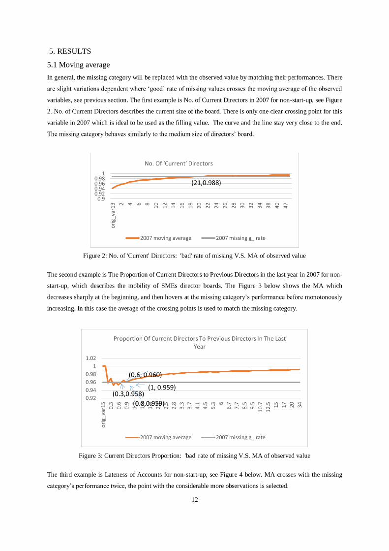
variables, see previous section. The first example is No. of Current Directors in 2007 for non-start-up, see Figure

2. No. of Current Directors describes the current size of the board. There is only one clear crossing point for this

variable in 2007 which is ideal to be used as the filling value. The curve and the line stay very close to the end.

The missing category behaves similarly to the medium size of directors’ board.

Figure 2: No. of 'Current' Directors: 'bad' rate of missing V.S. MA of observed value

The second example is The Proportion of Current Directors to Previous Directors in the last year in 2007 for non-

start-up, which describes the mobility of SMEs director boards. The Figure 3 below shows the MA which

decreases sharply at the beginning, and then hovers at the missing category’s performance before monotonously

increasing. In this case the average of the crossing points is used to match the missing category.

Figure 3: Current Directors Proportion: 'bad' rate of missing V.S. MA of observed value

The third example is Lateness of Accounts for non-start-up, see Figure 4 below. MA crosses with the missing

category’s performance twice, the point with the considerable more observations is selected.

0.90.920.940.960.98

1

ori

g_va

r13 2 4 6 8 10

12

14 16 18

20

22

24

26

28 30 32

34

38

40

47

No. Of ‘Current’ Directors

2007 moving average 2007 missing g_ rate

(21,0.988)

0.92

0.94

0.96

0.98

1

1.02

ori

g_va

r15

0.3

0.6

0.9

1.2

1.5

1.8

2.2

2.5

2.8

3.3

3.7

4.1

4.5

5.3 6

6.7

7.7

8.5

9.5

10.7

12.5 15 17

20

34

Proportion Of Current Directors To Previous Directors In The Last Year


(1, 0.959)

(0.8,0.959)

(0.6, 0.960)

(0.3,0.958)

13

Figure 4: Lateness of Account: 'bad' rate of missing V.S. MA of observed value

The fourth example is Proportion of Current Directors to Previous Directors in the Last Year for start-up, see

Figure 5. Although there is no real crossing point, the point where the line and the MA curve are the smallest

distance apart is chosen to approximate the performance of missing category.

Figure 5: Proportion of Current Directors: 'bad' rate of missing V.S. MA of observed value

The fifth example is Total Assets for start-up, see Figure 6. Its original value covers a very large range with

79.33% missing rate. Owing to the volatility of the moving average and the size of missing category, WoE is used

for Total Assets in order to avoid more noise.

0

0.2

0.4

0.6

0.8

1

1.2

ori

g_va

r49 -6 14

34

54

74

94

11

4

13

4

15

4

17

4

19

4

21

4

23

4

25

4

27

4

29

4

31

4

33

6

36

0

38

2

40

9

45

0

48

8

53

2

58

8

66

0

75

6

89

0

Lateness Of Accounts


(1.2, -22.5)

(261, 0.987)

0.85

0.9

0.95

1

1.05

ori

g_va

r15

0.2

0.4

0.6

0.8

1.3

1.7 2

2.5

2.7

3.3

3.7

4.5

5.3 6

6.5 7 8

10

12

14

16

20

28

.7

Proportion Of Current Directors To Previous Directors In The Last Year

myflagA missrate

14

Figure 6: Total Assets: 'bad' rate of missing V.S. MA of observed value

Finally, because massive amount of missing values is found on Time since Last Derogatory Data Item (Months)

for both Non-Start-ups and Start-ups, we can compare the performance. For Start-ups (Figure 7), MA increases

almost monotonously, while the missing category shows a distinct performance and is always above the MA curve.

Since the crossing point would be perceived as an outlier then the maximum value is used as approximation to

impute the missing value. For Non-Start-ups (Figure 8), there is only one crossing point whose derogatory data

is recorded long ago. Given the difference, it is reasonable to treat Start-ups and Non-Start-ups SMEs separately.

Figure 7: Time since Last Derog. Data: 'good' rate of missing V.S. MA of observed value of Start-ups

00.10.20.30.40.50.60.70.80.9

1

ori

g_va

r46 0 1 2 3 4 5 6 7 8 9 10 11 12 13 14 15 16 17 18 19 20 21 23 24 26

Time since last derogatory data item (months)


(40, 0.925)

15

Figure 8: Time since Last Derog. Data: 'bad' rate of missing V.S. MA of observed value of Non-Start-ups

In summary, the missing category’s performance of start-up SMEs could not be easily replaced by observed values

and the missing category’s performance is less stable compared to ‘Non-Start-ups.’ Approximation is used when

no exact crossing exists. However, as more approximations are used in this segment, there is a potential loss of

information, which could cause reduction in the predicted accuracy when using variables in their original format.

5.2 Multiple imputation by chained equations

The whole sample is subdivided into Start-ups and Non-Start-ups, and the variables used in imputation process

has been determined based on (Ma, 2017). Likewise, continuous variables (nominal variables), binary variables

and categorical variables are imputed by PMM, logistic regression, and multinomial logistic regression

respectively. Some researchers suggested to impute on the raw scale with no restrictions to the range, and with no

post-imputation rounding. Although this imputation method results in some implausible values, it appears to be

the most consistent method with low bias and reliable coverage in repeated sampling of missingness, irrespective

of the amount of skewness in the data (von Hippel, 2013; Rodwell et al., 2014). The imputation procedure

produces up to 100 imputed datasets with 50 maximum iterations for empirical variables with a fixed seed as well.

Finally, Logistic regression is also used to pool estimates by Rubin’s rules. The pooled estimates of selected

variables of Start-ups and Non-Start-ups are presented in

0

0.2

0.4

0.6

0.8

1

1.2

ori

g_va

r44 8 17

26

35 44 53

62

71

80 89 98

107

11

61

25

13

41

43

152

16

11

70

17

91

88

19

72

06

215

22

42

33

24

22

51

260

27

13

10

35

14

00

Time since last derogatory data item (months)


(228, 0.963)

16

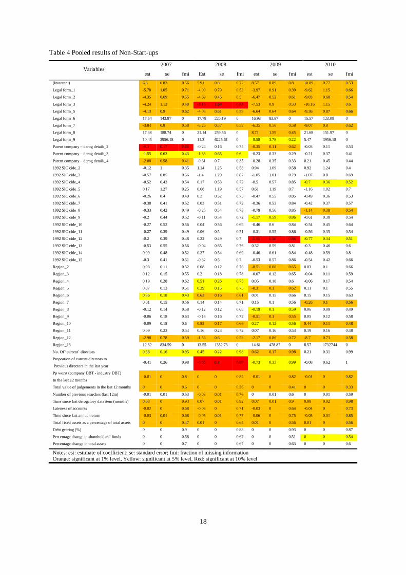
Table 3 and Table 4, respectively. As mention early, the column FMI is the proportion of the total variance that

is owing to the missing data (FMI = (VB+ VB /m)/VT).

As expected, the majority of variables are statistically significant. Yet, the contribution of 1992 SIC code is not

during the completely observed periods for both segments, which is consistent to previous conclusions. Regions

seems not to be a significant predictor for Non-Start-ups. However, there are unexpected findings. The high

missing rate should come with high FMI. The pooled standard error should be higher than that from single imputed

dataset because of between-imputation variance (VB) and the extra variation due to the number of imputation

(VB/m). Variables: Proportion Of Current Directors To Previous Directors In The Last Year, Time since last

derogatory data item (months), Time Since Last Annual Return, and Total Assets in Start-ups, and Proportion Of

Current Directors To Previous Directors In The Last Year, PP Worst (Company DBT - Industry DBT) In The Last

12 Months, Time since last derogatory data item (months), and Debt Gearing (%) in Non-Start-ups have extremely

low standard error and coefficient estimates, given an extremely high FMI and missing rate over 50%.

17

Table 3 Pooled results of Start-ups

Variables 2007 2008 2009 2010

est se fmi Est se fmi est se fmi est se fmi

(Intercept) 3.58 0.86 0.5 1.19 0.44 0.62 1.43 0.37 0.54 1.1 0.59 0.74

Legal form_1 -2.94 0.78 0.29 -2.23 0.65 0.62 -2.56 0.46 0.25 -2.91 0.85 0.55

Legal form_2 -3.64 0.52 0.18 -2.38 0.21 0.52 -2.41 0.15 0.3 -3.17 0.19 0.23

Legal form_3 -3.73 0.9 0.47 -2.16 0.63 0.53 -1.23 0.56 0.16 -2.23 0.59 0.2

Legal form_5 -2.59 0.69 0.38 -0.88 0.38 0.46 -0.72 0.31 0.44 -2.7 0.31 0.36

Legal form_6 9.68 93.58 0 12.02 98.47 0 11.82 94.9 0 11.38 90.42 0

Legal form_7 -2.73 0.63 0.35 -1.28 0.33 0.58 -1.28 0.22 0.35 -2.59 0.25 0.32

Legal form_8 11.07 320.55 0 13.35 393.8 0 13.7 461.22 0 12.45 534.15 0

Legal form_9 10.78 1455.4 0

Company is subsidiary_2 -0.25 0.24 0.71 1.11 0.2 0.7 1.69 0.12 0.32 1.18 0.17 0.45

Company is subsidiary_4 -0.35 0.74 0.9 0.18 0.58 0.59 2.63 0.53 0.19 1.25 0.54 0.45

1992 SIC code_2 2.08 112.18 0 -0.1 0.9 0.53 0.41 1.01 0.44 0.36 1.13 0.69

1992 SIC code_3 -0.55 1.08 0.77 -0.06 0.64 0.58 0.26 0.67 0.62 -0.79 0.8 0.7

1992 SIC code_4 -0.42 0.72 0.71 -0.59 0.39 0.63 0.11 0.32 0.53 0.08 0.57 0.8

1992 SIC code_5 -0.09 1.2 0.58 -0.62 0.81 0.65 0.45 0.66 0.56 0.24 0.78 0.72

1992 SIC code_6 -0.22 0.68 0.69 -0.37 0.36 0.62 0.24 0.3 0.52 0.08 0.55 0.81

1992 SIC code_7 -0.52 0.7 0.71 -0.2 0.36 0.63 0.04 0.3 0.53 0.04 0.55 0.8

1992 SIC code_8 -0.45 0.71 0.7 -0.38 0.39 0.65 0.12 0.31 0.52 0.07 0.57 0.8

1992 SIC code_9 -0.35 0.72 0.72 -0.29 0.37 0.61 -0.02 0.31 0.52 0.14 0.58 0.8

1992 SIC code_10 -0.36 0.79 0.74 -0.53 0.41 0.63 0.09 0.35 0.57 0.2 0.63 0.81

1992 SIC code_11 -0.37 0.69 0.71 -0.26 0.34 0.59 0.1 0.3 0.54 0.2 0.56 0.82

1992 SIC code_12 -0.43 0.7 0.72 -0.29 0.34 0.59 -0.01 0.3 0.55 0.11 0.55 0.81

1992 SIC code_13 -0.39 0.77 0.72 -0.18 0.44 0.64 0.14 0.36 0.53 0.26 0.61 0.8

1992 SIC code_14 -0.73 0.74 0.72 -0.52 0.4 0.65 0.09 0.32 0.54 0.26 0.56 0.79

1992 SIC code_15 -0.41 0.71 0.72 -0.22 0.36 0.62 0.1 0.3 0.53 0.17 0.56 0.81

Region_2 0.12 0.09 0.66 -0.12 0.07 0.53 0.22 0.06 0.29 0.24 0.07 0.5

Region_3 0.24 0.13 0.52 0.26 0.11 0.56 0.25 0.08 0.34 0.26 0.1 0.41

Region_4 0.09 0.21 0.52 0.32 0.19 0.52 0.18 0.13 0.28 0.13 0.17 0.5

Region_5 0.18 0.1 0.61 -0.48 0.08 0.62 0.12 0.06 0.27 0.12 0.08 0.41

Region_6 0.51 0.17 0.56 0.29 0.15 0.64 0.14 0.09 0.3 0.26 0.13 0.51

Region_7 0.25 0.1 0.48 0.18 0.1 0.6 0.34 0.07 0.33 0.1 0.08 0.4

Region_8 0.21 0.12 0.67 0.04 0.1 0.67 0.26 0.06 0.32 0.24 0.08 0.48

Region_9 -0.05 0.13 0.65 -0.18 0.1 0.54 0.24 0.08 0.33 0.06 0.09 0.45

Region_10 0.5 0.14 0.47 0.99 0.12 0.4 0.38 0.1 0.39 0.37 0.1 0.4

Region_11 0.39 0.21 0.6 -0.04 0.18 0.64 0.21 0.12 0.23 -0.2 0.15 0.48

Region_12 -1.25 0.81 0.52 -2.14 0.52 0.66 0.33 0.35 0.37 -1.41 0.34 0.64

Region_13 8.24 515.22 0 12.46 428.03 0 -0.59 1.41 0.12 475.06 0


previous directors in the last year 0.27 0.1 0.92 0.14 0.09 0.94 -0.41 0.08 0.91 0.18 0.08 0.91

Oldest age of current directors

/proprietors supplied (years) 0.01 0 0.73 0.01 0 0.72 0.02 0 0.46 0.01 0 0.53

Number of directors holding shares 0.11 0.06 0.72 0.93 0.05 0.66 1.14 0.04 0.48 0.78 0.04 0.53

Total value of judgements in the last 12 months 0 0 0.39 0 0 0.43 0 0 0.06 0 0 0.11

Number of previous searches (last 12m) -0.03 0.02 0.74 0.01 0.02 0.69 0.05 0.01 0.35 0.08 0.01 0.4

Time since last derogatory data item (months) 0.42 0.03 0.88 0.39 0.03 0.93 0.37 0.03 0.91 0.42 0.03 0.89

Lateness of accounts -0.15 0.01 0.71 -0.17 0 0.68 -0.18 0 0.5 -0.18 0 0.54

Time since last annual return -0.15 0.01 0.77 -0.14 0.01 0.6 -0.15 0 0.45 -0.13 0.01 0.64

Total assets 0 0 0.91 0 0 0.9 0 0 0.84 0 0 0.79

Notes: est: estimate of coefficient; se: standard error; fmi: fraction of missing information

Orange: significant at 1% level, Yellow: significant at 5% level, Red: significant at 10% level

18

Table 4 Pooled results of Non-Start-ups

Variables 2007 2008 2009 2010

est se fmi Est se fmi est se fmi est se fmi

(Intercept) 6.6 0.83 0.56 5.91 0.8 0.72 8.57 0.89 0.8 10.89 0.77 0.53

Legal form_1 -5.78 1.05 0.71 -4.09 0.79 0.53 -3.97 0.91 0.39 -9.62 1.15 0.66

Legal form_2 -4.35 0.69 0.55 -4.69 0.45 0.5 -6.47 0.52 0.61 -9.03 0.68 0.54

Legal form_3 -4.24 1.12 0.48 -3.16 1.64 0.63 -7.53 0.9 0.53 -10.16 1.15 0.6

Legal form_5 -4.13 0.9 0.62 -4.03 0.61 0.59 -6.64 0.64 0.64 -9.36 0.87 0.66

Legal form_6 17.54 143.87 0 17.78 220.19 0 16.93 83.87 0 15.57 123.08 0

Legal form_7 -3.84 0.8 0.58 -5.26 0.57 0.58 -6.35 0.56 0.58 -9.07 0.8 0.62

Legal form_8 17.48 188.74 0 21.14 259.56 0 8.71 1.59 0.45 21.68 151.97 0

Legal form_9 10.45 3956.18 0 11.3 6225.61 0 -8.58 3.78 0.22 5.47 3956.18 0

Parent company – derog details_2 -0.3 0.17 0.66 -0.24 0.16 0.75 -0.35 0.11 0.62 -0.03 0.11 0.53

Parent company – derog details_3 -1.55 0.63 0.43 -1.33 0.65 0.6 -0.23 0.33 0.29 -0.21 0.37 0.41

Parent company – derog details_4 -2.08 0.58 0.41 -0.61 0.7 0.35 -0.28 0.35 0.33 0.21 0.45 0.44

1992 SIC cide_2 -0.12 1 0.35 1.14 1.25 0.58 0.94 1.09 0.58 0.92 1.24 0.4

1992 SIC cide_3 -0.57 0.85 0.56 -1.4 1.29 0.87 -1.05 1.01 0.79 -1.07 0.8 0.69

1992 SIC cide_4 -0.52 0.43 0.54 0.17 0.53 0.72 -0.5 0.57 0.85 -0.7 0.36 0.52

1992 SIC cide_5 0.17 1.27 0.25 0.68 1.19 0.57 0.61 1.19 0.7 -1.16 1.02 0.7

1992 SIC cide_6 -0.26 0.4 0.49 0.2 0.52 0.73 -0.47 0.55 0.85 -0.49 0.36 0.53

1992 SIC cide_7 -0.38 0.41 0.52 0.03 0.51 0.72 -0.36 0.53 0.84 -0.42 0.37 0.57

1992 SIC cide_8 -0.33 0.42 0.49 -0.25 0.54 0.73 -0.79 0.56 0.85 -1.14 0.38 0.54

1992 SIC cide_9 -0.2 0.44 0.52 -0.11 0.54 0.72 -1.17 0.59 0.86 -0.61 0.38 0.54

1992 SIC cide_10 -0.27 0.52 0.56 0.04 0.56 0.69 -0.46 0.6 0.84 -0.54 0.45 0.64

1992 SIC cide_11 -0.27 0.39 0.49 0.06 0.5 0.71 -0.31 0.55 0.86 -0.56 0.35 0.54

1992 SIC cide_12 -0.2 0.39 0.48 0.22 0.49 0.7 -1.05 0.56 0.86 -0.77 0.34 0.51

1992 SIC cide_13 -0.53 0.55 0.56 -0.04 0.65 0.76 0.32 0.59 0.81 -0.3 0.46 0.6

1992 SIC cide_14 0.09 0.48 0.52 0.27 0.54 0.69 -0.46 0.61 0.84 -0.48 0.59 0.8

1992 SIC cide_15 -0.3 0.41 0.51 -0.32 0.5 0.7 -0.53 0.57 0.86 -0.54 0.42 0.66

Region_2 0.08 0.11 0.52 0.08 0.12 0.76 -0.51 0.08 0.65 0.03 0.1 0.66

Region_3 0.12 0.15 0.55 0.2 0.18 0.78 -0.07 0.12 0.65 -0.04 0.11 0.59

Region_4 0.19 0.28 0.62 0.51 0.26 0.75 0.05 0.18 0.6 -0.06 0.17 0.54

Region_5 0.07 0.13 0.51 0.29 0.15 0.75 -0.3 0.1 0.62 0.11 0.1 0.55

Region_6 0.36 0.18 0.43 0.63 0.16 0.61 0.01 0.15 0.66 0.15 0.15 0.63

Region_7 0.01 0.15 0.56 0.14 0.14 0.71 0.15 0.1 0.56 -0.26 0.1 0.56

Region_8 -0.12 0.14 0.58 -0.12 0.12 0.68 -0.19 0.1 0.59 0.06 0.09 0.49

Region_9 -0.06 0.18 0.63 -0.18 0.16 0.72 -0.51 0.1 0.55 0.05 0.12 0.58

Region_10 -0.09 0.18 0.6 0.83 0.17 0.66 0.27 0.12 0.56 0.44 0.11 0.48

Region_11 0.09 0.23 0.54 0.16 0.23 0.72 0.07 0.16 0.53 0.19 0.16 0.48

Region_12 -2.98 0.78 0.59 -1.56 0.6 0.58 -2.17 0.86 0.72 -8.7 0.73 0.58

Region_13 12.32 834.59 0 13.55 1352.73 0 14.61 478.87 0 8.57 1732744 0

No. Of ‘current’ directors 0.38 0.16 0.95 0.45 0.22 0.98 0.62 0.17 0.98 0.21 0.31 0.99


Previous directors in the last year -0.41 0.26 0.98 -0.65 0.4 0.99 -0.73 0.33 0.99 -0.08 0.62 1

Pp worst (company DBT - industry DBT)

In the last 12 months -0.01 0 0.8 0 0 0.82 -0.01 0 0.82 -0.01 0 0.82

Total value of judgements in the last 12 months 0 0 0.6 0 0 0.36 0 0 0.41 0 0 0.33

Number of previous searches (last 12m) -0.01 0.01 0.53 -0.03 0.01 0.76 0 0.01 0.6 0 0.01 0.59

Time since last derogatory data item (months) 0.03 0 0.93 0.07 0.01 0.92 0.07 0.01 0.9 0.08 0.02 0.98

Lateness of accounts -0.02 0 0.68 -0.03 0 0.71 -0.03 0 0.64 -0.04 0 0.73

Time since last annual return -0.03 0.01 0.68 -0.05 0.01 0.77 -0.06 0 0.75 -0.05 0.01 0.85

Total fixed assets as a percentage of total assets 0 0 0.47 0.01 0 0.65 0.01 0 0.56 0.01 0 0.56

Debt gearing (%) 0 0 0.9 0 0 0.88 0 0 0.93 0 0 0.87

Percentage change in shareholders’ funds 0 0 0.58 0 0 0.62 0 0 0.51 0 0 0.54

Percentage change in total assets 0 0 0.7 0 0 0.67 0 0 0.63 0 0 0.6

Notes: est: estimate of coefficient; se: standard error; fmi: fraction of missing information

Orange: significant at 1% level, Yellow: significant at 5% level, Red: significant at 10% level

19

Figure 9 and Figure 10 provides convergence plots (the left one is mean, and the right one is standard deviation)

for both Start-ups and Non-Start-ups SMEs. In this section, the convergence plots of variables with over 50%

missing rate are presented and discussed.

2007

2008

20

09

20

10

Notes: ref03_03: Proportion of current directors to previous directors in the last year; ref07_38: Time since last derogatory data item

(months); ref10_13: Time since last annual return; ref10_19: Total assets

Figure 9 Convergence plots of variables over 50% missing rate for Start-ups

Convergence results seem to be better as an increase of numbers of iteration and numbers of imputation. In 2009,

the proportion of current directors to previous directors in the last year and time since last derogatory data item

(months) in Figure 9 see an initial trend going upwards and downwards, respectively, and the trend remains till

the end of the iteration.

20

2007

2008

2009

20

10

Notes: ref03_03: Proportion of current directors to previous directors in the last year; ref04_05: Pp worst (company DBT - industry DBT)

in the last 12 months; ref07_38: Time since last derogatory data item (months); ref10_48: Debt gearing (%)

Figure 10 Convergence plots of variables over 50% missing rate for Non-Start-ups

In terms of Non-Start-ups variables (Figure 10), an initial trend can be found on variables proportion of current

directors to previous directors in the last year and time since last derogatory data item (months), but the trend

eventually remains stable. One of the worst convergences is proportion of current directors to previous directors

in the last year in 2010. The plot shows a binary path. One path keeps stable since imputation begins, and another

one remains static after an initial rising trend. Both paths do not converge until the end. These problematic

variables have an extremely high FMI, and it would be appropriate to increase the numbers of iteration or to

require more correlated variables into the imputation process to obtain a more stable imputation results.

Figure 11 provides a series of density plots of missing variables from 2007 to 2010 for both Start-ups and Non-

Start-ups SMEs. As shown in the missing rate table, variables have missing values ranging from less than 1% to

up to 96.7%. On the left panel, imputed Lateness of accounts shows a “bell” shape, while the observed values are

not. Due to less than 1% missing number, extreme values affect the shape of the plots dramatically. A similar

situation can be found on the variable Number of directors holding shares. Another important variable needed to

be checked is Time since last derogatory data item (months) because of its large missing rate. Intuitively, once

this variable is greater than ten on the x-axis, observed and imputed values roughly overlap. Imputed values are

approximately greater than the observed in the range of zero to ten. Imputed values are higher since short time

since last derogatory data item is unwilling to report. Besides, impute values of other variables seem to have a

good fit of the observed values.

21

Start-ups Non-Start-ups 2007

2008

20

09

20

10

Notes: The “blue” curve is generated by the observed value and the “red” curve by imputed values from various imputed dataset. ref03_01:

No. Of ‘current’ directors; ref03_03: Proportion of current directors to previous directors in the last year; ref03_08: Oldes t age of current

directors/proprietors supplied (years); ref03_09: Number of directors holding shares; ref04_05: Pp worst (company DBT - industry DBT)

in the last 12 months; ref05_04: Total value of judgements in the last 12 months; ref06_03: Number of previous searches (last 12m);

ref07_38: Time since last derogatory data item (months); ref10_01: Lateness of accounts; ref10_13: Time since last annual return;

ref10_19: Total assets; ref10_30: Total fixed assets as a percentage of total assets; ref10_48: Debt gearing (%); ref11_01: P ercentage

change in shareholders’ funds; ref11_04: Percentage change in total assets.

Figure 11 Density plot of continuous variables

On the right panel in Figure 11, imputation results seem to be much more problematic than that of Start-ups.

Missing rates of these variables: Proportion of current directors to previous directors in the last year, PP worst

(company DBT - industry DBT) in the last 12 months, time since the last derogatory data item (months), and Debt

gearing (%), are over 50%, and the others are less than 9%. There is a good fit between observed and imputed

values of PP worst (company DBT - industry DBT) in the last 12 months and Debt gearing (%). The gap between

observed and imputed values of Proportion of current directors to previous directors in the last year is found on

the lower x-axis. As the proportion increases, the gap gradually disappears. It is different from Start-ups of time

since the last derogatory data item (months). Imputed values are smaller than observed values at a lower range of

x-axis due to the beginning of the financial crisis.

22

5.3 GAMs results

A final GAM model was established based on the response variable and its significant influential predictors using

the imputed dataset. For comparison purpose, the data has been standardlized, and the GAM results are generated

by SAS and R (mgcv package). The specific importance and effect of each predictor imposed on the response can

be examined from the GAM results. Contributions for predictor variables in the GAM, and the effect of each

predictor can be partitioned and examined by the smooth function plots. The plot presents varying magnitude of

the effect of each variable where the y-axis represents the contribution (effect) of each covariate to the fitting

response, centred on zero. The numbers in the labels of the y-axis denote the effective degrees of freedom. The

relative density of data points is shown by the rug plot on the x-axis. Rug plots are particularly useful in connection

with additive models where the plotted smooth function is used to assess how much data contributed to the model

fit at the different values of the independent variables. Estimated smooth functions (solid lines) with 95%

confidence intervals (shaded area) are shown for each predictor. The positive slope of smoothed line indicates

positive effect of the predictor imposed on the ‘good’ estimation, and vice versa. The narrow confidence limits

indicate high relevance and wide confidence limits indicated low relevance ranges of distribution (Solanki et al.,

2017). In the following, some variables will be presented for illustration and discussion.

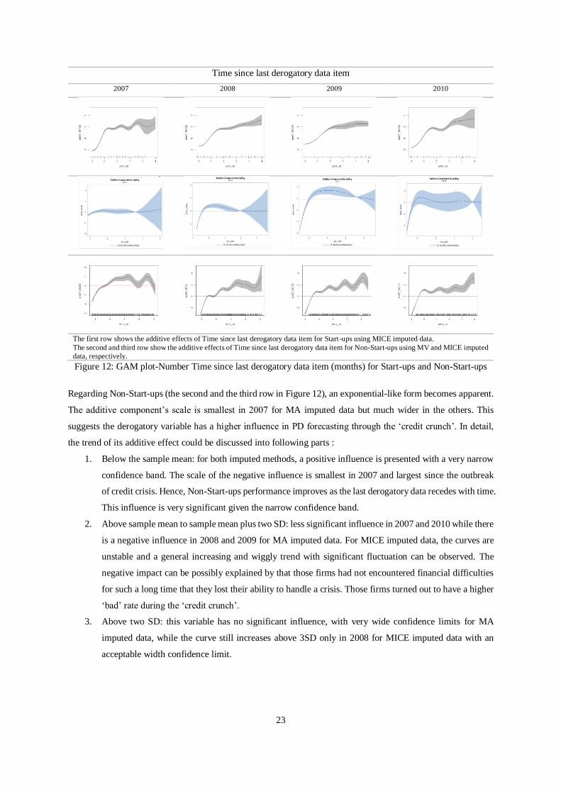
5.3.1 Time since last derogatory data item

Time since last derogatory data item has the largest proportion of missing data in the dataset. A derogatory item

is negative and typically indicates serious delinquency or late payments. Derogatory items represent credit risk to

lenders, and therefore, are likely to have a substantial effect on the ability to obtain new credit for borrowers. The

firm’s derogatory data is collected from various public sources for a more complete record of the firm’s previous

history. Public record items, such as bankruptcies, tax, and judgments also are considered derogatory. While some

lenders still may be willing to extend credit to someone with derogatory items on their report, they may do so with

higher interest rates or fees. Therefore, it is intuitively expected that the shorter time since the last derogatory, the

worst the credit quality is.

Regarding Start-ups, as mentioned above in MA methods, the approximately maximum values are used to impute

the missing values, and this is not well replicated for Start-ups SMEs. Therefore, its performance does not discuss

here. On the other hand, under the MICE-imputed data, the smooth function plot (the first row in Figure 12) can

be divided into two parts for discussion:

1. Below sample mean: An initially flat curve is found in 2008, but an overall positive influence is presented

from 2007 to 2010 in general.This impact is very significant because of a very narrow confidence band.

The curve in 2007 is steeper than others.

2. Above sanple mean: in general, the curve is still climbing but with fluctuations in 2007 and 2010, though,

at a lower rate. Two peaks are observed in 2007, while other curves are relatively flat. This variable has

less significant influence in 2010 due to large confidence limits, and its curve is relatively flat. Other

curves still show a rising trend with reasonable confidence bands.

23

Time since last derogatory data item

2007 2008 2009 2010

The first row shows the additive effects of Time since last derogatory data item for Start-ups using MICE imputed data.

The second and third row show the additive effects of Time since last derogatory data item for Non-Start-ups using MV and MICE imputed

data, respectively.

Figure 12: GAM plot-Number Time since last derogatory data item (months) for Start-ups and Non-Start-ups

Regarding Non-Start-ups (the second and the third row in Figure 12), an exponential-like form becomes apparent.

The additive component’s scale is smallest in 2007 for MA imputed data but much wider in the others. This

suggests the derogatory variable has a higher influence in PD forecasting through the ‘credit crunch’. In detail,

the trend of its additive effect could be discussed into following parts :

1. Below the sample mean: for both imputed methods, a positive influence is presented with a very narrow

confidence band. The scale of the negative influence is smallest in 2007 and largest since the outbreak

of credit crisis. Hence, Non-Start-ups performance improves as the last derogatory data recedes with time.

This influence is very significant given the narrow confidence band.

2. Above sample mean to sample mean plus two SD: less significant influence in 2007 and 2010 while there

is a negative influence in 2008 and 2009 for MA imputed data. For MICE imputed data, the curves are

unstable and a general increasing and wiggly trend with significant fluctuation can be observed. The

negative impact can be possibly explained by that those firms had not encountered financial difficulties

for such a long time that they lost their ability to handle a crisis. Those firms turned out to have a higher

‘bad’ rate during the ‘credit crunch’.

3. Above two SD: this variable has no significant influence, with very wide confidence limits for MA

imputed data, while the curve still increases above 3SD only in 2008 for MICE imputed data with an

acceptable width confidence limit.

24

Trend consistency for all four years Trend of additive effects Interval with narrow confidence band

MICE_Start-ups Almost constant Exponential-like (-SD, SD)

MA_Non-Start-ups Almost constant Exponential-like Below sample mean

MICE_Non-Start-ups Switch sign at 2.5SD in 2008 Exponential-like Below sample mean

Figure 13: Summary of additive effects of Time since last derogatory data item (months)

The derogatory data is especially important if the record is more recent for both Start-ups and Non-Start-ups .

SMEs with a recent derogatory record significantly jeopardize SMEs’ performance, but this effect gradually

weaken with time.

5.3.2 Lateness of accounts

For the retail consumers, their detailed account information could be updated by daily transition.

Other information such as change of address is usually modified to the bank on time as well.

The liquidity of corporation’s stock leads to the frequent adjustment for their assets market

price. The discrete time feature of SMEs accounting information challenges the application of

various types of credit models.

Lateness of accounts

2007 2008 2009 2010

The first and second row show the additive effects of Lateness of accounts for Start-ups using MV and MICE imputed data respectively.

25

The third and fourth row show the additive effects of Lateness of accounts for Non-Start-ups using MV and MICE imputed data,

respectively.

Figure 14: GAM plot- Lateness of accounts for Start-ups and Non-Start-ups

Regarding Start-ups for MV imputed data (the first row in Figure 14), the additive effect has a clear quadratic

form in 2007, a polynomial-like form with a degree of three in 2008 and 2010 and a clear polynomial form with

a degree of three in 2009. Hence, the pattern of this variable can be divided into three parts:

1. Below the sample mean, this variable presents a positive influence with a wider confidence band. Hence,

if Start-ups’ account update duration is shorter than the sample mean, the longer the duration since the

last account update, the better performance it will have. It means that if the firm can survive with a longer

Lateness of Accounts, its surviving ability increases as well. However, this prediction comes with higher

uncertainty, suggested by the wide confidence band.

2. From sample mean to mean plus two SD, negative influence with narrow confidence band. Hence,

Lateness of Accounts is most predictive for Start-ups that fall into this part. Start-ups’ performance

decreases as the time since the last accounting update becomes longer.

3. Above mean plus two SD: switched influence through time. This part is shorter, with a negative

coefficient and wide confidence band in 2007. It stays flat in 2008 and 2010. However, a clear positive

effect is perceived with a narrow confidence band in 2009, which is capturted by MICE imputed data at

around 2SD as well. It is the most obvious sign of switching for start-ups during the financial crisis. Start-

ups that survived through the ‘credit crunch’ gain ‘swimming’ ability to increase performance.

However, MICE imputed data shows different results (the second row in Figure 14). The variable presents a

linearly negative influence with a wide confidence band at each tail of all years. A narrow confidence limit is

observed from -SD to 2 SD. The longer the duration since the last account update, the worst performance Start-

ups will have. Considering the stable shape of the overall trend, it can conclude that the business cycle would not

affect this variable significantly, which is a contradiction of MA imputed data.

Regarding MA imputed data for Non-Start-ups, this variable presents a quadratic form for the additive effect, and

the changing point is always around the sample mean. Therefore, the impact of Lateness of Accounts can be

separated into two parts:

1. Below the sample mean: SMEs’ performance decreases as their Lateness of Accounts increase. This part

has a negative influence with a very narrow confidence band. Hence, as the SMEs’ accounts becomes

more dated, they tend to exhibit a worse performance. This trend is consistent regardless the business

cycle.

2. Above the sample mean: Lateness of Accounts has a positive influence with a wider and wider confidence

band. This means those ‘Non-Start-ups’ becomes less predictable due to the changing economy.

Regarding MICE imputed data for Non-Start-ups, this variable presents a polynomial form for the additive effect,.

Therefore, the impact of Lateness of Accounts can be separated into following parts:

26

1. Below sample mean: the curve presents an increasing trend in 2007 and 2008 while an inverse trend in

2009 and 2010. The changes in the economic environment have a great impact on this variable due to

the different shape of plots.

2. From sample mean to SD: all curves have a narrow confidence band with negative slope.

3. Above SD: this part shows a quadratic form with wider confidence band.

In summary, Lateness of Accounts is most informative for Start-ups and Non-Start-ups when it falls between the

sample mean to mean plus one SD, showing a negative influence with narrow confidence band. Below this interval,

this variable’s prediction has a higher degree of uncertainty, indicated by the wide confidence band. Above this

interval, the ‘Start-ups’’ performance varies over time. The newer the account information is, the better

performance the firm will have. For firms that update their account over a longer period than the sample mean,

their performance is influenced by the ‘credit crunch’ and becomes less predictable.


MA_Start-ups Almost constant Quadratic or polynomial-like (Mean,SD)

MICE_Start-ups Almost constant Polynomial-like (-SD,2SD)

MA_Non-Start-ups Almost constant L' shape-like Below sample mean

MICE_Non-Start-ups Quite different Polynomial-like (-0.5SD,SD)

Figure 15: Summary of additive effects of Lateness of accounts

5.3.3 Time since last annual return

According to the UK government, companies are required to send their annual return one year after either

incorporation of the company or date you filed your last annual return. It should be completed up to 28 days after

the due date. It mainly contains firms’ general information rather than accounting ratios describing the functioning

of the firm (GOVUK, 10 Dec., 2014):

• officers’ information----firm directors and secretaries general;

• SIC----classification of firm’s business type;

• Capital snapshot which is required for firms that have share capital.

Time since Last Annual Return tells the duration since a firm last reported its general information. It helps

supervisors and banks to gather more information about this firm for the purpose of ‘communication, influence,

training and support, investigation and others’ (Annual Return 2010, Standards for England). Keasey and Watson

(1986) has used a similar variable, lags in reporting to the Companies House, to model UK SMEs’ defaults. It

provides a snapshot of the firm and is used to guarantee sufficient information is provided to Companies House.

Hence, being able to provide its annual return indicates that the firm is being run under normal circumstances by

the known directors with a clearly stated amount of capital.

Regarding Start-ups for MV and MICE imputed data (the first and second row in Figure 16), the variable’s

additive effect shows an almost linear pattern. A clear negative coefficient is perceived, with a narrow confidence

band. As mentioned previously, Time since Last Annual Return marks the duration since the last time the firm

reported to Companies House. The longer the time since last reporting, the opaquer the firm’s information. This

27

is a very strong conclusion. It tells banks that even if they cannot collect detailed ‘soft’ information on SMEs,

banks can still separate ‘good’ SMEs from ‘bad’ according to the punctuality of their annual returns. This

influence is especially strong during the ‘credit crunch’, which is 2008 and 2009.

2007 2008 2009 2010

The first and second row show the additive effects of Time since Last Annual Return for Start-ups using MV and MICE imputed data

respectively.

The third and fourth row show the additive effects Time since Last Annual Return for Non-Start-ups using MV and MICE imputed data,

respectively. Figure 16: GAM plot-Time since Last Annual Return for Start-ups and Non-Start-ups

Regarding Non-Start-ups, a quadratic form is seen in 2007 and 2008, and then a higher order polynomial of degree

three in 2009 and 2010, see Figure 16. Hence, the additive effect can be divided into following parts:

1. A rapid decrease with a narrow confidence band. This is observed below the sample mean for MA

imputed data and below one SD for MICE data. The longer duration since their last annual return is

correlated with worse performance. The influence of this part stays constant through the financial crisis.

2. Tthe influence of thevariable becomes positive from sample mean to sample mean plus one SD for for

MA imputed data and from one SD to three SD for MICE data. In this part, with wider confidence limits.

It indicates that firms falling into this part gain survival ability through time. The longer the duration

since their last annual return, the more knowledge they gain to keep their business from financial

constraints.

28

3. For MA imputed data above sample mean plus one SD, the annual return has an almost constant effect,

with widest confidence limits especially before and after the financial crisis. The firms have not reported

to the Company House for a long time. These firms’ information becomes opaque and their performance

is therefore difficult to predict given the information. However, for MIC imputed data above three SD,

an inverse trend is observed again since the outbreak of credit crisis.


MA_Start-ups Almost constant Quadratic or polynomial-like (-SD,2SD)

MICE_Start-ups Almost constant Quadratic or polynomial-like (-SD,2SD)

MA_Non-Start-ups Almost constant Quadratic or polynomial-like Below sample mean

MICE_Non-Start-ups Switch trend above 3SD in 2007 Quadratic or polynomial-like Below sample mean

Figure 17: Summary of additive effects of Time since last annual return

In summary, this part presents independent variables trend for ‘start-up’ SMEs. There are fewer continuous

variables analysed in their original format for ‘Start-ups’ due to the distinct performance of missing categories.

However, the trend of their additive effects is not more volatile than that of ‘Non-Start-ups’. For example, Time

since Last Annual Return presents an almost constant decrease pattern. Compared to ‘Non-Start-ups’, the tail

performance is less volatile since the ‘Start-ups’’ records are much more recent. Time since last annual return

marks the duration since the last time the firm reported to Companies House. The shorter the time since the last

reporting, the more transparent the SME’s information. This is a very strong conclusion, which can help banks

separate ‘good’ SMEs from ‘bad’ according to the punctuality of their annual return even if SMEs do not provide

detailed ‘soft’ information.

The scale of additive effects is very large over all four years, with a very narrow confidence band below the sample

mean. Although one cannot gather more detailed information about the firms without further investigation, this

research shows that Time since Last Annual Return is a key variable in judging SMEs’ performance. ‘Non-Start-

ups’ should regularly release their information to the public. This variable has a similar trend to Lateness of

Accounts, as both variables describe the frequency with which a company updates its information. The two

variables are not highly correlated since they are collected from different sources. Lateness of Accounts is usually

used by banks or other credit suppliers and is related to firms’ accounting information statutes. Meanwhile it is

Companies House that receives firms’ annual reports, which contain updates to firms’ legal information.

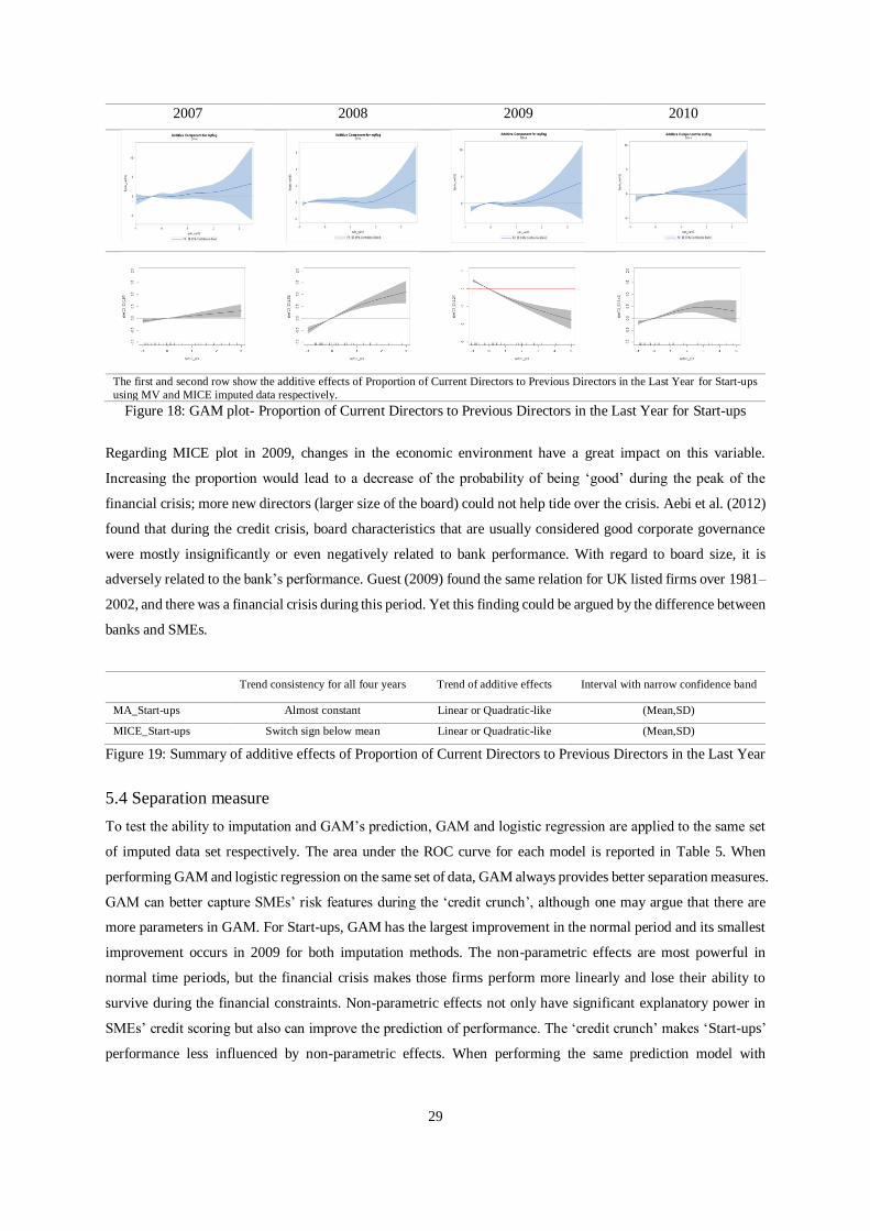
5.3.4 Proportion of Current Directors to Previous Directors in the Last Year

As seen from Figure 18, the additive effect shows a linear or quadratic -like trend, and a narrow confidence band

exists around the sample mean for both imputed methods. Except for the MICE imputed data in 2009, as the

proportion increases, the credit risk of Start-ups decreases, and their performance improves. Hence, if the board

of ‘Start-ups’ becomes constrained, the SME is more likely than others to fail. The confidence band becomes

much wider subsequently, which means prediction can be highly variable for firms with high liquidity in their

board.

29

2007 2008 2009 2010

The first and second row show the additive effects of Proportion of Current Directors to Previous Directors in the Last Year for Start-ups

using MV and MICE imputed data respectively. Figure 18: GAM plot- Proportion of Current Directors to Previous Directors in the Last Year for Start-ups

Regarding MICE plot in 2009, changes in the economic environment have a great impact on this variable.

Increasing the proportion would lead to a decrease of the probability of being ‘good’ during the peak of the

financial crisis; more new directors (larger size of the board) could not help tide over the crisis. Aebi et al. (2012)

found that during the credit crisis, board characteristics that are usually considered good corporate governance

were mostly insignificantly or even negatively related to bank performance. With regard to board size, it is

adversely related to the bank’s performance. Guest (2009) found the same relation for UK listed firms over 1981–

2002, and there was a financial crisis during this period. Yet this finding could be argued by the difference between

banks and SMEs.


MA_Start-ups Almost constant Linear or Quadratic-like (Mean,SD)

MICE_Start-ups Switch sign below mean Linear or Quadratic-like (Mean,SD)

Figure 19: Summary of additive effects of Proportion of Current Directors to Previous Directors in the Last Year

5.4 Separation measure

To test the ability to imputation and GAM’s prediction, GAM and logistic regression are applied to the same set

of imputed data set respectively. The area under the ROC curve for each model is reported in Table 5. When

performing GAM and logistic regression on the same set of data, GAM always provides better separation measures.

GAM can better capture SMEs’ risk features during the ‘credit crunch’, although one may argue that there are

more parameters in GAM. For Start-ups, GAM has the largest improvement in the normal period and its smallest

improvement occurs in 2009 for both imputation methods. The non-parametric effects are most powerful in

normal time periods, but the financial crisis makes those firms perform more linearly and lose their ability to

survive during the financial constraints. Non-parametric effects not only have significant explanatory power in

SMEs’ credit scoring but also can improve the prediction of performance. The ‘credit crunch’ makes ‘Start-ups’

performance less influenced by non-parametric effects. When performing the same prediction model with

30

different imputation techniques, MICE outperforms MV and the only exception is for Start-ups in 2009. The most

significant improvement is shown on the GAM model in 2007 for Start-ups.

Table 5 AUROC for logistic regression and general additive models

2007 2008 2009 2010

Start-ups

MA_LR 0.747 0.809 0.888 0.817

MA_GAM 0.760 0.820 0.896 0.827

MICE_LR 0.866 0.882 0.857 0.877

MICE_GAM 0.901 0.894 0.872 0.892

Non-Start-ups

MA_LR 0.777 0.795 0.859 0.797

MA_GAM 0.791 0.840 0.885 0.823

MICE_LR 0.808 0.881 0.886 0.857

MICE_GAM 0.844 0.912 0.918 0.870

6. SUMMARY AND DISCUSSION

Missing data has been a common phenomenon with SMEs data since often SMEs are not always willing or capable

to report their internal data and they do not have to release data to the market if they are not listed companies. In

this paper, we attempt to use two methods dealing with missing data: moving average and multiple imputation by

chained equations, and apply the imputed dataset on GAM by comparing to the logistic regression.

MA is a hot-deck single imputation technique related to WoE. It replaces the missing values by matching the

similar performance. This method is able to fill in the data points and easy to handle. However, it lacks theoretical

support and underestimates the standard errors and the variability if there is considerable missing data, such as

SMEs data. Besides, one drawback is that it is difficult to match performance if there are massive crossing points.

On the other hand, MICE is based on multiple imputation and to avoid imputations based on a single set of

regression parameters, an iterative algorithm uses Bayesian estimation to update the regression model parameters,

and it uses new estimates to generate each set of imputations. MICE is a flexible method. In the MICE procedures,

a series of regression models are performed thus each variable with missing data is modelled conditional on the

other variables in the data, which means each variable can be modelled according to its variable type. Our findings

have shown that MICE outperforms MV under the same prediction models.

By plotting, the variables’ trends are explained highlighting how SME’s performance varies. The variables’ trends

can help financial institutions identify their portfolio’s risk in a changing economy. For most variables, the

additive effect stays constant around the sample mean even through the ‘credit crunch’. Variables’ tail

performance is more sensitive to business cycles, the ‘credit crunch’ usually changes tails’ performance by

enlarging the confidence band or even changing the direction of influence. Their performance becomes less stable

due to the uncertainty of their supply chains through the ‘credit crunch’. For instance, firms which have longer

lateness of accounts, or which provided their last annual return some time ago, become opaque with regard to

their information from Companies House, and prediction bias is bigger for those firms. ‘Non-Start-ups' with

31

infrequent updates have a wider confidence band and those firms’ performance is less predictive. Considering that

all the information used in this research is ‘hard information’, this research suggests that ‘hard information’ is less

predictive for firms that update infrequently. In summary, the combination of MICE and GAM improves

prediction accuracy models even when missing categories are replaced with matching observed values and

demonstrates the marginal improvement in performance of independent variables.

REFERENCES

AALTO, J., PIRINEN, P., HEIKKINEN, J. & VENÄLÄINEN, A. (2013). Spatial interpolation of monthly climate data for Finland: comparing

the performance of kriging and generalized additive models. Theoretical and Applied Climatology, 112, 99-111.

AEBI, V., SABATO, G. & SCHMID, M. (2012). Risk management, corporate governance, and bank performance in the financial crisis.

Journal of Banking & Finance, 36, 3213-3226.

ALLISON, P. (2012). Why you probably need more imputations than you think. Statistical Horizons. Retrevied from http://statisticalhorizons.

com/more-imputations.

ALLISON, P. D. (2000). Multiple imputation for missing data: A cautionary tale. Sociological methods & research, 28, 301-309.

ALLISON, P. D. (2001). Missing data, Sage publications.

ANDREEVA, G., CALABRESE, R. & OSMETTI, S. A. (2016). A comparative analysis of the UK and Italian small businesses using

Generalised Extreme Value models. European Journal of Operational Research, 249, 506-516.

AUSTIN, P. C. (2007). A comparison of regression trees, logistic regression, generalized additive models, and multivariate adaptive regression

splines for predicting AMI mortality. Statistics in medicine, 26, 2937-2957.

AZUR, M. J., STUART, E. A., FRANGAKIS, C. & LEAF, P. J. (2011). Multiple imputation by chained equations: what is it and how does

it work? International journal of methods in psychiatric research, 20, 40-49.

BELLOTTI, T. & CROOK, J. (2009). Support vector machines for credit scoring and discovery of significant features. Expert Systems with

Applications, 36, 3302-3308.

BERG, D. (2007). Bankruptcy prediction by generalized additive models. Applied Stochastic Models in Business and Industry, 23, 129-143.

BODNER, T. E. (2008). What improves with increased missing data imputations? Structural Equation Modeling, 15, 651-675.

COX, D. R. (1958). The regression analysis of binary sequences. Journal of the Royal Statistical Society. Series B (Methodological), 215-242.

DOMINICI, F., MCDERMOTT, A., ZEGER, S. L. & SAMET, J. M. (2002). On the use of generalized additive models in time-series studies

of air pollution and health. American journal of epidemiology, 156, 193-203.

ENDERS, C. K. (2010). Applied missing data analysis, Guilford Press.

FRIEDMAN, J., HASTIE, T. & TIBSHIRANI, R. (2001). The elements of statistical learning, Springer series in statistics New York.

GRAHAM, J. W. (2009). Missing data analysis: Making it work in the real world. Annual review of psychology, 60, 549-576.

GRAHAM, J. W., OLCHOWSKI, A. E. & GILREATH, T. D. (2007). How many imputations are really needed? Some practical clarifications

of multiple imputation theory. Prevention science, 8, 206-213.

GREEN, P. J. & SILVERMAN, B. W. (1993). Nonparametric regression and generalized linear models: a roughness penalty approach, CRC

Press.

GUEST, P. M. (2009). The impact of board size on firm performance: evidence from the UK. The European Journal of Finance, 15, 385-404.

HASTIE, T. & TIBSHIRANI, R. (1986). Generalized Additive Models. Statistical Science, 1, 297-318.

HASTIE, T. & TIBSHIRANI, R. (1987). Generalized additive models: some applications. Journal of the American Statistical Association, 82,

371-386.

HASTIE, T. J. (2017). Generalized additive models. Statistical models in S. Routledge.

HE, Y., ZASLAVSKY, A. M., LANDRUM, M., HARRINGTON, D. & CATALANO, P. (2010). Multiple imputation in a large-scale complex

survey: a practical guide. Statistical methods in medical research, 19, 653-670.

HEITJAN, D. F. & LITTLE, R. J. (1991). Multiple imputation for the fatal accident reporting system. Applied Statistics, 13-29.

HORTON, N. J. & KLEINMAN, K. P. (2007). Much ado about nothing: A comparison of missing data methods and software to fit incomplete

data regression models. The American Statistician, 61, 79-90.

JAMES, G., WITTEN, D., HASTIE, T. & TIBSHIRANI, R. (2013). An introduction to statistical learning, Springer.

JELIČIĆ, H., PHELPS, E. & LERNER, R. M. (2009). Use of missing data methods in longitudinal studies: The persistence of bad practices

in developmental psychology. Developmental psychology, 45, 1195.

KEASEY, K. & WATSON, R. (1986). The prediction of small company failure: some behavioural evidence for the UK. Accounting and

Business Research, 17, 49-57.

LAZURE, A. (2017). Improving Credit Classification Using Machine Learning Techniques.

LEATHWICK, J., ELITH, J. & HASTIE, T. (2006). Comparative performance of generalized additive models and multivariate adaptive

regression splines for statistical modelling of species distributions. Ecological modelling, 199, 188-196.

LEE, K. J. & CARLIN, J. B. (2010). Multiple imputation for missing data: fully conditional specification versus multivariate normal

imputation. American journal of epidemiology, 171, 624-632.

LEE, T.-S., CHIU, C.-C., LU, C.-J. & CHEN, I.-F. (2002). Credit scoring using the hybrid neural discriminant technique. Expert Systems

with applications, 23, 245-254.

LITTLE, R. J. & RUBIN, D. B. (1987). Statistical analysis with missing data, John Wiley & Sons.

LITTLE, R. J. & RUBIN, D. B. (2014). Statistical analysis with missing data, John Wiley & Sons.

LONGFORD, N. T. (2006). Missing data and small-area estimation: Modern analytical equipment for the survey statistician, Springer Science

& Business Media.

MA, M. (2017). Through the crisis UK SMEs performance during the 'credit crunch'. PHD phd thesis, University of Edinburgh.

NEHREBECKA, N. (2018). Predicting the Default Risk of Companies. Comparison of Credit Scoring Models: Logit Vs Support Vector

Machines. Econometrics, 22, 54-73.

ONG, C.-S., HUANG, J.-J. & TZENG, G.-H. (2005). Building credit scoring models using genetic programming. Expert Systems with

Applications, 29, 41-47.

http://statisticalhorizons/

32

PAN, Q., WEI, R., SHIMIZU, I. & JAMOOM, E. (2014). Determining Sufficient Number of Imputations Using Variance of Imputation

Variances: Data from 2012 NAMCS Physician Workflow Mail Survey. Applied mathematics, 5, 3421.

PEUGH, J. L. & ENDERS, C. K. (2004). Missing data in educational research: A review of reporting practices and suggestions for

improvement. Review of educational research, 74, 525-556.

RAGHUNATHAN, T. E., LEPKOWSKI, J. M., VAN HOEWYK, J. & SOLENBERGER, P. (2001). A multivariate technique for multiply

imputing missing values using a sequence of regression models. Survey methodology, 27, 85-96.

RAMSAY, T. O., BURNETT, R. T. & KREWSKI, D. (2003). The effect of concurvity in generalized additive models linking mortality to

ambient particulate matter. Epidemiology, 14, 18-23.

RODWELL, L., LEE, K. J., ROMANIUK, H. & CARLIN, J. B. (2014). Comparison of methods for imputing limited-range variables: a

simulation study. BMC medical research methodology, 14, 57.

RUBIN, D. B. (1976). Inference and missing data. Biometrika, 63, 581-592.

RUBIN, D. B. (1987a). Multiple imputation for nonresponse in surveys, John Wiley & Sons.

RUBIN, D. B. (1987b). Multiple Imputation for Nonresponse in Surveys (Wiley Series in Probability and Statistics).

SCHAFER, J. L. (2003). Multiple imputation in multivariate problems when the imputation and analysis models differ. Statistica Neerlandica,

57, 19-35.

SCHAFER, J. L. & GRAHAM, J. W. (2002). Missing data: our view of the state of the art. Psychological methods, 7, 147.

SCHAFER, J. L. & OLSEN, M. K. (1998). Multiple imputation for multivariate missing-data problems: A data analyst's perspective.

Multivariate behavioral research, 33, 545-571.

SCHENKER, N. & TAYLOR, J. M. (1996). Partially parametric techniques for multiple imputation. Computational statistics & data analysis,

22, 425-446.

SOLANKI, H., BHATPURIA, D. & CHAUHAN, P. (2017). Applications of generalized additive model (GAM) to satellite-derived variables

and fishery data for prediction of fishery resources distributions in the Arabian Sea. Geocarto international, 32, 30 -43.

THOMAS, L. C. (2009). Consumer Credit Models: Pricing, Profit and Portfolios: Pricing, Profit and Portfolios, OUP Oxford.

TREVOR, H., ROBERT, T. & JH, F. (2009). The elements of statistical learning: data mining, inference, and prediction. New York, NY:

Springer.

VAN BUUREN, S. (2007). Multiple imputation of discrete and continuous data by fully conditional specification. Statistical methods in

medical research, 16, 219-242.

VINK, G., FRANK, L. E., PANNEKOEK, J. & BUUREN, S. (2014). Predictive mean matching imputation of semicontinuous variables.

Statistica Neerlandica, 68, 61-90.

VON HIPPEL, P. T. (2013). Should a normal imputation model be modified to impute skewed variables? Sociological Methods & Research,

42, 105-138.

WAHBA, G. (1990). Spline models for observational data, Siam.

WHITE, I. R., ROYSTON, P. & WOOD, A. M. (2011). Multiple imputation using chained equations: issues and guidance for practice.

Statistics in medicine, 30, 377-399.

WILKINSON, L. (1999). Statistical methods in psychology journals: Guidelines and explanations. American psychologist, 54, 594.

WOOD, A. M., WHITE, I. R. & THOMPSON, S. G. (2004). Are missing outcome data adequately handled? A review of published randomized

controlled trials in major medical journals. Clinical trials, 1, 368-376.

WOOD, S. & WOOD, M. S. (2015). Package ‘mgcv’. R package version, 1, 29.

WOOD, S. N. (2003). Thin plate regression splines. Journal of the Royal Statistical Society: Series B (Statistical Methodology), 65, 95-114.

WOOD, S. N. (2004). Stable and efficient multiple smoothing parameter estimation for generalized additive models. Journal of the American

Statistical Association, 99, 673-686.

WOOD, S. N. (2011). Fast stable restricted maximum likelihood and marginal likelihood estimation of semiparametric generalized linear

models. Journal of the Royal Statistical Society: Series B (Statistical Methodology), 73, 3-36.

WOOD, S. N. & AUGUSTIN, N. H. (2002). GAMs with integrated model selection using penalized regression splines and applications to

environmental modelling. Ecological modelling, 157, 157-177.

WOOD, S. N., PYA, N. & SÄFKEN, B. (2016). Smoothing parameter and model selection for general smooth models. Journal of the American

Statistical Association, 111, 1548-1563.

Date post:	25-Jun-2020
Category:	Documents
Upload:	others
View:	2 times
Download:	0 times

Addressing missing values in Credit Scoring · Missing data theory (Rubin, 1976) involves two sets...

Documents